algorithmic graph theory part i - review of basic notions in - profs
TRANSCRIPT

Algorithmic Graph TheoryPart I - Review of Basic Notions in Graph Theory,
Algorithms and Complexity
Martin [email protected]
University of Primorska, Koper, Slovenia
Dipartimento di InformaticaUniversita degli Studi di Verona, March 2013
1 / 75

What we’ll do
1 Overview.2 Basic Graph Theoretic Definitions.3 Algorithms - Basic Definitions.4 Graph Representations.5 Basics of Complexity.
1 / 75

Routing Problems
Source: http://lia.ei.uvigo.es/projects/vrp/index.html
2 / 75

Routing Problems
Source: http://lia.ei.uvigo.es/projects/vrp/index.html
2 / 75
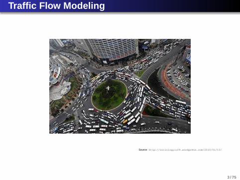
Traffic Flow Modeling
Source: http://sociologyiu09.wordpress.com/2010/01/13/
3 / 75

Social Networks
Source: http://kikolani.com/becoming-accessible-social-networking-social-media.html
5 / 75

Social Networks
Source: http://www.digitaltrainingacademy.com/socialmedia/2009/06/social_networking_map.php
5 / 75

Computer Networks
Source: http://www.uws.edu.au/organisational_development/od/how_to_register
5 / 75

World Wide Web
Source: http://website-in-a-weekend.net/wp-content/uploads/2009/11/network_nodes.jpg
6 / 75
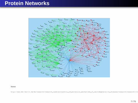
Protein Networks
Source:
http://www.mdc-berlin.de/de/research/research_teams/proteomics_and_molecular_mechanisms_of_neurodegenerative_diseases/research/research1/index.htm
7 / 75
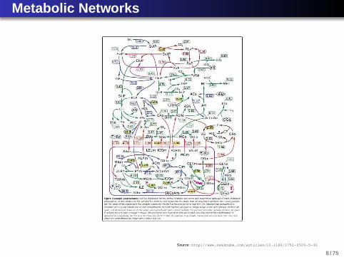
Metabolic Networks
Source: http://www.readcube.com/articles/10.1186/1752-0509-5-81
8 / 75
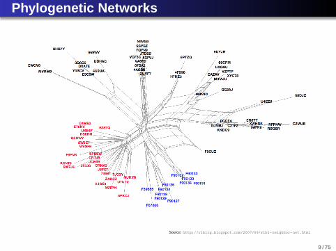
Phylogenetic Networks
Source: http://r1blog.blogspot.com/2007/09/r1b1-neighbor-net.html
9 / 75
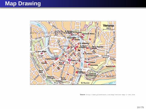
Map Drawing
Source: http://www.planetware.com/map/verona-map-i-ver.htm
10 / 75
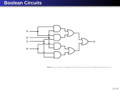
Boolean Circuits
Source: http://www.cci-compeng.com/Unit_2_Electronics/2405_Simplifying_Boolean.htm
11 / 75

What we’ll do – Week 1
1 Tue March 5: Review of basic notions in graph theory,algorithms and complexity
2 Wed March 6: Graph colorings
3 Thu March 7: Perfect graphs and their subclasses, part 1
4 Fri March 8: Perfect graphs and their subclasses, part 2
12 / 75

What we’ll do – Week 2
1 Tue March 19: Further examples of tractable problems,part 1
2 Wed March 20:Further examples of tractable problems, part 2Approximation algorithms for graph problems
3 Thu March 21: Lectio Magistralis lecture, “Graph classes:interrelations, structure, and algorithmic issues”
13 / 75

BASIC GRAPH THEORETIC DEFINITIONS.
13 / 75

Graphs
Graph: G = (V ,E) ordered pair, whereV = finite set of vertices ,E ⊆
(V2
)
(2-element subsets of V ) set of edges
Notation: V (G) = V , E(G) = E .
Example: V = 1,2,3,4, E = 1,2, 1,3, 2,3, 3,4
1 2
3
4
13 / 75
Graphs
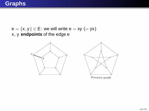
e = x , y ∈ E : we will write e = xy (= yx)x , y endpoints of the edge e
x
y
Petersen graph
14 / 75

Multigraphs
multigraphs :
parallel edges
loop
(E is a multisubset of(V
2
)
∪ V )
notation e = xy can be ambiguous for multigraphs; ifnecessary we use an incidence function: ψ(e) = xy
some authors use different terminology:graph = multigraphsimple graph = graph (without loops and parallel edges)
15 / 75

Digraphs
directed graphs (digraphs):D = (V ,A)V : vertices, A: directed edgesA ⊆ V × V
A digraph is simple if it has no loops and no directed paralleledges.
16 / 75
Neighborhoods and Degrees
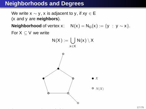
We write x ∼ y , x is adjacent to y , if xy ∈ E(x and y are neighbors ).
Neighborhood of vertex x : N(x) = NG(x) := y : y ∼ x.
For X ⊆ V we write
N(X ) :=⋃
x∈X
N(x) \ X
X
N(X)
(We remove X from N(X )!)17 / 75

Handshaking Lemma
The degree of vertex x : d(x) = dG(x) := |NG(x)|.A vertex v is isolated if d(v) = 0.
Handshaking Lemma: For every graph G = (V ,E),∑
x∈V
d(x) = 2 · |E | .
Proof:∑
x d(x) =∑
x∑
y∼x 1 = 2 · |E |.
Corollary:The number of vertices of odd degree in a graph is even.
18 / 75

Degrees in Digraphs
If D = (V ,A) is a digraph, we define:
N+(x) := y ∈ V : xy ∈ A successors of vertex x
N−(x) := y ∈ V : yx ∈ A predecessors of vertex x
out-degree of vertex x : d+(x) := |N+(x)|
in-degree of vertex x : d−(x) := |N−(x)|
19 / 75
Isomorphisms
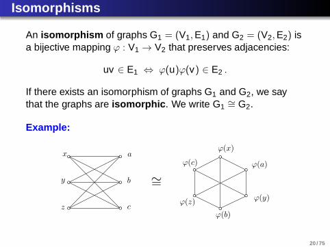
An isomorphism of graphs G1 = (V1,E1) and G2 = (V2,E2) isa bijective mapping ϕ : V1 → V2 that preserves adjacencies:
uv ∈ E1 ⇔ ϕ(u)ϕ(v) ∈ E2 .
If there exists an isomorphism of graphs G1 and G2, we saythat the graphs are isomorphic . We write G1
∼= G2.
Example:
x
y
z
a
b
c
ϕ(x)
ϕ(y)ϕ(z)
ϕ(a)
ϕ(b)
ϕ(c)
∼=
20 / 75
Isomorphisms
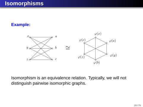
Example:
x
y
z
a
b
c
ϕ(x)
ϕ(y)ϕ(z)
ϕ(a)
ϕ(b)
ϕ(c)
∼=
Isomorphism is an equivalence relation. Typically, we will notdistinguish pairwise isomorphic graphs.
20 / 75
Subgraphs
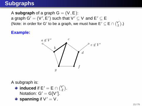
A subgraph of a graph G = (V ,E):a graph G′ = (V ′,E ′) such that V ′ ⊆ V and E ′ ⊆ E(Note: in order for G′ to be a graph, we must have E ′ ⊆ E ∩
(V ′
2
)
.)
Example:
a 6∈ V ′
b
c
d
e 6∈ V ′
fg
A subgraph is:induced if E ′ = E ∩
(V ′
2
)
.Notation: G′ = G[V ′].spanning if V ′ = V .
21 / 75
Walks, Trails and Paths
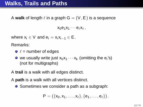
A walk of length ℓ in a graph G = (V ,E) is a sequence
x0e1x1 · · · eℓxℓ ,
where xi ∈ V and ei = xi xi−1 ∈ E .
Remarks:
ℓ = number of edges
we usually write just x0x1 · · · xk (omitting the ei ’s)(not for multigraphs)
A trail is a walk with all edges distinct.
A path is a walk with all vertices distinct.
Sometimes we consider a path as a subgraph:
P = (x0, x1, . . . , xℓ, e1, . . . ,eℓ) .
22 / 75
Walks, Trails and Paths
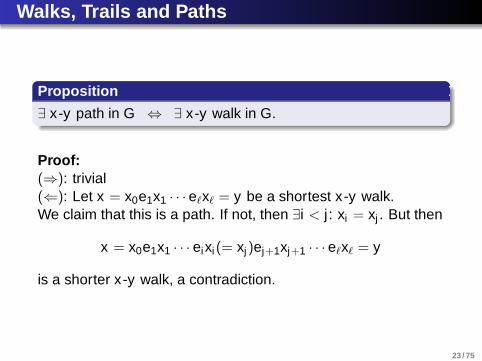
Proposition
∃ x-y path in G ⇔ ∃ x-y walk in G.
Proof:(⇒): trivial(⇐): Let x = x0e1x1 · · · eℓxℓ = y be a shortest x-y walk.We claim that this is a path. If not, then ∃i < j : xi = xj . But then
x = x0e1x1 · · · eixi(= xj)ej+1xj+1 · · · eℓxℓ = y
is a shorter x-y walk, a contradiction.
23 / 75

Cycles
A walk is closed if xℓ = x0.
A cycle : a closed trail such that x0x1 · · · xℓ−1 is a path.
ℓ ≥ 3, except for multigraphs, where we can also haveℓ = 1 (loop) and ℓ = 2 (a pair of parallel edges).
When defining paths and cycles in digraphs we take intoaccount directions of edges.
24 / 75
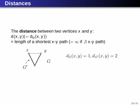
Distances
The distance between two vertices x and y :d(x , y)(= dG(x , y))= length of a shortest x-y path (= ∞ if 6 ∃ x-y path)
x y
G
G′
dG(x, y) = 1, dG′(x, y) = 2
25 / 75

Components
A graph is connected if for every two vertices u, v ∈ V (G)there exists a path between them.
[x is a path of length 0]
Components of a graph G: maximal connected subgraphs
26 / 75
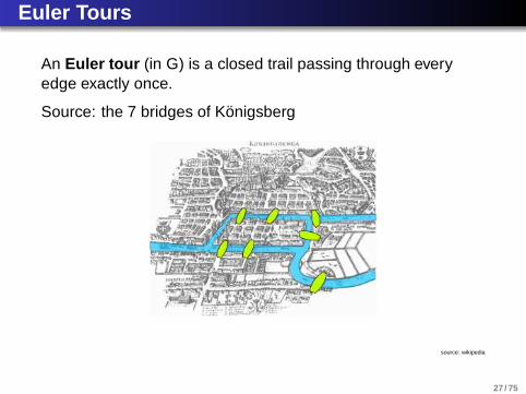
Euler Tours
An Euler tour (in G) is a closed trail passing through everyedge exactly once.
Source: the 7 bridges of Konigsberg
source: wikipedia
27 / 75
Euler Tours
Theorem (Euler, 1736)
A multigraph G without isolated vertices has an Euler tour ⇔G is connected and all vertices are of even degree.
Hence, the obvious necessary condition is also sufficient.
28 / 75
Hamiltonian Cycles
Hamiltonian cycle : a cycle going through every vertex exactlyonce.
Can we give a simple necessary and sufficient condition for theexistence of a Hamiltonian cycle in a graph?
Most likely not, since the decision problem whether a givengraph is Hamiltonian is NP-complete.
29 / 75

Operations on Graphs
The complement of a graph G = (V ,E) is the graphG = (V ,
(V2
)
\ E).(This is the graph with the same vertex set as G, in which twovertices are adjacent if and only if they are not adjacent in G.)
Example:
G G
v1
v2
v3
v4
v5 v1
v2
v3
v4
v5
30 / 75
Operations on Graphs
v ∈ V : G − v = the subgraph of G induced by the vertex setV \ v.
Similarly, we have G − U = G[V \ U] for U ⊆ V .
G − e = (V ,E \ e) for e ∈ E (spanning subgraph)
Similarly, G − F = (V ,E \ F ) for F ⊆ E .
31 / 75

Operations on Graphs
union of graphs:G ∪ H: graph (V (G) ∪ V (H),E(G) ∪ E(H))
intersection of graphs:G ∩ H: graph (V (G) ∩ V (H),E(G) ∩ E(H))
G + H: disjoint union of graphs G and H(Formally:V (G + H) = (V (G)× 1) ∪ (V (H)× 2),
E(G + H) = (u, 1)(v ,1) : uv ∈ E(G) ∪ (u, 2)(v , 2) : uv ∈ E(H))
G ∗ H join of graphs G and H:disjoint union of graphs G and H together with all possibleedges between V (G)× 1 and V (H)× 2
32 / 75

Complete and Complete Bipartite Graphs
A complete graph :KV := (V ,
(V2
)
), we usually write just Kn where n = |V |nG:= disjoint union of n copies of a graph G
K2 2K2
Complete bipartite graph : Km,n:graph G = (V ,E) such thatV = A ∪ B, A ∩ B = ∅, |A| = m, |B| = n andE = ab : a ∈ A,b ∈ B.
33 / 75
Paths and Cycles
Path Pn: graph G = (V ,E) withV = v1, . . . , vn andE = v1v2, . . . , vn−1vn.
Cycle Cn:graph G = (V ,E) withV = v1, . . . , vn andE = v1v2, . . . , vn−1vn, vnv1.
34 / 75
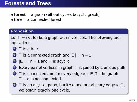
Forests and Trees
a forest = a graph without cycles (acyclic graph)a tree = a connected forest
Proposition
Let T = (V ,E) be a graph with n vertices. The following areequivalent:
1 T is a tree.2 T is a connected graph and |E | = n − 1.3 |E | = n − 1 and T is acyclic.4 Every pair of vertices in graph T is joined by a unique path.5 T is connected and for every edge e ∈ E(T ) the graph
T − e is not connected.6 T is an acyclic graph, but if we add an arbitrary edge to T ,
we obtain exactly one cycle.
35 / 75
ALGORITHMS - BASIC DEFINITIONS.
35 / 75
Algorithms
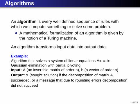
An algorithm is every well defined sequence of rules withwhich we compute something or solve some problem.
A mathematical formalization of an algorithm is given bythe notion of a Turing machine.
An algorithm transforms input data into output data.
Example:Algorithm that solves a system of linear equations Ax = b:Gaussian elimination with partial pivotingInput: A (an invertible matrix of order n), b (a vector of order n)Output: x (sought solution) if the decomposition of matrix Asucceeded, or a message that due to rounding errors decompositiondid not succeed
36 / 75
Algorithms
We require from an algorithm that it stops after a finite numberof calculation steps.
When developing an algorithm for a given problem, we shouldalso provide:
an analysis of the time complexity of the algorithm;
a proof of correctness .
The algorithms can be described either in the natural languageor in pseudocode.
37 / 75

Algorithms
Example:An algorithm that computes the product C of two squarematrices A and B of order n:
MATRIX MULTIPLICATION
Input: Real matrices A and B of size n × n.Output: Matrix C = A · B.for i = 1, . . . , n do
for j = 1, . . . , n doC[i, j] := A[i, 1] · B[1, j];for k = 2, . . . , n do
C[i, j] := C[i, j] + A[i, k ] · B[k , j];end for
end forend forreturn C;
The algorithm makes n3 multiplications and n2(n − 1) additions.Proof of correctness is obvious.
38 / 75

Instances and Their Sizes
We are given an (optimization, decision, ...) problem P.Examples:
“Compute the product of two given matrices of order n.”
“Find the smallest number among n given rationalnumbers.”
“Determine whether the given graph G has a Hamiltoniancycle.”
instance: concrete input data for problem P
size of the instance: the number of bits needed to store theinstance in the computer.
We need to choose an appropriate way of representing theinstance.
39 / 75

Representing the Instances
Examples:
We usually store a positive integer n with ⌊log2 n⌋+ 1 bits(sometimes also with n bits as 11 · · · 1 (n ones)).
We can store a matrix of n2 positive integers with at mostn2 log2 M bits where M is the biggest number in the matrix.
Or: with a set of triples (i , j ,aij) : aij 6= 0.This representation is particularly suitable for matrices withmany zero elements.
We can represent a graph in several ways (more about thislater).
40 / 75
Time Complexity of Algorithms
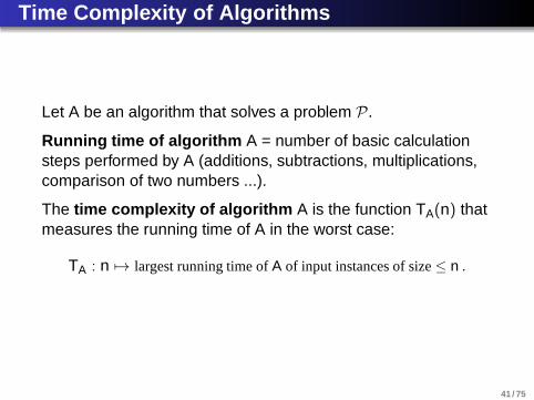
Let A be an algorithm that solves a problem P.
Running time of algorithm A = number of basic calculationsteps performed by A (additions, subtractions, multiplications,comparison of two numbers ...).
The time complexity of algorithm A is the function TA(n) thatmeasures the running time of A in the worst case:
TA : n 7→ largest running time of A of input instances of size ≤ n .
41 / 75

Time Complexity of Algorithms
Remarks:
Besides time complexity, space complexity of analgorithm might also be important (how much computermemory the algorithm needs).
If we have a probability distribution on the input instances,we can also estimate the expected time complexity ofthe algorithm.
42 / 75

Big O Notation
A function f : N → N is of order (at most) O(g), if there existsa constant C > 0 such that f (n) ≤ C · g(n) for all n ∈ N.
Notation: f = O(g)
If f = O(g), we also write g ∈ Ω(f ) and say that g is of order(at least) Ω(f ).
Two functions f and g are of the same order if f = O(g) andf = Ω(g). Notation: f = Θ(g).
43 / 75
Big O Notation
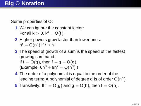
Some properties of O:
1 We can ignore the constant factor:For all k > 0, kf = O(f ).
2 Higher powers grow faster than lower ones:nr = O(ns) if r ≤ s.
3 The speed of growth of a sum is the speed of the fastestgrowing summand:If f = O(g), then f + g = O(g).(Example: 6n3 + 9n2 = O(n3).)
4 The order of a polynomial is equal to the order of theleading term: A polynomial of degree d is of order O(nd ).
5 Transitivity: If f = O(g) and g = O(h), then f = O(h).
44 / 75

Big O Notation
6 Exponential functions grow faster than power functions:For all k ≥ 0, b > 1, it holds nk = O(bn).(Example: n4 = O(2n), n4 = O(en), n4 = O(1.0001n).)
7 Logarithms grow slower than power functions:For all k > 0, b > 1, it holds logb n = O(nk ).(Example: log2 n = O(n1/2).)
8 Logarithms are of the same order:For all b,d > 1, it holds logb n = O(logd n).
9 If f = O(g) and h = O(r), then fh = O(gr).(Example: if f = O(n2) and g = O(log n), thenfg = O(n2 log n).)
45 / 75
Typical Time Complexities
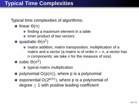
Typical time complexities of algorithms:linear Θ(n)
finding a maximum element in a tableinner product of two vectors
quadratic Θ(n2)
matrix addition, matrix transposition, multiplication of amatrix and a vector (a matrix is of order n × n, a vector hasn components; we take n for the measure of size)
cubic Θ(n3)
typical matrix multiplication
polynomial O(p(n)), where p is a polynomial
exponential O(2p(n)), where p is a polynomial ofdegree ≥ 1 with positive leading coefficient
46 / 75
Polynomial Algorithms
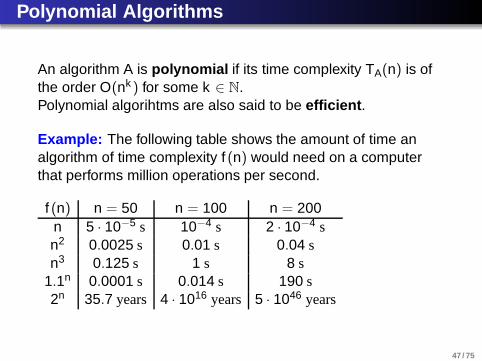
An algorithm A is polynomial if its time complexity TA(n) is ofthe order O(nk ) for some k ∈ N.Polynomial algorihtms are also said to be efficient .
Example: The following table shows the amount of time analgorithm of time complexity f (n) would need on a computerthat performs million operations per second.
f (n) n = 50 n = 100 n = 200n 5 · 10−5 s 10−4 s 2 · 10−4 sn2 0.0025 s 0.01 s 0.04 sn3 0.125 s 1 s 8 s
1.1n 0.0001 s 0.014 s 190 s2n 35.7 years 4 · 1016 years 5 · 1046 years
47 / 75

Polynomial Algorithms
On a 1000 times faster computer:
f (n) n = 50 n = 100 n = 200n 5 · 10−8 s 10−7 s 2 · 10−7 sn2 2.5 · 10−6 s 10−5 s 4 · 10−5 sn3 1.25 · 10−4 s 10−3 s 8 · 10−3 s
1.1n 1.1 · 10−7 s 1.4 · 10−5 s 0.19 s2n 13 days 4 · 1013 years 5 · 1043 years
48 / 75

GRAPH REPRESENTATIONS.
48 / 75
Graph Representations
How to represent a graph in a computer?This depends on what graphs we will work with and whatoperations we want to preform on them.
Let G = (V ,E) whereV = v1, . . . , vn,E = e1, . . . ,em.
49 / 75

Adjacency Matrix A(G)
Adjacency matrix of a graph G:
A(G) =
a11 a12 . . . a1n
a21 a22 . . . a2n...
.... . .
...an1 an2 . . . ann
, aij =
1, if vi ∼ vj ;0, otherwise.
Order of magnitude of this representation: O(n2)
50 / 75
Adjacency Matrix A(G)
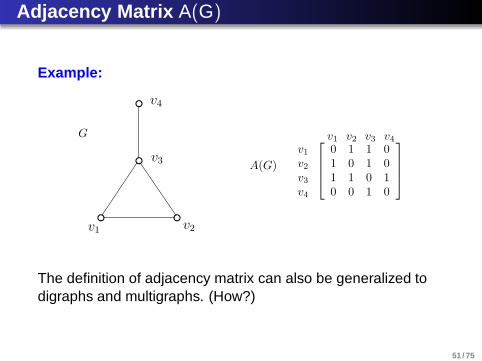
Example:
v1v2
v3
v4
v1
v2
v3
v4
0 1 1 01 0 1 01 1 0 10 0 1 0
v1 v2 v3 v4G
A(G)
The definition of adjacency matrix can also be generalized todigraphs and multigraphs. (How?)
51 / 75
Adjacency List Representation
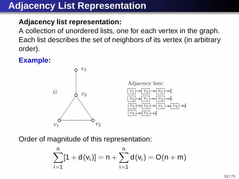
Adjacency list representation:A collection of unordered lists, one for each vertex in the graph.Each list describes the set of neighbors of its vertex (in arbitraryorder).
Example:
v1v2
v3
v4
G
Adjacency lists:
v1
v2
v3
v4
v2
v2
v1
v1
v3
v3
v3
v4
Order of magnitude of this representation:n
∑
i=1
[1 + d(vi)] = n +n
∑
i=1
d(vi) = O(n + m)
52 / 75
Adjacency List Representation
This representation is particularly useful for sparse graphs(graphs with O(n) edges).
Many useful graphs are “sparse”:
In a country there are several 1000 cities, but only a smallnumber of roads goes out of each city.
In Italy there are about 60 million people, but each personhas only several 10 or several 100 acquaintances.
The adjacency list representation can also be generalized todigraphs and multigraphs. (How?)
53 / 75

Comparison of Representations
With adjacency matrix representation each of the followingoperations takes constant time O(1):
1 check if vi ∼ vj ,2 remove an edge,3 add an edge.
With adjacency list representation we need the followingtime for the three operations:
1 O(d(vi)), since we need to traverse the list of neighbors ofvi (or vj ),
2 O(maxd(vi), d(vj)), since we need to traverse both listsof neighbors (of vi and of vj ),
3 O(1), since we need to add vertex vi on the list ofneighbors of vj and vice versa
54 / 75

Comparison of Representations
The space complexity of the adjacency matrix representation isΘ(n2), independently of the number of edges.The space complexity of the adjacency list representation isO(n + m), which is O(n) for sparse graphs.
We say that a graph problem is solvable in linear time if it canbe solved by an algorithm of time complexity O(n + m) (wheren = |V |,m = |E |).
We assume adjacency list representation.
55 / 75

BASICS OF COMPLEXITY.
55 / 75

Decision Problems, Classes P, NP, and co- NP
Decision problem : a problem in which the set of instancesdivides into two sets depending on whether the answer is YESor NO.
We define three classes of decision problems:
P is the set of decision problems that can be solved by apolynomial algorithmIntuitively: P is the set of problems that can be solvedefficiently.
56 / 75

Decision Problems, Classes P, NP, and co- NP
Decision problem : a problem in which the set of instancesdivides into two sets depending on whether the answer is YESor NO.
We define three classes of decision problems:
NP is the set of decision problems with the followingproperty:If the answer is YES then there exists a certificate thatenables us to verify this fact in polynomial time.
56 / 75

Decision Problems, Classes P, NP, and co- NP
Decision problem : a problem in which the set of instancesdivides into two sets depending on whether the answer is YESor NO.
We define three classes of decision problems:
NP is the set of decision problems with the followingproperty:If the answer is YES then there exists a certificate thatenables us to verify this fact in polynomial time.Intuitively: NP is the set of problems for which we canquickly verify a positive answer if we are given a solution.
56 / 75
Decision Problems, Classes P, NP, and co- NP
Decision problem : a problem in which the set of instancesdivides into two sets depending on whether the answer is YESor NO.
We define three classes of decision problems:
NP is the set of decision problems with the followingproperty:If the answer is YES then there exists a certificate thatenables us to verify this fact in polynomial time.Intuitively: NP is the set of problems for which we canquickly verify a positive answer if we are given a solution.(Formally: NP is the set of languages recognizable by some Turing
machine in polynomial time.)
56 / 75

Decision Problems, Classes P, NP, and co- NP
Decision problem : a problem in which the set of instancesdivides into two sets depending on whether the answer is YESor NO.
We define three classes of decision problems:
co-NP is the set of decision problems with the followingproperty:If the answer is NO then there exists a certificate thatenables us to verify this fact in polynomial time.
56 / 75
Some Polynomial Graph Problems
The following problems are all in P:
TOPOLOGICAL SORT: find an ordering of the vertices of agiven digraph such that the first endpoint of each edge willprecede the last endpoint in the order
BREADTH-FIRST SEARCH (BFS): systematically checkeverything reachable from a given starting vertex
DEPTH-FIRST SEARCH (DFS): like BFS, but in a differentorder
SHORTEST PATHS: every edge has a length, find a shortestpath between two vertices
57 / 75
Some Polynomial Graph Problems (cont’d)
The following problems are all in P:
MINIMUM SPANNING TREE: every edge has a length, find aset of edges with minimum total length such that everyvertex is covered by an edge
MAXIMUM FLOW: every (directed) edge has a capacity, findthe maximum amount of flow from a source to a sink sothat the conservation of flow is preserved
MAXIMUM MATCHING: find a largest set of pairwise disjointedges in a graph
57 / 75
Example of a Problem in NP
Example:
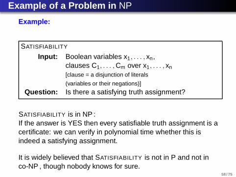
SATISFIABILITY
Input: Boolean variables x1, . . . , xn,clauses C1, . . . ,Cm over x1, . . . , xn
[clause = a disjunction of literals
(variables or their negations)]
Question: Is there a satisfying truth assignment?
SATISFIABILITY is in NP :If the answer is YES then every satisfiable truth assignment is acertificate: we can verify in polynomial time whether this isindeed a satisfying assignment.
It is widely believed that SATISFIABILITY is not in P and not inco-NP , though nobody knows for sure.
58 / 75
Decision Problems, Classes P, NP, and co- NP
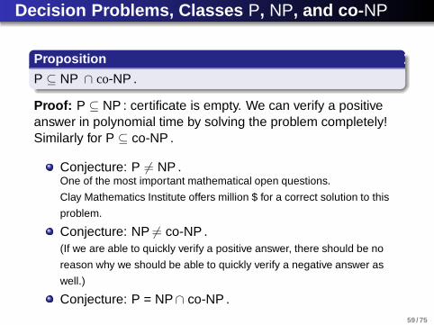
Proposition
P ⊆ NP ∩ co-NP .
Proof: P ⊆ NP : certificate is empty. We can verify a positiveanswer in polynomial time by solving the problem completely!Similarly for P ⊆ co-NP .
Conjecture: P 6= NP .One of the most important mathematical open questions.
Clay Mathematics Institute offers million $ for a correct solution to this
problem.
Conjecture: NP 6= co-NP .(If we are able to quickly verify a positive answer, there should be no
reason why we should be able to quickly verify a negative answer as
well.)
Conjecture: P = NP∩ co-NP .
59 / 75

Decision Problems, Classes P, NP, and co- NP
Jack Edmonds believes P = NP∩ co-NP :
Source: http://pretty.structures.free.fr/photos/photos6.html
60 / 75
NP-hard Problems
A problem Π is NP-hard ifthe existence of a polynomial algorithm for Π would implythe existence of a polynomial algorithm for every problem inNP .
In other words:
Π is NP-hard ⇔If Π is solvable in polynomial time then P = NP .
Intuitively: if we could solve efficiently just one NP-hard problem Π, thenwe would be able to solve efficiently every problem whose solution wecan verify quickly, by means of an algorithm for problem Π.
NP-hard problems are at least as hard as an arbitrary problem in NP.
61 / 75

NP-complete Problems
A problem is NP-complete if it is NP-hard and it belongs to NP.
These are the hardest problems in NP.
If there exists a polynomial time algorithm for just oneNP-complete problem, then all NP-complete problems arepolynomially solvable.
Thousands of NP-complete problems are known.A polynomial algorithm for either of them is very unlikely.
62 / 75
NP-complete Problems
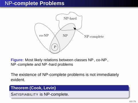
co-NP NP
P
NP-hard
NP-complete
Figure: Most likely relations between classes NP , co-NP ,NP -complete and NP -hard problems
The existence of NP-complete problems is not immediatelyevident.
Theorem (Cook, Levin)
SATISFIABILITY is NP-complete.
63 / 75
Polynomial Reductions
Π1, Π2 decision problems
DefinitionProblem Π1 is polynomially reducible to Π2, if for everyinstance I for Π1 we can construct in polynomial time aninstance J = J(I) for problem Π2 such that the answer to Π1
given I is the same as the answer to Π2 given J.
Notation: Π1 ∝ Π2.
64 / 75
Polynomial Reductions
To show that a problem Π ∈ NP is NP -complete,we reduce a known NP -complete problem to Π.
Proposition
Suppose that for a problem Π ∈ NP there exists anNP -complete problem Π1 such that Π1 ∝ Π. Then Π isNP-complete.
65 / 75
Examples of NP-complete Problems
INDEPENDENT SET
Input: Graph G = (V ,E), k ∈ N
Question: Does G contain an independent set of size k?
independent set: a subset I ⊆ V such that u, v ∈ I ⇒ uv 6∈ E
Proposition
The INDEPENDENT SET problem is NP -complete.
Proof:1. INDEPENDENT SET ∈ NP : we can verify in polynomial timewhether I is an independent set of size k .
66 / 75

Examples of NP-complete Problems
2. Reduction from SATISFIABILITY.Example:The set of clauses
x1 ∨ x2 , x2 ∨ x3 ∨ x4 , x1 ∨ x3 ∨ x4 , x1 ∨ x2 ∨ x3 ∨ x4
over the variables x1, x2, x3, x4 gets mapped to (G,4), where 4is the number of clauses and G is the following graph:
x1
x1
x2
x2
x3
x4
x1
x3
x4
x3
x2
x4
x1
x1
x2
x4
67 / 75

Examples of NP-complete Problems (cont’d)
CLIQUE
Input: Graph G = (V ,E), k ∈ N
Question: Does G contain a clique of size k?
clique: a subset C ⊆ V such thatu, v ∈ C ∧ u 6= v ⇒ uv ∈ E
Proposition
The CLIQUE problem is NP -complete.
Proof:1. CLIQUE ∈ NP : we can verify in polynomial time whether C isa clique of size k .2. INDEPENDENT SET ∝ CLIQUE
I = (G, k) instance for INDEPENDENT SET 7→J(I) = (G, k) instance for CLIQUE
68 / 75
Examples of NP-complete Problems (cont’d)
VERTEX COVER
Input: Graph G = (V ,E), k ∈ N
Question: Does G contain a vertex cover of size k?
vertex cover: a subset C ⊆ V such that for all e ∈ E , e ∩C 6= ∅
Proposition
The VERTEX COVER problem is NP -complete.
Proof:1. VERTEX COVER ∈ NP : we can verify in polynomial timewhether C is a vertex cover of size k .2. INDEPENDENT SET ∝ VERTEX COVER
I = (G = (V ,E), k) instance for INDEPENDENT SET 7→J(I) = (G, |V | − k) instance for VERTEX COVER
69 / 75

Examples of NP-complete Problems (cont’d)
DOMINATING SET
Input: Graph G = (V ,E), k ∈ N
Question: Does G contain a dominating set of size k?
dominating set: a set D ⊆ V such that every vertex is either inD or has a neighbor in D
Proposition
The DOMINATING SET problem is NP -complete.
Proof:1. DOMINATING SET ∈ NP :we can verify in polynomial time whether D is a dominating setof size k .
70 / 75
Examples of NP-complete Problems (cont’d)
2. VERTEX COVER ∝ DOMINATING SET
I = (G = (V ,E), k) instance for VERTEX COVER 7→J(I) = (G′ = (V ′,E ′), k) instance for DOMINATING SET where:
V ′ = V ∪ E ,
V is a clique in G′,
E is an independent set in G′,
ve ∈ E(G′) ⇔ v ∈ V ,e ∈ E , v is an endpoint of e.
71 / 75
Some Further NP-complete Problems
The following problems are NP-complete:
3-SATISFIABILITY: just like SATISFIABILITY, except thatevery clause consists of exactly 3 literals
(2-SATISFIABILITY ∈ P.)
3-COLORABILITY: can the vertex set of a given graph bepartitioned into 3 (possibly empty) independent sets?
(2-COLORABILITY ∈ P.)
HAMILTIONIAN CYCLE: does a given graph have aHamiltonian cycle?
72 / 75
Some Further NP-complete Problems (cont’d)
The following problems are NP-complete:
TRAVELING SALESMAN: does a given edge-weighted graphhave a Hamiltonian cycle of total length ≤ L
METRIC TRAVELING SALESMAN: like TRAVELING
SALESMAN, except that the lengths satisfy triangleinequality
MAX CUT: does a given graph admit a partition of its vertexset into two sets such that there are at least k edgesbetween them?
72 / 75
How to Deal With NP -complete Problems?
There are several approaches on how to deal with theintractability of NP -complete problems:
polynomial algorithms for particular input instances
approximation algorithms
heuristics, local optimization
“efficient” exponential algorithms (e.g., 1.5n instead of 2n)
randomized algorithms
parameterized complexity(fixed-parameter tractable (FPT) algorithms)
73 / 75

What we’ll do – Week 1
1 Tue March 5: Review of basic notions in graph theory,algorithms and complexity X
2 Wed March 6: Graph colorings
3 Thu March 7: Perfect graphs and their subclasses, part 1
4 Fri March 8: Perfect graphs and their subclasses, part 2
74 / 75
What we’ll do – Week 2
1 Tue March 19: Further examples of tractable problems,part 1
2 Wed March 20:Further examples of tractable problems, part 2Approximation algorithms for graph problems
3 Thu March 21: Lectio Magistralis lecture, “Graph classes:interrelations, structure, and algorithmic issues”
75 / 75