alexandre de carvalho, alberto sanyuan suen e felippe gallo … · 2016-05-17 · alexandre de...

Market Efficiency in Brazil: some evidence from high-frequency data

Alexandre de Carvalho, Alberto Sanyuan Suen e Felippe Gallo

May, 2016

431

ISSN 1518-3548 CGC 00.038.166/0001-05

Working Paper Series Brasília n. 431 May 2016 p. 1-31

Working Paper Series Edited by Research Department (Depep) – E-mail: [email protected] Editor: Francisco Marcos Rodrigues Figueiredo – E-mail: [email protected] Editorial Assistant: Jane Sofia Moita – E-mail: [email protected] Head of Research Department: Eduardo José Araújo Lima – E-mail: [email protected] The Banco Central do Brasil Working Papers are all evaluated in double blind referee process. Reproduction is permitted only if source is stated as follows: Working Paper n. 431. Authorized by Altamir Lopes, Deputy Governor for Economic Policy. General Control of Publications Banco Central do Brasil

Comun/Dipiv/Coivi

SBS – Quadra 3 – Bloco B – Edifício-Sede – 14º andar

Caixa Postal 8.670

70074-900 Brasília – DF – Brazil

Phones: +55 (61) 3414-3710 and 3414-3565

Fax: +55 (61) 3414-1898

E-mail: [email protected]

The views expressed in this work are those of the authors and do not necessarily reflect those of the Banco Central or its members. Although these Working Papers often represent preliminary work, citation of source is required when used or reproduced. As opiniões expressas neste trabalho são exclusivamente do(s) autor(es) e não refletem, necessariamente, a visão do Banco Central do Brasil. Ainda que este artigo represente trabalho preliminar, é requerida a citação da fonte, mesmo quando reproduzido parcialmente. Citizen Service Division Banco Central do Brasil

Deati/Diate

SBS – Quadra 3 – Bloco B – Edifício-Sede – 2º subsolo

70074-900 Brasília – DF – Brazil

Toll Free: 0800 9792345

Fax: +55 (61) 3414-2553

Internet: <http//www.bcb.gov.br/?CONTACTUS>

Market Efficiency in Brazil: some evidence from high-frequency data*

Alexandre de Carvalho**

Alberto Sanyuan Suen***

Felippe Gallo

Abstract

The Working Papers should not be reported as representing the views of the Banco Central do Brasil. The views expressed in the papers are those of the authors and do not necessarily reflect those of the Banco Central do Brasil.

In this paper we used intraday data to assess market efficiency in Brazil. We used a database of prices and the number of shares traded of liquid stocks listed in Brazil’s stock exchange, BM&FBOVESPA, and disclosures of material facts legally imposed by the Comissão de Valores Mobiliários (CVM), the Brazilian authority for the regulation of security markets. Our findings indicate material facts reported by firms indeed reveal unexpected information to investors. The speed of price response to new information and the observed magnitudes of cumulative returns indicate market participants can benefit from profit opportunities in the minutes close to the release of material facts. Our findings suggest stock prices take up to fifty minutes to incorporate the new information. Keywords: market efficiency; event studies; intraday data. JEL Classification: G14

* We thank Fernando Postali, Leonardo Nogueira Ferreira, Vinicius Brandi and an anonymous referee for helpful comments. All remaining errors rest with the authors. ** Central Bank of Brazil, e-mail: [email protected] *** Department of Economics, Universidade Federal do ABC (UFABC), e-mail:[email protected]. Department of Information Engineering, Universidade Federal do ABC (UFABC), e-mail: [email protected]

3

1. Introduction

The hypothesis of efficient markets has been investigated at length since the late

sixties, mainly after studies by Fama et al. (1969) and Fama (1970). In this paper we use

intraday stock returns and a set of compulsory releases of material facts by publicly

traded companies to assess market efficiency in Brazil. Specifically, we examine the

semi-strong form of market efficiency by means of an event study, seeking primarily to

evaluate how fast stock prices fully reflect all information publicly available.

Our empirical analysis builds on a high-frequency database, including minute-

to-minute data on transaction prices and the number of shares traded of liquid stocks

listed in Brazil’s stock exchange, the Bolsa de Valores, Mercadorias e Futuros de Sao

Paulo—BM&FBOVESPA. All intraday price and volume data were collected through

computational routines from November 2012 to February 2014.

We pooled high-frequency data on stock prices and traded volumes with a set of

public releases of material facts, provided by the regulatory authority of security

markets in Brazil, the Comissão de Valores Mobiliários (CVM). Publicly traded

companies are required by the CVM to fully disclose material facts to reduce

informational asymmetries and insider trading. In practice, as soon as facts are

recognized as material by publicly traded firms, files describing them must be

electronically sent to the CVM, prior to disclosures in other communication channels,

by means of an electronic system developed for this finality. After sending, files are

immediately displayed on the websites of the CVM and BM&FBOVESPA along with

the subject, day, hour and minute of every disclosure.

In order to perform our event study, we collected intraday transaction prices,

traded volumes and the time of compulsory releases by publicly traded firms.

Information on material facts was collected directly from the CVM’s website. Our

intraday data refer to the last transaction price and accumulated traded volume in each

single minute. The combination of these two sets of financial information enabled us to

evaluate how fast, in minutes, the publicly accessible information at zero cost was

completely incorporated into stock prices. To complete our analysis we also examined

changes in the number of shares traded in the minutes surrounding the news.

The availability of high-frequency data allowed us to examine stock price

reactions and traded volumes in a very narrow time window surrounding each event.

This resulted in a methodological advantage of this study in comparison to previous

4

event studies in Brazil, as the small time intervals allowed us to isolate the effects of

compulsory releases from those triggered by other sources of price variation. The

advantage of using intraday data to access the immediate impact of news and to reduce

the noise sample has been largely stressed in the literature of event studies (see, for

instance, Drienko and Sault (2013), Swanson (2011), Faust et al. (2007), Gürkainak et

al. (2005), Busse and Green (2002) and Barclay and Litzenberger (1988)).

Summing up our results, we found disclosures of material facts indeed reveal

new information to stock market participants in Brazil. Regarding market efficiency, we

noticed that price adjustments to market news are not instantaneous, as the information

released takes up to fifty minutes to be fully reflected into stock prices. Such results are

robust with respect to the benchmark utilized to calculate abnormal returns, whether the

Ibovespa index or a control group of firms, and also robust to penny stocks. The gradual

adjustment of prices and the magnitude of minute-to-minute abnormal returns indicate

profit opportunities for those traders who negotiate quickly after disclosures. As the

number of shares traded increases in the first minute after the release of positive

material news, as well as in the ninth minute after announcements of negative news, our

results suggest market participants indeed react to these profit opportunities. To the

extent that we identified increases in the number of shares traded in the minutes

preceding the release of material facts, our results also pointed out anticipated trading

activity.

The remainder of this paper is organized as follows. Section two discusses the

literature about market efficiency hypothesis, highlighting studies with intraday data.

Section three describes our database and the methodology used for testing abnormal

returns. Section four presents the impact of compulsory releases on stock prices and

traded volumes. We conclude the paper in section five.

2. Literature Review

Fama et al. (1969) introduced the methodology to evaluate the semi-strong form

of market efficiency from the speed of price adjustments to specific types of new

publicly available information, as stock splits or announcements of equity issues. Even

nowadays this procedure remains the basis for event studies testing market efficiency in

the semi-strong form (MacKinlay (1997), Campbell, Lo and MacKinlay (1997)). Prior

5

to Fama et al. (1969), most studies sought to assess market efficiency in the weak form

from the observed independence of successive price changes.

In the United States, event studies using intraday data already have a long

tradition in finance. Patell and Wolfson (1984) were among the first authors to use high-

frequency data. They examined intraday effects of earnings and dividends releases

provided by the Dow Jones News Service, an information platform available at that time

on the floor of the New York Stock Exchange (NYSE). According to their results, the

holding period return in the first thirty minutes from such releases was higher than any

other thirty-minute returns verified in the same announcement day. Further, the highest

numbers of extreme price changes were identified in the first four minutes following

earnings announcements.

Barclay and Litzenberger (1988) inspected intraday data of common stock

returns surrounding the announcements of new equity or debt issues between January

1981 and December 1983 by industrial firms listed on the New York or American Stock

Exchange. They found an atypically large number of transactions recorded during the

first fifteen minutes following the announcements of new equity issues. Stock prices fell

on average 1.34% during this time interval. They calculated an average cumulative

return of -2.44% between one hour before the disclosure of new equity issues and two

hours after. Such results suggested profit possibilities for those who trade on the stock

exchange during short periods before and after the publication of issues on new capital.

The negative return observed supported the view that equity issues are interpreted as a

signal that firms’ managers believe the stocks are overvalued (Ball (1994), Hertzel et al.

(2002)). Moreover, Barclay and Litzenberger report common stock returns were not

statistically different from zero after announcements of new issues of long-term debt.

Since these initial studies, technological progress has reduced transactions costs

in financial markets and hugely increased the availability of financial information to

stock market participants. Whether or not the same profit opportunities through short

selling trading strategies may exist nowadays in the Brazilian stock market is a pertinent

question.

More recently, Busse and Green (2002) examined stock price reactions and

trading in the US stock market using recorded data over fifteen-second intervals, the

highest frequency theretofore applied in the literature on market efficiency. A

chronometer was started by the authors at the exact time stocks were featured on the

6

Morning Call or Midday Call, television reports provided daily by the business news

channel CNBC. These reports bring to viewers the latest updates potentially able to

influence specific stock prices or segments of the stock market.

In their study, cumulative average returns started to rise two minutes before the

disclosure of positive news by the Midday Call but stabilized at 0.5% three minutes

after the first mention of the stock in this television report. The highest positive reaction

was observed in the first two minutes after the release of good news. Negative on-air

stock reports provoked a longer reaction in the cumulative average return: statistically

significant effects lasted thirteen minutes from the moment bad news was given. The

time sequence of statistically negative (and positive) average abnormal returns signaled

that the US stock market incorporates news gradually, which entails profit opportunities

for those who monitor the market more closely.

Drienko and Sault (2013) used intraday data to examine abnormal returns’

behavior following firms’ announcements in response to requirements from the

Australia Securities Exchange (ASX) for further information releases to the market after

unusual and large price and volume movements of firms’ shares. They argued intraday

data are useful to determine more precisely the length of time the market takes to

impound the release of new information. By means of an event study approach, the

authors found evidence that the market takes up to sixty minutes to reflect the

information released.

In Brazil, Murcia et al. (2013) explored the effects of credit rating

announcements made by the agencies Standard & Poor’s and Moody’s using daily stock

returns in the Brazilian market during 1997–2011. Their findings indicated credit ratings

do have informational content. Abnormal returns were statistically significant in days -1

and 0 for downgrades, upgrades and initial credit rating announcements. Particularly,

downgrades were associated with negative abnormal returns in broader time windows,

from -10 to 10 days relative to credit rating announcements.

In contrast to the US stock market, as far as we know there have been no prior

studies about the informational efficiency of the stock market within the trading day in

Brazil. Using high-frequency data, we believe our main contribution in this paper is to

produce some evidence on market efficiency in Brazil using the behavior of stock prices

and traded shares in the minutes surrounding the release of material facts.

7

3. Database and Methodology

Our intraday database includes transaction prices and traded volumes of all

stocks listed on BM&FBOVESPA. Indeed, to perform this event study we selected

stocks that exhibited, on average, a minimum of forty minutes of effective transactions

per hour during the whole sample period. This was an important condition to avoid

illiquidity effects in abnormal returns caused by stocks showing high bid–ask spreads.

As discussed in the literature, the bid–ask spread is the cost to be paid for market

participants to trade stocks immediately (Hautsch (2012), Krishnan and Mishra (2013)).

Bid-ask spreads are also a proxy for market liquidity, as they are usually inversely

related to measures of trading activity as frequency of trading, volume and number of

transactions1. Hence, we excluded less liquid stocks to reduce market microstructure

effects, since these stocks may present abnormal returns intrinsically, as a precondition

for trading.

This liquidity criterion was also useful to preserve the high frequency of data,

allowing a better view of stock prices’ behavior in the minutes surrounding firm-

specific announcements. Besides, the availability of high-frequency data allowed us to

properly construct the empirical distribution of the average abnormal returns through

bootstrap resampling.

BM&FBOVESPA is the largest stock exchange in Latin America in terms of

market capitalization. It also provides central counterparty and securities custody

services. Similar to the NYSE, its trading mechanism is characterized by a hybrid

system, as most liquid stocks are traded directly among investors in an order-driven

market while approximately two hundred of less liquid stocks are traded by designated

market makers (specialists) in a quote-driven market. As the stocks employed in our

event study already have high liquidity levels, none of them is traded by specialists.

Before statistical tests, each material fact was classified as positive or negative,

according to the expected price reaction after the disclosure. Our evaluation relied

primarily on the informational content of the files sent to the CVM, but in some cases it

was also supported by press releases that helped us to assess prior expectations for

events. As we did not examine the behavior of prices previously, we did not assume any

form of market efficiency in advance.

1 See McInish and Wood (1992) for an extensive list of papers showing these results.

8

In our analysis, we considered only material facts disclosed during the trading

time, which in Brazil is restricted from 10:00 a.m. to 5:00 p.m., in order to isolate the

effects of the disclosures on stock prices and traded volumes through narrow time

windows2. As shown in Table I, the material news included announcements of tariffs

adjustments, equity issuance, regulatory intervention, cancellation of bonds’ issuance,

associations between firms and sale of shares aiming to reduce exposure to nonstrategic

assets, among others. The date, hour and minute of the releases, as well as the subject

and classification of each material fact, are also shown in Table I.

2 After-market trading takes place in Brazil daily between 5:00 p.m. and 6:00 p.m. To the extent that regulatory restrictions on stock price fluctuations and traded volumes are imposed by the Brazilian stock exchange during these sessions, our dataset does not include after-market trading data.

# Date Time Company Code Subject Evaluation

1 02/22/2013 15:54 Brookfield BISA3 Cancellation of bonds issuance Negative

2 03/11/2013 14:43 Cia. Vale do Rio Doce VALE4 Suspension of investments Positive

3 04/16/2013 11:16 Banco do Brasil BBAS3 Regulatory intervention‐ suspension of bonds issuance Negative

4 04/17/2013 13:01 Cia. Bras. de Distribuição PCAR4 Regulatory authority aproves association Positive

5 04/17/2013 12:47 Ecorodovias ECOR3 Signing of concession contract Positive

6 04/23/2013 11:01 Anhanguera AEDU3 Association with Kroton Group Positive

7 04/26/2013 15:31 Gol GOLL4 IPO results Negative

8 05/13/2013 12:12 Cia. Bras. de Distribuição PCAR4 Minority stockholder sell stocks Negative

9 05/13/2013 10:01 HRT HRTP3 Founder leaves the presidency Negative

10 05/27/2013 10:02 Santander SANB3 Sale of participation Negative

11 07/03/2013 15:03 Eletropaulo ELPL3 Increase of tariffs Positive

12 07/08/2013 10:00 CPFL CPFE3 Association agreement Positive

13 07/11/2013 11:18 CPFL CPFE3 Cancellation of investments Negative

14 08/04/2013 16:27 Gol GOLL4 Sale of equity Negative

15 08/05/2013 10:36 Odontoprev ODPV3 Regulatory authority aproves association Positive

16 08/26/2013 10:03 Gafisa GFSA3 Minority stockholder sell stocks Negative

17 09/06/2013 10:28 OGX OGXP3 Controller shareholder increases equity Positive

18 09/10/2013 10:01 MMX MMXM3 Association agreement Positive

19 09/18/2013 12:05 Cia. Vale do Rio Doce VALE4 Sale of participation Negative

20 10/10/2013 11:39 ALL ALLL4 Judicial litigation Negative

21 10/15/2013 11:52 Odontoprev ODPV3 Founder leaves the presidency Negative

22 10/18/2013 16:06 Cia. Bras. de Distribuição PCAR4 Equity issuance Positive

23 10/31/2013 12:11 OGX OGXP3 Judicial reorganization Negative

24 11/11/2013 13:40 Cia. Vale do Rio Doce VALE4 Sale of shares to reduce exposure to non‐strategic assets Positive


26 12/10/2013 14:51 Klabin KLBN4 Repurchase of stocks due to cash liquidity Positive




30 12/27/2013 10:40 Eletropaulo ELPL3 Decrease of revenues Negative

31 01/20/2014 10:58 Estácio Participações ESTC3 Regulatory authority evaluation Positive

32 02/13/2014 11:58 Banco do Brasil BBAS3 Financial forecasts Positive

Source: CVM

Table I ‐ Material Facts

9

Throughout our sample period we were able to identify 1.252 material facts

released on CVM’s website. Exactly 245 of these were released during the trading time.

From this total, 32 material facts met the liquidity condition. Eighteen of them were

classified as positive disclosures and the remaining as negative.

It is possible that material facts cannot be classified as positive or negative per

se, but rather this classification depends on the relation between what happened and

what was expected to happen by market participants. Nonetheless, the disclosure of

material facts usually does not represent to market participants publications of gradual

content, such as public financial statements, but instead communications of events

interpretable dichotomically, such as sales of nonstrategic assets, association

agreements, decisions of regulatory authorities, signing of concession contracts and

cancellation of bonds’ issuance. Some material news, like the results of Initial Public

Offers (IPOs) and changes in financial forecasts, indeed required evaluations on what

was expected before disclosures. For these latter cases, our evaluation of prior

expectations relied on a wide set of press releases.

For each minute with effective trading we collected the following specific data:

(i) stock price at which the transaction occurred, (ii) the value of the stock market index

Ibovespa at that minute and (iii) the daily accumulated trading volume up to the minute.

In the minutes without trading we do not record price or trading volume. Stock prices

and stock market index were used to calculate percentage returns per transaction,

( / 1, where tr represents the transaction.

For statistical tests, abnormal returns between transactions for each single firm

were calculated as the difference between observed returns and expected returns.

Initially, expected returns were computed through a market model whose coefficients

were estimated using Ordinary Least Squares (OLS). For estimations, we considered a

three-month period ending ten days before each release.

Formally:

, , , , , (1)

In equation (1), , and , represent, respectively, the abnormal and observed

returns of stock i in transaction t, while , is the return of the Ibovespa index, whose

theoretical portfolio is composed of stocks that accounted for 80% of the volume traded

during the last 12 months in BM&FBOVESPA. Additionally, expected returns were

10

calculated through the Capital Asset Pricing Model (CAPM), using the Brazilian

interbank lending market interest rate (the SELIC rate) as the risk-free rate and the

Ibovespa index as the market rate. This means to place a restriction on the constant of

the market model. As no meaningful difference between the two models was perceived,

the results presented come from the market model since it encompasses a more flexible

structure without prior restrictions. For comparisons, the CAPM results are shown in the

appendix, along with the cumulative abnormal returns computed from the market model

for all examined stocks.

To calculate average abnormal returns per minute we averaged the

abnormal returns computed from equation (1). Standard two-tailed t-tests were applied

to test the statistical significance of the observed average abnormal returns per minute,

and the corresponding t statistics were calculated as ⁄ ,

where represents the estimated standard deviation of the average abnormal

returns per minute . The standard deviation estimates were computed from the

empirical distribution of average abnormal returns, constructed through the bootstrap

algorithm proposed by Barclay and Litzenberger (1988). The statistical tests applied by

Busse and Green (2002) to the mean intraday price changes also relied on the same

bootstrap algorithm.

The empirical distribution of average abnormal returns was constructed as

follows. First, for each of the eighteen series of intraday stock returns corresponding to

the eighteen positive material facts identified, we randomly drew one abnormal return

per transaction from the sample of abnormal returns observed during the 3-month period

delimited to estimate the coefficients of the market model3. Next, we calculated the

average of the eighteen abnormal returns drawn. This procedure was repeated 20.000

times in order to find the empirical distribution of the average abnormal returns per

minute for the portfolio of firms that disclosed positive material facts. After that, we

compute . The same procedure was employed in the case of negative material

3 These values were extracted from samples including, on average, 22.460 observed abnormal returns, each one with the same probability of being drawn. The number of observations in each sample of returns per transaction depended on the stock’s liquidity during the 3-month period we considered to estimate the coefficients. In our analysis, the sample size ranged from 19.234 to 26.005 observations. Consequently, taking into account seven hours of trade daily, the most illiquid (liquid) stock exhibited, on average, 41 (56) minutes of effective trade per hour during this period.

11

facts. Cumulative average abnormal returns (CAARs) were calculated simply using the

statistically significant average abnormal returns per minute4.

Next we will describe the procedures for material facts’ disclosures. In Brazil,

the CVM legally defined a material fact as any decision taken by the company board or

controlling shareholders, or even any fact of political, economic, organizational or

technical order potentially able to influence (i) the price of stocks issued by publicly

traded firms, or equity derivatives, or (ii) investors’ decisions to buy, sell or hold stocks.

Overall, typical examples of material facts include mergers or divisions, forecast

revisions, regulatory intervention, debt renegotiations, discovery of new resources or

technologies, approvals or cancellations of investment projects and changes in

accounting practices.

The Brazilian authority imposes the disclosure of material facts in order to

reduce insider trading arising from informational asymmetries in stock markets.

Procedures for disclosing information are regulated by the CVM’s normative

instructions. Material facts are recognized on a discretionary basis by companies within

the scope of CVM regulation, and, after identified, they must be revealed immediately

and simultaneously to all markets wherein stocks are traded. For such releases, a file

describing the material fact must be sent by means of an electronic system provided by

the CVM. Immediately after sending, each file is displayed at the same time on the

webpages of the CVM and BM&FBOVESPA. At this moment, the new information

becomes unexpectedly available to all investors, without cost.

4 Alternatively, we also performed tests using empirical distributions of returns computed for specific time periods—from 2 minutes up to 120 minutes—instead to test the statistical significance of abnormal returns in each minute around the announcement of news. Proceeding this way, the statistical significance of the accumulated return in the first z minutes was tested using the empirical distribution of accumulated returns for z exact minutes. However, the statistically significant abnormal returns observed in the first minutes following disclosures were so high (or low) that they exerted large effects on the statistical significance of almost all subsequent cumulative returns that included them.

12

To avoid excessive price volatility, normative rules state files should be sent

after the trading time or before it. Yet, there are no legal impediments or fines for

disclosures during the trading time5.

Importantly, disclosures trough CVM’s system must precede or be simultaneous

to those made through any other communication channels, including Twitter messages,

firms’ webpages and meetings of professional associations, journalists, investors and

financial market analysts, as well as other audiences, at home and abroad. Material facts

whose revelation could threaten a firm’s reasonable interest are exempt from

disclosures. This represents the only exception for firms to preserve private information.

Even in these cases, however, facts must be communicated to the regulator.

In Brazil, software permanently accessing the websites of the CVM and

BM&FBOVESPA are normally used to release material facts to news agencies

immediately after disclosures on those sites. This suggests CVM’s website is a primary

source of information on material facts.

4. Results 4.1—Abnormal Returns Surrounding Disclosures

Following this methodology we found some interesting results concerning

market efficiency in Brazil. The average abnormal returns per minute between thirty

minutes before releases and sixty minutes after, jointly with p-values of a two-tailed t-

test, are presented in Table II.

Following Drienko and Sault (2013), we expunged penny stocks from our initial

sample to avoid distortions in price reactions. We identified two material facts related to

penny stocks. In the first one, OGXP3 was traded at R$0.50 (June 2013), whereas in the

second, the price of the same stock had plunged to R$0.08 (October 2013). As the bid–

ask spreads in both situations were scaled in cents of the local currency, any trade,

5 Publicly traded companies were also required, until February 2014, to publish material facts in the newspapers commonly used to release financial statements. The development of the Internet as a communication channel led the CVM to issue normative instruction n. 547 in March 2014, exempting publicly traded companies from this obligation. The newest procedures were created to speed up material facts disclosures, to enable higher dissemination of the news and to decrease the regulatory costs for publicly traded companies. As a matter of fact, at the time the normative draft was being written, discussions on firms’ obligations to publish material facts in newspapers also suggested they were the last channel used by companies to disclose new information. The cost reduction aimed to develop the Brazilian stock market as an alternative source of funding for firms. Publications on the CVM and BM&FBOVESPA websites, however, remain mandatory.

13

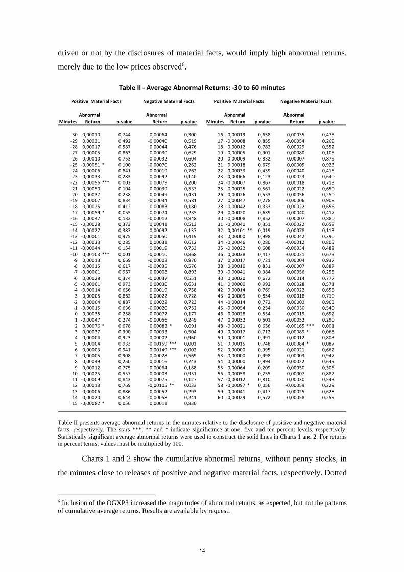
driven or not by the disclosures of material facts, would imply high abnormal returns,

merely due to the low prices observed6.

Table II presents average abnormal returns in the minutes relative to the disclosure of positive and negative material facts, respectively. The stars ***, ** and * indicate significance at one, five and ten percent levels, respectively. Statistically significant average abnormal returns were used to construct the solid lines in Charts 1 and 2. For returns in percent terms, values must be multiplied by 100.

Charts 1 and 2 show the cumulative abnormal returns, without penny stocks, in

the minutes close to releases of positive and negative material facts, respectively. Dotted

6 Inclusion of the OGXP3 increased the magnitudes of abnormal returns, as expected, but not the patterns of cumulative average returns. Results are available by request.

Abnormal Abnormal Abnormal Abnormal

Minutes Return p‐value Return p‐value Minutes Return p‐value Return p‐value

‐30 ‐0,00010 0,744 ‐0,00064 0,300 16 ‐0,00019 0,658 0,00035 0,475‐29 0,00021 0,492 ‐0,00040 0,519 17 ‐0,00008 0,855 ‐0,00054 0,269‐28 0,00017 0,587 0,00044 0,476 18 0,00012 0,782 0,00029 0,552‐27 0,00005 0,863 0,00030 0,629 19 ‐0,00005 0,901 ‐0,00080 0,105‐26 0,00010 0,753 ‐0,00032 0,604 20 0,00009 0,832 0,00007 0,879‐25 ‐0,00051 * 0,100 ‐0,00070 0,262 21 0,00018 0,679 0,00005 0,923‐24 0,00006 0,841 ‐0,00019 0,762 22 ‐0,00033 0,439 ‐0,00040 0,415‐23 ‐0,00033 0,283 0,00092 0,140 23 0,00066 0,123 ‐0,00023 0,640‐22 0,00096 *** 0,002 0,00079 0,200 24 ‐0,00007 0,867 0,00018 0,713‐21 ‐0,00050 0,104 ‐0,00039 0,533 25 0,00025 0,561 ‐0,00022 0,650‐20 ‐0,00037 0,238 ‐0,00049 0,431 26 0,00026 0,553 ‐0,00056 0,250‐19 0,00007 0,834 ‐0,00034 0,581 27 0,00047 0,278 ‐0,00006 0,908‐18 0,00025 0,412 0,00083 0,180 28 ‐0,00042 0,333 ‐0,00022 0,656‐17 ‐0,00059 * 0,055 ‐0,00074 0,235 29 0,00020 0,639 ‐0,00040 0,417‐16 0,00047 0,132 ‐0,00012 0,848 30 ‐0,00008 0,852 0,00007 0,880‐15 ‐0,00028 0,373 0,00041 0,513 31 ‐0,00040 0,351 ‐0,00022 0,658‐14 0,00027 0,387 0,00092 0,137 32 0,00101 ** 0,019 0,00078 0,113‐13 ‐0,00001 0,975 0,00050 0,419 33 0,00000 0,998 ‐0,00042 0,390‐12 0,00033 0,285 0,00031 0,612 34 ‐0,00046 0,280 ‐0,00012 0,805‐11 ‐0,00044 0,154 0,00019 0,753 35 ‐0,00022 0,608 ‐0,00034 0,482‐10 0,00103 *** 0,001 ‐0,00010 0,868 36 0,00038 0,417 ‐0,00021 0,673‐9 0,00013 0,669 ‐0,00002 0,970 37 0,00017 0,721 0,00004 0,937‐8 0,00015 0,617 ‐0,00035 0,576 38 0,00010 0,831 ‐0,00007 0,887‐7 ‐0,00001 0,967 0,00008 0,893 39 ‐0,00041 0,384 0,00056 0,255‐6 0,00028 0,374 ‐0,00037 0,551 40 0,00020 0,672 0,00014 0,777‐5 ‐0,00001 0,973 0,00030 0,631 41 0,00000 0,992 0,00028 0,571‐4 ‐0,00014 0,656 0,00019 0,758 42 0,00014 0,769 ‐0,00022 0,656‐3 ‐0,00005 0,862 ‐0,00022 0,728 43 ‐0,00009 0,854 ‐0,00018 0,710‐2 0,00004 0,887 0,00022 0,723 44 ‐0,00014 0,772 0,00002 0,963‐1 ‐0,00015 0,636 ‐0,00020 0,752 45 ‐0,00054 0,254 0,00030 0,5400 0,00035 0,258 ‐0,00077 0,177 46 0,00028 0,554 ‐0,00019 0,6921 ‐0,00047 0,274 ‐0,00056 0,249 47 0,00032 0,501 ‐0,00052 0,2902 0,00076 * 0,078 0,00083 * 0,091 48 ‐0,00021 0,656 ‐0,00165 *** 0,0013 0,00037 0,390 ‐0,00033 0,504 49 0,00017 0,712 0,00089 * 0,0684 0,00004 0,923 0,00002 0,960 50 0,00001 0,991 0,00012 0,8035 0,00004 0,933 ‐0,00159 *** 0,001 51 0,00015 0,748 ‐0,00084 * 0,0876 0,00003 0,941 0,00149 *** 0,002 52 0,00000 0,995 ‐0,00021 0,6627 ‐0,00005 0,908 0,00028 0,569 53 0,00000 0,998 0,00003 0,9478 0,00049 0,250 0,00016 0,743 54 0,00000 0,994 ‐0,00022 0,6499 0,00012 0,775 0,00064 0,188 55 0,00064 0,209 0,00050 0,306

10 ‐0,00025 0,557 ‐0,00003 0,951 56 ‐0,00058 0,255 0,00007 0,88211 ‐0,00009 0,843 ‐0,00075 0,127 57 ‐0,00012 0,810 0,00030 0,54312 0,00013 0,769 ‐0,00105 ** 0,033 58 ‐0,00097 * 0,056 ‐0,00059 0,22913 ‐0,00006 0,886 0,00052 0,293 59 0,00041 0,417 0,00025 0,62814 0,00020 0,644 ‐0,00058 0,241 60 ‐0,00029 0,572 ‐0,00058 0,25915 ‐0,00082 * 0,056 0,00011 0,830

Table II ‐ Average Abnormal Returns: ‐30 to 60 minutes

Negative Material Facts Negative Material FactsPositive Material Facts Positive Material Facts

14

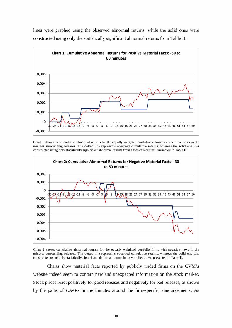
lines were graphed using the observed abnormal returns, while the solid ones were

constructed using only the statistically significant abnormal returns from Table II.

Chart 1 shows the cumulative abnormal returns for the equally weighted portfolio of firms with positive news in the minutes surrounding releases. The dotted line represents observed cumulative returns, whereas the solid one was constructed using only statistically significant abnormal returns from a two-tailed t-test, presented in Table II.

Chart 2 shows cumulative abnormal returns for the equally weighted portfolio firms with negative news in the minutes surrounding releases. The dotted line represents observed cumulative returns, whereas the solid one was constructed using only statistically significant abnormal returns in a two-tailed t-test, presented in Table II.

Charts show material facts reported by publicly traded firms on the CVM’s

website indeed seem to contain new and unexpected information on the stock market.

Stock prices react positively for good releases and negatively for bad releases, as shown

by the paths of CAARs in the minutes around the firm-specific announcements. As

‐0,001

0

0,001

0,002

0,003

0,004

0,005

‐30 ‐27 ‐24 ‐21 ‐18 ‐15 ‐12 ‐9 ‐6 ‐3 0 3 6 9 12 15 18 21 24 27 30 33 36 39 42 45 48 51 54 57 60

Chart 1: Cumulative Abnormal Returns for Positive Material Facts: ‐30 to 60 minutes

‐0,006

‐0,005

‐0,004

‐0,003

‐0,002

‐0,001

0

0,001

0,002

‐30 ‐27 ‐24 ‐21 ‐18 ‐15 ‐12 ‐9 ‐6 ‐3 0 3 6 9 12 15 18 21 24 27 30 33 36 39 42 45 48 51 54 57 60

Chart 2: Cumulative Abnormal Returns for Negative Material Facts: ‐30 to 60 minutes

15

reported in prior studies on market efficiency, our findings indicate price adjustments to

market news are not instantaneous. After good and bad news, graphs above show stock

prices take about thirty and fifty minutes to estabilize, respectively, with an earlier

stabilization for the good news portfolio. This last result is consistent with the higher

costs associated with short selling operations. Furthermore, during the whole period,

stock returns changed substantially, without evidence of overreaction in stock prices.

Considering the statistically significant returns, cumulative returns for positive

(negative) news changed from zero to 0.23% (-0.35%). The magnitudes of stock price

reactions and the speed of price response reveal profit opportunities for those market

participants who trade in the minutes close to the release of material facts in Brazil.

Additionally, given that our sample comprised only liquid stocks traded in

BM&FBOVESPA, perhaps our results hint at the lowest time needed for stock prices to

completely incorporate new information in Brazil.

Actually, while stock returns started reacting to bad news just after releases,

cumulative returns for the portfolio of firms with good news started to rise about

twenty-four minutes prior to disclosures, suggesting anticipated trading activity. Adding

up average returns before positive facts, we found 0.14%. Thus, for positive material

news, it seems that some price adjustments took place before the announcements. On

this issue, we should stress the possibility of firms disclosing material facts just after

unusual price reactions or trading activity, following CVM’s specific recommendations

precisely stated to avoid insider trading. In this case, we could be observing firms’

announcements reacting to prices, instead of the opposite. Nevertheless, this type of

reversal causality does not change our conclusions hinting at insider trading.

Aiming to ensure robustness to the results we found using the market model and

the CAPM, we used a control group as an alternative benchmark to calculate abnormal

returns. The control firms belong to the same industry of the treated firms, i.e., those

whose material facts were disclosed during the trading time. A robustness test of this

type is important since industry-specific shocks may increase the differences between

observed returns and expected returns calculated from market-based models. Matching

for industry was employed by Busse and Green (2002), Hendricks and Singhal (2001)

and Womack (1996) to control industry-specific effects on stock returns. In selecting

companies for the control group we relied on a classification by industry prepared by

the BMF&BOVESPA, available on the institution’s website and developed to provide a

16

clearer view of the areas of activity of the listed companies to investors. This

classification was built considering mainly the types and uses of the products and

services developed by listed companies. Following this grouping by industry, we identified

for each company in our sample a set of firms that (i) belong to the same industry and (ii)

meet the liquidity criterion previously set7. Abnormal returns from this approach were

computed as follows:

, , _ , (2)

In equation (2), AR , and R , represent, respectively, abnormal and observed

returns of stock i in transaction t, while R _ , is the return in transaction t of an equally

weighted portfolio of firms from the same industry as firm i. In the case where we could

not identify firms that met the liquidity criterion, R _ , was replaced by R , , the return

of the Ibovespa index. After having calculated the abnormal returns for each company,

we computed the average returns for the companies that reported positive material facts

, and for the corresponding control firms _ , ). After that, we applied t-tests to

identify statistically significant differences between the averages , and _ , , i.e.,

statistically significant average abnormal returns. Standard deviation estimates of this

difference were computed from the empirical distributions of , and _ , . The

booststrap method set previously was applied to construct the empirical distributions.

We applied the same procedure for negative material facts. Table III shows average

abnormal returns from -30 to 60 minutes and p-values of a two-tailed t-test for both

positive and negative material facts.

7 We identified controls for the following companies: Eletropaulo (Cemig, Cesp, Copel, CPFL, Light, and Tractebel), Anhanguera (Kroton and Estacio Participações), Banco do Brasil (Banrisul, Bradesco, Itaú, and Santander), Brookfield (Even, Eztec, MRV, JHSF, PDG, Rossi, Tecnisa, Direcional, Cyrella, and Gafisa), Gafisa (Even, Eztec, MRV, JHSF, PDG, Rossi, Tecnisa, Direcional, Cyrella, and Brookfield), CPFL (Cemig, Cesp, Copel, Eletropaulo, Light, and Tractebel), Odontoprev (Qualicorp), Santander (Banco do Brasil, Banrisul, Bradesco, and Itaú), MMX (Vale do Rio Doce), HRT (Petrobras), Ecorodovias (CCR), and Vale do Rio Doce (MMX). For the remaining companies we used the Ibovespa index.

17

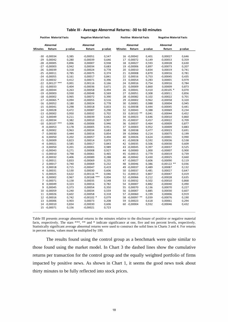
Table III presents average abnormal returns in the minutes relative to the disclosure of positive or negative material facts, respectively. The stars ***, ** and * indicate significance at one, five and ten percent levels, respectively. Statistically significant average abnormal returns were used to construct the solid lines in Charts 3 and 4. For returns in percent terms, values must be multiplied by 100.

The results found using the control group as a benchmark were quite similar to

those found using the market model. In Chart 3 the dashed lines show the cumulative

returns per transaction for the control group and the equally weighted portfolio of firms

impacted by positive news. As shown in Chart 1, it seems the good news took about

thirty minutes to be fully reflected into stock prices.



‐30 ‐0,00034 0,385 ‐0,00051 0,547 16 ‐0,00042 0,401 0,00027 0,646‐29 0,00042 0,280 ‐0,00039 0,646 17 ‐0,00072 0,149 ‐0,00053 0,359‐28 ‐0,00005 0,896 0,00007 0,938 18 0,00027 0,593 0,00028 0,630‐27 ‐0,00003 0,942 0,00034 0,683 19 ‐0,00006 0,897 ‐0,00073 0,207‐26 0,00039 0,318 ‐0,00024 0,778 20 0,00010 0,834 0,00019 0,741‐25 ‐0,00011 0,785 ‐0,00075 0,374 21 0,00008 0,870 0,00016 0,781‐24 ‐0,00055 0,161 0,00017 0,841 22 0,00016 0,753 ‐0,00045 0,435‐23 ‐0,00032 0,412 0,00071 0,396 23 0,00054 0,283 0,00001 0,979‐22 0,00127 *** 0,001 0,00116 0,166 24 0,00016 0,754 0,00016 0,784‐21 ‐0,00033 0,404 ‐0,00036 0,671 25 0,00009 0,860 0,00009 0,873‐20 ‐0,00044 0,263 ‐0,00058 0,494 26 0,00041 0,410 ‐0,00105 * 0,070‐19 ‐0,00003 0,930 ‐0,00048 0,569 27 0,00051 0,308 ‐0,00011 0,856‐18 ‐0,00002 0,965 0,00072 0,390 28 ‐0,00082 0,102 ‐0,00022 0,701‐17 ‐0,00065 * 0,094 ‐0,00055 0,516 29 ‐0,00002 0,962 ‐0,00058 0,320‐16 0,00052 0,180 0,00024 0,778 30 0,00001 0,988 0,00004 0,945‐15 ‐0,00041 0,298 0,00018 0,833 31 ‐0,00038 0,444 ‐0,00045 0,441‐14 0,00028 0,472 0,00087 0,298 32 0,00043 0,388 0,00069 0,234‐13 ‐0,00002 0,950 0,00032 0,702 33 0,00102 ** 0,041 ‐0,00044 0,452‐12 0,00049 0,211 0,00039 0,642 34 ‐0,00023 0,646 ‐0,00010 0,860‐11 ‐0,00034 0,382 0,00010 0,907 35 ‐0,00037 0,457 ‐0,00022 0,709‐10 0,00107 *** 0,006 ‐0,00006 0,946 36 0,00037 0,464 ‐0,00009 0,877‐9 ‐0,00053 0,178 ‐0,00005 0,951 37 0,00003 0,952 0,00009 0,883‐8 0,00002 0,963 ‐0,00034 0,683 38 0,00038 0,477 ‐0,00023 0,691‐7 0,00030 0,444 0,00016 0,854 39 ‐0,00066 0,214 0,00075 0,199‐6 0,00050 0,202 ‐0,00057 0,494 40 0,00026 0,624 ‐0,00001 0,990‐5 0,00009 0,823 0,00014 0,870 41 ‐0,00028 0,592 0,00036 0,538‐4 0,00021 0,585 0,00017 0,843 42 0,00035 0,506 ‐0,00030 0,609‐3 0,00050 0,201 ‐0,00001 0,989 43 ‐0,00045 0,397 ‐0,00037 0,525‐2 ‐0,00043 0,271 0,00008 0,927 44 0,00000 1,000 ‐0,00007 0,900‐1 ‐0,00010 0,798 ‐0,00061 0,465 45 ‐0,00015 0,779 ‐0,00019 0,7390 ‐0,00032 0,406 ‐0,00089 0,288 46 ‐0,00042 0,430 ‐0,00025 0,6601 ‐0,00011 0,833 ‐0,00069 0,235 47 ‐0,00027 0,606 ‐0,00090 0,1192 0,00017 0,740 0,00069 0,232 48 0,00046 0,386 ‐0,00122 ** 0,0363 0,00018 0,715 ‐0,00047 0,419 49 ‐0,00037 0,489 0,00087 0,1324 0,00031 0,530 0,00030 0,606 50 0,00037 0,481 0,00027 0,6475 ‐0,00025 0,622 ‐0,00116 ** 0,046 51 ‐0,00013 0,807 ‐0,00047 0,4196 0,00002 0,967 0,00168 *** 0,004 52 ‐0,00066 0,212 ‐0,00028 0,6357 ‐0,00071 0,158 0,00035 0,548 53 ‐0,00032 0,502 ‐0,00010 0,8688 0,00049 0,323 0,00016 0,782 54 0,00007 0,882 ‐0,00040 0,4909 0,00045 0,373 0,00054 0,350 55 0,00070 0,136 0,00070 0,227

10 ‐0,00059 0,240 0,00034 0,559 56 0,00007 0,885 0,00030 0,60711 0,00026 0,602 ‐0,00058 0,318 57 ‐0,00060 0,199 0,00006 0,91912 ‐0,00016 0,742 ‐0,00102 * 0,079 58 ‐0,00097 ** 0,039 ‐0,00076 0,19013 0,00006 0,903 0,00073 0,208 59 0,00023 0,618 0,00061 0,29414 ‐0,00010 0,834 ‐0,00030 0,606 60 ‐0,00004 0,932 ‐0,00046 0,43215 ‐0,00071 0,156 ‐0,00021 0,723

Table III ‐ Average Abnormal Returns: ‐30 to 60 minutes


18

Chart 3 shows cumulative returns for the control group and the equally weighted portfolio of firms with positive news in the minutes surrounding releases. The dotted line represents observed cumulative returns, whereas the solid one was constructed using only statistically significant abnormal returns in a two-tailed t-test.

Chart 4 shows the same results for firms that released negative material facts:

Chart 4 shows cumulative returns for the control group and the equally weighted portfolio of firms with negative news in the minutes surrounding releases. The dotted line represents observed cumulative returns, whereas the solid one was constructed using only statistically significant abnormal returns in a two-tailed t-test.

Such cumulative returns were calculated from the price changes of the stocks

comprising each portfolio throughout the period. We should point out that the returns of

the treated firms in the minutes close to the release of material facts were quite notable.

‐0,002

‐0,001

0

0,001

0,002

0,003

0,004

‐30 ‐27 ‐24 ‐21 ‐18 ‐15 ‐12 ‐9 ‐6 ‐3 0 3 6 9 12 15 18 21 24 27 30 33 36 39 42 45 48 51 54 57 60


Treated Group Control Group Abnormal Returns

‐0,007

‐0,006

‐0,005

‐0,004

‐0,003

‐0,002

‐0,001

0,000

0,001

0,002

‐30 ‐26 ‐22 ‐18 ‐14 ‐10 ‐6 ‐2 2 6 10 14 18 22 26 30 34 38 42 46 50 54 58

Chart 4: Cumulative Abnormal Returns for Negative Material Facts: ‐30 to 60 minutes

Treated Group Control Group Abnormal returns

19

The solid line in the diagrams was constructed using the statistically significant

abnormal returns indicated in Table III.

Busse and Green (2002) reported that cumulative returns stabilized at -1.25%

and 0.50%, after the Morning Call negative mentions and Midday Call positive news,

respectively. Although our findings indicate profit opportunities, our rates are

considerably smaller. One possible explanation for this result is that firms in Brazil

usually only disclose information not supposed to cause excessive volatility in prices

during the trading time.

Recently, event studies employing intraday data have shown that prices adjust

quickly to new information. Kim et al. (2007) provides evidence stock prices in the US

stock market take five to fifteen minutes to fully reflect the information contained in

buying recommendations pre-released by analysts before the market opens, arguing

competition among traders causes information to be fully reflected into stock prices.

Similarly, Busse and Green (2002) results pointed out stock prices in the US market

take up to thirteen minutes to impound the new information. Consistent with the results

reported by Drienko and Sault (2013), our findings indicate new information is

incorporated into stock prices within fifty minutes. Yet, this time is longer than that

observed by Kim et al. (1997) and Busse and Green (2002), as expected given the size

and the trading volume in the US stock market. However, it is important to highlight our

conclusions remain aligned with those found in the studies on market efficiency, in the

sense that markets are efficient but offer short-term profit opportunities for those who

follow them more closely.

4.2—Number of Shares Traded

Concerning the traded volume, we performed the Wilcoxon test for medians to

test whether the median number of shares traded in the minutes immediately after and

before releases of material facts were higher than the observed medians in other trading

minutes. For positive material facts, stars in Table IV denote that the median number of

shares traded in the minute indicated by the column is statistically higher than the

median number of shares traded in the minute specified by the row.

Wilcoxon tests for positive news revealed that the medians calculated for the

fourth minute before and for the first minute after disclosures are higher than the

medians computed for a number of minutes before the announcements. The number of

20

shares traded increased in the first minute after the release of positive news, indicating

that market participants indeed seek to exploit profit opportunities. To the extent that the

median number of shares traded also grew four minutes before the disclosure of good

news, the results again hint at some anticipated trading activity.

Table IV presents the median number of traded shares in the minutes relative to the disclosure of positive news. Wilcoxon statistics are shown in parentheses. Two and three stars mean the median number of shares traded in the minute indicated by the column is statistically higher than the median number of shares traded in the minute specified by the row, at five and one percent levels, respectively. Tests were performed from -10 to 10 minutes relative to disclosures.

Table V shows the results of the Wilcoxon’s test for negative material facts.

Compared to the case of positive news, we found weaker evidence of changes in the

number of shares traded. Nonetheless, we detected increases in the amounts traded, at a

significance level of 5%, in the ninth minute following the disclosure of negative news.

The high number of shares traded was associated with decreases in stock returns.

‐5 to ‐10 ‐4 ‐3 ‐2 ‐1 0 1 2‐10

0 to ‐5

‐6

‐7 5200 (1,82)** 4300 (2,09)**

‐8 4300 (1,65)**

‐9

‐10 4300 (2,09)**

‐11

‐12

‐13

‐14

‐15 5200 (1,89)** 4600 (1,68)** 4300 (2,36)***

‐16

‐17 4300 (1,94)**

‐18 5200 (1,66)** 4300 (1,67)**

‐19 5200 (1,92)**

‐20 5200 (1,76)** 4300 (2,21)**

surrounding disclosures of positive news

Table IV ‐ Wilcoxon test for the number of shares traded in the minutes

21

Table V presents the median number of traded shares in the minutes relative to the disclosure of positive news. Wilcoxon statistics are shown in parentheses. Two and three stars mean the median number of shares traded in the minute indicated by the column is statistically higher than the median number of shares traded in the minute specified by the row, at five and one percent levels, respectively. Tests were performed from -10 to 10 minutes relative to disclosures.

5. Conclusion

In this paper we used intraday stock returns and compulsory releases of material

facts by publicly traded companies to assess market efficiency in Brazil. Our event

study coupled a high-frequency database on transaction prices and traded volume with a

set of material facts provided by the regulatory authority of security markets in Brazil in

order to evaluate how fast stock prices fully reflect all information made publicly

available. We believe the main contribution of this paper is to produce some evidence

on market efficiency in Brazil using intraday data on stock prices, traded shares, and the

releasing of material facts.

According to our results, material facts reported by publicly traded firms indeed

seem to reveal new and unexpected information to the stock market. Price adjustments

to news are not instantaneous, as reported in prior event studies using intraday data. Our

results pointed out stock prices in Brazil take up to fifty minutes to incorporate the

news.

During the entire period of price adjustments, stock returns changed

substantially. Cumulative returns for positive news changed in approximately 0.23 p.p.

from twenty-four minutes before to thirty-three minutes after disclosures. For negative

material news, cumulative returns decreased 0.35 p.p. after fifty minutes. The

magnitudes of stock price reactions and the speed of price response reveal profit

‐2 to ‐10 0 5 6 7 8 9 10

0 to ‐5

‐6

‐7 4100 (1,33)* 8000 (1,41)*

‐8 8000 (1,39)*

‐9 4500 (1,28)* 4100 (1,46)* 8000 (1,80)**

‐10

‐11

‐12

‐13 8000 (1,66)**

‐14

‐15 to ‐20

Table V ‐ Wilcoxon test for the number of shares traded in the minutes

surrounding disclosures of negative news

22

opportunities for those market participants who trade in the minutes close to the release

of material facts in Brazil. Our results are robust for penny stocks. Similar results were

also found using a control group of firms as an alternative benchmark.

The number of shares traded increased in the first minute after the release of

positive news, and in the ninth minute after the release of negative material news,

indicating that market participants indeed react to profit opportunities. Because we

observed price reactions prior to the disclosure of material facts and a high median

number of shares traded four minutes before the release of good news, our results also

hint at some anticipated trading activity.

23

References [1] Atkins, A.B., Dyl, E. Price reversals, bid–ask spreads, and market efficiency. Journal of Financial and Quantitative Analysis, 25, pp. 535–547, 1990. [2] Ball, Ray. The Theory of Stock Market Efficiency: Acomplishments and Limitations. In The New Corporate Finance, edited by Donald H. Chew, Jr. McGraw-Hil Irwin, third edition, 1994. [3] Barclay, Michael J.; Litzenberger, Robert H. Announcements Effects of New Equity Issues and the Use of Intraday Price Data. Journal of Financial Economics 21, pp. 71-89, 1988. [4] Busse, Jeffrey A,; Green, T. Clifton. Market Efficiency in Real Time. Journal of Financial Economics 65, pp. 415-437, 2002. [5] Campbell, John Y; Lo, Andrew W.; MacKinlay, Craig A. The Econometrics of Financial Markets. Princeton University Press, 1997. [6] Drienko, J.; Sault, Stephen J. The intraday Impact of company responses to exchange queries. Journal of Banking &Finance 37, 2013. [7] Fama, Eugene F.; Fischer, Lawrence; Jensen, Michael C.; Roll, Richard. The Adjustment of Stock Prices to New Information. International Economic Review 10, 1969. [8] Fama, Eugene F. Efficient Capital Markets: A Review of Theory and Empirical Work. Journal of Finance 25, vol. 2, pp. 383-417, 1970. [9] Faust, J.; Rogers, H.J.; Wang, S.B.; and Wright H.J. The High Frequency Response of Exchange Rates and Interest Rates to Macroeconomic Announcements. Journal of Monetary Economics 54, pp.1051–1068, 2007. [10] Gürkainak, S.R.; Sack, B.; Swanson, T. E. Do Actions Speak Louder Than Words? The Response of Asset Prices to Monetary Policy Actions and Statements. International Journal of Central Banking 1, pp. 55-93, 2005. [11] Hautsch, Nikolaus. Econometrics of Financial High-Frequency Data. Springer, 2012. [12] Hendricks, K.; Singhal, V. The Long-Run Stock Price Performance of Firms with Effective TQM Programs. Management Science 47, pp. 359–368, 2001. [13] Hertzel, M.; Lemmon, M.; Linck, J.; Rees, L. Long-run Performance Following Private Placements of Equity. Journal of Finance 57, pp. 2595–2617, 2002. [14] Kim, S.; Lin, J.; Slovin, M. Market Structure, Informed Trading and Analysts’ Recommendations. Journal of Financial and Quantitative Analysis 32, pp. 507-524, 1997.

24

[15] Krishnan, R.; Mishra, V. Intraday Liquidity Patterns in India Stock Market. Journal of Asian Economics 28, pp. 99-104, 2013. [16] MacKinlay, A.C. Event Studies in Economics and Finance. Journal of Economic Literature.Vol. XXXV, pp. 13-39, 1997. [17] McInish, Thomas H.; Wood, Robert A. An Analysis of Intraday Patterns in Bid/Ask Spreads for NYSE Stocks. The Journal of Finance, Vol. XLVII, No. 2, 1992. [18] Murcia, Flávia C. S.; Murcia, F. D.; Borba, F.A. The Informational Content of Credit Ratings in Brazil: An Event Study. Brazilian Review of Finance, vol. 11, n.4, pp. 503-526, 2013. 19 [19] Patell, J.; Wolfson, M. The Intraday Speed of Adjustment of Stock Prices to Earnings and Dividend Announcements. Journal of Financial Economics 13, pp. 223-252, 1984. [20] Swanson, E.T. Let’s Twist Again: A High-Frequency Event-Study Analysis of Operation Twist and Its Implications for QE2. Brookings Papers on Economic Activity, pp. 151–188, 2011. [21] Womack, K. Do Brokerage Analysts’ Recommendations Have Investment Value? Journal of Finance 51, pp. 137-167, 1996.

25

Appendix I - CAPM Results

Table VI presents average abnormal returns computed from CAPM model in the minutes relative to the disclosure of positive and negative material facts. The stars ***, ** and * indicate significance at one, five and ten percent levels, respectively. Statistically significant average abnormal returns were used to construct the solid lines in Charts 3 and 4. For returns in percent terms, values must be multiplied by 100.



‐30 ‐0,00017 0,600 ‐0,00064 0,254 16 ‐0,00026 0,546 0,00035 0,466‐29 0,00034 0,293 ‐0,00040 0,479 17 0,00000 0,999 ‐0,00054 0,264‐28 0,00017 0,592 0,00044 0,429 18 0,00013 0,769 0,00029 0,544‐27 0,00007 0,820 0,00030 0,590 19 ‐0,00001 0,989 ‐0,00079 * 0,100‐26 0,00010 0,751 ‐0,00032 0,570 20 0,00009 0,843 0,00008 0,874‐25 ‐0,00047 0,146 ‐0,00069 0,217 21 0,00014 0,756 0,00005 0,918‐24 0,00019 0,557 ‐0,00018 0,742 22 ‐0,00040 0,362 ‐0,00040 0,411‐23 ‐0,00042 0,191 0,00092 0,102 23 0,00073 * 0,092 ‐0,00023 0,639‐22 0,00090 *** 0,005 0,00080 0,155 24 ‐0,00020 0,649 0,00018 0,706‐21 ‐0,00053 * 0,098 ‐0,00038 0,493 25 0,00032 0,464 ‐0,00022 0,649‐20 ‐0,00047 0,141 ‐0,00049 0,386 26 0,00033 0,445 ‐0,00056 0,245‐19 0,00022 0,491 ‐0,00034 0,545 27 0,00044 0,316 ‐0,00005 0,910‐18 0,00011 0,742 0,00083 0,137 28 ‐0,00034 0,439 ‐0,00022 0,654‐17 ‐0,00054 * 0,090 ‐0,00073 0,191 29 0,00025 0,571 ‐0,00040 0,413‐16 0,00031 0,332 ‐0,00012 0,836 30 ‐0,00002 0,957 0,00008 0,875‐15 ‐0,00024 0,451 0,00041 0,466 31 ‐0,00040 0,361 ‐0,00021 0,656‐14 0,00021 0,520 0,00092 * 0,099 32 0,00099 ** 0,022 0,00078 0,106‐13 0,00006 0,862 0,00050 0,369 33 ‐0,00002 0,961 ‐0,00042 0,386‐12 0,00035 0,280 0,00032 0,572 34 ‐0,00041 0,348 ‐0,00012 0,806‐11 ‐0,00058 * 0,072 0,00020 0,725 35 ‐0,00020 0,651 ‐0,00034 0,478‐10 0,00106 *** 0,001 ‐0,00010 0,858 36 0,00024 0,583 ‐0,00020 0,672‐9 0,00006 0,862 ‐0,00002 0,971 37 0,00027 0,530 0,00004 0,932‐8 0,00024 0,458 ‐0,00034 0,540 38 0,00009 0,831 ‐0,00007 0,889‐7 ‐0,00003 0,914 0,00009 0,878 39 ‐0,00030 0,490 0,00056 0,246‐6 0,00010 0,746 ‐0,00037 0,513 40 0,00011 0,801 0,00014 0,770‐5 0,00002 0,942 0,00030 0,592 41 0,00003 0,952 0,00028 0,562‐4 ‐0,00011 0,731 0,00019 0,730 42 0,00010 0,824 ‐0,00022 0,654‐3 ‐0,00008 0,810 ‐0,00021 0,704 43 0,00003 0,945 ‐0,00018 0,710‐2 ‐0,00003 0,917 0,00007 0,899 44 ‐0,00013 0,763 0,00002 0,959‐1 ‐0,00015 0,630 0,00039 0,488 45 ‐0,00043 0,318 0,00030 0,5320 0,00026 0,420 ‐0,00077 0,153 46 0,00028 0,515 ‐0,00019 0,6911 ‐0,00045 0,302 ‐0,00056 0,244 47 0,00032 0,460 ‐0,00052 0,2852 0,00075 * 0,085 0,00083 * 0,086 48 ‐0,00042 0,331 ‐0,00165 *** 0,0013 0,00034 0,429 ‐0,00032 0,501 49 0,00036 0,414 0,00090 * 0,0634 ‐0,00005 0,915 0,00003 0,956 50 0,00000 0,992 0,00012 0,7965 0,00011 0,795 ‐0,00159 *** 0,001 51 0,00015 0,732 ‐0,00084 * 0,0836 0,00004 0,919 0,00150 *** 0,002 52 0,00006 0,889 ‐0,00021 0,6607 ‐0,00002 0,966 0,00028 0,561 53 ‐0,00005 0,927 0,00003 0,9428 0,00051 0,242 0,00016 0,736 54 0,00000 0,997 ‐0,00022 0,6479 0,00015 0,734 0,00065 0,181 55 0,00065 0,184 0,00050 0,297

10 ‐0,00033 0,450 ‐0,00003 0,953 56 ‐0,00050 0,310 0,00007 0,87711 ‐0,00010 0,819 ‐0,00075 0,123 57 ‐0,00012 0,807 0,00030 0,53412 0,00011 0,799 ‐0,00104 ** 0,031 58 ‐0,00106 ** 0,031 ‐0,00059 0,22413 ‐0,00010 0,821 0,00052 0,284 59 0,00049 0,320 0,00025 0,60414 0,00016 0,705 ‐0,00057 0,236 60 ‐0,00022 0,656 ‐0,00057 0,23515 ‐0,00075 * 0,084 0,00011 0,824

Table VI ‐ Average Abnormal Returns: ‐30 to 60 minutes ‐ CAPM


26

II - CAPM – Cumulative Abnormal Returns

Chart 5 shows cumulative abnormal returns for the equally weighted portfolio of firms with positive news in the minutes surrounding the releases, computed from the CAPM model. The dotted line represents observed cumulative returns whereas the solid one was constructed using only statistically significant abnormal returns in a two-tailed t test, presented in Table IV.

Chart 6 shows cumulative abnormal returns for the equally weighted portfolio of firms with negative news in the minutes surrounding the releases, computed from the CAPM model. The dotted line represents observed cumulative returns whereas the solid one was constructed using only statistically significant abnormal returns in a two-tailed t test, presented in Table IV.

‐0,001

0

0,001

0,002

0,003

0,004

0,005

‐30 ‐27 ‐24 ‐21 ‐18 ‐15 ‐12 ‐9 ‐6 ‐3 0 3 6 9 12 15 18 21 24 27 30 33 36 39 42 45 48 51 54 57 60


‐0,006

‐0,005

‐0,004

‐0,003

‐0,002

‐0,001

0,000

0,001

0,002

0,003

‐30 ‐27 ‐24 ‐21 ‐18 ‐15 ‐12 ‐9 ‐6 ‐3 0 3 6 9 12 15 18 21 24 27 30 33 36 39 42 45 48 51 54 57 60


27

III ‐ Market Model – Firms’ Abnormal Returns Positive Material Facts:

‐0,0050

0,0000

0,0050

0,0100

0,0150

0,0200

‐30 ‐26 ‐22 ‐18 ‐14 ‐10 ‐6 ‐2 2 6 10 14 18 22 26 30 34 38 42 46 50 54 58

VALE4 ‐ 03/11/2013 12:43h

0,0000

0,0020

0,0040

0,0060

0,0080

0,0100

0,0120

0,0140

‐30 ‐26 ‐22 ‐18 ‐14 ‐10 ‐6 ‐2 2 6 10 14 18 22 26 30 34 38 42 46 50 54 58

VALE4 ‐ 11/11/13 13:40h

‐0,0150

‐0,0100

‐0,0050

0,0000

0,0050

0,0100

1 3 5 7 9 11 13 15 17 19 21 23 25 27 29 31 33 35 37 39 41 43 45 47 49 51 53 55 57 59

CPFE ‐ 07/08/13 10:00h

‐0,0020

0,0000

0,0020

0,0040

0,0060

0,0080

0,0100

0,0120

0,0140

0,0160

‐30 ‐26 ‐22 ‐18 ‐14 ‐10 ‐6 ‐2 2 6 10 14 18 22 26 30 34 38 42 46 50 54 58

ECOR3 ‐ 04/17/2013 12:47h

‐0,0020

0,0000

0,0020

0,0040

0,0060

0,0080

0,0100

0,0120

0,0140

‐30 ‐26 ‐22 ‐18 ‐14 ‐10 ‐6 ‐2 2 6 10 14 18 22 26 30 34 38 42 46 50 54 58

ELPL ‐ 07/03/13 15:03h

‐0,0300

‐0,0250

‐0,0200

‐0,0150

‐0,0100

‐0,0050

0,0000

0,0050

0,0100

1 3 5 7 9 11 13 15 17 19 21 23 25 27 29 31 33 35 37 39 41 43 45 47 49 51 53 55 57 59

MMX3 ‐ 09/10/13 10:01h

‐0,0100

‐0,0090

‐0,0080

‐0,0070

‐0,0060

‐0,0050

‐0,0040

‐0,0030

‐0,0020

‐0,0010

0,0000‐30 ‐26 ‐22 ‐18 ‐14 ‐10 ‐6 ‐2 2 6 10 14 18 22 26 30 34 38 42 46 50 54 58

ODPV3‐08/05/13 10:36h

‐0,0030

‐0,0020

‐0,0010

0,0000

0,0010

0,0020

0,0030

0,0040

0,0050

0,0060

‐30 ‐26 ‐22 ‐18 ‐14 ‐10 ‐6 ‐2 2 6 10 14 18 22 26 30 34 38 42 46 50 54 58

PCAR I ‐ 04/17/13 13:01h

‐0,0040

‐0,0030

‐0,0020

‐0,0010

0,0000

0,0010

0,0020

0,0030

0,0040

‐30 ‐27 ‐24 ‐21 ‐18 ‐15 ‐12 ‐9 ‐6 ‐3 0 3 6 9 12 15 18 21 24 27 30 33

PCAR4 ‐ 10/18/13 16:06h

‐0,007

‐0,006

‐0,005

‐0,004

‐0,003

‐0,002

‐0,001

0

0,001

0,002

‐30 ‐26 ‐22 ‐18 ‐14 ‐10 ‐6 ‐2 2 6 10 14 18 22 26 30 34 38 42 46 50 54 58

AEDU3 ‐ 04/23/13 ‐ 11:01h

28

‐0,0030

‐0,0020

‐0,0010

0,0000

0,0010

0,0020

0,0030

0,0040

1 3 5 7 9 11 13 15 17 19 21 23 25 27 29 31 33 35 37 39 41 43 45 47 49 51 53 55 57 59

VALE4 ‐ 11/14/13 10:00h

‐0,0050

‐0,0040

‐0,0030

‐0,0020

‐0,0010

0,0000

0,0010

0,0020

‐30

‐27

‐24

‐21

‐18

‐15

‐12 ‐9 ‐6 ‐3 0 3 6 9

12

15

18

21

24

27

30

33

36

39

42

45

48

51

VALE4 ‐ 12/20/13 14:16h

‐0,0010

0,0000

0,0010

0,0020

0,0030

0,0040

0,0050

‐30 ‐26 ‐22 ‐18 ‐14 ‐10 ‐6 ‐2 2 6 10 14 18 22 26 30 34 38 42 46 50 54 58

VALE4 ‐ 12/26/13 11:48h

‐0,0070

‐0,0060

‐0,0050

‐0,0040

‐0,0030

‐0,0020

‐0,0010

0,0000

0,0010

0,0020

‐30 ‐26 ‐22 ‐18 ‐14 ‐10 ‐6 ‐2 2 6 10 14 18 22 26 30 34 38 42 46 50 54 58

VALE4 ‐ 12/27/13 16:00h

‐0,0080

‐0,0060

‐0,0040

‐0,0020

0,0000

0,0020

0,0040

‐30 ‐26 ‐22 ‐18 ‐14 ‐10 ‐6 ‐2 2 6 10 14 18 22 26 30 34 38 42 46 50 54 58

BBAS3 ‐ 02/03/14 11:58h

‐0,0150

‐0,0100

‐0,0050

0,0000

0,0050

0,0100

0,0150

‐30 ‐26 ‐22 ‐18 ‐14 ‐10 ‐6 ‐2 2 6 10 14 18 22 26 30 34 38 42 46 50 54 58

ESTC3 ‐ 01/20/14 10:58h

‐0,0020

‐0,0010

0,0000

0,0010

0,0020

0,0030

0,0040

0,0050

0,0060

0,0070

‐30 ‐26 ‐22 ‐18 ‐14 ‐10 ‐6 ‐2 2 6 10 14 18 22 26 30 34 38 42 46 50 54 58

KLBN4 ‐ 12/10/13 14:51h

29

Market Model – Firms’ Abnormal Returns Negative Material Facts:

‐0,0050

‐0,0040

‐0,0030

‐0,0020

‐0,0010

0,0000

0,0010

0,0020

0,0030

0,0040

‐30 ‐26 ‐22 ‐18 ‐14 ‐10 ‐6 ‐2 2 6 10 14 18 22 26 30 34 38 42 46 50 54 58

VALE4 ‐ 09/18/13 12:05h

‐0,0020

0,0000

0,0020

0,0040

0,0060

0,0080

0,0100

0,0120

0,0140

0,0160

0,0180

‐30 ‐26 ‐22 ‐18 ‐14 ‐10 ‐6 ‐2 2 6 10 14 18 22 26 30 34 38 42 46 50 54 58

BBAS3 ‐ 04/16/13 16:16h

‐0,0050

‐0,0040

‐0,0030

‐0,0020

‐0,0010

0,0000

0,0010

0,0020

0,0030

0,0040

‐30 ‐26 ‐22 ‐18 ‐14 ‐10 ‐6 ‐2 2 6 10 14 18 22 26 30 34 38 42 46 50 54 58

CPFE ‐ 11/07/13 11:18h

‐0,0200

‐0,0150

‐0,0100

‐0,0050

0,0000

0,0050

‐2 0 2 4 6 8 1012141618202224262830323436384042444648505254565860

GFSA3 ‐ 08/23/13 10:03h

‐0,0100

‐0,0050

0,0000

0,0050

0,0100

0,0150

0,0200

‐30 ‐26 ‐22 ‐18 ‐14 ‐10 ‐6 ‐2 2 6 10 14 18 22 26 30 34 38 42 46 50 54 58

GOLL4 ‐ 04/26/13 15:31h

‐0,0050

‐0,0040

‐0,0030

‐0,0020

‐0,0010

0,0000

0,0010

0,0020

0,0030

0,0040

‐30 ‐26 ‐22‐18‐14‐10 ‐6 ‐2 2 6 10 14 18 22 26 30 34 38 42 46 50 54 58

GOLL4 ‐ 08/04/13 16:27h

‐0,0700

‐0,0600

‐0,0500

‐0,0400

‐0,0300

‐0,0200

‐0,0100

0,0000

0,0100

1 3 5 7 9 11 13 15 17 19 21 23 25 27 29 31 33 35 37 39 41 43 45 47 49 51 53 55 57 59

HRT ‐ 05/13/13 10:01h

‐0,0050

‐0,0040

‐0,0030

‐0,0020

‐0,0010

0,0000

0,0010

0,0020

0,0030

‐30 ‐26 ‐22 ‐18 ‐14 ‐10 ‐6 ‐2 2 6 10 14 18 22 26 30 34 38 42 46 50 54 58

PCAR4 ‐ 05/13/13 12:12h

‐0,0050

‐0,0040

‐0,0030

‐0,0020

‐0,0010

0,0000

0,0010

0,0020

0,0030

0,0040

0,0050

0 2 4 6 8 10 12 14 16 18 20 22 24 26 28 30 32 34 36 38 40 42 44 46 48 50 52 54 56 58 60

Santander ‐ 05/27/13 10:02h

‐0,005

‐0,004

‐0,003

‐0,002

‐0,001

0

0,001

0,002

‐30 ‐26 ‐22 ‐18 ‐14 ‐10 ‐6 ‐2 2 6 10 14 18 22 26 30 34 38 42 46 50 54 58

BISA3 ‐ 02/22/13 15:54h

30

‐0,0100

‐0,0090

‐0,0080

‐0,0070

‐0,0060

‐0,0050

‐0,0040

‐0,0030

‐0,0020

‐0,0010

0,00001 3 5 7 9 11 13 15 17 19 21 23 25 27 29 31 33 35 37 39 41 43 45 47 49 51 53 55 57 59

ALLL4 10/10/13 10:39h

‐0,0060

‐0,0040

‐0,0020

0,0000

0,0020

0,0040

0,0060

0,0080

0,0100

‐30 ‐26 ‐22 ‐18 ‐14 ‐10 ‐6 ‐2 2 6 10 14 18 22 26 30 34 38 42 46 50 54 58

ELPL3 12/27/13 10:40h

0,0000

0,0020

0,0040

0,0060

0,0080

0,0100

0,0120

0,0140

0,0160

0,0180

‐11 ‐8 ‐5 ‐2 1 4 7 10 13 16 19 22 25 28 31 34 37 40 43 46 49 52 55 58

ODPV3 ‐ 10/15/13 11:52h

31

alexandre de carvalho, alberto sanyuan suen e felippe gallo … · 2016-05-17 · alexandre de...

Documents