alex smola, director of machine learning, aws/amazon, at mlconf sf 2016

© 2016, Amazon Web Services, Inc. or its Affiliates. All rights reserved.

Alexander Smola

AWS Machine Learning

Personalization and Scalable Deep Learning with MXNET

Outline

• Personalization • Latent Variable Models • User Engagement and Return Times • Deep Recommender Systems

• MXNet • Basic concepts • Launching a cluster in a minute • Imagenet for beginners

Personalization

Latent Variable Models

• Temporal sequence of observations Purchases, likes, app use, e-mails, ad clicks, queries, ratings

• Latent state to explain behavior • Clusters (navigational, informational queries in search) • Topics (interest distributions for users over time) • Kalman Filter (trajectory and location modeling)

Action

Explanation



• Latent state to explain behavior • Clusters (navigational, informational queries in search) • Topics (interest distributions for users over time) • Kalman Filter (trajectory and location modeling)

Action

Explanation

Are the parametric models really true?



• Latent state to explain behavior • Nonparametric model / spectral • Use data to determine shape • Sidestep approximate inference

x

h

ht = f(xt�1, ht�1)

xt = g(xt�1, ht)



• Latent state to explain behavior • Plain deep network = RNN • Deep network with attention = LSTM / GRU …

(learn when to update state, how to read out)

x

h

Long Short Term Memory

x

h

Schmidhuber and Hochreiter, 1998

i

t

= �(Wi

(xt

, h

t

) + b

i

)

f

t

= �(Wf

(xt

, h

t

) + b

f

)

z

t+1 = f

t

· zt

+ i

t

· tanh(Wz

(xt

, h

t

) + b

z

)

o

t

= �(Wo

(xt

, h

t

, z

t+1) + b

o

)

h

t+1 = o

t

· tanh zt+1

Long Short Term Memory

x

h

Schmidhuber and Hochreiter, 1998

(zt+1, ht+1, ot) = LSTM(zt, ht, xt)

Treat it as a black box

User Engagement

9:01 8:55 11:50

12:30 never

next week ?

(app frame toutiao.com)

http://toutiao.com

User Engagement Modeling

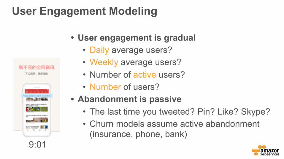
• User engagement is gradual • Daily average users? • Weekly average users? • Number of active users? • Number of users?

• Abandonment is passive • The last time you tweeted? Pin? Like? Skype? • Churn models assume active abandonment

(insurance, phone, bank)9:01

User Engagement Modeling

• User engagement is gradual • Model user returns • Context of activity

• World events (elections, Super Bowl, …) • User habits (morning reader, night owl) • Previous reading behavior

(poor quality content will discourage return)

9:01

Survival Analysis 101

• Model population where something dramatic happens • Cancer patients (death; efficacy of a drug) • Atoms (radioactive decay) • Japanese women (marriage) • Users (opens app)

• Survival probability

IEEE TRANSACTIONS ON KNOWLEDGE AND DATA ENGINEERING, VOL. 100, NO. 10, JANUARY 2016 3

It is well known that the differential equation can be solvedby partial integration, i.e.

Pr(tsurvival � T ) = exp

�Z

T

0�(T )dt

!

. (2)

Hence, if the patient survives until time T and we stopobserving at that point, the likelihood is simply givenby exp

⇣�RT

0 �(T )dt

⌘. This is often referred to as right-

censoring since we observe no further data to the “right”of time T . Moreover, if an event occurs at time t T , thelikelihood is

p(t) = �(t) exp

✓�Z

t

0�(T )dt

◆(3)

Note that there exists a second type of censoring, namelyevents occurring in the interval [0, t0], which denotes aninitial interval during which we do not record times, com-monly referred as left-censoring. While of some theoreticalinterest, this leads to nonconvex optimization problems andmoreover, it does not apply for us, since we have fulldata available without an initial censoring period. We omitdetails accordingly.

In our context the ’death’ event amounts to the usersreturn to the app, and the time of survival amounts to thetime passing until they use the app again.

For any given user with history S

u

= {(bi

, e

i

)} thisamounts to the likelihood:

p(S

u

|T, u) (4)

=

"muY

i=1

�

u

(b

i

)

#

exp

�muX

i=1

Zbi

ei�1

�

u

(t)dt�Z

T

emu

�

u

(t)dt

!

To simplify notation we set e0 = 0. In practice this isreplaced by the first time user u uses the app. By con-struction, the negative log-likelihood is convex in �

u

(t), thepropensity of user u to open the app at time t. Also notethat if we had left censoring, we would have to contendwith 1 � exp

⇣�Rb

0 �

u

(t)dt

⌘. This is not log-concave and

can lead to nontrivial optimization problems. Fortunatelythis problem does not occur in return modeling.

Note that the model is very similar to a Poisson model.The main difference between both models is that we excludethe time interval [b

i

, e

i

] from the analysis until the nextaction. This avoids spurious effects where the app is notopened again since it is already open. While this distinctionmight appear frivolous, it matters when modeling perplex-ities. Hence, rather than a succession of point events wemodel user behavior as a succession of absences and uses ofthe app, where the return timer for event i+1 starts at timee

i

rather than b

i

. This does not complicate the analysis.

3.3 Nonparametric ModelsSo far we did not address the issue of the nonstationaryrate function �

u

(t), governing the propensity of a user toreturn to the app at time t. It is clear that it should take thetime of day, and previous activity of a user into account. Acommon choice, called Hawkes process [28], [29], [30], is toassume that the process is self-exciting. That is, the more auser uses the app, the more likely he is to be using the appagain in the future. This is governed by a so-called trigger

kernel [31], [32] k(t, t0) measuring the effect of behavior attime t0 on events at time t > t

0. It yields the following model:

�

u

(t) =

X

bi<t

k(t, b

i

). (5)

Consequently rate estimation and prediction are trivial,given the kernel k — we simply sum over past events anduse this to predict future activity. Inference of the kernel k isa convex problem and can be accomplished efficiently acrossusers.

Unfortunately such a model lacks the ability to general-ize efficiently across users, to solve cold-start problems or totake the actual activity of a user within the app into account.In particular, it is restricted in a sense that it doesn’t takeusers’ attributes into account. We address these issues in thefollowing section.

4 MODELS

To easily incorporate external features into the model, onesimple choice is the linear function class,

�

u

(t) = h�(u, t), wi (6)

This function class, albeit simple, can be very effective ifwe design the features right. Before we dive into severalpredictors that are subsumed by this framework, we proveequivalence between a model using (5) and a feature-basedapproach.

Lemma 1 Assume that we have a linear feature-based model tocapture the activity and profile of a user. That is, assume that wecan aggregate over past activity via

�(u, t) =

X

i

�(b

i

, e

i

, t) and �

u

(t) = h�(u, t), wi , (7)

where w is the coefficient vector to be estimated. Then this modelis equivalent to a model using trigger kernels, as described in(5). Moreover, any trigger kernel can be decomposed as (7) for asuitable feature map.

Proof: This follows directly by defining a trigger ker-nel k(t, e

i

) := h�(bi

, e

i

, t), wi, i.e. by decomposing �(u, t)

into individual sessions. To prove the converse note thatwe only need a universal kernel [33] since it allows us toapproximate any function in a suitably chosen ReproducingKernel Hilbert Space to arbitrary accuracy.

Now that we have a suitable set of theoretical toolsto analyze user return behavior, we can design practicalmodels that satisfy this purpose. We will use a mix betweenkernel-based and feature based methods. That is, we assumethat

�

u

(t) = h�(u, t), wi+X

bi<t

k(t, b

i

) (8)

We note that despite their equivalence, which we justproved, it’s more clear to write our function class this wayto mix and match between feature-based model and triggerkernels, as it clearly separates the contribution from the twocomponents. The former allows us to add features easily,whereas the latter effectively provides a nonparametric ap-proach to activity estimation. We now have the freedom to

hazard rate function

Session Model

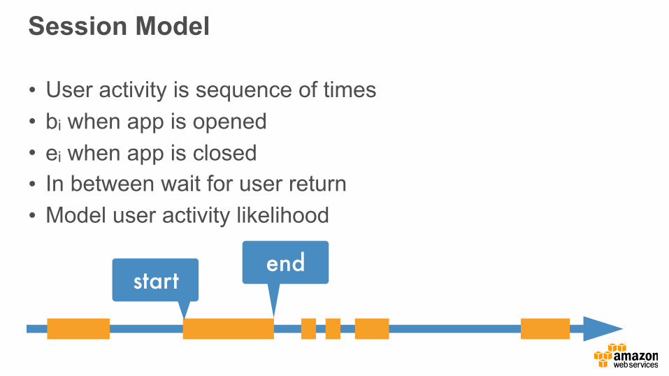
• User activity is sequence of times • bi when app is opened • ei when app is closed • In between wait for user return • Model user activity likelihood

startend


Look up table

One-hot UserID

Hidden2

Hidden1

UserEmbedding

Look up table

One-hot TimeID

TimeEmbedding

……

0 0 1 0 0 0 ……

……

0 0 0 1 0 0 ……

……

……

……

ExternalFeature

Rate

Fig. 1. A Personalized Time-Aware architecture for Survival Analysis.Given the data from previous session, we aims to predict the (quantized)rate values for the next session.

we let the model figure out how time and date shouldcontribute to the predictions. For this purpose we assignan id to each input time slot, quantized by 30 minutes. Thatis, we enumerate the m

T

= 2 · 24 · 7 = 336 segments bybinary indicators. We then introduce another lookup tableB 2 RD⇥mT that projects the one-hot time slot vector to alow dimensional embedding and feed to the DNN, similarto what we did for users. Note that the temporal quantiza-tion only implies that the rate function is piecewise constant,not that we effectively bin the times for the purpose ofsurvival analysis.

Our approach is very similar to the word2vec embed-dings used by [38], albeit with time segments rather thanwords. The idea is that by giving the model enough data, itwill automatically pick up the fact that a Saturday midnighttime slot is different from a Monday morning time slot. Notethat 336 segments are a rather modest choice compared toNLP models, where the space of words may exceed 10,000quite easily.

5.3 Personalized Networks

To learn a personalized and time-aware model, we simplyaggregate the two versions of networks described above, byconcatenating the two embedding vectors as the input to aDeep Network. The idea is that we will be able to learn thepersonalized future rate distribution for a user u, if she quitsthe app at some time slot s.

As before, adding external features is relatively straight-forward in this framework. Again, let x

u

(t) be the featureof user u at time t, we incorporate that by concatenatingx

u

(t) to that of the user and time slot embedding. We showa graphical representation of such a model in Fig. 1.

In a nutshell, the principal difference between the linearmodel discussed before and the models here is that we allowfor a highly nonlinear dependence between attributes, pastobservations, and the rate function, as estimated by themodel. All the above, however, is missing one last crucialcomponent — the ability to reason about the current stateof the model via a latent-variable autoregressive process.We address this via Long Short Term Memory, as describedbelow.

5.4 Incorporating Past Activities with LSTMsMuch like the Hawkes process, we would also like to incor-porate past activities of user into the neural networks. For-tunately, recurrent neural networks with LSTM units provedto be effective in learning long-term dependencies over time[39]. Successful applications include language modeling,speech recognition, machine translation and many others[40], [41], [42], [43]. The details of LSTM are not the focusof this paper, so we refer interested users to [44] for morethorough introduction.

We can directly apply LSTM to our problem by feedingin the data at each session and let the hidden states recurto capture the temporal patterns of users. This is a muchmore powerful model than a simple Hawkes process sinceinstead of just summing the past activities up and use alinear model to weight it, which is what Hawkes does, welearn how each past activity affect future hidden states bythe recurrent units. Essentially the LSTM updates its hiddenstate every session, so the hidden state of session s capturesall the temporal dynamics of that user after we observe herapp usage pattern up to session s. Condition on that hiddenstate, the network then predicts the next visit time as usual.

The LSTM architecture we use in this paper has thefollowing equations.

i

s

= �(a

s

W

i

+ h

s�1Ri

+ b

i

) (22)f

s

= �(a

s

W

f

+ h

s�1Rf

+ b

f

) (23)o

s

= �(a

s

W

o

+ h

s�1Ro

+ b

o

) (24)z

s

= tanh(a

s

W

z

+ h

s�1Rz

+ b

z

) (25)c

s

= i

s

� z

s

+ f

s

� c

s�1 (26)h

s

= o

s

� tanh(c

s

) (27)

where i , f , o, c, h are input gate, forget gate, output gate,memory cell and hidden state at session s respectively. a

s

,z

s

are the input, and the corresponding transformation atsession s. In our case, a

s

is the concatenated vector ofuser and time slot embedding, and the user feature for thatsession.

All training for DNN and LSTMs can be done viastandard backpropagation (through time) using the samemaximum-likelihood objective as in (9). This allows usto use existing tools efficiently as adapted to user returnmodeling.

6 EXPERIMENTS

6.1 Defining a SessionIn many situations, the raw data we can collect containsonly a sequence of impression times of user using the apprather than the well-defined notion of session. This is largelydue to data logging issues. In particular, sessions consistof multiple impressions and we need to aggregate them toavoid very biased estimates. The reason is due to commonbrowsing patterns — a user may switch between apps toreply to an instant message, to post a note on Facebookor to check his email before returning to the app (or whilewaiting for the app to load the story in the background);likewise, a user may switch between tabs of a browser toperform a search, to watch a short video clip and then returnto the music service to interact with the playlist. Last but

Session Model

startend

Personalized LSTM


Hidden2

Hidden1

Input ……

……

……

Hidden2

Hidden1

……

……

Hidden2

Hidden1

……

……

Input …… Input

……

Session s-2 Session s-1 Session s

Fig. 2. Unfolded LSTM network for 3 sessions. The input vector for session s is the concatenation of user embedding, time slot embedding and thecorresponding user attributes for that session.

Diurnal activity Nocturnal activity

0

0.05

0.1

0.15

0.2

0.25

12AM 1AM

2AM 3AM

4AM 5AM

6AM 7AM

8AM 9AM

10AM11AM

12PM 1PM

2PM 3PM

4PM 5PM

6PM 7PM

8PM 9PM

10PM11PM

12AM0

0.02

0.04

0.06

0.08

0.1

0.12

12AM 1AM

2AM 3AM

4AM 5AM

6AM 7AM

8AM 9AM

10AM11AM

12PM 1PM

2PM 3PM

4PM 5PM

6PM 7PM

8PM 9PM

10PM11PM

12AM

0

0.05

0.1

0.15

0.2

0.25

12AM 1AM

2AM 3AM

4AM 5AM

6AM 7AM

8AM 9AM

10AM11AM

12PM 1PM

2PM 3PM

4PM 5PM

6PM 7PM

8PM 9PM

10PM11PM

12AM0

0.05

0.1

0.15

0.2

0.25

12AM 1AM

2AM 3AM

4AM 5AM

6AM 7AM

8AM 9AM

10AM11AM

12PM 1PM

2PM 3PM

4PM 5PM

6PM 7PM

8PM 9PM

10PM11PM

12AM

Fig. 3. Hourly activity distribution for two random users from Toutiao (top row) and Last.fm (bottom row). The left column shows users opening theapp in the morning, at lunch time, and mostly in the evening. The right column shows users with mostly nocturnal activities, e.g. nightshift workersor students. This clearly illustrates the need to personalize for hourly patterns between users.

Sun Mon Tue Wed Thu Fri Sat0

0.05

0.1

0.15

0.2

0.25


0.1

0.2

0.3

0.4


0.1

0.2

0.3

0.4


0.1

0.2

0.3

0.4

0.5

Fig. 4. Daily activity distribution for two random users from Toutiao (toprow) and Last.fm (bottom row). The left column shows users opening theapp mostly during weekdays. The right column shows users being mostactive on weekends. Again, this shows the need for personalization.

not least, apps may crash unexpectedly, making the usagepattern appear unintentionally discontinuous.

Due to the above examples, which we found in muchsession data in both Toutiao and Last.fm datasets, it is unrea-sonable to equate views with sessions. Otherwise we wouldobtain a model that is wrongly biased towards extremelyshort-term events which are not directly related to userreturn behavior. Only when there is a reasonable time ofabsence should we consider the user as really absent andthus attempt to estimate his return time.

Consequently we defined a “session” to be a sequenceof events (i.e. impression times) where any two consecutiveevents are within 30 minutes of each other. This does notmean we assume a session cannot last for more than 30minutes — if a user opens the app every 10 minutes for anhour, then all these events will belong to the same session.Instead, if we have not observed another event for more 30minutes since the last one, any later action is considered astart of a new session. The choice of 30 minutes is no reallimitation — it depends on the application and business

• LSTM for global state update• LSTM for indvidual state update• Update both of them• Learn using backprop and SGD

Jing and Smola, WSDM’17

Perplexity (quality of prediction)


100

101

102

103

100

102

104

106

next visit time (hour)

# o

f se

ssio

ns

100

101

102

103

100

102

104

106


# o

f se

ssio

ns

Fig. 6. The histogram of the time period between two sessions. The topone is from Toutiao and the bottom one is from Last.fm. The small bumparound 24 hours corresponds to users having a daily habit of using theapp at the same time.

global constant model. A static model with only one pa-rameter, assuming that the rate is constant throughoutthe time frame for all users.

global+user constant model. A static model that assumesthat the rate is an additive function of a global constantand a user-specific constant model.

piecewise constant model. A more flexible static modelthat learns parameters for each discretized bin.

Hawkes process. A self-exciting point process that respectspast sessions.

integrated model. A combined model with all the abovecomponents.

DNN. A model that assumes that the rate is a functionof time, user, session feature, parameterized by a deepneural network.

LSTM. A recurrent neural network that incorporates pastactivities.

For completeness, we also report the result for Cox’s modelwhere the Hazard Rate is given by

�

u

(t) = �0(t) exp(h�, xu

(t)i) (28)

Eq. (28) is most similar to the feature-based method thatwe present in Section 4, except that our model is an additivemodel and the Cox’s one uses the context as a multiplicativefactor (hence the name proportional) that scales the baselinepredictor �0(t) for time t. Also, unlike Long Short Term

Memory (LSTM) and the Hawkes process, Cox’s model failsto capture the recurrent patterns of users, which are crucialin predicting the return time as will be shown shortly.

6.5 Implementation Details and Evaluation MetricWe trained the linear models using projected stochasticgradient descent described in Algorithm 1. The learningrate is chosen from 5 ⇥ 10

{�6,�7,�8,�9,�10} based on itsconvergence speed. We use no regularization for linearmodels, as we did not observe much overfitting for them.

For deep models, we use 2 hidden layers with 200 unitseach, and the embedding for both user and time are also200 dimensional. We train them using mini-batch gradientdescent with batch size 100 and learning rate chosen from5 ⇥ 10

{�2,�3,�4}. For DNN and LSTM, overfitting wasobserved, hence we use dropout with coefficient chosenfrom {0.1, 0.2, 0.3} for regularization [45]. We decay learn-ing rate by a factor of 0.9 after every epoch and we clipthe gradient for LSTM when the norm of the gradient islarger then 5, which is a standard trick for training LSTM[43]. Implementation for deep models was done using themxnet library [46] running on a single K40 GPU. We furtheradopted the momentum method [47] for all the models witha fixed coefficient 0.8 to accelerate the convergence.

We compare against different methods using averageperplexity on the test set as the measurement criterion,which is defined as

perp = exp

⇣� 1

M

mX

u=1

muX

i=1

log p({bi

, e

i

};�)⌘

(29)

where M is the total number of sessions in the test set. Thelower the value, the better the model is at explaining thetest data. In other words, perplexity measures the amountof surprise in a user’s behavior relative to our prediction.Obviously a good model can predict well, hence there willbe less surprise.

6.6 Model ComparisonThe summarized results are shown in table 1. As can be seenfrom the table, there is a big gap between linear modelsand the two deep models. The Cox model is inferior toour integrated model and significantly worse than the deepnetworks.

model Toutiao Last.fmCox Model 27.13 28.31global constant 45.29 59.98user constant 28.74 45.44piecewise constant 26.88 26.12Hawkes process 22.58 30.80integrated model 21.56 26.06DNN 18.87 20.62LSTM 18.10 19.80

TABLE 1Average perplexity evaluated on the test set for different models.

In addition, we compare these models by stratifyingusers into different buckets, based on the number of ob-served sessions for that user in the training set. We stratifythem into 20 buckets where users with similar amount oftraining data are placed into the same bucket. Essentially


100

101

102

103

100

102

104

106


# o

f se

ssio

ns

100

101

102

103

100

102

104

106


# o

f se

ssio

ns

Fig. 6. The histogram of the time period between two sessions. The topone is from Toutiao and the bottom one is from Last.fm. The small bumparound 24 hours corresponds to users having a daily habit of using theapp at the same time.

global constant model. A static model with only one pa-rameter, assuming that the rate is constant throughoutthe time frame for all users.

global+user constant model. A static model that assumesthat the rate is an additive function of a global constantand a user-specific constant model.

piecewise constant model. A more flexible static modelthat learns parameters for each discretized bin.

Hawkes process. A self-exciting point process that respectspast sessions.

integrated model. A combined model with all the abovecomponents.

DNN. A model that assumes that the rate is a functionof time, user, session feature, parameterized by a deepneural network.

LSTM. A recurrent neural network that incorporates pastactivities.

For completeness, we also report the result for Cox’s modelwhere the Hazard Rate is given by

�

u

(t) = �0(t) exp(h�, xu

(t)i) (28)

Eq. (28) is most similar to the feature-based method thatwe present in Section 4, except that our model is an additivemodel and the Cox’s one uses the context as a multiplicativefactor (hence the name proportional) that scales the baselinepredictor �0(t) for time t. Also, unlike Long Short Term

Memory (LSTM) and the Hawkes process, Cox’s model failsto capture the recurrent patterns of users, which are crucialin predicting the return time as will be shown shortly.

6.5 Implementation Details and Evaluation MetricWe trained the linear models using projected stochasticgradient descent described in Algorithm 1. The learningrate is chosen from 5 ⇥ 10

{�6,�7,�8,�9,�10} based on itsconvergence speed. We use no regularization for linearmodels, as we did not observe much overfitting for them.

For deep models, we use 2 hidden layers with 200 unitseach, and the embedding for both user and time are also200 dimensional. We train them using mini-batch gradientdescent with batch size 100 and learning rate chosen from5 ⇥ 10

{�2,�3,�4}. For DNN and LSTM, overfitting wasobserved, hence we use dropout with coefficient chosenfrom {0.1, 0.2, 0.3} for regularization [45]. We decay learn-ing rate by a factor of 0.9 after every epoch and we clipthe gradient for LSTM when the norm of the gradient islarger then 5, which is a standard trick for training LSTM[43]. Implementation for deep models was done using themxnet library [46] running on a single K40 GPU. We furtheradopted the momentum method [47] for all the models witha fixed coefficient 0.8 to accelerate the convergence.

We compare against different methods using averageperplexity on the test set as the measurement criterion,which is defined as

perp = exp

⇣� 1

M

mX

u=1

muX

i=1

log p({bi

, e

i

};�)⌘

(29)

where M is the total number of sessions in the test set. Thelower the value, the better the model is at explaining thetest data. In other words, perplexity measures the amountof surprise in a user’s behavior relative to our prediction.Obviously a good model can predict well, hence there willbe less surprise.

6.6 Model ComparisonThe summarized results are shown in table 1. As can be seenfrom the table, there is a big gap between linear modelsand the two deep models. The Cox model is inferior toour integrated model and significantly worse than the deepnetworks.

model Toutiao Last.fmCox Model 27.13 28.31global constant 45.29 59.98user constant 28.74 45.44piecewise constant 26.88 26.12Hawkes process 22.58 30.80integrated model 21.56 26.06DNN 18.87 20.62LSTM 18.10 19.80

TABLE 1Average perplexity evaluated on the test set for different models.

In addition, we compare these models by stratifyingusers into different buckets, based on the number of ob-served sessions for that user in the training set. We stratifythem into 20 buckets where users with similar amount oftraining data are placed into the same bucket. Essentially

Perplexity (quality of prediction)IEEE TRANSACTIONS ON KNOWLEDGE AND DATA ENGINEERING, VOL. 100, NO. 10, JANUARY 2016 11

Toutiao Last.fm

# of sessions (%)0 20 40 60 80 100

Pe

rple

xity

0

20

40

60

80

100

120

140

160global constantuser constantpiecewise constantHawkes ProcessIntegratedCoxDNNLSTM

# of sessions (%)0 20 40 60 80 100

Pe

rple

xity

0

20

40

60

80

100

120

140

160


# of sessions (%)0 5 10 15 20

Re

lativ

e I

mp

rove

me

nts

(%

)

0

10

20

30

40

50LSTM v.s. IntegratedLSTM v.s. Cox

# of sessions (%)0 20 40 60 80 100

Re

lativ

e I

mp

rove

me

nts

(%

)

15

20

25

30

35

40

45


Fig. 7. Top row: Average test perplexity as a function of the fraction of observed sessions used for training. Bottom row: Relative improvements ofLSTMs over the integrated and the Cox model. Left column: Toutiao dataset; Right column: Last.fm dataset.

# of bins1 4 16 64 256 1024

pe

rple

xity

25

30

35

40

45

50

55

60LastfmToutiao

history size1 4 16 64 256 1024

pe

rple

xity

22

24

26

28

30

32

34LastfmToutiao

Fig. 8. Average test perplexity for piecewise constant model with varying number of bin of the left, and history size for Hawkes process on the right.

this shows how each model performs as a function of theamount of training data it has.

We show these results for all models on both datasets in

Figure 7 for Toutiao and Last.fm. Each point is the averageperplexity computed for that particular bucket. The left-most point contains users having the least training data, and


Toutiao Last.fm

# of sessions (%)0 20 40 60 80 100

Pe

rple

xity

0

20

40

60

80

100

120

140


# of sessions (%)0 20 40 60 80 100

Pe

rple

xity

0

20

40

60

80

100

120

140

160


# of sessions (%)0 5 10 15 20

Re

lativ

e I

mp

rove

me

nts

(%

)

0

10

20

30

40


# of sessions (%)0 20 40 60 80 100

Re

lativ

e I

mp

rove

me

nts

(%

)

15

20

25

30

35

40

45


Fig. 7. Top row: Average test perplexity as a function of the fraction of observed sessions used for training. Bottom row: Relative improvements ofLSTMs over the integrated and the Cox model. Left column: Toutiao dataset; Right column: Last.fm dataset.

# of bins1 4 16 64 256 1024

pe

rple

xity

25

30

35

40

45

50

55

60LastfmToutiao

history size1 4 16 64 256 1024

pe

rple

xity

22

24

26

28

30

32

34LastfmToutiao

Fig. 8. Average test perplexity for piecewise constant model with varying number of bin of the left, and history size for Hawkes process on the right.

this shows how each model performs as a function of theamount of training data it has.

We show these results for all models on both datasets in

Figure 7 for Toutiao and Last.fm. Each point is the averageperplexity computed for that particular bucket. The left-most point contains users having the least training data, and

Jing and Smola, WSDM’17


t (hour)0 20 40 60 80

λ(t)

0

0.1

0.2

0.3

0.4

0.5instantaneous rateactual return time

t (hour)0 20 40 60 80

Pr(re

turn

≥ t)

0

0.2

0.4

0.6

0.8

1survival functionactual return time

t (hour)0 20 40 60 80

λ(t)

0

0.1

0.2

0.3

0.4


t (hour)0 20 40 60 80

Pr(re

turn

≥ t)

0

0.2

0.4

0.6

0.8


t (hour)0 20 40 60 80

λ(t)

0

0.1

0.2

0.3

0.4


t (hour)0 20 40 60 80

Pr(re

turn

≥ t)

0

0.2

0.4

0.6

0.8


t (hour)0 20 40 60 80

λ(t)

0

0.1

0.2

0.3

0.4

0.5


t (hour)0 20 40 60 80

Pr(re

turn

≥ t)

0

0.2

0.4

0.6

0.8


t (hour)0 20 40 60 80

λ(t)

0

0.1

0.2

0.3

0.4

0.5

0.6


t (hour)0 20 40 60 80

Pr(re

turn

≥ t)

0

0.2

0.4

0.6

0.8


t (hour)0 20 40 60 80

λ(t)

0

0.1

0.2

0.3

0.4


t (hour)0 20 40 60 80

Pr(re

turn

≥ t)

0

0.2

0.4

0.6

0.8


Fig. 9. Six randomly sampled learned predictive rate function. Three from toutiao (left) and three from Last.fm (right). Each pair of figure denotesthe instantaneous rate value �(t) (purple), the survival function p(return � t) in red, and the actual return time in blue. Clearly, our deep model isable to learn highly personalized effect as well as temporal dynamics.

[16] E. W. Ngai, L. Xiu, and D. C. Chau, “Application of data miningtechniques in customer relationship management: A literaturereview and classification,” Expert systems with applications, vol. 36,no. 2, pp. 2592–2602, 2009.

[17] W. Verbeke, D. Martens, C. Mues, and B. Baesens, “Building com-prehensible customer churn prediction models with advanced ruleinduction techniques,” Expert Systems with Applications, vol. 38,no. 3, pp. 2354–2364, 2011.

[18] K. Kapoor, M. Sun, J. Srivastava, and T. Ye, “A hazard basedapproach to user return time prediction,” in Proceedings of the 20thACM SIGKDD International Conference on Knowledge Discovery andData Mining. ACM, 2014, p. 17191728.

[19] D. Y. Lin and L.-J. Wei, “The robust inference for the cox propor-tional hazards model,” Journal of the American Statistical Association,vol. 84, no. 408, pp. 1074–1078, 1989.

[20] M. Farajtabar, Y. Wang, M. Rodriguez, S. Li, H. Zha, and L. Song,“Coevolve: A joint point process model for information diffusionand network co-evolution,” in Advances in Neural Information Pro-cessing Systems, 2015, pp. 1945–1953.

[21] E. Choi, N. Du, R. Chen, L. Song, and J. Sun, “Constructing diseasenetwork and temporal progression model via context-sensitivehawkes process.”

[22] N. Du, M. Farajtabar, A. Ahmed, A. J. Smola, and L. Song,“Dirichlet-hawkes processes with applications to clusteringcontinuous-time document streams,” 2015.

[23] O. Aalen, “Nonparametric inference for a family of countingprocesses,” The Annals of Statistics, pp. 701–726, 1978.

[24] ——, “A model for nonparametric regression analysis of count-ing processes,” in Mathematical statistics and probability theory.Springer, 1980, pp. 1–25.

[25] R. G. Miller Jr, Survival analysis. John Wiley & Sons, 2011, vol. 66.[26] J. P. Klein and M. L. Moeschberger, Survival analysis: techniques for

censored and truncated data. Springer Science & Business Media,2003.

[27] J. G. Ibrahim, M.-H. Chen, and D. Sinha, Bayesian survival analysis.Wiley Online Library, 2005.

[28] A. G. Hawkes, “Spectra of some self-exciting and mutually excit-ing point processes,” Biometrika, vol. 58, no. 1, pp. 83–90, 1971.

[29] A. G. Hawkes and D. Oakes, “A cluster process representation ofa self-exciting process,” Journal of Applied Probability, pp. 493–503,1974.

[30] P. Bremaud and L. Massoulie, “Stability of nonlinear hawkesprocesses,” The Annals of Probability, pp. 1563–1588, 1996.

[31] K. Zhou, H. Zha, and L. Song, “Learning social infectivity in sparselow-rank networks using multi-dimensional hawkes processes,”in Artificial Intelligence and Statistics (AISTATS), 2013.

[32] R. Lemonnier and N. Vayatis, “Nonparametric markovian learn-ing of triggering kernels for mutually exciting and mutuallyinhibiting multivariate hawkes processes,” in ECML PKDD 2014,2014.

Recommender Systems

Recommender systems, not recommender archaeology

users

items

time

NOW

predict that (future)

use this (past)

don’t predict this (archaeology)

The Netflix contestgot it wrong …

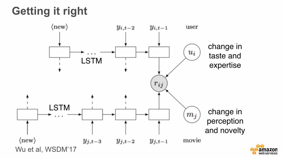
Getting it right

change intaste andexpertise

change inperceptionand novelty

LSTM

LSTM

Wu et al, WSDM’17

Wu et al, WSDM’17

Prizes

Sanity Check

Deep Learning with MXNet

Caffe Torch Theano Tensorflow CNTK Keras Paddle

(image - Banksy/wikipedia)

Why yet another deep networks tool?

Why yet another deep networks tool?• Frugality & resource efficiency

Engineered for cheap GPUs with smaller memory, slow networks • Speed

• Linear scaling with #machines and #GPUs • High efficiency on single machine, too (C++ backend)

• Simplicity Mix declarative and imperative code

single implementation of backend system and common operators

performance guarantee regardless which frontend

language is used

frontend

backend

Imperative Programs

import numpy as np a = np.ones(10) b = np.ones(10) * 2 c = b * a print c d = c + 1 Easy to tweak

with python codes

Pro • Straightforward and flexible. • Take advantage of language native

features (loop, condition, debugger)

Con • Hard to optimize

Declarative Programs

A = Variable('A') B = Variable('B') C = B * A D = C + 1 f = compile(D) d = f(A=np.ones(10), B=np.ones(10)*2)

Pro • More chances for optimization • Cross different languages

Con • Less flexible

A B

1

+

⨉

C can share memory with D, because C is deleted later

Imperative vs. Declarative for Deep LearningComputational Graph

of the Deep Architecture

forward backward

Needs heavy optimization, fits declarative programs

Needs mutation and more language native features, good for

imperative programs

Updates and Interactions with the graph

• Iteration loops • Parameter update

• Beam search • Feature extraction …

w w � ⌘@wf(w)

Mixed Style Training Loop in MXNet

executor = neuralnetwork.bind() for i in range(3): train_iter.reset() for dbatch in train_iter: args["data"][:] = dbatch.data[0] args["softmax_label"][:] = dbatch.label[0] executor.forward(is_train=True) executor.backward()

for key in update_keys: args[key] -= learning_rate * grads[key]

Imperative NDArray can be set as input nodes to the graph

Executor is bound from declarative program that

describes the network

Imperative parameter update on GPU

Mixed API for Quick Extensions

• Runtime switching between different graphs depending on input • Useful for sequence modeling and image size reshaping • Use of imperative code in Python, 10 lines of additional Python code

BucketingVariable length sentences

3D Image Construction

Deep3D

100 lines of Python code

https://github.com/piiswrong/deep3d

Distributed Deep Learning

Distributed Deep Learning

## trainnum_gpus = 4gpus = [mx.gpu(i) for i in range(num_gpus)]model = mx.model.FeedForward( ctx = gpus, symbol = softmax, num_round = 20, learning_rate = 0.01, momentum = 0.9, wd = 0.00001)model.fit(X = train, eval_data = val, batch_end_callback = mx.callback.Speedometer(batch_size=batch_size))

2 lines for multi GPU

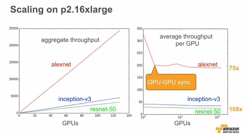
Scaling on p2.16xlarge

alexnet

inception-v3

resnet-50

GPUs GPUs

average throughput per GPUaggregate throughput

GPU-GPU sync

alexnet

inception-v3

resnet-50 108x

75x

Getting Started

• Website http://mxnet.io/

• GitHub repository git clone —recursive [email protected]:dmlc/mxnet.git

• Dockerdocker pull dmlc/mxnet

• Amazon AWS Deep Learning AMI (with other toolkits & anaconda)https://aws.amazon.com/marketplace/pp/B01M0AXXQBhttp://bit.ly/deepami

• CloudFormation Template https://github.com/dmlc/mxnet/tree/master/tools/cfn http://bit.ly/deepcfn

https://aws.amazon.com/marketplace/pp/B01M0AXXQB

Acknowledgements

• User engagementHow Jing, Chao-Yuan Wu

• Temporal recommendersChao-Yuan Wu, Alex Beutel, Amr Ahmed

• MXNet & Deep Learning AMIMu Li, Tianqi Chen, Bing Xu, Eric Xie, Joseph Spisak, Naveen Swamy, Anirudh Subramanian and many more …

We are hiring {smola, thakerb, spisakj}@amazon.com

http://amazon.com

alex smola, director of machine learning, aws/amazon, at mlconf sf 2016

Technology