alessandro manacorda · kinetics models of granular and active matter: hydrodynamics and...

Kinetics Models of Granular and Active Matter:

Hydrodynamics and Fluctuations

Alessandro Manacorda

Universita degli studi di Roma Sapienza

January 26, 2015

Alessandro Manacorda Kinetics Models of Granular and Active Matter: Hydrodynamics

Non-equilibrium Physics

A physical system is out of equilibrium when its macroscopicdynamics is not invariant under time inversion.

→ Nonequilibrium is ubiquitous!

thermodynamic transformations

chemical reactions

biological systems

weather

financial processes

your breathe in this moment

Nonequilibrium statistical mechanics:→ approach to equilibrium, NonEquilibrium Stationary States(NESS), critical phenomena, hydrodynamics, complex systems,

chaos theory ...


Non-equilibrium Physics

A physical system is out of equilibrium when its macroscopicdynamics is not invariant under time inversion.

→ Nonequilibrium is ubiquitous!

thermodynamic transformations

chemical reactions

biological systems

weather

financial processes

your breathe in this moment

Nonequilibrium statistical mechanics:→ approach to equilibrium, NonEquilibrium Stationary States(NESS), critical phenomena, hydrodynamics, complex systems,

chaos theory ... granular and active matter


Granular Matter

A granular systems is made ofgrains:

classical grains

in experiments,N ∼ 103 ≪ NA

dissipative interactions

sand, cereals, icebergs, Saturnrings...

⇓

metastable stationary states

non gaussian velocitydistributions

correlations

patterns, segregation,frustration...

phase transitions


Active Matter

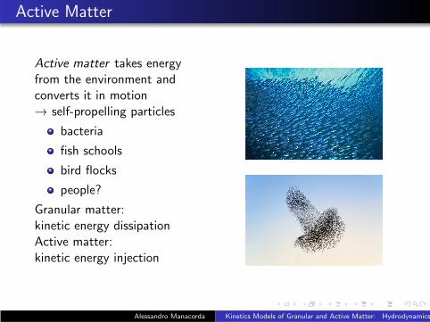
Active matter takes energyfrom the environment andconverts it in motion→ self-propelling particles

bacteria

fish schools

bird flocks

people?

Granular matter:kinetic energy dissipationActive matter:kinetic energy injection


Kinetic Theory and Hydrodynamics

Nonequilibrium → no hamiltonian H and equilibrium definitions

Microscopic dynamics

Langevin equation

Noise over initial conditions

Kinetic theory ⇒ phase-space distribution P({r , v} , t), Boltzmannequation

∂tP + v · ∇rP +F

m· ∇vP =

(

∂P

∂t

)

coll

Hydrodynamics

Coarse-graining of the system

Conservation laws → balance equations for conserved fields varying overlong time and space scales

n(r, t) =

∫d3NvP(r, v, t), u(r, t) =

∫d3Nv vP(r, v, t), T (r, t) =

∫d3Nvv2P(r, v, t)

e.g. Navier-Stokes eq.

ρ∂tu+ ρ(u · ∇)u = f −∇P + η∇2u


Fluctuating Hydrodynamics and Macroscopic Fluctuations

Theory

Fluctuating hydrodynamics

Useful representation for granular and active matter hydrodynamics

Small number of particles → fluctuations become relevant →stochastic hydrodynamic equations

Local equilibrium approximation → local gaussian white noise

Macroscopic fluctuations theory

Recently developed theory (Bertini, De Sole, Gabrielli, Jona-Lasinio,Landim; 2001-2014)

Density and current fluctuations from large deviation theory withoutlocal equilibrium approximation

Developed for non-equilibrium stationary states of driven diffusivesystems

Hard technical challenge


Lattice Models

Goal:microscopic kinetics ⇒ transport coefficients, current fluctuations,

macroscopic stochastic equations and dynamics

1980: Kipnis-Marchioro-Presutti (KMP) → lattice hydrodynamicalmodel with conserved energy

{ρi}Ni=1 , ρ′i = p(ρi + ρi+1) , ρ′

i+1 = (1− p)(ρi + ρi+1)

2010-2013: Prados, Lasanta and Hurtado → similar system withenergy dissipation ∝ (1− α)(ρi + ρi+1)

{ρi}Ni=1 , ρ′i = pα(ρi + ρi+1) , ρ′

i+1 = (1− p)α(ρi + ρi+1)

⇓

Development of MFT and Fluctuating HydrodynamicsLack of microscopic theory with conserved momentum


BBP Model

2002: Baldassarri, Bettolo and Puglisi → microscopic model withvelocities

periodic chain of L particles with transversal velocities

Maxwell molecules

momentum conservation

energy dissipation

Discrete space-time stochastic continuity equation:

vl ,p+1 = vl ,p − jl ,p + jl−1,p

jl ,p = 1+α2 δyp ,l (vl ,p − vl+1,p)

(1)


Hydrodynamic Equations

Quasi-elastic limit:

L ≫ 1, α→ 1L2(1− α2) = ν <∞

Time-length scaling:

∆x = 1/L∆t = 1/L3

Local equilibrium approximation:

P(vl , vm; p) = Pp(vl)Pp(vm)

=1

2π√

Tl ,pTm,p

exp

[

−(vl − ul ,p)2

2Tl ,p− (vm − um,p)

2

2Tm,p

]


Hydrodynamic Equations

Quasi-elastic limit:

L ≫ 1, α→ 1L2(1− α2) = ν <∞

Time-length scaling:

∆x = 1/L∆t = 1/L3

Local equilibrium approximation:

P(vl , vm; p) = Pp(vl)Pp(vm)

=1

2π√

Tl ,pTm,p

exp

[

−(vl − ul ,p)2

2Tl ,p− (vm − um,p)

2

2Tm,p

]

⇓Hydrodinamics

∂tu(x , t) = ∂2xu(x , t)

∂tT (x , t) = ∂2xT (x , t)− νT (x , t) + 2 (∂xu(x , t))2

(2)

diffusion sink viscous heating


Cooling Regimes

Homogeneity ⇒ u(x , t) = ∂x = 0⇓

Homogeneous cooling state:THCS(t) = T0e

−νt (Haff 1983)

Rescaled fields:u = u/

√THCS , T = T/THCS

→ stationary cooling state

Linear analysis:

{

∂t u(k , t) =(

ν/2− k2)

u(k , t)

∂tT (k , t) = −k2T (k , t)

⇒ homogeneous cooling stable forν < νc = 8π2

1e-05

0.0001

0.001

0.01

0.1

1

0 0.2 0.4 0.6 0.8 1

T(t

)

t

L = 1000ν = 10ν = 20ν = 30ν = 40

e-10 t

e-20 t

e-30 t

e-40 t

0.04

0.06

0.08

0.1

0.12

0.14

0.16

0.18

0 0.02 0.04 0.06 0.08 0.1 0.12u m

ax /

T1/

2 HC

S (

t)

t

A = 0.1, L = 1000ν = 68ν = 78ν = 79ν = 98

umax (t,68)umax (t,78)umax (t,79)umax (t,88)


Nonhomogeneity

No symmetry for space translations ⇒ Nonhomogeneous regimeFirst mode → exact solution

u(x , 0) = u0 sin(2πx), T (x , 0) ≡ T0

⇓{

u(x , t) = u0 sin(2πx)e−νc t/2

T (x , t) = T0e−νt +

νcu202 e−νc t

[

1−e−(ν−νc )t

ν−νc+ cos(4πx)1−e−(ν+νc )t

ν+νc

]

.

(3)

-0.4

-0.3

-0.2

-0.1

0

0.1

0.2

0.3

0.4

0 0.1 0.2 0.3 0.4 0.5 0.6 0.7 0.8 0.9 1

u(x,

t)

x

A = 1, ν = 68, L = 1000

t = 2/ν 0.24

0.25

0.26

0.27

0.28

0.29

0.3

0 0.1 0.2 0.3 0.4 0.5 0.6 0.7 0.8 0.9 1

T(x

,t)

x

A = 1, ν = 68, L = 1000

t = 2/ν


Correlations and Failure of LE

Numerical simulations ⇒ LE good approximation withdiscrepancies

Momentum conservation ⇒ non-zero correlationsC (x , t) = 〈v(0, t)v(x , t)〉Closed set of equations for correlations without LE ⇒diffusion equation with PB and symmetric profile

∂t C (x , t) = 2∂2x C (x , t)+νC (x , t)


Correlations and Failure of LE

Numerical simulations ⇒ LE good approximation withdiscrepancies

Momentum conservation ⇒ non-zero correlationsC (x , t) = 〈v(0, t)v(x , t)〉Closed set of equations for correlations without LE ⇒diffusion equation with PB and symmetric profile

∂t C (x , t) = 2∂2x C (x , t)+νC (x , t)

⇓Stationary correlation

C∞(x) ≃ −L−1 1

2

√

ν

2

cos[√

ν2

(

x − 12

)]

sin(

12

√

ν2

)

-3.5

-3

-2.5

-2

-1.5

-1

-0.5

0

0.5

1

1.5

2

0 0.1 0.2 0.3 0.4 0.5

D~ (

x,t)

x

Rescaled spatial correlation, MM

L=250, ν=40νt = 0νt = 5

νt = 10D~

th(x)


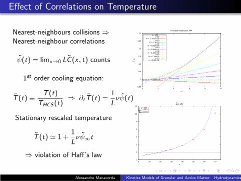
Effect of Correlations on Temperature

Nearest-neighbours collisions ⇒Nearest-neighbour correlations

ψ(t) = limx→0 LC (x , t) counts

1st order cooling equation:

T (t) ≡ T (t)

THCS(t)⇒ ∂tT (t) =

1

Lνψ(t)

Stationary rescaled temperature

T (t) ≃ 1 +1

Lνψ∞t

⇒ violation of Haff’s law

0.95

1

1.05

1.1

1.15

1.2

1.25

1.3

0 2 4 6 8 10

T~ (

t)

ν t

Rescaled temperature, MM

L = 250ν=10

m = -2.1912e-03ν=20

m = -1.9e-05ν=30

m = 2.825e-03ν=40

m = 6.964e-03ν=50

m = 1.316e-02ν=60

m = 2.38e-02ν=70

m = 4.08e-02

-2

0

2

4

6

8

10

12

0 10 20 30 40 50 60 70

ν

ψ~

(ν), MM

L = 250ψ~

expψ~

th


Further Analysis

Maxwell molecules vs hard spheres?

Energy fluctuations σ2E (t) =

〈E 2(t)〉−〈E(t)〉2

〈E(t)〉2 ⇒ Multiscaling?

Nonhomogeneous profile ⇒ momentum and energy currents, j(x , t)and JE (x , t) = 〈(vl,p + vl+1,p) jl,p〉Velocity distribution P({v}) and local equilibrium

Thermostat ⇒ Heat flux? Linear response? Entropy production?Fluctuation-dissipation?

-15

-10

-5

0

5

10

15

0 0.1 0.2 0.3 0.4 0.5

D~(x

)

x

Rescaled correlation profiles

L=250, νt=9ν=40, MMν=40, HSν=70, MMν=70, HS

0.95

1

1.05

1.1

1.15

1.2

1.25

1.3

0 2 4 6 8 10

T~(t

)

ν t

Rescaled temperature

L = 250ν=10, MMν=10, HSν=40, MMν=40, HSν=70, MMν=70, HS


Perspectives

Molecular vs lattice models

Active matter have inertia ⇒ theoretical models ofself-propelled particles with inertia

General laws for fluctuations, transport coefficients, FDTbeyond phenomenological approach

Comparison with experiments and patterns for furtherinvestigations


alessandro manacorda · kinetics models of granular and active matter: hydrodynamics and...

Documents