AladinUser manual

Pierre Fernique

1 IntroductionAladin is an interactive software sky atlas allowing the user to visualize digitized astronomical images, superimpose entries from astronomical catalogues or databases. Most of available image and catalogue over the Internet are available and notably SIMBAD, NED, VizieR, MAST/STScI, CADC, HEASARC, SLOAN, NVSS… Aladin is dedicated to professional astronomers. It can be also used by teachers or undergraduate students or amateur astronomers. It is free under ULP/CNRS licence (see the copyright). It has been translated in English, French, Italian, Russian, Chinese…

1

Aladin is mainly used for : Visualizing and checking catalogues and images Searching and browsing available astronomical data Preparing observations Creating field charts

The Aladin software can be used directly in a Web page for dynamically visualizing astronomical data into a simple navigator such as Internet Explorer or Firefox. Many institutes are using this way for providing their own data to their users (NED, CADC, MAST, ESAC, ESO..).

Aladin is developped by the Centre de Données astronomiques de Strasbourg (CDS). It is compatible with most computer configurations including Windows, Linux and Mac. It does not require significant resources unless it has to handle very large images (several gigabytes) or very large catalogues (several hundreds of thousands of objects)

Created in 1999, Aladin is supporting emerging standards of the Virtual Observatory. It is compliant with other visualization and analysis tools (IDL, VOPlot, TOPCAT, Specview, Splat, VOSpec ...). All these key topics allow Aladin to be a powerful data exploration and integration tool as well as a science enabler.

The Aladin Web site is : http://aladin.u-strasbg.fr.

2 Installation

The Aladin installation depends on your hardware configuration. In any case, it only takes a few seconds.

Local installation

Aladin requires only a few megabytes disk space and 256 RAM megabytes is sufficient for most jobs.

Under WindowsURL : http://aladin.u-strasbg.fr/java/Aladin.exe

Under Windows, the fastest and easiest way consist to copy the file “Aladin.exe” in a folder, or even directly on your desktop. That's all!

Under Mac URL: http://aladin.u-strasbg.fr/java/Aladin.dmg

Installation under Macintosh uses a classic “dmg” package. Download it, open it, and copy the “Aladin.app” file in your “Applications” folder. That’s all!

2

Under Linux and other Unix systems URL: http://aladin.u-strasbg.fr/java/Aladin.jar

Installation under Linux is both simpler and more complicated. More complicated because there is no single standard installation, easier because everything is clear, nothing is hidden. We suggest you to copy the “Aladin.jar” file in a folder. And then launch Aladin in a console "by hand" with this following command line: java –jar Aladin.jar

Tip: You can write a small file containing the parameters required for your jobs. For instance, if you want to launch Aladin with 1 gigabytes RAM you can create a file called “Aladin” containing this single line:

java –Xmx1024m –jar Aladin.jar $*

Note: Aladin can be used with local data. However it is better to have an Internet connection (≥ 512Kbit/s) for also accessing astronomical databases. For details about Aladin installation or for downloading the latest beta version, see this Web page:

http://aladin.u-strasbg.fr/java/nph-aladin.pl?frame=downloading

Aladin in applet

Aladin can be used without any installation, directly in your Web browser. By using one of these following URLs, your browser will automatically load the Aladin code and then will execute it in its own window. Aladin has been designed for starting as fast as possible (less than 2 megabytes).

France – Strasbourg (CDS) : http://aladin.u-strasbg.fr/java/nph-aladin.pl Canada – Victoria (CADC) : http://vizier.hia.nrc.ca/viz-bin/nph-aladin.pl United Kingdom – Cambridge: http://archive.ast.cam.ac.uk/viz-bin/nph-aladin.pl Japan – Tokyo (ADAC) : http://vizier.nao.ac.jp/viz-bin/nph-aladin.pl India – Puna (IUCAA) : http://urania.iucaa.ernet.in/viz-bin/nph-aladin.pl USA – Harvard (CFA) : http://vizier.cfa.harvard.edu/viz-bin/nph-aladin.pl

You must accept the applet execution (certification). If not, Aladin will start but in crippled mode reducing its performances and capabilities.

3

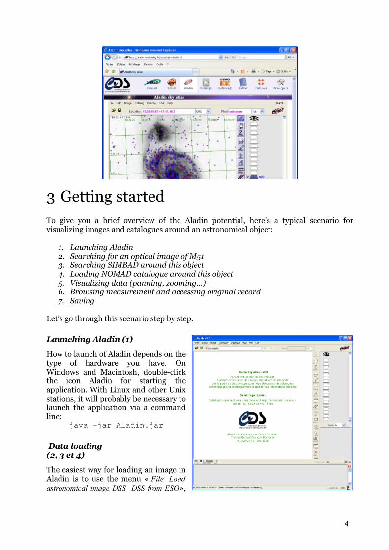
3 Getting startedTo give you a brief overview of the Aladin potential, here's a typical scenario for visualizing images and catalogues around an astronomical object:

1. Launching Aladin2. Searching for an optical image of M513. Searching SIMBAD around this object4. Loading NOMAD catalogue around this object5. Visualizing data (panning, zooming…)6. Browsing measurement and accessing original record7. Saving

Let’s go through this scenario step by step.

Launching Aladin (1)

How to launch of Aladin depends on the type of hardware you have. On Windows and Macintosh, double-click the icon Aladin for starting the application. With Linux and other Unix stations, it will probably be necessary to launch the application via a command line:

java –jar Aladin.jar

Data loading(2, 3 et 4)

The easiest way for loading an image in Aladin is to use the menu « File Load astronomical image DSS DSS from ESO»,

4

and to specify a name or an object position in the form that appears. In our example « M51 ».

And then, just press the « SUBMIT » button.

The form opened in the previous step displays the data server that Aladin can access. The image server appears on the left side. In fact, the previous step has pre-selected the corresponding form, here « DSS from ESO ». On the right side appear the tabular data servers (SIMBAD, NED…) and most of astronomical catalogues via VizieR.Thus, for loading Simbad data, you have to click on the Simbad tab,

and without changing the parameter value in the form fields (identical to the previous position), press the « SEARCH » button again. Notice that for a catalogue, you have to write its name in the VizieR form before submitting the request. In our example, as NOMAD is a large survey, you can directly select it in the « Surveys » tab by clicking on the corresponding line. After that, you must press the « SEARCH » button.

Data visualization (4)

the data visualization uses the main Aladin window. This window has 4 components:

1. The stack: shows all the downloaded data as a stack of « planes ». The user eye is on the top of this stack and sees all activated planes by transparency.

2. The zoom: shows the image area currently visible (blue rectangle) according to the factor and the centre of the zoom.

3. The view: displays the image area currently visible according to the activated stack planes and the zoom and superimposes graphic symbols corresponding to the astronomical objects in loaded catalogues and

tables.4. The measurements: shows the measurements associated to the objects

selected in the view via the mouse (magnitude, parallax…)

Plane activation: Enabling or disabling a plane is done by clicking on the small checkbox on the left of the plane logo in the stack. It is also possible to switch planes via

5

the mouse (click and drag) to change the foreground plane for a better seeing of the view (e.g. an image on top of the stack hides catalogs below).

Z oom setting: The fastest way for adjusting the zoom is to use the mouse wheel with the mouse located in the “view” or in the “zoom” frame. If your mouse does not have a wheel, you can use the “zoom selector” just above the “zoom” frame.

Moving in the image: For image moving, click and drag the blue rectangle visible in the “zoom” frame.

Centring on a particular object: The view centre displays a reticule (the magenta cross). The easiest way for pointing on a particular object is to set the reticule on this object by clicking on it, then zooming by using the mouse wheel. The view will be automatically centred on this object.

Measurements and original record access (6)

The view can display graphical objects associated to astronomical catalogs or tables in overlay of the background image - in this case SIMBAD and NOMAD. Each of these objects can be selected via a mouse selection (direct click on a object or mouse box selection).

The selected objects appear surrounded by with a small green square. The associated measurements are displayed as a table in the measurement frame. Some values are underlined in blue as a "Web link".

By clicking on a link, Aladin opens your browser and displays additional information. The first link is usually used to display the full original record.

6

Saving (7)

Aladin offers several saving options: for keeping the current view as an image, for getting an EPS file for scientific publication, etc. Use the menu « File Save the current view PNG » for getting an image file of the current view in a format that you will easily use in any desktop tools.

After this brief Aladin introduction, let’s go deeper to the available process.

4 Available Aladin processing overviewAladin works mainly on 3 types of data: images, catalogs and graphic overlays. These data types are displayed in one or several "views". For each of these elements, Aladin has a set of tools.

7

Aladin definitions

An astronomical image is a rectangular array of values representing a field of view of the sky. The astronomical image is usually provided with other information about its origin and its calibration (sky position, pixel size, type of projection...);

An astronomical catalog is a table, or several tables, for which each row contains information about an astronomical object called a "source" (ID, sky position, physical measurements...);

A graphical overlay is one or several graphical shapes (line, circle, polygon…) associated to sky positions;

A view is a projection of a image area on which has drawn catalog source symbols and/or graphical overlays;

The sky position is considered as a couple of angles (RA - right ascension, DEC - declination) specifying a celestial sphere position. Aladin does not manipulate the concept of distance to the observer.

We will briefly describe the available Aladin operations on images, catalogs, graphical overlays and views.

8

Image processing functions

Pixel range adjustments (contrast); Symmetry (top bottom, right left); Image colour composition from 3 original images; Image mosaicing; Cube generation from several images covering the same field; Image resampling (image re-projection according to the astrometrical solution of

another image); Image astrometrical calibration (by parameters or by matching stars); Pixel computations (addition, subtraction, multiplication, division, convolutions,

normalisation).

Note: In case of « huge images » (several gigabytes), only the basic processing functions are available (pixel adjustment, symmetry)

Catalogue processing functions

9

Source measurement operations (selection, filtering, sorting, tagging….); Graphical symbol drawing according to some source measurement values (e.g. circles

proportional to the magnitude, arrows based on the proper movements, error ellipses...);

Catalog cross correlation; Catalog column generator; Catalog astrometrical calibration (without sky coordinates).

Graphical overlays processing functions

Contour extraction; Graphical tools:

Distance measurement; Tag tool; Hand drawn tool; Free text; Cut graph along a segment or in the 3rd

dimension for cubes. Coordinate grid; Instrument field of view (FoV) overlays;

moving; rotation.

View operations

Catalogue sources, graphical shapes, images drawn on a background image (with transparency control support);

Zooming and panning; Display of several views simultaneously (2,4,9

or 16 views); View synchronization (same scale, same

orientation); Thumbnail view generator for a list of objects; Full screen display.

These functions can be operated via a standard graphical interface. As usual in this type of software, several alternatives are available for satisfying various work habits:

1. The menu bar on the top of the window;2. The tool bar (list of clickable buttons);

3. Popup menus available via a mouse right click or CTRL click (Mac);4. Some keyboard shortcuts.

1

Note: it is also possible to perform these operations via a script mode via described at the end of this manual (cf. )

We will discover the various GUI components and how they work.

5 The graphical interface in detailsAladin offers a rich graphical interface for achieving in a few clicks most basic functions. The two main windows are: The « main window» for displaying and manipulating the data; The « server selector» for locating and accessing the astronomical data, locally or via

Internet.

Several other windows allow various controls, including: The pixel range control (contrast); The contour generator; The catalog filter editor; The catalog cross correlation; The catalog column computing; The astrometrical calibration controller; The image resampling controller; The arithmetic operations on image pixel values; The saving controller; The user preferences (configuration); The console for using the script mode.

We will now review the various interface elements, their role,

Note: It is possible to start Aladin in « students » mode (« undergraduate ») or in simple display mode (« preview ’) in order to adapt the Aladin interface to the user profile. These two modes will be studied later.

5.1 The main windowAladin combines in a single window most of the components required for displaying and manipulating data: a menu bar, a location box, the view panel, the zoom panel, the stack, and a panel for the measurements.

1

Tip: The relative proportions of the different components can be adjusted using the double crossed arrow icon on the bottom of the tool bar. Click and Drag for adjusting the component proportions.

Guided tour

Menu: Help Aladin guided tour…Help Show me how to…

For discovering the main window, Aladin offers a "guided tour" you will find in the « Help » menu. Once activated, use your mouse over the various elements of the main window for displaying a description of the pointed component.

In addition, Aladin offers a series of « demonstrations » available via the « Help Show me how to… » Menu. During a demonstration, a dialog window describes step by step the operations and simultaneously, the mouse pointer will move alone displaying the corresponding actions.

1

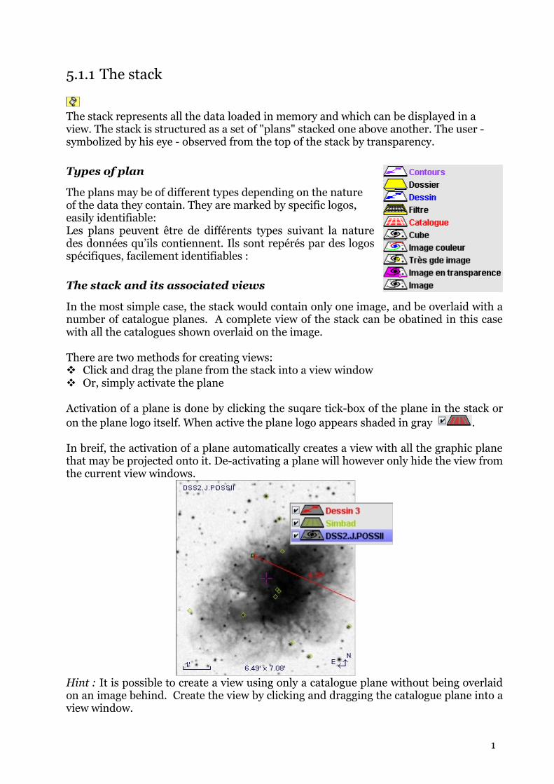
5.1.1 The stack

The stack represents all the data loaded in memory and which can be displayed in a view. The stack is structured as a set of "plans" stacked one above another. The user - symbolized by his eye - observed from the top of the stack by transparency.

Types of plan

The plans may be of different types depending on the nature of the data they contain. They are marked by specific logos, easily identifiable:Les plans peuvent être de différents types suivant la nature des données qu’ils contiennent. Ils sont repérés par des logos spécifiques, facilement identifiables :

The stack and its associated views

In the most simple case, the stack would contain only one image, and be overlaid with a number of catalogue planes. A complete view of the stack can be obatined in this case with all the catalogues shown overlaid on the image.

There are two methods for creating views: Click and drag the plane from the stack into a view window Or, simply activate the plane

Activation of a plane is done by clicking the suqare tick-box of the plane in the stack or on the plane logo itself. When active the plane logo appears shaded in gray .

In breif, the activation of a plane automatically creates a view with all the graphic plane that may be projected onto it. De-activating a plane will however only hide the view from the current view windows.

Hint : It is possible to create a view using only a catalogue plane without being overlaid on an image behind. Create the view by clicking and dragging the catalogue plane into a view window.

1

Image planes of the same field may be compared in various ways. One image may be overlaid on another with a controlled level of transparency (see section ?). Alternatively a colour composite of the two (or three) image may be constructed, and multiple images may be directly compared by creating 'blink' planes.

It is possible to load the stack with images and catalogues that do not fall in the same part of the sky. Using a single view window, it is possible to switch between different fields by clicking on the relevant image planes. Also, using multiple view windows will allow simultaneous viewing of different fields.

Heirarchical structure of the stack

The stack may be organised into a multiple level structure by the use of folders. Folders may be created using the main menu item Edit-> Create a Stack Folder, and Edit->Insert in a New Stack Folder. These tasks may also be accessed by right-clicking, or CTRL-click in the stack.

Contextual Menu

The stack has a contextual menu that may be accessed by using a right-click or CTRL-click. This menu collects the tasks related specifically to stack planes, such as selecting all the objects in a plane, deleting planes, creating folders and also broadcasting planes to other applications.

Selecting Planes

Selecting a plane in a stack is done by clicking on the name of the plane (compared to activating a plane which is done by the clicking the plane logo or the tick-box). Selected planes are indicated by bright blue highlighting. Multiple planes may be selected by pressing the CTRL key while making the selections, or by using the Shift key to select consecutive planes. when planes are selected, certain items of the contectual and main menus will be active or non-active depending on the nature of those planes. For example, the contour task will be active when an image is selected, but not active for a catalogue.

1

Plane Properties

Bouton : prop. Menu : Edition PropriétésRaccourci : Ctrl + Entrée

The « prop » button brings up a window with properties of a plane. This is also available from the main menu Edit->Properties, and from the contectual menu in the stack. The propeties window lists the name of the plane and the origin of the data, and other properties dependent on the nature of the plane. Certain properties may be altered in this window. For example, the plaotting symbols and colour of catalogue planes. the window also shows the web address used by aladin to obtain the data shown.

Controlling the transparency of planes

Certain plane may be made semi-transparent so that planes beneath it in the stack may be seen. This is useful when comparing images, and also when overlaying instrument field of view planes. To control the transparency of a plane use the magenta coloured slide bar on the logo of a plane.

Hint : the level of transparency may also be controlled a larger slide bar and with percentage values from the properties window.l

Various Hints and Tips

At the top of the stack there is an 'eye' icon looking down on the stack . Clicking the eye hides all the graphics planes leaving on the image planes visible. Clicking again brings un-hides the graphics planes.

1

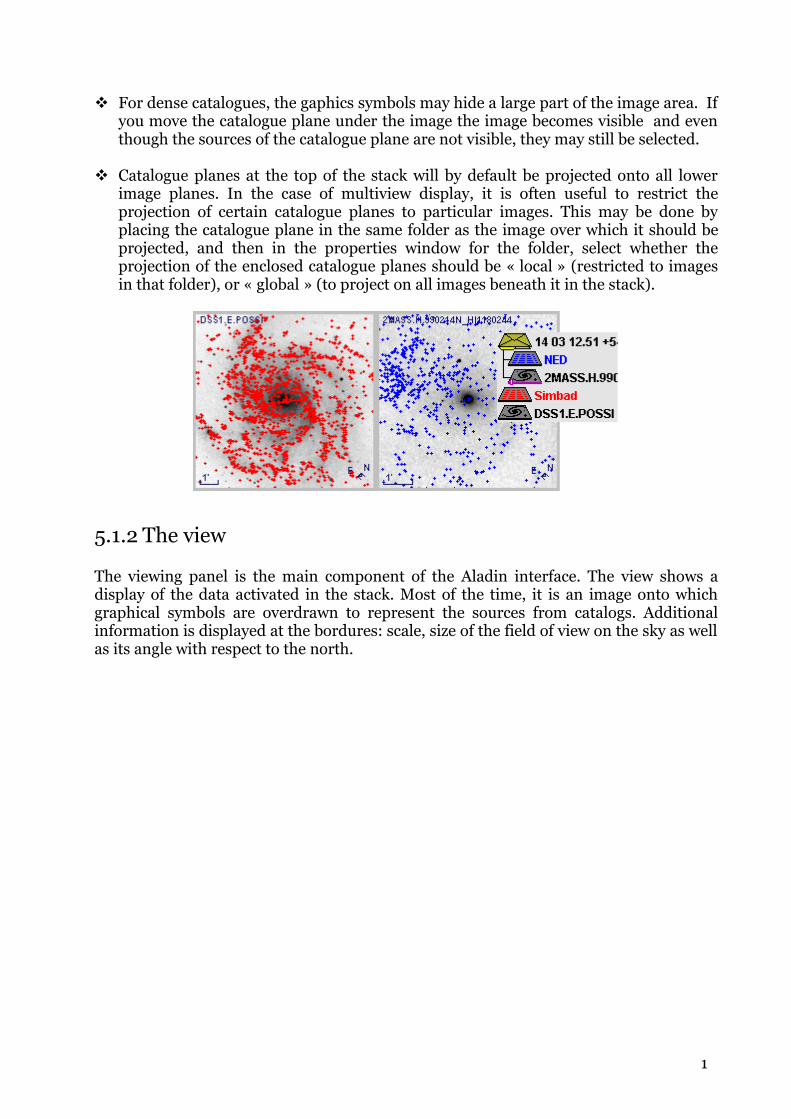
For dense catalogues, the gaphics symbols may hide a large part of the image area. If you move the catalogue plane under the image the image becomes visible and even though the sources of the catalogue plane are not visible, they may still be selected.

Catalogue planes at the top of the stack will by default be projected onto all lower image planes. In the case of multiview display, it is often useful to restrict the projection of certain catalogue planes to particular images. This may be done by placing the catalogue plane in the same folder as the image over which it should be projected, and then in the properties window for the folder, select whether the projection of the enclosed catalogue planes should be « local » (restricted to images in that folder), or « global » (to project on all images beneath it in the stack).

5.1.2 The view

The viewing panel is the main component of the Aladin interface. The view shows a display of the data activated in the stack. Most of the time, it is an image onto which graphical symbols are overdrawn to represent the sources from catalogs. Additional information is displayed at the bordures: scale, size of the field of view on the sky as well as its angle with respect to the north.

1

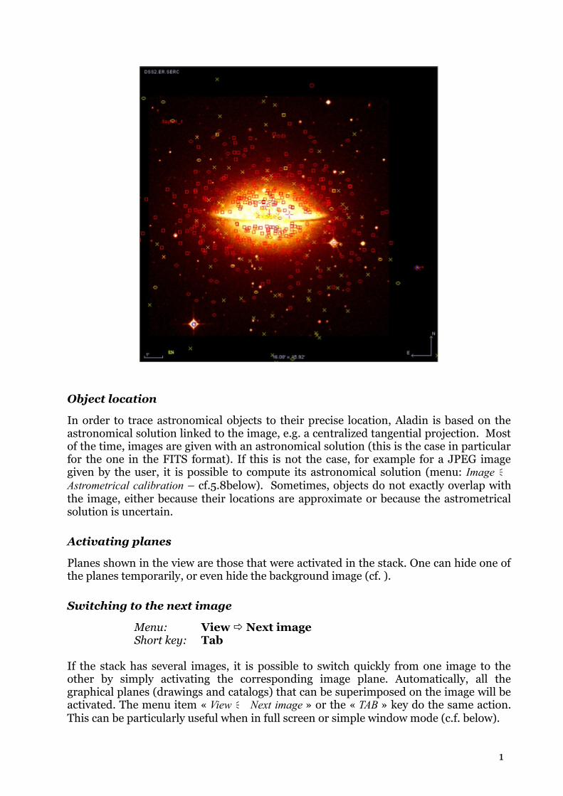
Object location

In order to trace astronomical objects to their precise location, Aladin is based on the astronomical solution linked to the image, e.g. a centralized tangential projection. Most of the time, images are given with an astronomical solution (this is the case in particular for the one in the FITS format). If this is not the case, for example for a JPEG image given by the user, it is possible to compute its astronomical solution (menu: Image Astrometrical calibration – cf.5.8below). Sometimes, objects do not exactly overlap with the image, either because their locations are approximate or because the astrometrical solution is uncertain.

Activating planes

Planes shown in the view are those that were activated in the stack. One can hide one of the planes temporarily, or even hide the background image (cf. ).

Switching to the next image

Menu: View Next imageShort key: Tab

If the stack has several images, it is possible to switch quickly from one image to the other by simply activating the corresponding image plane. Automatically, all the graphical planes (drawings and catalogs) that can be superimposed on the image will be activated. The menu item « View Next image » or the « TAB » key do the same action. This can be particularly useful when in full screen or simple window mode (c.f. below).

1

Cube or « animated sequence»

For an image data “cube” (cf. 5.10 - associations or FITS cubes), the plane in the stack holds several images that will be displayed in the view as an “animated sequence”, i.e. image after image, with a tuneable delay (400ms by default) that can be changed in the plane properties. The view, in which the cube is visualised the cube shows a pace controller overdrawn on the image. This controller uses usual conventions from tape recorder (pause, play, backward, forward,) Below the controller; a ruler displays the location of the current image in the cube. This ruler, as well as the controller can be manipulated with the mouse.

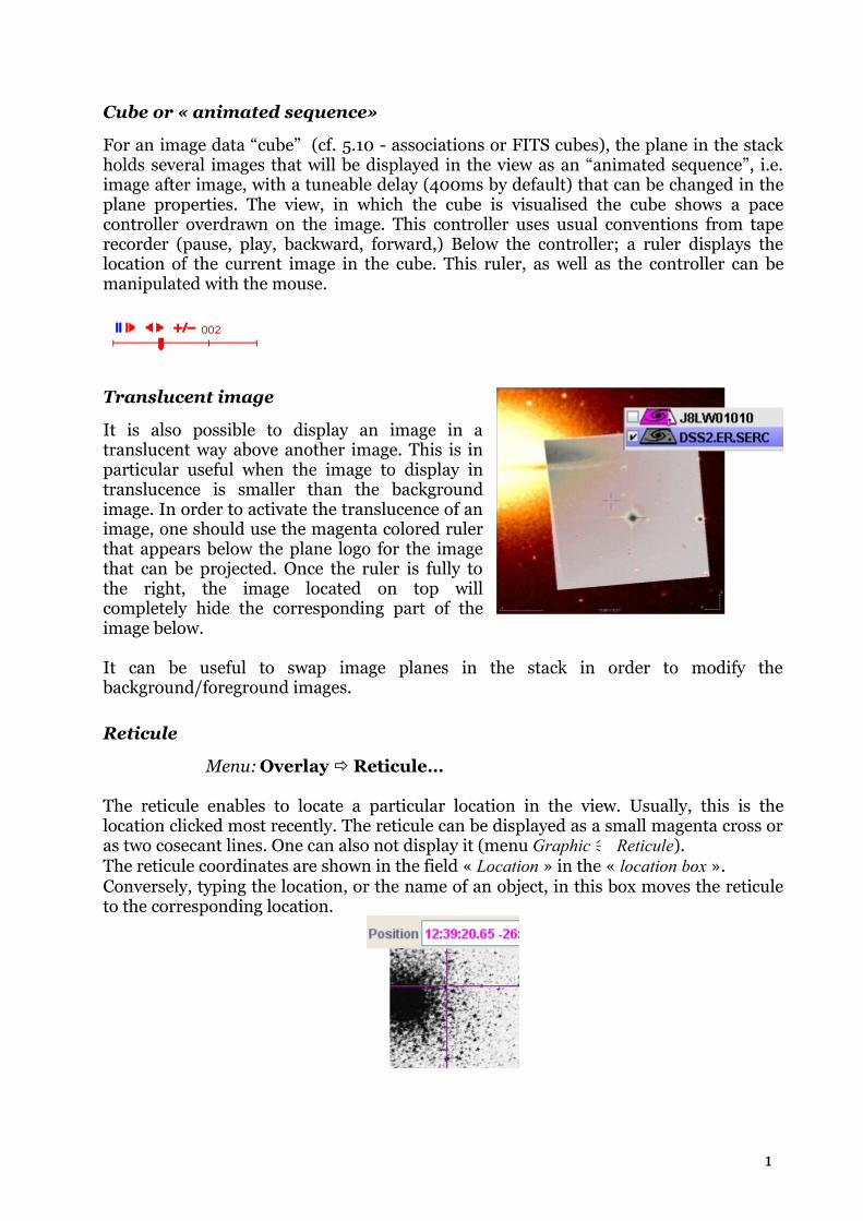
Translucent image

It is also possible to display an image in a translucent way above another image. This is in particular useful when the image to display in translucence is smaller than the background image. In order to activate the translucence of an image, one should use the magenta colored ruler that appears below the plane logo for the image that can be projected. Once the ruler is fully to the right, the image located on top will completely hide the corresponding part of the image below.

It can be useful to swap image planes in the stack in order to modify the background/foreground images.

Reticule

Menu: Overlay Reticule…

The reticule enables to locate a particular location in the view. Usually, this is the location clicked most recently. The reticule can be displayed as a small magenta cross or as two cosecant lines. One can also not display it (menu Graphic Reticule ). The reticule coordinates are shown in the field « Location » in the « location box ». Conversely, typing the location, or the name of an object, in this box moves the reticule to the corresponding location.

1

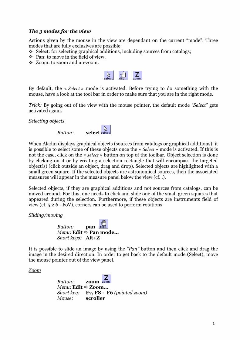
The 3 modes for the view

Actions given by the mouse in the view are dependant on the current “mode”. Three modes that are fully exclusives are possible: Select: for selecting graphical additions, including sources from catalogs; Pan: to move in the field of view; Zoom: to zoom and un-zoom.

By default, the « Select » mode is activated. Before trying to do something with the mouse, have a look at the tool bar in order to make sure that you are in the right mode.

Trick: By going out of the view with the mouse pointer, the default mode “Select” gets activated again.

Selecting objects

Button: select

When Aladin displays graphical objects (sources from catalogs or graphical additions), it is possible to select some of these objects once the « Select » mode is activated. If this is not the case, click on the « select » button on top of the toolbar. Object selection is done by clicking on it or by creating a selection rectangle that will encompass the targeted object(s) (click outside an object, drag and drop). Selected objects are highlighted with a small green square. If the selected objects are astronomical sources, then the associated measures will appear in the measure panel below the view (cf. .).

Selected objects, if they are graphical additions and not sources from catalogs, can be moved around. For this, one needs to click and slide one of the small green squares that appeared during the selection. Furthermore, if these objects are instruments field of view (cf. 5.2.6 - FoV), corners can be used to perform rotations.

Sliding/moving

Button: pan Menu: Edit Pan mode…Short keys: Alt+Z

It is possible to slide an image by using the “Pan” button and then click and drag the image in the desired direction. In order to get back to the default mode (Select), move the mouse pointer out of the view panel.

Zoom

Button: zoom Menu: Edit Zoom…Short key: F7, F8 - F6 (pointed zoom)Mouse: scroller

1

Aladin enables you to zoom in and out rapidly on a portion of an image. In order to perform rapidly, only powers of 2 factors are enabled, from 1/256 to 512 times. A factor of 2/3 was added for convenience. Below a factor ¼, a nearest neighbour algorithm is used (very “sharp” image). Between ¼ and 2/3, Aladin uses the mean, while between 2 and 512 times, pixels are duplicated (“large pixels”).

The zoom factor can be modified in many ways: By using the “zoom” button and clicking in the view (keep the Maj key pressed in

order to zoom out). In order to go back rapidly to the default mode (“select”) put the mouse pointer out of the view.

By using the mouse scroller while the mouse pointer is inside the view By using the contextual menu to the right of the window By using the main menu « Edit Zoom »

If the image has an astrometrical calibration, zooming in will centre the image on the current reticule location (unless the view was locked, c.f. below). It is therefore very simple to zoom in on a particular object, by moving the reticule onto the given object (simple click) and then using the mouse scroller.

Coordinates grid

Icon: grid Menu: Overlay GridShort key: Alt+G

Activating a grid can be done either with the “grid” icon located below the view, or using the menu « Overlay Grid ». The grid step depends on the current zoom factor in order to only display a reasonable number of sectors. The grid referential is the same as the one used to display the current location with the mouse. It is not possible to display simultaneously different grids corresponding to different referentials.

If the zoom factor is very small (1/512x), the grid can seem truncated if the astrometrical solution of the current image is inaccurate to compute a location far off the image (e.g. digitized Schmidt plate).

Target arrow

Menu: Overlay Target ArrowShort key: Alt+T

When an image was queried either by location or by object name (c.f. 5.2 – server selector), a small red arrow gives the location in the image. This arrow can be deleted using the menu item « Overlay Target Arrow ».

2

Multi-view

In order to compare more easily several images, it can be useful to create several view simultaneously. Le main panel can then be divided in 2, 4, 9 or 16 sub-panels. Each of these panels can display a different image and superposed graphical additions. These images can sample different regions of the sky or the same one. It is also possible to use different panels for a single image, for example in order to visualise different details in this image.

Number of views

Icon: multiview Menu: Edit Multiview …Short key: F1, Maj+F2, F2, F3, F4

Modifying the number of visible views can be done either with the « multiview » selector located at the bottom left of the view panel, or with the menu « Edit 1, 2, 4,9, or 16 panels ». If the views that are used are more numerous than the number of available panels, then a sliding bar appears on the left of the main window and enables you to access the other views. Up to several thousands of view can be created (cf. – thumbnails creations). Only the views that are visible make use of random access memory (RAM).

2

Allocations of the views The allocation of an image to a view is done by drag and drop of the respective plane logo onto the selected panel. It is also possible to create, as many views as there are images in the stack by using the menu « View Create one view per image ».

Trick: It is possible to drag and drop a JPEG, PNG, GIF, FITS image from your working environment (Windows desk, Linux Desktop, …) and/or from your web browser with a particular view.

Current view The current view, i.e. the one on which zoom functions will operate, is framed with a blue contour. One can click on a view in order to select it as the current view. By keeping the Maj key pressed, it is possible to select several view simultaneously, for example this can be used to select images that will be deleted. It is possible to see the current view (blue frame) in “monoview” by switching back to a single panel. The other views will not be deleted and will remain accessible either through the vertical scroller bar on the left of the window, or by switching back to a multiview mode. The current mode can also be seen in full screen (menu « View Full screen ») or in simple window mode (menu « View simple window ») – see below.

Matching the views

Icon: match Menu: Edit Match…Short key: Alt+S, Alt+Q

Within the multiview mode, it is possible to match the scale, and even the orientation, of different images sampling the same region in the sky. These functions are accessible via the menu « View Match scales » and « View Match scales and orientation » respectively. For the second case, the “match” button can also be used. Matching scales does not affect pixels, it only select automatically the closest centre and zoom factor in order to visualise the same region of the sky. This is not the case when matching both scales and orientation since it reprojects images using the location of the 4 corners of the image: images are identical but pixels have been put out of shape. Matched views are automatically selected and can be noticed by their blue frames. If the orientation was also matched, the affected images are framed in red.

2

Locked view Menu: View Lock view

When one double-clicks on a view, all the other views relative to the same region of the sky will be centred automatically on the clicked location. This is also the case if one clicks on the measures (cf. ). To prevent this change of central location and/or change of zooming factor, it is possible to lock a view so that it always keeps the same centre and the same zoom (Menu « View Locked view »). A locked view triggers the apparition of a small lock in its bottom left corner .

Sticked panelMenu: View Sticked panel

In order to prevent the scrolling of one or several views when one uses the vertical scrolling bar, it is possible to “stick” the panel so that it keeps its location. For this, use the menu « View Sticked panel ». A sticked panel triggers red triangulary corners and is not affected by the scrolling bar.

Moving and pasteIt is easy to move a view from a panel to the other by doing a simple click/drag/drop with the mouse. By keeping the Ctrl button pressed simultaneously, this function will create a duplicate of the view.

DeleteDeleting a view does not imply the deletion of the image and/or of the catalogs used for the view; the data remain accessible in the stack. However, deleting an image in the stack does suppress all the views using it. The menu « View Delete other views » enables you to suppress rapidly all views except the current one.

Full screen and simple window

Menu: View Full screen, Simple windowShort key: F11, F12

A view can be displayed by using the entirety of the screen. It can also be displayed in a simple window without the rest of the graphical interface (menu, stack, measures…) being shown. Using the F11 and F12 keys respectively will enable you to switch between these visualisation modes. The Escape key will make you go back to the normal display mode.

2

Outside the size of the display window, both modes are identical. The use of Aladin in « full screen » or « simple window » mode changes the normal usage in certain ways: Manipulation icons are shown on the right hand side. They enable you to

activate or not catalogs and graphical additions, display or not the coordinate grid, save the current view in PNG (or JPEG if the Maj key is pressed– this gives smaller size files but they are less sharp if there are graphical additions), switch to the next field (if it exists).

The icon enables you to go back to normal mode (similar to the « Esc. » key) Location information as well as pixel values are overlaid on the top right corner of

the image. The usage of the mouse merges the « Select. » mode with the « Pan » mode (cf. next

section – the tool bar). Basically, it is possible to move the field of view by clicking/dragging the image. It is also possible to select an object by directly clicking on it.

One can only select one source at a time. Its information measures will then be displayed as an overlay.

A script command can be typed directly in the view. It will be displayed in a frame overlaid.

If the stack is empty, a simplified form appears to let you type the name of an object or an astronomical location.

Trick: The mode « simple window » presents all the basic function from Aladin. It can be used by default ((cf. – user profiles) and in particular if Aladin is used as an applet (cf. – Aladin in a web browser)

5.1.3 The tool bar

Located vertically in between the stack and the view, the « tool bar » enables a quick access to the most used tools:

2

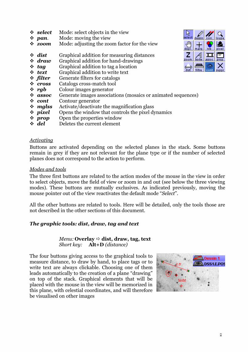
select Mode: select objects in the view pan. Mode: moving the view zoom Mode: adjusting the zoom factor for the view

dist Graphical addition for measuring distances draw Graphical addition for hand-drawings tag Graphical addition to tag a location text Graphical addition to write text filter Generate filters for catalogs cross Catalogs cross-match tool rgb Colour images generator assoc Generate images associations (mosaics or animated sequences) cont Contour generator mglss Activate/deactivate the magnification glass pixel Opens the window that controls the pixel dynamics prop Open the properties window del Deletes the current element

ActivatingButtons are activated depending on the selected planes in the stack. Some buttons remain in grey if they are not relevant for the plane type or if the number of selected planes does not correspond to the action to perform.

Modes and toolsThe three first buttons are related to the action modes of the mouse in the view in order to select objects, move the field of view or zoom in and out (see below the three viewing modes). These buttons are mutually exclusives. As indicated previously, moving the mouse pointer out of the view reactivates the default mode “Select”.

All the other buttons are related to tools. Here will be detailed, only the tools those are not described in the other sections of this document.

The graphic tools: dist, draw, tag and text

Menu: Overlay dist, draw, tag, textShort key: Alt+D (distance)

The four buttons giving access to the graphical tools to measure distance, to draw by hand, to place tags or to write text are always clickable. Choosing one of them leads automatically to the creation of a plane “drawing” on top of the stack. Graphical elements that will be placed with the mouse in the view will be memorized in this plane, with celestial coordinates, and will therefore be visualised on other images

2

Selection and MoveGraphical additions created by one of these 4 tools can be selected (Select tool) and even moved through a click/drag with the mouse. When they are selected, small green handles appear around their limits.

Technical detail: When one or several elements are moved at the same time, one should note that the displacement is computed on the celestial coordinates (RA, DEC) only for the object that is underneath the mouse pointer, and it is only then propagated to the other selected objects. Keeping the Maj key pressed will change this behaviour and only movements in XY coordinates will be considered for all objects. Both techniques do not give the same result, in particular when the objects to move are distant by more than several degrees or close to the poles.

Some tricks During a tag (« tag » tool), keeping the « Maj » pressed leads to the computation of a

centroid for the pixel values the closest to the clicked location and moves the tag to the location found. This enables you to easily put a tag at the centre of a star;

It is possible to have the location appear close to a tag. For this, select the tag of interest and use the contextual menu (right click or CTRL click) and select « label the selected objects ».

For a drawing done by hand (« draw » tool), it is possible either to keep the mouse button pressed in order to draw “continuously” or to click several times in order to draw straight lines one after the other. In this last case, it is necessary to put the mouse pointer out of the view in order to stop the drawing process, or to double-click on the last point.

In order to create a new plane, so that the graphical additions will not be in the same graphical plane, it is mandatory to press the « Maj » key while activating the tool.

Image cut associated to the distance tool When the double arrow, used to measure a distance, has been selected in the view, the zoom panel (bottom right of the main window) is replaced by an “image cut” showing the pixel values along the line measuring the distance. If this line is moved around in the view, the plot evolves as a function of the location in the image. Furthermore, if you move your mouse over the plot, a red horizontal line appears and gives the angular distance and the number of pixels for the peak below. This method is useful for example to make a quick approximation for the width at half maximum of a star.

On top of this, for an image in real colours (cf. 8.2 – supported data types), the levels for the three components Red/Green/Blue will be shown simultaneously.

2

Depth cut associated with the « Tag » tool The location and selection of a tag (with the « Tag» tool) in an image cube will generate also a cutting plot. However, this time it is along the depth of the cube. In the plot thereby obtained, the vertical red line corresponds to the location of the current image in the cube (in Aladin, a cube is seen as a sequence of images). The value mentioned at the bottom of this mark gives the physical scale corresponding to the current image in the cube (e.g. the speed). As for the distance tool, moving the tag with the mouse leads to the automatic scaling of the plot. Furthermore, going over the plot with the mouse pointer gives the value of the corresponding pixel (coordinates in the plot). A horizontal click and drag will move the red line out of the current image and hence will change the image in the current view.

The « magnifying glass » tool

Button: mglssMenu: Image Magnifier glassShort key: Ctrl+G

When the magnifying glass is activated, the zoom panel (bottom right of the main window) will be temporarily used to show a zoom of the pixels around the mouse pointer while it moves around the view.Using displacement keys (left, down, right, up arrows) is then possible to move pixel by pixel the mouse pointer.

The « del » tool

Button: DelMenu: Edit Delete

Edit Delete all

2

Short key: Del or Maj+Del

The delete tool is highly dependant on the context. Depending on the element(s) selected with the mouse, it will delete one of the following: The graphical addition(s); The view(s); The plane(s).

Furthermore, by pressing simultaneously the « Maj » key, all the data loaded in Aladin will be deleted. Use with care, there is no « undo » function in Aladin!

The other tools accessible via the tool bar are detailed in the other sections of the document.

5.1.4 The zoom panel

The « zoom panel » is located on the bottom right of the main window. It displays an illustration of the total image on which is superimposed a translucent blue rectangle.

This rectangle traces the part of the image that is shown in the view with respect to the global image. It enables the user to find his way around the global image.

The rectangle can be moved around with the mouse. The view changes automatically to show the corresponding image portion. If the visible region is completely out of the image, a red arrow will show the corresponding direction.

The overlaid information gives the angular size of the global image.

The current zoom factor can be modified easily by scrolling the mouse. In order to centre the view at the maximum size, one can click the zoom panel while keeping the Ctrl key pressed.

5.1.5 Locating band

On top of the main window, below the menu, two fields display the current location and the pixel value corresponding to the mouse pointer in the view. Each of these informations can be displayed in a specific reference system given in the folding menu located on the right of each of these fields.

Location

The location can be given in celestial coordinates or in abscissa/ordinate in the image. The celestial referentials available are ICRS, J2000, B1950, Ecliptic, Galactic,

2

Supergalactic. The display may be either sexagesimal or decimal. The accuracy of the location depends on the current zoom factor.

Pixel value

The pixel value can be given in three ways: 8 bits: The “one colour” level (usually grey) is used for current display. It gives a value

between 0 and 255 that depends mainly on the contrast parameters that were chosen. If the image is in JPEG, only this display mode will be available;

Raw file: The value used for coding pixels in the image file; Full: The « physical » value for the pixel. This value is given from the code value

(raw) multiplied by a scaling factor supplied with the image (BSCALE – according to the FITS format) and is offset from the origin (BZERO). This last value (Full) is the most significant and is the one given by default (Full=raw*BSCALE+BZERO). If the BSCALE and BZERO parameters and not given, the “Full” value for a given pixel will be the same as its “Raw” value.

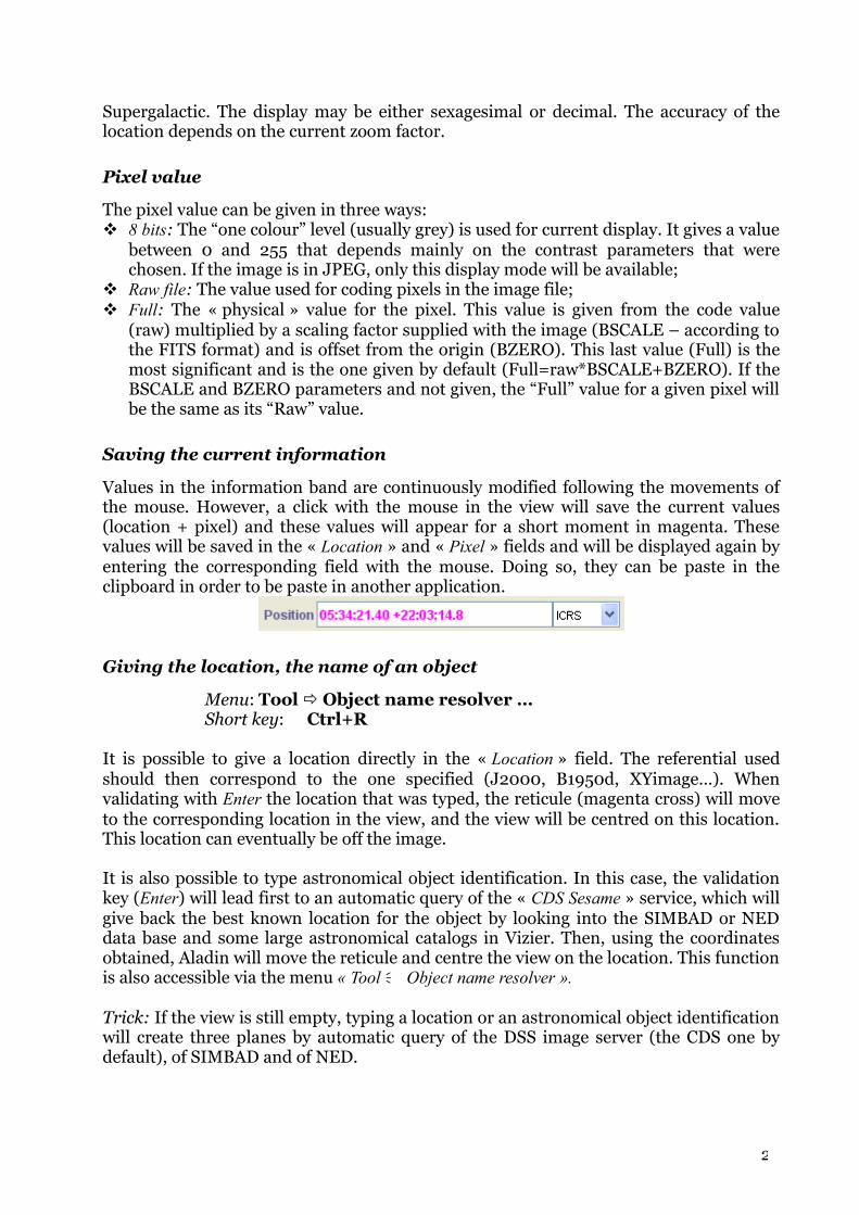
Saving the current information

Values in the information band are continuously modified following the movements of the mouse. However, a click with the mouse in the view will save the current values (location + pixel) and these values will appear for a short moment in magenta. These values will be saved in the « Location » and « Pixel » fields and will be displayed again by entering the corresponding field with the mouse. Doing so, they can be paste in the clipboard in order to be paste in another application.

Giving the location, the name of an object

Menu: Tool Object name resolver …Short key: Ctrl+R

It is possible to give a location directly in the « Location » field. The referential used should then correspond to the one specified (J2000, B1950d, XYimage…). When validating with Enter the location that was typed, the reticule (magenta cross) will move to the corresponding location in the view, and the view will be centred on this location. This location can eventually be off the image.

It is also possible to type astronomical object identification. In this case, the validation key (Enter) will lead first to an automatic query of the « CDS Sesame » service, which will give back the best known location for the object by looking into the SIMBAD or NED data base and some large astronomical catalogs in Vizier. Then, using the coordinates obtained, Aladin will move the reticule and centre the view on the location. This function is also accessible via the menu « Tool Object name resolver ».

Trick: If the view is still empty, typing a location or an astronomical object identification will create three planes by automatic query of the DSS image server (the CDS one by default), of SIMBAD and of NED.

2

Script command The location field can also be used, not only for a location, but also to type any other script command (cf. – Aladin with script)

Let’s look at the bottom of the main window: the « measures panel ».

5.1.6 The measures

The « measure panel » is located at the bottom of the Aladin main window. It is used to visualise measures associated to the sources. It is a really powerful tool that enables you to select, sort and filter tables.

Only selected sources (the selection is obtained individually or collectively in the view with the mouse - cf. ) appear in the measure panel. These measures are displayed as a table in which each line corresponds to the values associated to a source.

Selected sources are framed with a green square in the view. Moving the mouse on the selected source makes it blink and show simultaneously corresponding measures by highlighting the line in blue. Vice versa, going onto a line in the measures table makes the corresponding source blink if it is visible. Furthermore, selecting a line in the table (by clicking on it) will move the view so that it becomes centred on the corresponding source.

The first line in the table gives the header describing each column’s content. Clicking on a box in the headline leads to a sort of the lines by increasing and then decreasing order according to the column’s value. A small triangle appears on the right of the column’s name in order to indicate the sorted column. Sorting will be either alphabetical or numerical given the column’s content. It is possible to resize the width of a column by a click and drag of the right border of a box in the headline. If a box is too small to display the total value, by moving with the mouse over this box, you will temporarily see the box enlarged to unveil the remaining part of the value.

3

Measures from different catalogs

If the selected sources come from different catalogs, tables with different columns will be shown one after the other. The colour of the square at the beginning of the line is useful to disentangle them (the colour is the same as the plane in the stack).

The headline always corresponds to the last selected line (clicked with the mouse) or the one below the mouse pointer. The colour of the line below the headline is also the same as the colour of the corresponding catalog.

Links and buttons

As in a web browser, the blue underlined values are links to additional information available on the web. The web address that will be used is displayed on the bottom of the Aladin window when the mouse pointer moves over the link. By clicking with the mouse on a link, a web browser is opened and loads the corresponding web page. In general, the first link in a measure line will load the original record in the website that was gave the catalog (SIMBAD, NED, Vizier….)

Some values can also be displayed as a button. Like a web link, activating such a button leads to the loading of additional data via the internet. However, instead of leading your web browser, the loaded data will be added to the stack in order to be visualised immediately in Aladin. Most often, such data are archive images associated to an observation list.

Independent window

The measures panel can be detached from the main window by clicking on the logo at the top right . This is useful both to get a larger working space, but also to work more easily on a larger number of measures. Please note that the measure tables in Aladin can easily load several hundred thousands lines. Re-integrating the measure window to its initial location is simply done by clicking again on this same logo or by closing the window.

Sources selection

Selecting sources can be done either with the menus, with the mouse, or with a query expression.

Selection with menusMenu: Edit Select …Short key: Ctrl+A (all objects)

3

The « Edit » menu has a sub-menu that enables you to select all sources, i.e. all the sources existing in the catalogs planes loaded in the stack. It is also possible to select only the sources from one or the other plane through the menu « Edit select all objects in the selected planes ». On would have to select beforehand the aforementioned planes in the stack (cf. ).

Selection with the mouseThe selection with the mouse is the mostly used method. It enables you to choose sources given their locations in the view. In order to select a source one has to click on it in the view; To select several sources it is mandatory to include them with a selection rectangle.

To do so, one has to click on a no-source region slightly above on the left of the first source to select, and then by holding the mouse button, expand the selection by moving the mouse pointer to the bottom right. During this operation, a rectangle shows in the view the selected zone. Once you release the mouse button, all sources inside the rectangle will b selected;

To add sources to a first selection, do as described above but keep Maj Key hold.

Selection with a research expression Menu: Edit Search in loaded catalogs …Short key: Ctrl+F

Aladin gives you a very effective tool to select sources given the values of their measures. To do so, on needs to give a research expression in the « Search » box located above on the right from the measure panel.

Validating the research expression with the « Enter » key or by clicking on the small « Go » button leads to the selection of all sources which measures correspond to the research expression. Only sources from activated catalog planes will be affected (cf. – activating a plane in the stack). If the research expression is preceded by the ‘+’ sign, sources to select will be added to the current selection. Alternatively, putting the ‘-‘ sign in front of the research expression leads to deselecting the concerned sources in the sources previously selected, i.e. they will disappear from the measures table.

The search expression follows a simple and efficient syntax.This can be: A text chain; Include eventually joker keys: ‘?’ (Any key), ‘*’ (any combination of keys); Eventually it can be preceded by a column name and a test operator (=, !=, <, >, <=,

>=) to restrict the search to a particular column;Furthermore: The column name can include jokers keys (‘ ?’ or ‘*’); The column name can be surrounded by two vertical bars ‘|’ to indicate the absolute

value; There is no case distinction (capital keys or not), both for the column name and for

its value.

Comment: for convenience sake, searching with a simple text chain without any particular column indications is always considered as a sub-chain search. For example, the « gal » research will in fact be « *gal* ».

3

Some examples: Star sources which measures contain the “star” word otype=uv sources which column “otype” has the value “uv” mag*>=12 first column in which the name starts with “mag”, the numerical

value should be larger or equal to 12 |pm*|<5 same as above byt only the absolute value is taken into account type!=g* column « type » in which values that do not start with the ‘g’ letter bmag!="" column « bmag » that is not empty

UnselectingMenu: Edit Unselect objects …Short key: Ctrl+U

To unselect a source from a previous selection, click on the corresponding source while holding the Maj key.

To unselect all sources, i.e. empty the measures table, one has to click in the view anywhere outside a source or use the menu « Edit unselect all sources ».

Trick: In order to avoid loosing accidentally a selection, you can click the sources in the table so that you can re-select them afterwards (cf. section below).

CountersThe number of selected sources (i.e. the one for which sources are displayed) divided by the total number of sources is given with the counter on the bottom right of the Aladin window.

Browse through the measures

Exploring measures and most noticeably viewing rapidly the associated sources is done thanks to the selection of the specific line in the table of measures. The selected line appears with a blue background “glued to the line”, even if the mouse is not over it.

Selecting a line of measure is done either manually or with the research expression.

Select a line of measure with the mouseSelection with the mouse is done either in the measure panel with a simple mouse click (outside a web link or a button), or by clicking on a selected source in the view (green squares). It leads to a move of the reticule (magenta cross) on the corresponding sources. When the selection was done through the table, the view is automatically centred on the source (unless the view was locked - cf. ). A double-click will zoom in. Despite the difficulty to explain it in writing, it is easy to do.

3

Reminder: to redisplay the view globally, use Ctrl+ click in the zoom panel.

Selecting a line of measure with an expression The input box used to select sources is also used to select a specific line of measures. Thus, writing an expression - WITHOUT validating it (neither Enter, not the « Go » button) – and using the two arrows on each side of the input box enables you to select the previous/following measure line that corresponds to the expression. The « up arrow » and «down arrow » keys, or the mouse scroller also let you switch to the previous or the next measure respectively. If the expression is empty, then the previous/following line will simply be selected.

DeselectDeselecting the line is done with a simple mouse click in the measure panel (outside a web link or a button).

Prevented behavioursIf a line of measure is selected, some behaviours are be automatically prevented: The headline of the measure panel remains the one associated to the selected line,

even if the mouse moves outside the corresponding line (this enables you in particular to perform a sort on this table);

Moving over the other sources in the view with the mouse will not scroll through the associated measures anymore.

Checking the measures

Menu: Edit Select …, Unselect…Contextual menu: Select…, Unselect…, Keep…

A small colored square appears on the left of the line of measures. The colour code is linked to the data origins. With this square, the lines can also be checked and thus the corresponding sources, so that they can be easily found later on.

Two menus let you manipulate the checked sources: The contextual menu appears directly in the panel of measures (right click or CTRL

click):

The main menu « Edit ’:

3

In the view, sources for which the lies of measures are checked appear with a magenta square instead of the usual green one.

Add/compute a new column

Aladin gives you the possibility to add a new column of values. This operation is described with further details in section 5.7.

Export measures

Menu: Catalog Create a new plane with …Contextual menu: Create a new plane with …

Measures can be easily paste in the clipboard from the exploitation system in order to paste them to another application. The contextual menu gives several possibilities:

It is also possible to generate, through the contextual menu, a new catalog plane that will hold a copy of the sources/measures seen in the measure panel « Create a new plane with the selected sources » or in the main menu « Menu Create a new plane with the selected sources ».

Now that we have reviewed the different components from the main window, let’s go to the second mostly used window in Aladin: the « server selector ».

5.2The server selector Icon: .Menu: File Open…, File Load …Short key: Ctrl+O

The « server selector » window lets you know and query the different astronomical databases that can be accessed with Aladin.

It can be opened either with the button on the top left, or by one of the data loading menus (menu “File”…)

This window is seen as several query forms that can be selected with tabs. Tabs on the left of the window are related to images servers, tabs on the right to tables data servers, including astronomical catalogs and observations lists from telescopes (« logs »). Finally, tabs on the top are linked to special forms that will be detailed at the end of this section.

3

Tabs and forms can evolve with time and with new possibilities coming in the astronomical community. Each time it starts, Aladin accesses a “yellow pages” mechanism for the astronomical services in order to be up to date. It then adds or modifies the respective tabs when changes are detected (cf. technical details on the « cache » 8.4.2).

5.2.1 Servers list

You will find there most of the world wide astronomical centres that distribute data on the internet. Please note that some data are distributed by several institutes and it is possible to access them via different servers (e.g. the DSS is distributed by 3 servers). The servers list is described in details in the Aladin FAQ at the following address: http://aladin.u-strasbg.fr/java/FAQ.html#data

5.2.2Specifying information

Most of forms need at least two mandatory informations in order to query the sky by cone search: a target and a radius:

3

Giving the target

The target can be either the identifier of an astronomical object recognized by the Sesame process (query in SIMBAD + NED + some large catalogs), either astronomical coordinates in sexagesimal format in the J2000 referential.

Some examples:M1NGC2045Galactic centre2 31 59 +89 15 5412:59:48.70 +27:58:50.0

Giving a radius

The query radius corresponds to the radius of the cone search on the sky. This value can be followed by a unit (« ° », « ' » « "» or « deg », « arcmin », « arcsec »). The default unit is the arc minute. It is also possible to indicate a rectangular zone by using the following syntax: W x H where W is the width of the rectangle in right ascension and H is the height of the rectangle in declination. Both values can be followed by a unit. In the case where the queried server only receive cone search (on the contrary to a rectangle), Aladin will always choose a region large enough to cover the designated field (enclosing circle, on the contrary to a enclosing rectangle).

Some examples149.14’20arcmin10’ x 12’1°

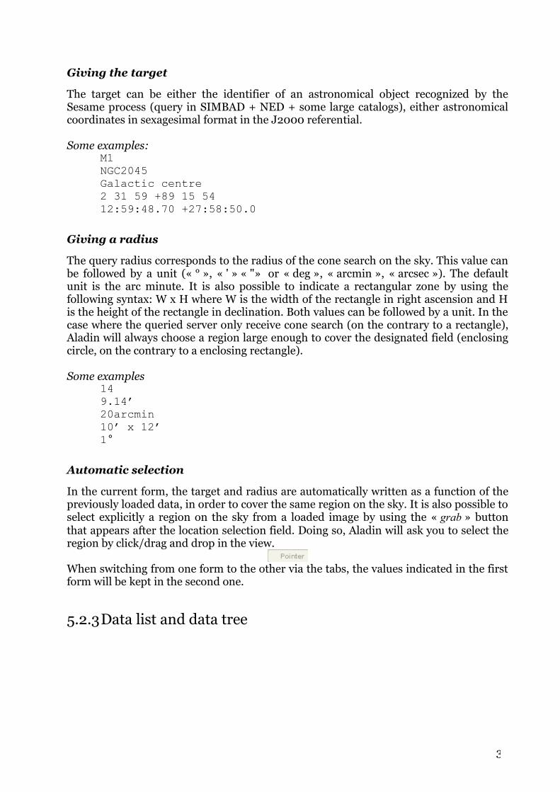
Automatic selection

In the current form, the target and radius are automatically written as a function of the previously loaded data, in order to cover the same region on the sky. It is also possible to select explicitly a region on the sky from a loaded image by using the « grab » button that appears after the location selection field. Doing so, Aladin will ask you to select the region by click/drag and drop in the view.

When switching from one form to the other via the tabs, the values indicated in the first form will be kept in the second one.

5.2.3Data list and data tree

3

Some servers need two steps to load the data: first you need to indicate the region on the sky, then you select among the available images or catalogs, those of which you would like to load. During the second step, Aladin displays the available data as a list or a table. This list/table has several functionalities : By moving the mouse on an element,

the corresponding field of view will be displayed in the main window;

If the data are shown as a data tree, a right click shows a tree control sub-menu; If the data are in list format, it is possible to sort them by clicking on the headline of

the columns; A click on an element displays information relative to this data, as well as some

specific query parameters; Each element is preceded by a check box that enables you to select the elements to

load. Some cases can be checked either manually or by clicking in the view in order to select elements that explicitly contain the clicked location. The Reset button lets you de-select all checks. The delete button deletes the list or the tree.

5.2.4History of queries

Menu: File History …Short key: Ctrl+H

All along the session, Aladin saves all the information coming from the different data servers that were queried. To do so, a tree is created, in which ramifications represent the different targets visited during the session with a “graft” of different intermediate results. You can go through this data tree and even reuse it with the menu « File History ».

3

5.2.5The control band

The server selector shows at its bottom a control band that is common to all forms.

Reset: Delete all selection fields in the current form; Clear: Reinitialize the current form by putting back defaults values, and in particular

the target and radius corresponding to the previously loaded data; Help: Displays an help panel on how to use the window; SUBMIT: starts the current form query; Close: Close the window.

5.2.6The 4 forms linked to the top tabs

Special forms are gathered on top of the window.

« File » - Local or URL access.

This form lets you load personal data, either via local files or through a web address (url). It can be either type of data that can be supported by Aladin (cf. 8.1). The « Browse » button lets you browse through the file selector in your exploitation system in order to select the file of interest.

Trick: Local data can also be loaded by click and drag of a file icon from a window on your desk or from your file explorer directly into the Aladin window. This can also be done in the same way for images or linked that are displayed in a web browser.

Trick: When dealing with a local directory name, Aladin will scan the whole content of the directory and sub-directories and will build the data tree for the available data. It will write a file name « .aladin_idha » that will be used to reload this description in a quick manner for the next time.

3

« All VO » – All the VO in one click!

This tab lets you query all the servers known by Aladin, not only the one shown on the right and left part of the window, but all the other servers described in the “yellow pages” of the Virtual Observatory. The form can be used to restrain the query to images servers and/or catalogs servers and/or spectral ones. The « Detailed list » button can be used to tune your choice by selecting or deselecting manually servers. The result is summarized with a data tree format.

« FOV » - The instrumental fields

This form lets you access a list of instrumental field of view (« FoV ») descriptions from a large number of telescopes. These fields will be superimposed on images in order to prepare for an observing mission for example. They can eventually be displaced or turned thanks to a selection with the mouse.

It is possible to define your own instruments field of view with an XML file. You will find the syntax description at the following address: http://aladin.u-strasbg.fr/java/FAQ.htx#FoV.

4

« SExtractor « -The source extraction

This form gives access to the « SExtractor » tool (Bertin & Arnouts, 1996 - http://terapix.iap.fr/) and to generate a source catalog from the current image. This form is described in details in section .

5.2.7 Aladin’s form characteristics

The « Aladin images » tab opens the access form for images based at CDS (Strasbourg –France) especially for Aladin. You will find there, among others, the DSS, 2MASS, DENIS, IRAS-IRIS, WENS images. On of the characteristics of the Aladin image server is to be able to send monochrome, astronomically calibrated, images in the JPEG format, if the pass band of your network is low, this is the most convenient image server. Another characteristic is that when the list of the available images is presented as a table, it is possible to sort the images by clicking on the headlines of the table.

5.2.8Vizier’s form characteristics

The VizieR server gives access to almost all astronomical catalogs (several thousands). It can be simple tables published in the scientific literature, as well as catalogs from large surveys among which some contain several billions of objects. It can also be mission logs, which are historical pointing from the large telescopes. In order to simplify the VizieR use, Aladin has 3 forms: « All Vizier ’: a generic form to access almost any catalog; « Surveys ’: a form dedicated to large surveys; « Missions ’: a form dedicated to observations lists.

All Vizier – All the Vizier catalogs

The general form (« All VizieR ») lets you give either the name or the number of the catalog directly (CDS/ADC nomenclature) in the specific field, or to obtain a list of catalogs that fulfil some criteria (free text, authors, … wavelengths, mission names or

4

astronomical keywords). This query can be restrained by a cone search specified by the « Target/Radius » fields. This functionality is extremely useful to determine all the catalogs that have at least one observation in this field. You can then check in the list, the catalog(s) for which you would like to get the sources and then click on the « SUBMIT » button.

Trick: A click gives a catalog plane. It can be useful to spread your results in different planes in order to manipulate them more easily afterwards.

« Surveys » and « Missions »

Both other forms dedicated to VizieR gather, for the sake of convenience, all the large surveys on one side, and on the observations lists on the other side, that are available in VizieR. These distinctive catalogs are presented as a clickable list.

4

5.2.9Characteristics of the SkyBot form

The « SkyBot » tab opens a form to access solar system objects (except planets). The institute of celestial mechanics in Paris (IMCCE) has given Aladin access to its ephemeredes database, which enables, with an excellent precision, to find asteroids and other solar system objects that are on your image giving its epoch.

The field to give the date is automatically given with respect to the current image.

Note: The epoch given in the image header is not always very precise, hence possible location errors. In this case, you can give the date manually.

Furthermore, it is possible to give in the target field, the name of an asteroid or a comet so that SkyBot replaces it by its celestial position on the mentioned date. To do so, it is mandatory to press the button « Get coord. For this object+epoc… ».

5.2.10Adding a personal server

The « server selector » window can be adapted to your own servers. It is then possible to define a personal server that will add a tab and a form. To do so, you need to create a small file that will contain information like the name, the description, the web address,

4

some parameters and then restart Aladin by indicating on the command line the file name:

java –jar Aladin.jar –glufile=yourFile

Example of description file: %ActionName MyServer%Aladin.Label Test%Description This is an example of a server%URL http://my.web.site /my/base/query?yy=$1&xx=$2%Param.Description $1=Parameter 1%Param.Description $2=Parameter 2%ResultDataType Mime(image/fits)

The full syntax is described in the Aladin FAQ (http://aladin.u-strasbg.fr/java/FAQ.html#Glu).

Now that we described the two main windows of Aladin in detail, we will now present the different additional windows.

5.3Adjusting the pixels dynamic Button pixel Menu: Image Pixels contrast Short key: Ctrl+M

Aladin is implementing an algorithm that renders best the astronomical images contrast. They are often characterized by a large pixel dynamic and sometimes abnormal values (detector’s bordures, saturation, unknown values). However, the monochrome (or false colours) visual output can only take 256 values on the current computers. Hence, Aladin performs a resampling of pixels in order to apply a threshold: all the pixel values that are below the low threshold value will be displayed in white while all the one above the high threshold value will be black, and intermediate values will be converted to values between 0 and 255 in a linear way. The autocut algorithm gives a good contrast on “interesting” pixels, most of the time.

4

The 256 pixel values can be displayed either with grey levels, in positive or negative, or with a colour table that will make a correspondence between each pixel value and a specific colour.

It is however possible that “interesting” pixels are not those of your interest, or that the autocut algorithm is not well suited for the characteristics of the images you wish to display. To adjust manually the pixels dynamics, you can use the « Image pixel contrast ’ menu, or the « pixel » more directly accessible in the tools bar.

The pixel dynamic window shows the following: A strip showing how the 256 pixel levels look; An histogram showing the pixels distribution between the smallest and the largest

values kept by Aladin; Three tuning cursors; And information and control band.

In a single click!

If you wish to only increase or decrease the image contrast without modifying the range of kept pixels, you can modify the transfer function that was chosen: Log: a lot of contrast Sqrt: some contrast Linear: normal Pow2: little contrast

If you wish to refine the pixels dynamics, you need to read and understand what follows.

Information on pixels

At the bottom of the window, you will find information giving the minimum and maximum values existing in the image, as well as the lower and upper thresholds estimated by Aladin in an automatic way (« autocut limits »).

The curve over plotted on the histogram shows the transfer function that is used to relate the retained pixels values and the 256 possible levels. By default, this is a simple oblique line because 1) by default the conversion is a simple linear translation, and 2) the colour table is « gray » - grey levels, i.e. all 3 components Red-Green-Blue effectively displayed will always have the same values. A colour table using something other than grey levels will display 3 distinct curves, one for the red, one for the green and one for the blue. If you move the mouse pointer on the histogram, the pixel values is displayed in abscissa as well as the corresponding red, green and blue values in ordinates on the right hand side of the histogram. Simultaneously, the final colour is shown in the above strip.

4

Transfer functions

By default, Aladin uses a linear function to relate the pixel value entry for the colour table. The three cursors below the histogram let you change the slope of this function, or even to use two slopes, one corresponding to the 128 lowest values in the colour table, the other corresponding to the 128 highest values.Basically, moving the right and left cursors changes the lower and upper thresholds, while the central cursor when moved to the left will enhance the contrast, and reduce the contrast when moved to the right. If the Ctrl key (resp. « Apple » for Mac) is hold, the central cursor becomes a diamond and is also sensitive to the vertical moves with the mouse. This will lead to reduce or enlarge the range between the right and left cursors simultaneously. It is a quick method to readjust the maximum dynamic on the pixel range to display.

The control band also lets you choose other non-linear functions: log, sqrt, pow2. As indicated below, the log function will lead to an image with a high contrast, while the sqrt will lead to an image with some contrast and the pow2 will lead to an image with low contrast.

Colour tables

Aladin has some classical colour tables for astronomy. Not only can they be adjusted via the transfer function control as described above, but they can also be reverted.

Here is the list of colour tables with a simple linear transfer functions and how they look in normal and revert mode:

Gray:

BB:

4

A:

Stern:

Rainbow:

Eosb:

Fire:

Note: IDL users can also dynamically load a colour table with the IDL-Aladin library (cf. ).

Quick pixels exploration

By moving above the colour strip on top of the window with the mouse pointer, Aladin will temporarily use a specific colour table to enhance the location of the corresponding pixels in the image. The image will be displayed with grey levels and corresponding pixels in red.

Modifying initial thresholds

As indicated in the introduction, each time an image is load, Aladin proceeds to an autocut. It is however possible to modify the initial upper and lower thresholds by specifying explicitly in the control band. If you click on the « use Aladin autocut algorithm », Aladin will proceed again with its autocut algorithm without looking for meaningful pixels in between the limits you indicated. If the check is not activated, lower and upper threshold will be taken as specified. The button « Reset » is a shortcut to get all the image dynamics back.

4

Modifying the initial threshold treatment is a long process (a few seconds, proportionally to the image size) while a simple contrast change by modifying the contrast function is almost instantaneous.

Specific images, specific cases

If dealing with real colour images or with a data cube, the window is adapted to the data type.

Colour Image Aladin can deal with “real colour” images (coloured compositions -- cf. 5.9, JPEG, GIF, PNG or colour FITS images). In such a case, there is not automatic threshold and the dynamic control window shows 3 histograms one on top of the other, with control slides corresponding to the distribution of pixel values in the 3 red, green, blue components. Each component has its 3 control cursors, as for a usual image. Holding the Maj key while moving the cursor will synchronize the 2 other colour components in order to do a simultaneous adjustment on the 3 components.

Image data cubes Aladin can let you manipulate image data cubes (cf. 5.10 – image associations or FITS cubes). In this case, the histogram of the pixels distribution is related only to the currently displayed image. If the display is currently going through the cube, the histogram will evolve dynamically respectively to the current image. All adjusting possibilities of the pixel dynamics are the same as for a single image. In the case of large data cubes (several hundreds of megabytes), modifying operations of the initial threshold can take several seconds before the results gets displayed on all the images of the cube.

4

5.4Contours generatorButton cont Menu: Overlay Contour plot …

Aladin has a contour extraction tool that lets you generate isophotes for and image. The « Overlay Contour plot … » opens a control window that will let you adjust the number of isophotes needed as well as their pixel level with respect to the histogram of the pixel distribution in the image. It is possible to smooth or to reduce the noise in the image before the extraction of contours. You can also restrain the extraction to the part of the image that is seen in the view. This last parameter is useful to reduce the computing time for very large images.

Contours will be saved in a plane of the stack, and overlaid to the initial image, but also to other images (celestial coordinates are saved). For example, this property lets you compare easily two images at different wavelength.

4

Trick: The properties window associated to a contour plane (menu: Edit Properties ) lets you adjust the levels and colours of each contour afterwards.

5.5Dealing with catalog filters

Button filter Menu: Catalog Create a filter…

Filtering catalogs in Aladin is a powerful tool to visualise sources in a clever way.

Default behaviour (no filter)

By default, Aladin displays sources with graphical symbols, all the same symbols for a given plane (shape and colour). The shape is a function of the source number (smaller symbols for denser catalogs). Colour and shape can be modified afterwards by using the properties related to the catalog plane (menu « Edit Properties »).

It can however be interesting to constrain the shape and colour of the symbols based on the measure values associated to each source. To do so, you need to use what is called a “filter” in Aladin.

Filter definition

In Aladin, a filter will be applied to one or several catalog planes in order to modify the way graphical symbols are displayed in the view. It works with one or several rules that will indicate to Aladin how to draw sources with respect to values given in the source measures. Hence, it will be possible to plot circles that are proportional to the magnitude,

5

ellipsoidal errors for the location, arrows for which the location and size are relative to proper motion values …

Showing a filter in the stack The filter is displayed as a peculiar plane in the stack and applies to all catalog planes located above the filter plane.

Using a predefined filter

Aladin has some predefined filters that correspond to the usual handlings in astronomy. You can then select one of them and apply them instantaneously with the menu « Catalog Predefined filters ».

On the other hand, it is often useful to tune filter constrains and to do so, one needs to create and edit the filtering rules manually. This is what is going to be detailed in the following section.

Create a filter

A filter can be created with the « filter » button in the tool bar or with the menu « Catalog Create a filter ». Two modes can be used thanks to tabs:

The « beginners » mode, which is like using a predefined filter (see above); The « expert » mode where you can edit the filtering rules by yourself.

5

The expert mode board lets you edit filtering rules in the central edition box, and offers a list of helps for the writing: Numerous commented examples that can be the base for your own filters; Buttons giving access to reference columns in the catalogs currently loaded in Aladin; A button giving access to graphical “actions” to perform; Buttons giving access to mathematical functions and to available units.

You can also reload a filter from a previously saved file.

5

Syntax

To understand the filter syntax, let’s start with the following example. Let’s say that you want to display “object types” and only for bright sources. This filter can be written as follows:

${B}<18 { draw ${OTYPE} }Only lines for which the value in the “B” column (B magnitude) is lower than 18 will be kept, and the display will be relative to the “OTYPE” column (object type).

As we see, a basic filter has the following syntax: a_test { an_action }

This test is optional and if no test condition is given, all sources are affected; It is possible to indicate several actions, separated by the ‘;’ character or by returning

to the next line; It is possible to have several groups « test{action} » one after the other. In this case,

the first action in the list associated to “true” will be the one taken into account, other lines will then be ignored.

${class}="Star" {draw square}${class}="Radio" {draw rhomb}${class}="Galaxy" {draw plus}

Lines starting with ‘#’ are comments.

Test The test command uses usual comparison operators (=, !=, <, >, >=, <=). It can have parenthesis, Boolean operations AND (&&), OR (||), NO ( !) Mathematical functions can be used (abs, cos, deg2rad, exp, ln, log, rad2deg, sin,

sqrt, tan);

Example: Draw sources corresponding to the following expression:log( abs(${Fi})/${Fx} ) > 44 { draw }

It is mandatory to use quotes (") for strings. Joker keys are allowed ‘ ?’ et ‘*’ ; The « undefined(…) » operation enables you to see lines that don’t have a value for a

given column.

Graphical actionsTwo actions are available: Draw: to draw a source; Hide: rarely used, it enables you to hide specific sources.

When using a « draw », the action can be on the shape and/or on the colour of the plot. The syntax is the following:

draw color shape

The edit board for the filter offers two buttons enabling a quick selection of the desired shape and colour.

5

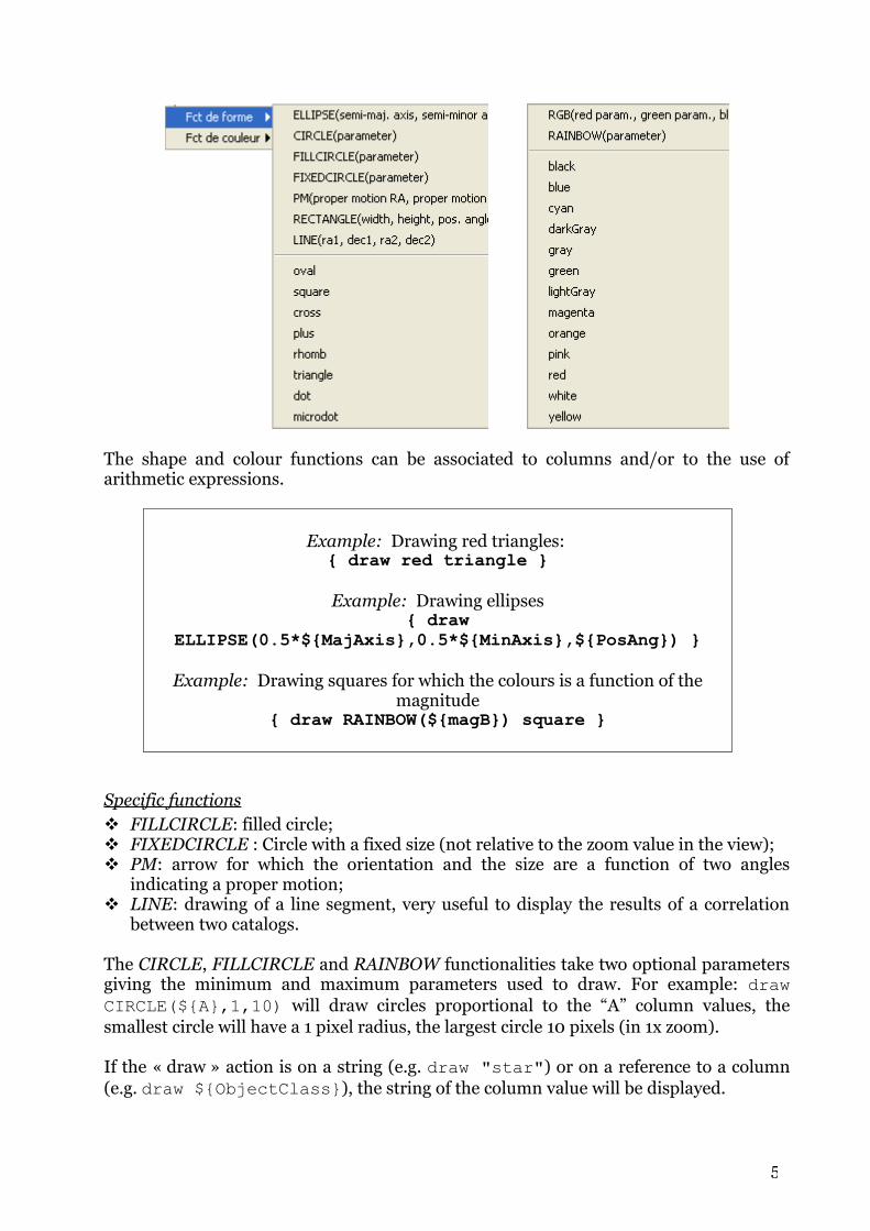
The shape and colour functions can be associated to columns and/or to the use of arithmetic expressions.

Example: Drawing red triangles: { draw red triangle }

Example: Drawing ellipses{ draw

ELLIPSE(0.5*${MajAxis},0.5*${MinAxis},${PosAng}) }

Example: Drawing squares for which the colours is a function of the magnitude

{ draw RAINBOW(${magB}) square }

Specific functions FILLCIRCLE: filled circle; FIXEDCIRCLE : Circle with a fixed size (not relative to the zoom value in the view); PM: arrow for which the orientation and the size are a function of two angles

indicating a proper motion; LINE: drawing of a line segment, very useful to display the results of a correlation

between two catalogs.

The CIRCLE, FILLCIRCLE and RAINBOW functionalities take two optional parameters giving the minimum and maximum parameters used to draw. For example: draw CIRCLE(${A},1,10) will draw circles proportional to the “A” column values, the smallest circle will have a 1 pixel radius, the largest circle 10 pixels (in 1x zoom).

If the « draw » action is on a string (e.g. draw "star") or on a reference to a column (e.g. draw ${ObjectClass}), the string of the column value will be displayed.

5

Column names or UCD The reference to a column name is usually done with the column name using the ${COLUMN_NAME} syntax. This method implies that the filter is more or less dedicated to a specific catalog since one needs to know explicitly the column names. In order to describe filters in a more generic manner, for example taking into account the magnitude independently of the column name given by the author, Aladin uses UCD.

UCDs or « Unified Content Descriptors » characterize columns independently of catalogs. For each column, a UCD was associated and gives you the physical quantity associated to the column. For example, a column with magnitudes will be labelled with the “pos.mag” UCD. The UCD’s list is maintained by an international committee and is available here: http://www.ivoa.net/Documents/latest/UCDlistMaintenance.html. Most of the astronomical servers give their catalogs in VOTable and already contain these valuable UCDs.

When a filtering rule uses a UCD, the used syntax is $[UCD]. Jokers characters ‘*’ et ‘ ?’ are authorized. For example, $[phot*] corresponds to the first column having a UCD that starts with « phot », that is the first column having magnitude measures.

In summary, referencing a column with its name is called with “{}” brackets while referencing a column with its UCD is called with “[]” brackets.

Example: Drawing a circle proportional to the magnitude for all sources brighter than 12

$[phot*]<12 { draw circle(-$[phot*]) }

In order to simplify references to columns, the edit board for filters offers two buttons « Columns » and « UCDs » that enable you to choose in a list the column name, or the UCD respectively, so that the corresponding text will be automatically written at the cursor’s location in the edition window.

5

If sources are selected in the view, and hence their measured are displayed, it is possible to select a column by a simple click on it in the measure panel. To do so, you need to choose the sub-menu « Pick… » when you click on « Columns » or « UCDs ».

Physical units Indicating physical units (e.g. arcmin, Jy, …) in the test enables you to get rid of the manual conversion for expressions using columns in which values are not expressed in the same unit. Units can be made as shown in the following example. This is a powerful example to describe generic filters.

Example: Drawing a circle proportional to the X flux (UCD : phot.flux;em.X-ray) for all sources for which the energy level is higher

than the given threshold$[phot.flux;em.X-ray]>10^-8 erg/m^2/s{ draw circle($[phot.flux;em.X-ray]) }

Modifying a filter

To find again a filter editing window, you need to select the corresponding filter in the stack and show its properties with the menu « Edit Properties ».

Extending the implementation of a filter

To be implemented, a filter has to be activated with the check close to its logo in the stack. By default, a filter is applied to all the catalogs planes that are below in the Aladin stack. However, if a filter is located in a directory in the stack, it will only be implemented to the catalog planes belonging to this directory.

5

Filter dedicated to a single specific catalog plane

Some servers offer a list of filters dedicated to their data (Simbad, NED, Skybot…). They appear in the data query form (c.f. 5.2 Server Selector) as a scrolling list at the end of the query parameters.

A dedicated filter, if activated does not appear in the stack and applies only to specific the catalog plane. It prevents any other generic filter to be implemented on this plane. The selection or activation of a dedicated filter can be modified afterwards through the “properties” associated to the plane (menu Edit Properties… ). Using the button « This filter on the stack for edition », it is also possible to change a dedicated filter in order to modify and/or apply it to several catalog planes.

Examples of generic filters

Circles as a function of magnitude

{ draw circle(-$[phot.mag*])}

Location Ellipses+Default display

{ draw ellipse( 0.5*$[phys.angSize.smajAxis], 0.5*$[phys.angSize.sminAxis], $[pos.posAng]) draw}

5

Blue squares for bright sources

$[phot.mag*]<17 { draw blue square}

Different colour symbols depending on the object type

$[src.class]="Star" {draw red square}$[src.class]="Radio" {draw blue rhomb}$[src.class]="Galaxy" || $[src.class]="Seyfert" {draw green plus}

Proper motions

{ draw pm( 5*$[pos.pm;pos.eq.ra], 5*$[pos.pm;pos.eq.dec])}

5.6Catalogs cross-match Button cross Menu: Catalog Cross match objects…

Aladin has an integrated cross-match tool for sources. The goal is to establish the shared sources between two catalogs. The cross-match tool will consider 2 catalog planes, do the correlation and generate a new catalog plane containing the shared sources.

The window controlling the cross-match can be access by the button « cross » or with the menu « Catalog Cross match objects ».

The three cross-match modes

Aladin has 3 cross-match modes that can be access with the tabs on top of the correlation window: A cross-match based only on the position; A cross-match “by field” based on identical values in a column of each catalog (e.g. an

identification); A cross-match based on the location, taking into account error ellipses.

5

Positional cross-matchThe positional cross-match board lets you give two catalogs, as well as the corresponding locations (ra, dec). If there is no ambiguity, column names will have been selected automatically by Aladin. It is then necessary to give the upper limit on the offset, or even the lower limit offset between sources to be cross-matched. It is given in arc seconds. Finally, the selector gives 3 choices:

1. When several objects are in the cross-match circle, only the closest sources will be cross-matched;

2. On the contrary, all possibilities will be kept;

3. Another possibility, all the sources with no counterparts will be kept.

Field cross-match (cross-ID)The cross-ID (or field cross-match) consists in the reunion of sources for which a value of a field is identical in both catalogs. This cross-match type is dedicated to a field that identifies each sources in a unique manner, e.g. an identification, a serial number, … In data bases, this is called « joint ».

Ellipses cross-matchThe board to control the ellipse cross-match is similar to the one for simple positional correlation. The main difference is the possibility to specify not only the columns for the position, but also the one for the errors on the position. This error should be expressed with 3 fields that define an ellipse: major axis, minor axis, and position angle with respect to the north.

Choosing the fields to keep

When Aladin performs a cross-match, a new catalog plane is created for the results. Each cross-match pair will correspond to a source in the resulting plane and by default; all the measures for the two corresponding sources will be kept. To avoid possible confusions on column names, they are automatically labelled with “_tab1” and “_tab2” respectively.

5

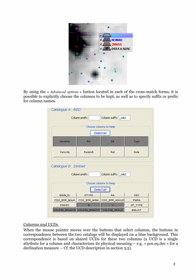
By using the « Advanced options » button located in each of the cross-match forms, it is possible to explicitly choose the columns to be kept, as well as to specify suffix or prefix for column names.

Columns and UCDs When the mouse pointer moves over the buttons that select columns, the buttons in correspondence between the two catalogs will be displayed on a blue background. This correspondence is based on shared UCDs for these two columns (a UCD is a single attribute for a column and characterizes its physical meaning – e.g. « pos.eq.dec » for a declination measure -- Cf. the UCD description in section 5.5).

6

Note: Some UCD should not appear more than one time in a table (« meta_main »). Hence, if the correspondence is displayed on a red background, it means that there is a conflict between UCDs. To avoid this, you need to click on the dominating column name by holding the Ctrl key. Without further indications, the first column from the first catalog will be dominating.

5.7 Column computer Menu: Catalog Add a new column …

Catalogs give some measures that can be seen in the « measures panel » by selecting the sources (cf. measures). These measures are displayed as different columns with values. Aladin gives you the opportunity to add columns, obtained by computing on the other columns values. For example, it is possible to create a « J-K » column giving the difference between two magnitude columns « J » and « K ».

Access to the window

The window to control the computing of a new column can be accessed either by the contextual menu in the « measures panel « (right click or CTRL click), or with the main menu « Catalog add a new column… ». In this last case, you need to specify beforehand the concerned catalog by selecting it in the stack.

General information on the new column

To create a new column, you need to specify a name. You can also add a unit for the new column, as well as the UCD that should be associated (cf. 5.5 using filters). You can also specify the number of decimals for displaying values.

6

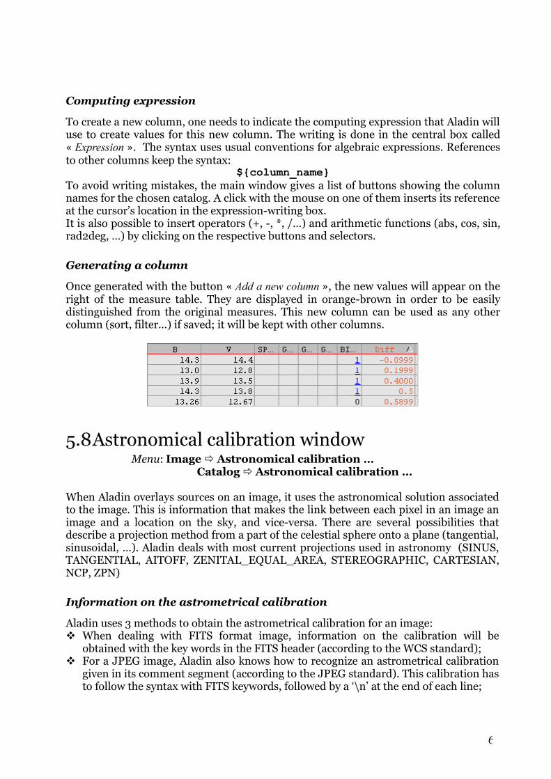
Computing expression

To create a new column, one needs to indicate the computing expression that Aladin will use to create values for this new column. The writing is done in the central box called « Expression ». The syntax uses usual conventions for algebraic expressions. References to other columns keep the syntax:

${column_name}To avoid writing mistakes, the main window gives a list of buttons showing the column names for the chosen catalog. A click with the mouse on one of them inserts its reference at the cursor’s location in the expression-writing box.It is also possible to insert operators (+, -, *, /…) and arithmetic functions (abs, cos, sin, rad2deg, …) by clicking on the respective buttons and selectors.

Generating a column

Once generated with the button « Add a new column », the new values will appear on the right of the measure table. They are displayed in orange-brown in order to be easily distinguished from the original measures. This new column can be used as any other column (sort, filter…) if saved; it will be kept with other columns.

5.8Astronomical calibration window Menu: Image Astronomical calibration …

Catalog Astronomical calibration …

When Aladin overlays sources on an image, it uses the astronomical solution associated to the image. This is information that makes the link between each pixel in an image an image and a location on the sky, and vice-versa. There are several possibilities that describe a projection method from a part of the celestial sphere onto a plane (tangential, sinusoidal, …). Aladin deals with most current projections used in astronomy (SINUS, TANGENTIAL, AITOFF, ZENITAL_EQUAL_AREA, STEREOGRAPHIC, CARTESIAN, NCP, ZPN)

Information on the astrometrical calibration

Aladin uses 3 methods to obtain the astrometrical calibration for an image: When dealing with FITS format image, information on the calibration will be

obtained with the key words in the FITS header (according to the WCS standard); For a JPEG image, Aladin also knows how to recognize an astrometrical calibration

given in its comment segment (according to the JPEG standard). This calibration has to follow the syntax with FITS keywords, followed by a ‘\n’ at the end of each line;

6

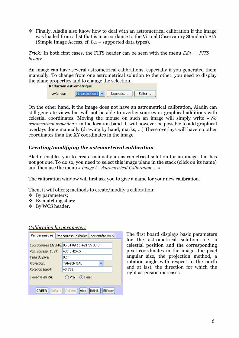
Finally, Aladin also know how to deal with an astrometrical calibration if the image was loaded from a list that is in accordance to the Virtual Observatory Standard: SIA (Simple Image Access, cf. 8.1 – supported data types).

Trick: In both first cases, the FITS header can be seen with the menu Edit FITS header.

An image can have several astrometrical calibrations, especially if you generated them manually. To change from one astrometrical solution to the other, you need to display the plane properties and to change the selection.

On the other hand, it the image does not have an astrometrical calibration, Aladin can still generate views but will not be able to overlay sources or graphical additions with celestial coordinates. Moving the mouse on such an image will simply write « No astrometrical reduction » in the location band. It will however be possible to add graphical overlays done manually (drawing by hand, marks, …) These overlays will have no other coordinates than the XY coordinates in the image.

Creating/modifying the astrometrical calibration

Aladin enables you to create manually an astrometrical solution for an image that has not got one. To do so, you need to select this image plane in the stack (click on its name) and then use the menu « Image Astrometrical Calibration … ».

The calibration window will first ask you to give a name for your new calibration.

Then, it will offer 3 methods to create/modify a calibration: By parameters; By matching stars; By WCS header.

Calibration by parametersThe first board displays basic parameters for the astrometrical solution, i.e. a celestial position and the corresponding pixel coordinates in the image, the pixel angular size, the projection method, a rotation angle with respect to the north and at last, the direction for which the right ascension increases

6

Calibration by WCS header The third board displays FITS keywords giving the parameters for the calibration in the WCS standard. If you know this standard, you can directly modify these parameters. It is for example possible to use the astrometrical solution from another image directly by copy/paste of its WCS parameters.

Trick: It is also possible to modify a value in a WCS keyword via the script command: set PlanID FITS:keyword=value (cf. – Aladin by script)

Calibration by matching starsThe second board displays a table used to write a list of XY image coordinates and their corresponding celestial coordinates. It is a powerful and flexible method to quickly obtain excellent calibrations. We will briefly describe this method here. For more details, please refer to the online tutorial dedicated to this manipulation (http://aladin.u-strasbg.fr/tutorials/aladin.gml).

Let’s assume that we loaded in the left view, a JPEG image that is not calibrated, and a DSS image of the same field, with an astrometrical catalog like UCAC2 overlaid in the right view. The method to calibrate the JPEG image is to click successively on a star in the non-calibrated image, and then on the corresponding UCAC2 source. For each click with the mouse, Aladin fills the table in the calibration board. Four corresponding measures are usually enough to get a good calibration.

Note: When one needs to get the coordinates for a start by clicking with the mouse, Aladin uses an algorithm with a barycentre centroid. If it is not possible to determine the

6

centre (too wide a star), a message will be display to say that the clicked location will be taken as it is.

Tricks: It can be useful to perform the “symmetry” of the DSS image in order to get closer to

the orientation of the image to calibrate ( Image Symmetry ) It is better to only display the bright stars with little proper motion. Using a filter an

a catalog ease the pointing of corresponding sources, for example: $[pos.pm;pos.eq.dec]<3 mas/yr && $[pos.pm;pos.eq.ra]<3 mas/yr && $[phot.mag*]<17 { draw circle(-$[phot.mag*]) }

It is possible not to load a catalog; the celestial coordinates will then be those deduced for the DSS image calibration. The calibration precision will then be lower.

Using the translucence (Menu « image Transparency level ») to visualise the image that just got calibrated, onto the DSS image, lets you check simply the quality of the calibration.

Redo and undoDuring the creation process or the adjustment of the calibration, it is possible to go back to the former solution by using the « Redo » and « Undo » buttons at the bottom of the window.

Calibration of a catalog

Aladin also offers the possibility to calibrate or recalibrate a catalog. This corresponds to the computation, for each source, of its celestial position. Select the catalog plane in the stack and use the menu « Catalog Astrometrical Calibration… ». The interface and methods are the same as for the image.

Moving with the mouseIf you are using the calibration method by parameters (1st board), it is possible to move directly the sources from a catalog to calibrate in the view in order to visualise the result directly. For this you need to click and move a source with the mouse; the other sources will follow. Along the move, the calibration parameters will be automatically adjusted. The move is validated with the « CREATE » or « MODIFY » button which computes the new celestial positions according to the indicated offset.

6

Catalog with only XY positionsIf you load a table or catalog without celestial positions but with two columns representing the XY coordinates that Aladin could detect (based on the column names and/or the attached UCDs), the calibration window of the catalog is instantaneously opened, inviting you to create a calibration for these sources.

Saving a recalibrated catalogOnce you save a catalog, after its recalibration, Aladin systematically adds two columns with the celestial position for each source.

5.9RGB colour image builder Icon: rgbMenu: Image RGB image builder…

Aladin can build a true colour image from 2 or 3 images with grey levels. To do so, the first component will be affected to the red colour, and the second and third images will be affected to green and blue components respectively. The true colour image will be saved in a plane of the stack.

Trick: If the mouse cursor is on the RGB plane logo that was created, the 3 logos for the 3 original images appear with the colour of their respective component.

Resampling

In order to have the image pixels corresponding to the same locations on the sky, Aladin does a resampling on two of the images according to the astrometrical position in the third one. This image is then called the « reference image ». By default, the reference image will be the image for which the angular pixel size is the smallest. This resampling is based on the « nearest neighbour pixel » algorithm (cf. - resampling)

Access to the window

The window to generate a colour image can be accessed either with the menu « Image Create a RGB image… » or with the « rgb » button.

The default choice of the images for each component depends on the state of the stack. If there are only two or three selected planes, Aladin will use them to

6

fill the form, else Aladin will take the 3 images on top of the stack, or else the 2 first ones. If the image associated wavelengths are known, Aladin will sort them according to this parameter

Specific case for 2 images

It is possible to only select 2 images. In such a case, the 3rd colour component will be computed according to the 2 other by taking the average of the two other images. This method builds very nice colour images if the free component is the green colour (default mode).

2 images differences With 2 images, it is also possible to do a colored subtraction. The positive differences will be the values from the first colour component; the negative differences will be those for the second colour component. Furthermore, the differences will be normalized between 0 and 255 to give a maximum contrast. This method is interesting to visualise variations in a quick way, even small ones, between two images.

5.10 Images associations: cubes and mosaics Icon: assocMenu: Image Mosaic image builder…

Image Blink/Movie generator…

Aladin can associate 2 or more images by combining them either as a cube that will be displayed as an animated sequence, or by creating a new mosaic image from the original images.

Access to the association window

The window can be opened either with the menu « Image Mosaic image builder » or « Image Blink/Movie generator », or else with the « assoc » button, and lets you control the association. You can indicate the original image planes, the initial sequence delay in the case of producing a cube, and the reference image if resampling is needed pour superimposed pixels.

Mosaic

When producing a mosaic image, the image obtained will have the required size in order to contain all the original images in the projection grid from the reference image. The image obtained will be displayed and can be

6

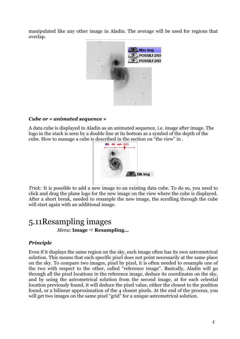
manipulated like any other image in Aladin. The average will be used for regions that overlap.

Cube or « animated sequence »

A data cube is displayed in Aladin as an animated sequence, i.e. image after image. The logo in the stack is seen by a double line at its bottom as a symbol of the depth of the cube. How to manage a cube is described in the section on “the view” in .

Trick: It is possible to add a new image to an existing data cube. To do so, you need to click and drag the plane logo for the new image on the view where the cube is displayed. After a short break, needed to resample the new image, the scrolling through the cube will start again with an additional image.

5.11Resampling imagesMenu: Image Resampling…

Principle

Even if it displays the same region on the sky, each image often has its own astrometrical solution. This means that each specific pixel does not point necessarily at the same place on the sky. To compare two images, pixel by pixel, it is often needed to resample one of the two with respect to the other, called “reference image”. Basically, Aladin will go through all the pixel locations in the reference image, deduce its coordinates on the sky, and by using the astrometrical solution from the second image, at for each celestial location previously found, it will deduce the pixel value, either the closest to the position found, or a bilinear approximation of the 4 closest pixels. At the end of the process, you will get two images on the same pixel “grid” for a unique astrometrical solution.

6

Access to the window

The window controlling the resampling can be opened with the menu « Image Resampling ». You need to select beforehand the image to resample in the stack. In the window, you need to specify the reference image, whether you wish to keep or not the “full” pixels, or just the “grey levels” code on 8 bits (quicker), choose the estimation method for the pixel values and at the end, say whether the original image needs to be replaced by the newly sampled image, or kept in the stack.

Attention: Please note that the resampling methods in Aladin do no preserve the flux, i.e. the sum of the pixel values before the resampling is not the same as the one afterwards.

Note: An image that was resampled shows the following logo in the view:

Trick: Using the translucence of images (cf. ) is a quicker and more flexible alternative to resampling. It is however less precise since it does not act pixel-by-pixel, but only based on the four corners and does a global approximation for the other pixels location.

5.12Arithmetic operations on images Menu: Image Arithmetic operations …

Image ConvolutionImage Pixel normalisation [0..1]

Addition, subtraction, multiplication and division

Aladin offers a simple interface to compute simple basic operations on a couple of images: addition, subtraction, multiplication, and division. The control window can be opened with the menu « Image Arithmetic operations » (accessed only if at least two images are in the stack). Aladin will

proceed pixel by pixel by doing, if needed, a resampling of the second image so that it corresponds to the grid of the first image (cf. 5.11). One can ask to do first a normalisation of the pixels in the two images so that their values are located between 0 and 1 (real format). The result from the operation will be seen as a new image plane in the pile.

Trick: If you wish to use a scalar as the second operant rather that an image –e.g. add a given value to all pixels – you can use scripts commands: +, -, *, /(cf. )

6

Convolution

Furthermore, the menu « Image Convolution … » lets you “convolve” the current image with a specific array, i.e. to compute a new image according to the product of each pixel from the original image (and their neighbours) with a specific array. The sub-menu gives the array usually used in astronomy (Gauss, Mex, TopHat…) with different sizes. You can also define you own convolution matrix by using the script command: « conv » (cf. ). The resulting image will replace the original one in the stack. If you wish to keep the original image, you need to duplicate it beforehand (menu: « Image Duplicate the image plane »)

5.13Save, export and print Icon: Menu: File Save…, File Export…

File Backup…, File Print…Short key: Ctrl +S, Ctrl +P

By using the icon on the top left corner, below the menu band, representing a floppy disk, you can open the save and export window. You an also use the different possibilities from the « file » menu

to get directly the desired action.

Aladin has several possibilities to save your work: Printing the view(s); Save the current view. The supported formats are BMP, JPEG, PNG and EPS. This

last format is especially preferred for a scientific publication; Backup the stack and views for a further use; Exporting one or several planes in the stack. The images will be exported in FITS or

JPEG (for colour images), catalogs in TSV (Tab-Separated-Value) or VOTable (cf. 8.2);

Access to URL that gave the images and catalogs.

7

Generate a “clickable” map

When save the Aladin view, the format « PNG+LINK » is offered. This format is dedicated to the creation of « Web clickable maps ». The view is save with the classical PNG format. A second file is generated simultaneously with a “.lnk” extension. It contains an ASCII format that is very simple for clickable objects present in the view, their position in the PNG image and a URL to access to the whole associated record. Both files are located on a web server and will let you build easily a clickable map. For more details on the method, the format and implementation examples, please go to: http://aladin.u-strasbg.fr/java/FAQ.htx#Map

5.14User preferences Menu: Edit User preferences …

Aladin gathers in the preference window, most of the configuration parameters specific to the user. You can hence define the following elements: The default directory where Aladin will look for or save local files; The language for the graphical interface (english, french, italian,); The default display mode for pixels (inversed video, colour table, …); When loading an ASCII table, the character used to separate columns (TAB, ‘ ;’, …) ; Activation or not of dedicated filters (cf. 5.5 – filter usage); Translucence level for instrumental fields (cf. 5.2.6 - FoV) by default; The default image server (when querying with a simple astronomical object name); The default web site is the server directory (cf. 5.2.1 – the server selector), i.e. the

machine that will give at each start the list of available servers, the parameters to give, … ;

According to your computer configuration, your preferred browser for the web;

7

The starting mode for Aladin, e.g. « astronomer » for professionals, « undergraduate » for scholars or a simple dynamic visualisation window (« preview ») (cf.).

The preference window lets you also: Create your own translation language (see below); Reload during the session all the data server definitions, which will also reinitialise

the internal cash for Aladin metadata.

Some parameters are not tuneable, but can be simply kept from one session to the other, for example the size and location of the Aladin window, the reticule type (large or classical), the activation or not of info-bubbles on sources …

Trick: The configuration parameters are kept in simple ASCII file « Aladin.conf » that can be edited in the « .aladin » directory on your home directory ($HOME en unix, \Document and Settings\YourName in Windows). To reinitialize the parameters to the original configuration, you only need to delete this file.

Interface language management

Aladin does support several languages for its graphical interface. It is possible to create your own translation if the language you wish to have is not yet supported. To do so, use the « New translation?» button and specify – in English 00 you language and the “2 letter” code that corresponds to it (e.g. “French” –“fr”). Aladin will open an editing window that displays all expression that need to be translated (en English), those that were already translated if some exist and those that are not necessary anymore (used by a former version for example). You can install your translation that will appear in the next session as a possible language alternative in the supported translation list.

Details: Expressions that are not translated will appear in english. Aladin supports non-ASCII languages (e.g. Chinese) and eventually written from

right to left (e.g. Persian). It is possible to complete or translate an existing translation. To do so, you first need

to load this language, then to press the “new translation” button while keeping the “language” and “2 letter code” empty. Your additions to the translation will only apply to your Aladin installation.

Note: If you wish, you can contact the CDS and the Aladin development team in order to have the whole user community benefit from your work. Your translation file will be saved in the same directory as the configuration file for Aladin (see above) with the name « Aladin-language-version-perso.string… ».

5.15 The script console Menu: Tool Script consol …Short key: F5

7

All the actions that can be done with the graphical interface can also be done with « online commands ». The goal is to be able to use Aladin in « script » mode to do repeatable works, indicate treatments to do, or control Aladin remotely.

These commands can be submitted through different channels among which: The main entry The « script console »

The script console is opened with the menu « Tool script console… ». This window shows in bracket all the commands equivalent to the action that was done in the graphical interface. This is a useful help to learn the syntax. It is possible to type directly a command after the « Command> » prompt. The UP and DOWN arrows let you scroll through the already submitted commands in order to re-edit them, modify them or execute them again.

Trick: Be careful always write after the « Command> » prompt. If it is not displayed, press the Enter key to get a new line.

Alternative to the console

To rapidly give a command without opening the console, it is possible to type it directly in the location field used by Aladin to indicate the current position under the mouse.

Please refer to the “Aladin by script” section (cf. , below) for more information on the control of Aladin in script mode.

6 Additional ToolsAladin provides access to a number of supplemental tools: The Simbad pointer for automatic SIMBAD identification of objects of interest A capability for using macros for repetitive tasks A mechanism for interacting with other astronomy tools compatible with Virtual

Observatory messaging standards A tool for extracting sources from images : S-extractor A labels generator

Each of these tools is breifly described below.

7

6.1 Simbad Pointer

Menu : Tools Simbad automatic pointer

To aid the exploration of an image, activate the Simbad pointer which starts a continuous connection with the Simbad database.When your mouse remains over the same location in the image for a few moments, Aladin queries the Simbad database and returns a short list of information about objects at that position (the principle identifier, the object type, the spectral type...). The criteria used in selecting information from the database is based on the number of bibliographic references. Note: If a Simbad has already been performed with the result is available as a catalogue plane, then Aladin will use this information to avoid multiple queries to Simbad.

6.2The Macro Controller

Menu : Tools Macro Controller

To facilitate repetitive tasks Aladin provides a macro controller which is based on Aladin script commands (see 7.1). It allows for the script commands to include input variables that allow for the execution of a set of commands for a list of object names.

The macro controller window is divided into 3 parts : The top panel allows the input of a script. The variables can be specified as $1, $2 etc. The middle panel allows the input of lists of values to be taken by the variables. The lower panel controls the execution of the script.

The script and the input values for the variables may be saved for future use by using the File menu of the macro controller window. File-> Save Script

Hint : When writing a script, Aladin automically recognises the syntax and colours the various elements of the scriptto ease the editing. The commands are also ‘clickable’ to provide immediate help .

7

6.3Interaction with VO tools: Plastic/SAMP

Menu : Tools VO Tools

Aladin provides a mechanism for connecting to other independent applications, for example to tools that provide plotting capabilities, or for the display of spectra. This is achieved through use of the VO Plastic/SAMP messaging standard.

The Principles of Plastic/SAMP

PLASTIC/SAMP permits a dialog between applications so they may send data between them, but also so that they may interact. For example the selection of a source, or set of sources in Aladin also triggers their immediate selection or highlighting in other tools.

Configuration of VO Tools

Aladin facilitates the use of PLASTIC with a window that presents a list of applications that may be ‘connected interoperably’ with Aladin. This window provides a way of easily installing other applications, that will then be listed in the Tools -> VO Tools menu. the list of tools in=s managed dynamically so that it includes the latest versions of those applications.

7

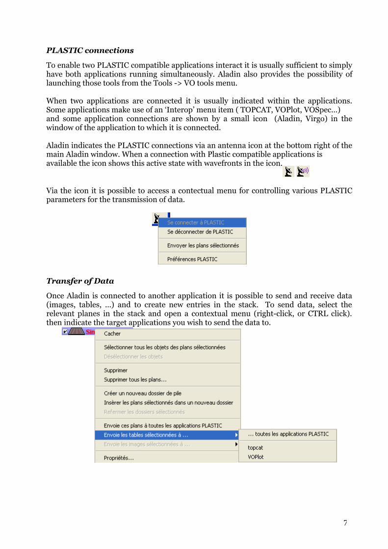
PLASTIC connections

To enable two PLASTIC compatible applications interact it is usually sufficient to simply have both applications running simultaneously. Aladin also provides the possibility of launching those tools from the Tools -> VO tools menu.

When two applications are connected it is usually indicated within the applications. Some applications make use of an ‘Interop’ menu item ( TOPCAT, VOPlot, VOSpec…) and some application connections are shown by a small icon (Aladin, Virgo) in the window of the application to which it is connected.

Aladin indicates the PLASTIC connections via an antenna icon at the bottom right of the main Aladin window. When a connection with Plastic compatible applications is available the icon shows this active state with wavefronts in the icon.

Via the icon it is possible to access a contectual menu for controlling various PLASTIC parameters for the transmission of data.

Transfer of Data

Once Aladin is connected to another application it is possible to send and receive data (images, tables, ...) and to create new entries in the stack. To send data, select the relevant planes in the stack and open a contextual menu (right-click, or CTRL click). then indicate the target applications you wish to send the data to.

7

Interactions

Generally, when the data are tables or catalogues, the sources selected in one of the applications are automatically selected in the other application. It is a very practical method for example, to show the distribution of source selected, say in a colour-colour diagram in VOPlot, on the sky.

Note : The PLASTIC actions are dependent on the applications, and it is possible that a selection of an object is simply ignored by a PLASTIC compatibel application. Indeed some applications allow for configuration of the PLASTIC interoperability behaviours.

6.4Extraction of sources via SExtractor

Menu : Tools Remote Tools S-extractor…

Aladin does not natively include tools for photometry, rather it provides a mechanism to call Sextractor which is designed for source extraction including calculation of magnitudes of the sources (Bertin & Arnouts – 1996).

The Tools -> Remote Tools -> Sextractor menu opens the Server Selector window, with a number of Sextractor options. This includes selection of the reference image which should be used, and various filters to be applied to the output when displaying the results, for example to display circles around in source with radii in proportion to their brightness.

7

Once the options are selected and the submit button is pressed the Sextractor 'remote tool' which is an installation of Sextractor on a cluster of compueters in Strasbourg will execute the calculation and send the result back and it appears as a new plane in the stack, and shows the result overlaid on the image.

Note : If the image is local (stored on your disk) it may be neccesary to authorize the remote application to temporarily use a particular network port of your machine so that it may access the image. There may also be further complications with your network provider when using loal images in this way. Using images on external servers however should work with out problems of this kind.

6.5Generating 'thumbnail' images

Menu : Image Thumbnail generator

Aladin provides a way of easily generating 'thumbnail images' for a list of objects, that is a set of small images (cut out from a larger image in the stack) centred on all of the objects in a list. The list may be defined by a selection of objects in a catalogue plane of the stack, or as a set of interactively 'tagged' objects. Aladin will generate as many views (see 5.1.2) as there are objects in the list.

Example:

Suppose you wish to create thumbnail images of all the objects that may be planetary nebulae in the central region of the field of the comas cluster: Load a DSS of the field, and overlay a Simbad

plane Select sources that are indicated as possible

Planetary Nebulaeby using the search box in the lower right of the main wondow. Simply type « PN? » in the text box and press GO. This selects all sources indicated as PN? in the Simbad plane.

7

Creat thumbnail images of all these sources via the Image->Thumbnail view generator menu item

The generated thumbnail views are automatically 'locked', which means that they do not zoom or pan in concert with other views, this is indicated by the small padlock symbol in the lower left of each thumnail view (see 5.1.2 – locked views).

Hint : Thumnail views may be deleted individually (as for any view), and also all of the 'locked' views may be deleted at one time both these options are available by right-clicking on a view.

Hint : When scrolling though the many views that may be generated by the above procedure, it is often useful to 'stick' the full field view, so that it remains visible as the thumnail views are scrolled.

Thumbnail views of multiple images

Thumbnails may be generated simultaneously for a number of bands, and be displayed side by side. For example to compare the thumbnail images for a set of sources in two images, first select the views of the two images, then select the desired sources and generate the thumbnails with Image-> thumbnail view generator. The resulting thumbnails will be arranged so that the thumbnails from the two images are shown side by side. The multi-view options can be altered to facilitate the comparison, in this case the 2x1 and 2x2 views are convenient.

7 Aladin for expertsIn this section we briefly outline some of the advanced features of Aladin. These include:

How to use Aladin in script mode; How to use aladin as an applet; Extending the capabilities by developing java plugins for Aladin; How to use IDL with Aladin

7

7.1 Aladin script modeAs an alternative to the graphical interface, Aladin may be controlled by contextual commands. The commands may be entered interactively at the command line, or be uploaded via a file containing the script commands. The script commands may also be issued to Aladin via another program.

The various ways of using script commands

Script commands may be used in various different contexts:

An alternative to using the mouse To control Aladin 'remotely' using another program via:

Standard input, a shell script, or other scripting languages like perl the « execCommand(String) » method so that another application sharing the same

java virtual machine (JVM) can interact with Aladin (see - http://aladin.u-strasbg.fr/java/FAQ.htx#Launch)

the « execAsyncCommand(String) » method to control aladin in applet mode using JavaScript.

How to launch an Aladin applet To write macros

Example script

Example : Download an image from a URL, add a SIMBAD plane, activate the display of a coordinate grid, and specify a colour table (BB) for the

display:get File(http://monServeur/monImage.fits)

syncget Simbadgrid on

cm bb noreverse

The list of Aladin script commands

Help on the script commands may be obtained via the « Help -> Help on script commands » menu item. This displays the online help in the main Aladin window. Each script command may be clicked to provide an explanation of the command and the input parameters.

8

Using the planes of the stack as 'variables'

In the context of a script, it is possible to use the planes of the stack as variables. The planes may be referred to by name, or by their position in the stack. Also, script commands may create new planes of the stack « PlaneName = commande… » . To refer to the planes by position in the stack « PlaneName» may be replaced by @nnn where nnn is the the number of the plane - @1 being the lowest plane in the stack. If the plane with the specified number already exists, a new plane will be created at the top of the stack.

Example : Create a plane called « MyImage » with an DSS/ESO image of M1:

MyImage = get ESO(DSS1) M1

This method is very practical when the script includes artithmetic operations on image planes in the stack (addition, subtraction, multiplication, normalisation, convolution…).

Example : Make an image of the difference of 2 images in J and F bands :A = get Aladin(J) M1B = get Aladin(F) M1

Diff = A – B

8

7.2Make your data visible in the Aladin applet

As indicated in section 2, Aladin may be used as an extension of a web browser (IExplorer, Firefox, Mozilla …) as a java applet. This method allows data providers to allow thier users to automatically visualise data (images and catalogues) in Aladin without having to download or install the software.

Launching an Aladin applet

To start an Aladin applet reuqires simply calling a URL. There are many sites which use Aladin in this way (see 2 - Aladin en applet)

Hint : By default, Aladin will start up within the web page. It is also possible to launch the applet in a separate window, or in a simple 'preview' mode (cf. 5.1.2 – preview). For details consult the FAQ http://aladin.u-strasbg.fr/java/FAQ.htx#startapplet .

Controlling the Aladin applet

To show the desired data in the Aladin applet, it is necessary to control it via script commands. The script is input via the « -script » parameter in the URL that calls the applet, or as an input to a JavaScript method.

The « -script » parameter The URL dused to call the applet accepts a parameter of the form ’ « -script=xxxx » where « xxx » is an Aladin script. The script may consist of multiple commands separated by a semi-colon ‘ ;’. The script is executed immediately after the applet is launched, and permits loading of data for visualisation.

Example : Start the applet with data from a specified file and overlay a coordinate grid

http://.../nph-aladin.pl?-script=get+File(http://xxx);grid+on

Hint : The Aladin web pages provide a formula to assist the generation of well formed URLs for calling the applet with various functons. See - http://aladin.u-strasbg.fr/java/nph-aladin.pl?frame=form

Using JavaScriptAladin in applet mode may also be controlled via a JavaScript function with the following reference:

document.aladin.execAsyncCommand(script)

8

In contrast to the pervious method, the use of the « -script » parameter with JavaScript allows modification of the behaviour of the Aladin applet. It is not neccessary to restart Aladin for each new data set to be visualised.

For more information about controlling Aladin via JavaScript, refer to the FAQ (http://aladin.u-strasbg.fr/java/FAQ.htx#JavaScript). And for more general information on how to provide your data Aladin see - http://aladin.u-strasbg.fr/java/HowToProvideMyData.htx .

7.3Aladin extensions: « plugins »Menu : Tools Plugins…

Aladin is written in the Java programming language, and it is possible to add extensions written in Java to extend the capabilities.

Installing plugins

The installation of plugins is done by the Plugin Controller accessible in the menu : « Tools Plugins Plugins controller ». This opens a window that shows all the installed plugins. The « Download » button shows the available plugins on the official Aladin site.

The plugins must be installed in compiled form (.class ou .jar), in the « .aladin/Plugins » directory in your home area ($HOME on Unix, \document and Settings\yourName on Windows). After downloading, it is necessary to click the Après les avoir copiés à cet emplacement, il est nécessaire de cliquer sur le bouton « Re-load » button.

8

Writing Aladin plugins

Writing plugins requires a reasonable understanding of the Java language. It involved extending the « AladinPlugin » object class in order to access the methods required for manipulation of the stack, and handling of images and catalogues.

The documentation for creating plugins is available http://aladin.u-strasbg.fr/java/FAQ.htx#plugins.

7.4Interactions IDL / AladinIDL (Interactive Data Language) is a language and environment which is often used for image processing, with a significant astronomer user community. An set of IDL procedures (.pro files) which allow the use of Aladin with the IDL environment are available at http://aladin.u-strasbg.fr/java/idl_aladin_interface.tar.gz . These allow the use and exchange of images, tables, colour tables, etc. between Aladin and IDL.

For more information on the use of Aladin libraries for IDL see - : http://aladin.u-strasbg.fr/java/FAQ.htx#IDL.

8 Using AladinThe Aladin software has evolved for more than 10 years. a wealth of practical information can be found in the FAQ http://aladin.u-strasbg.fr/java/FAQ.htx. This document is continually updated as new functions are added. there are also numerous tutorials and practical examples on-line, and is a good ressource for students. (http://aladin.u-strasbg.fr/tutorials/aladin.gml).

The following sections present some notes on the varu=ious uses of Aladin. For more information please refer to the FAQ mentioned above.

8.1 User profilesAladin provides a large number of options and functions for manipulating images and catalogues with a relatively complex graphical interface. It is possible to change the interface to accomodate the needs of users who may have different needs, and to provide a simpler interface (if desired) for first time users.

Aladin est un logiciel qui permet un grand nombre de manipulations sur les images et sur les catalogues. Afin de permettre une prise en main plus facile pour les utilisateurs débutants, il peut être démarré en profil « undergraduate ». Dans ce mode, seules les fonctions de base sont accessibles dans les menus et dans la barre des outils. D’autre part, Aladin peut être également utilisé pour de simple « visualisation » d’images et catalogues sans proposer à l’utilisateur l’ensemble des possibilités de l’interface graphique. Pour cela Aladin peut être démarré en profil « preview ». Dans ce mode, Aladin n’affiche que la vue courante, sans les autres panneaux de la fenêtre principale.

Le profil de démarrage se configure via la fenêtre des « préférences utilisateurs » (cf. 5.14).

8

Pour démarrer selon le profil « undergraduate » il est également possible de spécifier le paramètre « -outreach » sur la ligne de commande d’Aladin. Dans ce cas, l’étudiant n’a pas la possibilité de changer de profil en cours de session.

De même l’utilisation du paramètre « -preview » démarrera Aladin selon le profil « preview » c'est-à-dire « simple fenêtre » (cf. – plein écran et simple fenêtre). La touche ESC permet de faire réapparaître les éléments manquants de l’interface.

Astuce : En mode « preview », Aladin permet de visualiser très facilement des images couleurs, non nécessairement astronomiques. La fonction glisser/déplacer permet de charger en un clic une image issue d’un navigateur Web ou du gestionnaire de fichiers, les fonctions de zoom et de déplacement en font un outil très souple pour la consultation de photos.

8.2Les types de données supportésAladin supporte la plupart des formats utilisés en astronomie que ce soit pour les images, pour les catalogues ou pour les « groupements » de données. D’autre part, il prend en compte les algorithmes de compression les plus répandus.

Format Type de données VisuAladin Commentaires

FITS Image [+ WCS] Pas de limite de tailleJPEG Image couleur [+WCS] < 100 Megapixels1

GIF Image couleurPNG Image couleur

HCOMP Compression image FITS

Applicable sur les images FITS uniquement

FITS- RGB Image [+WCS]FITS-CUBE Cube d’images [+WCS] <1024x512x512

FITS-RICE Compression image FITS

Applicable sur les images FITS uniquement

ASTRORES Catalogue Prédécesseur de VOTable, (supporté pour compatibilité)

VOTABLE CatalogueStandard IVOA totalement supporté (base64,FITS…)<1 million de sources

FITS-ST Catalogue Table FITS en ASCII<1 million de sources

FITS-SB Catalogue Table FITS en binaire<1 million de sources

1 Sur la base d’une machine disposant d’1Gigaoctets de RAM

8

CSV & TSV Catalogue “Character separated value”<1 million de sources

BSV Catalogue “Blank separated value”<1 million de sources

SEXTRACTOR Catalogue Format par défaut de S-extractor

MFITS Données multiples FITS multiples extensionsAJ Pile Aladin Sauvegarde de la pileAJS Script Aladin Fichier de commandes scripts

FOV Champ de vue Description de champs de vue instrumental (note IVOA)

IDHA Liste d’images Concurrent de SIA, (supporté pour compatibilité)

SIA Liste d’images [+WCS] Standard IVOA(< 10 000 lignes)

SSA Liste de spectres Standard IVOA(< 10 000 lignes)

GZIP Compression Applicable sur tous les autres formats

Aladin reconnaît automatiquement la nature des données en se basant sur le contenu : l’extension du nom de fichier ou la présence d’un « Content-type » pour un flux http n’ont pas d’incidence sur la reconnaissance du fichier.

Exception : Le format AJS (script Aladin) est une exception car sa nature ne peut être reconnu de façon automatique sans risque de confusion. Pour lever l’ambiguïté, Aladin se basera sur l’extension de fichier « .ajs » et/ou sur la présence en première ligne du commentaire suivant : « #AJS ».

8.3Standard FITS et calibration astrométriquePour la calibration astrométrique, Aladin suit le standard FITS officiel : le premier pixel en bas à gauche est numéroté (1,1) et la position céleste correspondante est centrée sur le pixel. Concrètement, la coordonnée en bas à gauche du premier pixel est donc (0.5,0.5).

A noter : IDL ne suit pas le standard FITS officiel, la coordonnée en bas à gauche du premier pixel est (0,0).

Aladin reconnaît plusieurs méthodes de calibrations : WCS standard, ancienne méthode DSS1, … ainsi que la plupart des projections courantes.

8.4Performances et contraintes techniquesLe développement d’Aladin a suivi deux règles :

1. Garantir la meilleure compatibilité possible avec le matériel et les systèmes d’exploitation existants,

2. Offrir les meilleures performances possibles dans ce contexte

8

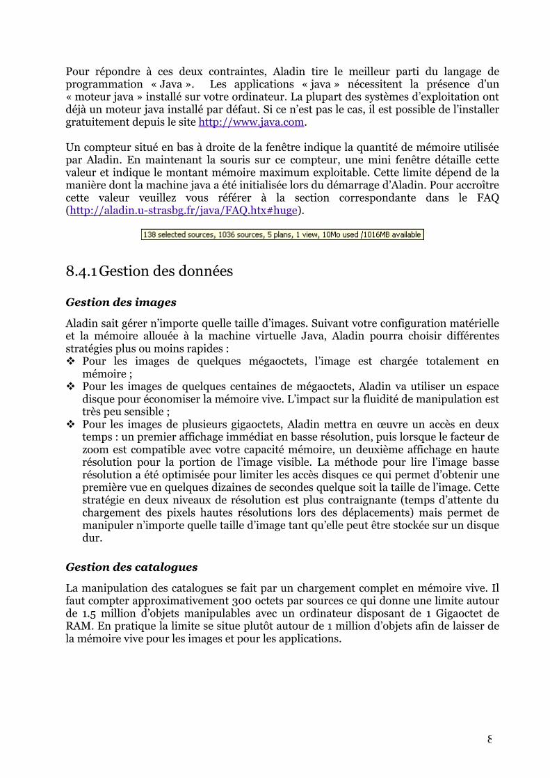
Pour répondre à ces deux contraintes, Aladin tire le meilleur parti du langage de programmation « Java ». Les applications « java » nécessitent la présence d’un « moteur java » installé sur votre ordinateur. La plupart des systèmes d’exploitation ont déjà un moteur java installé par défaut. Si ce n’est pas le cas, il est possible de l’installer gratuitement depuis le site http://www.java.com.

Un compteur situé en bas à droite de la fenêtre indique la quantité de mémoire utilisée par Aladin. En maintenant la souris sur ce compteur, une mini fenêtre détaille cette valeur et indique le montant mémoire maximum exploitable. Cette limite dépend de la manière dont la machine java a été initialisée lors du démarrage d’Aladin. Pour accroître cette valeur veuillez vous référer à la section correspondante dans le FAQ (http://aladin.u-strasbg.fr/java/FAQ.htx#huge).

8.4.1 Gestion des données

Gestion des images

Aladin sait gérer n’importe quelle taille d’images. Suivant votre configuration matérielle et la mémoire allouée à la machine virtuelle Java, Aladin pourra choisir différentes stratégies plus ou moins rapides : Pour les images de quelques mégaoctets, l’image est chargée totalement en

mémoire ; Pour les images de quelques centaines de mégaoctets, Aladin va utiliser un espace

disque pour économiser la mémoire vive. L’impact sur la fluidité de manipulation est très peu sensible ;

Pour les images de plusieurs gigaoctets, Aladin mettra en œuvre un accès en deux temps : un premier affichage immédiat en basse résolution, puis lorsque le facteur de zoom est compatible avec votre capacité mémoire, un deuxième affichage en haute résolution pour la portion de l’image visible. La méthode pour lire l’image basse résolution a été optimisée pour limiter les accès disques ce qui permet d’obtenir une première vue en quelques dizaines de secondes quelque soit la taille de l’image. Cette stratégie en deux niveaux de résolution est plus contraignante (temps d’attente du chargement des pixels hautes résolutions lors des déplacements) mais permet de manipuler n’importe quelle taille d’image tant qu’elle peut être stockée sur un disque dur.

Gestion des catalogues

La manipulation des catalogues se fait par un chargement complet en mémoire vive. Il faut compter approximativement 300 octets par sources ce qui donne une limite autour de 1.5 million d’objets manipulables avec un ordinateur disposant de 1 Gigaoctet de RAM. En pratique la limite se situe plutôt autour de 1 million d’objets afin de laisser de la mémoire vive pour les images et pour les applications.

8

8.4.2Le « cache » d’Aladin

Pour gérer au mieux les lenteurs inhérentes au réseau et pour économiser la mémoire vive, Aladin utilise un répertoire « cache » sur votre disque local nommé « .aladin ». Il se situe dans votre répertoire d’accueil ($HOME sous Unix, \Documents and Settings\YourName sous Windows). Il est constitué de plusieurs sous répertoires et de quelques fichiers que nous allons brièvement décrire.

« Aladin.conf » - La configuration Le fichier « Aladin.conf » mémorise vos préférences. La disparition de ce fichier rétablit les valeurs par défaut.

« Aladin-xxxx.string » - Les langues Le fichier « Aladin-xxxx.string » contient la dernière traduction utilisée (hors anglais et français). Ce fichier sera remplacé par une nouvelle traduction le cas échéant. Les fichiers dont le nom finit par la sous chaîne « perso » contiennent vos traductions personnelles, ils ne sont jamais effacés par Aladin.

« Cache » - pour les informations générales Les informations générales dont Aladin à besoin pour connaître les différents serveurs de données disponibles sont stockées dans le sous répertoire « Cache ». Elles servent notamment à la création de la fenêtre du « sélecteur de serveurs » (cf. 5.2). Ces fichiers seront utilisés tels que pour ne pas ralentir le démarrage de la prochaine session. Le cas échéant, ils seront mis à jour quelques secondes après le démarrage de la session Aladin.Le nom des fichiers est basé sur l’URL qui a fourni l’information mais dont certains caractères ont dû être encodés pour être acceptés en tant que nom de fichier. La suppression manuelle de ces fichiers ralentira simplement le démarrage de la prochaine session.

« Plugins » – pour les plugins Le sous répertoire « Plugins » contient toutes les extensions java apportées à Aladin sous la forme de « plugins » compatibles (cf.). Concrètement il s’agit de fichiers « .class » ou « .jar ». Ce répertoire peut lui-même contenir des sous répertoires qui suivront la logique du « packaging java ». L’ajout (resp. la suppression) d’un fichier « .jar » ou « .class » dans ce répertoire entraînera la présence d’un nouveau (resp. la disparition d’un) plugin dans le menu « Outil -> Plugins » (redémarrage nécessaire).

« VOTools » - pour l’ OV Le sous répertoire « VOTools » contient certains paquetages « .jar » fournissant le code des outils VO écrit en java (par exemple VOPlot.jar). Il contient également un fichier

8

nommé « VOTools.dic » de description des outils VO actuellement reconnu par votre Aladin. La suppression d’un fichier « .jar » supprime l’outil VO correspondant. La suppression du fichier « VOTools.dic » supprime uniquement la connaissance des outils déjà installés (disparition du menu « Outil VOTools »)

« .aladin.nnnnn » - les images en cours Pour chaque session, Aladin crée un sous répertoire unique nommé « .aladin.nnnnn ». Il y stockera les pixels de certaines images en cours d’exploitation. A la fin de la session, Aladin supprime ce répertoire. S’il n’a pas pu le faire, ce sera la session suivante qui effectuera le ménage.

Astuce : Si vous ne disposez pas de place suffisante pour le répertoire « cache » d’Aladin (quotas…) vous pouvez utiliser un « lien symbolique » vers un autre disque.

8.4.3Transparence et cartes graphiques

Suivant le type de cartes graphiques et de système d’exploitation dont vous disposez il est possible que l’affichage par semi transparence des champs de vue instrumentaux ou de la superposition des images s’accompagne d’un léger ralentissement de l’affichage. Vous pouvez désactiver cette fonction via le menu « Edition Préférences de l’utilisateur »

8

Raccourcis clavierManipulation de la vue

Zoom avant F8 ou molette sourisZoom arrière F7 ou molette sourisGlisser/déplacer la vue Alt+ZImage suivante Tab1 vue F12 vues Maj+F24 vues F29 vues F316 vues F4Génération 1 vue par image F9Uniformiser l’échelle Alt+SUnif. l’échelle et l’orientation Alt+QPlein écran F11Visualisation simple fenêtre F12

OutilsImprimer Ctrl+PActivation de la loupe Ctrl+GActivation de la grille Alt+GActivation info sur image Alt+OActivation flèche sur cible Alt+TMesure de distances Alt+D

Manipulation des plansPropriétés Alt+EntréeAffichage en-tête FITS Alt+H

Manipulations des sourcesSélection de toutes les sources Ctrl+ADésélection Ctrl+UChercher par expressions Ctrl+F

FenêtresOuvrir un fichier local Ctrl+OCharger une image Aladin Ctrl+IOuvrir le contrôle des pixels Ctrl+MFenêtre de sauvegarde Ctrl+SFenêtre de l’historique Ctrl+HConsole des commandes F5Fermeture Echap

AutresSupprimer la sélection SupprTout supprimer Maj+SuprrAide des commandes scripts Ctrl+F5Quitter Ctrl+W

9

Table des matières1 Introduction ......................................................................................................................... 1 2 Installation .......................................................................................................................... 2 3 Getting started .................................................................................................................... 4 4 Available Aladin processing overview ................................................................................ 7 5 The graphical interface in details ...................................................................................... 11

5.1 The main window ........................................................................................................ 11 5.1.1 The stack ............................................................................................................... 13 5.1.2 The view ............................................................................................................... 16 5.1.3 The tool bar .......................................................................................................... 24 5.1.4 The zoom panel ................................................................................................... 28 5.1.5 Locating band ...................................................................................................... 28 5.1.6 The measures ....................................................................................................... 30

5.2 The server selector .................................................................................................... 35 5.2.1 Servers list ............................................................................................................ 36 5.2.2 Specifying information ....................................................................................... 36 5.2.3 Data list and data tree ........................................................................................ 37 5.2.4 History of queries ............................................................................................... 38 5.2.5 The control band ................................................................................................. 39 5.2.6 The 4 forms linked to the top tabs ...................................................................... 39 5.2.7 Aladin’s form characteristics .............................................................................. 41 5.2.8 Vizier’s form characteristics ............................................................................... 41 5.2.9 Characteristics of the SkyBot form ..................................................................... 43 5.2.10 Adding a personal server ................................................................................. 43

5.3 Adjusting the pixels dynamic ................................................................................... 44 5.4 Contours generator .................................................................................................... 49 5.5 Dealing with catalog filters ....................................................................................... 50 5.6 Catalogs cross-match ................................................................................................ 58 5.7 Column computer ...................................................................................................... 61 5.8 Astronomical calibration window ............................................................................ 62 5.9 RGB colour image builder ........................................................................................ 66 5.10 Images associations: cubes and mosaics ............................................................... 67 5.11 Resampling images ................................................................................................... 68 5.12 Arithmetic operations on images ............................................................................ 69 5.13 Save, export and print ............................................................................................. 70 5.14 User preferences ...................................................................................................... 71 5.15 The script console ................................................................................................... 72

6 Additional Tools ................................................................................................................ 73 6.1 Simbad Pointer ........................................................................................................... 74 6.2 The Macro Controller ................................................................................................ 74 6.3 Interaction with VO tools: Plastic/SAMP ................................................................. 75 6.4 Extraction of sources via SExtractor ......................................................................... 77 6.5 Generating 'thumbnail' images ................................................................................. 78

7 Aladin for experts .............................................................................................................. 79 7.1 Aladin script mode ..................................................................................................... 80 7.2 Make your data visible in the Aladin applet ............................................................. 82 7.3 Aladin extensions: « plugins » ................................................................................. 83 7.4 Interactions IDL / Aladin .......................................................................................... 84

8 Using Aladin ..................................................................................................................... 84

9

8.1 User profiles .............................................................................................................. 84 8.2 Les types de données supportés ................................................................................ 85 8.3 Standard FITS et calibration astrométrique ............................................................ 86 8.4 Performances et contraintes techniques .................................................................. 86

8.4.1 Gestion des données ............................................................................................ 87 8.4.2 Le « cache » d’Aladin ......................................................................................... 88 8.4.3 Transparence et cartes graphiques .................................................................... 89

IndexADAC.......................................................3AJ..........................................................86AJS........................................................86Applet......................................................3Arbre de données..................................37assoc......................................................25ASTRORES...........................................85Autocut..................................................47BMP.......................................................70BSV........................................................86Cache.....................................................88CADC...................................................1, 3Carte de champs....................................71Catalogue...................................................

calibration........................................................................................................................65corrélation........................................................................................................................58définition............................................................................................................................8filtrage...............................................................................................................................51

CDS..........................................................2CFA..........................................................3Champ instrumental............................40Cible................................................20, 37cont........................................................25Convolution..........................................70corr........................................................25CSV........................................................86Cube..........................................18, 48, 67dessin....................................................25dist.........................................................25EPS........................................................70Example....................................................

getting started....................................................................................................................4Exemple.....................................................

cible...................................................................................................................................37filtres.................................................................................................................................57rayon.................................................................................................................................37serveur personnel............................................................................................................44

Fichier local..........................................395.5Filtre.................................................50

dédié.................................................................................................................................57

9

définition..........................................................................................................................50prédéfini............................................................................................................................51syntaxe..............................................................................................................................53

FITS..........................................48, 85, 86Fonctions de transfert..........................46Full........................................................29GIF............................................22, 48, 85Graphe de coupe...................................26Grille.....................................................20GZIP......................................................86HCOMP.................................................85HEASARC................................................1Historique.............................................38IDL........................................................86Image.........................................................

arithmétique.....................................................................................................................69calibration..................................................................................................................62, 86contour.............................................................................................................................49couleurs......................................................................................................................48, 66définition............................................................................................................................8différence..........................................................................................................................67formats supportés............................................................................................................85possibilités de traitement .................................................................................................9rééchantillonnage......................................................................................................66, 68transparence...............................................................................................................15, 89

Installation..............................................2Interface....................................................

description exhaustive......................................................................................................11fenêtre principale..............................................................................................................11langage.......................................................................................................................72, 88sélecteur de serveurs........................................................................................................35visite guidée......................................................................................................................12

IUCAA.....................................................3JPEG.........................................48, 70, 85Linux.......................................................3loupe......................................................27Mac..........................................................2marq......................................................25MAST.......................................................1Measurements..........................................

definition............................................................................................................................5Web links............................................................................................................................6

Menu.........................................................image..................................................................................................................................9vue.....................................................................................................................................10

5.1.6Mesures.........................................30ajout colonne....................................................................................................................61cochées.............................................................................................................................34consultation......................................................................................................................33liens Web..........................................................................................................................31tri......................................................................................................................................30

9

MFITS...................................................86NED................................................1, 5, 57NVSS........................................................1Object........................................................

selection..............................................................................................................................6Outil......................................................24Pile.............................................................

permutation de plans.........................................................................................................6portée locale/globale..................................................................................................16, 56utilisation..........................................................................................................................13

Pixel...........................................................dynamique........................................................................................................................44valeur................................................................................................................................29

Plan............................................................activation..........................................................................................................................13dossier...............................................................................................................................14importer............................................................................................................................35sélection............................................................................................................................14types de plan.....................................................................................................................13

Plein écran.......................................23, 31Plugins..................................................88PNG.................................7, 22, 48, 70, 85Préférences......................................71, 88Profil......................................................72prop.......................................................25Propriétés d'un plan..............................15Raccourci clavier..................................90Raw........................................................29Réticule..................................................18RICE......................................................85Sauvegarde........................................7, 70Script...............................................30, 72Sélection....................................................

mesures............................................................................................................................34source ou objet.................................................................................................................19

semi transparence.................................18Serveur......................................................

ajout..................................................................................................................................43Aladin................................................................................................................................41All VO...............................................................................................................................40Sextractor..........................................................................................................................41Simbad..........................................................................................................................5, 57Skybot.........................................................................................................................43, 57VizieR............................................................................................................................5, 41

SIA.........................................................86SLOAN.....................................................1Source........................................................

astrométrie........................................................................................................................17identificateur....................................................................................................................29recherche..........................................................................................................................32sélection...........................................................................................................................30

9

SSA........................................................86Stack..........................................................

definition............................................................................................................................5suppr.....................................................27Surcharge graphique................................

définition............................................................................................................................8opérations possibles.........................................................................................................10outils.................................................................................................................................25

Table des couleurs................................46texte.......................................................25TSV........................................................86UCD.................................................55, 60Unités....................................................56View...........................................................

browsing.............................................................................................................................6definition............................................................................................................................5

VOTABLE.......................................70, 85Vue.............................................................

affectation.........................................................................................................................22glissement.........................................................................................................................19image suivante..................................................................................................................17opérations possibles.........................................................................................................10uniformisation.................................................................................................................22utilisation..........................................................................................................................16verrouillée........................................................................................................................23vue courante.....................................................................................................................22

WCS................................................64, 86Zoom.....................................................28Zoom.........................................................

algorithme........................................................................................................................20definition............................................................................................................................5réglage...............................................................................................................................19setting.................................................................................................................................6

dépl.......................................................25 select.....................................................25

9

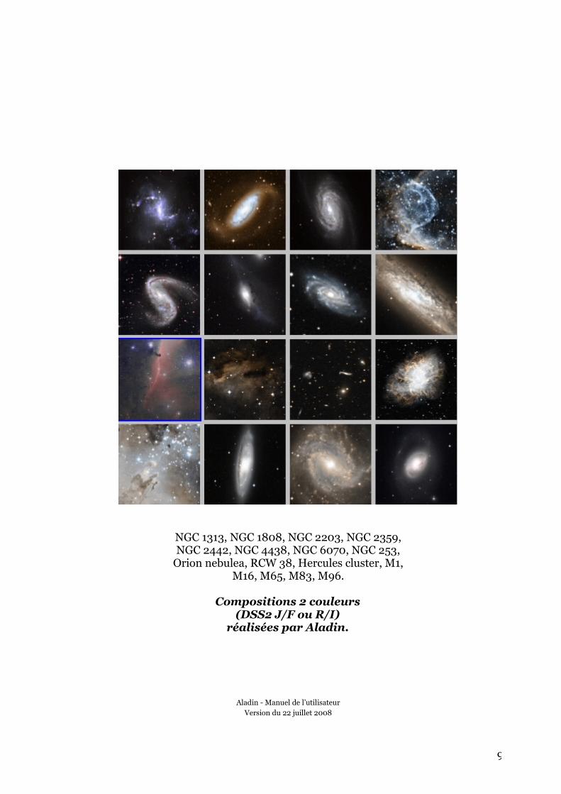
NGC 1313, NGC 1808, NGC 2203, NGC 2359,NGC 2442, NGC 4438, NGC 6070, NGC 253,

Orion nebulea, RCW 38, Hercules cluster, M1,M16, M65, M83, M96.

Compositions 2 couleurs(DSS2 J/F ou R/I)

réalisées par Aladin.

Aladin - Manuel de l’utilisateurVersion du 22 juillet 2008

9