air flow disturbance by moving objects at local exhaust

FACULTY OF ENGINEERING AND SUSTAINABLE DEVELOPMENT Department of Building, Energy and Environmental Engineering

Air flow disturbance by moving objects at local exhaust ventilation

Mikel Aguirre Sánchez

Jun 2015

Master’s Thesis, D Level, 15 ECTS Energy Systems

Master Programme in Energy Systems

Supervisor: Magnus Mattsson Examiner: Mathias Cehlin



Preface

I would like to express my deepest gratitude to my supervisor, Dr. Magnus Mattsson,

for his excellent guidance and dedication throughout this time. Not only for providing

useful information and advises, but also for sharing his vast knowledge with all the

difficulties encountered during this time.

I must acknowledge my colleague Leyre Catalán Ros for her support and effort, being

always available to lend a helping hand since I started the thesis. It has been a pleasure

working with her in the lab. Moreover, I would also like to thank Rickard Larsson, Hans

Lundström and Elisabet Linden for their assistance with all the technical issues arisen

during my stay in the lab.

Last but not least, I would like to thank my family for the unceasing encouragement,

support and attention.

My research would not have been possible without all of them.




Abstract

The present thesis aims to study the effect of human movements on local exhaust

ventilation.

In its simplest terms, local exhaust ventilation is a system which has the function of

extracting contaminated air situated close to the contaminant source, protecting a

working person from exposure to hazardous substances by containing or capturing them

locally, at the emission point. As an important security measure referred to terms of

health, it is crucial for the healthiness of workers to control and prevent them from the

exposure to vapour, mist, dust or other airborne contaminants. Additionally, to a lesser

degree of significance, it can be stressed an expected increase in worker performance

due to an improvement of the working conditions.

There is an existing necessity for well-defined and appropriate methods to test the

performance of local exhaust devices in order to reach standard efficiency values. The

lack of an international standardization led to the realization of this study, which,

ultimately, has the purpose of obtaining relevant results that can be utilized for future

normalized test procedures.

The study entails full scale experimental measurements that include air velocity

measurements in 3 dimensions, a local exhaust ventilation device with circular hood and

a flat flanged plate and a controlled generation of air turbulence through physical

movements of a human-sized cylinder, simulating a walking person.

The present study extends previous similar studies at the University of Gävle, where the

controlled air turbulence was generated by a moving plate. After meaningful results

obtained in that study, one of the considerations was to better simulate a walking

person, by replacing the plate for a movable cylinder. The present study points at a

larger similarity occurring with a cylinder than with a plate, as regards the air flow

pattern produced by a real walking person.

As in the previous study, the Percentage of Negative Velocities, PNV, has been used as

the main measure of turbulence induced risk of contaminant spread. The PNV

represents the fraction of the time when the flow is directed opposite to the suction air

stream in front of the local exhaust hood. The obtained results conclude that the use of

the cylinder as a moving object has been an improvement to simulate the effect of the

movement of a human being on a relaxed walking pace.



The present study was carried out in parallel with the thesis work by Leyre Catalán Ros

[17], which complements this study by analyzing the effect of an added heated dummy,

simulating a person seated in front of the local exhaust device.



Nomenclature

Cd Drag coefficient [-]

D Drag force experienced by an object due to the movement through a fully

enclosing fluid [N]

d Horizontal distance between the exhaust hood and the place of

measurements [mm]

EH Exhaust hood

h Vertical distance between the table and the place of measurements [mm]

L Reference length [m]

LEV Local exhaust ventilation

MC Movable cylinder

PNV Percentage of negative velocities [%]

Q Air flow rate in exhaust pipe [m3/s]

Re Reynolds number [-]

S Reference area [m2]

SA Sonic anemometer

U Air flow velocity [m/s]

u Air velocity in x axis direction [m/s]

V Flow velocity [m/s]

v Air velocity in y axis direction [m/s]

w Air velocity in z axis direction [m/s]

ΔP Pressure difference [Pa]

Δt Movement interval of the movable cylinder [s]

Viscosity coefficient [Pa.s]

ρ Air density [kg/m3]



1

Table of content

1. INTRODUCTION ....................................................................................................... 2

Local exhaust ventilation (LEV) ...................................................................................... 2

Literature review............................................................................................................... 3

Scope of the thesis ............................................................................................................ 5

2. THEORY ..................................................................................................................... 7

Interaction between fluid flow and a cylinder .................................................................. 7

Percentage of Negative Velocities .................................................................................. 11

3. METHOD .................................................................................................................. 12

Air velocity measurements ............................................................................................. 12

Calibration ...................................................................................................................... 13

The test room .................................................................................................................. 17

Exhaust device ................................................................................................................ 21

Positioning cases for the exhaust device ........................................................................ 22

Movable cylinder – turbulence generation ..................................................................... 23

4. RESULTS .................................................................................................................. 26

Comparison of air turbulence generated by the movable cylinder and a real walking

person ............................................................................................................................. 26

Percentage of Negative Velocities .................................................................................. 30

Air stabilization time ...................................................................................................... 31

Comparison of the PNV between the use of a movable cylinder and a movable plate .. 32

5. DISCUSSION ............................................................................................................ 34

6. CONCLUSIONS ....................................................................................................... 36

Reference ........................................................................................................................ 37

Appendices ..................................................................................................................... 39

Appendix A. Calibration of the 3-D sonic anemometer (SA) .................................... 39

Appendix B. Effect of the prongs ............................................................................... 41

Appendix C. Data filtration ........................................................................................ 43



2

1. INTRODUCTION

As it is known, the human exposure to a health harmful environment during a

prolonged period of time can lead to serious consequences. Therefore, when a

professional activity involves exposure to gases, dust or any other type of air

contaminant, it is essential to have a ventilation system that ensures the health of the

workers, avoiding unnecessary risks. Some of these potentially dangerous activities are,

for instance, when employees are exposed to high toxicity chemicals or when large

amounts of dusts or welding fumes are generated.

Local exhaust ventilation (LEV)

Local exhaust ventilation (LEV) is a system which has the function of extracting

contaminated air situated close to the contaminant source, protecting a working person

from exposure to hazardous substances by containing or capturing them locally, at the

emission point.

LEV operates on the principle that air moves from an area of high pressure to an area of

low pressure. The difference in low pressure is created by a fan that draws or sucks air

through the ventilation system. Local exhaust systems are located as close as possible to

the source of contamination to capture the contaminant before it is released into the

work area. [1] A local exhaust system has five basic elements as it can be seen in Fig. 1.

Figure 1. Elements of a local exhaust ventilation device [2].



3

1. An inlet/enclosure/hood: Where the contaminant is captured or contained and enters

the LEV.

2. Ducting: This conducts air and the contaminant from the hood to the discharge point.

3. Air cleaner or filter: This filters or cleans the extracted air. Not all systems need air

cleaning.

4. Air mover: The fan and motor that powers the extraction system.

5. Discharge or exhaust: This releases the extracted air to a safe place. [2]

Literature review

In a study performed by Mohd [3], different types of local exhaust ventilation were

monitored, proving the effectiveness of local exhaust ventilation in order to reduce

human exposure.

A previous study about the effect of local exhaust ventilation for the control of welding

fumes [4] indicates that LEV can reduce fume exposures to levels below currently

relevant standards. This same study suggests that 40–50% or more reduction in

exposure is possible with portable or fixed LEV systems relative to natural ventilation,

taking into account that correct positioning of the hood and adequate exhaust flow rates

are essential.

Another study that quantified the importance of LEV [5] assessed the effectiveness of a

commercially available LEV system for controlling respirable dust and crystalline silica

exposures during concrete grinding activities, concluding that the application of LEV

resulted in a reduction in the overall geometric mean respirable dust exposure from 4.5

to 0.14 mg/m3 , a mean exposure reduction of 92%.

According to a study about the exposure to volatile organic compounds in printing

plants [6], it was identified through computational fluid dynamics (CFD) analysis that

LEV was an effective mitigation measure. It was found that there existed a threshold

LEV air flow rate for an abrupt reduction in the worker’s exposure to volatile organic

compounds, noticing a less sensitive reduction when the LEV airflow was further

increased beyond the threshold; see in Fig. 2.



4

Figure 2. Susceptibility of worker to volatile organic compounds emissions versus push-pull LEV flow rate

according to computational fluid dynamics results. [6]

A study about the chemical exposure levels in hairdresser salons [7] dealt with the

significance of the usage of local exhaust ventilation in order to prevent from adverse

health effects related to their working environment. As it can be appreciated in Table 1,

exposure level values were considerably lower in the zones with LEV.

Table 1. Exposure level of ammonia in the breathing zone, measured in six hairdressing

salons. [7]

Additionally, in order to measure the effect on the local exhaust ventilation the

percentages of negative streamwise velocities for a determined period of time were

analysed in the present study. A similar case of study is described in the research

performed by Peter Lenaers and his colleagues about negative streamwise velocities

next to a wall for turbulent flows [8], showing relevant results.

In the present study a movable cylinder was used in order to simulate a walking person.

As a consequence of the movements of a person, the local air and the local contaminant

field may also change significantly, resulting in an increase of contaminant dispersion

as it is shown in the conclusions of the study performed by Welling [9].



5

The airflow field in indoor environment is normally characterized by high turbulent

level and unsteady flows. Generally, it is very difficult to conduct accurate and detailed

measurement of such a complex turbulent flow field with point-wise anemometry [10].

That complexity is added to the fact that in a workplace there are more variables to take

into account. When the contaminant removal effectiveness in a warmed room was

studied [11] it was demonstrated the importance of buoyancy forces for ventilation

effectiveness at low air change rates in a room heated by warm air. Furthermore, the

effect of increasing air change on the ventilation effectiveness was proved to be

dependent on the position of air terminal devices.

In the present study it has been used a flat flanged plate for the LEV hood. But it is

noteworthy that the addition of a flange to a local exhaust ventilation hood can produce

a large increase in velocity in front of the hood as it indicates a previous study about the

effect of flanges on the velocity in front of exhaust ventilation hoods [12]. In this study

the author concludes that as hood aspect ratio increases, the effect of flanges increases

and the addition of even small flanges to slots can have an appreciable effect.

To emphasize the importance of local exhaust ventilation a study analyzed the different

types of welding processes and exposures and the health hazards associated with

welding [13]. Welding is a common industrial process that generates a potentially

hazardous environment due to metal fumes and gases. According to this report most

long-time welders experience some type of respiratory disorder during their time of

employment.

Scope of the thesis

As previously mentioned, local exhaust ventilation is a system which has the function of

extracting contaminated air located close to the contaminant source, protecting a

working person from exposure to hazardous substances by capturing them at the

emission point.

There is an existing necessity for well-defined and appropriate methods to test the

performance of local exhaust devices in order to reach standard efficiency values. The

lack of international standardization methods led to the realization of this study, which,

ultimately, has the purpose of obtaining relevant results that can be utilized for future

normalized test procedures.

In his study [14], Mattsson proposed a method to test local exhaust ventilation systems.

The method mainly consisted in both air velocity measurements and tracer gas tests in a

controlled turbulence environment generated by the movement of a flat plate.

Nevertheless, as the turbulences generated by a flat plate were considerably higher to

those generated by a real human, the report suggested in its discussion that other shapes



6

should be tested as moving objects. Previously to the start of this thesis, it was held a

meeting between Swedish Work Environment Authority (SWEA), Swedish Standards

Institute (SIS) and three interested companies of local exhaust devices and Dr. Mattsson

in representation of the University of Gävle. In that meeting all the parts reached to the

agreement that it was considered of interest the study of the usage of a cylinder as

movable object, since a cylinder has a more similar aerodynamic behaviour to the

human-being one.

Thus, the main objective of this research study is to test and analyze the effect generated

by a moving cylindrical shape on local exhaust ventilation, in order to obtain relevant

results to contribute to the establishment of standardization in local exhaust ventilation

testing.

For this purpose the study entails full scale experimental measurements that include air

velocity measurements in 3 dimensions, a local exhaust ventilation device with circular

hood and a flat flanged plate and a controlled generation of air turbulence through

physical movements of a human-sized cylindrical shape simulating a walking person.

In order to analyze the results obtained, the Percentage of Negative Velocities, PNV,

have been used as the main measure of turbulence induced risk of contaminant spread.

The PNV represents the fraction of the time measured when the velocity of the flow for

a given direction moves on the opposite way to the air stream. It was previously found

by Mattsson [14] that PNV correlates well with LEV capture efficiency, as quantified

with tracer gas.

In the present study the results of the usage of a movable cylinder and the movement of

a real person are compared, with the intention to investigate the similarity between the

effect of the movement of a cylindrical shape and the one of a real walking person.



7

2. THEORY

In this section some important concepts are theoretically described for a better

understanding of the research study. Two main topics regarding the air flow effect when

it interacts with a cylinder and the Percentage of Negative Velocities are below defined.

Interaction between fluid flow and a cylinder

The movement of a fluid can be classified in many ways, according to different criteria

and according to its different characteristics. For the comprehension there are some

terms that should be previously explained, like the aerodynamic drag. [15]

In aerodynamics, aerodynamic drag is the fluid drag force that acts on any moving solid

body in the direction of the fluid freestream flow. From the body's perspective, the drag

comes from forces due to pressure distributions over the body surface and forces due to

skin friction, which is a result of viscosity.

The aerodynamic drag on an object depends on several factors, including

the shape, size, inclination and flow conditions. All of these factors are related to the

value of the drag through the drag equation. The drag equation is a formula used to

calculate the force of drag experienced by an object due to movement through a fully

enclosing fluid. The drag equation is defined as

D =

Cd ρ S V

2

where,

D is equal to the drag force [N]

Cd is the drag coefficient [-]

ρ is the air density [kg/m3]

S is the reference area [m2]

and V is the flow velocity [m/s].

The drag coefficient is a dimensionless number that characterizes all of the complex

factors that affect drag. The drag coefficient in air is usually

determined experimentally using a model in a wind tunnel. In the tunnel, the velocity,

density, and size of the model are known. Measuring the drag then determines the value

of the drag coefficient as given by the above equation. The drag coefficient and the drag

equation can then be used to determine the drag on a similar shaped object at different

flow conditions as long as several flow similarity parameters are matched. In

particular, Mach number similarity insures that the compressibility effects are correctly

http://en.wikipedia.org/wiki/Aerodynamics

https://www.grc.nasa.gov/www/K-12/airplane/shaped.html

https://www.grc.nasa.gov/www/K-12/airplane/sized.html

https://www.grc.nasa.gov/www/K-12/airplane/airsim.html

https://www.grc.nasa.gov/www/K-12/airplane/drageq.html

http://en.wikipedia.org/wiki/Drag_(physics)

http://en.wikipedia.org/wiki/Fluid

https://www.grc.nasa.gov/www/K-12/airplane/tunnel1.html



8

modelled, and Reynolds number similarity ensures that the viscous effects are correctly

modelled. The Reynolds number is the ratio of the inertia forces to the viscous forces

and is given by:

Re = V ρ

where,

V is the flow velocity [m/s]

ρ is the air density [kg/m3]

l is the reference length [m]

and is the viscosity coefficient [Pa.s].

For most aerodynamic objects, the drag coefficient has a nearly constant value across a

large range of Reynolds numbers. But for a simple cylindrical shape, the value of the

drag coefficient varies widely with Reynolds number as shown in Fig. 3.

Figure 3. Drag coefficient as a function of Reynolds number for long circular cylinders. [16]

To understand these variations, some different cases at the flow past a cylinder are

going to be explained. Flow past a cylinder goes through a number of transitions with

velocity it can be observed in Fig. 5, 6, 7, 8 and 9. Five different cases have been

selected. These theoretical cases are considered to maintain the same density and

viscosity of the fluid flow, as well as the same diameter of the cylindrical shape. The

flow has been gradually increased to increase the Reynolds number. The drag for each

case number is noted on the Fig. 4.



9

Figure 4. Drag coefficient for each studied case numbered on from 2 to 5. [15]

Case 1. Ideal – Flow Attached

Case 1 shows very slow flow in which viscosity has been entirely neglected. There is

an ideal flow with no boundary layer along the surface, completely attached flow (no

separation) and no viscous wake downstream of the cylinder. Due to the flow is

symmetric from upstream to downstream, there is no drag on the cylinder. This strange

result is called d'Alembert's paradox, after the early mathematician who studied the

problem. Neglecting viscosity simplifies the analysis, but this type of flow does not

occur in nature where there is always some small amount of viscosity present in any

fluid.

Case 2. Separated – Steady

Figure 6. Case 2. Separated – Steady. [15]

Figure 5. Case 1. Ideal – Flow Attached. [15]



10

Case 2 illustrates what occurs for low velocity flows. Two stable vortices are formed on

the downwind side of the cylinder. The flow is separated but steady and the vortices

generate a high drag on the cylinder.

Case 3. Unsteady - Oscillating

Figure 7. Case 3. Unsteady – Oscillating. [15]

Case 3 shows the flow as velocity is increased. The downstream vortices become

unstable, separate from the body and are alternately shed downstream. The wake is very

wide and generates a large amount of drag. The alternate shedding is called the Karman

vortex street. This type of flow is periodic; it is unsteady but repeats itself at some time

interval. The pressure variation associated with the velocity changes produces

a sound called an aeolian tone. This is the sound can be heard for instance when the

wind blows over high-power wires. It is a low frequency (low pitch), haunting tone.

Case 4. Laminar - Separated

Figure 8. Case 4. Laminar – Separated. [15]

Case 4 shows the flow as the velocity is increased even more. The periodic flow breaks

down into a chaotic wake. The flow in the boundary layer on the windward side of the

cylinder is laminar and orderly and the chaotic wake is initiated as the flow turns onto

the leeward side of the cylinder. The wake is not quite as wide as for Case 3, so the drag

is slightly less.



11

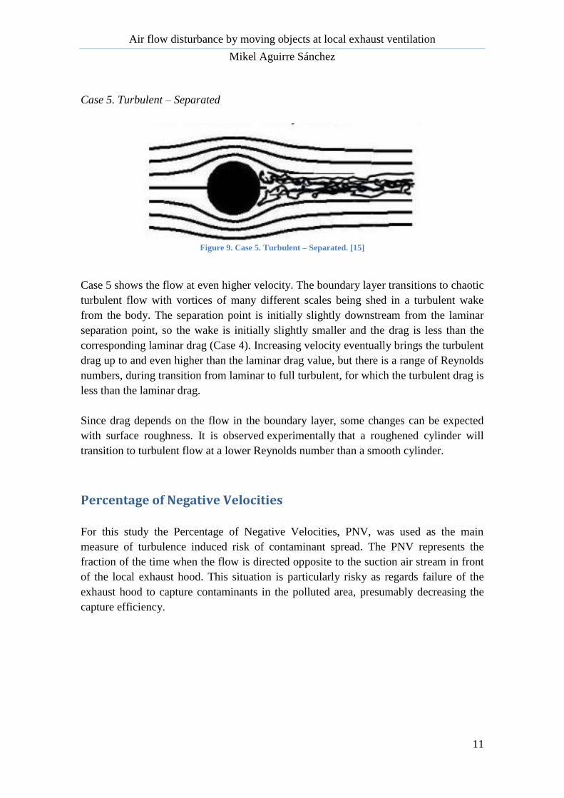
Case 5. Turbulent – Separated

Figure 9. Case 5. Turbulent – Separated. [15]

Case 5 shows the flow at even higher velocity. The boundary layer transitions to chaotic

turbulent flow with vortices of many different scales being shed in a turbulent wake

from the body. The separation point is initially slightly downstream from the laminar

separation point, so the wake is initially slightly smaller and the drag is less than the

corresponding laminar drag (Case 4). Increasing velocity eventually brings the turbulent

drag up to and even higher than the laminar drag value, but there is a range of Reynolds

numbers, during transition from laminar to full turbulent, for which the turbulent drag is

less than the laminar drag.

Since drag depends on the flow in the boundary layer, some changes can be expected

with surface roughness. It is observed experimentally that a roughened cylinder will

transition to turbulent flow at a lower Reynolds number than a smooth cylinder.

Percentage of Negative Velocities

For this study the Percentage of Negative Velocities, PNV, was used as the main

measure of turbulence induced risk of contaminant spread. The PNV represents the

fraction of the time when the flow is directed opposite to the suction air stream in front

of the local exhaust hood. This situation is particularly risky as regards failure of the

exhaust hood to capture contaminants in the polluted area, presumably decreasing the

capture efficiency.



12

3. METHOD

Air velocity measurements

The air velocity was measured by using a set of Kaijo Ultrasonic Anemometer DA-650

(SA) with TR-92T probes; see in Fig. 10. The TR-92T anemometer probes had a 30 mm

span size. The small span size minimizes the measurement error caused by volume

averaging. The probes of the SA were placed at the end of each prong, containing a total

of six prongs, three long and three short, interspersed with each other. The DA-650

Ultrasonic Anemometer sampled the air velocity in x-, y-, and z-directions at 20 Hz

frequency. The resolution of the SA was 0.005 m/s. The SA was also able to measure

air temperature, but regular calibration is needed.

Figure 10. 3-D Sonic Anemometer, SA, in front of the exhaust hood, EH.

The length of the measuring volume in the direction of the expected main air flow was

12 mm. The SA was always oriented such that the expected main air flow direction –

towards the exhaust nozzle centre – implied that no prongs were situated “upstream”,

since they then partly would obstruct the measuring volume. This optimum orientation

was determined to be the one with the x axis directed to the exhaust nozzle centre as it is

shown in Fig. 11 and Appendix B.



13

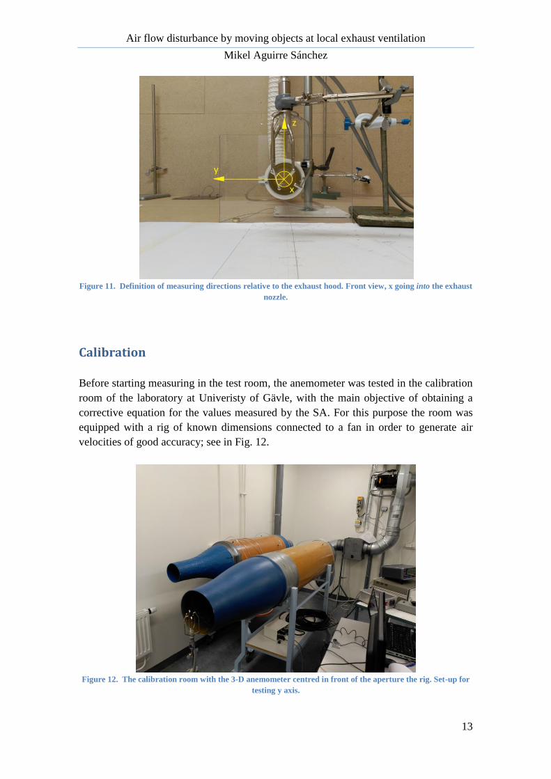
Figure 11. Definition of measuring directions relative to the exhaust hood. Front view, x going into the exhaust

nozzle.

Calibration

Before starting measuring in the test room, the anemometer was tested in the calibration

room of the laboratory at Univeristy of Gävle, with the main objective of obtaining a

corrective equation for the values measured by the SA. For this purpose the room was

equipped with a rig of known dimensions connected to a fan in order to generate air

velocities of good accuracy; see in Fig. 12.

Figure 12. The calibration room with the 3-D anemometer centred in front of the aperture the rig. Set-up for

testing y axis.



14

The air flow ejected from the aperture of the rig was measured by using a PPC500

Pressure Calibrator shown in Fig 13. The PPC500 was calibrated against Furness

Controls’ FRS4 Primary Pressure Standards, having a 0.01% uncertainty with an

ultimate resolution at 0.01 Pa. The possibility to regulate the air pressure by using a

controller enabled to test different known pressure differences.

Figure 13. PPC500 Pressure Calibrator.

As the air speed as measured with a sonic anemometer varies with temperature, before

starting doing the measurements the temperature sensor integrated in the SA was set

with the temperature measured in the same moment by a more precise temperature

sensor, the Systemteknik AB S1220 series shown in Fig. 14.

Figure 14. Systemteknik AB S1220 Series temperature sensor measuring the temperature of the room.



15

When calibrating the SA, it was placed in front of the aperture of the rig, centred, as

close as possible. To analyze the flow along each axis of the anemometer, the position

of the SA was varied such that the axis to study was placed perpendicularly to the

aperture of the rig; see in Fig. 15.

Figure 15. Air flow velocity calibration test, y axis case.

Additionally, for obtaining the mathematical value of the air velocity in the aperture of

the rig the next equation was used, which is referred to the calibration curve for the

given rig; see in Fig. 16.

Where U is the air flow velocity and is the pressure difference in the rig.

Figure 16. Calibration curve of the rig.



16

The pressure differences assessed relevant for the study were between 0 Pa and 100 Pa,

corresponding to 0 m/s and 1.5 m/s respectively. Each test lasted 2 minutes. By

analyzing about 16 different air velocities for each axis, both measured values and

mathematically obtained values were compared. From this, a correction equation was

obtained for the air velocity of each axis. The diagrams of the obtained results are

shown in Appendix A.

Since the sonic anemometer produced a noise signal of random fluctuations within

about ±0.02 m/s, which was considered influential on some of the data analysis, the raw

air velocity data were after-filtered using the Matlab (MathWorks, Inc.) function “filter”

set as low pass filter with a time constant of 0.2 s; see in Appendix C. The measuring

uncertainty of the sonic anemometer, after data filtration and applying direction

corrections, was estimated at ±10%.

To reduce the air movements in the calibration room and obtain more accurate data, the

ventilation system of the room was blocked in order to avoid possible air flows which

could affect the test. In the same way, a panel was placed between researchers and test

area to act as a barrier in order to reduce variations in the air due to the movements and

breathing researchers; see in Fig. 17.

Figure 17. Panel between the seats of the researchers and the anemometer. SA testing z direction.

For each test the same measures were taken into account to verify the accuracy of the

tests. During measurements, silence was kept in the room and also no movement was

performed. Before each test, it was waited a time of one minute without making any



17

movement or noise to stabilize the air. In the case that the door of the calibration room

had been opened, a prudential time of 3 minutes was maintained to stabilize the air in

the room.

The test room

To perform the relevant trials a test room placed in the building number 45 of the

University of Gävle was used. The test room, shown in the Fig. 18, was one of the three

rooms in the test building situated in the lab hall; Fig 19. It was the same room as used

by Mattsson in his research [13], in order to do a comparative analysis. A drawing of

the test room and its surroundings is shown in Fig. 20. The ceiling height in the test

room was 3.00 m and its room volume was 54.7 m3. The building envelope of the test

building, including inner walls, consisted mainly of wooden boards with 5-10 cm

mineral wool insulation in between. The temperature of test room was maintained at

about 22 ºC, with a variation of 2ºC due to the heat stemming from lighting, measuring

equipment and body heat of the researchers. Except ceiling lighting and measuring

equipment there was no heating in the test building.

Figure 18. Test room with the local exhaust and movable cylinder arrangement. Set up for test Case B, 2D.



18

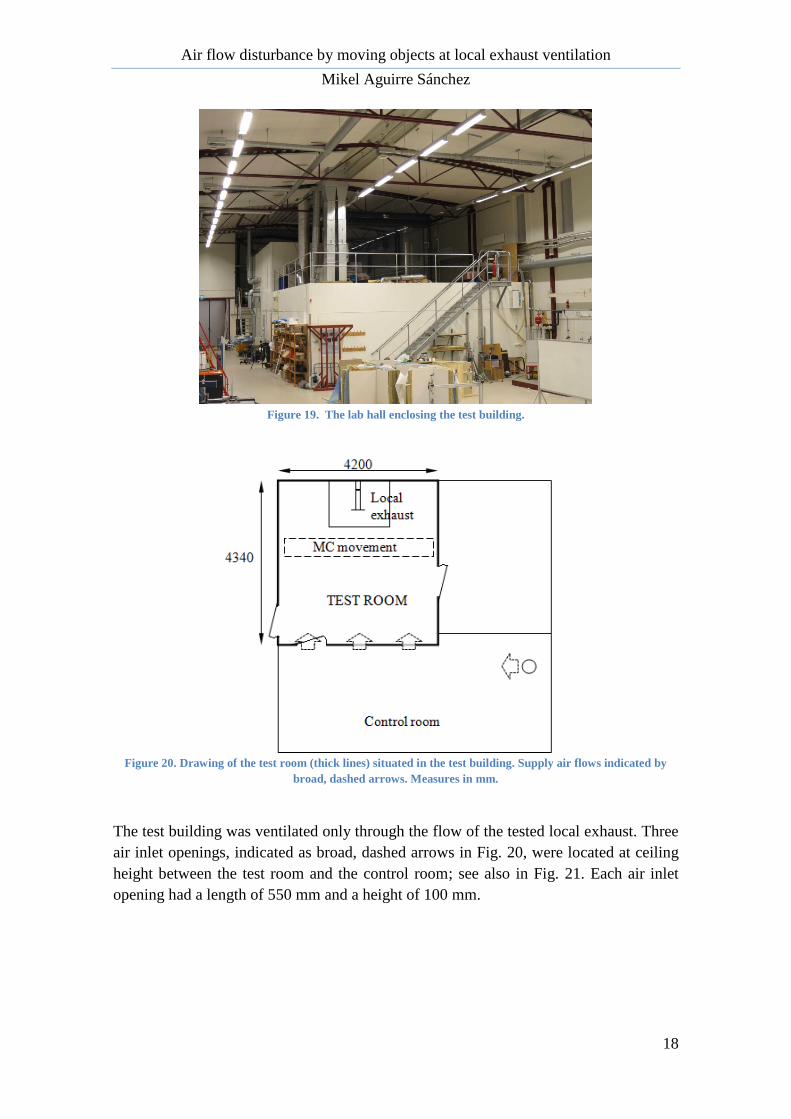
Figure 19. The lab hall enclosing the test building.

Figure 20. Drawing of the test room (thick lines) situated in the test building. Supply air flows indicated by

broad, dashed arrows. Measures in mm.

The test building was ventilated only through the flow of the tested local exhaust. Three

air inlet openings, indicated as broad, dashed arrows in Fig. 20, were located at ceiling

height between the test room and the control room; see also in Fig. 21. Each air inlet

opening had a length of 550 mm and a height of 100 mm.



19

Figure 21. Three air inlets at the top of the wall viewed from control room.

Furthermore, on the test room side, a 500 mm high plate, extending across the whole

width of the room wall, deflected the incoming air downwards, as illustrated in Fig. 22

and Fig. 23. This arrangement intended to produce an inlet air flow that caused very

little air turbulence in the test room, especially in the area around the local exhaust.

Figure 22. Supply air deflecting plate at the top of the test room wall.

Additionally, the air of the control room was aspirated from the lab hall through a

130 mm diameter hole in the ceiling. Some air was likely to have entered the test room

also through minor leaks, e.g. at the doorways, none of which were close the local

exhaust installation. All doors were closed during the tests. Prior to the start of each

measurement it was remained a precautionary time so that the air inside the test room

had stabilized.



20

Figure 23. Side-view of the air inlet to the test room. Measures in mm. Slot width 100 mm.

The exhaust air flow through the exhaust hood, EH, was regulated through the speed of

a fan placed outside of the test room; see in Fig. 24, eventually discharging the exhaust

air to outdoors.

The exhaust air flow rate, Q, was measured through the pressure drop over an orifice

plate (Standard ISO 5167:2003) of diameter 68.5 mm in a straight duct of diameter

104 mm; see in Fig 24. The pressure drop was measured with a newly calibrated

differential pressure gauge (SwemaMan 80, Swema AB, Farsta, Sweden), yielding a

total uncertainty of the flow rate of about 2%.

Figure 24. Test room roof. Fan for exhaust ventilation and pressure drop orifice plate.



21

Exhaust device

For the tests performed it was used a local exhaust ventilation (LEV) device as the main

component for extracting the supposed contaminated air of the room. The LEV device

consisted of a 400 mm long straight aluminium cylinder with an inner diameter of

75 mm, connected to the exhaust fan of the roof through a tube of the same diameter.

The exhaust inlet opening was equipped with a 300 mm wide and 200 mm high flat

plate, centred onto the inlet, thus forming a simple, exterior, flanged exhaust hood (EH).

The EH was placed on a wooden table whose dimensions were 900 mm high, 1640 mm

wide and 1220 mm deep; see in Fig. 25.

Figure 25. EH over the table, placed behind the SA. Positioning for Case A, d=3D.

The different exhaust air flow rates, Q, used in the tests and the corresponding pressure

difference across orifice plate and the target pressure in the exhaust hood are listed in

Table 2.

Table 2. Exhaust air flow related to target pressure.

Exhaust air flow

rate, Q [ m3/h ]

Pressure difference

across orifice plate

[ Pa ]

Correction [Pa] Target pressure [ Pa ]

50 17.2 +0.2 17.0

100 71.8 -0.15 72.0

150 164 +0.4 163.5



22

Positioning cases for the exhaust device

According to the agreement reached by the University of Gävle, Swedish Standards

Institue (SIS), Swedish Work Environment Authority (SWEA) and three interested

manufacturers of local exhaust devices, some specific positions were considered to be

tested.

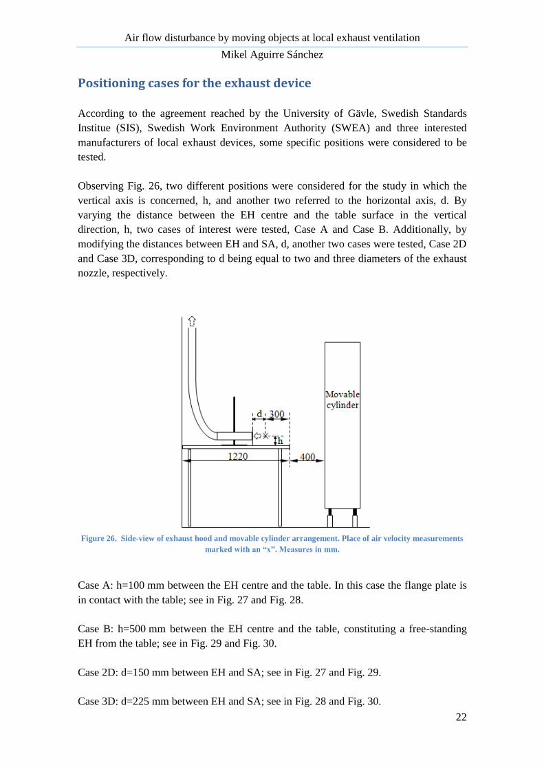
Observing Fig. 26, two different positions were considered for the study in which the

vertical axis is concerned, h, and another two referred to the horizontal axis, d. By

varying the distance between the EH centre and the table surface in the vertical

direction, h, two cases of interest were tested, Case A and Case B. Additionally, by

modifying the distances between EH and SA, d, another two cases were tested, Case 2D

and Case 3D, corresponding to d being equal to two and three diameters of the exhaust

nozzle, respectively.

Figure 26. Side-view of exhaust hood and movable cylinder arrangement. Place of air velocity measurements

marked with an “x”. Measures in mm.

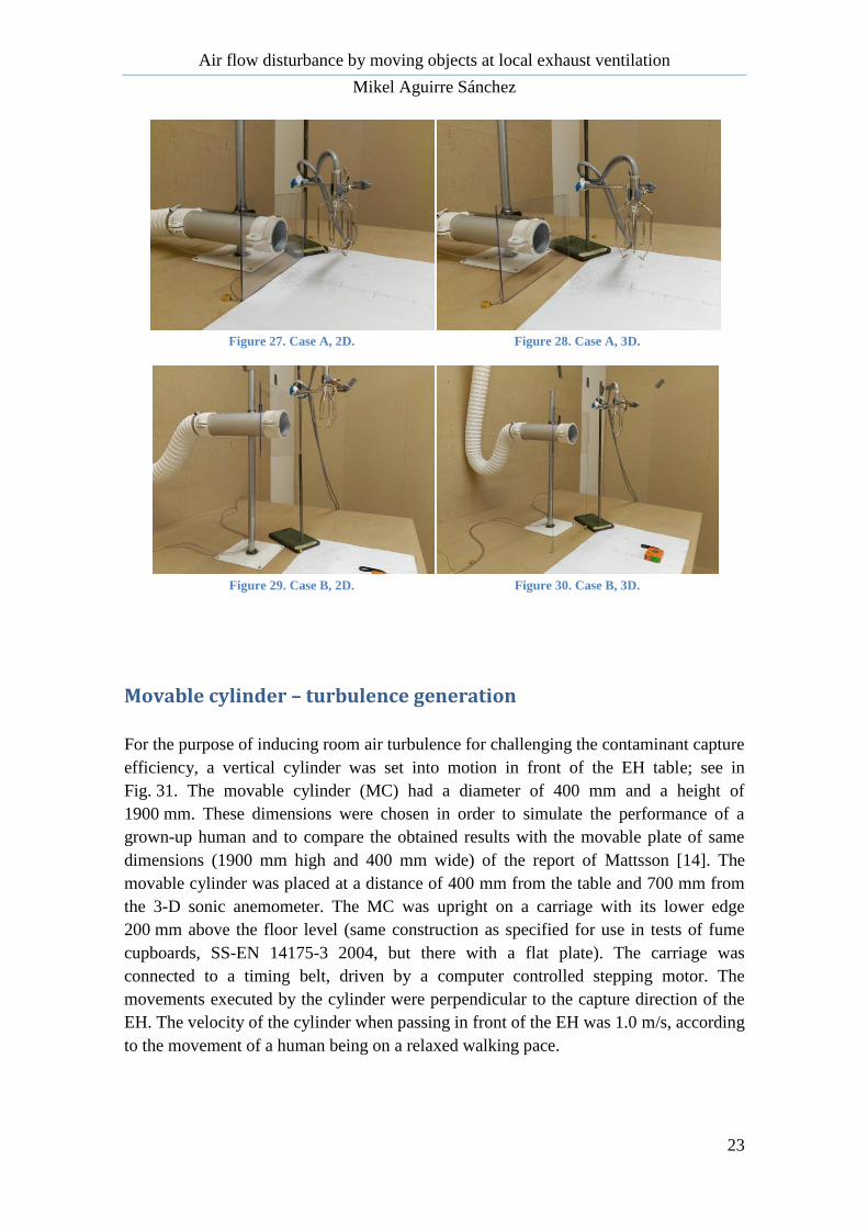
Case A: h=100 mm between the EH centre and the table. In this case the flange plate is

in contact with the table; see in Fig. 27 and Fig. 28.

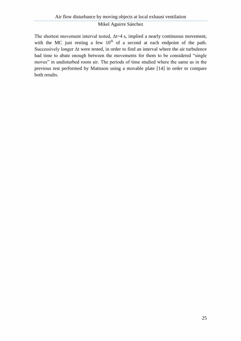
Case B: h=500 mm between the EH centre and the table, constituting a free-standing

EH from the table; see in Fig. 29 and Fig. 30.

Case 2D: d=150 mm between EH and SA; see in Fig. 27 and Fig. 29.

Case 3D: d=225 mm between EH and SA; see in Fig. 28 and Fig. 30.



23

Figure 27. Case A, 2D. Figure 28. Case A, 3D.

Figure 29. Case B, 2D. Figure 30. Case B, 3D.

Movable cylinder – turbulence generation

For the purpose of inducing room air turbulence for challenging the contaminant capture

efficiency, a vertical cylinder was set into motion in front of the EH table; see in

Fig. 31. The movable cylinder (MC) had a diameter of 400 mm and a height of

1900 mm. These dimensions were chosen in order to simulate the performance of a

grown-up human and to compare the obtained results with the movable plate of same

dimensions (1900 mm high and 400 mm wide) of the report of Mattsson [14]. The

movable cylinder was placed at a distance of 400 mm from the table and 700 mm from

the 3-D sonic anemometer. The MC was upright on a carriage with its lower edge

200 mm above the floor level (same construction as specified for use in tests of fume

cupboards, SS-EN 14175-3 2004, but there with a flat plate). The carriage was

connected to a timing belt, driven by a computer controlled stepping motor. The

movements executed by the cylinder were perpendicular to the capture direction of the

EH. The velocity of the cylinder when passing in front of the EH was 1.0 m/s, according

to the movement of a human being on a relaxed walking pace.



24

Figure 31. Local exhaust and movable cylinder arrangement.

At an initial stage, the span of the MC movement was 2770 mm, centrally positioned

between the two side walls. The acceleration and retardation of the MC was 1.4 m/s2,

resulting in the sustained speed of 1.0 m/s prevailing over almost 1770 mm distance,

preceded by a 500 mm acceleration distance and ended by a 500 mm retardation

distance. After testing every 2D cases, and due to some technical issues, the parameters

of the MC movement were changed to 2900 mm of span (starting point at 100mm and

ending point at 3000 mm of the carriage) and 2.0 m/s2 of acceleration and retardation,

but maintaining the sustained speed of 1.0 m/s prevailing over the relevant area. The

variations of these parameters had no notable effect in the tests.

At each test with the MC in action, it was programmed to make repeated traversing

moves like this at a steady movement interval, Δt. The intervals tested are listed in

Table 3 below. A “movement” here means one passage across the room, being either to

the right or to the left.

Table 3. Movement intervals of the movable cylinder.

Nominal movement

interval, Δt [ s ]

Actual movement

interval [ s ]

Movement frequency

[ min-1

]

4 4.4 14 (Continuous movements)

10 10.4 6

30 30.6 2

60 60.8 1



25

The shortest movement interval tested, Δt=4 s, implied a nearly continuous movement,

with the MC just resting a few 10th

of a second at each endpoint of the path.

Successively longer Δt were tested, in order to find an interval where the air turbulence

had time to abate enough between the movements for them to be considered “single

moves” in undisturbed room air. The periods of time studied where the same as in the

previous test performed by Mattsson using a movable plate [14] in order to compare

both results.



26

4. RESULTS

Comparison of air turbulence generated by the movable cylinder

and a real walking person

To quantify the effect of the disturbances generated by the movable cylinder (MC)

through the measurements of the SA, the MC was set into regular motion at the

different time intervals, t, previously listed in Table 3, with a fixed duration according

to Table 4 below.

Table 4. Movement intervals and time of action for the movable cylinder, MC.

Nominal movement

interval, Δt [ s ]

Time of action

[ min ]

4 6

10 7

30 8

60 10

The results of the movable cylinder MC obtained in the present study are compared to

the ones obtained in the study of Mattsson [14] for a movable plate and also for a real

walking person. Note that to be able to compare the results of the three different tests it

must be selected an identical case.

Thus, for a given case, Case A 2D (Δt=60 s Q=100 m3/h), three different results for the

u velocity, referred to x axis direction (towards the EH), are shown in Fig. 32, Fig. 33

and Fig. 34. The results correspond to the MC case, the movable plate case and the real

person case respectively.



27

Figure 32. Air velocity u, x axis direction. MC movements at Δt=60 s. Q=100 m3/h. Case A, 2D.

Figure 33. Air velocity u, x axis direction. Movable plate movements at Δt=60 s. Q=100 m3/h. Case A, 2D (from

[14]).

Figure 34. Air velocity u, x axis direction. Effect of a real walking person at Δt=60 s. Q=100 m3/h. Case A, 2D

(from [14]).

-0.05

0.00

0.05

0.10

0.15

0.20

0.25

0.30

0.35

0 1 2 3 4 5 6 7 8 9 10 11 12 13 14

Air

ve

loci

ty,

Vx

[ m

/s ]

Time [ min ]

-0.05

0.00

0.05

0.10

0.15

0.20

0.25

0.30

0.35

0 1 2 3 4 5 6 7 8 9 10 11 12 13 14

Air

ve

loci

ty,

Vx

[ m

/s ]

Time [ min ]



28

As it can be appreciated, the three cases draw a similar shape. Nevertheless, the

movable plate shows higher peaks of velocity than the order cases when the turbulences

are generated. In the case of the movable cylinder, the peaks have a similar shape to the

ones of the real person, but the turbulence is slightly lower in the MC case.

In the following diagrams shown in Fig. 35, Fig. 36 and Fig. 37 the three velocities, u, v

and w referred to x, y and z axis resp., are represented for the same cases; movable

cylinder, movable plate and a walking real person respectively.

Figure 35. Air velocities u, v and w. MC movements at Δt =60 s. Q =100 m3/h. Case A, 2D.

Figure 36. Air velocities u, v and w. Movable plate movements at Δt =60 s. Q =100 m3/h. Case A, 2D (from

[14]).

-0.35

-0.25

-0.15

-0.05

0.05

0.15

0.25

0.35

6.7 7.2 7.7 8.2 8.7

Air

ve

loci

tie

s [m

/s]

Time [min]

u

v

w

-0.35

-0.25

-0.15

-0.05

0.05

0.15

0.25

0.35

6.7 6.8 6.9 7.0 7.1 7.2 7.3 7.4 7.5 7.6 7.7 7.8 7.9 8.0 8.1 8.2 8.3 8.4 8.5 8.6 8.7

Air

ve

loci

tie

s [

m/s

]

Time [ min ]

Vx

Vy

Vz



29

Figure 37. Air velocities u, v and w. Effect of a real walking person at Δt =60 s. Q =100 m3/h. Case A, 2D (from

[14]).

The diagrams show how the movable plate case implies larger peaks than other cases,

sharing more fluctuation and peak values the movable cylinder case and the real

walking person. However, the movable cylinder case maintains a slightly lower level of

turbulence in all the three directions.

Before the initial movement, when the air in the test room was stabilized, at the quite

low air turbulence level it could be said that the air in the room was moving nearly

straight in the direction to the EH as a laminar flow. When the moving shape made a

movement, it generated a peak in the velocity axis due to a horizontal vortex around the

SA. Afterwards, the vortex was dissolved and u, v and w velocities gradually recovered

their initial velocities. It can be also appreciated that during the turbulent regime, just

after the movement of the moving device, some of the velocity values were negative,

moving the air in the opposite way of desired in case of u velocity and escaping from

the EH zone. Air velocity negative values can be clearly observed in Fig. 38, which is

referred to the diagram of Case A-3D, movement interval of 4 s and air flow velocity of

50 m3/h, with a PNV of 41%.

Figure 38. Air velocity u, x axis direction. MC movements at Δt=4 s. Q=50 m3/h. Case A, 3D. PNV=41%.

-0.35

-0.25

-0.15

-0.05

0.05

0.15

0.25

0.35

6.7 6.8 6.9 7.0 7.1 7.2 7.3 7.4 7.5 7.6 7.7 7.8 7.9 8.0 8.1 8.2 8.3 8.4 8.5 8.6 8.7

Air

ve

loci

tie

s[

m/s

]

Time [ min ]

Vx

Vy

Vz



30

Percentage of Negative Velocities

Above was observed that the movement of the movable cylinder occasionally generates

negative velocities in the direction of x axis, u velocity, which represents an opposite

effect to the desired one. Thus the extraction efficiency of the exhaust system can be

expected to be reduced, with the consequent risk of polluting the air of the working

area.

The Percentage of Negatives Velocities, PNV, is the measure that represents the

percentage of the time when the air flow has the opposite direction to the exhaust flow

along the x axis. The studied periods of time are shown in the Table 4, which represent

not only the time spent by the MC to go from one side to the other, but also the resting

period between the movement intervals.

To summarize the results of the recorded PNV values, the diagrams for the different

cases have been compiled in order to make the results comparable; see in Fig. 39.

Figure 39. Percentage of Negative Velocities, PNV, at the different test cases, movement intervals, Δt, and

exhaust flow rates, Q.

As it can be seen in Fig. 39, the diagrams show some general tendencies to take into

consideration. (1) At lower exhaust flow rates, Q, the PNV value increases. (2) By

increasing the distance between the exhaust hood, EH, and the testing point where the

3-D sonic anemometer, SA, was placed, the PNV values experience a rise. (3) When the

exhaust hood, EH, is placed at a larger distance from the supporting surface, in this case

the table, the PNV value increases. (4) By reducing the movement interval time, Δt, the

PNV value gets higher. Note that some values do not follow this last trend at low




31

Air stabilization time

Some measures were repeated due to results that were outside the logical range of

values; see in Fig. 40. Those cases were concretely the ones for 3D distance between

EH and SA, for an exhaust air flow rate, Q, of 50 m3/h.

Figure 40. Comparison between initial measure, Wrong, and repeated measure, Correct, for a 3D distance for

cases A and B. Measured in Percentage of Negative Velocities, PNV, at different movement intervals, Δt, and


It was considered to repeat the same procedure as in the other tests. Nevertheless, when

those cases were repeated it was waited a prudential time of 3 minutes before each test

in order to stabilize the air in the test room. As it can be seen in Fig. 40, the differences

in the values are remarkable, especially in Case A, Q=50 m3/h, Δt=4 s.



32

Comparison of the PNV between the use of a movable cylinder and

a movable plate

One of the main objectives of this study was to see how a movable cylinder affects the

exhaust capture efficiency as compared to the previous study performed by Mattsson

[14], where instead a movable plate was used to simulate the movement of a walking

person. For this purpose the cases studied by Mattsson were reproduced in order to

make the results comparable, modifying only the moving object, see in Fig. 41.

Figure 41. Comparison between using a movable plate (left) [14] and a movable cylinder (right).

In Fig. 42 is shown a comparison between the recorded PNV values for the studied

cases using a movable cylinder and the same cases using a movable plate. The results of

the movable plate PNV were directly obtained from the report of Mattsson [14].

For a clearer understanding of the results, the PNV values due to the movement of the

movable cylinder cases are placed on the left column, whereas the PNV values when

using the movable plate are the ones on the right column, maintaining the same order to

facilitate the comprehension of the results.



33

Movable Cylinder Cases Movable Plate Cases

Figure 42. Comparison of PNV values between using the movable cylinder, MC (left), and using a movable

plate [14] (right). Note that the scale on the PNV axis for Case B_3D is higher than the rest.

As it is visible in Fig. 42, the general trend is that (1) PNV values for the cases that use

the movable cylinder, MC, in general are lower compared to the movable plate,

although a few exceptions exist. Especially when the exhaust air flow rate is increased

the PNV values for the MC cases are clearly lower, probably due to other aerodynamics

produced by the moving device. Furthermore, (2) it is especially for the shorter distance

between the exhaust hood and the 3-D sonic anemometer, concretely 2D cases, that the

PNV values are considerably lower in MC cases.



34

5. DISCUSSION

The present study has verified that PNV may be considered a relevant measure of local

exhaust performance. The fact that obtained changes in PNV at different test cases have

corresponded roughly to the expected ones enhances the veracity and credibility of PNV

as a useful quantity.

As has been previously explained, this study was preceded by one performed by

Mattsson [14] in which the effect of the turbulence generated by a moving plate on a

local exhaust ventilation device was studied. At the end of that study the possibility of a

new research by modifying the moving plate used for another shape was suggested. For

this reason a movable cylinder was constructed imitating the dimensions of the moving

plate, both in turn imitating the body of an adult human being. The purpose was to

obtain results that simulate the effects of a real person with greater fidelity. Hence, to

provide this research with the greatest trustworthiness, the conditions of the study

performed Mattsson [14] have been reproduced in order to develop the tests in a

repeatable manner. Therefore, it has been possible to compare the obtained results and

to conclude that the use of the cylinder as moving object has been an improvement and

a correct approach to simulate the effect of the movement of a human being on a relaxed

walking pace.

Compared to moving plate and real human walking results [14], the turbulence pattern

generated by the moving cylinder are in line with the supposed results. As expected, the

moving cylinder generated considerably less turbulence than that of the moving plate,

probably due to a difference in the produced aerodynamics. On the other hand, the

movable cylinder produced similar turbulence that the generated by the real walking

person, considering slightly less turbulence for the movable cylinder case, although as it

is explained [14] the tested person was gently swinging the arms, which ought to

enhance turbulence. Even though the cylinder has had satisfactory results, it could be

considered some improvements that simulate the behaviour of human body closer.

Some of these factors to consider could be the breathing of a relaxed person, the body

heat or the movement generated when swinging arms and legs.

In practise, a person would not only walk perpendicularly to the exhaust air flow

direction. Hence, it could be interesting to analyze the effect of the moving object in

different directions to the one performed in this study to observe the variations in the

results. Other measures than PNV of the occurring turbulence might also be appropriate

to include in future studies.



35

Concerning the limitations, it should be considered that due to some technical issues,

the span of the movement of the cylinder was not maintained always centred and in

some tests had less acceleration. All the same, the velocity of the cylinder when passing

next to the exhaust hood was always 1.0 m/s, with no appreciable variations.

By using a 3-D sonic anemometer (SA) it has been possible to sample the movement of

the air flow in a very precise way. Nevertheless some problems were found when using

this measuring device. The prongs that hold the probes interact with the airflow under

study, thereby reducing its accuracy. Although it was tried to correct this error by

calibrating the SA and creating corrective equations, thus obtaining better accuracy, it

would be interesting to find out a solution to minimize this measuring error.

Additionally, as a complement to the present study, Leyre Catalán Ros [17] carried out

tracer gas measurements to analyze the capture efficiency of the local exhaust

ventilation, including the presence of a heated dummy, simulating a person in his

workplace exposed to a contaminant. This study also involved exposure measurements

in the breathing zone.



36

6. CONCLUSIONS

The main conclusion that can be drawn is that the percentage of negative velocities,

PNV, can be considered a useful measure of the performance of local exhaust

ventilation systems. The fact that obtained trends in PNV change at different test cases

have corresponded to the expected ones enhances the veracity of PNV as a relevant

measure for local exhaust ventilation.

The similarity of the turbulence generated by the movable cylinder compared to that

generated by a person walking suggests that a cylinder is more suitable than a movable

plate in order to simulate a human-being at relaxed walking pace. Further, the PNV

values for the cases that use the movable cylinder are lower compared to the ones of the

movable plate. Especially when the exhaust air flow rate is increased, the PNV values

for the cylinder are clearly lower, probably due to other aerodynamics being produced.

Regarding PNV, it can be highlighted that the it increases at (1) lower exhaust flow

rates, (2) when the distance between SA and EH increases, (3) when the EH and the SA

are placed far from a surface (table) and (4) when reducing the time interval between

movements. Further, it seems to be the case that PNV increases when the air flow

contains more turbulence, presumably caused by a higher Reynolds number; cf. Fig. 4-

9.



37

References

[1] American Conference of Governmental Industrial Hygienists, Inc. (1998, 23rd

Edition.) Industrial Ventilation: A Manual of Recommended Practices.

[2] Health & Safety Authority (January 2014). Local Exhaust Ventilation (LEV)

Guidance. The Metropolitan Building, James Joyce St., Dublin 1.

[3] Mohd, R.B.H. (2014). Effectiveness of Local Exhaust Ventilation Systems in

Reducing Personal Exposure. Journal of Applied Sciences, vol. 14, no.13, pp: 1365-

1371.

[4] Flynn, M. R., Susi, P. (2012). Local Exhaust Ventilation for the Control of Welding

Fumes in the Construction Industry. Ann. Occup. Hyg., Vol. 56, No. 7, pp. 764–776.

[5] Croteau, G.A., Flanagan, M.E., Camp, J.E., Seixas, N.S. (2004). The Efficacy of

Local Exhaust Ventilation for Controlling Dust Exposures During Concrete Surface

Grinding. British Occupational Hygiene Society, vol. 48, no. 6, pp: 509-518.

[6] Leung, M.K.H., Liu, C.H., Chan, A.H.S. (2005). Occupational Exposure to Volatile

Organic Compounds and Mitigation by Push-Pull Local Exhaust Ventilation in Printing

Plants. Journal of Occupational Health, vol.47, pp: 540-547.

[7] Hollund, B.E., Moen, B.E. (1998). Chemical Exposure in Hairdresser Salons: Effect

of Local Exhaust Ventilation. British Occupational Hygiene Society, vol. 42, no. 4, pp:

227-281.

[8] Lenaers, P., Li, Q., Brethouwer,Q., Schlatter, P., Örlü, R. (2013). Negative

streamwise velocities and other rare events near the wall in turbulent flows. Linné

FLOW Centre, KTH Mechanics, SE-100 44 Stockholm, Sweden.

[9] Welling, I., Andersson, I.M., Rosen, G., Räisänen, J., Mielo, T., Marttinen K.,

Niemela, R. (2000). Contaminant Dispersion in the Vicinity of a Worker in a Uniform

Velocity field. British Occupational Hygiene Society, vol. 44, no. 3, pp: 219-225.

[10] Cao, X., Liu, J., Jiang, N., and Chen, Q. (February 2014). Particle image

velocimetry measurement of indoor airflow field: A review of the technologies and

applications. School of Environmental Science and Engineering, Tianjin University,

Tianjin, China. Volume 69, pp: 367-380.



38

[11] Krajcík, M., Simonea, A., Olesen, B. (2012). Air distribution and ventilation

effectiveness in an occupied room heated by warm air. ICIEE (International Centre for

Indoor Environment and Energy), Department of Civil Engineering, DTU (Technical

University of Denmark), Nils Koppels Allé, Building 402, DK-2800 Kgs. Lyngby,

Denmark.. Volume 55, December 2012, pp: 94–101.

[12] Fletcher, B. Effect of flanges on the velocity in front of exhaust ventilation hoods.

(1978). British Occupational Hygiene Society, vol. 21, no. 3, pp: 265-269.

[13] Antonini, J. M. (2003). Health Effects Associated with Welding. Crit Rev Toxicol

33, 61–103.

[14] Mattsson, M. (2014). Testing local exhaust ventilation at controlled turbulence

generation by using tracer gas and a 3-D anemometer. Report at University of Gävle,

Sweden. urn:nbn:se:hig:diva-19446. http://urn.kb.se/resolve?urn=urn:nbn:se:hig:diva-

19446.

[15] National Aeronautics and Space Administration (Last updated: 2015). Flow past a

cylinder. (Available in: https://www.grc.nasa.gov/www/K-12/airplane/dragsphere.html)

[16] Schlichting, H. (1979). Fluid Mechanics. Second Edition. William S. Janna. PWS-

KENT Publishing Company. Boundary Layer Theory (7th

ed.) McGraw-Hill, Inc.

[17] Catalán, L. (2015). Analysis of human exposure at local exhaust ventilation by

means of tracer gas tests and controlled turbulence generation. Master thesis. Faculty

of Engineering in Sustainable Development. University of Gävle.

https://www.grc.nasa.gov/www/K-12/airplane/dragsphere.html



39

Appendices

Appendix A. Calibration of the 3-D sonic anemometer (SA)

The calibration method for the sonic anemometer consists in obtaining a calibration

curve comparing the “true values” of the velocity for each direction with the measured

ones. In order to know the “true value”, a previously calibrated dependence of it with

respect to the pressure drop in the reference rig has been used. This relationship, that

can almost be considered independent of temperature, is:

Comparing the velocities obtained by using the equation above for each direction with

the measured velocities, three different correction curves have been obtained; see in Fig.

43, Fig. 44 and Fig. 45. The x, y and z directions of the air velocities measurements

correspond to air velocities u, v and w, respectively.

In these graphs, the ordinate axis represents the measured velocity while the abscissa

axis represents the error (difference between true-measured). Hence, it is needed to add

the value of the correction to the measured one. Additionally, it can be observed that at

very low velocities, the measured values follow less the tendency of the rest of

measurements.

Figure 43. Calibration curve for x axis, u velocity.

y = 0.0025x5 + 0.0061x4 - 0.0172x3 - 0.021x2 + 0.0762x - 0.0143

-0.15

-0.1

-0.05

0

0.05

0.1

-2 -1.5 -1 -0.5 0 0.5 1 1.5 2

Tru

e -

me

asu

red

[m

/s]

Measured velocities [m/s]

Correction curve for u velocity



40

Figure 44. Calibration curve for y axis, v velocity.

Figure 45. Calibration curve for z axis, w velocity.

Regarding the corrections, both x and z axis show minor corrections if compared with y

axis. Thus, for x axis there are no prongs “upstream”, leading to smaller corrections

than for y axis where there is a big prong obstructing positive direction.

y = 0.0337x3 + 0.0792x2 + 0.1047x + 0.0442

-0.1

0

0.1

0.2

0.3

0.4

-2 -1.5 -1 -0.5 0 0.5 1 1.5

Tru

e -

me

asu

red

[m

/s]


Correction curve for v velocity

y = -0.2167x6 + 1.2766x5 - 2.9471x4 + 3.3423x3 - 1.8819x2 + 0.4785x - 0.0937

-0.08

-0.07

-0.06

-0.05

-0.04

-0.03

-0.02

-0.01

0

0 0.2 0.4 0.6 0.8 1 1.2 1.4 1.6 1.8

Tru

e -

me

asu

red

[m

/s]


Calibration curve for w velocity



41

Appendix B. Effect of the prongs

The positions of the prongs supporting the TR-92T probes distort the air flow when

passing through. It is of interest to analyze the effect generated by the prongs to obtain

results with the highest possible accuracy.

Due to the orientation of the axis, the disposition of the prongs affects the flow for x and

y direction. The 3-D sonic anemometer measures the air flow velocity by emitting a

series of pulses between a pair of probes and measuring how much it takes to the sonic

pulses to travel between them. For each direction, there are two probes: one supported

by a “long” prong and other supported by a “short” prong. In the case of Kaijo

Ultrasonic Anemometer DA-650, these supports are located so that there is a “long”

prong obstructing positive y, so the air flow finds this prong and gets disturbed before

reaching the measuring zone. No prongs obstruct flow in positive x and z directions.

The disposition of the rest of the prongs can be observed in Fig. 46, where the red dots

represent “long” prongs and the blue ones the “short” prongs.

Figure 46. Disposition of the prongs looking at the anemometer from above.

In order to analyze how these prongs affect the measurements, by using a fixed known

velocity in the rig, measurements were taken clockwise for every 30 degrees as well as

near some prongs, with the objective of studying better their effect. As reference point,

0 degrees corresponds to y axis going out of the rig, with positive y in the direction of

the flow, and x axis in the horizontal plane, positively pointing “right” relative to the

flow direction.

In Fig. 47 it can be observed how u and v, velocities for x and y axis respectively,

change as the sonic anemometer is being turned, and how they are annulled when they



42

are perpendicular to the flow. It can be also seen that closer measurements have been

taken closer to some prongs.

Figure 47. u and v velocities for different degrees.

With the objective of analysing how these prongs affect, it has been calculated the

absolute value of the velocity in the XY plane. As it can be observed in Fig. 48, the big

prongs (0, 120 and 240 degrees, red lines) alter the measured velocity in its

surroundings, causing that the measured velocity (red dots) is less than the real one

(blue dots). If the formulas of Appendix A are used (green dots), the situation is slightly

corrected. Nevertheless, as it is not enough, a correction parabola has been used in the

10 degrees surroundings of each big prong.

Figure 48. Velocities and their corrections for different angles.

-0.6

-0.4

-0.2

0

0.2

0.4

0.6

0 30 60 90 120 150 180 210 240 270 300 330 360

Ve

loci

ty [

m/s

]

Orientation [º]

U [m/s]

V[m/s]



43

The correction parabola has been calculated so that the correction applied to the “long”

prongs is the mean of the needed correction for them. After that, a parabola has been

calculated and the resulting value that needs to be added to the already corrected value

is:

in the 10 degrees surroundings of each big prong. The results with the parabola

correction are shown with “x” in Fig. 49.

Appendix C. Data filtration

Since the sonic anemometer produced a noise signal of random fluctuations within

about ±0.02 m/s, which was considered influential on some of the data analysis, the raw

air velocity data were after-filtered using the Matlab (MathWorks, Inc.) function “filter”

set as low pass filter with a time constant of 0.2 s. The measuring uncertainty of the

sonic anemometer, after data filtration, was estimated at ±0.02 m/s or 5%, whichever is

greater.

This filter was a direct form II transposed implementation of the standard difference

equation. In this case, only a 1-pole low-pass filter was needed:

Where a=T/τ (T=the time between samples and τ=the filter time constant) and x

represents the data array.

Therefore, the exact filter used in this case was:

As T=0.05 s and the time constant was 0.2 s.

air flow disturbance by moving objects at local exhaust

Documents