air-coupled ultrasonic testing of...

AIR-COUPLED ULTRASONIC TESTING OF MATERIALS

by

William Matthew David Wright

submitted for a

Ph.D. in Engineering

to the

University of Warwick

describing research conducted in the

Department of Engineering

Submitted in March 1996

Table of Contents

Page no.

Table of contents i

List of Figures and Tables vii

Acknowledgements xxiv

Declaration xxv

Summary xxvi

Chapter 1: Introduction and overview of non-contact ultrasonics

1.1 Introduction 1

1.2 Types of sound wave 2

1.3 Some properties of sound waves 4

1.4 Conventional ultrasonic testing 7

1.5 Non-contact methods 9

1.5.1 Laser generation of ultrasound 9

1.5.2 Laser detection of ultrasound 14

1.5.3 Non-contact transducers 17

1.6 Air-coupled transducers 20

1.6.1 Piezoelectric air-coupled devices 20

1.6.2 Capacitance air-coupled devices 23

1.7 Outline of the thesis 25

1.8 References 27

i

Chapter 2: Studies of laser-generated ultrasound using an

air-coupled micromachined silicon capacitance

transducer

2.1 Introduction 33

2.1.1 Micromachined devices 33

2.1.2 Construction of the micromachined silicon

air-coupled transducer

35

2.1.3 Advantages of using laser generated ultrasound 37

2.2 Studies of laser generated through transmission waveforms 39

2.2.1 Characterising the air-coupled capacitance

transducer

39

2.3 Studies of laser generated surface (Rayleigh) and plate

(Lamb) waves

51

2.3.1 Detection of Rayleigh waves 51

2.3.2 Detection of Lamb waves 55

2.4 Discussion 59

2.5 Conclusions 61

2.6 References 62

Chapter 3: Air-coupled 1-3 connectivity piezocomposite transducers

3.1 Introduction 65

3.2 The manufacture of resonant (narrow bandwidth) devices 65

ii

3.2.1 Characterising the prototype resonant devices 67

3.2.2 Results using the resonant devices 70

3.3 Advancements in transducer design 74

3.3.1 Characterising the wideband piezocomposite device 77

3.3.2 Comparison of the broadband piezoelectric and

capacitance air transducers

77

3.4 Through thickness waveforms in composite materials 81

3.4.1 The composite materials 82

3.5 C-scanning of defects using bulk waves 87

3.6 Discussion 96

3.7 Conclusions 97

3.8 References 98

Chapter 4: Air-coupled capacitance transducers with metal

backplates

4.1 Introduction 101

4.1.1 Air-coupled capacitance transducers 101

4.1.2 Theoretical frequency response 103

4.1.3 Construction of the transducers 104

4.2 Manufacture of random metallic backplates by grinding and

polishing

105

4.2.1 Experimental technique 107

4.2.2 The effects of backplate surface properties 110

iii

4.2.3 The effects of polymer film thickness 116

4.2.4 The effects of applied bias voltage 119

4.2.5 Repeatability between 'identical' devices 124

4.2.6 Comparison with the theoretical frequency response 128

4.3 Manufacture of metallic backplates by chemical etching 130

4.3.1 Experimental technique 137

4.3.2 The effects of the hole dimensions 138

4.4 Discussion 140

4.5 Conclusions 142

4.6 References 143

Chapter 5: Thickness estimation using air-coupled Lamb waves


5.1.2 A brief history of Lamb waves 147

5.2 An overview of Lamb wave theory 149

5.3 Extracting the dispersion relations from Lamb wave data 155

5.4 Calculation of theoretical curves 156

5.5 Trial experiments using a contact detector 158

5.6 Experiments using the air-coupled detector 165

5.6.1 Group velocity dispersion curves 167

5.6.2 Extracting the sheet thickness from the group

velocity dispersion curves

170

5.6.3 Phase velocity dispersion curves 174

iv

5.6.4 Extracting the sheet thickness from the phase

velocity dispersion curves

176

5.7 Entirely air-coupled experiments 178

5.8 Discussion 180

5.9 Conclusions 181

5.10 References 182

Chapter 6: Materials testing using an air-coupled source and

receiver


6.1.1 Entirely air-coupled ultrasonics 187

6.2 Through thickness experiments 190

6.2.1 Results in CFRP composite materials 192

6.2.2 Results in other materials 197

6.3 C-scanning of defects 203

6.4 Lamb waves in composite and polymer plates 210

6.5 Conclusions 213

6.6 References 214

Chapter 7: Air-coupled Lamb wave tomography


7.1.1 Different tomographic reconstruction techniques 216

v

7.2 Tomographic reconstruction using Fourier analysis 218

7.2.1 The Projection Theorem 220

7.2.2 Filtered back projection 221

7.3 Equipment and experimental technique 225

7.4 Results using the laser source and the capacitance receiver 228

7.5 Results using the air-coupled capacitance transducer source 236

7.6 Conclusions 245

7.7 References 246

Chapter 8: Conclusions

8.1 Conclusions 250

Bibliography 254

Publications arising from the work in this thesis 254

Appendix A: Equipment specifications 256

Appendix B: FORTRAN program listings 257

vi

List of Figures and Tables

Figure 1.1(a): Particle motion for a longitudinal wave.

Figure 1.1(b): Particle motion for a shear wave.

Figure 1.1(c): Particle motion for a Rayleigh wave. The elliptical motion becomes

more circular and reduces in amplitude with depth.

Figure 1.2(a): Snell's law for a wave travelling across the interface between two

different materials, with velocity cB greater than cB A.

Figure 1.2(b): Mode conversion of a longitudinal wave at a material interface into

shear S and longitudinal L wave components, with velocity cA greater

than cB. The angle of incidence i equals the angle of reflection rB L for

the longitudinal wave.

Figure 1.3(a): Construction of a typical piezoelectric transducer.

Figure 1.3(b): Different transducer techniques.

Figure 1.4(a): Laser generation of ultrasound by the thermoelastic mechanism.

Figure 1.4(b): Theoretical displacement waveform for a thermoelastic source, with

longitudinal L and shear S components. Adapted from Scruby and

Drain [21].

Figure 1.5(a): Laser generation of ultrasound using the ablation mechanism.

Figure 1.5(b): Theoretical displacement waveform for an ablative source, with

longitudinal L and shear S components. Adapted from Scruby and

Drain [21].

Figure 1.6(a): Laser generation of ultrasound using the air breakdown mechanism.

Figure 1.6(b): Theoretical displacement waveform for an air breakdown source, with

vii

longitudinal L and shear S components. Adapted from Edwards et. al.

[20].

Figure 1.7(a): The basic Michelson interferometer.

Figure 1.7(b): The resonant optical cavity of a Fabry-Pérot confocal interferometer.

Figure 1.7(c): The knife edge detector or beam deflector.

Figure 1.8(a): A longitudinal wave EMAT.

Figure 1.8(b): A shear wave EMAT.

Figure 1.9: A capacitance transducer using air or a solid dielectric between the

polished electrode and the conducting sample.

Table 1.1: Acoustical properties of some transducer materials [9,10].

Figure 1.10: Different connectivity composites, with the piezoelectric material

shown shaded.

Figure 1.11: Operation of the capacitance devices. The sizes of the polymer film

and the backplate features are greatly exaggerated for clarity.

Figure 2.1: Detail of the micromachined silicon backplate.

Figure 2.2(a): Through transmission in air using two air-coupled transducers. Values

shown are approximate fractions of the original energy.

Figure 2.2(b): Improved through transmission using a laser source. Values shown are

approximate fractions of the original energy.

Figure 2.3(a): Schematic diagram of the experimental apparatus.

Figure 2.3(b): The contact capacitance device used for comparison.

Figure 2.4(a): Longitudinal wave through 86.0mm aluminium detected by the

contact transducer.

viii

Figure 2.4(b): Frequency spectrum of Figure 2.4(a).

Figure 2.5(a): Longitudinal arrival through 86.0mm aluminium detected using the

air-coupled micromachined capacitance device.

Figure 2.5(b): Frequency spectrum of the waveform in Figure 2.5(a).

Figure 2.6(a): Waveform through 12.8mm of aluminium detected using the contact

transducer, showing the surface displacement.

Figure 2.6(b): Waveform through 12.8mm of aluminium, detected using the

micromachined air-coupled capacitance transducer.

Figure 2.6(c): Waveform in Figure 2.6(a) 'filtered' over the range of frequencies

shown in Figure 2.5(b).

Figure 2.6(d): Contact capacitance transducer waveform after differentiation,

showing the velocity of the surface.

Figure 2.7(a): Signals obtained using an increasing optical power density, detected

using the contact device.

Figure 2.7(b): Signals obtained using an increasing optical power density, detected

using the micromachined air-coupled capacitance transducer.

Figure 2.8(a): Typical laser generated waveform in 10mm thick steel, detected using

the air-coupled capacitance transducer.

Figure 2.8(b): Typical laser generated waveform in 25mm thick Perspex, detected

using the air-coupled capacitance transducer.

Figure 2.9(a): Apparatus for detecting Rayleigh waves.

Figure 2.9(b): Apparatus for detecting Lamb waves.

Figure 2.10(a): Surface waves in aluminium detected by the contact transducer.

Figure 2.10(b): Surface waves in aluminium at an angle of 0°, detected using the

ix

air-coupled capacitance transducer.

Figure 2.10(c): Surface waves in aluminium at an angle of 3°, detected using the


Figure 2.10(d): Surface waves in aluminium at an angle of 6°, detected using the


Figure 2.11: Lamb waves in a 0.69mm thick aluminium sheet, detected using the

contact device after propagating 50mm in the sample.

Figure 2.12(a): Lamb waves in a 0.69mm thick aluminium sheet, detected using the

air-coupled capacitance transducer at an angle of 2°.

Figure 2.12(b): Lamb waves in a 0.69mm thick aluminium sheet, detected using the


Figure 2.12(c): Lamb waves in a 0.69mm thick aluminium sheet, detected using the


Figure 2.12(d): Lamb waves in a 0.69mm thick aluminium sheet, detected using the


Figure 2.12(e): Lamb waves in a 0.69mm thick aluminium sheet, detected using the


Figure 2.13: Lamb waves in a 1.5mm thick perspex sheet, detected using the


Figure 3.1: The 1-3 connectivity composite transducer.

Table 3.1: Properties of the prototype devices, courtesy of the University of

Strathclyde [4].

Figure 3.2: Schematic diagram of experimental apparatus.

x

Figure 3.3(a): Waveform through 86mm of aluminium using the contact capacitance

device, with longitudinal arrivals L1 and L2, and shear arrival S.

Figure 3.3(b): Frequency spectrum of the first longitudinal arrival in Figure 3.3(a).

Figure 3.4(a): Waveform through 86mm of aluminium using the low frequency

damped device, showing longitudinal (L) and shear (S) wave arrivals.

Figure 3.4(b): Waveform through 86mm of aluminium using the low frequency

undamped device, showing longitudinal (L) and shear (S) wave

arrivals.

Figure 3.4(c): Waveform through 86mm of aluminium using the high frequency

device, again showing longitudinal (L) and shear (S) wave arrivals.

Figure 3.5(a): Frequency spectrum of the first longitudinal arrival in Figure 3.4(a).

Figure 3.5(b): Frequency spectrum of the first longitudinal arrival in Figure 3.4(b).

Figure 3.5(c): Frequency spectrum of the first longitudinal arrival in Figure 3.4(c).

Figure 3.6(a): Response of the contact capacitance device to a waveform in 19.8mm

of aluminium, with longitudinal (L), shear (S) and mode converted

shear (M) arrivals.

Figure 3.6(b): Response of the low frequency damped device to a waveform in

19.8mm of aluminium.

Figure 3.6(c): Response of the low frequency undamped device to a waveform in

19.8mm of aluminium.

Figure 3.6(d): Response of the high frequency device to the waveform in 19.8mm of

aluminium.

Figure 3.7(a): Waveform through 86mm of aluminium using the wide bandwidth

device, showing longitudinal (L) and shear (S) wave arrivals.

xi

Figure 3.7(b): Frequency spectrum of first longitudinal arrival in Figure 3.7(a).

Figure 3.7(c): Response of the wide bandwidth device to the waveform in 19.8mm of

aluminium.

Figure 3.8(a): A comparison of the longitudinal arrivals in 86.0mm aluminium for

the wideband capacitance and 1-3 connectivity piezocomposite

air-coupled transducers.

Figure 3.8(b): A comparison of the frequency spectra of the two waveforms shown

in Figure 3.8(a).

Figure 3.9: Waveforms in (a) 8-ply (1.1mm thick), (b) 24-ply (3.3mm thick) and

(c) 40-ply (5.5mm thick) quasi-isotropic CFRP composite plates.

Figure 3.10: Frequency spectra of differentiated waveforms in Figure 3.9.

Figure 3.11: Waveforms through (a) 4.25mm thick pultruded U-channel and (b)

9.8mm thick pultruded I-beam composites.

Figure 3.12: Frequency spectra of the differentiated waveforms in Figure 3.11.

Figure 3.13: The C-scanning apparatus.

Figure 3.14: Waveforms from a typical scan, with (a) a delamination and (b) no

delamination between source and receiver.

Figure 3.15(a): Image of a 25mm square delamination in 16-ply (3.2mm thick) CFRP,

produced using signal amplitude. Grey scale is in mV.

Figure 3.15(b): Image of a 12mm square delamination in 16-ply (3.2mm thick) CFRP,

found using signal amplitude. Grey scale is in mV.

Figure 3.15(c): Image of a 6mm square delamination in 16-ply (3.2mm thick) CFRP,

found using signal amplitude. Grey scale is in mV.

Figure 3.16: Image of a 10mm diameter flat recess machined to a depth of 3.2mm

xii

into a 32-ply (4.4mm thick) cross-ply CFRP plate. Grey scale is in

mV.

Figure 3.17(a): Image of a 10mm diameter flat recess machined 1mm into a 9.8mm

thick pultruded GRP plate, found using signal amplitude. Grey scale is

in mV.

Figure 3.17(b): Image of a 10mm diameter flat recess machined 1mm into a 9.8mm

thick pultruded GRP plate, found using time shift of first arrival. Grey

scale is in µs.

Figure 3.17(c): Image of a 10mm diameter flat recess machined 1mm into a 9.8mm

thick pultruded GRP plate, found using FFT amplitude. Grey scale is

arbitrary.

Figure 3.17(d): Image of a 10mm diameter flat recess machined 1mm into a 9.8mm

thick pultruded GRP plate, found using frequency shift. Grey scale is

in kHz.

Figure 3.18(a): Image of a 5mm diameter recess 1mm deep in a 9.8mm thick

pultruded GRP plate, found using signal amplitude. Grey scale is in

mV.

Figure 3.18(b): Image of a 5mm diameter recess 1mm deep in a 9.8mm thick

pultruded GRP plate, found using FFT amplitude. Grey scale is

arbitrary.

Figure 4.1: Construction of the air transducers.

Table 4.1: Grinding and polishing parameters for brass [24].

Table 4.2: Selected surface properties for each backplate.

xiii

Figure 4.2: The capacitive decoupling circuit.

Figure 4.3: Schematic diagram of the experimental apparatus.

Figure 4.4(a): Typical air-coupled waveform using the silicon transducer source,

received by the #1200 backplate filmed with 6µm Mylar.


Figure 4.5(a): Comparison of frequency spectra for all brass backplates, showing

their relative sensitivity.

Figure 4.5(b): Comparison of normalised frequency spectra for all brass backplates,

showing their relative bandwidth.

Figure 4.6: Plot of bandwidth against sensitivity for all brass backplates.

Figure 4.7(a): Plot of 3dB bandwidth against 1/√Ra.

Figure 4.7(b): Plot of relative sensitivity against 1/√Ra.

Figure 4.7(c): Plot of centre 3dB frequency against 1/√Ra.

Figure 4.8: Plot of relative sensitivity against 1/√Sm.

Figure 4.9(a): Frequency response using different Kapton polyimide films.

Figure 4.9(b): Frequency response using different Mylar polyethylene terephthalate

(PET) films.

Figure 4.10(a): Plot of inverse square root of film thickness against 3dB bandwidth.

Figure 4.10(b): Plot of inverse square root of film thickness against upper, lower and

centre 3dB frequencies.

Figure 4.10(c): Plot of film thickness against sensitivity.

Figure 4.11(a): Change in frequency response of the #1200 backplate filmed with

12.5µm Kapton when the bias voltage is increased up to 1000V d.c.

Figure 4.11(b): Change in frequency response of the #1200 backplate filmed with

xiv


Figure 4.12(a): A plot of 3dB bandwidth against bias voltage for both the 7.6µm and

12.5µm Kapton films.

Figure 4.12(b): Plot of sensitivity against bias voltage for both the 7.6µm and 12.5µm

Kapton films.

Figure 4.13(a): Plot of upper, lower and centre 3dB frequencies against bias voltage

for the 7.6µm Kapton film.

Figure 4.13(b): Plot of upper, lower and centre 3dB frequencies against bias voltage


Figure 4.14(a): Received waveforms for three ‘identical’ devices.

Figure 4.14(b): Frequency spectra for the three ‘identical’ devices.

Figure 4.15(a): Beam plot for transducer ‘a’.

Figure 4.15(b): Beam plot for transducer ‘b’.

Figure 4.15(c): Beam plot for transducer ‘c’.

Table 4.3: Values of constants for theoretical frequency response.

Table 4.4: Theoretical resonant frequencies and measured frequency response for

a 6.0µm film calculated using different surface properties.

Table 4.5: Predicted transducer frequencies and measured frequency response for

a #1200 backplate and various films.

Table 4.6: Polishing parameters for copper [24].

Table 4.7: Surface properties for the copper backplates.

Table 4.8: Hole dimensions on the photolithography masks.

Figure 4.16: Etched backplates (a) with photoresist for the 30x60 mask, and

without photoresist for (b) the 30x60 and (c) the 40x60 mask sizes.

xv

Scale 1mm:6.85µm

Figure 4.16: Etched backplates with the photoresist removed for (d) the 40x80, (e)

the 20x40 and (f) the 10x20 mask sizes. Scale 1mm:6.85µm

Table 4.9: Mask and hole dimensions for each of the copper backplates.

Figure 4.17(a): Talysurf profile for 1mm across the 40x80 backplate.

Figure 4.17(b): Talysurf profile for a single hole on the 40x80 backplate.

Table 4.10: Backplate surface parameters.

Figure 4.18(a): Frequency spectra for all the copper backplates, showing their relative

sensitivity.

Figure 4.18(b): Normalised frequency spectra for all the copper backplates, showing

their relative bandwidth.

Figure 4.19: Plot of sensitivity against bandwidth for the copper backplates.

Figure 5.1: Plate surface motion for (a) asymmetric and (b) symmetric Lamb

waves.

Figure 5.2: The interference of two waves of slightly different frequencies f1 and

f2, travelling at phase velocities cp1 and cp2, to produce a modulation of

frequency fg travelling at a group velocity cg.

Figure 5.3: Phase velocity dispersion curves for the first four asymmetric and

symmetric Lamb wave modes in aluminium.

Figure 5.4: Group velocity dispersion curves for the first four asymmetric and

symmetric Lamb wave modes in aluminium.

Figure 5.5: Formation of (a) zero order modes from surface waves, and (b) higher

order modes from standing waves.

xvi

Figure 5.6: Schematic diagram of experimental equipment.

Figure 5.7(a): Multimode Lamb waves in a 1.2mm aluminium plate, detected using

the contact capacitance device.


Table 5.1: Theoretical cut off frequencies in a 1.2mm thick plate of aluminium.

Figure 5.8: a0 group velocity in a 1.2mm aluminium plate, found using zero

crossing technique and a contact capacitance transducer - theory vs.

experiment.

Figure 5.9(a): Uncorrected phase information from the contact capacitance

transducer waveform in a 1.2mm aluminium sheet.

Figure 5.9(b): Corrected phase information from the contact capacitance transducer

waveform in a 1.2mm aluminium sheet.

Figure 5.10: a0 phase velocity in a 1.2mm aluminium plate, found using the FFT

phase reconstruction technique and a contact capacitance transducer -

theory vs. experiment.

Figure 5.11: A selection of air-coupled Lamb waves in 1.2mm aluminium at

transducer-plate angles of 0° to 25°.

Figure 5.12: Using a difference technique, where X is the known propagation

length in the sample, A is the unknown propagation length in the air

gap, and dX is the change in the sample propagation path.

Figure 5.13: Group velocity dispersion curve for a 1.2mm aluminium plate, found

using the zero crossing technique.

Figure 5.14: Group velocity dispersion curve for a 0.85mm brass plate, found using

the zero crossing technique.

xvii

Figure 5.15: Group velocity dispersion curve for a 1.18mm steel plate, found using


Table 5.2: Physical constants and the calculated sheet velocities cs.

Figure 5.16(a): Best fit line through origin and first part of curve for the square of the

group velocity in a 1.2mm aluminium plate. Gradient of best fit is

41.39m2s-3.

Figure 5.16(b): Best fit line through origin and first part of curve for the square of the

group velocity in a 0.85mm brass plate. Gradient of best fit is

16.8m2s-3.

Figure 5.16(c): Best fit line through origin and first part of curve for the square of the

group velocity in a 1.2mm mild steel plate. Gradient of best fit is

42.33m2s-3.

Table 5.3: Comparison of measured and estimated thickness.

Figure 5.17: Phase velocity dispersion curve for a 0.69mm aluminium plate, found

using the FFT reconstruction technique.

Figure 5.18: Phase velocity dispersion curve for a 0.254mm (0.010") steel shim,

found using the FFT reconstruction technique.

Table 5.4: Nominal thickness, estimated thickness and percentage difference.

Figure 5.19(a): A typical Lamb wave in 0.254mm brass shim.

Figure 5.19(b): The fast Fourier Transform (FFT) of Figure 5.19(a).

Figure 5.20: Schematic diagram of apparatus for entirely air-coupled testing using

Lamb waves.

Figure 5.21: Phase velocity dispersion curve for a 0.69mm aluminium plate,

obtained using air-coupled source and receiver.

xviii

Figure 6.1: Transmission through a thin layer half a wavelength thick.

Figure 6.2: Apparatus for through thickness experiments and C-scanning.

Figure 6.3(a): Waveform through a 30mm air gap.


Figure 6.4(a): Waveform obtained through a 16-ply (2.2mm thick) cross-ply CFRP

composite plate.

Figure 6.4(b): Frequency spectrum of Figure 6.4(a)

Figure 6.5(a): Waveform obtained through a 16-ply (2.2mm thick) unidirectional

CFRP composite plate.


Figure 6.6(a): Waveforms in 8-ply, 24-ply and 40-ply quasi-isotropic CFRP plates.

Figure 6.6(b): Frequency spectra of waveforms in Figure 6.6(a).

Figure 6.7: Waveform through a 120-ply (17.5mm thick) unidirectional CFRP

plate.

Figure 6.8(a): Waveforms through 4.0mm and 9.8mm thick pultruded glass fibre

reinforced polymer composite.

Figure 6.8(b): Frequency spectra of the waveforms in Figure 6.8(a).

Figure 6.9(a): Waveforms through 1.5mm, 6.0mm and 26.5mm thick perspex

(polymethylmethacrylate).

Figure 6.9(b): Frequency spectra of waveforms in 1.5mm and 6.0mm thick perspex.

Figure 6.10(a): Waveform through 25mm of expanded polyurethane foam (solid line),

and signal through air gap only (dashed line, scaled by 10-2 for

presentation purposes).

xix

Figure 6.10(b): Waveform through 12mm of expanded polyurethane foam (solid line),

and through the air gap only (dashed line to same scale).

Figure 6.11(a): Waveform through 12.9mm thick aluminium, showing longitudinal

arrivals L, shear wave arrival S and its mode conversions M.

Figure 6.11(b): Waveform through 6.0mm thick aluminium.

Figure 6.12(a): Waveform through a defect free area of a 16-ply unidirectional CFRP

composite plate.

Figure 6.12(b): Waveform through a delaminated area of a 16-ply unidirectional


Figure 6.13(a): Image of a 25mm square Teflon delamination in a 16-ply (2.2mm

thick) CFRP composite plate. Grey scale is in mV.

Figure 6.13(b): Image of a 12.5mm square Teflon delamination in a 16-ply (2.2mm


Figure 6.13(c): Image of a 6.25mm square Teflon delamination in a 16-ply (2.2mm


Figure 6.13(d): Image of a delamination caused by a 5mm diameter impact in a

6.35mm thick CFRP cross-ply composite plate. Grey scale is in mV.

Figure 6.14(a): Image of a defect 10mm diameter by 1mm deep machined into a

9.8mm thick pultruded composite plate. Grey scale is in mV.

Figure 6.14(b): Image of a defect 5mm diameter by 2mm deep machined into a 9.8mm

thick pultruded composite plate. Grey scale is in mV.

Figure 6.15(a): Signal amplitude image of an 8mm diameter recess machined halfway

into a 0.7mm thick aluminium plate. Grey scale is in mV.

Figure 6.15(b): Change in time of arrival image of an 8mm diameter recess machined

xx

halfway into a 0.7mm thick aluminium plate. Grey scale is in µs.

Figure 6.16(a): Lamb wave in a 1mm thick perspex sheet, propagating over a distance

of 50mm through the plate.

Figure 6.16(b): Lamb wave in a 8-ply (1.1mm thick) quasi-isotropic CFRP composite.

Figure 6.17(a): Lamb wave in 8-ply (1.1mm thick) unidirectional CFRP composite,

travelling 50mm parallel to the principle fibre axis.

Figure 6.17(b): Lamb wave in 8-ply (1.1mm thick) unidirectional CFRP composite,

travelling 50mm perpendicularly to the principle fibre axis.

Figure 7.1(a): Schematic diagram of the sampling geometry.

Figure 7.1(b): The rotated co-ordinate system.

Figure 7.2(a): The data points in a polar grid.

Figure 7.2(b): The data points in a Cartesian grid.

Figure 7.3(a): Schematic diagram of the experimental apparatus with the pulsed laser

source and air-coupled receiver.

Figure 7.3(b): Schematic diagram of experimental apparatus using a pair of

capacitance transducers for an entirely air-coupled system.

Figure 7.4(a): Typical Lamb wave in 0.69mm thick aluminium sheet using the laser

source.


Figure 7.5(a): Attenuation image in dB.mm-1 for a 5mm hole through a 0.69mm

thick aluminium sheet, obtained using signal amplitude.

Figure 7.5(b): Image of shift in centroid frequency in kHz for the 5mm hole through

a 0.69mm thick aluminium sheet.

xxi

Figure 7.6(a): A typical Lamb wave in 1mm thick perspex (PMMA).

Figure 7.6(b): The frequency spectrum of Figure 7.6(a).

Figure 7.7(a): Attenuation image in dB.mm-1 for a 5mm hole through a 1mm thick

sheet of perspex (PMMA).

Figure 7.7(b): Slowness image in µs.mm-1 found using the cross correlated time of

flight for a 5mm diameter hole through a 1mm sheet of perspex

(PMMA).

Figure 7.7(c): Image of the shift in centroid frequency in kHz of a 5mm hole through

a 1mm thick sheet of perspex (PMMA).

Figure 7.8: Image of the shift in centroid frequency in kHz of a 10mm diameter

recess machined in a 32 ply (4.4mm) cross ply CFRP composite plate.

Figure 7.9(a): Attenuation image in dB.mm-1 of a 1" (25.4mm) square delamination

in a 16 ply (2.2mm) unidirectional CFRP composite plate.

Figure 7.9(b): Slowness image in µs.mm-1 of a 1" (25.4mm) square delamination in a

16 ply (2.2mm) unidirectional CFRP composite plate.

Figure 7.10(a): A typical Lamb wave in a 0.69mm aluminium sheet, obtained using

the pair of air-coupled transducers.


Figure 7.11(a): Attenuation image in dB.mm-1 of an 8mm diameter recess machined

halfway through a 0.69mm thick aluminium sheet.

Figure 7.11(b): Slowness image in µs.mm-1 for an 8mm diameter recess machined

halfway through a 0.69mm thick aluminium plate.

Figure 7.11(c): Image of the shift in centroid frequency in kHz for an 8mm diameter

recess machined halfway through a 0.69mm thick aluminium plate.

xxii

Figure 7.12(a): A typical Lamb wave in 1mm perspex (PMMA), obtained using the

pair of air-coupled transducers.


Figure 7.13(a): Attenuation image in dB.mm-1 of a 5mm hole through a 1mm thick


Figure 7.13(b): Slowness image in µs.mm-1 of the 5mm hole through a 1mm thick


Figure 7.13(c): Image of shift in centroid frequency in kHz of the 5mm hole through a

1mm thick sheet of perspex (PMMA).

Figure 7.14(a): Image of shift in centroid frequency in kHz of a 10mm diameter recess

in a 16 ply (2.2mm) cross ply CFRP plate.

Figure 7.14(b): Attenuation image in dB.mm-1 of a 1mm by 10mm slot in a 0.69mm

thick aluminium sheet, off centre by 10mm in the horizontal direction.

Figure 7.15(a): Attenuation image in dB.mm-1 of a 10mm hole (centre) and a 5mm

hole (offset by 20mm in both directions) through a 0.69mm thick

aluminium sheet.

Figure 7.15(b): Image of shift in centroid frequency in kHz of a 10mm hole (centre)

and a 5mm hole (offset by 20mm in both directions) through a

0.69mm thick aluminium sheet.

xxiii

Acknowledgements

I would first like to thank Professor David Hutchins, for without his excellent

supervision, endless encouragement and formidable insight, this thesis would never

have been completed. I would also like to thank Duncan Billson and Lawrence

Scudder for their help and guidance throughout the work, and to Andy Bashford,

Andy Pardoe and Craig McIntyre for their companionship. I must also thank David

Schindel for providing the micromachined devices used extensively in this work, and

Dion Jansen for the use of his tomography reconstruction theory and program.

My thanks also go to all the staff in the Department of Engineering who have

given their assistance, and I apologise for not naming them all individually. Special

thanks, however, go to Steve Wallace and all the technicians in the INRG workshops,

Dave Robinson for help with the Talysurf, Frank Courtney for his guidance on

etching and photolithography, and Viola Kading for the backplate polishing and

photography.

Finally, I would like to thank my family for their endless support and patience,

and to everyone at Warwick University Mountaineering Club for helping me escape

every now and then.

xxiv

Declaration

The work described in this thesis was conducted by the author, except where

stated otherwise, in the Department of Engineering between October 1991 and

February 1996. No part of this work has been previously submitted by the author to

the University of Warwick or any other academic institution for admission to a higher

degree. All publications to date arising from this thesis are listed after the

bibliography.

W.M.D. Wright, 23rd February, 1996.

xxv

Summary This thesis describes how air-coupled ultrasound was used to test metals, polymers and fibre reinforced composite materials. A micromachined silicon air-coupled capacitance transducer was characterised using laser-generated ultrasound and a contact capacitance probe, and found to approximate the surface displacement of the sample with a bandwidth of up to 2MHz. This device was then used to detect laser-generated bulk waves, surface waves and Lamb waves travelling in solid materials. Alternative air-coupled transducers made from 1-3 piezocomposites were similarly evaluated. A 1.2MHz piezocomposite transducer with a 1.6MHz bandwidth was used to measure longitudinal velocities in fibre reinforced composites from 1.1mm to 9.8mm thick in through-transmission with a laser source, and to produce C-scan images of delaminations up to 25mm square, and machined defects up to 10mm in diameter. Air-coupled capacitance transducers with roughened, polished, and chemically etched metal backplates were manufactured, and the effects of surface roughness, polymer film thickness from 5µm to 25µm, and bias voltages to 1000V were investigated and found to be consistent with previous work. The thickness of metal sheets 0.08mm to 1.2mm thick was estimated to within 5% using air-coupled Lamb waves, by reconstructing the velocity dispersion curves and comparing them to theoretical curves calculated by a FORTRAN program. A pair of air-coupled capacitance transducers was used to measure the longitudinal wave velocity in polymers up to 25mm thick, fibre reinforced composites up to 17mm thick and aluminium up to 12mm thick, using entirely air-coupled through-thickness waves. C-scan images of delaminations up to 25mm square and machined defects up to 10mm diameter were also obtained using this system. Finally, air-coupled capacitance transducers were used to reconstruct tomographic images of delaminations and machined defects in thin plates, using Lamb waves and a filtered back projection algorithm, with varying success depending on their size, shape and location.

xxvi

Chapter 1: Introduction and overview of non-contact ultrasonics

1.1 Introduction

To most people, sound is simply something with which we communicate, or

listen to in the form of music. However, elsewhere in the animal kingdom, it has long

been realised that certain creatures such as bats [1,2] use sound to navigate, locate

food and even stun their prey. These natural phenomena have since been copied by

scientists and engineers to produce SONAR [3], object recognition [4] and robot

guidance systems [5-6]. Sound waves are mechanical vibrations which may travel

through solids, liquids and gases, at frequencies in Hertz (Hz) given by:

f c=λ {1.1}

where f is the given frequency, c is the velocity of the wave in the material, and λ is

the wavelength. At frequencies above 20kHz, sound waves are no longer audible and

are said to be ultrasonic. Perhaps the most well-known uses of high frequency sound

are medical [7], with applications ranging from imaging of the foetus and heart, to

more direct surgical procedures. The use of sound in engineering has been less well

publicised. Applications may range from non-destructive testing with a simple tap test

[8], to materials evaluation, thickness measurement, and defect detection and

characterisation [9].

This introductory chapter will explain briefly some of the properties of

ultrasonic wave propagation, and a few of the more conventional ways in which it is

used in engineering. Some of the associated problems with these techniques will be

highlighted, and some of the methods by which they may be overcome will be

discussed. An outline of this thesis will then be given.

1

1.2 Types of sound wave

There are several different types of sound wave [9-11]. If the particles of

material vibrate in the same direction as the propagation of the wave, as shown

schematically in Figure 1.1(a), then alternating areas of compressed and rarefied

particles are formed and a longitudinal or compression wave is said to exist.

Longitudinal waves may be supported in solids, liquids and gases. If the material

particles vibrate perpendicularly to the direction of wave motion, as shown

schematically in Figure 1.1(b), then a shear or transverse wave is said to exist. Shear

waves do not propagate in most liquids and gases, which are unable to support shear

forces. The longitudinal wave velocity cL may be calculated from the elastic constants

of the material by the following formula:

c EL =

−+ −

( )( )(

11 1 2

σρ σ σ ) {1.2}

and similarly for the shear wave velocity cS:

c ES =

+2 1ρ σ( ) {1.3}

where E is Young’s modulus of elasticity, ρ is the density and σ the Poisson’s ratio for

the material. The two velocities are also linked by the relation:

c cS L=−−

1 32 1

σσ( ) {1.4}

When a sound wave travels along the surface of a thick sample of material, and

the particle motion is an ellipse as shown in Figure 1.1(c), a surface or Rayleigh wave

[12,13] exists. The surface motion is not sinusoidal, and the particle motion decreases

in amplitude and becomes more circular with depth. The frequency of Rayleigh waves

2

Figure 1.1(a): Particle motion for a longitudinal wave.

Figure 1.1(b): Particle motion for a shear wave.

Figure 1.1(c): Particle motion for a Rayleigh wave. The elliptical motion becomes more circular and reduces in amplitude with depth.

3

determines how far into the material they penetrate, and this is usually to the order of

one wavelength. Plate or Lamb waves [12,13] occur when the two surfaces of a plate

are sufficiently close together to prevent the propagation of pure surface waves. These

guided waves are highly complex and will be discussed in greater detail in a later

chapter. Other less commonly used waves are Love waves and Stoneley waves, and as

they are not used in this work will not be discussed here.

1.3 Some properties of sound waves

Sound waves are affected by discontinuities in the medium in which they

propagate [9-11,14,15]. When a wave crosses a boundary between two materials

which have different velocities, at any angle other than normal incidence, as shown

schematically in Figure 1.2(a), then the wave is refracted and the angle at which it

propagates in the second material differs to the angle in the first. The relationship

between angle and velocity is known as Snell’s law, given by:

sinsin

αβ=

cc

A

B {1.5}

where A and B denote the two different materials, and α and β the two angles.

At a boundary between two different materials, some of the incident acoustic

energy will be reflected, and some will be refracted or transmitted across the interface.

These quantities may be determined using the acoustic impedance Z, given by:

Z nc= ρ. {1.6}

where ρ is the density and cn the acoustic velocity in the material. The coefficient of

reflection R may be found using:

4

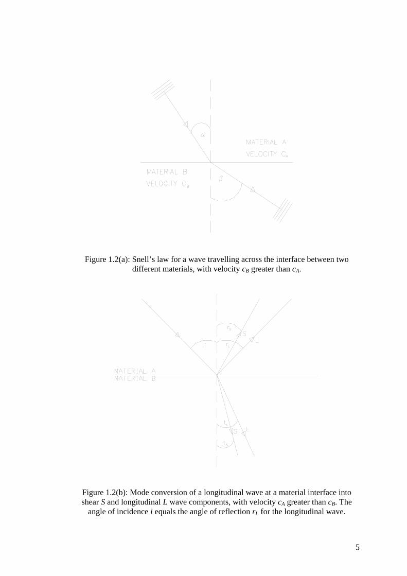
Figure 1.2(a): Snell’s law for a wave travelling across the interface between two different materials, with velocity cB greater than cB A.

Figure 1.2(b): Mode conversion of a longitudinal wave at a material interface into shear S and longitudinal L wave components, with velocity cA greater than cB. The

angle of incidence i equals the angle of reflection rB

L for the longitudinal wave.

5

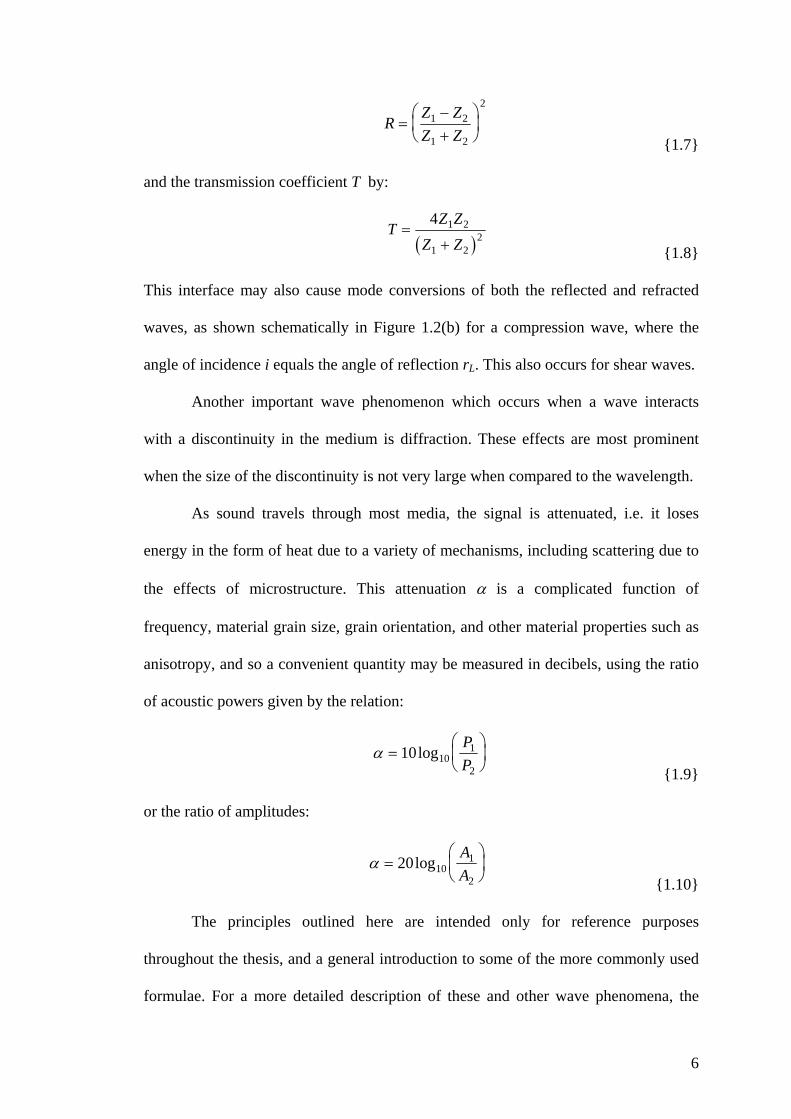
RZ ZZ Z

=−+

⎛⎝⎜

⎞⎠⎟1 2

1 2

2

{1.7}

and the transmission coefficient T by:

( )T

Z ZZ Z

=+

4 1 2

1 22

{1.8}

This interface may also cause mode conversions of both the reflected and refracted

waves, as shown schematically in Figure 1.2(b) for a compression wave, where the

angle of incidence i equals the angle of reflection rL. This also occurs for shear waves.

Another important wave phenomenon which occurs when a wave interacts

with a discontinuity in the medium is diffraction. These effects are most prominent

when the size of the discontinuity is not very large when compared to the wavelength.

As sound travels through most media, the signal is attenuated, i.e. it loses

energy in the form of heat due to a variety of mechanisms, including scattering due to

the effects of microstructure. This attenuation α is a complicated function of

frequency, material grain size, grain orientation, and other material properties such as

anisotropy, and so a convenient quantity may be measured in decibels, using the ratio

of acoustic powers given by the relation:

α =⎛⎝⎜

⎞⎠⎟10 10

1

2log

PP {1.9}

or the ratio of amplitudes:

α =⎛⎝⎜

⎞⎠⎟20 10

1

2log

AA {1.10}

The principles outlined here are intended only for reference purposes

throughout the thesis, and a general introduction to some of the more commonly used

formulae. For a more detailed description of these and other wave phenomena, the

6

reader is directed to any of the numerous works available on general optics and wave

theory [16].

1.4 Conventional ultrasonic testing

The use of sound to test engineering materials involves many different

techniques and applications, and most use some form of ultrasonic piezoelectric

contact probe [9,10,17]. These consist of a thin disc of a piezoelectric material, such

as quartz or lead-zirconate-titanate (PZT) with a metallised electrode on each face,

attached to a block of backing material. The construction of a typical piezoelectric

transducer is shown schematically in Figure 1.3(a). To generate ultrasonic waves, a

voltage is applied across these electrodes which causes the disc to vibrate due to the

piezoelectric effect. When acting as a receiver, an ultrasonic wave causing motion of

one of the faces of the piezoelectric element will produce a charge which may be

detected by a suitable amplifier. The majority of most conventional ultrasonic flaw

detectors and thickness gauges use piezoelectric transducers.

The transducers may be used in a number of different ways, the most common

being shown in Figure 1.3(b). When a single transducer is used as both a source and

receiver, this is known as pulse-echo. By employing two separate transducers, one as a

source and the other as a receiver, techniques such as pitch-catch (both transducers on

the same side of the sample) and through transmission (transducers on opposite sides

of the sample) may be used.

There are many different designs of piezoelectric transducer, which are usually

governed by the type of ultrasonic wave required. Longitudinal (compression) waves

7

Figure 1.3(a): Construction of a typical piezoelectric transducer.

Figure 1.4(b): Different transducer techniques.

8

and shear (transverse) waves may be easily generated by selecting a piezoelectric

element with the correct orientation. A transducer may have more than one element,

so that a single transducer may be used in pitch-catch rather than pulse-echo. By the

addition of a wedge at the correct angle, a variety of surface (Rayleigh) and plate

(Lamb) waves may be used in the sample under test. Focused transducers may be

similarly constructed by the addition of a suitable lens, or by using a curved

piezoelectric element.

1.5 Non-contact methods

To couple these vibrations into the material under examination, some form of

fluid couplant is usually used, or complete immersion in a water bath. This is the

major limitation of conventional ultrasonic probes, and there are many situations and

applications where contact with the specimen is undesirable, for example when the

sample is at elevated temperature, is moving rapidly in a production process, or the

material itself is toxic or radioactive. Many materials themselves are unsuitable for

use with fluid couplants, as they may be highly absorbent or easily corroded.

Fortunately there are methods of ultrasonic transduction which do not require

couplants or contact with the test material, and these will be described in the next

sections.

1.5.1 Laser generation of ultrasound

The use of pulsed lasers as sources of ultrasound has been well documented by

several authors [18-21], and will be described here as the technique is used

9

extensively throughout this thesis. When the surface of a sample is irradiated by a

pulsed laser, generation of ultrasonic transients may occur by one of three

mechanisms, determined by the optical power density and surface conditions. If the

power density is low (typically less than 107W/cm2), the absorption of radiation causes

rapid localised heating of the sample, making the irradiated area expand and generate

a stress (sound) wave which propagates through the medium, as shown in Figure

1.4(a). Since the majority of the stresses are transverse, i.e. in the plane of the sample

surface, this mechanism produces predominantly shear waves and is known as

thermoelastic generation. The corresponding surface displacement waveform is shown

in Figure 1.4(b), and consists of a small longitudinal component L, followed by a

larger step like shear wave arrival at S.

If the optical power density is increased (typically 107W/cm2 to109W/cm2), the

absorption of radiation causes a thin layer of the sample to vaporise or ablate. This

removal of material produces stresses normal to the sample surface by momentum

transfer, and so longitudinal waves are preferentially produced, as shown in Figure

1.5(a). This method of generation is known as ablation, and may be used in

conjunction with a layer of fluid or a constraining layer such as a glass cover slip to

enhance the longitudinal wave component. The corresponding surface displacement

waveform is shown in Figure 1.5(b), with now a much larger longitudinal transient L,

followed by a smaller shear step S. If the optical power density is increased further,

the vaporised material absorbs more energy and ionises into a plasma close to the

sample surface. The energy of the ions within the plasma, and hence the momentum

transfer into the sample, will increase with power density until the plasma shields the

surface from the incoming radiation, and no further gain in ultrasonic signal amplitude

is obtained. The interaction of the incoming laser pulse with the plasma is extremely

10

Figure 1.4(a): Laser generation of ultrasound by the thermoelastic mechanism.

Time (arbitrary)

Surfa

ce d

ispl

acem

ent (

arbi

trary

)

L

S

Figure 1.4(b): Theoretical displacement waveform for a thermoelastic source, with longitudinal L and shear S components. Adapted from Scruby and Drain [21].

11

Figure 1.5(a): Laser generation of ultrasound using the ablation mechanism.

Time (arbitrary)

Surfa

ce d

ispl

acem

ent (

arbi

trary

)

L

S

Figure 1.5(b): Theoretical displacement waveform for an ablative source, with longitudinal L and shear S components. Adapted from Scruby and Drain [21].

12

Figure 1.6(a): Laser generation of ultrasound using the air breakdown mechanism.

Time (arbitrary)

Surfa

ce d

ispl

acem

ent (

arbi

trary

)

L

S

Figure 1.6(b): Theoretical displacement waveform for an air breakdown source, with longitudinal L and shear S components. Adapted from Edwards et. al. [20]

13

complex [22], as various in-plasma detonation waves may be produced, and is outside

the scope of this study.

An alternative to this technique is to focus the incoming laser pulse to a point

some distance in front of the sample, and use a sufficiently high optical power to

ionise the air. This air breakdown source [20] produces a blast wave which imparts

momentum into the sample, and will preferentially generate longitudinal transients, as

shown in Figure 1.6(a), with the corresponding surface displacement waveform shown

in Figure 1.6(b).

1.5.2 Laser detection of ultrasound

Lasers have been used as detectors of displacement and surface motion for

many years [21,23-26], the most common type is probably the interferometer. Many

different designs are available, but the types most commonly used are (a) those that

measure displacement, by interfering the light returned from a surface (by reflection or

scattering) with a reference beam, and (b) those that operate as an optical spectrometer

to detect frequency shifts in the light returned from a surface, and hence act as

velocity detectors.

Most displacement interferometers are based on the Michelson interferometer,

shown schematically in Figure 1.7(a). The light source, usually a helium-neon (HeNe)

or argon-ion (Ar+) laser, is split into two beams, one of which goes to a static

reference mirror, the other to the surface under scrutiny which is moving due to the

influence of an ultrasonic wave. The two reflected beams are then recombined and

sent to a photodiode or some other optical detector. The intensity of the light received

14

Figure 1.7(a): The basic Michelson interferometer.

is dependent upon the phase difference between the reference and returned beam,

which is determined by the change in path lengths caused by motion of the surface. If

the range of surface motion is less than one wavelength, then the light intensity may

be measured directly, otherwise some form of counter is used to determine the number

of wavelengths moved.

The most common of the second type of device is the Fabry-Pérot

interferometer, which relies on the interference of multiple reflections of the light

returned from a sample to detect small changes in the frequency of this light due to

Doppler shift. The device uses a resonant optical cavity, shown schematically in

Figure 1.7(b), which consists of two parallel partially reflecting mirrors. This cavity

15

Figure 1.7(b): The resonant optical cavity of a Fabry-Pérot confocal interferometer.

Figure 1.7(c): The knife edge detector or beam deflector.

16

transmits most light when all the reflections are in phase, i.e. when there is an integer

number of wavelengths separating the mirrors. Any slight shift in frequency (caused

by motion of the sample surface) will cause the light intensity from the cavity to

change proportionally to the velocity of this motion. By using two identical curved

mirrors, separated exactly by their radius of curvature, the device is known as confocal

and is very insensitive to its orientation with the sample, and so is more practical.

Other forms of optical detector include the beam deflector and knife edge

detector, shown schematically in Figure 1.7(c). Motion of the sample surface will shift

the position of the reflected beam, so that either the amount of light detected past a

knife edge is varied, or the position of the beam on, say, a quadrant photodiode

connected to a differential amplifier is changed. This form of detector is most

sensitive to tilt of the surface under examination.

All laser based detectors have some significant limitations, however. Most

require good optical reflectivity from the surface under examination, and as real

samples tend to be optically rough, some form of surface preparation is required, and

this is not always practical. Most of the interferometers also require precise alignment,

a stable working environment, and (particularly the confocal Fabry-Pérot) can be

expensive due to the optical components required.

1.5.3 Non-contact transducers

There are several different non-contact transducers available with which a

laser based source or detector of ultrasound may be replaced. The electromagnetic

acoustic transducer (EMAT) [27,28] consists of a radio frequency (r.f.) coil in a static

magnetic field which permeates into the sample, as shown in Figure 1.8. When acting

17

as a receiver, an ultrasonic wave reaching the surface of the sample causes motion M

of the surface in the magnetic field B, generating an eddy current I which is picked up

by the coil. Generation is simply a reverse of this process, i.e. passing a current

through the coil to produce an ultrasonic wave. Both longitudinal and shear wave

EMATs may be constructed, as shown schematically in Figures 1.8(a) and 1.8(b)

respectively, by changing the orientation of the magnetic field with respect to the coil.

Another type of non-contact device is the capacitance transducer [17] (not to

be confused with the air-coupled capacitance detectors to be described later), and may

be used as both a source and detector of ultrasound. A polished flat electrode is placed

in close proximity to the surface of the sample which acts as the other electrode of a

capacitor, shown schematically in Figure 1.9. A bias voltage of typically a few

hundred volts is applied between the two electrodes. When used as a detector, an

ultrasonic wave causing motion of the sample surface will cause the electrode gap to

change, and thus the capacitance and charge on the two electrodes. This may be

detected by using a suitable charge sensitive amplifier. Often a thin polymer film is

used as the dielectric, instead of an air gap, producing a pseudo-contact device which

is easier to set up.

Both EMATs and this form of capacitance transducer have two significant

limitations. They require an electrically conducting sample, and so cannot be used on

most polymers and other non-conducting materials without preparation of the sample

surface with some form of conducting layer. They also require small stand-off

distances from the test specimen, typically a few mm for EMATs and a few µm for the

capacitance transducers.

18

Figure 1.8(a): A longitudinal wave EMAT.

Figure 1.8(b): A shear wave EMAT.

Figure 1.9: A capacitance transducer using air or a solid dielectric between the polished electrode and the conducting sample.

19

1.6 Air-coupled transducers

There has been much recent interest in the use of transducers that use air as

their coupling medium, as the restrictions associated with other devices do not occur.

Initially these devices were in the form of high frequency microphones [29], but in

general could not operate at frequencies in excess of 200-300 kHz. New designs [30],

however, can operate well into the MHz range. Air-coupled transducers may be

classified into two distinct groups, piezoelectric and capacitance (or electrostatic).

1.6.1 Piezoelectric air-coupled devices

Whilst being suited for direct coupling to a solid or liquid, most standard

piezoelectric transducers are inefficient when used with air as the coupling medium.

However, some success has been achieved using high powered driving circuitry and

amplifiers [31-32]. This inefficiency is due to the large impedance mismatch between

the air and the piezoelectric element. Using equations {1.6} and {1.8}, the

impedance, transmission coefficient and other acoustic properties are shown in Table

1.1 [9,10]. It can be seen that the majority of the acoustic energy is not transmitted and

so the efficiency of these devices in air is low. There are, however, several

mechanisms by which this efficiency may be improved. A metal membrane attached

to a 200kHz piezoelectric element has been used [33] to increase the coupling into air.

Layers of different material may also be attached to the front face of the transducer,

which match the device to air [34], ideally with an acoustic impedance ZL of:

20

Material

ρ

(kg.m-3)

cL

(m.s-1)

Z

(kg.m-3.s-1)

Twater

Tair

PZT-5 7700 3800 29.3 x106 183.6 x 10-3 5.6 x 10-5

BT 5300 5200 27.6 x106 193.8 x 10-3 6.0 x 10-5

Quartz 2650 5740 15.2 x106 323.7 x 10-3 10.9 x 10-5

PVDF 1760 2000 3.5 x106 834.2 x 10-3 46.9 x 10-5

Water (@20°C) 1000 1483 1.5 x106 1.0 111.3 x 10-5

Air (@20°C) 1.2 344 413.8 1.1 x 10-3 1.0

Table 1.1: Acoustical properties of some transducer materials [9,10].

Z Z ZL = 1 2. {1.11}

where Z1 and Z2 are the impedances of air and the piezoelectric element respectively.

These layers should be a quarter wavelength thick at the frequency of interest, and

they therefore reduce the overall bandwidth of the device. Materials such as Lucite

[35], silicone rubber [36], epoxy resin [37], aerogel [38] and ‘solid air’ (compacted

tiny air-filled spheres) [39] have been used, or a combination of different layers [40].

There has also been limited success when using air at very high pressure as the

coupling medium, with conventional piezoelectric devices, high gain amplifiers and

high powered driving circuitry [41]. Another method to improve the impedance

mismatch is to use a piezoelectric polymer which has an acoustic impedance closer to

that of air to construct the element, such as polyvinylidene difluoride (PVDF) [42-44],

or a copolymer [45].

Another technique is to modify conventional piezoceramic elements so that

their impedance is reduced, and thus their efficiency increased. These so called

21

Figure 1.10: Different connectivity composites, with the piezoelectric material shown

shaded.

piezocomposite materials are usually made from PZT and a filler material such as

epoxy resin. Piezocomposite materials have different properties depending on how the

material is modified, and are described in terms of the number of directions of

mechanical connectivity for both materials [46]. The different connectivities and

composite structures to which they apply are shown schematically in Figure 1.10.

Typical piezocomposite materials are 2-2 connectivity (alternate layers of ceramic

and filler) [47], and 1-3 connectivity (ceramic rods in a filler matrix). Perhaps the

22

most widely used piezocomposite material is 1-3 connectivity composite [35,48-53],

which is usually manufactured by the ‘slice and fill’ process [54], whereby slots are

machined into a disc of the required piezoceramic, and then filled with epoxy to

reduce the density and acoustic velocity of the material, and hence the impedance of

the element. The composite is then machined to an element of the required shape and

thickness for the frequency of interest. More recently, investigations into other

processing methods for piezocomposites have been performed [55], such as the

injection moulding of the piezoceramic into the required shape without the need for

machining.

1.6.2 Capacitance air-coupled devices

Electrostatic or capacitance transducers for operation in air [56] consist of a

contoured conducting backplate, over which a flexible dielectric film is placed. This

film is usually metallised so that a capacitor is created which has one rigid and one

flexible electrode. This type of device is shown schematically in Figure 1.11. Acting

as a receiver, a bias voltage is usually applied between the film and backplate

electrodes. An ultrasonic wave striking the film will cause it to vibrate, varying the air

gap behind it and thus the capacitance of the device. Variations in the charge on the

two electrodes may then be detected using a suitable charge sensitive amplifier.

Acting as ultrasonic generators, an alternating voltage applied to the device will cause

the charge on the electrodes to vary, and the dielectric film to move and produce an

ultrasonic wave in the surrounding air.

The majority of work to date concerning electrostatic air transducers has been

on different designs of contoured backplate. Traditionally, these have been

23

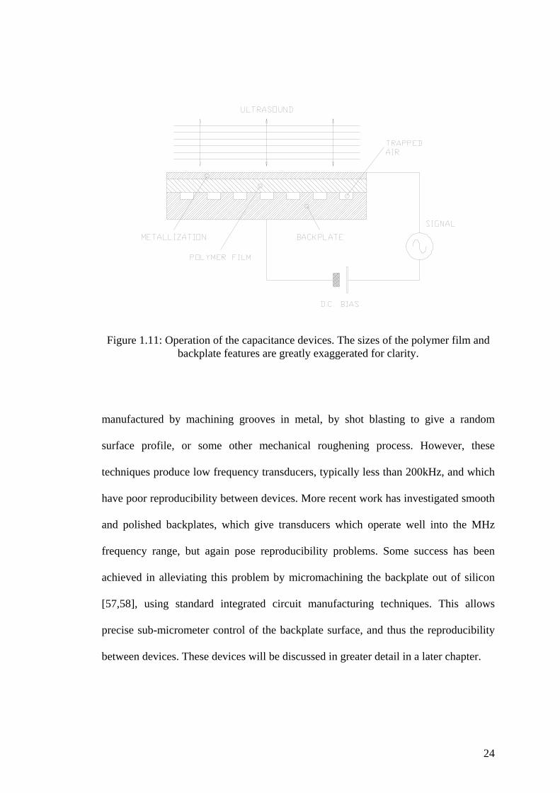
Figure 1.11: Operation of the capacitance devices. The sizes of the polymer film and backplate features are greatly exaggerated for clarity.

manufactured by machining grooves in metal, by shot blasting to give a random

surface profile, or some other mechanical roughening process. However, these

techniques produce low frequency transducers, typically less than 200kHz, and which

have poor reproducibility between devices. More recent work has investigated smooth

and polished backplates, which give transducers which operate well into the MHz

frequency range, but again pose reproducibility problems. Some success has been

achieved in alleviating this problem by micromachining the backplate out of silicon

[57,58], using standard integrated circuit manufacturing techniques. This allows

precise sub-micrometer control of the backplate surface, and thus the reproducibility

between devices. These devices will be discussed in greater detail in a later chapter.

24

1.7 Outline of the thesis

The work described in this thesis was driven by the recent advances in air-

coupled transducer technology, in that there seemed to be a lack of application of air-

coupled ultrasonics to existing practical situations. It was thus felt that this area of

work would present many interesting opportunities for research.

In Chapter 2, a capacitance or electrostatic device which used a backplate

micromachined from silicon was investigated. Laser generated ultrasound was used to

help characterise the device, and a more comprehensive study of laser generated

waveforms was performed. In Chapter 3, a range of piezoelectric air-coupled

transducers were evaluated in a similar fashion. These devices were 1-3 connectivity

composite designs, manufactured specifically as receivers. A novel instrumentation

system was developed, which used a pulsed laser as a source and an air-coupled

piezoelectric receiver. This preserved the non-contact nature of the experiments and

assisted in the characterisation of the devices. Details of the transducer construction

will be given, along with sample waveforms in aluminium and a comparison with a

standard pseudo-contacting displacement transducer, before extensive experimental

work in composite materials is presented.

In Chapter 4, a series of air-coupled capacitance devices with metallic

backplates were manufactured, and different methods of producing the backplates

(roughening, polishing and chemical etching) were evaluated. The effects of film

thickness and applied bias voltage were also investigated. Some of the devices were

designed to be used as sources, and so the practicalities of entirely air-coupled

ultrasonics were investigated. In Chapter 5, air-coupled Lamb waves were used to

estimate the thickness of thin metal plates and shim, using entirely non-contact

25

ultrasonics. The Lamb waves were either generated by the laser, or by an air-coupled

capacitance transducer. A computer program was written in FORTRAN to calculate

the theoretical dispersion curves in isotropic materials, and then two techniques were

employed to extract the dispersion relations and sample thickness data from the

air-coupled waveforms.

Chapter 6 presents details of how an entirely air-coupled ultrasonic system was

used to test a variety of materials, including pultruded glass-fibre reinforced polymer

(GRP) and carbon fibre reinforced polymer (CFRP) composites. This work used a pair

of silicon backplate air-coupled capacitance transducers, one as a source and one as a

receiver of ultrasound, to characterise samples using through transmission of bulk

waves and the propagation of Lamb waves. Waveforms were also obtained in other

materials such as perspex, expanded polyurethane foam and aluminium. A variety of

machined and delamination defects in these materials were evaluated with a C-

scanning technique which again used entirely air-coupled ultrasound.

Finally, another application of air-coupled ultrasonics was investigated in

Chapter 7. A pair of the micromachined silicon air-coupled capacitance transducers

was used to produce images of a variety of defects in thin plates using tomographic

reconstruction. In this technique, a sequence of regularly spaced ultrasonic waveforms

was used to build up a series of different views or projections through a defect at

different angles. A filtered back projection algorithm was then used to reconstruct a

cross sectional image of the defects.

26

1.8 References

[1] S. Schmidt, ‘Evidence for a spectral basis of texture perception in bat sonar’,

Nature 331, 617-619 (1988)

[2] N. Suga, ‘Biosonar and neural computation in bats’, Scientific American June

1990, 34-41 (1990)

[3] S. Stergiopoulos and A.T. Ashley, ‘Sonar system technology’, IEEE Journal of

Oceanic Engineering 18, (IEEE, New York, 1993)

[4] M. Lach and H. Embert, ‘An acoustic sensor system for object recognition’,

Sensors and Actuators A 25-27, 541-547 (1991)

[5] W.S.H. Munro, S. Pomeroy, M. Rafiq, H.R. Williams, M.D. Wybrow and

C. Wykes, ‘Ultrasonic vehicle guidance transducer’, Ultrasonics 28, 350-354

(1990)

[6] P. Kleinschmidt and V. Mágori, ‘Ultrasonic robotic sensors for exact short range

distance measurement’, Proc. 1985 IEEE Ultrason. Symp. 457-462 (1985)

[7] C.R. Hill (ed.), Physical principles of medical ultrasonics, (Ellis Horwood Ltd.,

Chichester, 1986)

[8] E.P. Papadakis, ‘Ultrasonic impulse-induced-resonance utilising damping for

adhesive disbond detection’, Mat. Eval. 36, 37-40 (1978)

[9] J. Krautkrämer and H. Krautkrämer, Ultrasonic testing of Materials, 4th edition,

(Springer-Verlag, Berlin,1990)

[10] R. Halmshaw, Non-destructive testing, (Edward Arnold, London, 1987)

[11] J. Blitz, Fundamentals of Ultrasonics, 2nd edition, (Butterworths, London,

1967)

27

[12] J.D. Achenbach, Wave propagation in elastic solids, (Elsevier Science

Publishers, Netherlands, 1990)

[13] I.A. Viktorov, Rayleigh and Lamb waves - Physical theory and applications,

(Plenum, New York, 1967)

[14] B.A. Auld, Acoustic fields and waves in solids: Volume II, (John Wiley Sons,

New York, 1973)

[15] G.S. Kino, Acoustic waves, (Prentice Hall, Englewood Cliffs NJ, 1987)

[16] F.A. Jenkins and H.E. White, Fundamentals of optics, 4th edition, (McGraw-Hill

Book Co., Singapore, 1981)

[17] W. Sachse and N.N. Hsu, ‘Ultrasonic transducers for materials testing and their

characterisation’, in Physical Acoustics - Principles and Methods, eds.

W.P. Mason and R.N. Thurston, (Academic, New York, 1979), Vol. XIV,

pp277-406

[18] R.M. White, ‘Generation of elastic waves by transient surface heating’, J. Appl.

Phys. 34, 3559-3567 (1963)

[19] D.A. Hutchins, ‘Ultrasonic generation by pulsed lasers’, in Physical Acoustics -

Principles and Methods, eds. W.P. Mason and R.N. Thurston, (Academic, New

York, 1988), Vol. XVIII, pp21-123

[20] C. Edwards, G.S. Taylor and S.B. Palmer, ‘Ultrasonic generation with a pulsed

TEA CO2 laser’, J. Phys. D: Appl. Phys. 22, 1266-1270 (1989)

[21] C.B. Scruby and L.E. Drain, Laser ultrasonics - techniques and applications,

(Adam Hilger, Bristol, 1990)

[22] M. von Allmen, Laser-beam interactions with materials - physical principles

and applications, (Springer-Verlag, Berlin, 1987)

28

[23] W.H. Steel, Interferometry, eds. A. Herzenberg and J.M. Ziman, (Cambridge

University Press, Cambridge, 1967)

[24] J.-P. Monchalin, ‘Optical detection of ultrasound’, IEEE Trans. Ultrason.,

Ferroelec., Freq. Contr. UFFC-33, 485-499 (1986)

[25] R. Jones and C. Wykes, Holographic and speckle interferometry - a discussion

of the theory, practice and application of the techniques, (Cambridge University

Press, Cambridge, 1989)

[26] J.W. Wagner, ‘Optical detection of ultrasound’, in Physical Acoustics -

Principles and methods, eds. W.P. Mason and R.N. Thurston, (Academic, New

York, 1990), Vol. XIX, pp201-266

[27] H.M. Frost, ‘Electromagnetic ultrasonic transducers: principles, practice and

applications’, in Physical Acoustics - Principles and methods, eds. W.P. Mason

and R.N. Thurston, (Academic, New York, 1979), Vol. XIV, pp179-276

[28] R.B. Thompson, ‘Physical properties of measurements with EMAT transducers’,

in Physical Acoustics - Principles and methods, eds. R.N. Thurston and

A.D. Pierce, (Academic, New York, 1990), Vol. XIX, pp157-200

[29] W. Kuhl, G.R. Schodder and F.-K. Schröder, ‘Condenser transmitters and

microphones with solid dielectric for airborne ultrasonics’, Acustica 4, 519-532

(1954)

[30] W. Manthey, N. Kroemer and V. Mágori, ‘Ultrasonic transducers and transducer

arrays for applications in air’, Meas. Sci. Techn. 3, 249-261 (1992)

[31] D.E. Chimenti and C.M. Fortunko, ‘Characterization of composite prepreg with

gas-coupled ultrasonics’, Ultrasonics 32, 261-264 (1994)

29

[32] A.J. Rogovsky, ‘Development and application of ultrasonic dry-contact and air-

contact C-scan systems for non-destructive evaluation of aerospace composites’,

Mat. Eval. 49, 1491-1497 (1991)

[33] M. Babic, ‘A 200-kHz ultrasonic transducer coupled to the air with a radiating

membrane’, IEEE Trans. Ultrason. Ferroelec. Freq. Contr. UFFC-38, 252-255

(1991)

[34] L.C. Lynnworth, ‘Ultrasonic impedance matching from solids to gases’, IEEE

Trans. Sonics, Ultrason. SU-12, 37-48 (1965)

[35] T.R. Gururaja, W.A. Schultze, L.E. Cross, R.E. Newnham, B.A. Auld and

Y.J. Wang, 'Piezoelectric composite materials for ultrasonic transducer

applications. Part I: Resonant modes of vibration of PZT rod-polymer

composites', IEEE Trans. Son. Ultrason. SU 32, 481-498 (1985)

[36] J.D. Fox, B.T. Khuri-Yakub and G.S. Kino, ‘High-frequency acoustic wave

measurements in air’, Proc. IEEE 1983 Ultrason. Symp., Vol.1, 581-584 (1983)

[37] J.D. Fox, B.T. Khuri-Yakub and G.S. Kino, ‘Acoustic resonator transducer for

operation in air’, Elec. Lett. 21, 694-696 (1985)

[38] O. Krauß, R. Gerlach and J. Fricke, 'Experimental and theoretical investigations

of SiO2-aerogel matched piezo-transducers', Ultrason. 32, 217-222 (1994)

[39] M. Teshigawara, F. Shibata and H. Teramoto, ‘High resolution (0.2mm) and fast

response (2ms) range finder for industrial use in air’, Proc. 1989 IEEE Ultrason.

Symp., 639-642 (1989)

[40] M. Tone, T. Yano and A. Fukumoto, 'High-frequency ultrasonic transducer

operating in air', Japan. J. Appl. Phys. 23, L436-L438 (1984)

[41] C.M. Fortunko, R.E. Schramm, C.M. Teller, G.M. Light, J.D. McColskey,

W.P. Dubé and M.C. Renken, ‘Pulse-echo gas-coupled ultrasonic crack

30

detection and thickness gaging’, Proc. Rev. Quant. Nondest. Eval. Vol. 14A and

14B, Ch. 312, 951-958 (1995)

[42] H. Kawai, ‘The piezoelectricity of poly(vinylidene fluoride)’, Japan. J. Appl.

Phys. 8, 975-976 (1969)

[43] M. Platte, ‘PVDF ultrasonic transducers for ultrasonic testing’, Ferroelectrics

115, 229-246 (1991)

[44] W. Manthey, N. Kroemer and V. Mágori, 'Ultrasonic transducers and transducer

arrays for applications in air', Meas. Sci. Technol. 3, 249-261 (1992)

[45] H. Ohigashi, K. Koga, M. Susuki and T. Nakamishi, ‘Piezoelectric and

ferroelectric properties of P(VDF-TrFE) copolymers and their application to

ultrasonic transducers’, Ferroelectrics 60, 263-276 (1984)

[46] R.E. Newnham, D.P. Skinner and L.E. Cross, 'Connectivity and piezoelectric-

pyroelectric composites', Mat. Res. Bull. 13, 525-536 (1978)

[47] T. Möckl, V. Màgori and C. Eccardt, 'Sandwich-layer transducer - a versatile

design for ultrasonic transducers operating in air', Sensors and Actuators A 21-

23, 687-692 (1990)

[48] W.A. Smith and B.A. Auld, ‘Modelling 1-3 composite piezoelectric: thickness

mode oscillations’, IEEE Trans. Ultrason. Ferroelec. Freq. Contr. UFFC-38,

40-47 (1991)

[49] T.R. Gururaja, W.A. Schulze, L.E. Cross and R.E. Newnham, 'Piezoelectric

composite materials for ultrasonic transducer applications. Part II: Evaluation of

ultrasonic medical applications', IEEE Trans. Son. Ultrason. SU 32, 499-513

(1985)

[50] M.I. Haller and B.T. Khuri-Yakub, ‘Micromachined 1-3 composites for

ultrasonic air transducers’, Rev. Sci. Instrum. 65, 2095-2098 (1994)

31

[51] J.A. Hossack and G. Hayward, 'Finite-element analysis of 1-3 composite

transducers', IEEE Trans. Ultrason. Ferroelec. Frequ. Contr. UFFC 38, 618-

629 (1991)

[52] G. Hayward, A. Gachagan, R. Hamilton, D.A. Hutchins and W.M.D. Wright,

‘Ceramic-epoxy composite transducers for non-contact ultrasonic applications’,

SPIE Symp. 1992, Vol. 1733, 49-56 (1992)

[53] G. Hayward and J.A. Hossack, 'Unidimensional modeling of 1-3 composite

transducers', J. Acoust. Soc. Am. 88, 599-608 (1990)

[54] H.P. Savakus, K.A. Klicker and R.E. Newnham, 'PZT-epoxy piezoelectric

transducer: a simplified fabrication procedure', Mat. Res. Bull. 16, 677-680

(1981)

[55] V.F. Janis and A. Safari, ‘Overview of fine-scale piezoelectric ceramic/polymer

composite processing’, J. Am. Ceram. Soc. 78, 2945-2955 (1995)

[56] H. Carr, W.S.H. Munro, M. Rafiq and C. Wykes, ‘Developments in capacitive

transducers’, Nondest. Test. Eval. 10, 3-14 (1992)

[57] K. Suzuki, K. Higuchi and H. Tanigawa, ‘A silicon electrostatic ultrasonic

transducer’, IEEE Trans. Ultrason., Ferroelec., Freq. Contr. UFFC-36, 620-627

(1989)

[58] D.W. Schindel, D.A. Hutchins, L. Zou and M. Sayer, ‘Capacitance devices for

the controlled generation of airborne ultrasonic fields’, Proc. IEEE 1992

Ultrason. Symp., 843-846 (1992)

32

Chapter 2: Studies of laser-generated ultrasound using an air-

coupled micromachined silicon capacitance transducer

2.1 Introduction

The work to be described in this chapter will investigate the detection of

laser-generated ultrasound in solid materials, using an air-coupled capacitance

transducer. These devices are usually made with metal backplates [1-4], and a more

detailed review will be given in Chapter 4. However, some of the problems

concerning capacitance devices for operation in air are lack of repeatability between

devices, and difficulty in producing identical surfaces for the backplate electrodes. In

an attempt to have more control over the surface properties of the backplate than are

available by mechanical machining techniques, integrated circuit manufacturing

techniques have been used to manufacture devices from silicon.

In the next section, a review of micromachined capacitance transducers will be

given, followed by construction details of the devices used in this study. The

following sections will then use laser-generated longitudinal waves in aluminium to

characterise the transducer, before a more detailed study of the various ultrasonic

waves from a laser source is conducted. The air-coupled waveforms will be compared

to those obtained from a capacitance transducer mentioned earlier in Chapter 1, which

uses the sample as one electrode.

2.1.1 Micromachined devices

Several different transducer designs using micromachined silicon have been

investigated. Suzuki et al. [5] developed devices which operated up to at least

500kHz, by using photolithographic techniques to etch an array of square holes into a

silicon wafer using ammonia solution. The conducting surface of the backplate was

33

produced by covering the pitted silicon with a 1µm layer of aluminium from an

electron gun. The dielectric layer was formed from SiO2 by chemical vapour

deposition (CVD), so that the insulating layer followed the contours of the surface.

The polymer membrane used was metallised 12µm polyester, with the metallised side

facing inwards so that the polymer film did not act as part of the dielectric. It was

shown that the hole dimensions had an effect on the low frequency response and the

sensitivity of the devices.

Other work by Schindel et al. [6-10] examined devices whose backplates

consisted of a regular array of circular pits, with only the polymer membrane and air

trapped behind it acting as the dielectric. The work to be described in this and

subsequent chapters used one or more of these devices and they will therefore be

described in more detail in the next section.

An alternative to etching silicon was attempted by Anderson et al. [11], where

polyamide ridges were deposited using photolithographic techniques onto a polished

aluminium surface, and a 5µm metallised polyethylene terephthalate (PET) membrane

used as the other electrode. The device relied on a well defined air gap between the

2.75µm high polymer ridges and the backplate surface. Thus the surface properties of

the aluminium were not of great importance, rather the tension of the membrane, as

the dominant mechanism of operation was flexing of the PET membrane. Measuring

the tension of polymer films used in capacitance devices has proved to be difficult.

The micromachined devices mentioned so far all used metallised flexible

polymer membranes as one electrode. This technique, however, allows for the

inclusion of unwanted particles between membrane and backplate during assembly of

the device. This may seriously effect the frequency response and operation of the

transducer, especially if the particles are of a similar size to the backplate surface

34

features. Kühnel and Hess [12] produced a range of devices entirely by

micromachining, using two separate silicon components. The first was a backplate

electrode with either grooves 10-12µm deep or holes 35-40µm deep, the second was a

membrane of silicon nitride 150nm thick. These devices were only 0.8mm square, and

operated at frequencies up to 20kHz. Haller and Khuri-Yakub [13] also manufactured

transducers using only micromachining, from a single piece of silicon. A layer of

silicon oxide was etched away beneath another layer of silicon nitride which acted as

the membrane electrode once it had been metallised with gold. Small pillars of the

etched SiO2 layer remained to support the membrane. These resonant devices operated

at frequencies of 1.8MHz and 4.5MHz, although more recently a 9.2MHz device has

been reported by the same authors [14].

The work described so far has concentrated mainly on the manufacture of the

devices themselves, rather than applications using air-coupled ultrasound [15]. The

experiments described in this chapter were the first to use a pulsed laser and a

capacitance air-coupled detector for non-contact ultrasonics, and the results have been

published [16].

2.1.2 Construction of the micromachined silicon air-coupled transducer

The transducer used in this work is one of the air-coupled capacitance type

devices mentioned earlier in Chapter 1, made by David Schindel at the Department of

Physics, Queens University Canada. The construction detail of the transducer is shown

schematically in Figure 2.1, and was manufactured as follows [10]. A polished (110)

35

Figure 2.1: Detail of the micromachined silicon backplate.

silicon wafer was coated with masking layers of silicon nitride and silicon oxide, plus

a layer of photoresist. The photoresist was exposed using photolithographic

techniques through a mask consisting of a uniform grid of 40µm diameter holes, with

the hole centres 80µm apart. The silicon oxide circles were then removed using a

hydrofluoric acid etch, and the silicon nitride circles etched with phosphoric acid. The

silicon substrate was finally etched with potassium hydroxide, to a self limiting depth

of 18µm. The contoured backplate was then coated with 1000Å of gold to make a

conducting surface. The dielectric and upper electrode consisted of a 7.6µm Kapton

polyimide membrane, metallized on the outer side with aluminium. This prototype

device had an active area of 10x7mm.

36

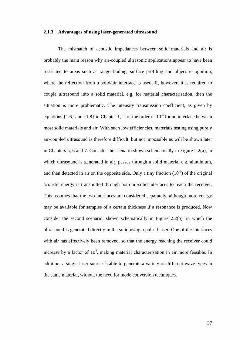
2.1.3 Advantages of using laser-generated ultrasound The mismatch of acoustic impedances between solid materials and air is

probably the main reason why air-coupled ultrasonic applications appear to have been

restricted to areas such as range finding, surface profiling and object recognition,

where the reflection from a solid/air interface is used. If, however, it is required to

couple ultrasound into a solid material, e.g. for material characterisation, then the

situation is more problematic. The intensity transmission coefficient, as given by

equations {1.6} and {1.8} in Chapter 1, is of the order of 10-4 for an interface between

most solid materials and air. With such low efficiencies, materials testing using purely

air-coupled ultrasound is therefore difficult, but not impossible as will be shown later

in Chapters 5, 6 and 7. Consider the scenario shown schematically in Figure 2.2(a), in

which ultrasound is generated in air, passes through a solid material e.g. aluminium,

and then detected in air on the opposite side. Only a tiny fraction (10-8) of the original

acoustic energy is transmitted through both air/solid interfaces to reach the receiver.

This assumes that the two interfaces are considered separately, although more energy

may be available for samples of a certain thickness if a resonance is produced. Now

consider the second scenario, shown schematically in Figure 2.2(b), in which the

ultrasound is generated directly in the solid using a pulsed laser. One of the interfaces

with air has effectively been removed, so that the energy reaching the receiver could

increase by a factor of 104, making material characterisation in air more feasible. In

addition, a single laser source is able to generate a variety of different wave types in

the same material, without the need for mode conversion techniques.

37

Figure 2.2(a): Through transmission in air using two air-coupled transducers. Values

shown are approximate fractions of the original energy.

Figure 2.2(b): Improved through transmission using a laser source. Values shown are

approximate fractions of the original energy.

38

2.2 Studies of laser-generated through transmission waveforms

Experiments were performed to detect laser-generated waveforms in a variety

of solid materials, using the equipment shown schematically in Figure 2.3(a).

Ultrasound was generated in the samples using a Lumonics ‘Mini-Q’ Q-switched

Nd:YAG laser, operating at a wavelength of 1064nm in the near infra-red spectrum,

and delivering pulses of 4ns duration with a maximum energy of 120mJ per pulse. The

beam was directed onto the sample using various optics to give an ablative source

approximately 2mm in diameter. Signals were then detected by the air-coupled device,

to which a 100V d.c. bias was applied via a Cooknell CA6/C charge amplifier with

SU2/C power supply. The resultant time domain waveforms were captured using a

Tektronix 540 TDS digital oscilloscope, and transferred to an IBM PS/2 Model 30 286

PC via an IEEE-488/GPIB interface for storage and analysis. For more detailed

equipment specifications, see Appendix A. Unless stated otherwise, the air gap

between sample and transducer was 10mm, although larger separations were possible.

2.2.1 Characterising the air-coupled capacitance transducer

To provide some form of calibration waveform against which to compare the

air-coupled devices, a contact capacitance probe was also used to detect the

laser-generated ultrasound for the same generation conditions. This is shown

schematically in Figure 2.3(b), and consisted of a steel sphere, in an insulated case,

used as one electrode of a capacitor with the other electrode being the sample itself.

Note that due to the use of a spherical electrode, tilt of this device is not critical, and

39

Figure 2.3(a): Schematic diagram of the experimental apparatus.

Figure 2.3(b): The contact capacitance device used for comparison.

40

acts as a point receiver at most angles. A film of polymer 5µm thick was used as a

dielectric between the two electrodes, and a bias voltage of 100V was applied between

the sphere and the sample. This type of device is a well characterised displacement

sensor [17], and gives a linear response (to within 0.5%) up to frequencies of at least

30MHz. The same amplifier, bias unit and waveform storage facilities were used with

both transducers.

The first experiments compared the signals detected by the silicon electrostatic

transducer to those detected by the contacting capacitance device for normal

displacement of an aluminium surface caused by bulk wave propagation. The surface

motion recorded in an 86.0mm thick aluminium sample is shown in Figure 2.4(a) for an

ablative source, detected by the contact device and showing the longitudinal arrival

only. 128 averages were used to reduce the level of background noise. This thickness

of aluminium was chosen so that the longitudinal and shear waves were well separated

in time, to allow the transducers to reach an equilibrium state between echoes. The

waveform has the characteristic sharp monopolar longitudinal arrival associated with a

laser-generated ablative source, shown earlier in Figure 1.5(b) in Chapter 1. To

illustrate the bandwidth present in this signal, a fast Fourier transform (FFT) of the

waveform is shown in Figure 2.4(b), which indicates that the device was broadband up

to a frequency of 10MHz, which was the upper frequency limit of the charge amplifier.

The effects of the higher frequencies are reduced due to attenuation in the sample and

diffraction. The corresponding waveform for the electrostatic air transducer, the result

of just 16 signal averages, is shown in Figure 2.5(a), with the FFT of the longitudinal

arrival in Figure 2.5(b). This indicates that the air transducer had a much narrower

bandwidth, with a reduced response at both low and high frequencies when compared

to the contact device. This may be attributed in part to the attenuation in air of high

41

-0.5 0.0 0.5 1.0 1.5 2.0 2.5 3.0 3.5 4.0Time (µs)

-10.0

-8.0

-6.0

-4.0

-2.0

0.0

2.0

Ampl

itude

(mV)

Figure 2.4(a): Longitudinal wave through 86.0mm aluminium detected by the contact transducer.

0.0 1.0 2.0 3.0 4.0 5.0 6.0 7.0 8.0 9.0 10.Frequency (MHz)

0

0.0

0.1

0.2

0.3

0.4

0.5

0.6

0.7

0.8

0.9

1.0

Nor

mal

ised

FFT

am

plitu

de


42

-1.0 0.0 1.0 2.0 3.0 4.0 5.0 6.0 7.0 8.0Time (µs)

-40.0

-30.0

-20.0

-10.0

0.0

10.0

20.0

30.0

Ampl

itude

(mV)

Figure 2.5(a): Longitudinal arrival through 86.0mm aluminium detected using the air-coupled micromachined capacitance device.

0.0 1.0 2.0 3.0 4.0 5.0 6.0 7.0 8.0 9.0 10.Frequency (MHz)

0

0.0

0.1

0.2

0.3

0.4

0.5

0.6

0.7

0.8

0.9

1.0

Nor

mal

ised

FFT

am

plitu

de

Figure 2.5(b): Frequency spectrum of the waveform in Figure 2.5(a).

43

frequencies, the different characteristics of the transducer, and the larger active area of

the air-coupled device, as the contact transducer is effectively a point receiver. In

addition, the applied bias voltage was restricted to 100V by the charge amplifier, and

so the recommended 400V could not be used [10] to obtain a wider bandwidth.

A more typical waveform with multiple reflections in a thinner (12.8mm)

sample of aluminium is shown in Figure 2.6(a) for the contact device. L1, L2 etc. are

the longitudinal wave arrivals, with a shear wave arrival at S. The features at M1, M2

etc. are the longitudinal mode conversions of the first shear wave arrival at S, and R is

a reflection from the edge of the sample. Figure 2.6(b) shows the corresponding signal

received by the air-coupled transducer, and all the major features in the contact

transducer waveform (L1, S, M1 etc.) have been detected.

The signal in Figure 2.5(a) is the response of the air-coupled device to what is

essentially a delta function from the laser, and so the spectrum in Figure 2.5(b) may be

thought of as the overall frequency response of the device. If the FFT of the contact

device waveform of Figure 2.6(a) is multiplied by the normalised ‘response’ spectrum

in Figure 2.5(b), and the result inverse Fourier transformed, the waveform shown in

Figure 2.6(c) is produced. This is effectively the broadband displacement waveform of

Figure 2.6(a) filtered over the narrower frequency range detected by the air-coupled

transducer. Figure 2.6(d) shows the differentiation of the displacement waveform

Figure 2.6(a), and thus describing the velocity of the surface. A comparison of Figures

2.6(b) and (c) shows a degree of similarity, with all the main features (L1, S, M1 etc.)

clearly visible. It could therefore be assumed that the air-coupled device operated as a

sensor which gave a good representation of the displacement of the sample surface,

but with a reduced bandwidth.

44

0.0 2.0 4.0 6.0 8.0 10.0 12.0 14.0 16.0 18.0 20.0

Time (µs)

-0.07

-0.06

-0.05

-0.04

-0.03

-0.02

-0.01

0.00

0.01

Ampl

itude

(mV)

L1

S1

L2

M1

L3

L4

L5

M2 M3 R1

Figure 2.6(a): Waveform through 12.8mm of aluminium detected using the contact transducer, showing the surface displacement.

16.0 18.0 20.0 22.0 24.0 26.0 28.0 30.0 32.0 34.0 36.0Time (µs)

-0.25

-0.20

-0.15

-0.10

-0.05

0.00

0.05

0.10

0.15

Ampl

itude

(mV)

L1

L2

L3 L4 L5

S1 M1

M2 M3

Figure 2.6(b): Waveform through 12.8mm of aluminium, detected using the micromachined air-coupled capacitance transducer.

45

0.0 2.0 4.0 6.0 8.0 10.0 12.0 14.0 16.0 18.0 20.0Time (µs)

-6.0

-4.0

-2.0

0.0

2.0

4.0

6.0

8.0

10.0

12.0

Ampl

itude

(mV)

L1

S1

L2

M1

L3 M3

Figure 2.6(c): Waveform in Figure 2.6(a) ‘filtered’ over the range of frequencies shown in Figure 2.5(b).

0.0 2.0 4.0 6.0 8.0 10.0 12.0 14.0 16.0 18.0 20.0 22.0Time (µs)

-2.5

-2.0

-1.5

-1.0

-0.5

0.0

0.5

1.0

1.5

2.0

Ampl

itude

(mV)

L1 S1

L2

M1

L3

M2

L4

R1 L5

M3

Figure 2.6(d): Contact capacitance transducer waveform after differentiation, showing the velocity of the surface.

46

Another experiment was conducted in which the optical power density at the

aluminium surface was gradually increased, so that the generation mechanism

changed from thermoelastic expansion to ablation. A selection of waveforms is

presented in Figure 2.7 for (a) the contact device and (b) the air-coupled transducer.

Again, there is good correlation between the two devices. The step like shear arrival

S1 is present in most waveforms and optical densities, and the monopolar longitudinal

arrival L1 and echo L2 increasingly dominate the signal as the source becomes more

ablative.

The combination of a laser source and an air-coupled receiver may be used to

test many different materials. Similar waveforms to those shown in Figures 2.6 for

aluminium were also obtained in samples of brass and steel, with slight variations in

waveform shape which may be attributed to the differences in microstructure, elastic

properties and thermal characteristics of the materials. A typical signal in 10mm of

steel is shown in Figure 2.8(a), where it can be seen that the shear wave S1 is far less

prominent when compared to Figure 2.6(b). Waveforms were also obtained in samples

of perspex (polymethylmethacrylate) by replacing the Nd:YAG laser with a Lumonics

‘Lasermark’ series Model 630 CO2 TEA (Transversely Excited at Atmospheric

pressure) laser, which had a pulse duration of 100ns and a maximum energy of 8J.

This laser operated at a wavelength of 10.6µm in the far infra-red spectrum, where

absorption in this polymer, which readily transmits visible and near infra-red light, is

high. A typical signal in a 25mm thick sample is shown in Figure 2.8(b), where the

shear step S1 is the dominant feature. The generation mechanism was predominantly

thermoelastic, due to the improved absorption at this wavelength.

47

L1

S1

L2

Figure 2.7(a): Signals obtained using an increasing optical power density, detected

using the contact device.

48

L1

S1

L2

Figure 2.7(b): Signals obtained using an increasing optical power density, detected

using the micromachined air-coupled capacitance transducer.

49

16.0 18.0 20.0 22.0 24.0 26.0 28.0 30.0 32.0 34.0 36.0Time (µs)

-0.25

-0.20

-0.15

-0.10

-0.05

0.00

0.05

0.10

0.15

Ampl

itude

(vol

ts)

L1

L2 L3 L4

S1

M1

M2 M3

Figure 2.8(a): Typical laser-generated waveform in 10mm thick steel, detected using the air-coupled capacitance transducer.

-4.0 0.0 4.0 8.0 12.0 16.0 20.0 24.0 28.0 32.0 36.0Time (µs)

-6.0

-4.0

-2.0

0.0

2.0

4.0

6.0

Ampl

itude

(mV)

L1

S1

L2

Figure 2.8(b): Typical laser-generated waveform in 25mm thick Perspex, detected using the air-coupled capacitance transducer.

50

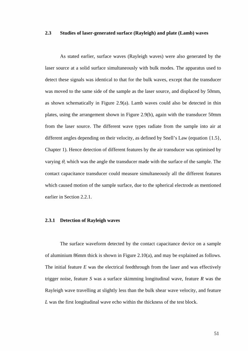
2.3 Studies of laser-generated surface (Rayleigh) and plate (Lamb) waves

As stated earlier, surface waves (Rayleigh waves) were also generated by the

laser source at a solid surface simultaneously with bulk modes. The apparatus used to

detect these signals was identical to that for the bulk waves, except that the transducer

was moved to the same side of the sample as the laser source, and displaced by 50mm,

as shown schematically in Figure 2.9(a). Lamb waves could also be detected in thin

plates, using the arrangement shown in Figure 2.9(b), again with the transducer 50mm

from the laser source. The different wave types radiate from the sample into air at

different angles depending on their velocity, as defined by Snell’s Law (equation {1.5},

Chapter 1). Hence detection of different features by the air transducer was optimised by

varying θ, which was the angle the transducer made with the surface of the sample. The

contact capacitance transducer could measure simultaneously all the different features

which caused motion of the sample surface, due to the spherical electrode as mentioned

earlier in Section 2.2.1.

2.3.1 Detection of Rayleigh waves

The surface waveform detected by the contact capacitance device on a sample

of aluminium 86mm thick is shown in Figure 2.10(a), and may be explained as follows.

The initial feature E was the electrical feedthrough from the laser and was effectively

trigger noise, feature S was a surface skimming longitudinal wave, feature R was the

Rayleigh wave travelling at slightly less than the bulk shear wave velocity, and feature

L was the first longitudinal wave echo within the thickness of the test block.

51

Figure 2.9(a): Apparatus for detecting Rayleigh waves.

Figure 2.9(b): Apparatus for detecting Lamb waves.

52

-4.0 0.0 4.0 8.0 12.0 16.0 20.0 24.0 28.0 32.0 36.0Time (µs)

-20.0

-15.0

-10.0

-5.0

0.0

5.0

10.0

15.0

20.0

Ampl

itude

(mV)

E

S

R

L

Figure 2.10(a): Surface waves in aluminium detected by the contact transducer.

-4.0 0.0 4.0 8.0 12.0 16.0 20.0 24.0 28.0 32.0 36.0Time (µs)

-8.0

-6.0

-4.0

-2.0

0.0

2.0

4.0

Ampl

itude

(mV)

L

Figure 2.10(b): Surface waves in aluminium at an angle of 0°, detected using the air-coupled capacitance transducer.

53

-4.0 0.0 4.0 8.0 12.0 16.0 20.0 24.0 28.0 32.0 36.0Time (µs)

-12.0

-10.0

-8.0

-6.0

-4.0

-2.0

0.0

2.0

4.0

6.0

8.0

Ampl

itude

(mV)

S

Figure 2.10(c): Surface waves in aluminium at an angle of 3°, detected using the air-coupled capacitance transducer.

-4.0 0.0 4.0 8.0 12.0 16.0 20.0 24.0 28.0 32.0 36.0Time (µs)

-40.0

-30.0

-20.0

-10.0

0.0

10.0

20.0

30.0

40.0

50.0

Ampl

itude

(mV)

R

Figure 2.10(d): Surface waves in aluminium at an angle of 6°, detected using the air-coupled capacitance transducer.

54

The experiment was then repeated using the air-coupled capacitance transducer, with

results for various angles of θ shown optimised in Figure 2.10 for (b) the longitudinal

reflection L at θ=0°, (c) the surface skimming longitudinal wave S at θ=3°, and (d) the

Rayleigh wave R at θ=6°.

2.3.2 Detection of Lamb waves

A plate of aluminium 0.69mm thick was used as the sample, and a typical

normal displacement waveform is shown in Figure 2.11, detected using the contact

capacitance probe. The symmetric s modes and asymmetric a modes are clearly

visible, and show some dispersion due to the thickness of the plate and the range of

frequencies present, particularly for the a0 mode. Some higher order modes are also

present.

By replacing the contact device with the micromachined air-coupled

transducer, the various Lamb wave modes could also be detected in air. A selection of

waveforms at different angles of the detector is shown in Figure 2.12(a) to (e). At

θ=2°, the symmetric mode is clearly visible, but reduces in amplitude at θ=5°, and is

not visible at all at θ=10°. This was expected, as the s0 mode in thin plates has a

velocity approaching the sheet velocity (approximately the longitudinal velocity in the

material), and hence will radiate into air at small angles. The higher frequency

asymmetric vibrations become more prominent at θ=5-10°, and at larger angles the

frequency content of this asymmetric mode clearly decreases.

Lamb waves could also generated and detected in a 1.5mm thick sheet of

perspex, using the CO2 laser described earlier as a source of ultrasound. A typical

55

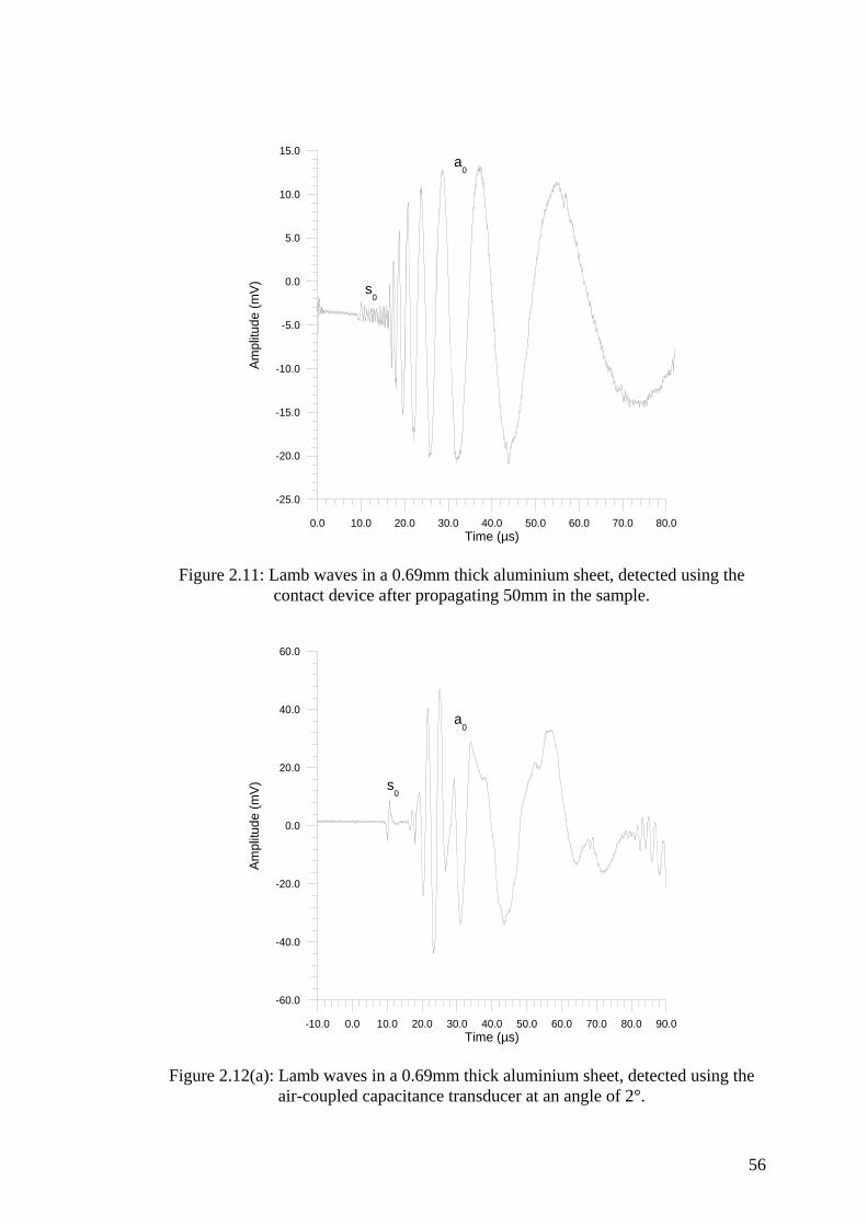
0.0 10.0 20.0 30.0 40.0 50.0 60.0 70.0 80.0Time (µs)

-25.0

-20.0

-15.0

-10.0

-5.0

0.0

5.0

10.0

15.0

Ampl

itude

(mV) s

0

a0

Figure 2.11: Lamb waves in a 0.69mm thick aluminium sheet, detected using the contact device after propagating 50mm in the sample.

-10.0 0.0 10.0 20.0 30.0 40.0 50.0 60.0 70.0 80.0 90.0Time (µs)

-60.0

-40.0

-20.0

0.0

20.0

40.0

60.0

Ampl

itude

(mV) s

0

a0

Figure 2.12(a): Lamb waves in a 0.69mm thick aluminium sheet, detected using the air-coupled capacitance transducer at an angle of 2°.

56

-10.0 0.0 10.0 20.0 30.0 40.0 50.0 60.0 70.0 80.0 90.0Time (µs)

-60.0

-40.0

-20.0

0.0

20.0

40.0

60.0

Ampl

itude

(mV)

s0

a0

Figure 2.12(b): Lamb waves in a 0.69mm thick aluminium sheet, detected using the air-coupled capacitance transducer at an angle of 5°.

-10.0 0.0 10.0 20.0 30.0 40.0 50.0 60.0 70.0 80.0 90.0Time (µs)

-100.0

-80.0

-60.0

-40.0

-20.0

0.0

20.0

40.0

60.0

80.0

100.0

120.0

Ampl

itude

(mV)

a0

Figure 2.12(c): Lamb waves in a 0.69mm thick aluminium sheet, detected using the air-coupled capacitance transducer at an angle of 10°.

57

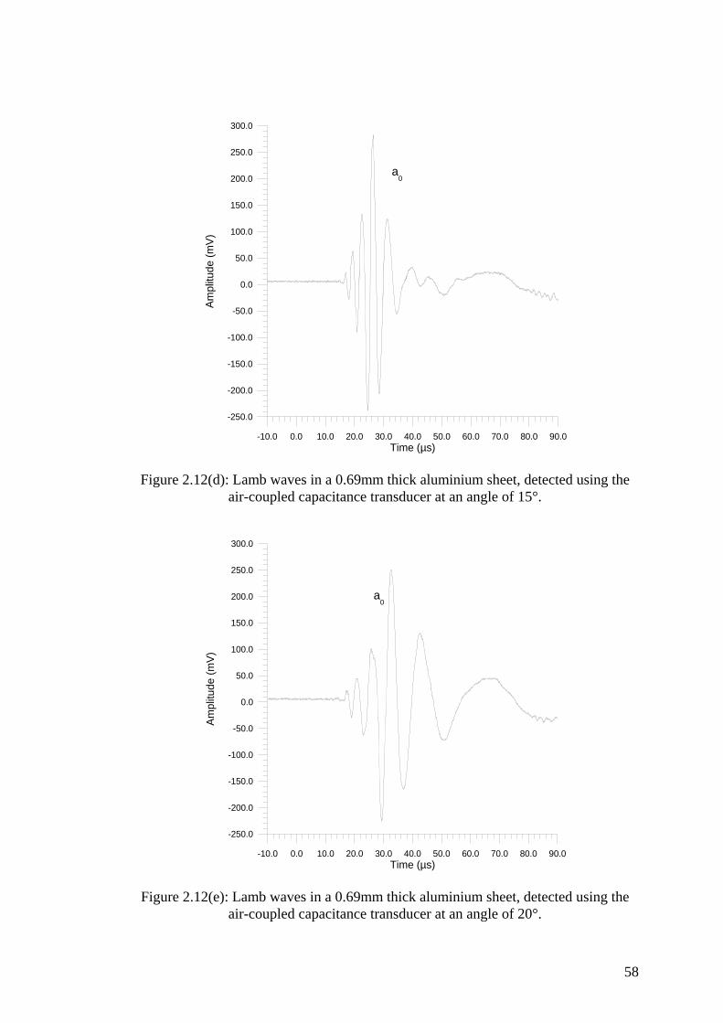
-10.0 0.0 10.0 20.0 30.0 40.0 50.0 60.0 70.0 80.0 90.0Time (µs)

-250.0

-200.0

-150.0

-100.0

-50.0

0.0

50.0

100.0

150.0

200.0

250.0

300.0

Ampl

itude

(mV)

a0

Figure 2.12(d): Lamb waves in a 0.69mm thick aluminium sheet, detected using the air-coupled capacitance transducer at an angle of 15°.

-10.0 0.0 10.0 20.0 30.0 40.0 50.0 60.0 70.0 80.0 90.0Time (µs)

-250.0

-200.0

-150.0

-100.0

-50.0

0.0

50.0

100.0

150.0

200.0

250.0

300.0

Ampl

itude

(mV)

a0

Figure 2.12(e): Lamb waves in a 0.69mm thick aluminium sheet, detected using the air-coupled capacitance transducer at an angle of 20°.

58

-10.0 0.0 10.0 20.0 30.0 40.0 50.0 60.0 70.0 80.0 90.0Time (µs)

-80.0

-60.0

-40.0

-20.0

0.0

20.0

40.0

60.0

80.0

Ampl

itude

(mV)

s0

a0

Figure 2.13: Lamb waves in a 1.5mm thick perspex sheet, detected using the air-coupled capacitance transducer at an angle of 12°.

signal is shown in Figure 2.13 at a transducer angle of θ=10°, where both the a0 and s0

modes are clearly visible.

2.4 Discussion

It is interesting to note that despite the very high frequencies present in the

laser-generated bulk waves, the device seemed to have an upper frequency limit of

approximately 2MHz, as shown in Figure 2.5(b). This feature has also been noted in

other work on the same capacitance devices operating in air [10], when used as either

transmitters or receivers of ultrasound to frequencies of up to 4MHz. This suggests

59

that there is some major limiting factor to the upper frequency limit of this device, and

perhaps air-coupled ultrasound in general.

This is most probably the effects of absorption and attenuation in air, which

has been extensively studied by many authors. Typical reviews of this subject are

those by Bass et al. [18] and Hickling and Marin [19]. Hickling gives the governing

equation as:

p z p eOz( ) . .= −α {2.1}

where pO is the r.m.s. pressure at some initial location, p(z) is the pressure amplitude

after travelling z metres, and α is the attenuation coefficient. Bass et al. further

characterised this coefficient and state that α may be closely approximated by:

α α α α= + +cr vib O vib N, , {2.2}

where αcr is a combination of classical absorption and rotational relaxation, and αvib,j

is the absorption due to the vibrational relaxation of both oxygen O and nitrogen N.

αcr is given by:

α cro o

TT

PP

f= ×⎛⎝⎜

⎞⎠⎟

⎛⎝⎜

⎞⎠⎟−183 10 11

12

12 2.

{2.3}

where T and To are the actual and reference temperatures respectively, P and Po are

the actual and reference pressures respectively, and f is the frequency. αvib,j is given

by:

( )( ) ( )

απ θ θ

θvib j

j jT

T

r j

r j

Xc

T e

e

f f

f f

j

j,

,

,

. ..

=− +

−

−

435 1 1

2

2

2

2

{2.4}

where Xj is the molar fraction, θj is the vibrational temperature, and fr,j is the

vibrational relaxation frequency for both oxygen and nitrogen. Equation {2.4} is also

60

affected by humidity, and becomes increasingly complex, and further investigation of

this topic is outside the scope of this study. In most practical situations, where

accurate knowledge of the attenuation caused by air is required, it may be simpler to

experimentally measure values of α as shown in Section 1.3. Hickling gives typical

theoretical values of 10-3m-1 at 1kHz and 10m-1 at 1MHz in air at 30°C. Hickling also

defines an extinction distance de, a distance in air over which the amplitude of a signal

is reduced to 1/e of its original value. This may be approximated at a frequency f by:

dfe =×5 1013

2 {2.5}

where de is in mm. For the sample-receiver distances (de) of 10mm used in the

experiments described in this chapter, f is 2.24MHz, which was approximately the

upper frequency of the devices. It was not practical to use smaller air gaps due to the

construction of the capacitance transducers. Interestingly, for the 9.2MHz air-coupled

device described earlier [10], de is approximately 0.6mm rather than the 5mm air gap

used, probably for similar reasons. For practical air-coupled NDT, over distances of

10mm or more, devices operating at frequencies in excess of 2.5-3MHz are therefore

at a distinct disadvantage.

2.5 Conclusions

The work described in this chapter has shown that air-coupled capacitance

transducers, which have been micromachined from silicon, are well suited to the

detection of a variety of laser-generated ultrasonic waveforms. The response of the

transducer to bulk waves, surface waves in thick samples, and Lamb waves in thin

plates was compared to the response of a wideband contact transducer. Bulk waves

61

were used to partly characterise the air-coupled device, which was found to operate as

a sensor which gave a good representation of the displacement of the sample surface,

but with a reduced bandwidth. Due to the present lack of a standard air-coupled

transducer or high-frequency microphone operating in the MHz range, any sensitivity

measurements of the silicon device would be uncalibrated and of little value, and so a

more complete characterisation of the air-coupled capacitance device should form an

important part of any work in the future.

2.6 References

[1] M. Rafiq and C. Wykes, 'The performance of capacitive ultrasonic transducers

using v-grooved backplates', Meas. Sci. Technol. 2, 168-174 (1991)

[2] W.S.H. Munro and C. Wykes, ‘Arrays for airborne 100kHz ultrasound’,

Ultrasonics 32, 57-64 (1994)

[3] W.S.H. Munro, S. Pomeroy, M. Rafiq, H.R. Williams, M.D. Wybrow and C.

Wykes, ‘Ultrasonic vehicle guidance transducer’, Ultrasonics 28, 350-354

(1990)

[4] H. Carr and C. Wykes, 'Diagnostic measurements in capacitive transducers',

Ultrasonics 31, 13-20 (1993)

[5] K. Suzuki, K. Higuchi and H. Tanigawa, ‘A silicon electrostatic ultrasonic

transducer’, IEEE Trans. Ultrason. Ferroelec. Freq. Contr. UFFC-36, 620-627

(1989)

[6] D.W. Schindel, D.A. Hutchins, L. Zou and M. Sayer, ‘Capacitance devices for

the generation of air-borne ultrasonic fields’, Proc. 1992 IEEE Ultrason. Symp.

843-846 (1992)

62

[7] D.W. Schindel, D.A. Hutchins, L. Zou and M. Sayer, ‘Capacitance transducers

for generating ultrasonic fields in liquids and gases’, Proc. IEE International

Conference on Acoustic Sensing and Imaging ASI’93, 7-12 (1993)

[8] D.W. Schindel, D.A. Hutchins, L. Zou and M. Sayer, ‘Micromachined

capacitance transducers for air-borne ultrasonics’, Proc. Ultrasonics Int. Conf.

1993, 675-678 (1993)

[9] D.W. Schindel and D.A. Hutchins, ‘Air-coupled ultrasonic transducer’, U.S.

Patent 5,287,331, February 1994

[10] D.W. Schindel, D.A. Hutchins, L. Zou and M. Sayer, ‘The design and

characterization of micromachined air-coupled capacitance transducers’, IEEE

Trans. Ultrason. Ferroelec. Freq. Contr. UFFC-42, 42-50 (1995)

[11] M.J. Anderson, J.A. Hill, C.M. Fortunko, N.S. Dogan and R.D. Moore,

‘Broadband electrostatic transducers: Modeling and experiments’, J. Acoust.

Soc. Am. 97, 262-272 (1995)

[12] W. Kühnel and G. Hess, ‘A silicon condenser microphone with structured back

plate and silicon nitride membrane’, Sensors and Actuators A, 30, 251-258

(1992)

[13] M.I. Haller and B.T. Khuri-Yakub, ‘A surface micromachined electrostatic

ultrasonic air transducer’, Proc. IEEE 1994 Ultrason. Symp. Ch. 395, 1241-1244

[14] B.T. Khuri-Yakub, I. Landabaum and D. Spoliansky, ‘Micro machined

ultrasonic air transducers’, Proc. 1995 Rev. Prog. Quant. Nondest. Eval.

QNDE’95, to be published

[15] D.W. Schindel and D.A. Hutchins, ‘Applications of micromachined capacitance

transducers in air-coupled ultrasonics and nondestructive evaluation’, IEEE


63

[16] W.M.D. Wright, D.W. Schindel and D.A. Hutchins, ‘Studies of laser-generated

ultrasound using a micromachined silicon electrostatic transducer in air’, J.

Acoust. Soc. Am. 95, 2567-2575 (1994)


characterisation’, in Physical Acoustics - Principles and Methods, eds. W.P.

Mason and R.N. Thurston, (Academic, New York, 1979), Vol. XIV, pp277-406

[18] H.E. Bass, L.C. Sutherland, J. Piercy and L. Evans, ‘Absorption of sound by the

atmosphere’, in Physical Acoustics - Principles and Methods, eds. W.P. Mason

and R.N. Thurston, Vol. XVII, Chapter 3 pp145-232 (Academic Press, New

York, 1984)

[19] R. Hickling and S.P. Marin, ‘The use of ultrasonics for gauging and proximity

sensing in air’, J. Acoust. Soc. Am. 79, 1151-1160 (1986)

64

Chapter 3: Air-coupled 1-3 connectivity piezocomposite transducers

3.1 Introduction

The work to be presented in this chapter will look at devices made from 1-3

connectivity piezocomposites designed to act as air-coupled receivers. The first

section will describe the devices that were available and some details of their

manufacture, and then describe how the transducers were characterised using laser-

generated ultrasound. The final part of this work will use a laser/piezoelectric

air-transducer system for the non-destructive testing of composite materials, and the

imaging of defects. Most of the work described in this chapter has again already been

published [1-5].

The piezocomposite transducers used in this study were manufactured by

Anthony Gachagan and Gordon Hayward at the Department of Electronic and

Electrical Engineering at the University of Strathclyde, Glasgow. This was part of a

joint research effort, financed by the EPSRC (Engineering and Physical Sciences

Research Council), into the development of piezocomposite devices in conjunction

with a laser generated source of ultrasound as a non-contact non-destructive testing

system. The design criteria used in the construction of these devices will not be

discussed here - the transducers have been extensively modelled at Strathclyde and

their theoretical response has been well documented [6-7].

3.2 The manufacture of resonant (narrow bandwidth) devices

Three prototype resonant devices were made using the slice and fill technique

mentioned earlier in Chapter 1, and are shown schematically in Figure 3.1. Elements

were made from a 1-3 connectivity composite, consisting of square pillars of PZT-5A

65

Figure 3.1: The 1-3 connectivity composite transducer.

piezoceramic in a matrix of CIBA-GEIGY CY1300/HY1301 hard setting epoxy resin.

Each device was covered with a quarter wavelength matching layer of silicone RTV

rubber, and the backing material, when used, was tungsten loaded hard setting epoxy.

The transducers were 30mm in diameter, and further details are shown in Table 3.1,

where fe and fm are the resonant frequencies of electrical impedance (minimum) and

mechanical impedance (maximum) respectively. kt is the fundamental thickness mode

coupling coefficient, and Zml and Zbb are the acoustic impedances of the matching

layer and backing block respectively.

Two of the devices were designed to operate at frequencies between 500kHz

and 700kHz, with the third being a high frequency device to work between 1.7MHz

and 1.9MHz. One of the low frequency devices had a backing block attached to the

element to produce a damped device, the other two transducers were undamped. All

66

Transducer #1 Transducer #2 Transducer #3

volume fraction

PZT/epoxy (%)

40

40

40

fe (kHz) 525 541 1720

fm (kHz) 643 656 1985

kt 0.617 0.605 0.538

matching layer

thickness (mm)

0.4

0.4

0.13

Zml (MRayl) 1.0 1.0 1.0

backing block

length (mm)

40

-

-

Zbb (MRayl) 8.0 - -

Table 3.1: Properties of the prototype devices, courtesy of the University of Strathclyde [4].

three devices had impedance matching layers of the required thickness on the front

face of the element.

3.2.1 Characterising the prototype resonant devices

The piezocomposite devices were evaluated in a similar way to the capacitance

device in Chapter 2. The laser/air-coupled transducer system used in this study is

shown schematically in Figure 3.2. Ultrasound was generated in the test samples using

a pulsed Lumonics ‘Mini-Q’ Q-switched Nd:YAG laser, delivering 4ns pulses at a

wavelength of 1064nm in the near infra red, with a maximum pulse energy of 120mJ.

67

Figure 3.2: Schematic diagram of experimental apparatus.

Waveforms detected by the air-coupled devices were passed through a Cooknell CA6

charge amplifier and captured on a Tektronix 2430A digital oscilloscope. Digitised

data was then transferred via an IEEE-488/GPIB interface to an IBM PS/2 Model 30

286 personal computer for storage and analysis. For more detailed equipment

specifications, see Appendix A. To characterise the devices, a calibration block of

aluminium 86.0mm thick was used as the sample, which was sufficiently thick to

allow resonant transducers time to reach a steady state between successive echoes.

As described in Chapter 2 for the silicon device, a contact capacitance

transducer which used the sample itself as one electrode was used to provide a

waveform for comparison with the response of piezoelectric air-coupled devices.

Figure 3.3(a) shows the waveform detected by this device in the calibration block, and

68

0.0 5.0 10.0 15.0 20.0 25.0 30.0 35.0 40.0 45.0Time (µs)

-35.0

-30.0

-25.0

-20.0

-15.0

-10.0

-5.0

0.0

5.0

Ampl

itude

(mV)

L1 S L2

Figure 3.3(a): Waveform through 86mm of aluminium using the contact capacitance device, with longitudinal arrivals L1 and L2, and shear arrival S.

0.0 1.0 2.0 3.0 4.0 5.0 6.0 7.0 8.0 9.0 10.Frequency (MHz)

0

0.0

0.1

0.2

0.3

0.4

0.5

0.6

0.7

0.8

0.9

1.0

Nor

mal

ised

am

plitu

de

Figure 3.3(b): Frequency spectrum of the first longitudinal arrival in Figure 3.3(a).

69

longitudinal arrivals at L1 and L2, and the shear wave arrival at S, have been detected.

The frequency content of the first longitudinal arrival at L1 is shown in Figure 3.3(b),

which was broad band up to 10MHz which was the upper frequency limit of the

amplifier.

3.2.2 Results using the resonant devices

Figures 3.4(a) to (c) show the response of the three resonant air-coupled

devices for the same generation conditions, across an air gap of 10mm between

sample and detector. The time delay caused by the air gap has been removed for

presentation purposes. All three features seen in the contact capacitance transducer

waveform were detected by (a) the damped transducer (b) the undamped transducer,

and (c) the high frequency device. The frequency content of the first longitudinal

arrival L1 for each of the signals are shown in Figures 3.5(a) to (c) respectively. The

low frequency devices peaked in the range 600-700kHz and were narrowband, and the

resonant response of the high frequency device had a twin peaked response at 1.215

and 1.599MHz.

A useful quantity for assessing the frequency characteristics of a transducer is

Q, a measure of the bandwidth of the device relative to the resonant frequency, given

by:

Qff

r

dB=Δ 3 {3.1}

where Δf3dB is the 3dB bandwidth and fr is the resonant frequency. The higher the

value of Q, then the more resonant the device. For the damped low frequency resonant

device, the resonant peak occurred at 494.4kHz with a 3dB bandwidth of 269.2kHz.

70

-5.0 0.0 5.0 10.0 15.0 20.0 25.0 30.0 35.0 40.0Time (µs)

-4.0

-3.0

-2.0

-1.0

0.0

1.0

2.0

3.0

4.0

Ampl

itude

(mV)

L1

S L2

Figure 3.4(a): Waveform through 86mm of aluminium using the low frequency damped device, showing longitudinal (L) and shear (S) wave arrivals.

-5.0 0.0 5.0 10.0 15.0 20.0 25.0 30.0 35.0 40.0Time (µs)

-6.0

-4.0

-2.0

0.0

2.0

4.0

6.0

Ampl

itude

(mV)

L1

S L2

Figure 3.4(b): Waveform through 86mm of aluminium using the low frequency undamped device, showing longitudinal (L) and shear (S) wave arrivals.

71

-5.0 0.0 5.0 10.0 15.0 20.0 25.0 30.0 35.0 40.0Time (µs)

-10.0

-9.0

-8.0

-7.0

-6.0

-5.0

-4.0

Ampl

itude

(mV)

L1 S

L2

Figure 3.4(c): Waveform through 86mm of aluminium using the high frequency device, again showing longitudinal (L) and shear (S) wave arrivals.

0.0 0.5 1.0 1.5 2.0 2.5 3.0 3.5 4.0Frequency (MHz)

0.0

0.1

0.2

0.3

0.4

0.5

0.6

0.7

0.8

0.9

1.0

Nor

mal

ised

am

plitu

de

Figure 3.5(a): Frequency spectrum of the first longitudinal arrival in Figure 3.4(a).

72

0.0 0.5 1.0 1.5 2.0 2.5 3.0 3.5 4.0

Frequency (MHz)

0.0

0.1

0.2

0.3

0.4

0.5

0.6

0.7

0.8

0.9

1.0

Nor

mal

ised

am

plitu

de

Figure 3.5(b): Frequency spectrum of the first longitudinal arrival in Figure 3.4(b).

0.0 0.5 1.0 1.5 2.0 2.5 3.0 3.5 4.0Frequency (MHz)

0.0

0.1

0.2

0.3

0.4

0.5

0.6

0.7

0.8

0.9

1.0

Nom

alis

ed a

mpl

itude

Figure 3.5(c): Frequency spectrum of the first longitudinal arrival in Figure 3.4(c).

73

For the undamped low frequency device, the resonant peak was at a frequency of

626.7kHz, with a 3dB bandwidth of 223.7kHz. The corresponding values of Q were

therefore 1.84 and 2.80 respectively.

The system response to laser generated ultrasound in a thinner aluminium

block 19.8mm thick is shown in Figure 3.6. The contact capacitance device response

is shown in Figure 3.6(a), where longitudinal echoes L1, L2 and L3 have been

detected, along with the shear wave arrivals S1 and S3. The longitudinal component of

the mode conversion of the shear wave is also shown at M1 and again at M3. The

responses of the air-coupled devices are shown in Figures 3.6(b) to (d) for the

damped, undamped and high frequency devices respectively. However, due to the

narrow bandwidth and low frequency of the air-coupled devices, it was difficult to

resolve discrete longitudinal echoes for all but the high frequency device, even in the

frequency domain. This may be achieved using deconvolution techniques, and results

obtained by the University of Strathclyde using this data have been published [4].

3.3 Advancements in transducer design

After the success of this early work, a new approach to the design of the

transducers was adopted, where the first inter-pillar resonance of the 1-3

piezocomposite was used to extend the bandwidth of the devices. Finite element

techniques were used to predict a large gain in bandwidth for an aspect ratio (ratio of

ceramic pillar width to height) of 0.24. A new transducer was manufactured by the

University of Strathclyde, which consisted of another 1-3 connectivity composite

element of PZT-5A piezoceramic and CY1300/HY1301 hard setting epoxy resin. This

74

0.0 2.5 5.0 7.5 10.0 12.5 15.0 17.5 20.0 22.5Time (µs)

-35.0

-30.0

-25.0

-20.0

-15.0

-10.0

-5.0

Ampl

itude

(mV)

L1

S1

L2 L3

S2 M1

M2

Figure 3.6(a): Response of the contact capacitance device to a waveform in 19.8mm of aluminium, with longitudinal (L), shear (S) and mode converted shear (M) arrivals.

-5.0 0.0 5.0 10.0 15.0 20.0 25.0Time (µs)

-8.0

-6.0

-4.0

-2.0

0.0

2.0

4.0

6.0

8.0

Ampl

itude

(mV)

L1

L2

L3

Figure 3.6(b): Response of the low frequency damped device to a waveform in 19.8mm of aluminium.

75

-5.0 0.0 5.0 10.0 15.0 20.0 25.0Time (µs)

-8.0

-6.0

-4.0

-2.0

0.0

2.0

4.0

6.0

8.0

Ampl

itude

(mV)

L1

L2

L3

Figure 3.6(c): Response of the low frequency undamped device to a waveform in 19.8mm of aluminium.

-5.0 0.0 5.0 10.0 15.0 20.0 25.0Time (µs)

-10.0

-7.5

-5.0

-2.5

0.0

2.5

5.0

7.5

10.0

Ampl

itude

(mV)

L1

L2

L3

Figure 3.6(d): Response of the high frequency device to the waveform in 19.8mm of aluminium.

76

element had an aspect ratio of 0.24, and a diameter of 15mm. No impedance matching

layer was used on the front face of the device.

3.3.1 Characterising the wideband piezocomposite device

The new device was then evaluated in an identical manner to the three

prototype transducers. Figure 3.7(a) shows the waveform received through the 86mm

thick aluminium calibration block used previously, and the corresponding frequency

spectrum of the first longitudinal echo at L1 is displayed in Figure 3.7(b). The device

was well damped with far less of the ringing seen in the earlier devices, and from the

frequency spectrum it can be seen that the device had a centre frequency of 1.2MHz,

with the bandwidth extending up to 2MHz. The waveform obtained through the 20mm

thick plate of aluminium used earlier is shown in Figure 3.7(c), for comparison with

the resonant devices. Not only are the individual longitudinal echoes L1, L2 and L3

easily resolved, but the shear arrival S and the subsequent mode conversion M1 may

also be seen.

3.3.2 Comparison of the broadband piezoelectric and capacitance air

transducers

The previous chapter examined the use of a silicon capacitance air-coupled

receiver, which appeared to follow the surface displacement of the sample. The

waveform shown in Figure 3.7(c) for the wide bandwidth piezocomposite device is

also a similar approximation. To compare the two devices, a laser generated wave

through the 86mm aluminium calibration block was detected using both transducers

77

45.0 50.0 55.0 60.0 65.0 70.0 75.0 80.0 85.0 90.0Time (µs)

-6.0

-4.0

-2.0

0.0

2.0

4.0

6.0

8.0

Ampl

itude

(mV)

L1

S L2

Figure 3.7(a): Waveform through 86mm of aluminium using the wide bandwidth device, showing longitudinal (L) and shear (S) wave arrivals.

0.0 0.5 1.0 1.5 2.0 2.5 3.0 3.5 4.0Frequency (MHz)

0.0

0.1

0.2

0.3

0.4

0.5

0.6

0.7

0.8

0.9

1.0

Nor

mal

ised

am

plitu

de

Figure 3.7(b): Frequency spectrum of first longitudinal arrival in Figure 3.7(a).

78

30.0 32.5 35.0 37.5 40.0 42.5 45.0 47.5 50.0 52.5Time (µs)

-30.0

-25.0

-20.0

-15.0

-10.0

-5.0

0.0

5.0

10.0

15.0

Ampl

itude

(mV)

L1

L2

L3 S1 M1

Figure 3.7(c): Response of the wide bandwidth device to the waveform in 19.8mm of aluminium.

for the same generation conditions. The resultant first longitudinal arrivals from both

transducers are shown on the same axes in Figure 3.8(a) for comparison. The

frequency spectra are likewise shown in Figure 3.8(b). From the time domain

waveform for the piezoelectric device, the maximum peak to peak amplitude was

12.6mV, and from the frequency spectrum the 3dB bandwidth was 1.48MHz centred

around 1.12MHz. These values gave a Q-value of 0.76. For the capacitance device,

the peak to peak amplitude from the time domain waveform was 54.4mV, and the 3dB

bandwidth was 882.5kHz centred about 564.6kHz in the frequency waveform. This

gave a Q-value of 0.64. The Q value of a transducer is, however, more applicable to a

narrow-band device, as it is difficult to determine the resonant frequency for devices

79

-1.0 0.0 1.0 2.0 3.0 4.0 5.0 6.0 7.0 8.0Time (µs)

-40.0

-30.0

-20.0

-10.0

0.0

10.0

20.0

30.0

Ampl

itude

(mV)

capacitance

1-3 piezocomposite

Figure 3.8(a): A comparison of the longitudinal arrivals in 86.0mm aluminium for the wideband capacitance and 1-3 connectivity piezocomposite air-coupled transducers.

0.0 0.5 1.0 1.5 2.0 2.5 3.0 3.5 4.0Frequency (MHz)

0.0

0.1

0.2

0.3

0.4

0.5

0.6

0.7

0.8

0.9

1.0

Nor

mal

ised

FFT

am

plitu

de

1-3 piezocomposite

capacitance

Figure 3.8(b): A comparison of the frequency spectra of the two waveforms shown in Figure 3.8(a).

80

with large bandwidths.

It can be seen from the plots that the capacitance device is more sensitive than

the 1-3 piezocomposite transducer for the same generation conditions, although the

piezoelectric device has a wider bandwidth. The shapes of the two frequency spectra

were also interesting. It was stated in Section 3.3 that the available bandwidth of the

piezocomposite device was extended by using the inter-pillar resonance, and this has

produced a sharp cut-off at the upper frequency limit. The capacitance device,

however, has a more gradual reduction in high frequency response, and in addition has

a better low frequency response.

It should be noted, however, that this was not a fair test for either transducer.

The piezocomposite device, while probably operating at its frequency limits, was not

impedance matched to the amplifier used and greater signal levels could be obtained

with the correct electronics. Similarly, the capacitance device used here was not

optimised. The polymer film thickness used was 7.6µm, and films as thin as 2.5µm

may be used, which greatly increase the bandwidth and sensitivity. In addition the bias

voltage applied to the device was only 100V, and it has been shown that bias voltages

of up to 400V extend the bandwidth of these capacitance transducers to well over

2MHz, as mentioned in Chapter 2.

3.4 Through thickness waveforms in composite materials

The new broadband piezoelectric device was then used as a receiver of laser

generated ultrasound in composite materials. The Nd:YAG laser used in the

calibration experiments was replaced by a Lumonics ‘Lasermark’ Series Model 630

CO2 TEA (Transversely Excited at Atmospheric pressure) laser, which delivered

81

100ns pulses at a wavelength of 10.6µm in the far infra red, giving a maximum pulse

energy of 8J. This wavelength of radiation is more readily absorbed by polymers than

that from the Nd:YAG laser used in the earlier characterisation experiments. The

beam diameter and power density were selected using an adjustable iris, and by

focusing with a Zn:Se lens.

3.4.1 The composite materials

There are many different non-destructive testing techniques which may be

applied to composite materials, and the use of ultrasonics is well documented [8-10].

Traditional contact testing methods have been used to test for defects, but some forms

of composite are absorbent to fluids. In other cases, rapid inspection of large

structures such as aircraft wing panels [11] was required, and any form of contact

would have increase the inspection times.

Two types of composite material were studied in this work. The first of these

was a selection of pultruded composites [12] supplied by Fibreforce Composites Ltd.,

Runcorn, and are named after their method of manufacture. The reinforcement

consisted of roving bundles of unidirectional 10µm diameter E-glass fibres (local

volume fraction 62%) to provide the essential longitudinal properties, and continuous

filament mats of E-glass fibres (local volume fraction 28%) to provide transverse

strength and stiffness. These were then pulled through a bath of resin (the matrix) and

passed through a series of rollers and curing equipment in a continuous process. The

resulting material has a fairly random structure as limited control over the fibre

orientation is available. Two standard structural EXTREN 525/625 (a registered

trademark of MMFG Co., Bristol, Virginia USA) I-sections and flat sheeting, all of

82

10mm nominal thickness, were available for testing. The matrix material was either

isophthalic polyester resin or vinylester resin, with 10-15% by volume of calcium

carbonate filler. The weights of mat and roving used were approximately equal, but

the exact amounts were unknown as the manufacturer considered this information

proprietary.

There was also a section of pultruded U-channel of 4mm nominal thickness,

made using Modar 855 resin (Modar is an ICI trademark), which is polyester based

with methylmethacrylate additions and 20-25% by volume of alumina trihydrate as a

fire retardant. E-glass continuous filament mats around a central core of unidirectional

E-glass rovings were used as the reinforcement, with the same local volume fractions

as before. Although not particularly anisotropic, in practice all these pultruded

materials were extremely scattering and attenuating to ultrasound, and in most

respects a ‘worst case’.

The second group of materials was carbon fibre reinforced polymer (CFRP)

composites [13-14], and these were manufactured [15] by arranging layers of carbon

fibres (Enka Tenax HTA in 12K tows) pre-impregnated with epoxy resin (ICI 7716H)

in any desired orientation, and then compression moulding them in a heated press at

120°C to cure the resin. This allowed the composite structure to be precisely

controlled, and so the CFRP composites could be classified as unidirectional (all

fibres running parallel to the principle fibre axis), cross-ply (fibre layers alternately at

0° and 90° to the principle fibre axis), and quasi-isotropic (fibre layers alternately at

0°, -45°, +45° and 90° to the principle fibre axis). The nominal fibre content was 60%

by volume, which is typical of many CFRP materials. Ultrasonic properties (such as

velocity) in two phase materials vary with the volume fraction of each phase, and so

due to the lack of detailed material information, theoretical values were not calculated.

83

Many waveforms were taken in a variety of different samples, and so only a

small fraction of the data will be presented here. Figure 3.9 shows three typical

through thickness waveforms detected in (a) an 8-ply (1.1mm thick), (b) a 24-ply

(3.3mm thick) and (c) a 40-ply (5.5mm thick) quasi-isotropic carbon fibre reinforced

polymer composite plate. It can be seen that the wave sets up a resonant frequency,

which is determined by the thickness of the plate, as shown in Figure 3.10 where the

frequency spectra of the waveforms of Figure 3.9 are presented. The waveforms were

differentiated prior to the frequency analysis, as this effectively removed any very low

frequency components or linear slopes, as the change in signal between successive

points is less at low frequencies than at high frequencies. In conjunction with the

known thickness d of each sample, this resonant frequency f of the plate may be used

to evaluate the longitudinal velocity cL of the composite material, using:

c fL d= 2. . {3.2}

which is related to the elastic constants of the material as mentioned in Section 1.2 of

Chapter 1.

The measured frequencies of the 8-ply, 24-ply and 40-ply composite plates

were 1.28MHz, 433kHz and 262kHz (±6.1kHz) respectively, giving values for cL of

2820ms-1, 2860ms-1 and 2887ms-1 (±13ms-1) respectively. The low value of cL for the

8-ply plate could be caused by variations in material properties which would be more

prominent in thinner samples. Similar waveforms were obtained in samples of

unidirectional and cross-ply composite of the same thickness, as the bulk wave

through thickness velocities are virtually unaffected by the fibre orientations.

84

37.5 40.0 42.5 45.0 47.5 50.0 52.5 55.0 57.5 60.0Time (µs)

Ampl

itude

(arb

itrar

y)(a)

(b)

(c)

Figure 3.9: Waveforms in (a) 8-ply (1.1mm thick), (b) 24-ply (3.3mm thick) and (c) 40-ply (5.5mm thick) quasi-isotropic CFRP composite plates.

0.0 0.5 1.0 1.5 2.0 2.5Frequency (MHz)

Nor

mal

ised

am

plitu

de

(c)

(b)

(a)

1.282MHz

0.433MHz

0.262MHz

Figure 3.10: Frequency spectra of differentiated waveforms in Figure 3.9.

85

30.0 35.0 40.0 45.0 50.0 55.0 60.0 65.0Time (µs)

Ampl

itude

(arb

itrar

y)(a)

(b)

Figure 3.11: Waveforms through (a) 4.25mm thick pultruded U-channel and (b) 9.8mm thick pultruded I-beam composites.

0.0 0.5 1.0 1.5 2.0 2.5Frequency (MHz)

Nor

mal

ised

am

plitu

de

(a)

(b)

0.134MHz

0.427MHz

Figure 3.12: Frequency spectra of the differentiated waveforms in Figure 3.11.

86

Signals were also obtained in samples of pultruded glass fibre reinforced

polymer (GFRP) composite, with different matrix polymers. Examples are presented

in Figure 3.11 for (a) 4mm thick and (b) 9.8mm thick pultruded U-channel and I-beam

samples respectively. The corresponding frequency spectra are shown in Figure 3.12,

and the profiles are more complex than for the CFRP samples. A number of different

resonant peaks are present in each plot, and the peaks relating to the thickness are at

427kHz and 134kHz (±6.1kHz). These values correspond to velocities of 3418ms-1

and 2632ms-1 (±13ms-1) for the thinner U-channel and thicker I-section samples

respectively. These velocities were also measured using conventional piezoelectric

contact probes and found to be correct, and so the gross difference was attributed to

the different matrix materials.

3.5 C-scanning of defects using bulk waves

A C-scan produces a plan view image of the sample under test, showing the

shape, size and location of any defect, but no information about the depth of the flaw

within the sample. Usually, a pulse-echo transducer is moved in a raster pattern over

the sample, and an ultrasonic measurement is made at regular intervals. The change in

some ultrasonic wave property at each point in the scan, such as signal amplitude or

arrival time, is used to create the image.

By using the apparatus shown in Figure 3.13, it was possible to produce C-

scan images of a variety of defects using the laser/air-coupled transducer system and

through thickness waveforms. The sample to be tested was mounted on a pair of

87

Figure 3.13: The C-scanning apparatus.

0.0 10.0 20.0 30.0 40.0 50.0 60.0 70Time (µs)

.0

-0.020

-0.015

-0.010

-0.005

0.000

0.005

0.010

0.015

0.020

0.025

Ampl

itude

(mV)

(a)

(b)

Figure 3.14: Waveforms from a typical scan, with (a) a delamination and (b) no delamination between source and receiver.

88

Daedal X-Y linear stages, driven by a computer controlled Modulynx stepper motor

driver. For more detailed equipment specifications, see Appendix A. The laser source

and air-coupled transducer were fixed on epicentre, with the remaining equipment

identical to that described previously. The scanning software stored the digitised

waveform at each point in the scan, and thus allowed a variety of processing

techniques in both the time and frequency domain to be performed on a single set of

data at a later date. Two typical waveforms from one of the scans are shown in Figure

3.14 for (a) one of the delaminations and (b) no delamination between source and

receiver. The presence of the defect has effectively prevented the high frequency

resonance of the plate from forming, and has reduced the received signal amplitude.

In each of the images to follow, the expected size, shape and location of the

defect is shown by a broken white line. Figure 3.15 shows the images obtained for (a)

a 25mm (1”), (b) a 12mm (0.5”) and (c) a 6mm (0.25”) square delamination in a 16-

ply unidirectional CFRP composite plate 3.2mm thick. These defects were artificially

produced by replacing the central 8 layers of carbon fibre with 8 layers of 120µm

thick Teflon tape, to prevent adhesion during the manufacture of the plate. Each of

these images was obtained by simply measuring the peak to peak amplitude of the

ultrasonic signal at each point in the scan. Using this technique, the size, shape and

position of each defect could be resolved, apart from the square shape of the smaller

6mm defect which was lost due to the size of the source and receiver, and diffraction

effects. The image in Figure 3.15(b) for the 12mm defect also shows an area through

which the signal amplitude was not reduced. This was caused by excessive heating of

this region in a previous experiment, causing the carbon fibre layers to adhere despite

the presence of the Teflon. Figure 3.16 shows the image obtained by scanning a 10mm

89

0.0 5.0 10.0 15.0 20.0 25.0 30.0 35.0 40.0 45.0 50.0

X position (mm)

0.0

5.0

10.0

15.0

20.0

25.0

30.0

35.0

40.0

45.0

50.0

Y po

sitio

n (m

m)

0.20.40.60.81.01.21.41.61.82.02.22.42.62.83.03.23.43.63.84.0

Figure 3.15(a): Image of a 25mm square delamination in 16-ply (3.2mm thick) CFRP, produced using signal amplitude. Grey scale is in mV.

0.0 5.0 10.0 15.0 20.0 25.0 30.0 35.0 40.0 45.0 50.0

X position (mm)

0.0

5.0

10.0

15.0

20.0

25.0

30.0

35.0

40.0

45.0

50.0

Y po

sitio

n (m

m)

1.4

1.6

1.8

2.0

2.2

2.4

2.6

2.8

3.0

3.2

3.4

3.6

3.8

4.0

Figure 3.15(b): Image of a 12mm square delamination in 16-ply (3.2mm thick) CFRP, found using signal amplitude. Grey scale is in mV.

90

0.0 5.0 10.0 15.0 20.0 25.0 30.0 35.0 40.0 45.0 50.0

X position (mm)

0.0

5.0

10.0

15.0

20.0

25.0

30.0

35.0

40.0

45.0

50.0

Y po

sitio

n (m

m)

1.92.02.12.22.32.42.52.62.72.82.93.03.13.23.33.43.53.63.73.83.9

Figure 3.15(c): Image of a 6mm square delamination in 16-ply (3.2mm thick) CFRP, found using signal amplitude. Grey scale is in mV.

0.0 5.0 10.0 15.0 20.0 25.0 30.0 35.0 40.0 45.0 50.0

X position (mm)

0.0

5.0

10.0

15.0

20.0

25.0

30.0

35.0

40.0

45.0

50.0

Y po

sitio

n (m

m)

3.63.84.04.24.44.64.85.05.25.45.65.86.06.26.46.66.8

Figure 3.16: Image of a 10mm diameter flat recess machined to a depth of 3.2mm into a 32-ply (4.4mm thick) cross-ply CFRP plate. Grey scale is in mV.

91

diameter flat recess machined to a depth of 3.2mm in a 32-ply (4.4mm) cross-ply

CFRP plate. Again, the size and shape of the defect could be determined, along with

the position of the flaw.

Figure 3.17 shows images of another 10mm diameter defect, this time

machined to a depth of 1mm into a 9.8mm thick sheet of pultruded GRP composite.

Figure 3.17(a) was obtained using the signal amplitude as before, and as well as the

defect another interesting feature was discovered. The pale horizontal stripe between

15mm and 20mm on the Y axis, just above the location of the hole, indicated a region

of resin-rich composite which was not evident at the start of the experiment. The size

and shape of the machined defect is more strongly indicated in Figure 3.17(b), which

was produced using the shift in time of flight of the first arrival, caused by the

reduction in thickness of composite material. The recess could also be imaged in the

frequency domain, using the maximum amplitude in a selected frequency window as

shown in Figure 3.17(c), and the shift in frequency of a resonant peak as shown in

Figure 3.17(d). The advantages of using the frequency domain may be illustrated by

examining Figures 3.18(a) and (b), obtained using amplitude of the time domain

waveform and frequency spectrum respectively. The defect in this case was a 5mm

diameter recess 1mm deep, which was not detected using either signal amplitude or

time shift, but is discernible in the frequency image. The area of fibre rich composite

was also more prominent in the frequency domain, as can be seen in Figure 3.18(b).

92

0.0 5.0 10.0 15.0 20.0 25.0 30.0

X position (mm)

0.0

5.0

10.0

15.0

20.0

25.0

30.0

Y po

sitio

n (m

m)

0.8

1.0

1.2

1.4

1.6

1.8

2.0

2.2

2.4

2.6

2.8

3.0

3.2

3.4

Figure 3.17(a): Image of a 10mm diameter flat recess machined 1mm into a 9.8mm thick pultruded GRP plate, found using signal amplitude. Grey scale is in mV.

0.0 5.0 10.0 15.0 20.0 25.0 30.0

X position (mm)

0.0

5.0

10.0

15.0

20.0

25.0

30.0

Y po

sitio

n (m

m)

16.016.216.416.616.817.017.217.417.617.818.018.218.418.618.819.019.219.419.619.820.0

Figure 3.17(b): Image of a 10mm diameter flat recess machined 1mm into a 9.8mm thick pultruded GRP plate, found using time shift of first arrival. Grey scale is in µs.

93

0.0 5.0 10.0 15.0 20.0 25.0 30.0

X position (mm)

0.0

5.0

10.0

15.0

20.0

25.0

30.0

Y po

sitio

n (m

m)

0.00.10.20.30.40.50.60.70.80.91.01.11.21.31.41.51.61.71.8

Figure 3.17(c): Image of a 10mm diameter flat recess machined 1mm into a 9.8mm thick pultruded GRP plate, found using FFT amplitude. Grey scale is arbitrary.

0.0 5.0 10.0 15.0 20.0 25.0 30.0

X position (mm)

0.0

5.0

10.0

15.0

20.0

25.0

30.0

Y po

sitio

n (m

m)

0.170

0.175

0.180

0.185

0.190

0.195

0.200

0.205

0.210

0.215

0.220

0.225

0.230

Figure 3.17(d): Image of a 10mm diameter flat recess machined 1mm into a 9.8mm thick pultruded GRP plate, found using frequency shift. Grey scale is in kHz.

94

0.0 5.0 10.0 15.0 20.0 25.0 30.0

X position (mm)

0.0

5.0

10.0

15.0

20.0

25.0

30.0

Y po

sitio

n (m

m)

0.7

0.8

0.9

1.0

1.1

1.2

1.3

1.4

1.5

1.6

1.7

1.8

1.9

Figure 3.18(a): Image of a 5mm diameter recess 1mm deep in a 9.8mm thick pultruded GRP plate, found using signal amplitude. Grey scale is in mV.

0.0 5.0 10.0 15.0 20.0 25.0 30.0

X position (mm)

0.0

5.0

10.0

15.0

20.0

25.0

30.0

Y po

sitio

n (m

m)

0.10

0.15

0.20

0.25

0.30

0.35

0.40

0.45

0.50

0.55

0.60

Figure 3.18(b): Image of a 5mm diameter recess 1mm deep in a 9.8mm thick pultruded GRP plate, found using FFT amplitude. Grey scale is arbitrary.

95

3.6 Discussion

From the results shown in this chapter, it would seem that the 1-3 connectivity

piezocomposite transducers tested were well suited for the detection of laser-generated

ultrasound, in both metals and polymer composite materials. The prototype devices

had sufficient sensitivity, but due to the use of impedance matching layers, the

bandwidth was fairly narrow between 100 and 200kHz. This limited the minimum

thickness of material that could be reliably tested using through transmission, a

problem associated with all transducers depending on their frequency of operation.

The low operating frequencies (≈600kHz) of these devices meant that without

sophisticated deconvolution algorithms, the number of practical applications for the

laser/air-transducer system using these resonant prototypes would be few. The low

frequency devices did not complement the wideband ultrasonic source available from

the pulsed laser. The high frequency prototype was also not very practical, as the

device was so resonant that any features present in the waveforms were heavily

distorted. However, the broadband piezocomposite transducer with no matching layer

was able to test a wider variety of samples due to the higher frequency of the device

and its wideband response. There was no appreciable difference in sensitivity between

the prototypes and the advanced device, as the new piezocomposite element was

sufficiently impedance matched to air without the additional matching layer.

The non-contact system of laser and piezocomposite receiver proposed here is

extremely versatile, and is well suited to testing a variety of materials of different

thickness. However, the use of a pulsed laser poses safety problems, due to the nature

of the infra-red light emitted which is damaging to the retina, particularly for the

Nd:YAG laser. These items of equipment are also expensive and difficult to set up,

96

and so this system would probably only be useful in very specialised situations.

Ideally, the pulsed laser would be replaced with another air-coupled piezocomposite

transducer, or even one single transducer used in pulse-echo configuration. However,

for maximum sensitivity and bandwidth, source and receiver require different volume

fractions of ceramic and epoxy, so the use of only a single transducer is difficult. In

addition, a pulse-echo device must be sufficiently well damped to reach a steady state

quickly after pulsing before being used as a receiver, so that objects in close proximity

may be tested.

3.7 Conclusions

A variety of 1-3 connectivity piezocomposite air-coupled transducers were

evaluated using a pulsed laser to generate wideband high frequency ultrasound. Early

prototype devices, using impedance matching layers and operating at 494kHz and

627kHz, were able to detect longitudinal waves in through transmission, Rayleigh and

Lamb waves, in both aluminium and composite materials. A high frequency resonant

prototype device, operating at 1.6MHz, was also similarly investigated. After these

initial experiments, a broadband device without a matching layer was tested and found

to operate at 1.2MHz, but with a 1.6MHz bandwidth, complementing the bandwidth of

the laser source. The wideband piezocomposite device was compared to the

air-coupled capacitance transducer evaluated in Chapter 2, and found to have a wider

bandwidth but lower sensitivity. The piezocomposite transducer was then used to

detect bulk waves in various samples of carbon fibre reinforced polymer (CFRP) and

pultruded glass reinforced polymer (GRP) composites, and to calculate longitudinal

velocities in these materials. In conjunction with a computer controlled stepper motor

97

X-Y scanning stage, the device was used with a laser source to produce C-scan images

of various delaminations and machined defects in composite plates, in which the size,

shape and location of each defect could be resolved.

3.8 References



SPIE Symp. 1992, Vol. 1733, 49-56 (1992)

[2] W.M.D. Wright, D.A. Hutchins, A. Gachagan and G. Hayward, ‘Evaluation of

fiber-reinforced composites using a noncontact laser/air-transducer system’, Rev.

Prog. Quant. Nondest. Eval. 312 A&B, 1333-1340 (1995)

[3] A. Gachagan, G. Hayward, W.M.D. Wright and D.A. Hutchins, ‘Air-coupled

piezoelectric detection of laser-generated ultrasound’, Proc. IEEE 1993

Ultrason. Symp. Ch259, 651-654 (1993)

[4] D.A. Hutchins, W.M.D. Wright, G. Hayward and A. Gachagan, ‘Air-coupled

piezoelectric detection of laser-generated ultrasound’, IEEE Trans. Ultrason.

Ferroelec. Freq. Contr. UFFC-41, 796-805 (1994)

[5] W.M.D. Wright, D.A. Hutchins, A. Gachagan and G. Hayward, ‘Polymer

composite material characterisation using a laser/air-transducer system’,

accepted for publication in Ultrasonics

[6] G. Hayward and J.A. Hossack, 'Unidimensional modeling of 1-3 composite

transducers', J. Acoust. Soc. Am. 88, 599-608 (1990)

98

[7] J.A. Hossack and G. Hayward, 'Finite-element analysis of 1-3 composite

transducers', IEEE Trans. Ultrason. Ferroelec. Freq. Contr. UFFC 38, 618-629

(1991)

[8] R.A. Blake, ‘Ultrasonic non-destructive evaluation techniques for composite

materials’, in Delaware Composites Design Encyclopedia Vol. VI - Test

Methods, (Technomic Publishing Company, Inc., Lancaster, Pennsylvania,

1990), pp57-109

[9] R. Prakash, ‘Non-destructive testing of composites’, Composites 11, 217-224

(1980)

[10] K.V. Steiner, ‘Defect classification in composites using ultrasonic non-

destructive evaluation techniques’, in Damage detection in composite materials,

edited by J.E. Masters, (ASTM Philadelphia, Pennsylvania, 1992), ASTM-STP

1128, pp72-84

[11] J.-P. Monchalin, J.-D. Aussel, P. Bouchard and R. Heon, ‘Laser ultrasonics for

industrial applications’, in Review of Progress in Quantitative NDE, edited by

D.O. Thompson and D.E. Chimenti, (Plenum Press, New York, 1988), Vol. 7B,

pp1607-1614

[12] R.W. Meyer, Handbook of pultrusion technology, (Chapman and Hall, New

York, 1985)

[13] D. Hull, An Introduction to composite materials, (Cambridge University Press,

Cambridge, 1981)

[14] P.K. Mallick and S. Newman (eds.), Composite materials technology: Process

and Properties’, (Hanser, Munich, 1992)

99

[15] L.P. Scudder, ‘Characterisation and testing of carbon fibre reinforced polymer

composites using laser generated ultrasound’, Ph.D. Thesis (University of

Warwick, 1995)

100

Chapter 4: Air-coupled capacitance transducers with metal

backplates

101

4.1 Introduction

The work to be described in this chapter will examine the manufacture and

operation of air-coupled capacitance transducers with metallic backplates. The first

section will give a brief review of capacitance transducers, followed by some of the

theoretical models for the frequency response of the devices. In the first part of the

experimental work, a series of ground and polished metal backplates with different

surface properties are investigated, along with the effects of the polymer film thickness

and the applied bias voltage. In a second study, metal backplates are chemically etched

with a regular array of pits a few tens of microns across to produce different backplate

profiles.

4.1.1 Air-coupled capacitance transducers

The capacitance or electrostatic transducer for operation in air is essentially a

capacitor with one flexible electrode and one rigid electrode. The earliest form of this

transducer was known as a condenser microphone, invented by Wente in 1917 [1], and

consisted of a flexible metallic diaphragm separated from a back electrode by a 0.001”

(25µm) air gap. This device had an undamped resonant frequency of about 17kHz,

which was later improved by air damping the diaphragm by the addition of holes or

grooves in the backplate [2-4]. Such microphones are still in use today, at frequencies

up to about 160kHz [5-6]. The air gap between the two electrodes was soon

complemented by using a solid dielectric [7], although these early devices had

resonant frequencies of only a few kHz. Later work by Kuhl [8] set the precedent for

modern capacitance transducers, using thin polymer films of approximately 10µm with

102

grooved, polished and sand blasted backplates to produce devices that operated well

over 100kHz. A later study by Matsuzawa [9-10] extended this study using films from

6µm to 25µm thick with various backplate designs.

There has been much recent interest in the development of air-coupled

capacitance transducers, investigating both grooved backplates [11-16] operating up to

a few hundred kHz, and those with random surface profiles [17], working well into the

MHz range. Many different backplate manufacturing processes have been investigated,

such as roughening, chemical etching, machining, silk screening and shot peening

[15], and photolithographic deposition [18]. In a further attempt to gain more control

over the backplate surface properties, micromachining techniques have been used to

produce devices made from silicon [19-21], which can work at MHz frequencies.

Previous work [17] examining capacitance devices with either grooved or

random metallic backplates concentrated on their use as resonant sources, driving

them with a 10ms sine wave at frequencies between 10kHz and 5MHz. Many aspects

of non-destructive testing require the use of pulsed devices, and as capacitance air

transducers are inherently wideband due to the small mass of the film electrode, it was

thought that further study was merited in this area. The majority of capacitance devices

with metallic backplates described in the literature have mechanically machined

grooved electrodes, which have to date limited the frequency range to about 200kHz,

although flat polished backplates have been used at frequencies up to 3MHz [17]. As

the grooved devices were well characterised, it was decided to concentrate on

backplates with both random surface profiles, and those into which features a few tens

of microns in size were etched, to operate at frequencies over 200kHz.

103

4.1.2 Theoretical frequency response

There are several published theories describing the operation of capacitance

transducers. The first assumes that the transducer operates like a frictionless piston,

with the air trapped between the membrane and backplate acting as a spring. Thus the

resonant frequency of the system is given by:

fP

t t

a

a f

1

2

1

2

.

. . {4.1}

where is the adiabatic constant for air (the ratio of specific heats at constant volume

and pressure cp/cv), Pa is atmospheric pressure, is the film density, and tf and ta are

the thickness of the film and air gap respectively. This theory has been used by various

authors [9-11,17] with some success to predict the resonant frequency of a range of

devices operating up to approximately 600kHz, using various surface roughness

parameters and capacitance measurements to find an approximation to the air gap ta.

The capacitance of the device had to be measured experimentally for transducers with

random backplates after assembly, although the capacitance for a v-grooved backplate

may be calculated from theory [13].

Alternatively, the transducer may be modelled as a uniformly supported

vibrating membrane [5-6,21-22], and so the resonant frequency of the device is

determined using:

fD

T

f

2 4048

1

2.

. {4.2}

where D is the film diameter, f is the film density and T is the tension of the

membrane. Early work [8-9] with low frequency (up to 100kHz) devices showed that

104

the membrane tension T strongly affected the response of the device. However, work

on transducers with random backplate profiles has found that the membrane tension

has little or no effect on the frequency response of the device [17] but did alter the

sensitivity. Later work of a similar nature on grooved backplate transducers found that

the tension of the membrane was not important [12,23], and so a Helmholtz resonator

theory was developed to predict the resonant frequency of the device using:

fc

h

0

1

2

2. . {4.3}

where c is the sound velocity in air, o the air density, the mass per unit area of the

membrane, and h the height of the cavity. This is basically the same as equation {4.1}.

It is evident from these various and often conflicting theories and results that a

sound understanding of the operation of the capacitance devices mentioned has not to

date been achieved. Most of the models were based on experiments using grooved

backplate transducers, as the dimensions of the backplate features are more readily

known.

4.1.3 Construction of the transducers

The devices used in this work were constructed as shown schematically in

Figure 4.1, where the backplate is epoxied into a Perspex insulator which fits inside an

earthed front cover. The polymer film is then cut to size and placed between the

backplate and the front cover which screws into the casing and fixes the whole

105

Figure 4.1: Construction of the air transducers.

assembly. A hole in the back of each backplate allows electrical connection via the pin

of a UHF connector.

4.2 Manufacture of random metallic backplates by grinding and polishing

The backplate electrodes were manufactured from brass, to facilitate easy

machining, although any conducting material would in principle be suitable. One of

the problems associated with random surface backplates is the lack of reproducibility

between devices. In an attempt to improve this as much as possible, a Struers

‘Planopol-3’ universal grinding, lapping and polishing machine was used to

manufacture the backplates, in conjunction with a Struers ‘Pedemax-2’ sample moving

106

attachment. This partially automated the backplate surface preparation, and had the

added advantage of ensuring that the sample was flat, as manual polishing techniques

may produce a slightly convex surface, particularly at the sample edges. The

recommended procedure [24] for grinding and polishing brass consisted of four

grinding stages with SiC paste, and two final polishing stages, as shown in Table 4.1.

Six samples were prepared at the first grinding stage, with one sample being

removed before progressing onto the next finer grade of SiC paper with three samples

to keep the sample moving attachment in balance. After each grinding stage, the

samples were thoroughly rinsed with water, and then placed in a Decon F51006 heated

ultrasonic water bath for 3 minutes at 20°C to remove any loose particles. The final

polish stage was also rinsed for 2 minutes with running water while still in the

polishing machine. All the backplates were then cleaned with methanol to remove any

remaining water, and dried with heated air to prevent tarnishing.

Grinding Polish

Stage 1 Stage 2 Stage 3 Stage 4 Stage1

Abrasive SiC SiC SiC SiC OP-U

Grit/Grain size 320# 800# 1200# 4000# 0.04µ

Disc/Cloth Paper Paper Paper Paper OP-Chem

Lubricant Water Water Water Water

Speed (rpm) 300 300 300 300 150

Pressure (N) 150 150 150 150 100

Time (sec) 30 30 30 30 120

Table 4.1: Grinding and polishing parameters for brass [24]

107

The surface properties of each backplate were then measured using a

Taylor-Hobson Form Talysurf with a diamond stylus and He:Ne laser. The following

surface properties for each of the backplates are shown in Table 4.2:

Ra average roughness

Rpm mean of maximum height points

Rtm mean of maximum peak to valley heights

S mean spacing of adjacent local peaks

Sm mean spacing of profile peaks

q r.m.s. measure of the spatial wavelength

Backplate Ra (µm) Rpm (µm) Rq (µm) Rtm (µm) S (µm) Sm (µm) q (µm)

#320 0.577 2.258 0.757 4.760 17.689 31.209 32.628

#800 0.262 1.190 0.340 2.204 14.489 22.404 25.308

#1200 0.135 0.596 0.178 1.194 14.391 25.687 27.524

#4000 0.019 0.065 0.025 0.138 15.547 30.204 32.130

#0.04 0.049 0.127 0.063 0.380 17.397 30.775 31.086

Table 4.2: Selected surface properties for each backplate.

4.2.1 Experimental technique

The above backplates were tested in a transducer which could be fitted with

several types of polymer membrane, and to which different bias voltages could be

applied. A variety of films of different thickness and two materials were used. The

polymers were Mylar (polyethylene terephthalate or PET), and Kapton (a polyimide).

To investigate the effect of bias voltage, Kapton films of different thickness were used

108

to construct a series of transducers using the same backplate. When the devices were

used as receivers, the Cooknell amplifier only allowed a maximum of 100V bias to be

applied between membrane and backplate. However, by constructing a simple

capacitive decoupling circuit shown schematically in Figure 4.2 to isolate the pulser

unit from any bias voltage, the transducers could be used as sources of ultrasound with

bias voltages of up to 1000V. A micromachined silicon capacitance transducer with a

2.5µm film and a bandwidth of up to 2MHz, as characterised previously in Chapter 2,

was used as a broad band receiver for these experiments.

Preliminary experiments were performed using both a laser generated source as

described previously, and a micromachined silicon device as a transmitter. It was

found that there was no advantage in using the laser source, as the bandwidth of the

metal backplate devices was well within the operating frequency range of the silicon

device when used as a transmitter. In fact the micromachined device gave more

consistent waveforms, and there was also more signal energy available as the silicon

transmitter generated ultrasound directly into air, rather than in a solid material as with

the laser.

It was therefore decided to conduct the experiments using a silicon

micromachined transducer with a 7.6µm Kapton membrane to generate the ultrasound

in air. The apparatus used is shown schematically in Figure 4.3, and is very similar to

that used for the laser experiments in previous chapters, except that the source of

ultrasound was an air-coupled transducer driven by a Panametrics 5055PR

pulser/receiver unit. For more detailed equipment specifications, see Appendix A. The

capacitive decoupling circuit allowed bias voltages of up to 350V to be applied to the

silicon transducer, which was the maximum recommended by their manufacturer.

109

Figure 4.2: The capacitive decoupling circuit.

Figure 4.3: Schematic diagram of the experimental apparatus.

110

4.2.2 The effects of backplate surface properties

In this first series of experiments, receivers were assembled using each of the

different backplates, and a 6µm Mylar film, which was the thinnest that could be

consistently and reliably used without arcing on the Cooknell amplifier. Using the

silicon transducer as a source, waveforms transmitted across a 20mm air gap were

captured and analysed. The signal obtained for the #1200 transducer is shown in

Figure 4.4(a), with the corresponding frequency spectrum shown in Figure 4.4(b).

These plots are typical for all the different backplates, showing a well damped

response with a wide bandwidth. The frequency spectra for all the backplates are

shown on a single pair of axes for comparison, with Figure 4.5(a) showing arbitrary

relative amplitude, and Figure 4.5(b) showing the plots normalised to the maximum

amplitude in each FFT. From Figure 4.5(a) there is clearly a relationship between

frequency and sensitivity. A plot of 3dB bandwidth against sensitivity, as shown in

Figure 4.6, shows that the values are consistent with a linear relationship, with the

sensitivity decreasing with increasing bandwidth, as might be expected. The straight

line shown is a least squares best fit, with a coefficient of determination (R2) of

0.9898.

The frequency response of each device was then plotted against each of the

surface roughness properties shown earlier in Table 4.2. As many of these properties

are very closely related, a large number of graphs were virtually identical and will

therefore not be shown here. Figure 4.7 shows the relationship between 1/Ra (which

is representative of the other ‘amplitude’ surface properties Rq, Rpm, and Rtm) and (a)

3dB bandwidth, (b) sensitivity and (c) centre 3dB frequencies. There would appear to

be a linear relationship between the inverse square root of the surface roughness and

111

-5.0 0.0 5.0 10.0 15.0 20.0 25.0 30.0 35.0 40.0

Time (µs)

-1.25

-1.00

-0.75

-0.50

-0.25

0.00

0.25

0.50

0.75

1.00

Am

plit

ud

e (

V)

Figure 4.4(a): Typical air-coupled waveform using the silicon transducer source,

received by the #1200 backplate filmed with 6µm Mylar.

0.0 0.2 0.4 0.6 0.8 1.0 1.2 1.4 1.6 1.8 2.0

Frequency (MHz)

0.0

0.1

0.2

0.3

0.4

0.5

0.6

0.7

0.8

0.9

1.0

No

rmalis

ed

am

plit

ud

e


112

0.0 0.2 0.4 0.6 0.8 1.0 1.2 1.4 1.6 1.8 2.0

Frequency (MHz)

0.0

5.0

10.0

15.0

20.0

25.0

30.0

35.0

40.0

45.0

50.0

Am

plit

ude

(a

rbitra

ry u

nits)

#320

#800

#1200

#4000

#0.04

Figure 4.5(a): Comparison of frequency spectra for all brass backplates, showing their

relative sensitivity.

0.0 0.2 0.4 0.6 0.8 1.0 1.2 1.4 1.6 1.8 2.0

Frequency (MHz)

0.0

0.1

0.2

0.3

0.4

0.5

0.6

0.7

0.8

0.9

1.0

No

rmalis

ed

am

plit

ud

e

#320

#800

#1200

#4000

#0.04

Figure 4.5(b): Comparison of normalised frequency spectra for all brass backplates,

showing their relative bandwidth.

113

5.0 10.0 15.0 20.0 25.0 30.0 35.0 40.0 45.0 50.0

Relative sensitivity (arbitrary units)

0.1

0.2

0.3

0.4

0.5

0.6

0.7

0.8

3d

B b

an

dw

idth

(M

Hz)

#320

#800

#1200

#4000

#0.04

Figure 4.6: Plot of bandwidth against sensitivity for all brass backplates.

the frequency characteristics of the receiver, as stated earlier in equation {4.1} and

shown in earlier work [17]. It is interesting to note that the frequency and sensitivity of

the #4000 backplate were consistent with the trend of the other backplates, but that the

surface properties were not - it is likely that this is due to an erroneous reading from

the Talysurf. The least squares best fits have coefficients of determination (R2) of

0.676, 0.602 and 0.716 for Figures 4.7(a), (b) and (c) respectively when all the data

points are used, and 0.972, 0.960 and 0.976 when the #4000 data is omitted.

Figure 4.8 shows a plot of 1/Sm (which is representative of the other ‘spatial’

surface properties S and q) against sensitivity. The value of Sm (31.2µm) for the #320

backplate was not consistent with the trend observed for the rest of the backplates, and

again was probably an erroneous Talysurf measurement. The least squares best fit gave

values of coefficients of determination (R2) of 0.0785 when all data points were used,

114

1.0 2.0 3.0 4.0 5.0 6.0 7.0 8.0

Ra

-0.5 (µm-0.5 )

0.0

0.1

0.2

0.3

0.4

0.5

0.6

0.7

0.8

3d

B b

an

dw

idth

(M

Hz)

#320

#800

#1200

#4000

#0.04

Best fit : 4 points only

Best fit : All data points

Figure 4.7(a): Plot of 3dB bandwidth against 1/Ra.

1.0 2.0 3.0 4.0 5.0 6.0 7.0 8.0

Ra

-0.5 (µm-0.5 )

0.0

5.0

10.0

15.0

20.0

25.0

30.0

35.0

40.0

45.0

50.0

Re

lative

se

nsitiv

ity (

arb

itra

ry u

nits)

#320

#800

#1200

#4000

#0.04



Figure 4.7(b): Plot of relative sensitivity against 1/Ra.

115

0.0 1.0 2.0 3.0 4.0 5.0 6.0 7.0 8.0

Ra

-0.5 (µm-0.5 )

0.1

0.2

0.3

0.4

0.5

Ce

ntr

e 3

dB

fre

qu

en

cy (

MH

z)

#320

#800

#1200

#4000

#0.04


Best fit : all data points

Figure 4.7(c): Plot of centre 3dB frequency against 1/Ra.

0.175 0.180 0.185 0.190 0.195 0.200 0.205 0.210 0.215

Sm

-0.5 (µm-0.5)

0.0

5.0

10.0

15.0

20.0

25.0

30.0

35.0

40.0

45.0

50.0

Re

lative s

en

sitiv

ity (

arb

itra

ry u

nits)

#320

#800

#1200

#4000

#0.04



Figure 4.8: Plot of relative sensitivity against 1/Sm.

116

and 1.000 when the #320 data point was omitted. A similar plot of 1/Sm gave

coefficients of 0.0665 and 0.955 respectively. These results are also consistent with

previous work [17] on the same subject.

4.2.3 The effects of polymer film thickness

To investigate the effect of changing the polymer film thickness, a range of

transducers was constructed using the #1200 backplate and various films, ranging

from 5µm to 25µm of either Mylar or Kapton. Each transducer was then used as a

receiver of ultrasound generated by the micromachined silicon device. Figure 4.9

shows the normalised frequency spectra for (a) the Kapton films and (b) the Mylar

films that were available. There was also a 2.5µm Mylar film, but due to the design of

the transducer casing it was not possible to construct a transducer without breaking the

film. Figure 4.10 shows plots of the inverse square root of film thickness against (a)

3dB bandwidth and (b) the upper, lower and centre 3dB frequencies, and there appears

to be a linear relationship, with the thinner films making wider bandwidth devices.

The coefficient of determination (R2) for the least squares best fit in Figure 4.10(a)

was 0.972, and for Figure 4.10(b) the values were 0.972, 0.891 and 0.382 for the

upper, centre and lower 3dB frequencies respectively. These results are consistent with

earlier work [17]. Figure 4.10(c) shows a plot of relative sensitivity against film

thickness, and the linear relationship seen previously [17] is not evident. One would

expect that a transducer made with a thinner film would be the most sensitive, but this

is not the case. It is possible that the sensitivity of a transducer may be optimised by

matching the film

117

0.0 0.2 0.4 0.6 0.8 1.0 1.2 1.4 1.6 1.8 2.0

Frequency (MHz)

0.0

0.1

0.2

0.3

0.4

0.5

0.6

0.7

0.8

0.9

1.0

No

rmalis

ed

am

plit

ud

e7.6µm Kapton

12.5µm Kapton

25µm Kapton

Figure 4.9(a): Frequency response using different Kapton polyimide films.

0.0 0.2 0.4 0.6 0.8 1.0 1.2 1.4 1.6 1.8 2.0

Frequency (MHz)

0.0

0.1

0.2

0.3

0.4

0.5

0.6

0.7

0.8

0.9

1.0

No

rmalis

ed

am

plit

ud

e

5µm Mylar

6µm Mylar

6.3µm Mylar

12µm Mylar

23µm Mylar

Figure 4.9(b): Frequency response using different Mylar polyethylene terephthalate

(PET) films.

118

0.2 0.3 0.3 0.4 0.4 0.5

Inverse square root of film thickness (µm-0.5 )

0.0

0.1

0.2

0.3

0.4

0.5

0.6

0.7

3d

B b

an

dw

idth

(M

Hz)

Figure 4.10(a): Plot of inverse square root of film thickness against 3dB bandwidth.

0.20 0.25 0.30 0.35 0.40 0.45

Inverse square root of film thickness (µm-0.5 )

0.0

0.1

0.2

0.3

0.4

0.5

0.6

0.7

0.8

0.9

Upp

er,

low

er

an

d c

en

tre 3

dB

fre

que

ncie

s (

MH

z)

Upper 3dB

Centre 3dB

Lower 3dB

Figure 4.10(b): Plot of inverse square root of film thickness against upper, lower and

centre 3dB frequencies.

119

5.0 7.5 10.0 12.5 15.0 17.5 20.0 22.5 25.0

Film thickness (µm)

0.0

10.0

20.0

30.0

40.0

50.0

60.0

Re

lative

FF

T s

en

sitiv

ity (

arb

itra

ry u

nits)

Figure 4.10(c): Plot of film thickness against sensitivity.

thickness to the roughness of the backplate. For the #1200 backplate used, using a film

thinner than 7.6µm did not appear to increase the sensitivity.

4.2.4 The effects of applied bias voltage

To investigate the effects of bias voltage, a transducer was constructed with the

#1200 backplate and 12.5µm Kapton film. Bias voltages of up to 1000V in steps of

50V were applied to the source, and waveforms were received by the silicon

transducer with 100V bias and a 2.5µm thick film. Figure 4.11(a) shows the frequency

spectra obtained when the bias voltage is increased (shown every 250V for clarity),

and the curves may be explained as follows. At 0V bias, the film is lightly resting on

the backplate and is undamped, so the frequency response is quite resonant and is

120

0.0 0.2 0.4 0.6 0.8 1.0 1.2 1.4 1.6 1.8 2.0

Frequency (MHz)

0.0

5.0

10.0

15.0

20.0

25.0

30.0

35.0

40.0

Re

lative

am

plit

ud

e (

arb

itra

ry u

ntis)

12.5µm Kapton

0V dc bias

250V dc bias

500V dc bias

750V dc bias

1000V dc bias

Figure 4.11(a): Change in frequency response of the #1200 backplate filmed with


0.0 0.2 0.4 0.6 0.8 1.0 1.2 1.4 1.6 1.8 2.0

Frequency (MHz)

0.0

10.0

20.0

30.0

40.0

50.0

60.0

70.0

Re

lative

am

plit

ud

e (

arb

itra

ry u

nits)

7.6µm Kapton film

0V dc bias

250Vdc bias

500V dc bias

750V dc bias

950V dc bias

Figure 4.11(b): Change in frequency response of the #1200 backplate filmed with


121

affected little by the surface properties of the backplate. As the bias voltage is applied,

the film is attracted to the backplate and becomes stiffer or tensioned. The amplitude

decreases as the film cannot move as far due to the electrostatic attraction, and its

motion becomes damped thus increasing the overall bandwidth of the device. At

increasing values of dc bias, the characteristics of the backplate surface begin to take

more of an effect, and at a bias of 1000V, it would appear that there are two separate

peaks making up the frequency spectrum - the lower frequency peak is caused by the

properties of the film (mass and thickness), while the flat portion of the spectrum at

high frequencies is due to the surface of the backplate. These assumptions may be

verified by the plot shown in Figure 4.11(b), which shows a similar situation for the

same transducer made with a 7.6µm film. Again there is a resonant peak when 0V bias

is applied, only it is at a higher frequency (~300kHz as opposed to ~200kHz for the

12.5µm film) due to the reduced mass of the membrane. The high frequency response,

however, has similar characteristics for either film.

Figures 4.12(a) shows a plot of the 3dB bandwidth against applied bias

voltage, for both the 7.6µm and 12.5µm films. It would appear that there is an

optimum bias voltage for the 7.6µm film, after which no increase in bandwidth is

obtained. It is possible that there is a similar voltage for the 12.5µm film, but this

appears to be in excess of the maximum d.c. available from the supply. Figure 4.12(b)

shows a plot of sensitivity against bias voltage, and it can be seen that there is an

optimum voltage for both films (350V and 250V for the 7.6µm and 12.5µm thick

films respectively). The minimum at 100V for both films may have been caused by

residual charge in the films, or perhaps the bias voltage was insufficient to force the

cushion of air from between the film and backplate. Note that the devices had

approximately the same sensitivity when a bias voltage was applied, even though the

122

0.0 100.0 200.0 300.0 400.0 500.0 600.0 700.0 800.0 900.0 1000.0

Bias voltage (V)

0.1

0.2

0.3

0.4

0.5

0.6

0.7

0.8

0.9

1.0

1.1

1.2

1.3

3d

B b

an

dw

idth

(M

Hz)

7.6µm Kapton

12.5µm Kapton

Figure 4.12(a): A plot of 3dB bandwidth against bias voltage for both the 7.6µm and

12.5µm Kapton films.

0.0 100.0 200.0 300.0 400.0 500.0 600.0 700.0 800.0 900.0 1000.0

Bias voltage (V)

0.0

10.0

20.0

30.0

40.0

50.0

60.0

70.0

Re

lative

am

plit

ud

e (

arb

itra

ry u

nits)

7.6µm Kapton

12.5µm Kapton

Figure 4.12(b): Plot of sensitivity against bias voltage for both the 7.6µm and 12.5µm

Kapton films.

123

0.0 100.0 200.0 300.0 400.0 500.0 600.0 700.0 800.0 900.0 1000.0

Bias voltage (V)

0.0

0.2

0.4

0.6

0.8

1.0

1.2

1.4

Up

pe

r, lo

we

r a

nd

ce

ntr

e 3

dB

fre

qu

en

cie

s (

MH

z)

7.6µm Kapton

Figure 4.13(a): Plot of upper, lower and centre 3dB frequencies against bias voltage


0.0 100.0 200.0 300.0 400.0 500.0 600.0 700.0 800.0 900.0 1000.0

Bias voltage (V)

0.0

0.2

0.4

0.6

0.8

1.0

1.2

1.4

Up

pe

r, lo

we

r a

nd

ce

ntr

e 3

dB

fre

qu

en

cie

s (

MH

z)

12.5µm Kapton

Figure 4.13(b): Plot of upper, lower and centre 3dB frequencies against bias voltage


124

polymer film thickness was different. Figure 4.13(a) and (b) show the upper, lower and

centre 3dB frequencies for the two different films. The lower frequency limit seems to

remain virtually constant when the bias voltage increases. Previous work [17] on the

effect of bias voltage only showed results up to 250V and just over 100kHz, and one

film thickness, and the frequency response was seen to flatten out after 180V.

4.2.5 Repeatability between ‘identical’ devices

One of the problems cited in the literature which may have prevented more

widespread use of capacitance devices with mechanically manufactured backplates has

been the lack of reproducible results between devices. This has been investigated

previously [11,12] by measuring the characteristics of a single transducer over several

hours of continuous operation. To see if different capacitance devices made using an

identical process had similar characteristics, three identical transducers were

manufactured using #4000 backplates and 12.5µm Kapton film. These devices were

then used as sources with an applied bias voltage of 200V, and the silicon transducer

was used as the receiver. Figure 4.14 shows (a) the received waveforms and (b) the

frequency spectra of all three devices superimposed onto one set of axes for

comparison. It would appear that there are small differences between the transducers.

Figures 4.15(a) to (c) show the beam plots for each of the three devices. Each

plot was obtained by scanning the silicon capacitance receiver, fitted with a 1mm

aperture, in the field of the source. There are some near field features which differ

between transducers, but the far field region of each plot is virtually identical. It would

appear that the automated grinding and polishing process has produced consistently

flat backplates, but it is unrealistic to expect that the characteristics of the devices

125

40.0 45.0 50.0 55.0 60.0 65.0 70.0 75.0 80.0

Time (µs)

-0.8

-0.6

-0.4

-0.2

0.0

0.2

0.4

0.6

Am

plit

ud

e (

V)

Figure 4.14(a): Received waveforms for three ‘identical’ devices.

0.0 0.2 0.4 0.6 0.8 1.0 1.2 1.4 1.6 1.8 2.0

Frequency (MHz)

0.0

5.0

10.0

15.0

20.0

25.0

30.0

Re

lative

am

plit

ud

e (

arb

itra

ry u

nits)

Figure 4.14(b): Frequency spectra for the three ‘identical’ devices.

126

Figure 4.15(a): Beam plot for transducer ‘a’.

Figure 4.15(b): Beam plot for transducer ‘b’.

127

Figure 4.15(c): Beam plot for transducer ‘c’.

would be identical. The design and construction of the transducers allows other

unknown variables to take an effect. The backplate surface properties may change due

to damage during assembly, or as particles of dust and dirt become trapped between

membrane and backplate. There is also uneven clamping of the film between electrode

and casing, resulting in the asymmetrical beam profiles as seen in Figure 4.15. It is

also possible that the membrane may move slightly with time during operation if not

uniformly clamped around the edges.

128

4.2.6 Comparison with the theoretical frequency response

Using the constant values shown in Table 4.3, the theoretical frequencies for

the various ‘amplitude’ surface properties were calculated using equation {4.1} and

are shown in Table 4.4. The theoretical frequencies for the same backplate (#1200) but

different thickness of film are shown in Table 4.5, and compared to the measured 3dB

bandwidth and centre frequency (midpoint of the 3dB limits).

It can be seen from the data in Tables 4.4 and 4.5 that the theoretical values for

the resonant frequencies do not match the measured frequency responses of the

devices. Previous work [17] found that using Rpm as the air gap approximation gave

good agreement up to about 600kHz, but the devices were operating in a resonant

rather than pulsed mode. Equation {4.1} is for resonant frequencies, yet the broadband

frequency responses used here may be calculated in a number of ways, e.g.: using the

6dB limits instead of 3dB. It is possible that the mass and inherent rigidity of the

polymer film used was masking the surface properties of the backplate, and that the

film conforms more to the shape of the surface as the membrane becomes more

flexible. The differences between the experimental and theoretical frequencies, as

shown in Table 4.5, appear to reduce as the film thickness decreases.

for air Pa (GPa) (kg.m-3

) tf (µm)

1.4 0.10135 1350 6.0

Table 4.3: Values of constants for theoretical frequency response.

129

Frequency response

(MHz)

Theoretical resonant frequency (MHz)

Device bandwidth centre Ra Rpm Rq Rtm

320# 0.192 0.309 0.876 0.443 0.765 0.305

800# 0.371 0.345 1.276 0.610 1.141 0.449

1200# 0.503 0.401 1.811 0.862 1.577 0.610

4000# 0.614 0.453 4.827 2.610 4.209 1.793

0.04µ 0.714 0.468 3.006 1.867 2.651 1.081

Table 4.4: Theoretical resonant frequencies and measured frequency response for a

6.0µm film calculated using different surface properties.

Frequency response

(MHz)

Theoretical resonant frequency (MHz)

Film (µm) bandwidth centre Ra Rpm Rq Rtm

5.0 0.657 0.492 1.984 0.944 1.728 0.668

6.0 0.608 0.487 1.811 0.862 1.577 0.610

6.3 0.503 0.401 1.767 0.841 1.539 0.595

7.6 0.422 0.419 1.609 0.766 1.401 0.542

12.0 0.286 0.355 1.282 0.610 1.116 0.431

12.5 0.285 0.342 1.255 0.597 1.093 0.422

23.0 0.177 0.206 0.925 0.440 0.806 0.311

25.0 0.112 0.119 0.887 0.422 0.773 0.299

Table 4.5: Predicted transducer frequencies and measured frequency response for a

#1200 backplate and various films.

130

4.3 Manufacture of metallic backplates by chemical etching

The basic backplates were machined from 0.5” diameter copper bar. The

backplates were then ground and polished using the same Struers ‘Pedemax-2’ and

‘Planopol-3’ machines and grinding parameters as for the brass backplates, but using

the parameters shown in Table 4.6 for the polishing stages. The samples were rinsed

and cleaned between each stage in the Decon F15006 ultrasonic bath as before. The

highly polished backplates were then placed on the Taylor-Hobson Form Talysurf to

determine their surface profile and properties, shown in Table 4.7.

The backplates were then prepared for etching using standard photolithography

techniques. A 4µm layer of Shipley-Europe ‘Microposit’ photoresist TF-16

(containing acetate, ethyl glycol and xylene) was spun onto each of the polished

copper backplates, using 2 drops of photoresist and spinning for 15 seconds. The layer

of photoresist was then soft baked in a furnace at 90°C for 5 minutes in preparation for

exposure to ultraviolet light. The photolithography mask was the same one used to

manufacture the silicon devices mentioned in a previous chapter, and was

manufactured by PPM Photomask Inc., Quebec, Canada. It consisted of a grid of

10mm by 10mm square sections, each containing a regularly spaced pattern of circular

holes, square holes, or lines, all of various size and spacing. In the previous work by

Schindel et al. [20], the authors were not able to clearly determine the relationship (if

any) between the hole dimensions (diameter, depth and spacing) and the frequency

response of the device. In an attempt to investigate this further, a selected range of

masks with circular holes were used, as shown in Table 4.8. One of the backplates was

not used so that a comparison could be made with a flat unetched backplate.

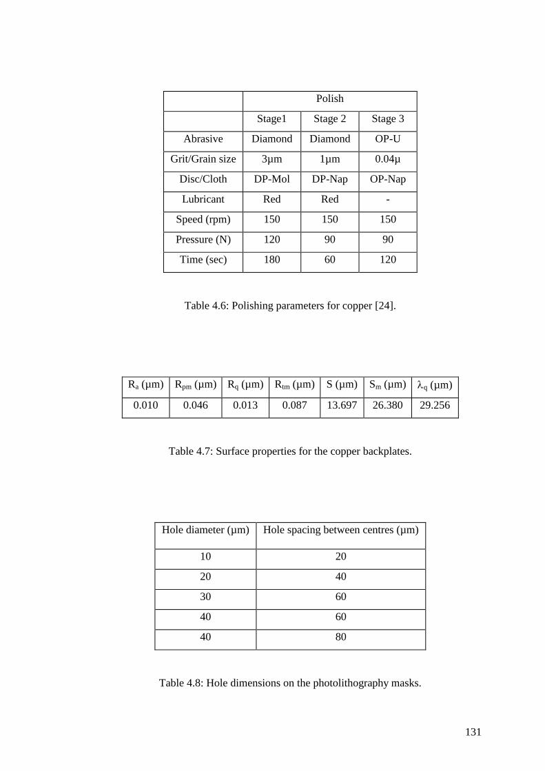
131

Polish

Stage1 Stage 2 Stage 3

Abrasive Diamond Diamond OP-U

Grit/Grain size 3µm 1µm 0.04µ

Disc/Cloth DP-Mol DP-Nap OP-Nap

Lubricant Red Red -

Speed (rpm) 150 150 150

Pressure (N) 120 90 90

Time (sec) 180 60 120

Table 4.6: Polishing parameters for copper [24].

Ra (µm) Rpm (µm) Rq (µm) Rtm (µm) S (µm) Sm (µm) q (µm)

0.010 0.046 0.013 0.087 13.697 26.380 29.256

Table 4.7: Surface properties for the copper backplates.

Hole diameter (µm) Hole spacing between centres (µm)

10 20

20 40

30 60

40 60

40 80

Table 4.8: Hole dimensions on the photolithography masks.

132

The copper backplates were then etched in a solution of 50g ammonium

persulphate in 350ml of water, maintained at 50°C in a heated water bath. In order to

determine the etch rate of the copper bar used, a piece of the original bar was

progressively immersed in the etchant for periods of 2 minutes, and then measured on

the Taylor-Hobson Form Talysurf. From these measurements it was calculated that the

etch rate was 4-5µm/minute. The range of backplate hole sizes was intended to show

what effect the hole diameter and spacing would have on the frequency response of

each device, as the depth would be kept constant. In order to investigate the effect of

hole depth, two backplates with the same hole spacing but different hole diameters

(30x60 and 40x60) were etched for different lengths of time until the holes were

approximately the same diameter, but of different depths.

Photographs of the etched backplates are shown in Figures 4.16(a) to (f).

Figure 4.16(a) shows the 30x60 mask after etching and is typical of all the backplates

prepared. The photograph shows the pale area of polished copper beneath the layer of

photoresist, and a regular array of circular features. Each feature consists of a dark

central hole penetrating the layer of photoresist and on into the underlying copper

substrate, surrounded by a pale annulus of undercut mask.

The mask was then removed by washing the backplates in acetone, and then

rinsing firstly with water and finally with methanol before drying with hot air. With

the mask layer removed, the surface of each backplate may now be seen in greater

detail. Figure 4.16(b) shows the 30x60 backplate with the mask removed, with the

other backplates being shown in Figures 16(c) to (f). All the holes are well defined,

with the exception of Figure 4.16(f) for the 10x20 mask which moved during the

etching process due to excessive undercutting, and Figure 4.16(b) for the 30x60 mask.

133

Figure 4.16: Etched backplates (a) with photoresist for the 30x60 mask, and without

photoresist for (b) the 30x60 and (c) the 40x60 mask sizes. Scale 1mm:6.85µm

134

Figure 4.16: Etched backplates with the photoresist removed for (d) the 40x80, (e) the

20x40 and (f) the 10x20 mask sizes. Scale 1mm:6.85µm

135

Mask Mask diameter

(µm)

Mask spacing

(µm)

Etched diameter

(µm)

Etch rate

(µm/min)

10x20 13.8 19.0 N/A N/A

20x40 26.5 39.5 37.4 5.45

30x60 32.3 59.2 47.6 5.10

40x60 46.3 59.2 54.4 4.05

40x80 46.3 81.0 58.5 6.10

Table 4.9: Mask and hole dimensions for each of the copper backplates.

This backplate was etched for a longer time to try and obtain two backplates with

holes of identical diameter and spacing, but different hole depths. The hole edges are

therefore slightly rougher, as the etchant has had longer to remove copper along the

crystal boundaries. The diameters of the holes were measured from the photographs in

Figures 4.16 and are shown in Table 4.9 for the various masks.

It is evident from the dimensions shown in Table 4.9 that the hole diameters in

the deposited layer of photoresist are different to those on the photolithography mask,

whereas the hole spacing is virtually identical. This was due to the ultraviolet light

diffusing around the edges of the photoresist layer and blurring the feature edges. In

addition, the ultraviolet light source was not uniform in intensity, and the masks were

probably slightly overexposed in some areas.

The depths of the holes were then measured using the Taylor-Hobson Talysurf.

Figure 4.17 shows typical surface profiles obtained for (a) a 1mm section of the

backplate and (b) an individual hole on the 40x80 backplate, and similar results were

obtained for all backplates. No discernible regular structure could be determined for

the 10x20 backplate and so this was not used in the experiments. Measuring the depth

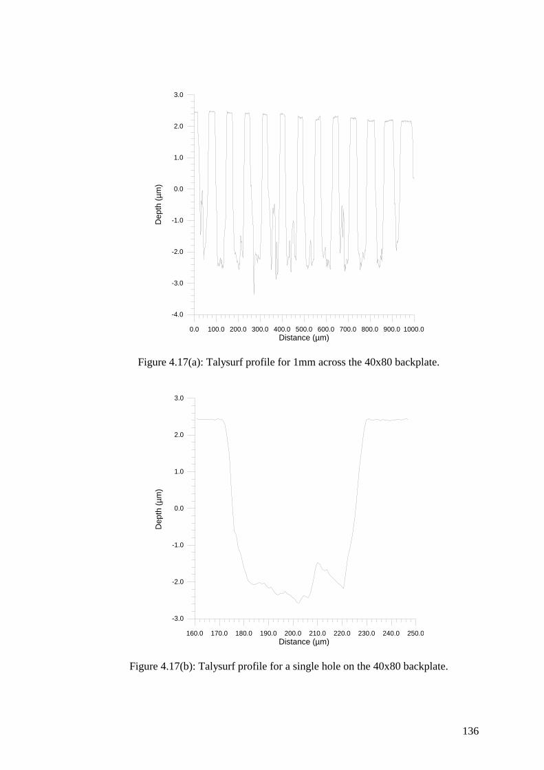
136

0.0 100.0 200.0 300.0 400.0 500.0 600.0 700.0 800.0 900.0 1000.0

Distance (µm)

-4.0

-3.0

-2.0

-1.0

0.0

1.0

2.0

3.0

De

pth

(µ

m)

Figure 4.17(a): Talysurf profile for 1mm across the 40x80 backplate.

160.0 170.0 180.0 190.0 200.0 210.0 220.0 230.0 240.0 250.0

Distance (µm)

-3.0

-2.0

-1.0

0.0

1.0

2.0

3.0

De

pth

(µ

m)

Figure 4.17(b): Talysurf profile for a single hole on the 40x80 backplate.

137

Device 20x40 30x60 40x60 40x80 Flat

hole diameter (µm) 37.4 47.6 54.4 58.5 -

hole area (µm2) 1096.8 1779.5 2324.3 2687.8 -

hole spacing (µm) 39.5 59.2 59.2 81.0 -

hole depth (µm) 4.4 6.2 4.6 4.7 -

hole volume (µm3) 4833.8 11032.9 10691.8 12632.7 -

minimum spacing (µm) 2.1 11.6 4.8 22.5 -

area ratio 0.70 0.51 0.66 0.41 -

spacing ratio 0.95 0.80 0.91 0.72 -

total flat area (mm2) 52.68 37.99 49.62 30.65 74.82

total hole volume (mm3) 0.09742 0.2283 0.1159 0.2076 0.0

Table 4.10: Backplate surface parameters.

of the holes in each backplate was not straightforward, as there was no guarantee that

the stylus on the Talysurf was travelling down the centre line of a row of holes, and so

the dimensions obtained must be treated with caution.

4.3.1 Experimental technique

A transducer was manufactured from each of the etched copper backplates and

a 6µm Mylar film. Each transducer was then in turn used as a receiver of ultrasound

generated by the silicon backplate device as described in the previous section on brass

backplate transducers. 100V of d.c. bias was applied to each transducer via the

Cooknell amplifier, and the air gap between source and receiver was 20mm.

138

In an attempt to find the connection (if any) between the frequency response

and sensitivity of the devices, and the dimensions of the features of the backplates, the

following properties were considered: hole diameter, hole depth, hole spacing, hole

volume, minimum spacing, hole area, area ratio (hole area/hole spacing squared),

spacing ratio (diameter/spacing), and the total flat area of the device. The values used

are shown in Table 4.10.

4.3.2 The effects of the hole dimensions

The frequency spectra for each of the backplates are shown in Figure 4.18(a)

showing their relative sensitivity and (b) normalised to the maximum amplitude in

each FFT to show their relative bandwidth. The relationship between 3dB bandwidth

and sensitivity is shown in Figure 4.19, and as before there is a trade off between the

two. However, there were no conclusive trends visible between the various backplate

parameters shown in Table 4.10, and absolute sensitivity and bandwidth for each

transducer, although it is possible that there is a relationship between the hole volume

and the response of the devices. A statistical analysis of a larger number of backplates

is needed to verify this. There was, however, an increase in sensitivity for all the

etched devices over the flat unetched backplate, so the holes are having some effect.

More air has been introduced between the backplate and the polymer film by the

holes, making the film less rigid. It was thought that there may have been a connection

between hole spacing (or minimum distance between hole edges), hole diameter and

hole depth, as these properties may be likened to the rail width, groove width and

groove depth of grooved backplates. Such a connection has been seen in previous

work by Suzuki et al. [21].

139

0.0 0.2 0.4 0.6 0.8 1.0 1.2 1.4 1.6 1.8 2.0

Frequency (MHz)

0.0

10.0

20.0

30.0

40.0

50.0

60.0

Se

nsitiv

ity (

arb

itra

ry u

nits)

FLAT

40X80

40x60

30x60

20x40

Figure 4.18(a): Frequency spectra for all the copper backplates, showing their relative

sensitivity.

0.0 0.2 0.4 0.6 0.8 1.0 1.2 1.4 1.6 1.8 2.0

Frequency (MHz)

0.0

0.1

0.2

0.3

0.4

0.5

0.6

0.7

0.8

0.9

1.0

No

rmalis

ed

se

nsitiv

ity

FLAT

40x80

40x60

30x60

20x40

Figure 4.18(b): Normalised frequency spectra for all the copper backplates, showing

their relative bandwidth.

140

30.0 35.0 40.0 45.0 50.0 55.0 60.0

Relative sensitivity (arbitrary units)

0.0

0.1

0.2

0.3

0.4

0.5

0.6

3d

B b

an

dw

idth

(M

Hz)

20x40

30x60

40x60

40x80

FLAT

Figure 4.19: Plot of sensitivity against bandwidth for the copper backplates.

4.4 Discussion

The subject of capacitance air-coupled transducers is attracting much interest

as there is yet to be found a definitive model for the devices. The work described here

compliments previous work on random backplate transducers [17], and has shown

that there appears to be an optimum bias voltage for the frequency response of the

device, and the film thickness used.

However, there also appeared to be an optimum bias voltage to maximise the

sensitivity of the device, which is different to that required for maximum bandwidth.

As the film is pulled more firmly onto the backplate at higher bias voltages, the film

becomes more heavily damped and so the bandwidth increases. The air behind the

membrane is compressed or squeezed out completely, so that the film conforms more

141

precisely to the backplate surface profile. Where films of different thickness were

used on the same backplate, and with the same bias voltage applied, there appeared to

be an optimum thickness of film, below which there was no gain in sensitivity. It is

possible that the film thickness also needs to be matched to the surface properties of

the backplate, but due to the small number of backplates and films used in this study,

further work is needed for confirmation of this.

It was noted that the shape of the frequency spectrum also changed with

increasing bias voltage, and that the profile was made up from two distinct portions,

the first possibly being determined by the film thickness, and the second by the

backplate surface. It was not possible to calculate the theoretical frequencies for the

membrane alone, as its stiffness was not known and could not easily be measured. It

would be reasonable to assume that the stiffness of the film is related to the bias

voltage applied, and that equation {4.2} could be adapted to account for this in future

work.

From the data shown in Table 4.5, it would appear that there was little

agreement between theory and experiment when using surface roughness parameters

as an approximation to the air gap. However the linear relationship to the inverse

square root seen in previous work [17] could be observed in Figures 4.7 and 4.10, and

so it is possible that equation {4.1} needs to be modified to apply to broadband

devices. It was also noted that results improved slightly when thinner films were used,

possibly due to the film conforming more accurately to the surface profile of the

backplate. The long term suitability of brass as the backplate material is probably not

ideal, as the surface tarnishes with time, and so the surface properties of the

backplates may change after the transducers have been assembled. Stainless steel may

be more suitable.

142

The work on chemically etched backplates showed that in this study, there was

no conclusive link between the hole dimensions and the response of the devices for

the 6µm membrane thickness and 100V bias used, although a possible relationship

with hole volume may have existed. Links between the hole dimensions and the

frequency response of capacitance devices have, however, been observed by other

authors [21] who worked with silicon. The use of chemical etching to consistently

produce identical metallic backplates is difficult, as so many variables need to be

removed. It was apparent that fresh chemicals were necessary for each backplate, or

some other compensation for the loss in etchant strength between successive devices.

The isotropic etch also caused problems, as it was difficult to produce holes of the

same diameter but different depths. The anisotropic properties of silicon have been

exploited by other authors [20-22] for this purpose, but silicon requires the use of

hydrofluoric acid (HF) as an etchant which is far from ideal. Other processes such as

ion beam machining or laser machining may produce more consistent results.

However, a comprehensive study of this would probably fill several other Ph.D.

theses, and so can only be speculated about here.

4.5 Conclusions

A series of capacitance air-coupled transducers with roughened and polished

brass backplates were made, and the effects of changing the roughness of the surface

were investigated. A linear relationship between sensitivity and bandwidth was

observed, and the frequency response was inversely proportional to the square root of

the surface roughness of the backplate, as seen in previous work on the same subject.

Changing the thickness of the polymer film showed a similar relationship with the

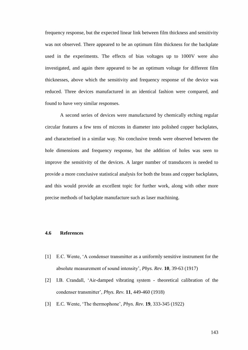
143

frequency response, but the expected linear link between film thickness and sensitivity

was not observed. There appeared to be an optimum film thickness for the backplate

used in the experiments. The effects of bias voltages up to 1000V were also

investigated, and again there appeared to be an optimum voltage for different film

thicknesses, above which the sensitivity and frequency response of the device was

reduced. Three devices manufactured in an identical fashion were compared, and

found to have very similar responses.

A second series of devices were manufactured by chemically etching regular

circular features a few tens of microns in diameter into polished copper backplates,

and characterised in a similar way. No conclusive trends were observed between the

hole dimensions and frequency response, but the addition of holes was seen to

improve the sensitivity of the devices. A larger number of transducers is needed to

provide a more conclusive statistical analysis for both the brass and copper backplates,

and this would provide an excellent topic for further work, along with other more

precise methods of backplate manufacture such as laser machining.

4.6 References

[1] E.C. Wente, ‘A condenser transmitter as a uniformly sensitive instrument for the

absolute measurement of sound intensity’, Phys. Rev. 10, 39-63 (1917)

[2] I.B. Crandall, ‘Air-damped vibrating system - theoretical calibration of the

condenser transmitter’, Phys. Rev. 11, 449-460 (1918)

[3] E.C. Wente, ‘The thermophone’, Phys. Rev. 19, 333-345 (1922)

144

[4] E.C. Wente, ‘Sensitivity and precision of the electrostatic transmitter for

measuring sound intensities’, Phys. Rev. 19, 498-503 (1922)

[5]

Brüel and Kjær, Master Catalogue - Electronic Instruments, (K. Larsen & Sons,

Denmark, 1989)

[6] G.S.K. Wong and A.F.W. Embleton (eds.), AIP Handbook of condenser

microphones - Theory, calibration and measurements, (AIP Press, New York,

1995)

[7] N.W. McLachlan, Loudspeakers, (Clarendon Press, Oxford, 1934)

[8]

W. Kuhl, G.R. Schodder and F.-K. Schröder, 'Condenser transmitters and

microphones with solid dielectric for airborne ultrasonics', Acustica 4, 519-532

(1954)

[9] K. Matsuzawa, ‘Condenser microphones with plastic diaphragms for airborne

ultrasonics I’, J. Phys. Soc. Japan 13, 1533-1543 (1958)

[10] K. Matsuzawa, ‘Condenser microphones with plastic diaphragms for airborne

ultrasonics II’, J. Phys. Soc. Japan 15, 167-174 (1960)

[11] M. Rafiq and C. Wykes, 'The performance of capacitive ultrasonic transducers

using v-grooved backplates', Meas. Sci. Technol. 2, 168-174 (1991)

[12]

J. Hietanen, P. Mattila, J. Stor-Pellinen, F. Tsuzuki, H. Väätäjä, K. Sasaki and

M. Luukkala, 'Factors affecting the sensitivity of electrostatic ultrasonic

transducers', Meas. Sci. Technol. 4, 1138-1142 (1993)

[13]

J. Hietanen, J. Ignatius and J. Stor-Pellinen, ‘Electrostatic solutions for a

capacitive ultrasonic air transducer with a uniformly V-grooved backplate’,

Sensors and Actuators A 45, 95-98 (1994)

[14] P. Mattila and J. Hietanen, ‘Bandwidth control of an electrostatic ultrasonic

transducer’, Sensors and Actuators A 45, 203-208 (1994)

145

[15]

W.S.H. Munro and C. Wykes, ‘Arrays for airborne 100kHz ultrasound’,

Ultrasonics 32, 57-64 (1994)

[16] W.S.H. Munro, S. Pomeroy, M. Rafiq, H.R. Williams, M.D. Wybrow and C.

Wykes, ‘Ultrasonic vehicle guidance transducer’, Ultrasonics 28, 350-354

(1990)

[17] H. Carr and C. Wykes, 'Diagnostic measurements in capacitive transducers',

Ultrasonics 31, 13-20 (1993)

[18]

M.J. Anderson, J.A. Hill, C.M. Fortunko, N.S. Dogan and R.D. Moore,

‘Broadband electrostatic transducers: Modeling and experiments’, J. Acoust.

Soc. Am. 97, 262-272 (1995)

[19]

W. Kühnel and G. Hess, 'A silicon condenser microphone with structured

backplate and silicon nitride membrane', Sensors and Actuators A 30, 251-258

(1992)

[20]

D.W. Schindel, D.A. Hutchins, L. Zou and M. Sayer, ‘The design and

characterization of micromachined air-coupled capacitance transducers’, IEEE


[21]

K. Suzuki, K. Higuchi and H. Tanigawa, 'A silicon electrostatic ultrasonic

transducer', IEEE Trans. Ultrason. Ferroelec. Frequ. Contr. UFFC 36, 620-627

(1989)

[22] M.I. Haller and B.K. Khuri-Yakub, 'A surface micromachined electrostatic

ultrasonic air transducer', IEEE Ultrason. Symp. 1994 (Cannes), 1241-1244

[23] J. Hietanen, J. Stor-Pellinen, M. Luukkala, P. Mattila, F. Tsuzuki and K. Sasaki,

'A Helmholtz resonator model for an electrostatic ultrasonic air transducer with a

V-grooved backplate', Sensors and Actuators A 39, 129-132 (1993)

146

[24] R. Høeg and E. Weidmann, Metallographic sample preparation - How to select

proper grinding and polishing procedures, (Struers Personal Metalog, 1992)

Chapter 5: Thickness estimation using air-coupled Lamb waves

147

5.1 Introduction

This chapter describes how air-coupled plate waves (Lamb waves) may be used to

estimate the thickness of thin plates of material. An overview of Lamb wave theory will be

given, followed by a description of two methods by which the plate thickness may be

found. A series of experiments is then described which use laser-generated Lamb waves

and an air-coupled capacitance receiver to reconstruct the velocity dispersion curves.

These are then compared to theoretical curves calculated using a FORTRAN program, and

the thickness of the plate is estimated. The final part of the work will investigate the use of

another air-coupled capacitance transducer to replace the laser source.

5.1.2 A brief history of Lamb waves

Plate waves or Lamb waves occur in a thin sample of material, where the two free

boundaries of a plate parallel to the direction of wave motion are close enough to prevent

the propagation of pure surface waves and bulk modes. The initial theory was devised by

Lamb [1] in 1917, but the equations were not fully explained and only a limited number of

solutions were presented. A more comprehensive set of solutions was not produced until

1950 by Mindlin [2], who showed the results for both real and imaginary wave numbers.

Later works by Viktorov [3] and then Achenbach [4] cover the equations and general

theory in greater detail. However, the results for even the simplest geometry in isotropic

materials are still sufficiently complex to generate recent interest in the theory [5-7] or

other approximations to the dispersion relations [8,9]. An overview of some of the more

relevant parts of the theory will be given in the next section.

148

With the advent of more complicated engineering materials and techniques,

interest in both the theory and practical applications of Lamb waves has increased,

particularly in the examination of adhesive bonds [10-12] and anisotropic or composite

materials [13-22]. Some of the experimental work has been carried out using standard

direct coupling techniques [15,16], but most used some form of immersion tank [18-20],

relying on the fact that Lamb waves ‘leak’ or re-radiate back into the surrounding medium,

a phenomena which has been visualised using Schlieren optics [23,24]. Earlier work by

Merkulov [25] showed that provided the density of the plate was much greater than that of

the surrounding medium, damping effects were negligible. For some modern composite

materials this is no longer the case.

By removing the coupling medium altogether, any possible damping effects are

negated. This has been achieved to date by the used of entirely laser based non-contact

techniques, using pulsed lasers for ultrasonic generation, and interferometers or some

form of beam deflection device as the detector [26-32]. Some work has also been done

using electromagnetic acoustic transducers (EMATs) [33]. However, these techniques

have the usual associated drawbacks, namely the cost, fragility and surface requirements of

most interferometers, and the restriction of only electrically conducting samples for

EMATs.

An alternative method is to use air as the coupling medium, a method already used

to study the mechanical properties of paper [34,35]. With the recent advances in

air-coupled capacitance transducer technology [36,37], giving improved sensitivity and

bandwidth, a further investigation into this technique was undertaken. The work to be

presented in this chapter will describe how air-coupled Lamb waves were successfully

used to evaluate a variety of materials.

149

5.2 An overview of Lamb wave theory

As mentioned in previous chapters, Lamb waves [3,4] or plate waves occur in thin

samples of material, where the two boundaries of the plate parallel to the direction of wave

motion are close enough to prevent propagation of pure surface waves and bulk modes.

Lamb waves are dispersive, i.e. waves with different frequencies travel at different

velocities in the same material, and so the well known relation:

fc

{5.1}

still applies, but here c is no longer a constant, rather a function of the wavelength. Lamb

waves may be classified into two groups depending on their mode of vibration.

Asymmetric or ‘a’ modes occur when the motion of the plate surfaces is asymmetrical

about a line through the centre of the sample in the direction of propagation, as shown

schematically in Figure 5.1(a). Symmetric or ‘s’ modes occur when the motion of the plate

surfaces is symmetric about this line, as shown schematically in Figure 5.1(b).

The fundamental characteristic of a Lamb wave is its phase velocity cp, which is a

function of the frequency of the wave and the thickness of the plate. This differs from the

velocity of energy propagation, or group velocity cg, although this is also frequency

dependent. Referring to Figure 5.2, the interference of two or more carrier waves of

slightly different frequencies f1 and f2, travelling at their respective phase velocities cp1 and

cp2, form a modulation or group of waves of frequency fg travelling with a group velocity

of cg. The group velocity may be determined using:

cd

dkg

{5.2}

where k is the wave number.

150

Figure 5.1: Plate surface motion for (a) asymmetric and (b) symmetric Lamb waves.

f1

f2

fg

Figure 5.2: The interference of two waves of slightly different frequencies f1 and f2,

travelling at phase velocities cp1 and cp2, to produce a modulation of frequency fg travelling

at a group velocity cg.

151

The phase velocity may be found using the Rayleigh-Lamb frequency relations.

For the symmetric ‘s’ modes:

( - . )

( - . ) = -

( - ) ( - )

( - )

tan

tan

1 4 1

2 1

2

2 2

2 2 2 2

2 2

a d

b a d

a a b a

a {5.3}

and for the asymmetric ‘a’ modes:

( - . )

( - . ) = -

( - )

( - ) ( - )

tan

tan

1 2 1

4 1

2

2 2

2 2

2 2 2 2

a d

b a d

a

a a b a {5.4}

where:

= = =. .

ac

cb

c

cd

f t

c

t

p

t

L t

{5.5}

with ct and cL being the transverse and longitudinal bulk wave velocities in the material, cp

the phase velocity at frequency f, and t the thickness of the plate.

These Rayleigh-Lamb frequency relations have a finite number of real roots, but an

infinite number of imaginary roots and so cannot be solved directly, but rather by

numerical methods. The first root is known as the zero order mode, the next as the first

order, and so on. Figure 5.3 shows a plot of normalised phase velocity (cp/ct) against

frequency-thickness product (f.t) for the first four asymmetric and symmetric modes in

aluminium, with Figure 5.4 showing a similar plot for normalised group velocity (cg/ct)

against frequency-thickness product (f.t). in the same material. It can be seen that apart

from the zero order (a0 and s0) modes, the plots do not extend down to the origin at 0Hz,

and have a cut-off or critical frequency. This is determined by the thickness t of the plate,

and both the longitudinal and transverse wavelengths in the material. For symmetric

modes, critical frequencies occur when:

t etcL L L

2

3

2

5

2, , , . {5.6}

152

0.0 2.0 4.0 6.0 8.0 10.0 12.0 14.0 16.0 18.0 20.0

frequency.thickness product (mm.MHz)

0.0

0.2

0.4

0.6

0.8

1.0

1.2

1.4

1.6

1.8

2.0

No

rma

lise

d p

ha

se

ve

locity c

p/c

t s

0

s1

a0

a1

a2

s2

s3

a3

Figure 5.3: Phase velocity dispersion curves for the first four asymmetric and symmetric

Lamb wave modes in aluminium.

0.0 2.0 4.0 6.0 8.0 10.0 12.0 14.0 16.0 18.0 20.0

frequency.thickness product (mm.MHz)

0.0

0.2

0.4

0.6

0.8

1.0

1.2

1.4

1.6

1.8

No

rma

lised

gro

up

velo

city c

g/ c

t

s0

a0

s1

a1

s2

a2

a3

s3

Figure 5.4: Group velocity dispersion curves for the first four asymmetric and symmetric

Lamb wave modes in aluminium.

153

and:

t etct t t , , , .2 3 {5.7}

Similarly for asymmetric modes:

t etct t t

2

3

2

5

2, , , . {5.8}

and:

t etcL L L , , , .2 3 {5.9}

The total number of modes N in a plate of thickness t at a given frequency f is given by:

Nt t

t L

1

1

2 {5.10}

for the symmetric modes, and by:

Nt t

L t

1

1

2 {5.11}

for the asymmetric modes. In both cases, the expressions in square parentheses are

rounded to the nearest integer.

The cut-off frequencies for symmetric and asymmetric modes higher than zero

order have a physical explanation. The zero order modes are formed by the interaction of

two surface waves, as shown schematically in Figure 5.5(a), and thus exist at all

frequencies in any thickness of plate. As the plate thickness increases (at a given

frequency) or the wavelength decreases (for a given plate thickness), the two surface waves

interact less and less until they become pure surface waves and travel at the Rayleigh wave

velocity, as can be seen from the dispersion curves at high frequency-thickness products.

The higher order modes are formed by the interaction of bulk waves reverberating

in the plate thickness, to form a standing wave or resonance as shown in

154

Figure 5.5: Formation of (a) zero order modes from surface waves, and (b) higher order

modes from standing waves.

Figure 5.5(b). A new mode exists when there is an integral number of half wavelengths

within the plate thickness, for either longitudinal or transverse waves. At lower non-critical

values for a given mode, waves cannot propagate as they are purely imaginary. At higher

non-critical values, the standing wave is no longer travelling perpendicularly to the

surfaces of the plate, and so will propagate with a characteristic phase velocity. The

standing wave is non-dispersive and so has a fixed wavelength S, whereas the Lamb wave

mode will have a varying wavelength L depending on the angle it makes with the plate

surface, and so will exhibit the characteristic dispersion. The actual situation is far more

complex than described here, and a more comprehensive explanation may be found in the

works by Viktorov [3] and Achenbach [4].

155

5.3 Extracting the dispersion relations from Lamb wave data

As can be seen from the Rayleigh-Lamb equations, the velocity (phase or group) of

a Lamb wave is heavily dependent on frequency, plate thickness and bulk wave velocities.

As stated in Chapter 1, the bulk wave velocities are directly related to the elastic properties

(Young’s modulus and Poisson’s ratio) of the material. There are many methods for

extracting the dispersion relations from Lamb wave data, so only the two used in this work

will be described here. The method used by Dewhurst et al. [26] measured the group

velocity using the mean arrival time of a ‘group’ of frequencies, found by inverting the

time between successive maxima in the dispersive a0 mode. A variant of this method,

known as the ‘zero-crossing’ technique, was used in this work and may be explained as

follows. As Lamb waves disperse, waves of different frequencies arrive at different times

due to their varying velocities. For the a0 mode, higher frequencies arrive first, and lower

frequencies later, as both the phase and group velocities increase with frequency, as can be

seen from the dispersion curves in Figures 5.3 and 5.4. For the s0 mode, the low frequency

components arrive first. The zero crossing technique involves measuring the times at

which the waveform crosses the zero amplitude origin, after subtracting any d.c. offset.

Due to the dispersion, a portion of the waveform between successive crossings at, say, t1

and t2 will contain a range of different frequencies, and so may be thought of as a group

with a central frequency f, which corresponds to the inverse of the time difference between

the two crossing times. Provided that the propagation distance x is known, the group

velocity cg at the frequency f may be found using:

( ) = c fx

tg

1

{5.12}

156

The second method used by Hutchins et al. [29] is an extension of the earlier work

by Sachse and Pao [38] for bulk waves, in which the dispersion relation is obtained using

the phase information contained in the fast Fourier transform (FFT) of a Lamb wave

signal, given by:

( ) tan( )

( )( )n

F i

F rn

1

2 2 5.13}

where n is the number of points in the FFT, and F(i) and F(r) are the real and imaginary

parts of the FFT respectively. If the change in phase between successive points of the FFT

is greater than , then discontinuities will occur in the phase spectrum. These may be

corrected by adding to all subsequent points when (i+1) < (i). The total number of

wavelengths n at a certain frequency f between the source and receiver is given by:

n ff

( )

( )

.

2 {5.14}

If the propagation distance x between source and receiver is known, then the wavelength at

the specific frequency f may be found from:

f

x

n f

( ) {5.15}

Then the phase velocity cp will be:

ck

fp

. {5.16}

5.4 Calculation of theoretical curves

The real roots of the Rayleigh-Lamb equations must be found by numerical

methods, the most common being to select a constant frequency f, and then substitute an

increasing value of cp until the equations change sign. The lowest value of cp at which a

157

root occurs will be the zero order mode, the next the first order mode, and so on. A

computer program (see Appendix B) was written in FORTRAN to calculate the dispersion

curves for Lamb waves in isotropic materials. Both phase velocity and group velocity

curves were generated, as the group velocity is simply the differentiation of the phase

velocity curve with respect to frequency, i.e.:

cd

dk kg

{5.17}

c

f f

f

c

f

c

g

2 2

2 2

2 1

2

2

1

1

. . . .

. . . .

{5.18}

= [ - ]

-

cf f

f

c

f

c

g2 1

2

2

1

1

{5.19}

where 1 and 2 denote adjacent points in the frequency spectrum.

Dispersion curves are usually presented as plots of normalised velocity versus

frequency-thickness product (see Figures 5.3 and 5.4), which enable a large number of

plates of different thickness to be represented on one plot. However, a FFT contains

frequency information at discrete intervals, which will be fixed for time domain

waveforms of the same length. Frequency-thickness products for samples of the same

material but different thickness will therefore be difficult to compare with one single

dispersion curve without interpolation. The FORTRAN program used here calculated the

dispersion curves for one specific plate thickness, for any given frequency range at any

frequency interval. This allowed the theoretical curves to be directly compared with

experimentally obtained curves, which would be of velocity versus frequency.

158

5.5 Trial experiments using a contact detector

Experiments were first performed to test the methods of extracting the dispersion

relations from Lamb wave signals. To ensure that sufficient bandwidth was available for

the experiments, a pulsed laser was used to generate signals in thin (<1.0mm) sheets of

various materials, and an electrostatic air-coupled transducer was used as a detector. The

apparatus is shown schematically in Figure 5.6. The laser used was a Lumonics ‘Mini-Q’

q-switched Nd:YAG, operating at a wavelength of 1064nm in the near infra-red, with a

pulse duration of 4ns and maximum pulse energy of 120mJ. The beam was directed onto

the sample using a suitable 45 mirror, and a lens to reduce the 3mm beam diameter to a

point. The air transducer used as a receiver was held in a rotating mount which enabled the

angle between the plate and transducer face to be varied. This altered the range of

frequencies of leaky Lamb waves seen by the detector. The rotary mount was fixed to a

micrometer stage, the motion of which was parallel to the surface of the sample. This

permitted precise changes in the propagation length of the Lamb wave through the sample.

Signals were amplified using a Cooknell CA6/C charge sensitive amplifier, in conjunction

with a SU2/C power supply which enabled a d.c. bias of up to 100V to be applied between

the film and backplate electrodes of the receiver. Waveforms were captured and digitised

on a Tektronix 540 TDS digital oscilloscope, and then transferred via an IEEE-488/GPIB

interface to an IBM PS/2 Model 30 286 computer for storage and later analysis. To ensure

detection of the correct waveform, a contact capacitance device which used the sample as

one electrode as described in previous chapters, was used as a calibrated receiver. This

used the sample as one electrode of a capacitor, and a steel sphere as the other, with a thin

159

Figure 5.6: Schematic diagram of experimental equipment.

polymer dielectric film between them. For more detailed equipment specifications, see

Appendix A.

The first sample to be tested was a 1.2mm thick aluminium sheet. From the

relevant portion of the phase velocity dispersion curves, it can be seen that at frequencies

up to approximately 2MHz in this thickness of plate, the frequency thickness product is

sufficiently low to allow only the two zero order (a0 and s0) modes to exist. A typical Lamb

wave which had propagated through 55mm of the plate is shown in Figure 5.7(a). Both the

s0 and a0 modes are clearly visible, and show the characteristic dispersion. The contact

capacitance transducer is wideband, and has a flat response up to the 10MHz limit of the

charge amplifier. This high bandwidth has allowed some of the higher order modes to be

160

0.0 5.0 10.0 15.0 20.0 25.0 30.0 35.0 40.0 45.0

Time (µs)

-50.0

-40.0

-30.0

-20.0

-10.0

0.0

10.0

20.0

30.0

40.0

Am

plit

ud

e (

mV

)

Figure 5.7(a): Multimode Lamb waves in a 1.2mm aluminium plate, detected using the

contact capacitance device.

0.0 1.0 2.0 3.0 4.0 5.0 6.0 7.0 8.0 9.0 10.0 11.0 12.0

Frequency (MHz)

0.0

0.1

0.2

0.3

0.4

0.5

0.6

0.7

0.8

0.9

1.0

No

rmalis

ed

am

plit

ud

e


161

Theoretical cut off frequency (MHz)

1st order 2nd order 3rd order 4th order 5th order

asymmetric ‘a’ modes 1.30 3.91 5.27 6.52 9.13

symmetric ‘s’ modes 2.61 2.63 5.22 7.83 7.90

Table 5.1: Theoretical cut off frequencies in a 1.2mm thick plate of aluminium.

detected, as at least four other symmetric and four other asymmetric modes will exist at

these values of frequency and thickness. They appear as the high frequency oscillations on

the lower frequency a0 mode, and the non-dispersive vibrations between the s0 and a0

portions of the waveform. A selection of theoretical cut off frequencies up to 10MHz for

asymmetric ‘a’ modes and symmetric ‘s’ modes in a 1.2mm thick plate of aluminium is

shown in Table 5.1, calculated using equations {5.6} to {5.9}, and values of ct=3130ms-1

and cL=6320ms-1

. The FFT of the Lamb wave signal is shown in Figure 5.7(b), where it

can be seen that at least three higher order modes were detected, corresponding to the

peaks beginning at 4.2MHz (possibly the a2 mode), 4.6MHz (a3 or s3 modes) and 9.6MHz

(possibly the a5 mode). The experimental frequencies will not exactly match the theoretical

predictions shown in Table 5.1, as the values of cL and ct used in the calculations will

differ from those in the actual plate.

Using the contact capacitance transducer as a receiver and the laser as a source, the

propagation path of 55mm through the sample was known fairly accurately. The group

velocity of the a0 mode in the 1.2mm aluminium plate is shown in Figure 5.8, where it is

compared with the theoretical curve as calculated by the FORTRAN program using values

162

0.0 0.2 0.4 0.6 0.8 1.0 1.2

Frequency (MHz)

0.0

500.0

1000.0

1500.0

2000.0

2500.0

3000.0

3500.0

Gro

up

ve

locity (

ms -1

)

Theory

Figure 5.8: a0 group velocity in a 1.2mm aluminium plate, found using zero crossing

technique and a contact capacitance transducer - theory vs. experiment.

of 3130ms-1

and 6320ms-1

for the shear and longitudinal velocities respectively. There was

close agreement between the theoretical and experimental results, but there were some

discrepancies. There are several possible sources of error when using this technique, the

most likely being that the method of determining both the frequency of a ‘group’ (inverting

the crossing interval) and the arrival times is inaccurate, the source to receiver distance

may have been inaccurately measured, or that the velocities used to calculate the

theoretical curve were different to the actual velocities in the sample.

Figure 5.9(a) shows the phase information obtained from the FFT of the contact

capacitance transducer waveform. This is the uncorrected phase, and has numerous

discontinuities of which must be removed as described at the end of Section 5.2. The

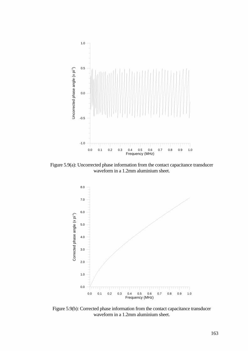
163

0.0 0.1 0.2 0.3 0.4 0.5 0.6 0.7 0.8 0.9 1.0

Frequency (MHz)

-1.0

-0.5

0.0

0.5

1.0

Unco

rre

cte

d p

ha

se a

ng

le (

x p

i-1)

Figure 5.9(a): Uncorrected phase information from the contact capacitance transducer


0.0 0.1 0.2 0.3 0.4 0.5 0.6 0.7 0.8 0.9 1.0

Frequency (MHz)

0.0

1.0

2.0

3.0

4.0

5.0

6.0

7.0

8.0

Co

rre

cte

d p

ha

se

an

gle

(x p

i-1)

Figure 5.9(b): Corrected phase information from the contact capacitance transducer


164

0.0 0.1 0.2 0.3 0.4 0.5 0.6

Frequency (MHz)

0.0

250.0

500.0

750.0

1000.0

1250.0

1500.0

1750.0

2000.0

2250.0

Ph

ase

ve

locity (

ms

-1)

Theory

Figure 5.10: a0 phase velocity in a 1.2mm aluminium plate, found using the FFT phase

reconstruction technique and a contact capacitance transducer - theory vs. experiment.

resulting corrected phase information is shown in Figure 5.9(b). Using the known

propagation path length of 55mm, the reconstructed phase velocity dispersion curve is

shown in Figure 5.10, for the aluminium plate and the contact capacitance transducer. The

experimental data follows the shape of theoretical prediction, but does not agree at high

frequencies. The data is also suspect at very low frequencies because(a) the bandwidth of

the Cooknell amplifier is only well characterised at frequencies in excess of 10kHz, and

(b) the low frequency information contained in the FFT is limited by the length T of the

time domain waveform, i.e.:

=

fT

min

1

2 {5.20}

Similarly, at higher frequencies the information is limited to the upper resolution limit

given by:

165

=

ft

max

1

2 {5.21}

Due to the 10MHZ bandwidth of the amplifier, higher order modes were present,

superimposed over the dispersive a0 signal. Interference between these modes may have

occurred, particularly at the higher a0 frequencies, but the upper frequency limit of the

air-coupled transducer is low enough so that only the zero order modes will be detected.

By using a larger number of points in the time domain waveform so that the accuracy of

this technique improves, the methods described seemed suitable for use with air-coupled

ultrasound for frequencies up to a few hundred kHz .

5.6 Experiments using the air-coupled detector

By replacing the contact capacitance detector with an air-coupled transducer,

similar waveforms were detected in air. Note that the contact device directly measured the

surface displacement caused by the passage of the Lamb wave through the plate, whereas

the air-coupled transducer measures the leaky modes of the Lamb wave. Waves of

different velocity will radiate into air at different angles as dictated by Snell’s law, and so

reception of the symmetric and asymmetric modes will be optimised at different angles.

Figure 5.11 shows a selection of Lamb waves taken at different transducer orientations to

the plate. As expected, the s0 mode (travelling at approximately the longitudinal velocity

cL) was optimised at =2.5, and the a0 mode (travelling at velocities less than the

transverse velocity ct) was optimised at angles of =7 and above. As the s0 mode did not

disperse significantly over this frequency range, it was optimised over only a narrow range

of angles.

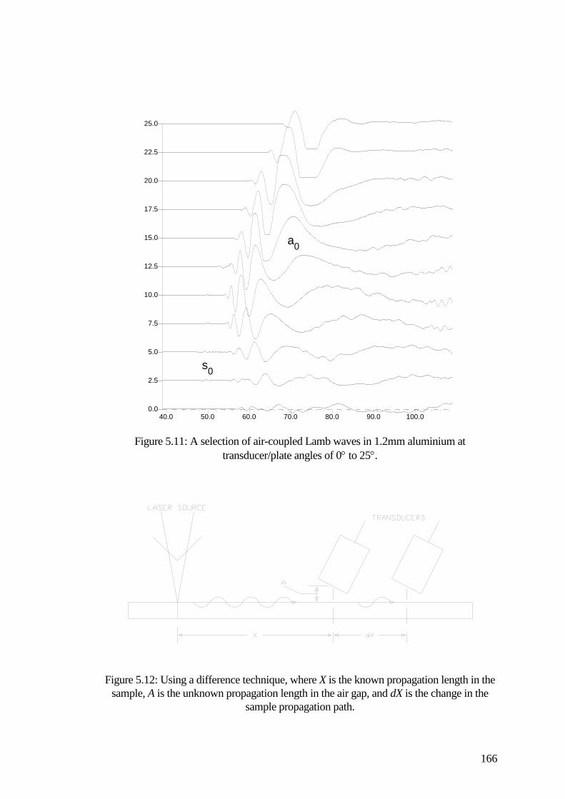
166

40.0 50.0 60.0 70.0 80.0 90.0 100.00.0

2.5

5.0

7.5

10.0

12.5

15.0

17.5

20.0

22.5

25.0

s0

a0

Figure 5.11: A selection of air-coupled Lamb waves in 1.2mm aluminium at

transducer/plate angles of 0 to 25.

Figure 5.12: Using a difference technique, where X is the known propagation length in the

sample, A is the unknown propagation length in the air gap, and dX is the change in the

sample propagation path.

167

Conversely, the highly dispersed a0 mode was optimised over a wide range of

angles (and hence velocities). As the bandwidth of the air transducer was approximately

1.5MHz, only the two zero order modes (a0 and s0) were present in these waveforms. The

amplitude of the a0 mode was much greater than those for the s0 mode, due to the larger

normal motion of the plate caused by propagation of the Lamb wave. As the a0 mode was

present at all angles and gave a larger signal to noise ratio, it was decided to use this mode

for the remainder of the analysis.

The phase and group velocity dispersion curves cannot be determined accurately

from the waveforms shown in Figure 5.11, as the propagation path is not precisely known

due to the air gap. In addition, the air gap will change as the transducer is rotated, and as

the receiver aperture is large (10mm), then this air gap cannot be accurately determined.

There is also an unknown phase delay at the laser source. In order to overcome these

unknowns, a difference technique was employed which is shown schematically in Figure

5.12. The air-coupled receiver was situated some distance X from the laser source, with a

suitable air gap A, and a waveform recorded. The receiver was then moved parallel to the

surface of the plate a known distance dX, so that the perpendicular air gap A was

unchanged, and another waveform recorded. By subtracting the phase and group

information of these two waveforms, the unknown air gap and any phase offset at the

source was eliminated. Thus, any changes were due to the known change in propagation

path in the sample, and the velocities could be calculated with greater accuracy.

5.6.1 Group velocity dispersion curves

The group velocity dispersion curve for the 1.2mm thick aluminium plate as

measured using the difference technique is shown in Figure 5.13, averaged over a range of

168

0.0 0.1 0.2 0.3 0.4 0.5 0.6

Frequency (MHz)

0.0

500.0

1000.0

1500.0

2000.0

2500.0

3000.0

3500.0

Gro

up

ve

locity (

ms

-1)

Theory

Figure 5.13: Group velocity dispersion curve for a 1.2mm aluminium plate, found using


transducer angles. It can be seen that the experimental data follows the theoretical curve

much more closely than the previous results for the same plate using the contact

capacitance transducer, shown earlier in Figure 5.8. The zero crossing method loses

accuracy at higher frequencies, as the digitisation interval of the time domain waveform

begins to limit the precision with which (a) the arrival time and (b) the frequency of each

‘group’ can be determined. Similar results were obtained in a thinner (0.69mm thick)

aluminium plate, where the discrepancies at higher frequencies were larger than for the

thicker sample. At the lower frequency end of the spectrum, the dispersion between

successive zero crossings was greater, and so the assumption used to determine the

frequency of a ‘group’ may not have been valid.

169

0.0 0.1 0.2 0.3 0.4 0.5 0.6

Frequency (MHz)

0.0

250.0

500.0

750.0

1000.0

1250.0

1500.0

1750.0

2000.0

2250.0

Gro

up

ve

locity (

ms

-1)

Theory

Figure 5.14: Group velocity dispersion curve for a 0.85mm brass plate, found using the

zero crossing technique.

0.0 0.1 0.2 0.3 0.4 0.5 0.6

Frequency (MHz)

0.0

500.0

1000.0

1500.0

2000.0

2500.0

3000.0

3500.0

Gro

up

ve

locity (

ms

-1)

Theory

Figure 5.15: Group velocity dispersion curve for a 1.18mm steel plate, found using the

zero crossing technique.

170

The technique was applied to plates of other materials, with curves for 0.85mm

thick brass and 1.18mm thick mild steel being shown in Figures 5.14 and 5.15

respectively. The discrepancies between theory and experiment for brass are attributed to

the values of longitudinal and shear velocity used in the calculations, which are known to

vary widely between different brasses of the same composition, due to the extremely

crystalline structure of the material. By replacing the Nd:YAG laser with a Lumonics

‘Lasermark’ Model 630 CO2 TEA laser, which produced 8J pulses of 100ns duration at

10.6µm in the far infra-red spectrum, a 1.5mm thick sheet of polymethylmethacrylate

(PMMA or perspex) was also be tested with similar results.

5.6.2 Extracting the sheet thickness from the group velocity dispersion curves

The method used by Dewhurst et al. [26] assumed that the plate was thin enough

so that there was little or no dispersion of the zero order symmetric mode. The group

velocity of this s0 mode would then tend towards a single value known as the sheet

velocity, cS. This is in turn related to the square of the group velocity cg of the zero order

asymmetric a0 mode by the expression:

cf t

cg s2 4

3

. . ..

{5.22}

where t is the plate thickness and f = /2. As the s0 mode was not present in the data

obtained, the values of the sheet velocity had to be calculated from the material properties

using the following relation:

cs

4

2

1

2

{5.23}

171

where is the density of the material, and and are the Lamé constants, given by:

=

+

E

2 1 {5.24}

E

3 1 2

2

3 {5.25}

where E is the Young’s modulus and is the Poisson’s ratio of the material. The physical

constants used to calculate the sheet velocities in aluminium, brass and steel are shown in

Table 5.2, with the theoretical sheet velocities cs. By rearranging equation {5.22} to isolate

the thickness, the following expression is obtained:

tc

c

fs

g

3

4

2

. ..

{5.26}

where the term containing cS is the gradient of a graph of cg2 against f that passes through

the origin. Dewhurst et al. [26] used the slope of a best fit line passing through the first

four data points and the origin. For this study, the first linear portion of each plot of cg2 was

used, as shown in Figures 5.16(a) to 5.16(c) for the aluminium, brass and steel sheets

respectively. The estimated sheet thickness of each material, along with the measured

thickness and percentage difference, is shown in Table 5.3.

Material (kg.m-3

) E (x109 Pa) (x10

9 Pa) (x10

9 Pa) cs (ms

-1)

Aluminium 2800 0.34 73.0 27.24 57.88 5429

Brass 8500 0.35 100.0 37.04 86.42 3662

Steel 7860 0.29 210.0 81.40 16.67 5646

Table 5.2: Physical constants and the calculated sheet velocities cs.

172

0.00 0.05 0.10 0.15 0.20 0.25 0.30

Frequency (MHz)

0.0E+0

1.0E+6

2.0E+6

3.0E+6

4.0E+6

5.0E+6

6.0E+6

7.0E+6

8.0E+6

Gru

op

ve

locity s

qu

are

d (

Cg)2

Experiment

Best fit through origin

Figure 5.16(a): Best fit line through origin and first part of curve for the square of the

group velocity in a 1.2mm aluminium plate. Gradient of best fit is 41.39m2s

-3

0.00 0.05 0.10 0.15 0.20 0.25 0.30

Frequency (MHz)

0.0E+0

5.0E+5

1.0E+6

1.5E+6

2.0E+6

2.5E+6

3.0E+6

Gro

up

ve

locity s

qu

are

d (

Cg)2

Experiment


Figure 5.16(b): Best fit line through origin and first part of curve for the square of the

group velocity in a 0.85mm brass plate. Gradient of best fit is 16.8m2s

-3

173

0.00 0.05 0.10 0.15 0.20 0.25 0.30

Frequency (MHz)

0.0E+0

1.0E+6

2.0E+6

3.0E+6

4.0E+6

5.0E+6

6.0E+6

7.0E+6

Gro

up

ve

locity s

qu

are

d (

Cg)2

Experiment


Figure 5.16(c): Best fit line through origin and first part of curve for the square of the

group velocity in a 1.2mm mild steel plate. Gradient of best fit is 42.33m2s

-3

Estimated thickness (mm) Measured thickness (mm) Difference (%)

Aluminium 1.07 1.20 11%

Brass 0.67 0.85 21%

Steel 1.11 1.18 6%

Table 5.3: Comparison of measured and estimated thickness.

The high difference between estimated and measured thickness for brass (21%) was most

probably due to the use of inaccurate material constants, and hence an incorrect value for

the sheet velocity, cs.

174

5.6.3 Phase velocity dispersion curves

The phase velocity dispersion curve calculated using the FFT reconstruction

technique for a 0.69mm thick aluminium plate is shown in Figure 5.17, and there is

excellent agreement between the experimental and theoretical curves. The low frequency

portion of the experimental curve is suspect, as this phase information when obtained from

the FFT is not real measured data, as the waveforms were padded from 2048 points to

4096 points prior to the FFT. This was to decrease the digitisation interval in the frequency

domain, as the lowest measurable frequency is determined by the total length of the time

domain waveform, as mentioned previously in equation {5.20}. By padding the waveform

with zeros to increase T before the FFT to increase the frequency resolution, additional

errors are introduced, as the true signal over this period should contain low frequency

flexural modes which are difficult to compensate for.

Similar results were obtained in steel plates, as shown in Figure 5.18 for a

0.254mm (0.010”) thick shim, although the higher frequency portion of the curve is more

distorted than that for the aluminium. Dispersion curves were also obtained for shims

0.381mm (0.015”), 0.127mm (0.005”), and 0.0762mm (0.003”) thick, with the agreement

between theory and experiment tending to reduce with decreasing thickness. This was due

in part to greater distortion of the shims themselves, and the practical difficulties

encountered when clamping the thinner specimens during the experiments. Note that more

higher frequency information was available in the steel specimens than for the aluminium

plate. Anisotropy may be one other explanation for the increasing errors between theory

and experiment for the thinner steel shims, as they will also become more anisotropic with

reduced thickness due to the rolling processes in their manufacture.

175

0.00 0.05 0.10 0.15 0.20 0.25 0.30 0.35 0.40

Frequency (MHz)

0.0

200.0

400.0

600.0

800.0

1000.0

1200.0

1400.0

1600.0

Ph

ase

ve

locity (

ms

-1)

Theory

Experiment

Figure 5.17: Phase velocity dispersion curve for a 0.69mm aluminium plate, found using

the FFT reconstruction technique.

0.0 0.1 0.2 0.3 0.4 0.5 0.6 0.7 0.8

Frequency (MHz)

0.0

200.0

400.0

600.0

800.0

1000.0

1200.0

1400.0

1600.0

Ph

ase

ve

locity (

ms

-1)

Experiment

Theory

Figure 5.18: Phase velocity dispersion curve for a 0.254mm (0.010”) steel shim, found

using the FFT reconstruction technique.

176

Nominal thickness (mm) Estimated thickness (mm) Percentage difference

0.381 0.38 0.3%

0.254 0.25 1.6%

0.127 0.13 2.4%

0.0762 0.08 5.0%

Table 5.4: Nominal thickness, estimated thickness and percentage difference.

5.6.4 Extracting the sheet thickness from the phase velocity dispersion curves

The earlier work by Hutchins et al. [29] and Oksanen et al. [35] used an

approximation to the dispersion relation to try and obtain the material properties. In this

work to determine the plate thickness, the experimentally obtained phase velocity

dispersion curves were compared directly to the theoretical curves using the well known 2

(chi-squared) numerical fitting between two curves, given by:

2 = D(i) - F(i) 2 {5.27}

where D(i) is the ith data point, and F(i) is the i

th point of the fitting function. A best fit is

achieved when 2 is a minimum. The results for the various steel shims between 0.381mm

(0.015”) and 0.0762mm (0.003”) thick are shown in Table 5.4, with the nominal thickness,

estimated thickness and percentage difference. The discrepancies are less than 5% of the

nominal thickness, and the difference increases with decreasing shim thickness.

Figure 5.19(a) shows a typical air-coupled Lamb wave obtained in a 0.254mm

(0.010”) thick brass plate, and is typical of Lamb waves in various thickness of this

177

150.0 175.0 200.0 225.0 250.0 275.0 300.0 325.0 350.0 375.0

Time (µs)

-60.0

-50.0

-40.0

-30.0

-20.0

-10.0

0.0

10.0

20.0

30.0

Am

plit

ud

e (

mV

)

Figure 5.19(a): A typical Lamb wave in 0.254mm brass shim.

0.00 0.25 0.50 0.75 1.00 1.25 1.50 1.75 2.00 2.25 2.50

Frequency (MHz)

0.0

0.1

0.2

0.3

0.4

0.5

0.6

0.7

0.8

0.9

1.0

No

rmalis

ed

am

plit

ud

e

Figure 5.19(b): The fast Fourier Transform (FFT) of Figure 5.19(a).

178

material. There appears to be some form of modulation in the first part of the signal, caused

by the interference of two waves with similar frequencies. This is further demonstrated by

the FFT of the Lamb wave, shown in Figure 5.19(b), where there are two spectral peaks. It

is possible that the brass was so isotropic that quasi-shear modes were producing two

similar asymmetric modes which were interfering. The theory outlined in this chapter is

restricted to isotropic materials, and so without accurate knowledge of the physical

significance of this phenomenon, further experiments in brass shim were not performed.

5.7 Entirely air-coupled experiments

A second set of experiments was performed, using the apparatus shown

schematically in Figure 5.20, where the pulsed laser source had been replaced by a second

air transducer, so that the entire system was air-coupled. The source was driven using a

Panametrics pulser/receiver model 5055PR, which generated transient voltages of

approximately -200V. Both the source and receiver were orientated at the same angle to

the plate, and offset to allow the Lamb waves to propagate in the sample before being

detected. The difference technique employed with the laser source was again used here.

The phase velocity dispersion curve for a 0.69mm aluminium plate is shown in

Figure 5.21, and there is reasonable agreement between 0.1 and 0.25MHz. Similar results

were obtained in 0.381mm (0.015”) and 0.254mm (0.010”) thick steel shims.

Discrepancies between the theoretical curves and the experimental data are more

prominent than for the laser source, because of practical problems aligning both the source

and receiver transducers with the plate, and the reduced bandwidth and energy of the

source, as all three curves appear to agree best with the theoretical predictions over the

same frequency range.

179

Figure 5.20: Schematic diagram of apparatus for entirely air-coupled testing using Lamb

waves.

0.00 0.05 0.10 0.15 0.20 0.25 0.30 0.35 0.40

Frequency (MHz)

0.0

200.0

400.0

600.0

800.0

1000.0

1200.0

1400.0

1600.0

1800.0

Ph

ase

ve

locity (

ms

-1)

Theory

Experiment

Figure 5.21: Phase velocity dispersion curve for a 0.69mm aluminium plate, obtained

using air-coupled source and receiver.

180

5.8 Discussion

The two methods of Lamb wave analysis used in this chapter have different

requirements when collecting the experimental data. The zero crossing technique requires

as small a time sampling interval as possible, so that each crossing point may be precisely

determined. For the FFT phase reconstruction technique, a long total time is needed to

ensure both accurate low frequency sampling, and that the change in phase between

successive points in the FFT is less than radians. This means that either a large number

of data points or a long sampling interval is needed. In practice, a compromise between the

two had to be used, due to the physical limitations of the oscilloscope and the memory

available on the PC used for analysis.

It would seem from the limited success of the air transducer as a source that there

was insufficient bandwidth and signal energy to investigate metal shims using an entirely

air-coupled system. Both transducers need to be inclined at the correct angle for maximum

energy transfer, and the range of frequencies which leak into air at that angle will also be

limited. Using a laser source increased the bandwidth of the Lamb wave generated in the

shims, and hence the accuracy of the results. The pulsed laser may not be practical for use

on thin polymer films, though, as localised melting of the sample would probably occur,

and so the entirely air-coupled technique may have more success with polymer and

composite materials, particularly as the impedance mismatch between the sample and air

would be reduced. This would be an ideal subject for further investigation.

The zero crossing technique, while simple and quick to implement, has several

possible sources of error. The sheet velocity in the material must be known to determine

the plate thickness, and to avoid using material constants obtained from the literature, this

must be measured experimentally using the s0 mode. However, the s0 mode only

181

approaches the sheet velocity when the sample is extremely thin, or when the wavelength

is very small (i.e.: at high frequencies). The angles at which the s0 and a0 modes leak into

the surrounding air are different, and so the air transducer may only be optimised for one

of them at a time.

The FFT phase reconstruction technique would appear to be more accurate,

although computationally laborious as the comparison of the theoretical and experimental

curves using the 2 technique requires the calculation of multiple curves for samples of

different thickness and frequency ranges. A single curve of frequency-thickness product

could be used, but the theoretical and experimental points would not necessarily coincide,

and so some form of interpolation would be required and thus introduce further errors. As

with the zero crossing technique, the bulk wave velocities must be known in the material

to determine the plate thickness, and the values in thin rolled shims may differ widely from

the theoretical values, or those obtained from thicker samples. The FFT phase

reconstruction technique has the advantage that it may be used for any Lamb mode in any

thickness of plate, provided that the individual modes can be isolated. In addition, the

technique may be used to evaluate both phase and group velocity dispersion, as the group

velocity curve may be found by a simple differentiation of the phase dispersion curve.

5.9 Conclusions

Two techniques have been used to estimate the thickness of thin metal plates using

non-contact leaky Lamb waves. Using a pulsed laser source and a micromachined

air-coupled capacitance transducer as a receiver, a difference technique was employed to

overcome the unknown delays of the air gap between plate and receiver. The thickness

was estimated by comparing the zero order mode velocity dispersion curves to theoretical

182

predictions calculated by a FORTRAN program. The first experimental technique

determined the group velocity dispersion curves using a zero crossing method, and the

thickness of aluminium and steel plates 1.2mm thick was estimated to within 11%, and a

brass plate to within 21%. The second technique reconstructed the phase velocity

dispersion curves from the FFT of a Lamb wave, and the thickness of steel shims between

0.07mm and 0.4mm thick were estimated to within 5%.

Limited success was achieved using an air-transducer as the ultrasonic source due

to the reduced bandwidth, although this technique shows promise for future work with

broadband transducers. The techniques shown here may be used to test any isotropic

sample, and could also be applied to anisotropic materials such as fibre reinforced

composites if the theoretical dispersion curves can be calculated.

5.10 References

[1] H. Lamb, ‘On waves in an elastic plate’, Proc. Royal Society London, Series A, 93,

114-128 (1917)

[2] R.D. Mindlin, ‘Waves and vibrations in isotropic elastic plates’, in Structural

Mechanics, J.N. Goodier and N.J. Hoff (eds.), (Pergamon, New York, 1950)

[3] I.A. Viktorov, ‘Rayleigh and Lamb waves - Physical Theory and Applications’,

Plenum Press, New York (1967)

[4] J.D. Achenbach, ‘Wave Propagation in Elastic Solids’, Elsevier Science Publishers,

Netherlands (1990)

[5] J. Wolf, T.D.K. Ngoc, R. Kille and W.G. Mayer, ‘Investigation of Lamb waves

having a negative group velocity’, J. Acoust. Soc. Am. 83, 122-126 (1988)

183

[6] Q. Zhu and W.G. Mayer, ‘On the crossing points of Lamb wave velocity dispersion

curves’, J. Acoust. Soc. Am. 93, 1893-1895 (1993)

[7] D.S. Chandrasekharaiah, ‘Rayleigh-Lamb waves in an elastic plate with voids’, J.

Appl. Mech. 54, 509-512 (1987)

[8] W. Maysenhölder, ‘Analytical determination of the group velocity of an arbitrary

Lamb wave from its phase velocity’, Acustica 77, 208 (1992)

[9] J. Kaplunov, J. Nolde and N. Veksler, ‘Determination of parameters of elastic layer

by measured dispersion curves of zero-order Lamb-type waves’, Proc. Estonian

Acad. Sci. Phys. Math. 41, 39-48 (1992)

[10] A.K. Mal, P.-C. Xu and Y. Bar-Cohen, ‘Analysis of leaky Lamb waves in bonded

plates’, Int. J. Eng. Sci. 27, 779-791 (1989)

[11] M.R. Karim and A.K. Mal, ‘Inversion of leaky Lamb wave data by simplex

algorithm’, J. Acoust. Soc. Am. 88, 482-491 (1990)

[12] R.Y. Vasudeva and P.G. Rao, ‘Influence of voids in interface zones on Lamb wave

propagation in composite plates’, J. Acoust. Soc. Am. 89, 516-522 (1991)

[13] D.E. Chimenti and A.H. Nayfeh, ‘Leaky Lamb waves in fibrous composite

laminates’, J. Appl. Phys. 58, 4531-4538 (1985)

[14] A.N. Podlipenets and N.A. Shulga, ‘Numerical study of the propagation of Rayleigh

and Lamb waves in orthotropic periodic structures’, Soviet Applied Mechanics 23,

1013-1017 (1987)

[15] B. Tang and E.G. Henneke II, ‘Lamb-wave monitoring of axial stiffness reduction of

laminated composite plates’, Mat. Eval. 47, 928-934 (1988)

[16] D. Noiret and J. Roget, ‘Calculation of wave propagation in composite materials

using the Lamb wave concept’, Journal of Composite Materials 23, 195-206 (1989)

184

[17] G.R. Liu, J. Tani, K. Watanabe and T. Ohyoshi, ‘Lamb wave propagation in

anisotropic laminates’, J. Appl. Mech. 57, 923-929 (1990)

[18] V. Dayal and V.K. Kinra, ‘Leaky Lamb waves in an anisotropic plate. I: An exact

solution and experiments’, J. Acoust. Soc. Am. 85, 2268-2276 (1989)

[19] D.E. Chimenti and R.W. Martin, ‘Nondestructive evaluation of composite laminates

by leaky Lamb waves’, Ultrasonics 29, 13-21 (1991)

[20] V. Dayal and V.K. Kinra, ‘Leaky Lamb waves in an anisotropic plate. II:

Nondestructive evaluation of matrix cracks in fiber-reinforced composites’, J.

Acoust. Soc. Am. 89, 1590-1598 (1991)

[21] W. Lin and L.M. Keer, ‘A study of Lamb waves in anisotropic plates’, J. Acoust.

Soc. Am. 92, 888-894 (1992)

[22] T. Kundu and B. Maxfield, ‘A new technique for measuring Rayleigh and Lamb

wave speeds’, J. Acoust. Soc. Am. 93, 3066-3073 (1993)

[23] L.R. Dragonette, ‘Schlieren visualization of radiation caused by illumination of

plates with short acoustical pulses’, J. Acoust. Soc. Am. 51, 920 (1972)

[24] J.-F. Piet, G. Quentin, M. de Billy, Q.-G Zhu and W.G. Mayer, ‘Phase of Lamb

wave radiation from a plate immersed in a liquid’, Ultrasonics 30, 297-300 (1992)

[25] L.G. Merkulov, ‘Damping of normal modes of a plate immersed in a liquid’, Sov.

Phys. Acoust. 10, (1964)

[26] R.J. Dewhurst, C. Edwards, A.D.W. McKie and S.B. Palmer, ‘Estimation of the

thickness of thin metal sheet using laser generated ultrasound’, Appl. Phys. Lett. 51,

1066-1068 (1987)

[27] D.A. Hutchins, K. Lundgren and S.B. Palmer, ‘A laser study of transient Lamb

waves in thin materials’, J. Acoust. Soc. Am. 85, 1441-1448 (1989)

185

[28] H. Nakano and S. Nagai, ‘Laser generation of antisymmetric Lamb waves in thin

plates’, Ultrasonics 29, 230-234 (1991)

[29] S.E. Bobbin, J.W. Wagner and R.C. Cammerata, ‘Determination of the flexural

modulus of thin films from measurement of the first arrival of the symmetric Lamb

wave’, Appl. Phys. Lett. 59, 1544-1546 (1991)

[30] S.E. Bobbin, J.W. Wagner and R.C. Cammerata, ‘Interpretation of laser-generated

low-order Lamb waves for elastic modulus measurements in thin films’, Ultrasonics

30, 87-90 (1992)

[31] N.A. Schumacher, C.P. Burger and P.H. Gien, ‘A laser-based investigation of

higher-order modes in transient Lamb waves’, J. Acoust. Soc. Am. 93, 2981-2984

(1993)

[32] H.I. Ringermacher, F.A. Reed and J.R. Strife, ‘Laser ultrasonics for coating

thickness evaluation at 1200C’, in Review of Progress in Quantitative

Nondestructive Evaluation, Vol. 12, Plenum Press (1993)

[33] H.J. Salzburger, ‘Defect characterisation by multimode testing of steel strips and

plates with E.M.A. excited Lamb waves’, Proc. Ultrasonics International 1979

Conf., (IPC Press, London, 1979), p404

[34] M. Luukkala, P. Heikkila and J. Surakka, ‘Plate wave resonance - a contactless test

method’, Ultrasonics, 11 (October), 201-208 (1971)

[35] M. Oksanen, J. Stor-Pellinen and M. Luukkala, ‘Determining mechanical properties

of cardboard from photoacoustic Lamb wave transmission data’, Proc. 21st Annual

Review of Quantitative NonDestructive Evaluation 1994, Vol 15, (1995)

[36] H. Carr and C. Wykes, ‘Diagnostic measurements in capacitive transducers’,

Ultrason. 31, 13-20 (1993)

186

[37] D.W. Schindel, D.A. Hutchins, L. Zou and M. Sayer, ‘The design and

characterization of micromachined air-coupled transducers’, IEEE Trans. Ultrason.


[38] W. Sachse and Y.-H. Pao, ‘On the determination of phase and group velocities of

dispersive waves in solids’, J. Appl. Phys. 49, 4320-4327 (1978)

Chapter 6: Materials testing using an air-coupled source and

receiver

187

6.1 Introduction

The work to be described in this chapter will examine an entirely air-coupled

ultrasonic inspection system which used of a pair of broadband capacitance

air-coupled transducers with micromachined silicon backplates, as described earlier in

Chapter 2. After a brief discussion of the associated problems, the first part of the

work will look at the through transmission of bulk modes in a variety of materials

including composites, polymers and metals. Later sections will investigate a range of

defects in these materials by C-scanning, and the generation and detection of Lamb

waves in a range of thin samples, all using an entirely air-coupled system. Most of the

work in this chapter has been published by the author [1].

6.1.1 Entirely air-coupled ultrasonics

As stated in Chapter 1, there are several non-contact ultrasonic techniques

cited in the literature, but few are suitable for or readily applicable to a wide range of

different materials. The use of electromagnetic acoustic transducers (EMATs) [2] and

capacitive devices which use the sample itself as one electrode [3] is restricted to

electrically conducting materials, and stand-off distances of up to a few millimetres at

best. Entirely laser based systems [4] encounter practical problems, in that composite

materials tend to have rough surfaces and therefore poor optical reflectivity. Hence,

most interferometers and other laser based detectors are either unsuitable, or very

expensive and delicate. As sources of ultrasound, pulsed lasers [5-7] are well

documented and have been successfully used in many situations, and so the main

problem seems to be the lack of a suitable non-contact detector. Air-coupled

188

transducers have shown great promise in this role, with either piezoelectric [8,9] or

capacitance designs [10] being equally successful. However, the laser source is itself

not without problems. Some common materials are transparent to certain wavelengths

of laser light, and very often the laser generated source is not truly non-destructive, as

surface damage or marking may occur due to material ablation.

An ideal system therefore would use air-coupled devices as both source and

receiver of ultrasound. As mentioned in earlier chapters, the mismatch of acoustic

impedances between air and most solids causes the incident energy to be reduced by a

factor of up to 108, due to the presence of two air/solid interfaces. However, this

assumption is based on the fact that both interfaces are acting independently, i.e.: that

the sample under test is fairly thick when compared to the shortest wavelength. For

thinner samples, this is often not the case, and the situation becomes slightly less

simplistic. Consider the situation shown in Figure 6.1, where a ‘thin’ sample of solid

material with an acoustic impedance Z2 is surrounded by a medium with an acoustic

impedance Z1. The transmission coefficient is then given by [11]:

2

2

2

1

2

2

1 ..2sin

4

11

1

d

Z

Z

Z

Z

T {6.1}

where d is the thickness of the sample and 2 is the wavelength in the solid. From the

sin2 term in equation {6.1} it can be seen that T will be a maximum when:

dn

. 2

2 {6.2}

i.e. when the sample is an integer number of half wavelengths thick. Similarly, T is a

minimum when d is an odd number of quarter wavelengths thick. For air

(Z1 = 420 kg.m-2

.s-1

) and a typical polymer (Z2 = 3.2x107 kg.m

-2.s

-1), the transmission

189

Figure 6.1: Transmission through a thin layer half a wavelength thick.

Figure 6.2: Apparatus for through thickness experiments and C-scanning.

190

coefficient through two separate interfaces gives T = 2.8x10-9

, but through a sample

half a wavelength thick the coefficient is T = 7.2x10-3

, making entirely air-coupled

inspection more feasible, in theory at least. In order to test as wide a range of samples

as possible with one air transducer system, air-coupled devices with broad bandwidths

and high sensitivities are required, as samples of different thickness and material will

have a wide range of wavelengths and frequencies.

6.2 Through thickness experiments

The equipment used for the through thickness experiments is shown

schematically in Figure 6.2. A micromachined silicon capacitance transducer,

described and characterised in earlier chapters, was driven by a -200V spike with a

rise time of 4ns from a Panametrics 5055PR pulser receiver to generate ultrasound

in air. After passing through the sample, the waveform was received by another

silicon device, attached to a Cooknell CA6/C charge sensitive amplifier with a 100V

d.c. bias applied between the polymer film and backplate electrodes of the transducer.

The signal was captured on a Tektronix 2430A digital oscilloscope, and then

transferred via an IEEE-488/GPIB interface to an IBM PS/2 Model 30 286 PC for

storage and analysis. The PC was also used to control an X-Y translational stage via a

Minicam stepper motor controller, to move the sample when acquiring C-scan data.

For more detailed equipment specifications, see Appendix A. The air gap between the

two transducers was 30mm unless stated otherwise, and either 128 or 256 signal

averages were used to improve the signal to noise ratio. Figure 6.3(a) shows a typical

waveform transmitted from source to receiver through the air, with no sample between

the two transducers.

191

70.0 80.0 90.0 100.0 110.0 120.0 130.0 140.0 150.0 160.0 170.0

Time (µs)

-1.0

-0.8

-0.6

-0.4

-0.2

0.0

0.2

0.4

0.6

0.8

1.0

1.2

1.4

Am

plit

ud

e (

V)

Figure 6.3(a): Waveform through a 30mm air gap.

0.0 0.2 0.4 0.6 0.8 1.0 1.2 1.4 1.6 1.8 2.0

Frequency (MHz)

0.0

0.1

0.2

0.3

0.4

0.5

0.6

0.7

0.8

0.9

1.0

No

rma

lise

d F

FT

am

plit

ud

e


192

The corresponding frequency spectrum is shown in Figure 6.3(b). The signal is a well

damped wide bandwidth response, with useful energy extending well over 1MHz.

6.2.1 Results in CFRP composite materials

A range of CFRP samples, described previously in Chapter 3, were tested by

measuring the longitudinal velocity, which is linked to the elastic constants of the

material as mentioned in Chapter 1. Figure 6.4(a) shows the waveform obtained

through a 16-ply (2.2mm thick) cross-ply plate, with a sustained resonance lasting for

approximately 40µs. The corresponding frequency spectrum is shown in Figure

6.4(b), with a clearly defined peak at 625kHz, (9.8kHz). Using the known thickness

of the plate, this gave a velocity of 2750ms-1

(43ms-1

). A similar waveform was

obtained in a 16-ply quasi-isotropic plate of the same thickness. However, Figure

6.5(a) shows the signal transmitted through another 16-ply (2.1mm thick) plate, this

time with a unidirectional lay-up. The resonance is more heavily damped, and lasts for

only approximately 15µs. This is confirmed in the frequency spectrum shown in

Figure 6.5(b), where the peak is considerably wider than that in Figure 6.4(b). The

resonant frequency is still at 625kHz (9.8kHz), giving a similar velocity of 2625ms-1

(43ms-1

). This was expected, as the configuration of the layers should not have any

marked effect on the through thickness velocities, and any differences are due to

variation in the thickness of the plies used to make up the plate. The additional

damping may be attributed to the very anisotropic nature of the unidirectional

composite, as more energy will be directed along the fibres away from the point of

excitation and will not contribute to the formation of the resonance.

193

50.0 60.0 70.0 80.0 90.0 100.0 110.0 120.0 130.0 140.0 150.0

Time (µs)

-0.2

-0.1

0.0

0.1

0.2

0.3

0.4

0.5

0.6

0.7

Am

plit

ud

e (

mV

)

Figure 6.4(a): Waveform obtained through a 16-ply (2.2mm thick) cross-ply CFRP

composite plate.

0.0 0.2 0.4 0.6 0.8 1.0 1.2 1.4 1.6 1.8 2.0

Frequency (MHz)

0.0

0.1

0.2

0.3

0.4

0.5

0.6

0.7

0.8

0.9

1.0

No

rma

lise

d F

FT

am

plit

ud

e

Figure 6.4(b): Frequency spectrum of Figure 6.4(a)

194

50.0 60.0 70.0 80.0 90.0 100.0 110.0 120.0 130.0 140.0 150.0

Time (µs)

-0.5

-0.4

-0.3

-0.2

-0.1

0.0

0.1

0.2

0.3

Am

plit

ud

e (

mV

)

Figure 6.5(a): Waveform obtained through a 16-ply (2.2mm thick) unidirectional


0.0 0.2 0.4 0.6 0.8 1.0 1.2 1.4 1.6 1.8 2.0

Frequency (MHz)

0.0

0.1

0.2

0.3

0.4

0.5

0.6

0.7

0.8

0.9

1.0

No

rma

lise

d F

FT

am

plit

ud

e


195

50.0 60.0 70.0 80.0 90.0 100.0 110.0 120.0 130.0 140.0 150.0

Time (µs)

Am

plit

ud

e (

arb

itra

ry)

8-ply

24-ply

40-ply

Figure 6.6(a): Waveforms in 8-ply, 24-ply and 40-ply quasi-isotropic CFRP plates.

0.0 0.2 0.4 0.6 0.8 1.0 1.2 1.4 1.6 1.8 2.0

Frequency (MHz)

FF

T a

mp

litu

de

(a

rbitra

ry)

1269.5kHz

488.3kHz

263.7kHz

Figure 6.6(b): Frequency spectra of waveforms in Figure 6.6(a).

196

A range of composite plates 8-ply, 24-ply and 40-ply thick were then tested.

Figure 6.6(a) shows the waveforms for three quasi-isotropic plates, with the

corresponding frequency spectra in Figure 6.6(b). The sustained resonances produced

are very similar to those obtained in the cross-ply plate shown earlier, which is to be

expected as these samples are virtually isotropic. For the 40-ply (5.3mm thick) and

24-ply (3.1mm thick) samples, with resonant peaks at 263.7kHz and 488.3kHz

(9.8kHz), harmonics of the initial half wave resonances are clearly visible in the

frequency spectra in Figure 6.6(b). These occur at frequencies which are an integral

number of half wavelengths as stated in equation {6.2}. For the 8-ply (1.0mm thick)

plate, the resonant peak of 1.27MHz was close to the upper frequency limit of the

device, and the half wave resonance was only just detected. It is interesting to note

that the arrival time of each waveform in Figure 6.6(a) decreased as the plate

thickness increased, which was expected as a larger proportion of the air gap between

the source and receiver was being replaced by a material with a higher velocity.

Similar results were also obtained for unidirectional plates. The resonant peaks were

wider and not as prominent as those for the quasi-isotropic plates, as the vibrations

were more heavily damped due to the anisotropy as mentioned earlier. The resonances

for the 40-ply (5.3mm thick) and 24-ply (3.2mm thick) samples were 253.9kHz and

410.2kHz respectively (9.8kHz), and again harmonics were visible at higher

frequencies. The peak for the 8-ply (1.0mm thick) composite was at 1.34MHz,

although the peak was not very prominent and difficult to clearly distinguish from the

background level of the frequency spectrum. This was also evident from the time

domain waveform for the 8-ply plate, as there was little apparent resonance in the

signal. It was also possible to obtain through thickness waveforms in very thick

composite samples, with a signal in a 120-ply (17.5mm thick) unidirectional plate

197

30.0 40.0 50.0 60.0 70.0 80.0 90.0 100.0 110.0 120.0 130.0

Time (µs)

-0.20

-0.15

-0.10

-0.05

0.00

0.05

0.10

0.15

0.20

0.25

Am

plit

ud

e (

mV

)

L

L

L

R

L

Figure 6.7: Waveform through a 120-ply (17.5mm thick) unidirectional CFRP plate.

shown in Figure 6.7, where discrete reflections L can be observed. The feature at R is

the first reflection of the waveform in the air gap between the sample and the face of

the receiver.

6.2.2 Results in other materials

Other materials were also successfully tested using the pair of air-coupled

transducers. Figure 6.8(a) shows waveforms obtained through 4.0mm and 9.8mm

thick samples of pultruded glass fibre reinforced polymer composites, and the

associated frequency spectra are given in Figure 6.8(b). The resonant peaks are at

419.9kHz and 127.0kHz respectively (9.8kHz), giving velocities of 3359ms-1

and

2489ms-1

(43ms-1

), and as for the CFRP samples, harmonics are visible, particularly

for the thicker composite. Different matrix resins were used in the manufacture of

198

50.0 60.0 70.0 80.0 90.0 100.0 110.0 120.0 130.0 140.0 150.0

Time (µs)

Am

plit

ud

e (

arb

itra

ry)

4.0mm

9.8mm

Figure 6.8(a): Waveforms through 4.0mm and 9.8mm thick pultruded glass fibre

reinforced polymer composite.

0.0 0.2 0.4 0.6 0.8 1.0 1.2 1.4 1.6 1.8 2.0

Frequecny (MHz)

FF

T a

mp

litu

de

(a

rbitra

ry)

419.9kHz

127.0kHz

Figure 6.8(b): Frequency spectra of the waveforms in Figure 6.8(a)

199

40.0 50.0 60.0 70.0 80.0 90.0 100.0 110.0 120.0 130.0 140.0

Time (µs)

Am

plit

ud

e (

arb

itra

ry)

1.5mm

6.0mm

26.5mm

L

Figure 6.9(a): Waveforms through 1.5mm, 6.0mm and 26.5mm thick perspex

(polymethylmethacrylate).

0.0 0.2 0.4 0.6 0.8 1.0 1.2 1.4 1.6 1.8 2.0

Frequency (MHz)

FF

T a

mp

litu

de

(a

rbitra

ry)

801kHz

195.3kHz

Figure 6.9(b): Frequency spectra of waveforms in 1.5mm and 6.0mm thick perspex.

200

these two pultruded samples, which accounts for the large difference in velocity.

Figure 6.9(a) shows signals obtained in 1.5mm, 6.0mm and 26.5mm thick samples of

perspex. Individual longitudinal echoes (L) in the 26.5mm sample can be resolved, so

the frequency spectra of the two thinner samples only are given in Figure 6.9(b),

where the resonant peaks are at 801kHz and 195.3kHz (9.8kHz) respectively. The

corresponding velocities are 2403ms-1

, 2344ms-1

(43ms-1

) and 2199ms-1

(for the

26.5mm sample, using a transit time of 24.1µs 0.1µs), showing that the velocity

appears to decrease with thickness.

One interesting class of materials, for which entirely air-coupled transduction

is well suited, is expanded open cell polyurethane foams. In fact, it is difficult to test

these foams using any other ultrasonic technique, as (a) any kind of fluid couplant will

be absorbed, (b) direct pressure coupling (such as rubber faced transducers) will

deform the sample, and (c) any laser based systems will scatter off the surface of the

foam. Waveforms are shown in Figure 6.10 for (a) 25mm thick and (b) 12mm thick

samples. Due to the highly attenuating nature of these foams, multiple reflections were

not detected, and so the direct wave between the source and receiver through air only

is given for comparison. It can be seen that the wave through the foam arrives after the

wave through the air gap because the velocity of bulk waves in this material is lower

than in air, and the propagation of sound in porous foams is actually quite complex

[12, 13]. The frequency content of the received wave is also much reduced. Velocities

were calculated using the following formula:

vd

td d

v

foam

foam

gap foam

gap foam

air

{6.3}

201

70.0 80.0 90.0 100.0 110.0 120.0 130.0 140.0 150.0 160.0 170.0

Time (µs)

-10.0

-7.5

-5.0

-2.5

0.0

2.5

5.0

7.5

10.0

12.5

15.0

Am

plit

ud

e (

mV

)

Air gap only ( x 10-2 )

25mm thick foam

Figure 6.10(a): Waveform through 25mm of expanded polyurethane foam (solid line),

and signal through air gap only (dashed line, scaled by 10-2

for presentation purposes).

80.0 90.0 100.0 110.0 120.0 130.0 140.0

Time (µs)

-1.0

-0.5

0.0

0.5

1.0

1.5

Am

plit

ud

e (

V)

Air gap only

12mm thick foam

Figure 6.10(b): Waveform through 12mm of expanded polyurethane foam (solid line),

and through the air gap only (dashed line to same scale).

202

-4.0 0.0 4.0 8.0 12.0 16.0 20.0 24.0 28.0 32.0 36.0

Time (µs)

0.36

0.38

0.40

0.42

0.44

0.46

0.48

0.50

Am

plit

ud

e (

mV

)

L

L

L

S

M M

Figure 6.11(a): Waveform through 12.9mm thick aluminium, showing longitudinal

arrivals L, shear wave arrival S and its mode conversions M.

-4.0 0.0 4.0 8.0 12.0 16.0 20.0 24.0 28.0 32.0

Time (µs)

0.58

0.60

0.62

0.64

0.66

0.68

0.70

0.72

Am

plit

ud

e (

mV

)

Figure 6.11(b): Waveform through 6.0mm thick aluminium.

203

where v, d and t are velocity, distance and time respectively. The velocity in the air

gap was calculated to be 324ms-1

, and the velocities in the foams were found to be

315ms-1

and 252ms-1

for the thin and thick foams respectively. However, this

technique is highly dependent on the accuracy of the measurement of the source-

receiver distance and the thickness of the foam samples.

Waveforms were also obtained in samples of aluminium. Figure 6.11(a) shows

the through-thickness waveform in a 12.8mm thick sample, and the individual

longitudinal echoes (L) may be clearly resolved. The shear wave arrival (S) has also

been detected, along with subsequent mode conversions (M). The velocity in

aluminium was calculated to be 6505ms-1

. This waveform is very similar to those

obtained for laser generated signals detected by other air-coupled devices, as shown

previously in Chapters 2 and 3. Figure 6.11(b) shows the waveform through a 6mm

thick sample, where the separate echoes are difficult to resolve and the resonant

frequency analysis used previously is required. Thinner samples of aluminium

encountered similar problems to the very thin 8-ply CFRP laminates - the half wave

resonant frequencies of the samples were beyond the frequency range of these devices.

The signal levels shown here are much lower than for the composite materials due to

the greater impedance mismatch between the sample and air, and so the signals shown

here were heavily averaged, over 104 times.

6.3 C-scanning of defects

As mentioned earlier, the pair of air-coupled transducers was used in a

C-scanning system to obtain images of defects in composite materials. Using the

apparatus shown previously in Figure 6.2, a range of defects were scanned with a

204

spatial resolution of 1mm. A digitised waveform which was the result of 128 averages

was recorded at each point in the scan, and saved to a PC for storage and later

analysis. Software could then be used to perform a variety of different data processing

techniques on a single set of waveforms.

Some typical waveforms obtained in a scan are shown in Figure 6.12 for (a) an

area of a 16-ply (2.2mm thick) unidirectional CFRP plate without a defect, and (b) a

delaminated area of the same plate, with the amplitude axes the same scale for

comparison. The delaminations were introduced into the plates by replacing the centre

8 plies with layers of Teflon tape during the lay up of the composite. It can be seen

from Figure 6.12 that the resonance, present in the undamaged plate, is completely

removed by the presence of the delamination.

A selection of different delaminations were scanned, and the resultant images

are displayed in Figure 6.13 for (a) a 1” (25mm) square, (b) a 0.5” (12.5mm) square

and (c) a 0.25” (6.25mm) square defect. The images were produced by simply plotting

the amplitude of the signal in a specified time window, and the white dashed lines

show the expected size, shape and location of each defect. The square shape of the

25mm defect is clearly visible, although diffraction effects due to the size of the

source and receiver distort the shape of the 12.5mm and 6.25mm delaminations. The

size of each defect is also clearly resolved in each image. Figure 6.13(d) is an image

of a delamination in a 6.35mm thick cross-ply CFRP composite, caused by an impact

5mm in diameter, shown by the white dashed circle. It can be seen that the area of

delamination is considerably larger than the impact area. Figure 6.14 shows two

images obtained in a sample of 9.8mm thick pultruded GRP composite for (a) a 10mm

diameter flat recess machined 1mm deep, and (b) a 5mm diameter recess machined

205

0.0 5.0 10.0 15.0 20.0 25.0 30.0 35.0 40.0

Time (µs)

-20.0

-10.0

0.0

10.0

20.0

30.0

40.0

Am

plit

ud

e (

mV

)

Figure 6.12(a): Waveform through a defect free area of a 16-ply unidirectional CFRP

composite plate.

0.0 5.0 10.0 15.0 20.0 25.0 30.0 35.0 40.0

Time (µs)

-20.0

-10.0

0.0

10.0

20.0

30.0

40.0

Am

plit

ud

e (

mV

)

Figure 6.12(b): Waveform through a delaminated area of a 16-ply unidirectional


206

0.0 5.0 10.0 15.0 20.0 25.0 30.0 35.0 40.0 45.0 50.0

X position (mm)

0.0

5.0

10.0

15.0

20.0

25.0

30.0

35.0

40.0

45.0

50.0

Y p

ositio

n (

mm

)

5.0

10.0

15.0

20.0

25.0

30.0

35.0

40.0

45.0

50.0

55.0

60.0

65.0

70.0

Figure 6.13(a): Image of a 25mm square Teflon delamination in a 16-ply (2.2mm


0.0 5.0 10.0 15.0 20.0 25.0 30.0 35.0 40.0 45.0 50.0

X position (mm)

0.0

5.0

10.0

15.0

20.0

25.0

30.0

35.0

40.0

45.0

50.0

Y p

ositio

n (

mm

)

0.0

10.0

20.0

30.0

40.0

50.0

60.0

70.0

80.0

90.0

100.0

Figure 6.13(b): Image of a 12.5mm square Teflon delamination in a 16-ply (2.2mm


207

0.0 5.0 10.0 15.0 20.0 25.0 30.0 35.0 40.0 45.0 50.0

X position (mm)

0.0

5.0

10.0

15.0

20.0

25.0

30.0

35.0

40.0

45.0

50.0

Y p

ositio

n (

mm

)

0.0

20.0

40.0

60.0

80.0

100.0

120.0

140.0

160.0

180.0

200.0

Figure 6.13(c): Image of a 6.25mm square Teflon delamination in a 16-ply (2.2mm


0.0 5.0 10.0 15.0 20.0 25.0 30.0 35.0 40.0 45.0 50.0

X position (mm)

0.0

5.0

10.0

15.0

20.0

25.0

30.0

35.0

40.0

45.0

50.0

Y p

ositio

n (

mm

)

0.0

10.0

20.0

30.0

40.0

50.0

60.0

70.0

80.0

90.0

100.0

Figure 6.13(d): Image of a delamination caused by a 5mm diameter impact in a

6.35mm thick CFRP cross-ply composite plate. Grey scale is in mV.

208

0.0 5.0 10.0 15.0 20.0 25.0 30.0 35.0 40.0

X position (mm)

0.0

5.0

10.0

15.0

20.0

25.0

30.0

35.0

40.0

Y p

ositio

n (

mm

)

4.0

5.0

6.0

7.0

8.0

9.0

10.0

Figure 6.14(a): Image of a defect 10mm diameter by 1mm deep machined into a

9.8mm thick pultruded composite plate. Grey scale is in mV.

0.0 5.0 10.0 15.0 20.0 25.0 30.0 35.0 40.0

X position (mm)

0.0

5.0

10.0

15.0

20.0

25.0

30.0

35.0

40.0

Y p

ositio

n (

mm

)

4.0

5.0

6.0

7.0

8.0

9.0

10.0

11.0

12.0

Figure 6.14(b): Image of a defect 5mm diameter by 2mm deep machined into a 9.8mm

thick pultruded composite plate. Grey scale is in mV.

209

0.0 5.0 10.0 15.0 20.0 25.0 30.0 35.0 40.0 45.0 50.0

X position (mm)

0.0

5.0

10.0

15.0

20.0

25.0

30.0

35.0

40.0

45.0

50.0

Y p

ositio

n (

mm

)

0.0

6.0

12.0

18.0

24.0

30.0

36.0

42.0

48.0

Figure 6.15(a): Signal amplitude image of an 8mm diameter recess machined halfway

into a 0.7mm thick aluminium plate. Grey scale is in mV.

0.0 5.0 10.0 15.0 20.0 25.0 30.0 35.0 40.0 45.0 50.0

X position (mm)

0.0

5.0

10.0

15.0

20.0

25.0

30.0

35.0

40.0

45.0

50.0

Y p

ositio

n (

mm

)

0.0

2.0

4.0

6.0

8.0

10.0

12.0

14.0

16.0

Figure 6.15(b): Change in time of arrival image of an 8mm diameter recess machined

halfway into a 0.7mm thick aluminium plate. Grey scale is in µs.

210

2mm deep. The size of each defect is clearly resolved, and the scan has also

highlighted areas both rich and deficient in the resin matrix material, which appear as

dark and light diagonal stripes respectively.

Despite the low signal levels seen earlier for air-coupled through-thickness

waveforms in aluminium, it was still possible to obtain images using the scanning

apparatus using only 256 averages. Figure 6.15 shows images of an 8mm diameter

recess machined into a 0.7mm thick aluminium plate to half the plate thickness.

Figure 6.15(a) was obtained by plotting the signal amplitude, and (b) was obtained by

plotting the arrival time of the first wavefront. Although the half wave resonance of

the aluminium plate was too high to be detected by the receiver, the overall signal

amplitude transmitted through the recess increased due to the reduction in material

thickness. The arrival time also varied due to the increase in the length of the path

through air, and the reduction of the path length in the aluminium.

6.4 Lamb waves in composite and polymer plates

The pair of air-coupled transducers were also used to generate and detect

Lamb waves in thin plates of composites and polymers, by displacing the two devices

off epicentre by 50mm, and inclining them at an angle of 15° to the plate. This angle

was the optimum, calculated using Snell’s law, for the frequency range of the devices

and the velocities in the materials tested. Figure 6.16(a) shows a typical Lamb wave

obtained after propagating 50mm in a 1.5mm thick sheet of perspex, and displays the

a0 mode with characteristic dispersion. Figure 6.16(b) shows a Lamb wave in an

8-ply8-ply unidirectional CFRP plate, propagating parallel to and perpendicularly to

the fibres respectively. The two waveforms are radically different in shape, which is to

211

160.0 170.0 180.0 190.0 200.0 210.0 220.0 230.0 240.0 250.0 260.0

Time (µs)

0.1

0.2

0.3

0.4

0.5

0.6

0.7

0.8

0.9

1.0

Am

plit

ud

e (

mV

)

Figure 6.16(a): Lamb wave in a 1mm thick perspex sheet, propagating over a distance

of 50mm through the plate.

145.0 155.0 165.0 175.0 185.0 195.0 205.0 215.0 225.0 235.0 245.0

Time (µs)

-0.2

-0.1

0.0

0.1

0.2

0.3

0.4

0.5

0.6

0.7

0.8

Am

plit

ud

e (

mV

)

Figure 6.16(b): Lamb wave in a 8-ply (1.1mm thick) quasi-isotropic CFRP composite.

212

165.0 175.0 185.0 195.0 205.0 215.0 225.0 235.0 245.0 255.0 265.0

Time (µs)

-0.4

-0.2

0.0

0.2

0.4

0.6

0.8

1.0

1.2

Am

plit

ud

e (

mV

)

Figure 6.17(a): Lamb wave in 8-ply (1.1mm thick) unidirectional CFRP composite,

travelling 50mm parallel to the principle fibre axis.

165.0 175.0 185.0 195.0 205.0 215.0 225.0 235.0 245.0 255.0 265.0

Time (µs)

0.00

0.05

0.10

0.15

0.20

0.25

0.30

0.35

0.40

0.45

0.50

Am

plit

ud

e (

mV

)

Figure 6.17(b): Lamb wave in 8-ply (1.1mm thick) unidirectional CFRP composite,

travelling 50mm perpendicularly to the principle fibre axis.

213

be expected as the composite is highly anisotropic. The wave travelling along the

fibres is greater in amplitude (1.3mV compared to 0.35mV), as most of the incident

energy will travel preferentially along the fibres, and has a greater velocity in this

direction. A lesser degree of anisotropy was also observed in cross-ply plates. The

outer layers of the cross-ply composite still had fibres running in only one direction,

and so the flexing of these anisotropic layers will tend to dominate the a0 mode. It was

also possible to generate and detect Lamb waves in thin plates of aluminium and other

metals, as was seen in the previous chapter.

6.5 Conclusions

A pair of capacitance air-coupled transducers, with backplates micromachined

from silicon, have been used to generate and detect through thickness waveforms in a

variety of materials. Despite the high impedance mismatch between solids and air,

signals were obtained through various plates of CFRP composite with different lay-up

configurations. The samples ranged from 1.0mm to 17.5mm thick, and bulk wave

longitudinal velocity values were calculated in each sample. Where individual echoes

were difficult to resolve, the half wavelength through-thickness resonant frequency

was used to calculate the velocity. Signals were also detected in pultruded GRP

composites, expanded polyurethane foams, perspex and even aluminium up to

12.9mm thick. Through thickness waveforms were also used to create images of

delamination defects in CFRP, and machined defects in pultruded GRP and

aluminium plates. Lamb waves in thin plates were also generated and detected by

repositioning the air-coupled devices. It has thus been demonstrated that an entirely

214

air-coupled system using micromachined capacitance devices can lead to an extremely

versatile NDE technique. When suitable transducers with sufficient bandwidth and

sensitivity are developed, the techniques shown here could be applied to a much wider

range of applications, such as non-contact NDT of aerospace composite panels, or

pipe wall thickness estimation.

6.6 References

[1] D.A. Hutchins, W.M.D. Wright and D.W. Schindel, ‘Ultrasonic measurements

in polymeric materials using air-coupled capacitance transducers’, J. Acoust.

Soc. Am. 96, 1634-1642 (1994)

[2] H.M. Frost, ‘Electromagnetic ultrasonic transducers: Principles, Practice and

Applications’, in Physical Acoustics, edited by W.P. Mason and R.N. Thurston,

(Academic, New York, 1979), Vol. XIV, pp179-276


characterisation’, in Physical Acoustics, edited by W.P. Mason and

R.N. Thurston, (Academic, New York, 1979), Vol. XIV, pp277-406

[4] C.A. Calder and W.W. Wilder, ‘Non-contact material testing using laser energy

deposition and interferometry’, Mat. Eval. 38, 86-91 (1980)

[5] R.M. White, ‘Generation of elastic waves by transient surface heating’, J. Appl.

Phys. 34, 3559-3567 (1963)

[6] D.A. Hutchins, ‘Ultrasonic generation by pulsed lasers’, in Physical Acoustics,

edited by W.P. Mason and R.N. Thurston, (Academic, New York, 1988), Vol.

XVIII, pp21-123

215

[7] C.B. Scruby and L.E. Drain, ‘Laser ultrasonics - Techniques and Applications’,

(Adam Hilger, Bristol, 1990)

[8] W. Kuhl, G.R. Schodder and F.-K. Schröder, ‘Condenser transmitters and

microphones with solid dielectric for airborne ultrasonics’, Acustica 4, 519-532

(1954)






Acoust. Soc. Am. 95, 2567-2575 (1994)

[11] J. Krautkrämer and H. Krautkrämer, Ultrasonic testing of Materials, 4th edition,

(Springer-Verlag, Berlin,1990)

[12] J.F. Allard, B. Castagnede, M. Henry and W. Lauriks, Evaluation of tortuosity in

acoustic porous materials saturated by air’, Rev. Sci. Instrum. 65, 754-755

(1994)

[13] W. Lauriks, B. Castagnede, J. Thoen, W. Wright, D. Hutchins and D. Schindel,

‘Determination of the tortuosity of porous materials using new air-coupled

ultrasonic transducers’, Proc. 11th Int. FASE Symp. Nov 1994, 11-14 (1995)

Chapter 7: Air-coupled Lamb wave tomography

216

7.1 Introduction

This chapter will describe how a filtered back projection algorithm used

ultrasonic Lamb waves to reconstruct tomographic images of defects in thin sheets of

a variety of materials. The following sections will include a brief review of

tomographic methods, before describing in detail the theory for the reconstruction

algorithm. In a first series of experiments, a pulsed laser will be used as an ultrasonic

source, and an air-coupled capacitance transducer as a receiver. In the second part of

the work, a pair of air-coupled capacitance transducers will be used in an entirely

air-coupled system.

7.1.1 Different tomographic reconstruction techniques

Tomographic reconstruction [1] is a method of imaging by illuminating the

object in many different directions in the plane of interest, typically using X-rays or

ultrasound. An image is formed from changes in a physical variable occurring in the

planar cross section. Changes in amplitude may be used to produce an attenuation

image, or changes in propagation delay or arrival time are used to reconstruct an

image of the velocity variations via slowness, which is the inverse of velocity.

The initial theory for tomographic reconstruction was attributed to Radon [2]

in 1917, who showed that a function could be reconstructed from line integral data.

Despite being initially developed for use with X-rays, the various techniques were

soon applied to ultrasonics, with perhaps the earliest medical experiments being those

of Greenleaf et al. [3,4] who imaged soft tissue. The current major uses of ultrasonic

tomography are still medical [5], with most techniques using high frequency

217

ultrasound to image soft tissues such as the breast. Other areas where acoustic

tomography is used are oceanography and seismology [6], with applications such as

measuring water temperature [7] and investigating layers of sediment [8]. Due to the

extensive number of articles in the literature, a comprehensive review of these topics

is not practical for the limited scope of this work. Many of these medical and

geophysical techniques are applicable to non-destructive testing, although industrial

and NDT applications appear to be quite rare. Early examples are the testing of SiO2

ingots [9], solid propellant rocket motors [10] and wooden poles [11].

Perhaps one of the most restricting factors for ultrasonic tomography is the

volume of data which must be taken. Recent work has automated this process using

scanned transducers [12] and transducer arrays [13,14]. With improved non-contact

transduction techniques and new composite materials, there has been a resurgence in

ultrasonic tomography for non-destructive testing [15-18].

There are two main groups of tomographic image reconstruction algorithms.

The first of these is known as series expansion methods [19], which use iteration to

reconstruct the desired image. These methods are fairly flexible, as they can correct

for anisotropy [20], ray bending, and non standard sampling geometry, but they are

computationally inefficient. Two well known series expansion methods are the

Algebraic Reconstruction Technique (ART) [21] and the Simultaneous Iterative

Reconstruction Technique (SIRT) [22]. The second group of reconstruction

techniques is known as transform methods [23], and they use Fourier analysis to

reconstruct the image. These algorithms are fast and efficient, but require precise

sampling geometry and are thus perhaps not as popular as iterative techniques. Two

well known transform methods are Fourier inversion

[24], and Filtered back

218

projection

[25-26]. Other techniques use time-of-flight diffraction tomography

(TOFDT) [27-28], filtered back propagation [29] and scattering area functions [30].

7.2 Tomographic reconstruction using Fourier analysis

The filtered back projection algorithm and reconstruction software used in this

chapter was developed for geophysics, and was written by Dion Jansen at Queen’s

University, Canada [31]. The technique may be explained by considering the sampling

geometry shown schematically in Figure 7.1(a), where an ultrasonic source and

receiver a fixed distance apart are scanned in one direction over the object to be

imaged, and a waveform is taken at regularly spaced intervals. The time of arrival is

extracted from each waveform or ‘ray’, and this forms one point on a ‘silhouette’ or

projection through the object.

Assuming the ray path is linear, the time of arrival for each waveform is in fact

the integral of all the variations in slowness (which is the inverse of velocity) in a

direct line between the source and receiver. By rotating the object or transducer pair

through a small angle, and repeating the scanning process again and again until a full

180° has been turned, a series of projections of the slowness function at different

angles through the object is built up. These are then used by the filtered back

projection algorithm to reconstruct a 2-dimensional cross-sectional image of all the

slowness variations everywhere within the scan area. Although described in terms of

times of arrival and slowness function, the technique is the same for any acoustic

variable such as attenuation or frequency shift.

219

Figure 7.1(a): Schematic diagram of the sampling geometry.

Figure 7.1(b): The rotated co-ordinate system.

220

7.2.1 The Projection Theorem

The projection p at an angle of the slowness function f at the same angle is

the line integral:

p s f s t dt ( ) ( , ).

{7.1}

where (s,t) is the (x,y) plane rotated through an angle , as shown schematically in

Figure 7.1(b), so that:

f s t f x y x y( , ) ([ cos sin ],[ sin cos ]) {7.2}

The Fourier transform P of the projection p is:

P S p s e dsj sS

( ) ( ).

2 {7.3}

Substituting equation {7.1} for the projection p gives:

P S f s t e ds dtj sS

( ) ( , ). .

2 {7.4}

The two dimensional transform of the slowness function is:

F S T f s t e ds dtj sS tT

( , ) ( , ). .( )

2 {7.5}

When evaluated at T=0, i.e.: through the centre of the object in the Fourier domain,

this becomes:

F S f s t e ds dtj sS

( , ) ( , ). .( )0 2

{7.6}

221

which is simply the transform of the projection, as shown in equation {7.4}. When

using the (x,y) co-ordinate system, this becomes:

P S F S F S S ( ) ( , ) ( cos , sin ) 0 {7.7}

Thus, the projection theorem states that the Fourier transform of a projection of the

slowness function at an angle is equal to the two dimensional Fourier transform of

the actual slowness function through the centre of the object at the same angle .

7.2.2 Filtered back projection

The slowness function f may be obtained at any point (x,y) in the scan area by

the inverse Fourier transform:

f x y F X Y e dX dYj xX yY( , ) ( , ). .( )

2 {7.8}

The series of projections p may be thought of as being arranged through the centre of

the object like the spokes of a wheel, and so the data in the Fourier domain is held in a

form of polar grid as shown in Figure 7.2(a). However, the inverse Fourier transform

requires the data to be in Cartesian form, as shown in Figure 7.2(b). To avoid

interpolation in the Fourier domain, which can lead to large inaccuracies, particularly

at the edge of the scan area where data is sparse, the following polar co-ordinates were

222

Figure 7.2(a): The data points in a polar grid.

Figure 7.2(b): The data points in a Cartesian grid.

223

used in the spatial domain:

x = r cos 0 r <

y = r sin 0 < 2

and similarly in the Fourier domain:

X = R cos - < R <

Y = R sin 0 <

Equation 7.8 thus becomes:

f x y F R R e R dRdj r R r R( , ) ( cos , sin ). . .( cos . cos sin . sin )

2

0

{7.9}

where:

R dRd dXdY. {7.10}

This may be further reduced using cos( - ) = cos.cos + sin.sin to:

f x y d dR R F R R e j rR( , ) . . ( cos , sin ). cos( )

2

0

{7.11}

By substituting in the transform of a projection P(R) and introducing a new variable

r = r cos( - ), equation {7.11} becomes:

f x r y r d dR R P R e j Rr( cos , sin ) . . ( ). '

2

0

{7.12}

The inner integral of equation {7.12} is simply a convolution in the Fourier domain of

the projection p(r) with a ‘kernel’ function k(r) whose Fourier transform is R. By

defining a new function g(r) which is the result of this convolution, given by:

g r p r k r ( ) ( ) ( ) {7.13}

224

and:

G R P R R ( ) ( ). {7.14}

The outer integral of equation {7.12} finally reduces to:

f x r y r g r d( cos , sin ) ( ).

0

{7.15}

f x r y r g r d( cos , sin ) ( cos[ ]).

0

{7.16}

Equation {7.16} is just a simple back projection of all the convolved projections g(r’)

associated with all the rays passing through the point (x=rcos, y=rsin). Therefore,

the slowness function may be obtained using the inverse two dimensional Fourier

transform, and by the substitution and manipulation shown, this simplifies to a back

projection of all the projections, convolved with a kernel function R in the Fourier

domain, which is a simple filtering operation.

The integrals in the above theory are for continuous functions, and as the data

is in discrete form, Riemann approximations were used for the integrals, as the

waveforms were taken at n evenly spaced intervals over m equally spaced angular

projections through 180°. As the points in the back projection did not exactly match

the positions of the data points in each convolved projection, linear interpolation was

used to accurately obtain the slowness function at any desired point in the scan area.

Due to the discrete sampling of data, the frequency content of the convolutions in the

Fourier domain were bandwidth limited by the Nyquist sampling theorem, given by:

Bs

1

2 {7.17}

225

where B is the bandwidth, and s is the linear spacing of each ray. For the spacing

used in this work of 1mm, which was also partly governed by the accuracy of the

linear stages, the corresponding bandwidth was 500kHz. There is also the possibility

of aliasing, again governed by the ray spacing. The highest spatial frequency S0 is

given by

Ss

0

1

2

{7.18}

The kernel function R used in the convolution will exaggerate the signal at

higher frequencies, where there is little real information, and thus increase the levels

of noise present in each image. In addition, the kernel function must be set to zero

above the cut-off frequency defined by equation {7.18}, and this may well add high

frequencies which are a further source of noise in the images. To reduce these effects,

a low pass filter or window function is included in the convolution stage, with the

frequency limit set at the bandwidth B. For the experiments in this work, the filter

function was a simple Hamming window, which offered the best compromise between

inclusion of the higher frequencies, and suppression of noise.

7.3 Equipment and experimental technique

The first set of experiments was performed using the apparatus shown

schematically in Figure 7.3(a). In this part of the work, ultrasonic waves were

generated in the sample using a Lumonics ‘Lasermark’ series Model 630 CO2 TEA

laser, which delivered 100ns pulses at a wavelength of 10.6µm and a maximum

energy of 8J. Waveforms were received by a micromachined silicon capacitance

device, described previously in Chapter 3, connected to a Cooknell CA6/C charge

226

Figure 7.3(a): Schematic diagram of the experimental apparatus with the pulsed laser

source and air-coupled receiver.

Figure 7.3(b): Schematic diagram of experimental apparatus using a pair of

capacitance transducers for an entirely air-coupled system.

227

sensitive amplifier with a power supply providing a 100V d.c. bias between the two

electrodes. Signals were captured using a Tektronix 2430A digital oscilloscope, and

transferred via an IEEE-488/GPIB interface to an IBM PS/2 model 30 286 PC, which

was also used to control the linear and rotary Daedal stages using a Modulynx stepper

motor controller. In the second part of the work, the pulsed laser was replaced by

another capacitance transducer driven by a Panametrics pulser-receiver model

5055PR, thus giving an entirely air-coupled system, as shown schematically in Figure

7.3(b). For more detailed equipment specifications, see Appendix A.

Conventional tomographic imaging usually requires absolute measurements of

arrival time or amplitude along known ray paths. However, using the air-coupled

transducers the exact point of generation or reception was not known, and there were

additional delays and attenuation caused by the air gap. To overcome these unknowns,

a form of difference tomography was employed, in which all measurements were

made with respect to the first ray path in each projection. The reconstructed image

would then be of the change in a parameter caused by the presence of a defect. In

addition to arrival time and signal amplitude, another useful parameter in determining

the presence of a defect was the shift in the centroid frequency fC of a fast Fourier

transform (FFT) of a waveform or ray, given by:

f

f a f

a f

C

i i

i

n

i

i

n

.

1

1

{7.15}

where n is the number of points in the FFT, fi is the frequency at point i and a(fi) is the

amplitude at frequency fi. As stated in the earlier chapters, Lamb waves ‘leak’ or

re-radiate energy into the surrounding medium as they propagate through the plate. As

228

Lamb waves are dispersive, waves of different frequency travel at different velocities

in the same material, and hence will leak into air at an angle determined by Snell’s

law. This means that any air transducer will have to be aligned at different angles to

the plate surface to be optimised for each mode. The s0 mode could not be reliably

obtained in each of the samples, so the a0 mode was used for the majority of the

analysis. Unless stated otherwise, the dimensions of each scan were 50mm in steps of

1mm, giving 51 rays per projection, and 180° in steps of 5°, giving 37 projections.

7.4 Results using the laser source and the capacitance receiver

A typical Lamb wave obtained using the pulsed laser as a source is shown in

Figure 7.4(a) for a 0.69mm thick aluminium sheet, with the corresponding frequency

spectrum being shown in Figure 7.4(b). Each waveform was the sum of 8 averages to

reduce high frequency noise, and the characteristic dispersion of the a0 mode is clearly

visible, along with the direct blast wave through the air. Figure 7.5 shows the images

of a 5mm diameter hole through a 0.69mm thick sheet of aluminium, in the centre of

the scan area, obtained using (a) signal amplitude (dB.mm-1

), and (b) shift in centroid

frequency (Hz). Despite an annular appearance due to diffraction effects, the defect

can be clearly resolved. Note that there is no information in the four corners of the

image as they are outside the scan area. It was not possible to reconstruct a slowness

image from this set of data, possibly due to the highly dispersive nature of the Lamb

wave which affects the cross-correlation method used to obtain the time of flight. The

technique works well in other materials, with Figure 7.6(a) showing a typical

waveform in a 1mm thick sheet of perspex (‘Plexiglas’), and the corresponding

frequency spectrum in Figure 7.6(b). Note that the frequency content is much lower

229

0.0 25.0 50.0 75.0 100.0 125.0 150.0 175.0 200.0 225.0

Time (µs)

-6.0

-4.0

-2.0

0.0

2.0

4.0

6.0

Am

plit

ud

e (

mV

)

a0 Lamb wave

Blast wave

Figure 7.4(a): Typical Lamb wave in 0.69mm thick aluminium sheet using the laser

source.

0.00 0.05 0.10 0.15 0.20 0.25 0.30 0.35 0.40 0.45 0.50

Frequency (MHz)

0.0

0.1

0.2

0.3

0.4

0.5

0.6

0.7

0.8

0.9

1.0

No

rmalis

ed

am

plit

ud

e


230

0.0 5.0 10.0 15.0 20.0 25.0 30.0 35.0 40.0 45.0 50.0

X position (mm)

0.0

5.0

10.0

15.0

20.0

25.0

30.0

35.0

40.0

45.0

50.0

Y p

ositio

n (

mm

)

-0.80

-0.75

-0.70

-0.65

-0.60

-0.55

-0.50

-0.45

-0.40

-0.35

-0.30

-0.25

-0.20

-0.15

-0.10

-0.05

0.00

0.05

0.10

0.15

0.20

Figure 7.5(a): Attenuation image in dB.mm-1

for a 5mm hole through a 0.69mm thick

aluminium sheet, obtained using signal amplitude.

0.0 5.0 10.0 15.0 20.0 25.0 30.0 35.0 40.0 45.0 50.0

X position (mm)

0.0

5.0

10.0

15.0

20.0

25.0

30.0

35.0

40.0

45.0

50.0

Y p

ositio

n (

mm

)

-4.5

-4.0

-3.5

-3.0

-2.5

-2.0

-1.5

-1.0

-0.5

0.0

0.5

1.0

Figure 7.5(b): Image of shift in centroid frequency in kHz for the 5mm hole through a

0.69mm thick aluminium sheet.

231

0.0 50.0 100.0 150.0 200.0 250.0 300.0 350.0 400.0 450.0

Time (µs)

-30.0

-25.0

-20.0

-15.0

-10.0

-5.0

0.0

5.0

10.0

15.0

20.0

Am

plit

ud

e (

mV

)

Figure 7.6(a): A typical Lamb wave in 1mm thick perspex (PMMA).

0.00 0.05 0.10 0.15 0.20 0.25 0.30 0.35 0.40 0.45 0.50

Frequency (MHz)

0.0

0.1

0.2

0.3

0.4

0.5

0.6

0.7

0.8

0.9

1.0

No

rmalis

ed

am

plit

ud

e


232

than for the aluminium plate, and there appears to be less dispersion. Figure 7.7 shows

the images reconstructed for a 5mm hole through a 1mm thick sheet of perspex

(Plexiglas). Figure 7.7(a) shows the change in signal amplitude (dB.mm-1

), Figure

7.7(b) the change in slowness (µs.mm-1

), and Figure 7.7(c) the shift in centroid

frequency (Hz). The hole may be discerned in the attenuation and slowness images,

but the defect size is distorted due to diffraction effects and the size of the transducer

aperture. Due to the less severe dispersion, the cross-correlation was able to determine

the time of flight with greater accuracy. The image of frequency shift, however, is not

as clear. This was probably due to the low frequency content of the a0 mode in this

material, and the small size of the defect in relation to the wavelength which produced

a subsequently tiny frequency shift.

Figure 7.8 shows the image of a 10mm diameter recess machined halfway

through a 32 ply (4.4mm) cross ply carbon fibre reinforced composite (CFRP) plate,

using the shift in centroid frequency in Hz. The quality of the Lamb wave signals

obtained in this sample were poor, and this was attributed to the large thickness of the

plate, and the interaction of more than one mode.

The filtered back projection algorithm used in this study did not allow any

corrections to be made for anisotropy in the material under test. However, as a form of

difference tomography was being used, it was thought that the technique may be

capable of reconstructing images in anisotropic materials. The difference technique

effectively removes any underlying trends due to anisotropy in the sample, as all

measurements made at one angle through the object are normalised with the first ray

in the projection at that angle. A 16 ply (2.2mm) unidirectional CFRP plate was

available for testing, with a 1” (25.4mm) square defect formed by replacing the central

8 layers with Teflon tape during manufacture. The images reconstructed by the filtered

233

0.0 5.0 10.0 15.0 20.0 25.0 30.0 35.0 40.0 45.0 50.0

X position (mm)

0.0

5.0

10.0

15.0

20.0

25.0

30.0

35.0

40.0

45.0

50.0

Y p

ositio

n (

mm

)

-0.08

-0.07

-0.06

-0.05

-0.04

-0.03

-0.02

-0.01

0.00

0.01

0.02

0.03

0.04

0.05

0.06


for a 5mm hole through a 1mm thick


0.0 5.0 10.0 15.0 20.0 25.0 30.0 35.0 40.0 45.0 50.0

X position (mm)

0.0

5.0

10.0

15.0

20.0

25.0

30.0

35.0

40.0

45.0

50.0

Y p

ositio

n (

mm

)

-0.045

-0.040

-0.035

-0.030

-0.025

-0.020

-0.015

-0.010

-0.005

0.000

0.005

0.010

0.015

0.020

0.025

0.030

Figure 7.7(b): Slowness image in µs.mm-1

found using the cross correlated time of

flight for a 5mm diameter hole through a 1mm sheet of perspex (PMMA).

234

0.0 5.0 10.0 15.0 20.0 25.0 30.0 35.0 40.0 45.0 50.0

X position (mm)

0.0

5.0

10.0

15.0

20.0

25.0

30.0

35.0

40.0

45.0

50.0

Y p

ositio

n (

mm

)

-0.12

-0.10

-0.08

-0.06

-0.04

-0.02

0.00

0.02

0.04

0.06

0.08

0.10

0.12

0.14

Figure 7.7(c): Image of the shift in centroid frequency in kHz of a 5mm hole through a


0.0 5.0 10.0 15.0 20.0 25.0 30.0 35.0 40.0 45.0 50.0

X position (mm)

0.0

5.0

10.0

15.0

20.0

25.0

30.0

35.0

40.0

45.0

50.0

Y p

ositio

n (

mm

)

-0.035

-0.030

-0.025

-0.020

-0.015

-0.010

-0.005

-0.000

0.005

0.010

0.015

0.020

0.025

Figure 7.8: Image of the shift in centroid frequency in kHz of a 10mm diameter recess

machined in a 32 ply (4.4mm) cross ply CFRP composite plate.

235

0.0 5.0 10.0 15.0 20.0 25.0 30.0 35.0 40.0 45.0 50.0

X position (mm)

0.0

5.0

10.0

15.0

20.0

25.0

30.0

35.0

40.0

45.0

50.0

Y p

ositio

n (

mm

)

-0.80

-0.75

-0.70

-0.65

-0.60

-0.55

-0.50

-0.45

-0.40

-0.35

-0.30

-0.25

-0.20

-0.15

-0.10

-0.05

0.00

0.05

0.10


of a 1” (25.4mm) square delamination in

a 16 ply (2.2mm) unidirectional CFRP composite plate.

0.0 5.0 10.0 15.0 20.0 25.0 30.0 35.0 40.0 45.0 50.0

X position (mm)

0.0

5.0

10.0

15.0

20.0

25.0

30.0

35.0

40.0

45.0

50.0

Y p

ositio

n (

mm

)

-0.9

-0.8

-0.7

-0.6

-0.5

-0.4

-0.3

-0.2

-0.1

0.0

0.1

0.2

0.3

0.4

0.5

0.6

0.7

0.8

0.9

1.0

1.1


of a 1” (25.4mm) square delamination in a

16 ply (2.2mm) unidirectional CFRP composite plate.

236

back projection algorithm are shown in Figure 7.9(a) for attenuation (dB.mm-1

) and

Figure 7.9(b) for slowness (µs.mm-1

). The approximate size, location and shape of the

defect is heavily distorted in both images, although the reconstruction appears to have

highlighted one of the edges of the delamination. However, given the limited success

with which the algorithm imaged such a gross defect, the remainder of the study

concentrated on isotropic materials. The other iterative reconstruction techniques such

as ART and SIRT would be more suitable for this type of material, as corrections for

anisotropy may be incorporated into the reconstruction algorithms.

7.5 Results using the air-coupled capacitance transducer source

A typical Lamb wave obtained using the pair of air-coupled capacitance

transducers is shown in Figure 7.10(a) for the 0.69mm aluminium sheet, with the

frequency spectrum of the signal in Figure 7.10(b). The waveform is the result of 128

averages to improve the signal to noise ratio, and again the characteristic a0 dispersion

is visible before the larger direct wave through the air. The images shown in Figure

7.11 are for a 8mm diameter recess machined halfway through a 0.69mm thick

aluminium sheet, formed from (a) the signal amplitude (dB.mm-1

), and good results

were also acquired using (b) the time of flight (slowness image in µs.mm-1

) and (c) the

shift in centroid frequency (Hz) as the measured parameter. As with the laser source,

the defect is clearly resolved despite the diffraction effects. Figure 7.12(a) shows the

Lamb wave obtained in the 1mm thick perspex sheet, with the corresponding FFT in

Figure 7.12(b). The entirely air-coupled waveform is much simpler than the laser

generated signal in the same sample, shown previously in Figure 7.6(a). This may be

attributed to the more complex laser generated source, where more than one mode is

237

0.0 25.0 50.0 75.0 100.0 125.0 150.0 175.0 200.0 225.0

Time (µs)

-10.0

-7.5

-5.0

-2.5

0.0

2.5

5.0

7.5

10.0

Am

plit

ud

e (

mV

) a

0 Lamb wave

Direct wave

Figure 7.10(a): A typical Lamb wave in a 0.69mm aluminium sheet, obtained using

the pair of air-coupled transducers.

0.0 0.1 0.2 0.3 0.4 0.5 0.6 0.7 0.8 0.9 1.0

Frequency (MHz)

0.0

0.1

0.2

0.3

0.4

0.5

0.6

0.7

0.8

0.9

1.0

No

rmalis

ed

am

plit

ud

e


238

0.0 5.0 10.0 15.0 20.0 25.0 30.0 35.0 40.0 45.0 50.0 55.0 60.0

X position (mm)

0.0

5.0

10.0

15.0

20.0

25.0

30.0

35.0

40.0

45.0

50.0

55.0

60.0

Y p

ositio

n (

mm

)

-0.60

-0.55

-0.50

-0.45

-0.40

-0.35

-0.30

-0.25

-0.20

-0.15

-0.10

-0.05

0.00

0.05


of an 8mm diameter recess machined

halfway through a 0.69mm thick aluminium sheet.

0.0 5.0 10.0 15.0 20.0 25.0 30.0 35.0 40.0 45.0 50.0 55.0 60.0

X position (mm)

0.0

5.0

10.0

15.0

20.0

25.0

30.0

35.0

40.0

45.0

50.0

55.0

60.0

Y p

ositio

n (

mm

)

-0.18-0.17-0.16-0.15-0.14-0.13-0.12-0.11-0.10-0.09-0.08-0.07-0.06-0.05-0.04-0.03-0.02-0.01-0.000.010.020.030.04


for an 8mm diameter recess machined

halfway through a 0.69mm thick aluminium plate.

239

0.0 5.0 10.0 15.0 20.0 25.0 30.0 35.0 40.0 45.0 50.0 55.0 60.0

X position (mm)

0.0

5.0

10.0

15.0

20.0

25.0

30.0

35.0

40.0

45.0

50.0

55.0

60.0

Y p

ositio

n (

mm

)

-8.0

-7.0

-6.0

-5.0

-4.0

-3.0

-2.0

-1.0

0.0

1.0

2.0

Figure 7.11(c): Image of the shift in centroid frequency in kHz for an 8mm diameter

recess machined halfway through a 0.69mm thick aluminium plate.

0.0 25.0 50.0 75.0 100.0 125.0 150.0 175.0 200.0 225.0

Time (µs)

-1.25

-1.00

-0.75

-0.50

-0.25

0.00

0.25

0.50

0.75

1.00

1.25

Am

plit

ud

e (

mV

) a0 Lamb wave

Direct wave

Figure 7.12(a): A typical Lamb wave in 1mm perspex (PMMA), obtained using the

pair of air-coupled transducers.

240

0.0 0.1 0.2 0.3 0.4 0.5 0.6 0.7 0.8 0.9 1.0

Frequency (MHz)

0.0

0.1

0.2

0.3

0.4

0.5

0.6

0.7

0.8

0.9

1.0

No

rmalis

ed

am

plit

ud

e


0.0 5.0 10.0 15.0 20.0 25.0 30.0 35.0 40.0 45.0 50.0

X position (mm)

0.0

5.0

10.0

15.0

20.0

25.0

30.0

35.0

40.0

45.0

50.0

Y p

ositio

n (

mm

)

-0.28

-0.26

-0.24

-0.22

-0.20

-0.18

-0.16

-0.14

-0.12

-0.10

-0.08

-0.06

-0.04

-0.02

-0.00

0.02


of a 5mm hole through a 1mm thick


241

0.0 5.0 10.0 15.0 20.0 25.0 30.0 35.0 40.0 45.0 50.0

X position (mm)

0.0

5.0

10.0

15.0

20.0

25.0

30.0

35.0

40.0

45.0

50.0

Y p

ositio

n (

mm

)

-0.060

-0.055

-0.050

-0.045

-0.040

-0.035

-0.030

-0.025

-0.020

-0.015

-0.010

-0.005

0.000

0.005

0.010

0.015

0.020


of the 5mm hole through a 1mm thick


0.0 5.0 10.0 15.0 20.0 25.0 30.0 35.0 40.0 45.0 50.0

X position (mm)

0.0

5.0

10.0

15.0

20.0

25.0

30.0

35.0

40.0

45.0

50.0

Y p

ositio

n (

mm

)

-2.6

-2.4

-2.2

-2.0

-1.8

-1.6

-1.4

-1.2

-1.0

-0.8

-0.6

-0.4

-0.2

-0.0

0.2

0.4

0.6

0.8

Figure 7.13(c): Image of shift in centroid frequency in kHz of the 5mm hole through a


242

generated simultaneously. Images were also obtained for the 5mm diameter hole in a

1mm thick sheet of perspex (Plexiglas), shown in Figure 7.13 for (a) attenuation

(dB.mm-1

), (b) for slowness (µs.mm-1

) and (c) for shift in centroid frequency

(Hz).Note that despite the two distorted projections in the slowness image in Figure

7.13(b), the image was still clearly reconstructed, with some distortion of defect size.

The image of a 10mm diameter recess machined halfway through a 16 ply

(2.2mm thick) CFRP composite plate is shown in Figure 7.14(a) using the shift in

centroid frequency (Hz), with the defect offset by 10mm from the centre of the scan in

each direction. This was to show that the technique could resolve non central defects,

as the data points were more widely separated towards the edge of the scan area.

To see if the technique could resolve strongly non circular defects, a 1mm by

10mm slot was machined through a 0.69mm thick sheet of aluminium, and offset

from the centre by 10mm in one direction. The scan size was increased to 60mm in

1mm steps to give 61 rays per projection. The resultant tomographic reconstruction is

shown in Figure 7.14(b) using the signal amplitude (dB.mm-1

), and similar results

were obtained using the shift in centroid frequency. The algorithm did not reproduce

the slot shape accurately, possibly due to the size of the defect in relation to the scan

resolution and the ultrasonic wavelengths available, but it has clearly picked out the

diffraction at the ends of the slot. To see if the technique could resolve more than one

defect in the scan area, a 0.69mm aluminium plate was machined with a 10mm

diameter hole in the centre and a 5mm diameter hole offset from the centre by 20mm

in both X and Y directions. The resulting tomographic images are shown in Figure

7.15(a) for the change in signal amplitude (dB.mm-1

), and Figure 7.15(b) for the shift

in centroid frequency (Hz). In both cases, the two defects are clearly resolved, with a

greater

243

0.0 5.0 10.0 15.0 20.0 25.0 30.0 35.0 40.0 45.0 50.0

X position (mm)

0.0

5.0

10.0

15.0

20.0

25.0

30.0

35.0

40.0

45.0

50.0

Y p

ositio

n (

mm

)

-0.6

-0.5

-0.4

-0.3

-0.2

-0.1

0.0

0.1

0.2

0.3

0.4

0.5

Figure 7.14(a): Image of the shift in centroid frequency in kHz for a 10mm diameter

recess in a 16 ply (2.2mm) cross ply CFRP plate.

0.0 5.0 10.0 15.0 20.0 25.0 30.0 35.0 40.0 45.0 50.0 55.0 60.0

X position (mm)

0.0

5.0

10.0

15.0

20.0

25.0

30.0

35.0

40.0

45.0

50.0

55.0

60.0

Y p

ositio

n (

mm

)

-0.40

-0.35

-0.30

-0.25

-0.20

-0.15

-0.10

-0.05

0.00

0.05

0.10

Figure 7.14(b): Attenuation image in dB.mm-1

of a 1mm by 10mm slot in a 0.69mm

thick aluminium sheet, off centre by 10mm in the horizontal direction.

244

0.0 5.0 10.0 15.0 20.0 25.0 30.0 35.0 40.0 45.0 50.0 55.0 60.0

X position (mm)

0.0

5.0

10.0

15.0

20.0

25.0

30.0

35.0

40.0

45.0

50.0

55.0

60.0

Y p

ositio

n (

mm

)

-0.40

-0.35

-0.30

-0.25

-0.20

-0.15

-0.10

-0.05

0.00

0.05


of a 10mm hole (centre) and a 5mm

hole (offset by 20mm in both directions) through a 0.69mm thick aluminium sheet.

0.0 5.0 10.0 15.0 20.0 25.0 30.0 35.0 40.0 45.0 50.0 55.0 60.0

X position (mm)

0.0

5.0

10.0

15.0

20.0

25.0

30.0

35.0

40.0

45.0

50.0

55.0

60.0

Y p

ositio

n (

mm

)

-3.0

-2.5

-2.0

-1.5

-1.0

-0.5

0.0

0.5

1.0

1.5

Figure 7.15(b): Image of shift in centroid frequency in kHz of a 10mm hole (centre)

and a 5mm hole (offset by 20mm in both directions) through a 0.69mm thick

aluminium sheet.

245

change in signal amplitude or frequency shift associated with the larger defect in the

centre of the scan. However, the location of the 5mm defect has been distorted due to

the wide spacing of the projections at the scan edges.

7.6 Conclusions

Ultrasonic tomographic imaging was performed using air-coupled Lamb

waves and a filtered back projection algorithm. A difference technique was employed,

to remove the unknown air gap delay, by normalising the data each projection to that

obtained from the first waveform taken at each angle. In a first set of experiments, a

pulsed laser was used as a source of ultrasound, with a micromachined capacitance

air-coupled transducer as a receiver. Images were obtained for various defects in thin

plates of aluminium, perspex (or Plexiglas) and carbon fibre reinforced polymer

composite (CFRP). The laser was then replaced with another capacitance transducer

to give an entirely air-coupled system. This was then successfully used to image

defects in aluminium, perspex and CFRP plates, and included off centre, non-circular

and multiple defects within the scan area. This flexible system produced images of

the change in a variety of acoustic variables from one set of experimental data, and it

is hoped will be suitable for many non destructive testing applications. It is limited in

its current form to isotropic materials due to the back projection algorithm, although

iterative reconstruction techniques such as ART and SIRT may be modified to

compensate for anisotropy. This could be a study for future work, using higher

frequency and broader bandwidth transducers and more rays per projection to increase

the scan resolution.

246

7.7 References

[1] A.C. Kak and M. Slaney, Principles of computerized tomographic imaging,

IEEE Press, New York (1988)

[2] J. Radon, ‘Uber die Bestimmung von Funktionen durch ihre Integralwerte lange

gewisser Mannigfaltigkeiten’, Ber. Sach. Akad. Wiss. 29, 262-277 (1917)

[3] J. Greenleaf, S. Johnson, S. Lee, G. Heuman and E. Wood, ‘Algebraic

reconstruction of spatial distributions of acoustic absorption within tissue from

their two-dimensional acoustic projections’, Acoust. Hologr. 5, 591-603 (1974)

[4] J. Greenleaf, S. Johnson, W. Wamoya and F. Duck, ‘Algebraic reconstruction of

spatial distributions of acoustic velocities in tissue from their time-of-flight

profiles’, Acoust. Hologr. 6, 71-90 (1975)

[5] P.N.T. Wells, ‘The present status of ultrasonic imaging in medicine’,

Ultrasonics 31, 345-352 (1993)

[6] H.W. Jones, ‘Recent activity in ultrasonic tomography’, Ultrasonics 31, 353-360

(1993)

[7] A.L. Virovlyanskii, ‘Use of ocean acoustic tomography for average temperature

measurement’, Acoustical Physics 40, 671-675 (1994)

[8] B.F. Kuryanof, ‘Passive acoustic tomography of bottom sediments on a sea

shelf’, Acoustical Physics 40, 769-771 (1994)

[9] H. Yamada, ‘Application of ultrasonic computed tomography to non-destructive

inspection of SiO2 ingot’, J. Acoust. Soc. Am. 69, 571-572 (1978)

[10] A.M.H. Satti and J. Szilard, ‘Computerised ultrasonic tomography for testing

solid propellant rocket motors’, Ultrasonics 21, 162-166 (1983)

247

[11] Y. Tomikawa, ‘Non-destructive inspection of wooden poles using ultrasonic

computed tomography’, IEEE Trans. Ultrason., Ferroelec., Freq. Contr. UFFC-

33, 354-358 (1986)

[12] D.P. Jansen, D.A. Hutchins and R.P. Young, ‘Ultrasonic tomography using

scanned contact transducers’, J. Acoust. Soc. Am. 93, 3242-3249 (1993)

[13] T.M. Chow, D.A. Hutchins and J.T. Mottram, ‘Simultaneous acoustic emission

and ultrasonic tomographic imaging in anisotropic polymer composite material’,

J. Acoust. Soc. Am. 94, 944-953 (1993)

[14] T. Chow, D.A. Hutchins, M.D.C. Moles and R.P. Young, ‘Stress dependence of

the acoustic properties of Zr-2.5 wt% Nb alloy’, Ultrasonics 31, 183-192 (1993)

[15] D.A. Hutchins, J.K. Hu, R.P. Young, R. Stoner, D. Jansen and Q.L. Zhang,

‘Ultrasonic tomography of metals using non-contact transduction’, J. Acoust.

Soc. Am. 85, 747-752 (1989)

[16] D.A. Hutchins, D.P. Jansen and C. Edwards, ‘Lamb-wave tomography using

non-contact transduction’, Ultrasonics 31, 97-103 (1993)

[17] J.K. Hu, D.A. Hutchins, J. Ungar, Q.L. Zang and D.K. Mak, ‘Non-contact

ultrasonic reflection tomography’, Mat. Eval. 47, 736-740 (1987)

[18] D.P. Jansen, D.A. Hutchins and J.T. Mottram, ‘Lamb wave tomography of

advanced composite laminates containing damage’, Ultrasonics 32, 83-89

(1994)

[19] Y. Censor, ‘Finite series expansion reconstruction techniques’, Proc. IEEE 71,

409-419 (1984)

[20] R.A. Kline and Y.Q. Wang, ‘A technique for ultrasonic tomography in

anisotropic media’, J. Acoust. Soc. Am. 91, 878-884 (1992)

248

[21] R. Gordon, R. Bender and G.T. Herman, ‘Algebraic reconstruction techniques

for three-dimensional electron microscopy and X-ray photography’, J. Theor.

Biol. 29, 471-481 (1970)

[22] P. Gilbert, ‘Iterative methods for the three-dimensional reconstruction of an

object from projections’, J. Theor. Biol. 29, 105-117 (1972)

[23] R.M. Lewitt, ‘Reconstruction algorithms: transform methods’, Proc. IEEE 71,

390-408 (1984)

[24] H.H. Stark, J.W. Woods, I. Paul and R. Hingorani, ‘Direct Fourier

reconstruction in computer tomography’, IEEE Trans. Acoust., Speech, Sig.

Proc. ASSP-29, 237-245 (1981)

[25] G.T. Herman, Image reconstruction from projections: The fundamentals of

computerized tomography, Academic Press, New York (1980)

[26] D.P. Jansen and D.A. Hutchins, ‘Immersion tomography using Rayleigh and

Lamb waves’, Ultrason. 30, 245-254 (1992)

[27] L. Capineri, H.G. Tattersall, J.A.G. Temple and M.G. Silk, ‘Time of flight

diffraction tomography for NDT applications’, Ultrasonics 30, 275-288 (1992)

[28] A. Witten, J. Tuggle and R.C. Waag, ‘A practical approach to ultrasonic imaging

using diffraction tomography’, J. Acoust. Soc. Am. 83, 1645-1652 (1988)

[29] A.J. Devaney, ‘A fast filtered backpropagation algorithm for ultrasound

tomography’, IEEE Trans. Ultrason., Ferroelec., Freq. Contr. UFFC-34,

330-340 (1987)

[30] L.S. Koo, H.R. Shafiee, D.K. Hsu, S.J. Wormley and D.O. Thompson, ‘Two-

dimensional ultrasonic tomography in non-destructive evaluation by using area

functions’, IEEE Trans. Ultrason., Ferroelec., Freq. Contr. UFFC-37, 148-158

(1990)

249

[31] D.P. Jansen, Acoustic tomographic imaging of solid media, Ph.D. thesis, Queens

University, Canada (1992)

Chapter 8: Conclusions

250

8.1 Conclusions

This thesis has described how air-coupled transducers were successfully used

in a variety of different ultrasonic non-destructive testing techniques.

In Chapter 2, a capacitance air-coupled transducer with a micromachined

silicon backplate was characterised using laser-generated ultrasonic waves, and its

response compared to that of a contact capacitance device which used the sample

itself as one electrode. The air-coupled transducer was shown to be broadband up to

approximately 2MHz, and gave a good representation of the displacement of the

sample surface. The device was then used to study laser-generated bulk waves,

Rayleigh waves travelling along a surface, and Lamb waves travelling in thin plates of

material. Due to the present lack of a suitable well calibrated microphone or

air-coupled transducer operating at these frequencies, a full calibration of this etched

silicon device should form part of any future work.

In Chapter 3, an alternative design of air-coupled transducer was evaluated. A

pair of prototype 1-3 connectivity piezocomposite devices with impedance matching

layers were tested using laser-generated ultrasound as before, and found to be

narrowband and resonant receivers, operating at 494kHz and 627kHz. Another high

frequency prototype was found to resonate at 1.6MHz. A more advanced transducer

operating at 1.2MHz used an inter-pillar resonance in the piezocomposite element to

extend the bandwidth of the device to more than 1.6MHz. This device did not require

an impedance matching layer, and when compared to the air-coupled capacitance

device evaluated in Chapter2, was found to have a broader bandwidth but a reduced

sensitivity. The broadband piezocomposite transducer was then used to test various

samples of pultruded glass reinforced polymer (GRP) and carbon-fibre reinforced

251

polymer (CFRP) composite up to 10mm thick, and to calculate material velocities

using the half wavelength resonant frequency of the longitudinal wave. The

laser/air-coupled transducer system was then used successfully to C-scan various

delaminations from 6mm to 25mm square, and machined defects up to 10mm in

diameter in plates of composite material, in both the time and frequency domain.

In Chapter 4, a series of air-coupled capacitance transducers were

manufactured with metallic backplates. Several devices were constructed using

backplates of roughened and polished brass, and the effects of the surface properties

on the frequency response of the device was studied. Linear relationships between

sensitivity and bandwidth, and the inverse square root of surface roughness and the

frequency response were observed, which was consistent with previous work by other

authors on this subject. The effects of different polymer film thickness and applied

bias voltage (up to 1000V) were also investigated. The expected linear fit between

film thickness and device sensitivity was not observed, and there appeared to be an

optimum thickness for the backplate used in these experiments. There also appeared

to be an optimum bias voltage for both maximum sensitivity and bandwidth for the

different thicknesses of film used. Three transducers were made in an identical fashion

to test reproducibility between devices, and were found to have very similar

responses. The final part of this chapter looked at devices constructed from a series of

polished copper backplates into which a regular array of pits had been chemically

etched, in conjunction with photolithographic techniques. Although no conclusive link

between hole dimensions and frequency response was seen, the addition of holes did

improve the sensitivity of the devices. Further work using a statistically large number

of transducers would help to confirm these relationships, as would the use of more

precise backplate machining techniques such as laser or ion beam machining.

252

Chapter 5 investigated the use of air-coupled Lamb waves to estimate the

thickness of thin metal plates. Using a pulsed laser source and an air-coupled

capacitance receiver, the group and phase velocity dispersion relations for the

asymmetric zero order mode were extracted and compared to theoretical curves

calculated using a FORTRAN program. A difference technique was employed to

compensate for the unknown air gaps. Using a zero crossing technique to determine

the group velocity curve, the sheet thickness was then estimated to within 11% for

plates of aluminium and steel up to 1.2mm thick, and to a lesser accuracy in brass. A

method of extracting the phase velocity dispersion from the FFT of a Lamb wave was

able to estimate the thickness of steel shims between 0.07mm and 0.4mm thick to

within 5%. Limited success was also achieved when the laser source was replaced

with another air-coupled capacitance device, and this could be improved in future

work by using more sensitive, wider bandwidth transducers.

In Chapter 6, entirely air-coupled ultrasonic testing was achieved using a pair

of air-coupled capacitance transducers with micromachined silicon backplates. The

longitudinal velocity of through-thickness waveforms was measured in a variety of

materials including CFRP and GRP up to 10mm thick, perspex and expanded

polyurethane foam up to 25mm thick, and even aluminium up to 12mm thick. Lamb

waves were also detected in thin plates of different materials. The pair of transducers

was then used in an entirely air-coupled C-scanning system, and images of the

delaminations and machined defects in CFRP, GRP and aluminium were obtained.

This entirely air-coupled system is extremely versatile, and could be applied to

virtually any ultrasonic non-destructive testing application, provided that sufficiently

sensitive and wideband transducers are available.

253

In the final chapter, a tomographic imaging technique which used a filtered

back projection algorithm and a difference method was used to reconstruct images in

thin plates. An air-coupled capacitance transducer was used to detect Lamb waves

generated first by a pulsed laser, and then by another air-coupled device. The

reconstruction technique was able to form images of delaminations and machined

defects in CFRP, perspex and aluminium plates, and to resolve the shape and

locations of non-circular defects and multiple anomalies within the scan area.

Although limited in this study to isotropic materials because of the back projection

algorithm, iterative reconstruction techniques can compensate for anisotropy and this

would form a solid basis for any future work.

It is felt that the present work has added to the knowledge and the

characterisation of air-coupled capacitance devices, and their application to the

measurement and inspection of solid materials in air. Completely air-coupled systems,

and those using a laser source, have both been shown to be suitable for these purposes.

In particular, it has been demonstrated that such measurements can be obtained using

various wave modes, including Lamb waves in thin sheets, and that imaging is

possible in both thickness through-transmission, and using tomography. This

demonstrates that a system using such devices is extremely versatile and has a future

in materials testing applications. When more sensitive, broader bandwidth and higher

frequency transducers are developed, many other testing applications such as pipe

wall thickness measurement could be made more rapidly and at low cost due to the

entirely non-contact nature of air-coupled ultrasonics.

Bibliography and publications

254

Bibliography

‘Guide to examinations for higher degrees by research’, The University of Warwick

Graduate School, September 1995

Publications arising from the work in this thesis

[1] D.A. Hutchins, W.M.D. Wright, L.P. Scudder, J.T. Mottram and D.W. Schindel,

‘Air-coupled ultrasonic testing of composites’, Proc. 1994 Conference on the

Inspection of Structural Composites Ch. 17, 99-113 (Bentham Press, London,

1994)

[2] W.M.D. Wright, D.A. Hutchins and D.W. Schindel, ‘Ultrasonics evaluation of

polymers and composites using air-coupled capacitance transducers’, Rev. Prog.

Quant. Nondest. Eval. 14A&B Ch. 312, 1399-1406 (1995)

[3] W.M.D. Wright, D.A. Hutchins, A. Gachagan and G. Hayward, ‘Evaluation of

fiber-reinforced composites using a noncontact laser/air-transducer system’, Rev.

Prog. Quant. Nondest. Eval. 14A&B Ch. 312, 1333-1340 (1995)

[4] D.A. Hutchins, A.G. Bashford, W.M.D. Wright and D.W. Schindel,

‘Characterization of the field of an air-coupled ultrasonic silicon capacitance

transducer’, Rev. Prog. Quant. Nondest. Eval. 14A&B Ch. 312, 945-950 (1995)



SPIE Symp. 1992, Vol. 1733, 49-56 (1992)

255

[6] A. Gachagan, G. Hayward, W.M.D. Wright and D.A. Hutchins, ‘Air-coupled

piezoelectric detection of laser-generated ultrasound’, Proc. IEEE 1993

Ultrason. Symp. Ch. 259, 651-654 (1993)




[8] W.M.D. Wright, D.A. Hutchins, A. Gachagan and G. Hayward, ‘Polymer

composite material characterisation using a laser/air-transducer system’,

accepted for publication in Ultrasonics

[9] D.A. Hutchins, W.M.D. Wright and D.W. Schindel, ‘Ultrasonic measurements

in polymeric materials using air-coupled capacitance transducers’, J. Acoust.

Soc. Am. 96, 1634-1642 (1994)



Acoust. Soc. Am. 95, 2567-2575 (1994)

[11] W.M.D. Wright, D.A. Hutchins, D.P. Jansen and D.W. Schindel, ‘Air-coupled

Lamb wave tomography’, submitted for publication in IEEE Trans. Ultrason.

Ferroelec. Freq. Contr.

Appendix A: Equipment specifications

256

Panametrics 5055PR Pulser-Receiver

PULSER

Maximum pulse amplitude -250V into 50

-350V into 250

Pulse repetition rate (internal) 100-2000 Hz

Damping range 10 to 250

Minimum rise time 10ns

Available pulse energy 18-110µJ in 4 steps

RECEIVER

Voltage gain 40dB (x100) or 60dB (x1000) selectable

Input impedance 500

Output impedance 50 and 50µF in series

Noise levels 50µV peak-peak referred to the input

Bandwidth 10kHz-10MHz

Maximum 1V (open circuit) or 0.5V into 50

Cooknell CA6/C charge amplifier

Input impedance 100 above 10kHz

Sensitivity 250mV per pico-coulomb

Series noise voltage generator 0.6nV//Hz typical

Parallel noise current generator 4x10-14

A//Hz typical

Bandwidth <10kHz to >10MHz

Max output level 1V rms into 50

Daedal linear stages

Maximum travel 150mm

Maximum load 50kg

Straight line accuracy 0.01mm/50mm of travel

Positional accuracy 0.01mm/50mm of travel

Repeatability Bi-directional 0.01mm

Daedal rotary stage

Runout 0.07mm

Accuracy 10 Arc min.

Concentricity 0.02mm

Repeatability 0.5 Arc min. - unidirectional

Gear ratio 90:1

Appendix B: FORTRAN program listings

program lambcurv * * This program will calculate the phase velocity dispersion * curves for any material and any thickness of plate. * * The theory and equations come from VIKTOROV. * * The group velocity dispersion curves are also calculated * * Version 1.12 (c) W.M.D.Wright May 1995 * * Define variables * implicit none * real pi,cL,ct,d,cpa,cps,cpaold(6),cpsold(6),cstep,junk real t,fmin,fmax,fstep,f,kt,w,dka,dks,cmin,cmax,dw,cga,cgs real alo,ahi,slo,shi,v,clo,chi integer power,dec,errnum,mode,amode,smode,order character*1 phgr character*2 chr2 character*4 chr4 character*5 grpfaz character*12 filenma,filenms * * Common constants * common /const/pi,cL,ct,d * * Define constants * pi=3.14159265 * * Print heading * print'(34x,a12)','ÚÄÄÄÄÄÄÄÄÄÄ¿' print'(34x,a12)','³ LAMBCURV ³' print'(34x,a12)','ÀÄÄÄÄÄÄÄÄÄÄÙ' print'(34x,a12)','Version 1.12' print'(32x,a16)','(c) W.M.D.Wright' print'(36x,a8)','May 1995' print* print'(19x,a42)','This program calculates the phase velocity' print'(19x,a42)','dispersion curves for a given material and' print'(19x,a42)','plate thickness. ' print* * * Read in values * errnum=0 open(unit=1,file='LAMBCURV.IN',status='old',iostat=errnum, :err=9000) * read(1,*) t read(1,*) ct,cL read(1,*) fmin,fmax,fstep read(1,*) cmin,cmax,cstep read(1,*) dec read(1,'(a1)') phgr read(1,*) order close(unit=1) * print'(1x,a,f4.2)','Plate thickness (mm) : ',t t=t/1000 * print'(1x,a,f7.2)','Material shear velocity (m/s) : ',ct print'(1x,a,f7.2)','Material longitudinal velocity (m/s) : ',cL *

print'(1x,a,g12.5)','Minimum frequency (Hz) : ',fmin print'(1x,a,g12.5)','Maximum frequency (Hz) : ',fmax print'(1x,a,g12.5)','Step in frequency (Hz) : ',fstep * print'(1x,a,i5)','Number of points : ',nint((fmax-fmin)/fstep) * print'(1x,a,f7.2)','Minimim phase velocity (m/s) : ',cmin print'(1x,a,f7.2)','Maximum phase velocity (m/s) : ',cmax print'(1x,a,f7.2)','Step in phase velocity (m/s) : ',cstep print'(1x,a,i1)','Accuracy : ',dec * if(phgr.eq.'P'.OR.phgr.eq.'p') then print'(1x,a)','Save PHASE velocity to file' grpfaz='PHASE' else print'(1x,a)','Save GROUP velocity to file' grpfaz='GROUP' endif * print'(1x,a,i1)','Highest mode to calculate : ',order do 10 mode=0,order filenma=grpfaz//'A'//chr2(mode)//'.DAT' filenms=grpfaz//'S'//chr2(mode)//'.DAT' open(unit=(10+mode),file=filenma,status='new') print*, filenma open(unit=(30+mode),file=filenms,status='new') print*, filenms cpaold(mode)=0.0 cpsold(mode)=0.0 10 continue * * Start frequency loop * do 100 f=fmin,fmax,fstep kt=(2.0*pi*f)/ct d=kt*(t/2.0) * amode=0 smode=0 * do 500 v=cmin,cmax,cstep * clo=v-cstep chi=v * * asymmetric 'a' modes * call eqna(alo,clo) call eqna(ahi,chi) * if(v.ne.ct.AND.v-cstep.ne.ct) then if(alo*ahi.lt.0) then if(amode.le.order) then call aroot(clo,chi,dec,cpa) dka=(f/cpa)-((f-fstep)/cpaold(amode)) cga=fstep/dka print*, f,' MODE a'//chr2(amode)//' ',cpa,cga if(phgr.eq.'P'.OR.phgr.eq.'p') then write((10+amode),*) f,cpa else write((10+amode),*) f,cga endif cpaold(amode)=cpa amode=amode+1 endif endif endif * * symmetric 's' modes * clo=v-cstep chi=v

257

* call eqns(slo,clo) call eqns(shi,chi) * if(v.ne.ct.AND.v-cstep.ne.ct) then if(slo*shi.lt.0) then if(smode.le.order) then call sroot(clo,chi,dec,cps) dks=(f/cps)-((f-fstep)/cpsold(smode)) cgs=fstep/dks print*, f,' MODE s'//chr2(smode)//' ',cps,cgs if(phgr.eq.'P'.OR.phgr.eq.'p') then write((30+smode),*) f,cps else write((30+smode),*) f,cgs endif cpsold(smode)=cps smode=smode+1 endif endif endif * 500 continue * 100 continue * print*, 'Done' * goto 9999 * * File error handling * 9000 print*, char(7) if(errnum.eq.2015) then print*, 'LAMBCURV.IN not found' else print*, 'Error '//chr4(errnum)//' opening LAMBCURV.IN' endif * 9999 end ********************************************************************* subroutine eqna(a0,cp) * implicit none real a0,d,a2,b,b2,ALHS,ATOPRHS,ABOTRHS,cp,cL,ct common /const/pi,cL,ct,d * a2=(ct*ct)/(cp*cp) b=ct/cL b2=(ct*ct)/(cL*cL) * * There are three conditions which require different equations:- * (1) When a2 < b2 * (2) When a2 > b2 and a2 < 1 * (3) When a2 > 1 * There is also a fourth condition caused by FORTRAN!! * (4) When a2 = 1 * This gives rise to sqrt(0) and therefore division by 0 * * For a modes * if(a2.le.b2) then * ALHS=sqrt(b2-a2)/tan(sqrt(b2-a2)*d) ATOPRHS=((2*a2)-1)*((2*a2)-1) ABOTRHS=-4*a2*sqrt(1-a2)*tan(sqrt(1-a2)*d) * elseif(a2.gt.b2.and.a2.lt.1.00000000) then *

ALHS=sqrt(a2-b2)/tanh(sqrt(a2-b2)*d) ATOPRHS=((2*a2)-1)*((2*a2)-1) ABOTRHS=-4*a2*sqrt(1-a2)*tan(sqrt(1-a2)*d) * elseif(a2.gt.1.00000000) then * ALHS=sqrt(a2-b2)/tanh(sqrt(a2-b2)*d) ATOPRHS=((2*a2)-1)*((2*a2)-1) ABOTRHS=4*a2*sqrt(a2-1)*tanh(sqrt(a2-1)*d) * endif * * The equations have an infinite number of roots, corresponding * to different order modes. * * When: LHS - (TOP / BOT) = 0 * * Then a root exists. So by fixing f and scanning through values * of cp until the above expression changes sign will give an * approximate value of cp at a root. * a0=ALHS-(ATOPRHS/ABOTRHS) * * Now check for condition (4) when a2=1 exactly * if(a2.eq.1.00000000) then a0=0 endif * return * end ********************************************************************* subroutine eqns(s0,cp) * implicit none real s0,d,a2,b,b2,SLHS,STOPRHS,SBOTRHS,cp,cL,ct common /const/pi,cL,ct,d * a2=(ct*ct)/(cp*cp) b=ct/cL b2=(ct*ct)/(cL*cL) * * There are three conditions which require different equations:- * (1) When a2 < b2 * (2) When a2 > b2 and a2 < 1 * (3) When a2 > 1 * There is also a fourth condition caused by FORTRAN!! * (4) When a2 = 1 * This gives rise to sqrt(0) and therefore division by 0 * * For s modes * if(a2.le.b2) then * SLHS=tan(sqrt(1-a2)*d)/sqrt(1-a2) STOPRHS=-4*a2*sqrt(b2-a2)*tan(sqrt(b2-a2)*d) SBOTRHS=((2*a2)-1)*((2*a2)-1) * elseif(a2.gt.b2.and.a2.lt.1.00000000) then * SLHS=tan(sqrt(1-a2)*d)/sqrt(1-a2) STOPRHS=4*a2*sqrt(a2-b2)*tanh(sqrt(a2-b2)*d) SBOTRHS=((2*a2)-1)*((2*a2)-1) * elseif(a2.gt.1.00000000) then * SLHS=tanh(sqrt(a2-1)*d)/sqrt(a2-1) STOPRHS=4*a2*sqrt(a2-b2)*tanh(sqrt(a2-b2)*d)

258

SBOTRHS=((2*a2)-1)*((2*a2)-1) * endif * * The equations have an infinite number of roots, corresponding * to different order modes. * * When: LHS - (TOP / BOT) = 0 * * Then a root exists. So by fixing f and scanning through values * of cp until the above expression changes sign will give an * approximate value of cp at a root. * s0=SLHS-(STOPRHS/SBOTRHS) * * Now check for condition (4) when a2=1 exactly * if(a2.eq.1.00000000) then s0=0 endif * return * end ********************************************************************* subroutine aroot(clo,chi,dec,cp) * implicit none * integer power,dec real step,vel,clo,chi,alo,ahi,cp * * Starting values * do 50 power=1,dec step=1.0/10**power * do 10 vel=clo,chi+step,step call eqna(alo,vel-step) call eqna(ahi,vel) * if(alo*ahi.lt.0) then cp=vel clo=vel-step chi=vel goto 50 endif * 10 continue * 50 continue * return * end ********************************************************************* subroutine sroot(clo,chi,dec,cp) * implicit none * integer power,dec real step,vel,clo,chi,slo,shi,cp * * Starting values * do 50 power=1,dec step=1.0/10**power * do 10 vel=clo,chi+step,step

call eqns(slo,vel-step) call eqns(shi,vel) * if(slo*shi.lt.0) then cp=vel clo=vel-step chi=vel goto 50 endif * 10 continue * 50 continue * return * end ********************************************************************* character*4 function chr4(i) * * This function converts the number passed to a 4 character string. * integer hund,i,ones,tens,thou * thou=int(i/1000) hund=int((i-thou*1000)/100) tens=int((i-thou*1000-hund*100)/10) ones=(i-thou*1000-hund*100-tens*10) chr4=char(thou+48)//char(hund+48)//char(tens+48)//char(ones+48) * return * end ********************************************************************* character*2 function chr2(i) * * This function converts the number passed to a 2 character * string and is a modification of one of Dion's functions. * integer i,ones,tens * tens=int(i/10) ones=(i-tens*10) chr2=char(tens+48)//char(ones+48) * return * end *********************************************************************

259

air-coupled ultrasonic testing of...

Documents