1

AI and Jobs: the role of demand

By James Bessen, Boston University School of Law

Abstract: In manufacturing, technology has sharply reduced jobs in recent decades.

But before that, for over a century, employment grew, even in industries experiencing rapid

technological change. What changed? Demand was highly elastic at first and then became

inelastic. The effect of artificial intelligence (AI) on jobs will similarly depend critically on the

nature of demand. This paper presents a simple model of demand that accurately predicts

the rise and fall of employment in the textile, steel and automotive industries. This model

provides a useful framework for exploring how AI is likely to affect jobs over the next 10 or

20 years.

2

There is widespread concern today that artificial intelligence technologies will create

mass unemployment during the next 10 or 20 years. One recent paper concluded that new

information technologies will put “a substantial share of employment, across a wide range of

occupations, at risk in the near future” (Frey and Osborne 2013).

The example of manufacturing decline provides good reason to be concerned about

technology and job losses. In 1958, the U.S. broadwoven textile industry employed over

300,000 production workers, and the primary steel industry employed over 500,000. By

2011, broadwoven textiles employed only 16,000, and steel employed only 100,000

production workers.1 Some of these losses can be attributed to trade, especially since the

mid-1990s. However, overall since the 1950s, most of the decline appears to come from

technology and changing demand (Rowthorn and Ramaswamy 1999).

But the example of manufacturing also demonstrates that the effect of technology on

employment is more complicated than a simple story of “automation causes job losses” in

the affected industries. Indeed, Figure 1 shows how textiles, steel and automotive

manufacturing all enjoyed strong employment growth during many decades that also

experienced very rapid productivity growth. Despite persistent and substantial productivity

growth, these industries have spent more decades with growing employment than with job

losses. This “inverted U” pattern appears to be quite general for manufacturing industries

(Buera and Kaboski 2009; Rodrik 2016).

The reason automation in textiles, steel and automotive manufacturing led to strong

job growth has to do with the effect of technology on demand, as I explore below. New

technologies do not just replace labor with machines, but, in a competitive market,

1 These figures are for the broadwoven fabrics industry using cotton and manmade fibers, SIC 2211 and 2221, and the steel works, blast furnaces and rolling mills industry, SIC 3312.

3

automation will reduce prices. In addition, technology may improve product quality,

customization or speed of delivery. All of these things can increase demand. If demand

increases sufficiently, employment will grow even though the labor required per unit of

output declines.

Of course, job losses in one industry might be offset by employment growth in other

industries. Such macroeconomic effects are covered by other papers in this volume (Sachs;

Aghion et al.). This paper explores the effect of technology on employment in the affected

industry itself. The rise and fall of employment poses an important puzzle. While a

substantial literature has looked at structural change associated with technology, I argue that

the most widely accepted explanations for deindustrialization are inconsistent with the

observed historical pattern. To explain the inverted U pattern, I present a very simple model

that shows why demand for these products was highly elastic during the early years and why

demand became inelastic over time. This model forecasts the rise and fall of employment in

these industries with reasonable accuracy: the solid line in Figure 1 shows those predictions.

I then explore the implications of this model for the future impact of artificial intelligence

over the next two decades.

Structural change

The inverted U pattern in Figure 1 is also seen in the relative share of employment in

the whole manufacturing sector, shown in Figure 2. Logically, the rise and fall of the sector

as a whole in this chart results from the aggregate rise and fall of separate manufacturing

industries such as those in Figure 1. Yet, explanations of this phenomenon based on broad

sector-level factors face a challenge because individual industries show rather disparate

patterns. For example, employment in the automotive industry appears to have peaked

4

nearly a century after textile employment peaked. Data on individual industries are needed to

analyze such disparate responses.

The literature on structural change provides two sorts of accounts for the relative

size of the manufacturing sector, one based on differential rates of productivity growth, the

other based on different income elasticities of demand.2 Baumol (1967) showed that the

greater rate of technical change in manufacturing industries relative to services leads to a

declining share of manufacturing employment under some conditions (see also Lawrence

and Edwards 2013; Ngai and Pissarides 2007; Matsuyama 2009).

But differences in productivity growth rates do not seem to explain the initial rise in

employment. For example, during the 19th century, the share of employment in agriculture

fell while employment in manufacturing industries such as textiles and steel soared both in

absolute and relative terms. But labor productivity in these manufacturing industries grew

faster than labor productivity in agricultural. Parker and Klein (1966) find that labor

productivity in corn, oats and wheat grew 2.4 percent, 2.3 percent and 2.6 percent per

annum from 1840-60 to 1900-10. In contrast, labor productivity in cotton textiles grew 3

percent per year from 1820 to 1900 and labor productivity in steel grew 3 percent from 1860

to 1900.3 Nevertheless, employment in cotton textiles, and in primary iron and steel

manufacturing grew rapidly then.

The growth of manufacturing relative to agriculture surely involves some general

equilibrium considerations, perhaps involving surplus labor in the agricultural sector (Lewis

1954). But at the industry level, rapid labor productivity growth along with job growth must

mean a rapid growth in the equilibrium level of demand — the amount consumed must

2 Acemoglu and Guerrieri (2008) also propose an explanation based on differences in capital deepening. 3 My estimates, data described below.

5

increase sufficiently to offset the labor-saving effect of technology. For example, although

labor productivity in cotton textiles increased nearly 30-fold during the 19th century,

consumption of cotton cloth increased 100-fold. The inverted U thus seems to involve an

interaction between productivity growth and demand.

A long-standing literature sees sectoral shifts arising from differences in the income

elasticity of demand. Clark (1940), building on earlier statistical findings by Engel (1857) and

others, argued that necessities such as food, clothing and housing have income elasticities

that are less than one (see also Boppart 2014; Comin, Lashkari and Mestieri 2015;

Kongsamut, Rebelo and Xie 2001; and Matsuyama 1992 for more general treatments of

nonhomothetic preferences). The notion behind “Engel’s Law” is that demand for

necessities becomes satiated as consumers can afford more, so that wealthier consumers

spend a smaller share of their budgets on necessities. Similarly, this tendency is seen playing

out dynamically. As nations develop and their incomes grow, the relative demand for

agricultural and manufactured goods falls and, with labor productivity growth, relative

employment in these sectors falls even faster.

This explanation is also incomplete, however. While a low income elasticity of

demand might explain late 20th century deindustrialization, it does not easily explain the

rising demand for some of the same goods during the 19th century. By this account, cotton

textiles are a necessity with an income elasticity of demand less than one. Yet, during the 19th

century, the demand for cotton cloth grew dramatically as incomes rose. That is, cotton

cloth must have been a “luxury” good then. Nothing in the theory explains why the

supposedly innate characteristics of preferences for cloth changed.

It would seem that the nature of demand changed over time. Matsuyama (2002)

introduced a model where the income elasticity of demand changes as incomes grow (see

6

also Foellmi and Zweimueller 2008). In this model, consumers have hierarchical preferences

for different products. As their incomes grow, consumer demand for existing products

saturates and they progressively buy new products further down the hierarchy. Given

heterogeneous incomes that grow over time, this model can explain the inverted U pattern.

It also corresponds, in a highly stylized way, to the sequence of growth across industries seen

in Figure 1.

Yet, there are two reasons that this model might not fit the evidence very well for

individual industries. First, the timing of the growth of these industries seems to have much

more to do with particular innovations that began eras of accelerated productivity growth

than with the progressive saturation of other markets. Cotton textile consumption soared

following the introduction of the power loom to U.S. textile manufacture in 1814; steel

consumption grew following the U.S. adoption of the Bessemer steelmaking process in 1856,

and Henry Ford’s assembly line in 1913 initiated rapid growth in motor vehicles.

Second, there is the general problem of looking at the income elasticity of demand as

the main driver of structural change: the data suggests that prices were often far more

consequential for consumers than income. From 1810 to 2011, real GDP per capita rose

thirtyfold, but output per hour in cotton textiles rose over eight hundredfold; inflation-

adjusted prices correspondingly fell by three orders of magnitude. Similarly, from 1860 to

2011, real GDP per capita rose seventeenfold, but output per hour in steel production rose

over 100 times and prices fell by a similar proportion. The literature on structural change has

focused on the income elasticity of demand, often ignoring price changes. Yet these

magnitudes suggest that low prices might substantially contribute to any satiation of demand.

I develop a model that includes both income and price effects on demand, allowing both to

have changing elasticities over time.

7

The inverted U pattern in industry employment can be explained by a declining price

elasticity of demand. If we assume that rapid productivity growth generated rapid price

declines in competitive product markets, then these price declines would be a major source

of demand growth. During the rising phase of employment, equilibrium demand had to

increase proportionally faster than the fall in prices in response to productivity gains. During

the deindustrialization phase, demand must have increased proportionally less than prices.

Below I obtain estimates that show the price elasticity of demand falling in just this manner.

To understand why this may have happened, it is helpful to return to the origins of

the notion of a demand curve. Dupuit (1844) recognized that consumers placed different

values on goods used for different purposes. A decrease in the price of stone would benefit

the existing users of stone, but consumers would also buy stone at the lower price for new

uses such as replacing brick or wood in construction or for paving roads. In this way, Dupuit

showed how the distribution of uses at different values gives rise to what we now call a

demand curve, allowing for a calculation of consumer surplus.

This paper proposes a parsimonious explanation for the rise and fall of industry

employment based on a simple model where consumer preferences follow such a

distribution function. The basic intuition is that when most consumers are priced out of the

market (the upper tail of the distribution), demand elasticity will tend to be high for many

common distribution functions. When, thanks to technical change, price falls or income rises

to the point where most consumer needs are met (the lower tail), then the price and income

elasticities of demand will be small. The elasticity of demand thus changes as technology

brings lower prices to the affected industries and higher income to consumers generally.

8

Model

Simple model of the Inverted U

Consider production and consumption of two goods — cloth and a general

composite good — in autarky. The model will focus on the impact of technology on

employment in the textile industry under the assumption that the output and employment in

the textile industry are only a small part of the total economy.

Production

Let the output of cloth be 𝑞 = 𝐴 ∙ 𝐿, where L is textile labor and A is a measure of

technical efficiency. Changes in A represent labor-augmenting technical change. Note that

this is distinct from those cases where automation completely replaces human labor. Bessen

(2016) shows that such cases are rare, and that the main impact of automation consists of

technology augmenting human labor.

I initially assume that product and labor markets are competitive so that the price of

cloth is

(1) 𝑝 = 𝑤 𝐴⁄ ,

where w is the wage. Below, I will test whether this assumption holds in the cotton and steel

industries.

Then, given a demand function, 𝐷(𝑝), equating demand with output implies

𝐷(𝑝) = 𝑞 = 𝐴 ∙ 𝐿 or

(2) 𝐿 = 𝐷(𝑝)/𝐴.

We seek to understand whether an increase in A, representing technical

improvement, results in a decrease or increase in employment L. That depends on the price

9

elasticity of demand, 𝜖, assuming income is constant. Taking the partial derivative of the log

of (2) with respect to the log of A,

𝜕 ln 𝐿𝜕 ln𝐴

=𝜕 ln𝐷(𝑝)𝜕 ln 𝑝

𝜕 ln 𝑝𝜕 ln𝐴

− 1 = 𝜖 − 1, 𝜖 ≡ −𝜕 ln𝐷(𝑝)𝜕 ln 𝑝

If the demand is elastic (𝜖 > 1), technical change will increase employment; if demand is

inelastic (𝜖 < 1), jobs will be lost. In addition to this price effect, changing income might

also affect demand as I develop below.

Consumption

Now, consider a consumer’s demand for cloth. Suppose that the consumer places

different values on different uses of cloth. The consumer’s first set of clothing might be very

valuable and the consumer might be willing to purchase even if the price is quite high. But

cloth draperies might be a luxury that the consumer would not be willing to purchase unless

the price is modest. Following Dupuit (1844) and the derivation of consumer surplus used in

industrial organization theory, these different values can be represented by a distribution

function. Suppose that the consumer has a number of uses for cloth that each give her value

v, no more, no less. The total yards of cloth that these uses require can be represented as f(v).

That is, when the uses are ordered by increasing value, f(v) is a scaled density function giving

the yards of cloth for value v. If we suppose that our consumer will purchase cloth for all

uses where the value received exceeds the price of cloth, 𝑣 > 𝑝, then for price p, her demand

is

𝐷(𝑝) = � 𝑓(𝑧)𝑑𝑧∞

𝑝= 1 − 𝐹(𝑝), 𝐹(𝑝) ≡ � 𝑓(𝑧)𝑑𝑧

𝑝

0

10

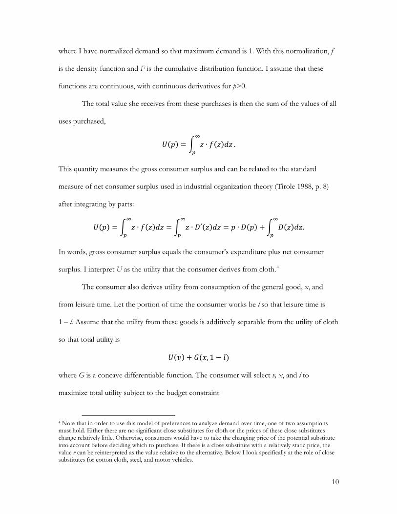
where I have normalized demand so that maximum demand is 1. With this normalization, f

is the density function and F is the cumulative distribution function. I assume that these

functions are continuous, with continuous derivatives for p>0.

The total value she receives from these purchases is then the sum of the values of all

uses purchased,

𝑈(𝑝) = � 𝑧 ∙ 𝑓(𝑧)𝑑𝑧∞

𝑝.

This quantity measures the gross consumer surplus and can be related to the standard

measure of net consumer surplus used in industrial organization theory (Tirole 1988, p. 8)

after integrating by parts:

𝑈(𝑝) = � 𝑧 ∙ 𝑓(𝑧)𝑑𝑧∞

𝑝= � 𝑧 ∙ 𝐷′(𝑧)𝑑𝑧

∞

𝑝= 𝑝 ∙ 𝐷(𝑝) + � 𝐷(𝑧)𝑑𝑧.

∞

𝑝

In words, gross consumer surplus equals the consumer’s expenditure plus net consumer

surplus. I interpret U as the utility that the consumer derives from cloth.4

The consumer also derives utility from consumption of the general good, x, and

from leisure time. Let the portion of time the consumer works be l so that leisure time is

1 – l. Assume that the utility from these goods is additively separable from the utility of cloth

so that total utility is

𝑈(𝑣) + 𝐺(𝑥, 1 − 𝑙)

where G is a concave differentiable function. The consumer will select v, x, and l to

maximize total utility subject to the budget constraint

4 Note that in order to use this model of preferences to analyze demand over time, one of two assumptions must hold. Either there are no significant close substitutes for cloth or the prices of these close substitutes change relatively little. Otherwise, consumers would have to take the changing price of the potential substitute into account before deciding which to purchase. If there is a close substitute with a relatively static price, the value v can be reinterpreted as the value relative to the alternative. Below I look specifically at the role of close substitutes for cotton cloth, steel, and motor vehicles.

11

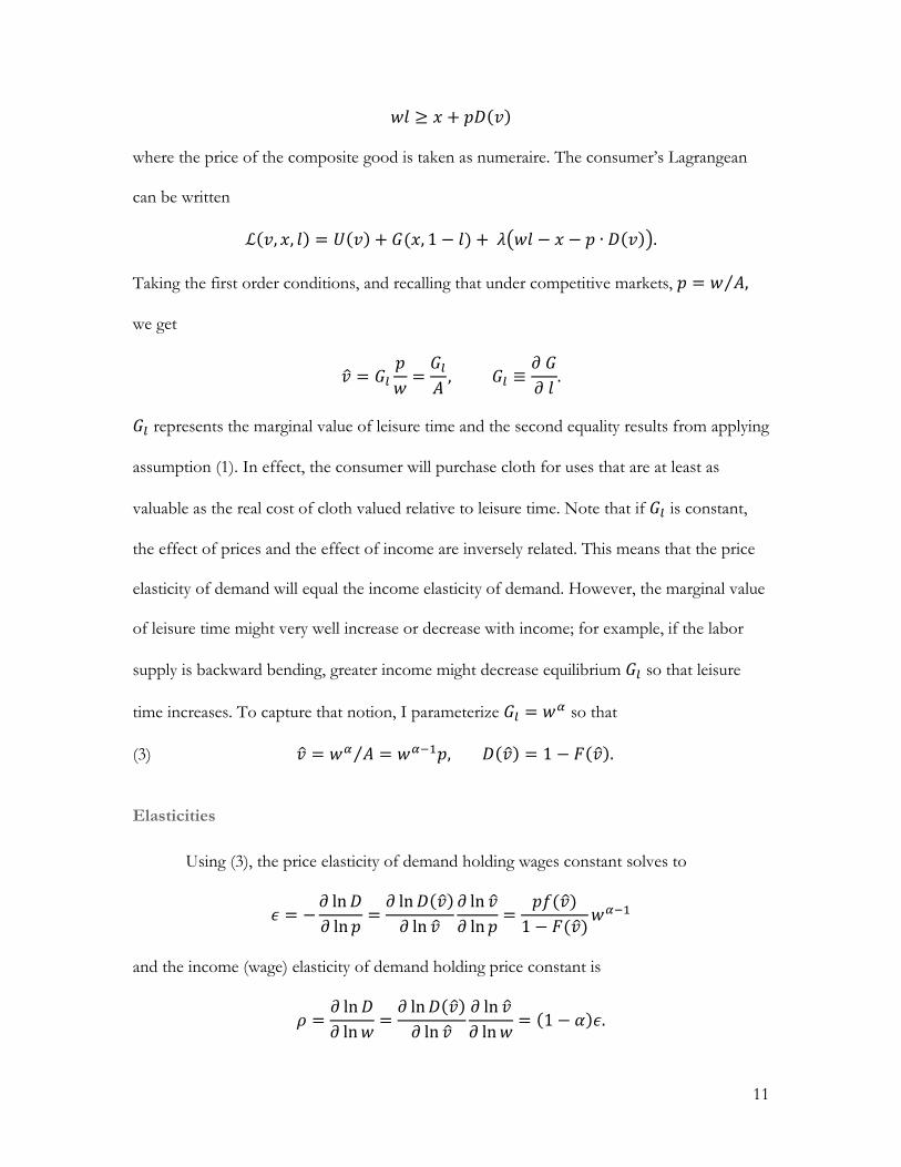
𝑤𝑙 ≥ 𝑥 + 𝑝𝐷(𝑣)

where the price of the composite good is taken as numeraire. The consumer’s Lagrangean

can be written

ℒ(𝑣, 𝑥, 𝑙) = 𝑈(𝑣) + 𝐺(𝑥, 1 − 𝑙) + 𝜆�𝑤𝑙 − 𝑥 − 𝑝 ∙ 𝐷(𝑣)�.

Taking the first order conditions, and recalling that under competitive markets, 𝑝 = 𝑤 𝐴⁄ ,

we get

𝑣� = 𝐺𝑙𝑝𝑤

=𝐺𝑙𝐴

, 𝐺𝑙 ≡𝜕 𝐺𝜕 𝑙

.

𝐺𝑙 represents the marginal value of leisure time and the second equality results from applying

assumption (1). In effect, the consumer will purchase cloth for uses that are at least as

valuable as the real cost of cloth valued relative to leisure time. Note that if 𝐺𝑙 is constant,

the effect of prices and the effect of income are inversely related. This means that the price

elasticity of demand will equal the income elasticity of demand. However, the marginal value

of leisure time might very well increase or decrease with income; for example, if the labor

supply is backward bending, greater income might decrease equilibrium 𝐺𝑙 so that leisure

time increases. To capture that notion, I parameterize 𝐺𝑙 = 𝑤𝛼 so that

(3) 𝑣� = 𝑤𝛼 𝐴⁄ = 𝑤𝛼−1𝑝, 𝐷(𝑣�) = 1 − 𝐹(𝑣�).

Elasticities

Using (3), the price elasticity of demand holding wages constant solves to

𝜖 = −𝜕 ln𝐷𝜕 ln𝑝

=𝜕 ln𝐷(𝑣�)𝜕 ln 𝑣�

𝜕 ln 𝑣�𝜕 ln𝑝

=𝑝𝑓(𝑣�)

1 − 𝐹(𝑣�)𝑤𝛼−1

and the income (wage) elasticity of demand holding price constant is

𝜌 =𝜕 ln𝐷𝜕 ln𝑤

=𝜕 ln𝐷(𝑣�)𝜕 ln 𝑣�

𝜕 ln 𝑣�𝜕 ln𝑤

= (1 − 𝛼)𝜖.

12

These elasticities change with prices and wages or alternatively with changes in labor

productivity, A. The changes can create an inverted-U in employment. Specifically, if the

price elasticity of demand, 𝜖, is greater than 1 at high prices and lower than 1 at low prices,

then employment will trace an inverted U as prices decline with productivity growth. At high

prices relative to income, productivity improvements will create sufficient demand to offset

job losses; at low prices relative to income, they will not.

A preference distribution function with this property can generate a kind of industry

life cycle as technology continually improves labor productivity over a long period of time.

An early stage industry will have high prices and large unmet demand, so that price decreases

result in sharp increases in demand; a mature industry will have satiated demand so further

price drops only produce an anemic increase in demand.

A necessary condition for this pattern is that the price elasticity of demand must

increase with price over some significant domain, so that it is smaller than 1 at low prices but

larger than 1 at high prices. It turns out that many distribution functions have this property.

This can be seen from the following propositions (proofs in the Appendix):

Proposition 1. Single-peaked density functions. If the distribution density function, f, has a single peak at 𝑝 = �̅�, then 𝜕𝜕

𝜕𝑝≥ 0 ∀ 𝑝 < �̅�.

Proposition 2. Common distributions. If the distribution is normal, lognormal, exponential or uniform, there exists a 𝑝∗such that for 0 < 𝑝 < 𝑝∗, 𝜖 < 1, and for 𝑝∗ < 𝑝, 𝜖 > 1.

These propositions suggest that the model of demand derived from distributions of

preferences might be broadly applicable. The second proposition is sufficient to create the

inverted U curve in employment as long as the price starts above 𝑝∗ and declines below it.

13

Empirical estimates

This very simple model does not consider numerous factors that might influence

demand. It does not consider the role of close substitutes or the effect of the business cycle

on demand. New technology might create new products that generate new demand, altering

the distribution, or new substitutes that decrease demand. Global trade might alter

downstream industries, affecting the demand for intermediate goods such as cloth or steel.

Nevertheless, the model appears to predict actual demand over a historical timeframe

reasonably well.

Assuming that the preference distribution is lognormal, I estimate the per capita

demand functions for these three commodities (see Bessen 2017 for details). The model fits

the data quite closely, realizing R-squareds of .982 or higher. Using these predictions, I

estimate the price elasticity of demand at each end of the estimation sample:

Cotton Steel Automotive Year Elasticity Year Elasticity Year Elasticity 1810 2.13 1860 3.49 1910 6.77 1995 0.02 1982 0.16 2007 0.15

The demand was initially highly elastic, but became highly inelastic.

Using estimated per capita demand, labor demand can be calculated incorporating

population size, import penetration, labor productivity and hours worked. These estimates

are shown as the solid lines in Figure 1. The estimates appear to be accurate over long

periods of time. There are notable drops in employment during the Great Depression and

excess employment in motor vehicles during World War II. Finally, employment falls below

the estimates when globalization takes a bite out of employment in textiles after 1995, and

steel after 1982.

14

Thus, even though this overly simple model does not account for all of the factors

that affect demand, it nevertheless provides a succinct explanation of the inverted U in

employment in these manufacturing industries.

Implication for AI

The importance of demand

Although the model presented here appears to provide a good explanation for how

demand mediated the impact of technology in the past, what is the relevance of this analysis

for new technologies? There is, of course, no guarantee that AI or other new technologies

will be applied in markets with preference distributions similar to those of the textile, steel

and automotive industries.

The relevance of this history is more general. Specifically, the responsiveness of

demand is key to understanding whether major new technologies will decrease or increase

employment in affected industries. Productivity-enhancing technology will increase industry

employment if product demand is sufficiently elastic. If the price elasticity of demand is

greater than one, the increase in demand will more than offset the labor saving effect of the

technology. And demand will likely be sufficiently elastic if the technology is addressing large

unmet needs affecting people with diverse preferences and uses for the technology. This

situation corresponds to the upper tail of the distribution function. If, on the other hand, AI

is targeted at more satiated markets, then jobs will be lost in the affected industries, although

not necessarily in the economy as a whole.

The pace of change of a new technology is not sufficient by itself to determine the

impact of that technology on employment. For example, a common view holds that faster

technical change is more likely to eliminate jobs. Some people argue that because of Moore’s

15

Law, the rate of change will be fast for AI and this will cause unemployment (Ford 2015).

However, my analysis highlights the importance of demand in mediating the impact of

automation. If demand is sufficiently elastic and AI does not completely replace humans,

then technical change will create jobs rather than destroy them. In this case, a faster rate of

technical change will actually create faster employment growth rather than job losses.

The demand response to AI is, of course, an empirical question and, therefore, an

important part of the AI research agenda.

Research agenda

To understand the interaction between AI and demand over the next 10 or 20 years,

empirical researchers will need answers to several specific questions.

First, to what extent will AI replace humans and to what extent will it, instead,

merely augment human capabilities? That is, to what extent will AI completely automate

occupations and to what extent will it, instead, merely automate some, but not all, tasks

performed by an occupation. If humans are completely replaced, demand no longer affects

employment because there isn’t any demand for humans. In the past, despite extensive

productivity growth, technology has almost always only partially automated work. Consider

what happened to the 271 detailed occupations used in the 1950 census by 2010. Most

occupations listed then still exist in some form (sometimes grouped differently) today. Some

occupations were eliminated for a variety of reasons. In many cases, demand for the

occupational services declined (e.g., boardinghouse keepers); in some cases, demand declined

because of technological obsolescence (e.g., telegraph operators). This, however, is not the

same as automation. In only one case — elevator operators — can the decline and

16

disappearance of an occupation be largely attributed to automation. Nevertheless, this 60-

year period witnessed extensive automation; it was just mostly partial automation.

This same pattern is likely to be true for AI over the next 10 or 20 years for the

simple reason that although AI can outperform humans on some tasks, today’s AI fails

miserably at other tasks that humans perform. A casual review of current developments

suggests that over the near term AI may be able to completely automate some jobs of drivers

and warehouse workers, but most AI applications are targeted toward automating just some

subset of tasks performed by specific occupations. Nevertheless, a more rigorous empirical

investigation is needed to measure the extent to which AI is bringing or will bring complete

versus partial automation.

To the extent that automation continues to be partial rather than complete in the

near term, demand will be key. This raises a second question: to what extent will the effect of

AI on demand and employment during the next 10 or 20 years be similar to the effect that

AI and computer automation generally had over the last several decades? Computers have

been used to automate work in activities such as accounting and loan making since the

1950s. The first fully automatic loan application system was installed in 1972. In 1987, an

artificial intelligence system was first put into commercial operation in a system used to

detect credit fraud. Since then, AI applications have been used to automate a variety of tasks

in other industries and occupations, such as the electronic discovery of legal documents for

litigation.

This means that we already have some evidence of the effects of AI and computer

automation generally. It does not seem that computer automation or AI has so far led to

significant job losses; the booming market for electronic discovery applications, for instance,

has been associated with an increase in the employment of paralegals. A few studies have

17

made estimates of the employment impact of computer technology (Gaggl and Wright 2017;

Akerman et al. 2015), finding, if anything, a modest increase in employment following

technology adoption.5 Further studies could deepen our understanding of the impact of

computer automation on employment, and how this impact differs across occupations and

industries.

Also, we need to understand how AI applications in the near future will differ from

those of the recent past. The model above provides a framework to analyze this question. In

particular, to the extent that the new applications target the same services and industries as

did the computer automation of the recent past, then we should expect the elasticity of

demand to remain similar over the next 10 or 20 years, perhaps with a modest decline. That

is, the elasticity of demand is not likely to change very quickly. On the other hand, AI might

introduce entirely new products and services that tap into otherwise unmet needs and wants.

In this case, there may be new and unanticipated sources of employment growth. Research

can help determine the extent of change in the sorts of applications, occupations and

industries affected by new AI applications that are also addressed by existing technologies.

To the extent that AI creates wholly new applications, prediction will be more difficult.

Indeed, in the past, predictions about technological unemployment have reliably failed to

anticipate major new applications of technology and major new sources of demand.

A critical aspect of this research concerns the unevenness of the potential impact of

AI. While AI might not create overall unemployment in the near future, it will likely

eliminate jobs in some occupations while creating new jobs in others. The need to retrain

and transition workers to new occupations, sometimes in new locations, might be highly

disruptive even though the total employment rate remains high.

5 And, importantly, impacts that differed across skill groups.

18

Finally, it is important to note that this analytical framework and research agenda are

very much limited to the next 10 or 20 years for two reasons. First, beyond a couple of

decades, markets might well become saturated. Suppose, for example, that demand is highly

elastic for many financial, health and other services today so that information technology

increases employment in these markets. If AI rapidly reduces costs or improves the quality

of these services, the elasticity of demand will decline. That is, these markets might see the

kind of reversals in employment growth seen in Figure 1.

Second, in the future, AI might very well be able to completely replace many more

occupations. Then the effect of AI on demand will no longer matter for these occupations.

For now, however, understanding how and where AI affects demand is critical to

understanding employment effects.

19

Appendix

Propositions

To simplify notation, let the wage remain constant at 1. Then

𝜖(𝑝) =𝑝 𝑓(𝑝)

1 − 𝐹(𝑝)

so that

𝜕 𝜖(𝑝)𝜕 𝑝

=𝑓′𝑝

1 − 𝐹+

𝑓2𝑝(1 − 𝐹)2 +

𝑓1 − 𝐹

= 𝜖 �𝑓′𝑓

+𝑓

1 − 𝐹+

1𝑝�

Note that the second and third terms in parentheses are positive for 𝑝 > 0; the first term

could be positive or negative. A sufficient condition for 𝜕𝜕𝜕𝑝≥ 0 is

(A1)

𝑓′𝑓

+𝑓

1 − 𝐹≥ 0.

Proposition 1. For a single peaked distribution with mode �̅�, for 𝑝 < �̅� , 𝑓′ ≥ 0 so that

𝜕𝜕𝜕𝑝≥ 0 .

Proposition 2. For each distribution, I will show that

𝜕𝜖𝜕𝑝

≥ 0, lim𝑝→0

𝜖 = 0, lim𝑝→∞

𝜖 = ∞.

Taken together, these conditions imply that for sufficiently high price, 𝜖 > 1, and for a

sufficiently low price, 𝜖 < 1.

a. Normal distribution

𝑓(𝑝) =1𝜎𝜑(𝑥), 𝐹(𝑝) = Φ(𝑥), 𝜖(𝑝) =

𝑝𝜎

𝜑(𝑥)(1 −Φ(𝑥))

, 𝑥 ≡𝑝 − 𝜇𝜎

20

where 𝜑 and Φ are the standard normal density and cumulative distribution functions

respectively. Taking the derivative of the density function,

𝑓′

𝑓+

𝑓1 − 𝐹

= −𝑥𝜎

+𝜑(𝑥)

𝜎 �1 −Φ(𝑥)�.

A well-known inequality for the normal Mills’ ratio (Gordon 1941) holds that for x>0,6

(A2)

𝑥 ≤𝜑(𝑥)

1 −Φ(𝑥).

Applying this inequality, it is straightforward to show that (A1) holds for the normal

distribution. This also implies that lim𝑝→∞ 𝜖 = ∞. By inspection, 𝜖(0) = 0.

b. Exponential distribution

𝑓(𝑝) ≡ 𝜆𝑒−𝜆𝑝, 𝐹(𝑝) ≡ 1 − 𝑒−𝜆𝑝, 𝜖(𝑝) = 𝜆𝑝, 𝜆,𝑝 > 0.

Then

𝑓′

𝑓+

𝑓1 − 𝐹

= −𝜆 + 𝜆 = 0

so (A1) holds. By inspection, 𝜖(0) = 0 and lim𝑝→∞ 𝜖 = ∞.

c. Uniform distribution

𝑓(𝑝) ≡1𝑏

, 𝐹(𝑝) ≡𝑝𝑏

, 𝜖(𝑝) =𝑝

𝑏 − 𝑝, 0 < 𝑝 < 𝑏

so that

𝑓′

𝑓+

𝑓1 − 𝐹

=1

𝑏 − 𝑝> 0.

By inspection, 𝜖(0) = 0 and lim𝑝→𝑏 𝜖 = ∞.

6 I present the inverse of Gordon’s inequality.

21

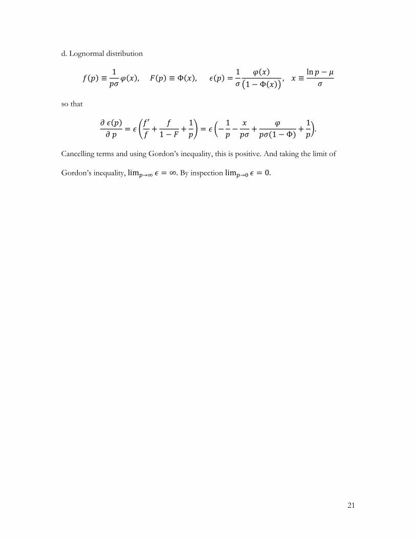
d. Lognormal distribution

𝑓(𝑝) ≡1𝑝𝜎

𝜑(𝑥), 𝐹(𝑝) ≡ Φ(𝑥), 𝜖(𝑝) =1𝜎

𝜑(𝑥)�1 −Φ(𝑥)�

, 𝑥 ≡ln𝑝 − 𝜇

𝜎

so that

𝜕 𝜖(𝑝)𝜕 𝑝

= 𝜖 �𝑓′𝑓

+𝑓

1 − 𝐹+

1𝑝� = 𝜖 �−

1𝑝−

𝑥𝑝𝜎

+𝜑

𝑝𝜎(1 −Φ)+

1𝑝�.

Cancelling terms and using Gordon’s inequality, this is positive. And taking the limit of

Gordon’s inequality, lim𝑝→∞ 𝜖 = ∞. By inspection lim𝑝→0 𝜖 = 0.

22

References

Acemoglu, Daron, and Veronica Guerrieri. "Capital deepening and nonbalanced economic growth." Journal of political Economy 116.3 (2008): 467-498.

Akerman, Anders, Ingvil Gaarder, and Magne Mogstad. "The skill complementarity of broadband internet." The Quarterly Journal of Economics 130, no. 4 (2015): 1781-1824.

Baumol, William J. "Macroeconomics of unbalanced growth: the anatomy of urban crisis." The American economic review (1967): 415-426.

Bessen, James E. "How computer automation affects occupations: Technology, jobs, and skills." (2016).

Bessen, James. “Automation and Jobs: When Technology Boosts Employment,” Boston Univ. School of Law, Law and Economics Research Paper No. 17-09.

Boppart, Timo. "Structural Change And The Kaldor Facts In A Growth Model With Relative Price Effects And Non-Gorman Preferences." Econometrica (2014): 2167-2196.

Buera, Francisco J., and Joseph P. Kaboski. "Can traditional theories of structural change fit the data?." Journal of the European Economic Association 7.2‐3 (2009): 469-477.

Clark, Colin, The Conditions of Economic Progress. (1840) London: Macmillan.

Comin, Diego A., Danial Lashkari, and Martí Mestieri. Structural change with long-run income and price effects. No. w21595. National Bureau of Economic Research, 2015.

Dennis, Benjamin N., and Talan B. İşcan. "Engel versus Baumol: Accounting for structural change using two centuries of US data." Explorations in Economic history 46.2 (2009): 186-202.

Dupuit, Jules. “De la mesure de l’utilité des travaux publics” 1844, Annales des ponts et chaussées, v.8 (2 sem), p.332-75

Engel, Ernst (1857). "Die Productions- und Consumtionsverhältnisse des Königreichs Sachsen". Zeitschrift des statistischen Bureaus des Königlich Sächsischen Ministerium des Inneren. 8–9: 28–29.

Foellmi, Reto, and Josef Zweimüller. "Structural change, Engel's consumption cycles and Kaldor's facts of economic growth." Journal of monetary Economics 55.7 (2008): 1317-1328.

Ford, Martin. Rise of the Robots: Technology and the Threat of a Jobless Future. Basic Books (2015).

23

Gaggl, Paul, and Greg C. Wright. "A Short-Run View of What Computers Do: Evidence from a UK Tax Incentive." American Economic Journal: Applied Economics, (2017) 9(3): 262–294.

Gordon, Robert D. "Values of Mills' ratio of area to bounding ordinate and of the normal probability integral for large values of the argument." The Annals of Mathematical Statistics 12.3 (1941): 364-366.

Kollmeyer, Christopher. "Explaining Deindustrialization: How Affluence, Productivity Growth, and Globalization Diminish Manufacturing Employment 1." American Journal of Sociology 114.6 (2009): 1644-1674.

Kongsamut, Piyabha, Sergio Rebelo, and Danyang Xie. "Beyond balanced growth." The Review of Economic Studies 68.4 (2001): 869-882.

Lawrence, Robert Z., and Lawrence Edwards. "US employment deindustrialization: insights from history and the international experience." Policy Brief 13-27 (2013).

Lebergott, Stanley. "Labor Force and Employment 1800-1960." In Dorothy Brady, ed., Output, Employment and Productivity in the United States After 1800. National Bureau of Econonic Research, Studies in Income and Wealth 30 (1966).

Lewis, W. Arthur. "Economic development with unlimited supplies of labour." The manchester school 22.2 (1954): 139-191.

Matsuyama, Kiminori. "Agricultural productivity, comparative advantage, and economic growth." Journal of economic theory 58.2 (1992): 317-334.

Matsuyama, Kiminori. "Structural change in an interdependent world: A global view of manufacturing decline." Journal of the European Economic Association 7.2‐3 (2009): 478-486.

Matsuyama, Kiminori. "The rise of mass consumption societies." Journal of political Economy 110.5 (2002): 1035-1070.

Ngai, L. Rachel, and Christopher A. Pissarides. "Structural change in a multisector model of growth." The American Economic Review 97.1 (2007): 429-443.

Nickell, Stephen, Stephen Redding, and Joanna Swaffield. "The uneven pace of deindustrialisation in the OECD." The World Economy 31.9 (2008): 1154-1184.

Parker, William N., and Judith LV Klein. "Productivity growth in grain production in the United States, 1840–60 and 1900–10." Output, employment, and productivity in the United States after 1800. NBER, 1966. 523-582.

Rodrik, Dani. "Premature deindustrialization." Journal of Economic Growth 21.1 (2016): 1-33.

24

Rowthorn, Robert, and Ramana Ramaswamy. "Growth, trade, and deindustrialization." IMF Staff papers 46.1 (1999): 18-41.

Tirole, Jean. The theory of industrial organization. MIT press, 1988.

United States. Bureau of the Census. Historical Statistics Of The United States, Colonial Times To 1970. No. 93. US Department of Commerce, Bureau of the Census, 1975.

25

Figures

Figure 1. Production Employment in Three Industries

26

Figure 2. Manufacturing Share of the Labor Force

Sources: U.S. Bureau of the Census 1975; BLS Current Employment Situation. Labor force includes agricultural laborers