aging, labor supply and consumption - sectoral e … labor supply and consumption - sectoral e ects...
TRANSCRIPT

Aging, Labor Supply and Consumption -Sectoral Effects of Demographic Change in
Germany
Ute B. Volz∗
August 2008
The German population is forecast to become smaller and older over thenext few decades. Population aging as a consequence of demographic changewill influence the economy. This paper tries to quantify the effects in a com-putable general equilibrium model with 17 production sectors and heteroge-neous households based on German data from 2000. It analyzes the sectoraleffects of population aging stemming from two effects, namely a negative la-bor supply shock and a change in the composition of consumption demand.To the best of our knowledge it is the first paper to combine input-outputdata and matching micro level, i.e. household level data for Germany. Thesector affected most in this analysis is that of ‘health, education and socialservices’.
JEL Classification: C68, J11, O52, R15
Keywords: demographic aging, computable general equilibrium, sectoraldecomposition
∗Ruhr Graduate School in Economics (RGS Econ) & University of Duisburg-Essen - The author is grate-ful to her thesis supervisor Volker Clausen and also to Sebastian Rausch and Hannah Schurenberg forhelpful comments and encouragement. Financial support from the RGS is gratefully acknowledged.Contact information: phone: +49-201-1834507, email: [email protected]
1

1 Introduction
1 Introduction
As many other OECD countries Germany experiences a shift in its population com-position. Life expectancy rises, birth rates rather decline. Especially with the so calledBaby Boomers retiring and following generations considerably smaller in size populationaging is becoming a topic debated lively. According to United Nations (2002) the elderlydependency ratio in Germany will rise from 24.1 in 2000 to 54.7 in 2050, thus more thandouble. Quantifying the possible effects of these changes is the aim of this paper. In theliterature, demographic change used to be associated with population growth, a topicmainly linked to developing countries. Thus, several studies deal with topics related toeconomic development which is not the focus of this study.1 It is more the wide-rangingimpact on the Euro area economy2 and especially the central economic and social chal-lenges for Germany and industrialized countries in general as referred to in the EuropeanCentral Bank’s monthly bulletin for October 2006 and in Deutsche Bundesbank (2004).Aside from effects on pension schemes, especially pay-as-you-go systems, which are welldealt with in the literature already, there arise important structural changes on productmarkets, labor markets and financial markets from population aging.
Leaving aside financial markets this study focuses on product and labor markets. Heretwo aspects are of importance. First, population aging produces a negative labor supplyshock via workforce aging. Second, population aging comes with a perceptible structuralchange of household composition and with it final demand. The relative scarcity ofworkers will exert pressure on labor markets. The changed composition of householdtypes will have an impact on final demand. The economy’s (final) demand changes witha modified population composition as the proportion of the elderly will grow relative tothe younger and still labor active. Deutsches Institut fur Wirtschaftsforschung (2007)and Schaffnit-Chatterjee (2007), two rather recent studies for example, look closer at theconsumption spending behavior of the elderly. Thus the first effect leads to a supply-sidethe second to a demand-side shock to the system. With these effects a CGE analysisbecomes interesting.
The aim of this analysis is to explore the sectoral effects of population aging onGermany by taking into account both the supply-side and demand-side channels. Tothe best of our knowledge this is the first paper combining input-output data withhousehold level data for Germany to study the issue of demographic change. The modeldistinguishes between 17 production sectors and two household types. labor supply isendogenous as agents are endowed with time and can freely choose whether to use itfor leisure or for labor which means goods consumption. Similar studies can only befound in different areas, e.g. Boeters, Schnabel, and Gurtzgen (2006), an evaluation of asocial welfare reform in Germany or Boeters, Bohringer, Buttner, and Kraus (2006), anevaluation of value-added tax reform in Germany. Other related studies are Denton andSpencer (1999); Borsch-Supan (2003); Batini, Callen, and McKibbin (2006); Krueger and
1The interested reader may refer to for example Bloom, Canning, and Malaney (1999); Bloom andCanning (2006); Kelley and Schmidt (2001); Bloom and Canning (2004); Bloom, Canning, Fink, andFinlay (2006).
2See European Central Bank (2006).
2

2 Model Description
Ludwig (2007); Fougere, Mercener, and Merette (2007). In these models consumptiondemand changes are induced by a varying age structure of consumers. However, exceptfor Fougere, Mercener, and Merette (2007) they only take into account very few sectors.In Krueger and Ludwig (2007) for example there is only one consumption good and amarket each, one for labor services and one for capital services. A rather unsatisfactoryapproach if focus lies on sectoral effects of population aging.
Very similar to our study is that by Fougere, Mercener, and Merette (2007). Theyset up a model with fourteen industrial sectors of production activities, three differenttypes of labor, ten occupational groups and five levels of qualification. As these au-thors state: “Little previous work has considered examining the combination of supplyand final-demand channel effects from population aging and using a general equilibriumframework. To the best of our knowledge, none have explored the sectoral and labormarket implications of population aging at the occupational skill levels.” (Fougere, Mer-cener, and Merette, 2007, p. 691) Their OLG model is calibrated to Canadian data. Ourstudy is a detailed sectoral analysis with German data and allows for endogenous laborsupply. Methodologically it is built straightforward as a static model. This will in laterstudies allow for a comparison of outcomes with different methodologies. Insights fromthis study are not confined to Germany as the effect of population aging will be similarin most industrialized countries. Most industrialized countries will be affected similarly.
The paper is structured as follows. Section 2 gives a detailed description of the model.Section 3 depicts the data used including the necessary adjustments conducted. Section4 reports and discusses the simulation results, followed by a concluding section withpolicy suggestions and some directions for future research.
2 Model Description
An economy-wide general equilibrium model contains all factor and commodity marketsas well as all economic agents. Thus, as demand and supply depend on the relativeprices of all other factor and goods markets, a CGE model is capable of taking intoaccount all essential interactions. CGE models are often used in development economics,as they are usually calibrated to a (one point in time) social accounting matrix andthus can help overcome data problems which persist in developing countries. Germanyis a country with a sound data basis. However, even for Germany it is hard to findconsistent production and household consumption data. Thus, a CGE model, calibratedto a one point in time SAM in contrast to an econometric analysis is appropriate evenfor Germany as data requirements are more appropriate for the current data situation.
In this model consumers are utility maximizers and producers profit maximizers. Mar-kets are assumed to be perfectly competitive and capital and labor are mobile acrosssectors. On the production side the economy is constructed of 17 production sectors.Production takes place using nested constant elasticity of substitution (CES) produc-tion and transformation (CET) functions with primary factors and intermediates. TheArmington assumption is used for modeling international trade in a way that foreign andhome production form final domestic consumption goods via a CES production function.
3

3 Data
In a similar fashion home production produces final domestic and export products witha CET production function. Germany is modeled as a small country and is thus a pricetaker on world markets.
There are two types of consumers, working and non-working, i.e. active and retiredhouseholds. They are endowed with capital and time. The latter they can transforminto leisure or labor (which means goods consumption). Capital and labor are primaryfactors. There is a government which collects product taxes and a lump sum transferfrom the model household type ‘working’/‘active’. This household type is the main actorin this model. It is endowed with most of the primary factors and makes all lump sumpayments in order to close the model, i.e. concerning the balance of payments (surplus),the government deficit and investments. In the base model, the household type ‘non-working’/‘retired’ also receives a lump sum transfer to the amount of their consumptionspending (according to household spending data). Both household types are endowedwith time which they can both transform into labor supply. However, the amount oftime transferred into labor supply is different within these two groups, representingdifferent preferences for leisure and the fact that the retired household type representspensioners and retirees who normally do not work.
Time endowment is proportional to the weight of the household type in the model andit is the parameter which is used to simulate demographic change. In accordance withpopulation projections the number of households within the two groups changes andwith it the time endowment of each household type in the model. The analysis is basedon comparative runs which simulate population aging by decreasing ‘active’ householdsand increasing ‘retired’ households in the model according to table 3.
Algebraically the model is set up in the mixed complementarity format. A CGE modelas described above could be set up as a system of simultaneous linear or non-linearequations. 3 For increased readability of this paper the model equations are shown laterin appendix A.
3 Data
The model is calibrated to German input output data for the year 2000. These aretaken from Klose, Opitz, and Schwarz (2005). The numbers are based on the concept ofnational accounting not on consumer surveying like the EVS4. Intuitively these data fitbetter for analysis dealing with household consumption, but as Lehmann (2004) statesthere are several problems with these data which are especially prevalent if the analysisis rather concerned with statements concerning the national economy as a whole. 5
3The equivalence of the formulation as a mixed complementarity problem has been shown by Mathiesen(1985). This format has the advantage of dealing easily with corner solutions. See Mathiesen (1985);Rutherford (1995) for more about the mixed complementarity format in CGE models.
4Erwerbs- und Verbrauchsstichprobe, data panel on private household spending collected by the Statis-tisches Bundesamt.
5Problems with the EVS in contrast to national accounting data as stated in Lehmann (2004) arefor example: dealing in second-hand goods produces double counting of these goods/transactions,certain positions can only be added and adjusted on the level of national accounting, examples
4

3 Data
As household consumption data are only available disaggregated to at most 17 sectors,the 71 available production sectors are aggregated to match those 17 sectors as can beseen in table 1.
Consumption sector Statistical Classification of Products by Activityaggregates in the European Economic Community
agricultural productsagricultural products; forestry products; fish,sea foods and trapping products
miningcoal and peat products; petroleum products,ores; mining products
food, beverages, tobacco food; beverages; tobacco
textiles, clothing, leather textiles; clothing; leather
wood, paper, printinglumber and wood products; wood pulp, paperand paper products; printing and publishing
petroleum and chemical petroleum and coal products; chemical,products pharmaceuticals and chemical products
metals primary and other metal products
machinery, vehicles, appliancesmachinery and equipment; motor vehicles, othertransportation equipment and parts; electrical,electronic and communication products
furniture, jewelry, furniture and fixtures; toys; musical instruments;musical instruments secondary commodities
energy, water, construction electricity, long-distance heating; gas; water; construction
trade services (s.) trade services
accommodation and leisure s. hotel and restaurant industry services
traffic and news services transportation and information services
finance and insurance s. finance and insurance services
real estate and business s. real estate and business services
health, education and social s. health services; education services; sanitation services
public administration, defence public administration services; social services;and cultural s. cultural, sports and entertainment services; other services
Table 1: Mapping into the 17 aggregated sectors
3.1 Data Adjustments
The data compiled by Klose, Opitz, and Schwarz (2005) are adjusted to satisfy therequirements of a social accounting matrix which is a major advantage for CGE modelingas the adjustment procedure undertaken by statistical experts ensures that consumptionand production data match. Nonetheless, there remain some further adjustments to bemade, subject to the distinct features of this model. One is the lack of an intertemporalconsumption/savings decision. In this model there is a sector ’savings’ which producesthe good ’savings’. This is consumed by the households (in the base model only by active
are service fees for insurances and betting and lotteries, household surveys suffer from systematicshortcomings as ‘problem household’ (long term care patients, socially disadvantaged, high earners)are underrepresented, self-recording in form of a book of household accounts leads to a change inbehavior, underreporting of low value and non-home consumption.
5

3 Data
households) but savings decisions have no intertemporal background. Another concernschanges in inventory stock. These are of a dynamic nature and cannot exist in a staticmodel. For ease of calculation and since the bare numbers are comparably negligiblethey are added to the households’ final consumption. The same applies to expendituresof private non-profit organizations which comprise almost only services.
A comparison of data for the usage of primary factors in the German input-outputtable with data for capital intensity from Institut der deutschen Wirtschaft Koln (2007)yields considerable differences. Due to a lack of more accurate data the study remainsbased on the most consistent available data taken from Klose, Opitz, and Schwarz (2005).
Consumption spending patterns
‘active’ ‘old’agricultural products 1.4% 1.8%mining 0.4% 0.5%food, beverages, tobacco 8.4% 9.7%textiles, clothing, leather 3.6% 2.7%wood, paper, printing 2.1% 2.3%petroleum and chemical products 3.7% 2.8%metals 0.4% 0.5%machinery, vehicles, appliances 7.8% 5.6%furniture, jewelry, musical instruments 2.1% 2.1%energy, water, construction 2.3% 3.4%trade services 18.3% 15.2%accommodation and leisure services 5.0% 5.8%traffic and news services 5.3% 6.0%finance and insurance services 6.4% 4.6%real estate and business services 20.7% 17.7%health, education and social services 5.5% 12.5%public administration, defence and cultural services 6.4% 7.0%
Table 2: Consumption spending by household type and sector
On the consumption side the data comprise self-employed households (7%), workinghouseholds (47%), retired and pensioner households (36%), and households of unem-ployed or otherwise dependent on social security payments (10%). Except for retiree andpensioner households the distribution of 1-, 2-, 3-, 4-, or 5 and more people householdsis very similar. Only in the afore mentioned group the 1- and 2-people households dom-inate. This poses an inconvenience in comparing population projections on per capitabasis and on household basis but is taken into account in the aging mechanism used inthis study. For the base version of the model the self-employed households and the work-ing households have been combined and classified as ‘working’/‘active’ while the retiredand pensioner households are classified as ‘non-working’/‘retired’. The rest is proratedaccording to group size.
With this segmentation of consumption spending by household type and economicsector in this model results in what is shown in table 2. Numbers are percentage ofdisposable income used for consumption goods.
Population projections are usually made on per capita bases. These projections needto be modified in order to be useful for this study, as here whole households are usedon the consumption side. Accounting for differences in household size and conventionalpopulation projections for Germany the development as stated in table 3 and figure 1is calculated from Klose, Opitz, and Schwarz (2005); United Nations, Department of
6

3 Data
active retired totalscenario 1-W1 16,202.84 19,045.19 35,248.02scenario 1-W2 17,859.63 19,840.04 37,699.67scenario 2-W1 16,234.22 20,212.01 36,446.22scenario 2-W2 17,894.26 21,026.38 38,920.64scenario 3-W1 17,363.76 19,117.76 36,481.52scenario 3-W2 19,086.78 19,915.64 39,002.42scenario 4-W1 17,398.59 20,284.79 37,683.38scenario 4-W2 19,120.64 21,101.82 40,222.47scenario 5-W1 15,595.14 19,008.94 34,604.08scenario 5-W2 17,211.12 19,802.03 37,013.15scenario 6-W1 15,628.45 20,176.02 35,804.47scenario 6-W2 17,246.36 20,988.47 38,234.84year 2000 20,155 17,530 37,685
Table 3: number of households in population forecasts
Economic and Social Affairs, Population Division (2006); Bundesamt fur Bauwesen undRaumordnung (2005) and used in this study. The base are projections by Bundesamtfur Bauwesen und Raumordnung (2005) which are then distributed onto the modelhousehold types according to Klose, Opitz, and Schwarz (2005) and United Nations,Department of Economic and Social Affairs, Population Division (2006).6 The twelvedifferent scenarios mean:
scenario 1: constant birth rate, basic life expectancy assumption
scenario 2: constant birth rate, high life expectancy
scenario 3: slightly rising birth rate, basic life expectancy assumption
scenario 4: slightly rising birth rate, high life expectancy
scenario 5: slightly falling birth rate, basic life expectancy assumption
scenario 6: slightly falling birth rate, high life expectancy
variation W1: low immigration
variation W2: high immigration
As production data are stated at manufacturing cost, consumption data, however, atpurchase prices there remained some further adjustment. The consumption data corre-spond to 11% taxes, 16% trade services and 73% consumption at manufacturing cost.Hence, they have been divided into trade services and and true consumption spendingplus a tax on all goods.
6A detailed description can be found in appendix C.
7

4 Results
-
10,000
20,000
30,000
40,000
50,000
scen
ario
1-W
1
scen
ario
1-W
2
scen
ario
2-W
1
scen
ario
2-W
2
scen
ario
3-W
1
scen
ario
3-W
2
scen
ario
4-W
1
scen
ario
4-W
2
scen
ario
5-W
1
scen
ario
5-W
2
scen
ario
6-W
1
scen
ario
6-W
2
household head under 65 household head over 65
Figure 1: population forecast scenarios
4 Results
When simulating the demographic change of Germany in the model, the population ex-periences two different changes at the same time. One is a general fall of population sizethe other a change in the relative importance of household types. If not combined withany other effect this means a smaller labor supply but also a smaller number of con-sumers. Thus, in relative terms, everything (e.g. relative prices and relative quantities)could be the same. The other effect of demographic change is a shift from ‘active’ towards‘retired’ households. Demographic change in Germany means that there are less ‘active’people in absolute and relative terms. This holds for all twelve scenarios and can be seenin table 3. This reduction in the workforce is only one effect of demographic change. Asthe population composition changes gradually towards a greater share of elderly also theaggregate demand composition changes towards the preferences of ‘retired’ households.They form a greater part of the total population, thus aggregate demand will probablyreflect their preferences more than before.
The following section shows results of the model. A sensitivity analysis was undertakenand is described in appendix D. Section 4.2 takes apart the two effects of the model,namely the age effect and the population size effect.
8

4 Results
850
900
950
1,000
1,050
1,100
1,150
1w1
1w2
2w1
2w2
3w1
3w2
4w1
4w2
5w1
5w2
6w1
6w2
2050 2000
Figure 2: overall employment
4.1 Overall Model Results
As in the model labor is endogenous households can decide themselves how much of theirtime they use for labor and how much for leisure. Retired households are less willing touse their time for labor than active households. This way retired households stay retiredand cannot go back and join the workforce again. Although active households thus bearthe burden of adjustment they are modeled to be more flexible than retired householdsbut not fully flexible - resembling the fact that there are limits to the maximum amountof hours an ordinary worker may choose to work per week. This fact is not assumed tovanish (completely) until 2050.
Therefore, it is not surprising, that figure 2 resembles in the total amount of laboremployed in the economy the idfferent population sizes according to the various scenar-ios7. Nonetheless, as figures 3 and 4 show, it is mostly hte active households that bearthe burden of adjustment in that they choose to work relatively more in all scenarioswhile the retired stay about at their benchmark level - and even choose to work less inscenario 4-W2. The ratio of labor supplied to total time endowment of the householdtype ‘active’ increases for example from 50.4% to 55.3% in scenario 2-W1. The sameratio for household type ‘retired’ increases only from slightly more than 4.9% to 5% inthe same scenario, which is not even an increase of relative size of 2%.
7For ease of result interpretation it has been abstracted from increasing labor productivity but thisfeature can easily be incorporated into the model.
9

4 Results
45%
50%
55%
60%
1w1
1w2
2w1
2w2
3w1
3w2
4w1
4w2
5w1
5w2
6w1
6w2
2050 2000
Figure 3: time w
4.8%
4.9%
5.0%
5.1%
1w1
1w2
2w1
2w2
3w1
3w2
4w1
4w2
5w1
5w2
6w1
6w2
2050 2000
Figure 4: time n
10

4 Results
Moving from these general model results to the more disaggregated sphere of thedifferent sectors the development of relative prices is shown in table 4 for scenario 2-W1which we believe to be the most probable8.
Price change over the model horizonagricultural products -5.8 %mining -4.1 %food, beverages, tobacco -5.1 %textiles, clothing, leather -4.0 %wood, paper, printing -5.0 %petroleum and chemical products -4.5 %metals -3.9 %machinery, vehicles, appliances -3.6 %furniture, jewelry, musical instruments -4.0 %energy, water, construction -4.6 %trade services -4.5 %accommodation and leisure services -4.6 %traffic and news services -5.0 %finance and insurance services -4.6 %real estate and business services -7.8 %health, education and social services -3.7 %public administration, defence and cultural services -3.9 %
Table 4: Price changes over the model horizon
As it is necessary in a CGE model to choose one good or factor price as a numeraireonly relative prices can be shown. In this case the price of labor was chosen as a nu-meraire. As labor gets scarce relative to capital, the other factor and is thus becomingrelatively more expensive it is not surprising that all goods prices fall relative to bench-mark prices of 2000 as the numeraire in 2050 is the relatively most expensive factor inthe model economy. Any other commodity could have been chosen as numeraire. Thiswould certainly influence some prices to be positive and others to still be negative. Thiswas not done here because thehuman brain would attach a different meaning to positiveand negative changes although the exact distinction of which price would be shown torise and which to fall would heavily depend on the numeraire chosen which would iselfbe just a arbitrary as choosing the price of labor.
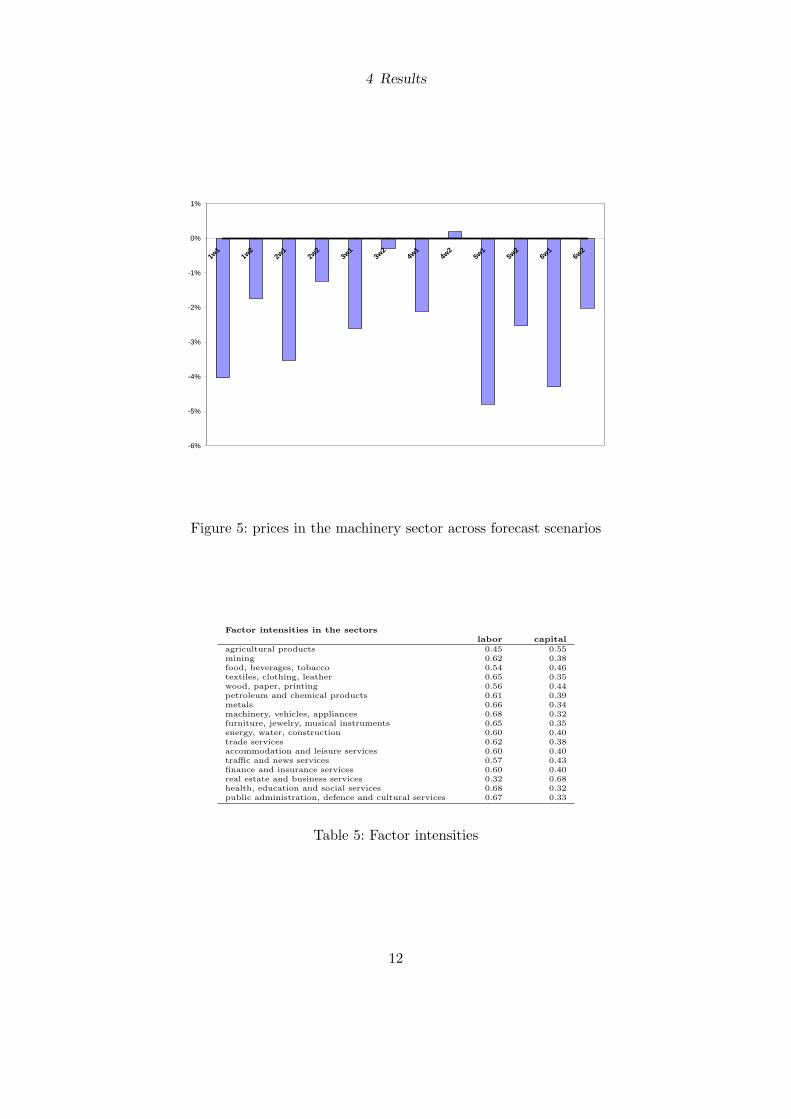
What is interesting is that the health and social services sector is relatively seen themost expensive. This can be explaied by the shift in demand as well as the smaller supplyof labor and this sectors high factor intensity in the factor labor. Factor intensities canbe seen in table 5
The agricultural sector and the real estate services sector are capital intense while theother sectors are to varying degrees labor intensive in their production9.
Sectoral labor usage for the health and the agricultural sectors - two rather differentsectors according to factor intensities - is shown in figure 6. An overview for all sectorsin scenario 2-W1 is depicted in tables 6-9.
Clearly the effect on the health sector is one of the smallest across all four tables.‘Public administration’ and ‘energy’ are two other sectors affected in a similar fashion,while the ‘textiles, clothing, leather’sector is one of the most affected sectors, somethingthat is in accordance with the historical development.
8The variation of these results across the different forecast scenarios is visible in figure 5.9The calculation of the factor intensities can be found in appendix B
11
4 Results
-6%
-5%
-4%
-3%
-2%
-1%
0%
1%
1w1
1w2
2w1
2w2
3w1
3w2
4w1
4w2
5w1
5w2
6w1
6w2
Figure 5: prices in the machinery sector across forecast scenarios
Factor intensities in the sectorslabor capital
agricultural products 0.45 0.55mining 0.62 0.38food, beverages, tobacco 0.54 0.46textiles, clothing, leather 0.65 0.35wood, paper, printing 0.56 0.44petroleum and chemical products 0.61 0.39metals 0.66 0.34machinery, vehicles, appliances 0.68 0.32furniture, jewelry, musical instruments 0.65 0.35energy, water, construction 0.60 0.40trade services 0.62 0.38accommodation and leisure services 0.60 0.40traffic and news services 0.57 0.43finance and insurance services 0.60 0.40real estate and business services 0.32 0.68health, education and social services 0.68 0.32public administration, defence and cultural services 0.67 0.33
Table 5: Factor intensities
12

4 Results
-16%
-14%
-12%
-10%
-8%
-6%
-4%
-2%
0%
2%
4%
1w1
1w2
2w1
2w2
3w1
3w2
4w1
4w2
5w1
5w2
6w1
6w2
agricultural products health, education and social s. total labour
Figure 6: labor usage change in the health and agricultural sectors
shrinking aging overallagricultural products -3.14% -7.04% -10.02%mining -1.93% -5.30% -7.13%food, beverages, tobacco -3.15% -7.19% -10.21%textiles, clothing, leather -3.70% -11.88% -15.26%wood, paper, printing -2.38% -6.10% -8.34%petroleum and chemical products -1.86% -5.49% -7.25%metals -2.68% -7.32% -9.80%machinery, vehicles, appliances -2.93% -8.39% -11.09%furniture, jewelry, musical instruments -2.77% -7.55% -10.16%energy, water, construction -1.80% -4.46% -6.18%trade services (s.) -3.09% -9.22% -12.08%accommodation and leisure s. -3.51% -8.31% -11.63%traffic and news services -3.11% -8.21% -11.11%finance and insurance s. -2.90% -9.06% -11.74%real estate and business s. -3.93% -10.29% -13.83%health, education and social s. -1.76% -3.85% -5.56%public administration, defence and cultural s. -1.89% -4.87% -6.66%
Table 6: Separated Effects - labor-2-W1
13

4 Results
shrinking aging overallagricultural products -1.18% -1.88% -3.11%mining -0.89% -2.54% -3.41%food, beverages, tobacco -2.11% -4.47% -6.59%textiles, clothing, leather -3.00% -10.12% -12.93%wood, paper, printing -1.15% -2.86% -3.98%petroleum and chemical products -1.00% -3.23% -4.20%metals -1.90% -5.28% -7.08%machinery, vehicles, appliances -2.47% -7.20% -9.50%furniture, jewelry, musical instruments -2.09% -5.78% -7.80%energy, water, construction -0.68% -1.47% -2.14%trade services (s.) -2.13% -6.77% -8.81%accommodation and leisure s. -2.56% -5.84% -8.35%traffic and news services -1.88% -5.02% -6.86%finance and insurance s. -2.07% -6.94% -8.92%real estate and business s. -1.63% -4.36% -5.94%health, education and social s. -0.94% -1.64% -2.57%public administration, defence and cultural s. -0.97% -2.43% -3.37%
Table 7: Separated Effects - production-2-W1
shrinking aging overallagricultural products 0.67% 3.23% 3.86%mining -0.57% -1.66% -2.22%food, beverages, tobacco -1.20% -2.02% -3.28%textiles, clothing, leather -3.05% -10.23% -13.09%wood, paper, printing -0.32% -0.61% -0.93%petroleum and chemical products -0.63% -2.22% -2.84%metals -1.98% -5.46% -7.32%machinery, vehicles, appliances -2.78% -7.97% -10.55%furniture, jewelry, musical instruments -2.08% -5.73% -7.75%energy, water, construction -0.17% -0.07% -0.24%trade services (s.) -1.78% -5.83% -7.55%accommodation and leisure s. -2.09% -4.57% -6.67%traffic and news services -1.09% -2.90% -4.01%finance and insurance s. -1.57% -5.62% -7.17%real estate and business s. 1.59% 4.40% 6.04%health, education and social s. 0.00% 0.00% 0.00%public administration, defence and cultural s. -1.09% -2.71% -3.77%
Table 8: Separated Effects - exports-2-W1
shrinking aging overallagricultural products -3.45% -7.93% -11.21%mining -1.31% -3.71% -4.99%food, beverages, tobacco -3.40% -7.92% -11.17%textiles, clothing, leather -2.67% -9.43% -11.95%wood, paper, printing -2.48% -6.43% -8.79%petroleum and chemical products -1.82% -5.46% -7.18%metals -1.76% -4.97% -6.62%machinery, vehicles, appliances -1.31% -4.28% -5.51%furniture, jewelry, musical instruments -2.10% -5.87% -7.89%energy, water, construction -1.19% -2.87% -4.02%trade services (s.) -2.56% -7.91% -10.32%accommodation and leisure s. -3.09% -7.24% -10.21%traffic and news services -2.88% -7.66% -10.37%finance and insurance s. -2.62% -8.38% -10.81%real estate and business s. -4.97% -12.96% -17.34%health, education and social s. -0.65% -0.92% -1.58%public administration, defence and cultural s. -0.85% -2.13% -2.96%
Table 9: Separated Effects - imports-2-W1
14

4 Results
Germany’s most prominent export sector, ‘machinery, vehicles and appliances’ willlose ground. The second largest export sector, ‘petroleum and chemical products’ not tothe same amount. Both are demanded less by the ‘retired’. This alone is no explanation.The ‘machinery’ sector is slightly more labor intensive. As labor becomes scarce andthus more expensive and final demand differences of the retired regarding those twosectors not that weightily the relative price of ‘petroleum and chemical products’ fallsto a greater extent.
In table 9 the sectoral development of imports is shown. Certainly incredible is the 0% change in the health and education sector. This is due to the fact that the tradabilityof health services is very limited. In the benchmark data there was no export of healthservices and the assumption of no trade in health services is maintained throughout themodel. The tradability might increase within the next decades, still it will probably stayon an extremely low level. The 0 % here should still be a close approximation.
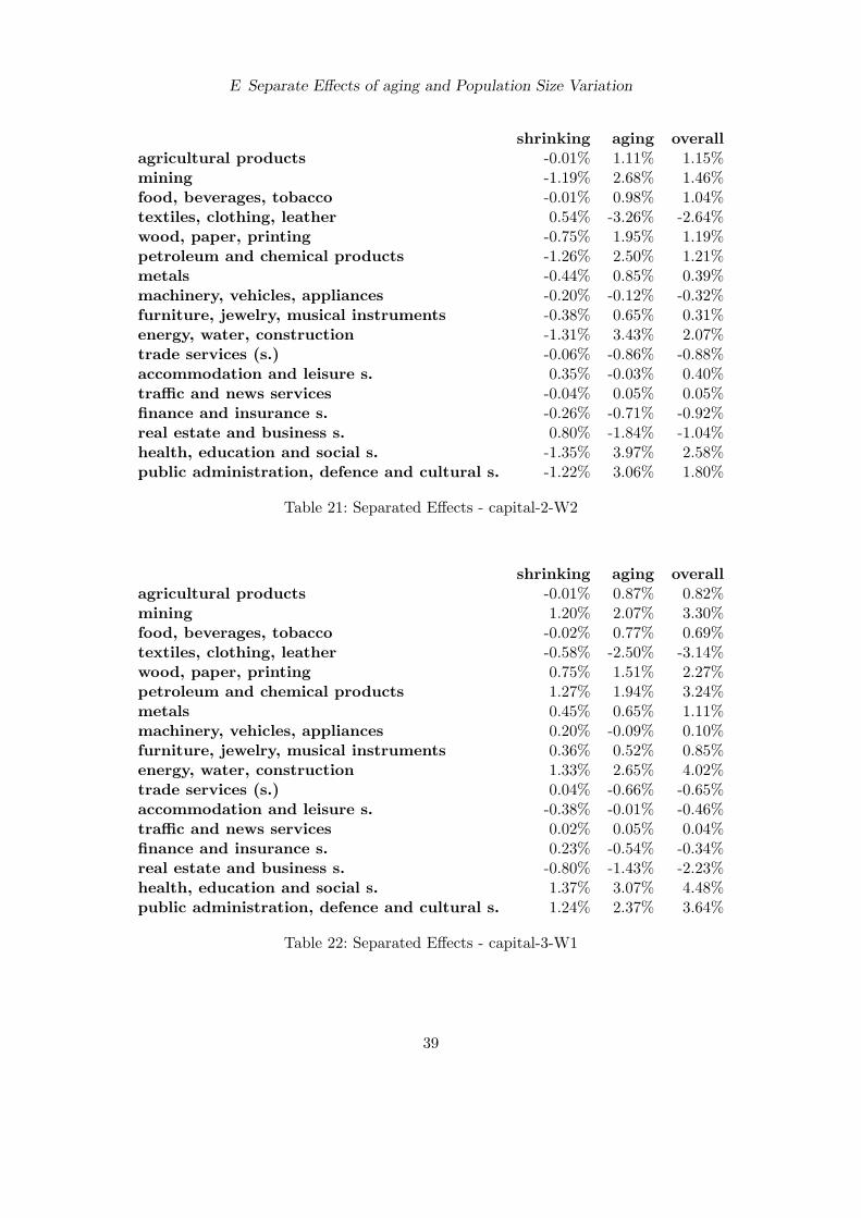
4.2 Separated effects
For clarification of the effect’s origin a separate look at the two main driving forces of thismodel is helpful. Comparative runs of modified versions of the model were undertakenin order to single out the effect of a change in population size and the effect of a changein age proportions. Thus, one modified model looked only at changes in population sizewhile holding the proportion of ‘active’ and ‘retired’ households fixed. In another modelmodification only the transition from ‘active’ to ‘retired’ households was considered butoverall population size kept constant. Tables 6-9 have been used above already for theoverall effects but should be considered again here for the separated effects. Exemplarily,for separability across the different population forecasts figures 7-10 show the change oflabor usage in the agricultural sector, production in the food, beverages and tobaccosector, exports in he public administration sector and in imports in the meals sector.A complete list of tables can be found in appendix E. Also price changes are shown inseparation in table 10. It emerges that the age effect dominates the size effect.
Price changes over the model horizonoriginal age size
agricultural products -5.8% -4.3% -1.8%mining -4.1% -3.0% -1.3%food, beverages, tobacco -5.1% -3.8% -1.6%textiles, clothing, leather -4.0% -2.9% -1.3%wood, paper, printing -5.0% -3.7% -1.6%petroleum and chemical products -4.5% -3.3% -1.4%metals -3.9% -2.9% -1.2%machinery, vehicles, appliances -3.6% -2.6% -1.1%furniture, jewelry, musical instruments -4.0% -3.0% -1.3%energy, water, construction -4.6% -3.4% -1.5%trade services -4.5% -3.3% -1.4%accommodation and leisure services -4.6% -3.4% -1.4%traffic and news services -5.0% -3.7% -1.6%finance and insurance services -4.6% -3.4% -1.5%real estate and business services -7.8% -5.8% -2.5%health, education and social services -3.7% -2.7% -1.2%public administration, defence and cultural services -3.9% -2.9% -1.2%
Table 10: Price changes over the model horizon - separate effects
15

4 Results
-20%
-15%
-10%
-5%
0%
5%
10%
1w1
1w2
2w1
2w2
3w1
3w2
4w1
4w2
5w1
5w2
6w1
6w2
shrinking ageing overall
Figure 7: labor usage in the agricultural sector - different scenarios
-12%
-10%
-8%
-6%
-4%
-2%
0%
2%
4%
6%
1w1
1w2
2w1
2w2
3w1
3w2
4w1
4w2
5w1
5w2
6w1
6w2
shrinking ageing overall
Figure 8: production in the food, beverages and tobacco sector
16

4 Results
-6%
-5%
-4%
-3%
-2%
-1%
0%
1%
2%
3%
1w1
1w2
2w1
2w2
3w1
3w2
4w1
4w2
5w1
5w2
6w1
6w2
shrinking ageing overall
Figure 9: exports in the public administration sector
-10%
-8%
-6%
-4%
-2%
0%
2%
4%
6%
1w1
1w2
2w1
2w2
3w1
3w2
4w1
4w2
5w1
5w2
6w1
6w2
shrinking ageing overall
Figure 10: imports in the metals sector
17

5 Conclusion
5 Conclusion
In contrast to many public finance papers, this paper has analyzed the sectoral effects ofthe projected demographic change in Germany using a computable general equilibriummodel calibrated to data for Germany with 17 production sectors and two householdtypes. It is based on the idea that the two main driving forces are a labor supply short-age accompanied by consumption demand changes both due to pronounced populationaging. The analysis is based on a static model with counterfactual runs for different pop-ulation forecasts. Thus there is leeway for further, dynamic research. Although frugalon dynamic complications and only including two household types the model is very de-tailed on the sectoral decomposition of the German economy. As there is a great degreeof interconnection between the sectors of an economy the consequences of an externalshock to the system cannot easily be predicted as there are too many forces interactingto allow a precise prediction of the outcome. Thus, the consequences for production andconsumption in the economy are worthwhile to be examined and found to be small butnon-negligible.
As is shown in section 4.1 the two changing factors, labor supply shortage and changingaggregate demand, affect the several sectors of the economy differently. Labor becomescomparably more expensive as the household type ‘active’ loses in number relatively.The sector reducing employment least is that of ‘health and education’.
Furthermore the ‘active’ households devote more and more of their disposable time tolabor. At the same time ‘retired’ households hold their amount of time devoted to laborabout constant.
All simulation results presented here are based on the assumption that aside fromadvanced population shrinking and aging there are no other changes in preferences,production technology or several shocks to the economy. This is certainly not a veryrealistic assumption but a model never makes the claim of reproducing every facet ofreality. It even seems advantageous to highlight only certain aspects and thus be able toidentify the effects more clearly.
Policy recommendations arising from these results might be a rise in legal retirementage, which would increase the pool of ‘working’ households and thus ease the pressurefrom labor supply shortage and at the same time probably also slow down the switch indemand preferences as it seems plausible that people change their demand depending onwhether they work and receive a normal wage or whether they are retired and receiveless money but at the same time have to meet different demands while in and out ofworking life. It seems not so much dependent on the actual age. (This assumes that theraise in retirement age is not too drastic.) One variant to a strict raise in legal retirementage could also be the introduction of part time retirement, leading to a ‘phasing out’- however, it needs to start at a later age than what is currently exercised. It mightalso be an indication for a necessary rethinking of the ‘pay-as-you-go’ system prevailingin Germany. An overall reduction of the utility level of the retired might be thinkable,though, for many not only non-desirable but also infeasible as it seems rather a long runsolution.
Investing in education thereby increasing the productivity of labor especially in those
18

5 Conclusion
sectors that will have a higher demand for labor due to the expected effects of populationaging can also be a beneficial policy. It is clear that demographic change will affect theGerman economy. Whether the effects will be severe and harmful to at least some groupsof the economy or not crucially depends on the policy environment.
19

References
References
Batini, N., T. Callen, and W. J. McKibbin (2006): “The Global Impact of Demo-graphic Change,” IMF Working Papers 06/9, International Monetary Fund.
Bloom, D. E., and D. Canning (2004): “Global Demographic Change : Dimensionsand Economic Significance,” Proceedings, (Aug), 9–56.
Bloom, D. E., and D. Canning (2006): “Global Demography: Fact, Force and Future,”in Demography and Financial Markets, ed. by C. Kent, A. Park, and D. Rees, RBAAnnual Conference Volume. Reserve Bank of Australia.
Bloom, D. E., D. Canning, G. Fink, and J. Finlay (2006): “Does Age StructureForecast Economic Growth?,” PGDA Working Papers 20, Program on the GlobalDemography of Aging.
Bloom, D. E., D. Canning, and P. N. Malaney (1999): “Demographic Changeand Economic Growth in Asia,” CID Working Papers 15, Center for InternationalDevelopment at Harvard University.
Boeters, S., C. Bohringer, T. Buttner, and M. Kraus (2006): “Economic Effectsof VAT Reform in Germany,” Discussion paper.
Boeters, S., R. Schnabel, and N. Gurtzgen (2006): “Reforming Social Welfare inGermany: An Applied General Equilibrium Analysis,” German Economic Review, 7,363–388.
Borsch-Supan, A. (2003): “Labor market effects of population aging,” Labour, 17(spe-cial issue), 5–44.
Bundesamt fur Bauwesen und Raumordnung (2005): “Raumordnungsprognose2020/2050,” Berichte, Band 23.
Denton, F. T., and B. G. Spencer (1999): “Population Aging and Its EconomicCosts: A Survey of the Issues and Evidence,” research paper no. 1, Social and EconomicDimensions of an Aging Population.
Deutsche Bundesbank (2004): “Demographische Belastungen fur Wachstum undWohlstand in Deutschland,” Monatsbericht, pp. 15–30.
Deutsches Institut fur Wirtschaftsforschung (2007): “Wachsende Bedeutungder Haushalte Alterer fur die Konsumnachfrage bis 2050,” Wochenbericht, DIWBerlin, (23), 361–366.
European Central Bank (2006): “Demographic change in the euro area: projectionsand consequences,” Monthly Bulletin, pp. 49–64.
20
References
Fougere, M., J. Mercener, and M. Merette (2007): “A sectoral and occupationalanalysis of population ageing in Canada using a dynamic CGE overlapping generationsmodel,” Economic Modelling, 24, 690–711.
Institut der deutschen Wirtschaft Koln (2007): Deutschland in Zahlen 2007.Deutscher Instituts-Verlag GmbH.
Kelley, A. C., and R. M. Schmidt (2001): “Economic and Demographic Change: ASynthesis of Models, Findings, and Perspectives,” in Population Does Matter: Demog-raphy, Growth, and Poverty in the Developing World, ed. by N. Birdsall, A. C. Kelley,and S. Sinding, pp. 67–105.
Klose, M., A. Opitz, and N. Schwarz (2005): “Sozialrechnungsmatrix 2000 -Konzepte und detaillierte Ergebnisse zu Einkommen, Konsum und Erwerbstatigkeit,”Band 6 der Schriftenreihe ’Sozio-okonomisches Berichtssystem fur eine nachhaltigeGesellschaft’.
Krueger, D., and A. Ludwig (2007): “On the consequences of demographic changefor rates of returns to capital, and the distribution of wealth and welfare,” Journal ofMonetary Economics, 54(1), 49–87.
Lehmann, H. (2004): “Auswirkungen demografischer Veranderungen auf Niveau undStruktur des Privaten Verbrauchs - eine Prognose fur Deutschland bis 2050,” Diskus-sionspapier 195, Institut fur Wirtschaftsforschung Halle (IWH).
Mathiesen, L. (1985): “Computation of economic equilibrium by a sequence of linear-complementarity problems,” Mathematical programming study 23, (North-Holland,Amsterdam).
Rutherford, T. F. (1995): “Extensions of GAMS for complementarity problems aris-ing in applied economics,” Journal of Economic Dynamics and Control, 19(8), 1299–1324.
Schaffnit-Chatterjee, C. (2007): “Wie werden altere Deutsche ihr Geld ausgeben?,”Aktuelle Themen 385, Deutsche Bank Research.
Statistisches Bundesamt (2006): Bevolkerung Deutschlands bis 2050, Ergebnisse der11. koordinierten Bevolkerungsvorausberechnung. Statistisches Bundesamt.
(2007): Entwicklung der Privathaushalte bis 2025, Ergebnisse der Haushaltsvo-rausberechnung 2007. Statistisches Bundesamt.
United Nations (2002): World population ageing 1950-2050. Retrieved Jan-uary 05, 2008 from http://www.un.org/esa/population/publications/worldageing19502050/index.htm.
United Nations, Department of Economic and Social Affairs, PopulationDivision (2006): Population Ageing 2006.
21

A Model Equations
AM
od
elE
qu
ati
on
s
A.1
mo
del
equ
ati
on
s
Inth
eco
mpl
emen
tari
tyfo
rmat
ther
ear
eth
ree
esse
ntia
ltyp
esof
equa
tion
s:ze
ropr
ofit
equa
tion
s,m
arke
tcl
eara
nce
equa
tion
san
din
com
eco
nstr
aint
s.
A.1
.1ze
rop
rofi
teq
ua
tio
ns
Zero
pro
fit
for
secto
rla
bor
supply
work
ing
Lwpleiw≥Lww
(1)
Zero
pro
fit
for
secto
rla
bor
supply
non-w
ork
ing
Lnplein≥Lnw
(2)
Zero
pro
fit
for
secto
ryi (L
i+Ki)w
Li
Li+Kir
Ki
Li+Ki
+∑ j
pa jintmedji
≥( tax
y i+
1) e i
px iθycet+
1
ei
+xdomi
+xdomipdom
iθycet+
1
ei
+xdomi
1
θycet+
1( e i
+xdomi
)(3
)
Zero
pro
fit
for
secto
rai
mipfxi
1−σa
mi
+xdomi
+xdomipdom
i1−σa
mi
+xdomi
1
1−σa( m i
+xdomi
) ≥aipa i
( taxa i
+1)
(4)
Zero
pro
fit
for
secto
rcow
(welf
are
work
ing) ( ∑
iCw ipa i1−σcow
Cw
)1
1−σcow
Cw
leisw
+Cw
pleis
w
leisw
leisw
+Cw( lei
sw
+Cw) ≥
pcw( lei
sw
+Cw)
(5)
22

A Model Equations
Zero
pro
fit
for
secto
rcon
(welf
are
non-w
ork
ing)
leisnpleis
n1−θcon
leisn
+Cn
+
Cn
( ∑iCn ipai1−σcon
Cn
)1
1−σcon
1−θcon
leisn
+Cn
11−θcon
( leisn
+Cn) ≥
pcn( lei
sn
+Cn)
(6)
Zero
pro
fit
for
secto
rgo
g0∏ i
pai
gd0i
g0≥pgg0
(7)
Zero
pro
fit
for
secto
rin
i0∏ i
pa i
id0i
i0≥pinvi0
(8)
Zero
pro
fit
for
secto
rexi
px iei≥pfxei
(9)
23

A Model Equations
A.1
.2m
arke
tcl
eara
nce
equ
ati
on
s
mark
et
cle
ara
nce
condit
ions
Supply
-dem
and
bala
nce
for
tim
e-
lab
or/
leis
ure
timew
+timen≥cow∗
( ∑iCw ipa(i
)1−σcow
Cw
)1
1−σcow
Cw
leisw
+Cw
leiswpleiw
leisw
leisw
+Cw−
1
leisw
+Cw
+tw∗Lw
+tn∗Ln
+con∗
leisn
leisnplein
1−θcon
leisn+Cn
+
Cn
( ∑iCn ipa(i
)1−σcon
Cn
)1
1−σcon
1−θcon
leisn+Cn
11−θcon−
1
(leisn
+Cn
)pleinθcon
(10)
Supply
-dem
and
bala
nce
for
com
modit
yxi
yi∗
eipx iθycet( tax
y i+
1) e i
px iθycet+
1
ei+xdomi
+xdomipdom
iθycet+
1
ei+xdomi
1
θycet+
1−
1
ei
+xdomi
≥ei∗
1
(11)
Supply
-dem
and
bala
nce
for
com
modit
ydi
yi∗
xdomipdom
iθycet( tax
y i+
1) e i
px iθycet+
1
ei+xdomi
+xdomipdom
iθycet+
1
ei+xdomi
1
θycet+
1−
1
ei
+xdomi
≥ai∗
xdomi
mipfx1−σa
mi+xdomi
+xdomipdom
i1−σa
mi+xdomi
1
1−σa−
1
( m i+xdomi
) pdom
iσa
(12)
Supply
-dem
and
bala
nce
for
dem
and
of
cw
cow∗
1≥leisw
+Cw
(13)
24

A Model Equations
Supply
-dem
and
bala
nce
for
dem
and
of
cn
con∗
1≥leisn
+Cn
(14)
Supply
-dem
and
bala
nce
for
dem
and
of
g
go∗
1≥g0
(15)
Supply
-dem
and
bala
nce
for
inv
in∗
1≥i0
(16)
Supply
-dem
and
bala
nce
forexi
ei∗
1≥ai∗
mi
mipfx1−σa
mi+xdomi
+xdomipdom
i1−σa
mi+xdomi
1
1−σa−
1
( m i+xdomi
) pfxσa
(17)
Supply
-dem
and
bala
nce
for
pri
mary
facto
rL
tw∗Lw
+tn∗Ln≥yi∗
Liw
Li
Li+Ki−
1r
Ki
Li+Ki
( ∑jintmedji
) +Li
+Ki
(18)
Supply
-dem
and
bala
nce
for
pri
mary
facto
rK
supply≥yi∗
Kiw
Li
Li+Kir
Ki
Li+Ki−
1
( ∑jintmedji
) +Li
+Ki
(19)
25

A Model Equations
A.1
.3in
com
eco
nst
rain
ts
incom
econst
rain
tsIn
com
edefi
nit
ion
for
house
hold
‘work
ing’/
‘young’
cow
=pleis
wtimew
+rcapw
+pfxbopdef
+pcwgovdef
+pinvi0−pcnlumptrans
(20)
Incom
edefi
nit
ion
for
house
hold
‘non-w
ork
ing’/
‘old
’
con
=pleis
ntimen
+rcapn
+pcnlumptrans
(21)
Incom
edefi
nit
ion
for
govern
ment
go
=( tax
a i+
1) a0
i+yi
(ed0i
+d0i)
ed0ipx ithetay+
1
ed0i
+d0i
+d0ipd ithetay+
1
ed0i
+d0i
1
thetay+
1(2
2)
26

A Model Equations
Variable definition
name definition
a0i initial Armington aggregate of sector i
ai Armington aggregate of sector i
bopdef balance of payments deficit
Cni ‘non-working’ household type’s sector i consumption
Cwi ‘working’ household type’s sector i consumption
Cn total consumption of household ‘non-working’
Cw total consumption of household ‘working’
con consumption of household ‘non-working’
cow consumption of household ‘working’
d0i initial home market final demand of sector i
ei export of sector i
ed0i initial export of sector i
g0 initial total government demand
gd0i initial government demand of sector i
go government demand
govdef government deficit
i0 total investment
id0i investment sector i
in investment
intmedji Armington aggregate of sector j used in sector i as intermediate
Ki capital used in sector i
leisn leisure consumed by household ‘old’/‘non-working’
leisw leisure consumed by household ‘young’/‘working’
Li labor used in sector i
Ln labor supplied by ‘old’ household
Lw labor supplied by ‘young’ household
mi import of sector i (to go into Armington)
r return on capital
lump trans lump sum transfer from working to non-working
timen initial time endowment ‘non-working’/‘old’ household
timew initial time endowment ‘working’/‘young’ household
tn time endowment ‘non-working’/‘old’ household
tw time endowment ‘working’/‘young’ household
w wage / return on labor
xdomiproduction of sector i used for domestic demand
yi production of sector i
...continued on next page
27

B Factor Intensities
...continued from page before
Variable definition
name definition
pg price of government consumption
pai price of (intermediate) Armington good of sector i
paj price of (intermediate) Armington good of sector j
pcn price of ‘non-working’ household’s consumption
pcw price of ‘working’ household’s consumption
pdomi price of good from sector i on domestic market
pxi price of good from sector i on foreign market
pfxi foreign price of import to sector i
pinv price of investment
pleisn price of leisure for household ‘old’/‘non-working’
pleisw price of leisure for household ‘young’/‘working’
pxi price of good xi
taxai tax on Armington good
taxyi tax on yi
θcon elasticity between leisure and goods consumption of household ‘old’
θycet elasticity of transformation on production process of yi
σa elasticity of Armington aggregate
σcon elasticity of household ‘non-working’/‘old’ in goods consumption
σcow elasticity of household ‘working’/‘young’ in goods consumption
B Factor Intensities
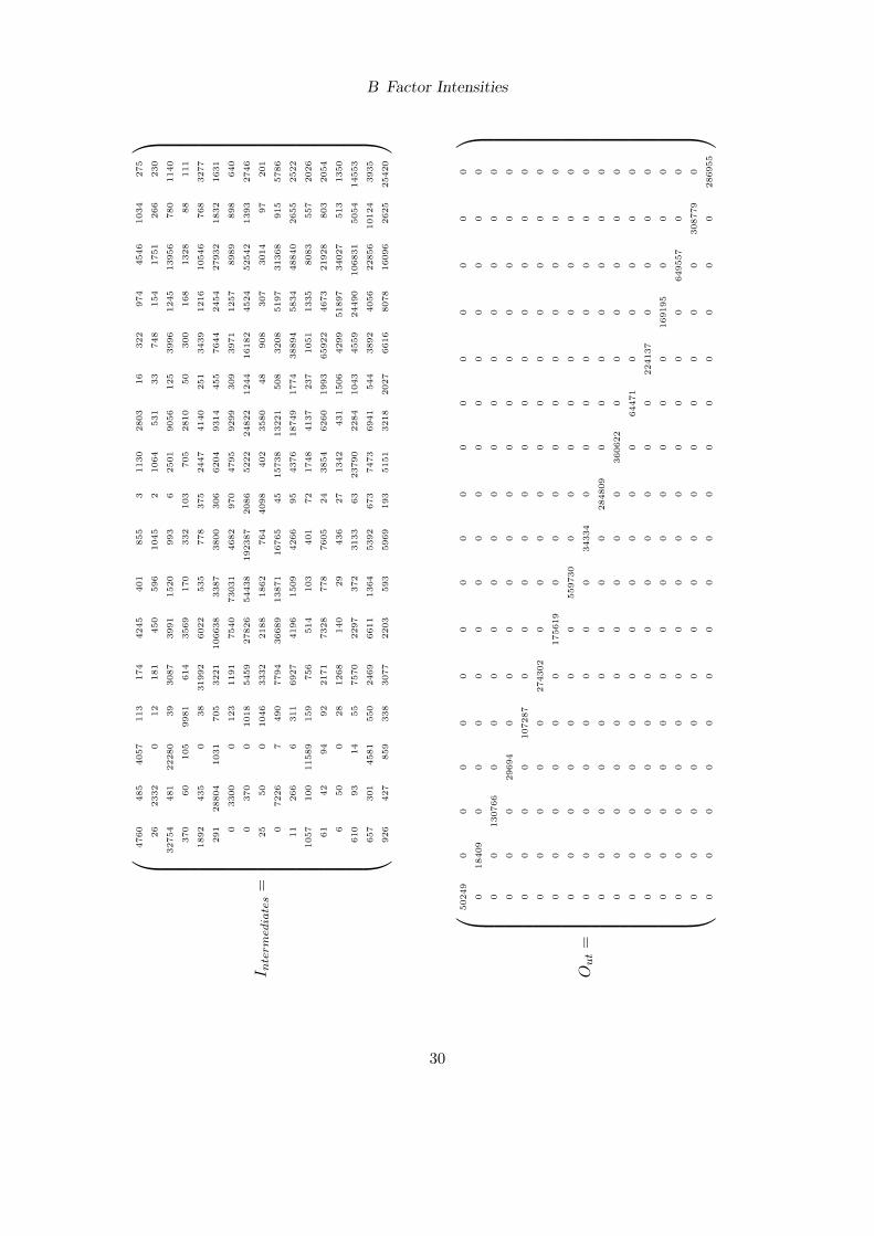
The calculation of the factor intensities for the individual sector follows the straightforward matrix algebra explained in this section. The calculations themselves were donewith a mathematical software package. Let Inter be the matrix of intermediate inputs(everything as price ∗ quantities), Sectors the vector of goods names, Factors the matrixof factors, Factornames the vector of factor names and Out the vector of outputs. Withthis, the following system can be set up to describe home production:
Intermediates ∗ Sectors + Factors ∗ Factornames = Out ∗ Sectors
Subtracting the right hand side and multiplying everything with the inverse of (Intermediates −Out)are the calculations needed to receive the result:
Sectors = − (Intermediates −Out)−1 ∗ Factors ∗ Factornames
28

B Factor Intensities
Giving the resulting matrix from the final calculation − (Intermediates −Out)−1∗Factors
the name Intensities all relevant matrices are:
S−1ectors = ( x1 x2 x3 x4 x5 x6 x7 x8 x9 x10 x11 x12 x13 x14 x15 x16 x17 )
F−1actornames = ( L K )
Intensities =
0.45167 0.548330.61523 0.384770.54064 0.459360.65925 0.340750.56484 0.435160.60965 0.390350.66015 0.339850.68293 0.317070.65197 0.348030.59807 0.401930.61575 0.384250.59834 0.401660.56909 0.430910.59906 0.400940.31559 0.684410.68278 0.317220.66613 0.33387
Factors =
8941 151155998 2990
21811 110056800 2030
23698 1543849801 1885240845 13779
142192 252799689 2723
80983 44998151477 6791421124 942259468 3898752677 19169
116132 336614166601 59759143423 59716
29
B Factor Intensities
I nte
rm
edia
tes
=
4760
485
4057
113
174
4245
401
855
31130
2803
16
322
974
4546
1034
275
26
2332
012
181
450
596
1045
21064
531
33
748
154
1751
266
230
32754
481
22280
39
3087
3991
1520
993
62501
9056
125
3996
1245
13956
780
1140
370
60
105
9981
614
3569
170
332
103
705
2810
50
300
168
1328
88
111
1892
435
038
31992
6022
535
778
375
2447
4140
251
3439
1216
10546
768
3277
291
28804
1031
705
3221
106638
3387
3800
306
6204
9314
455
7644
2454
27932
1832
1631
03300
0123
1191
7540
73031
4682
970
4795
9299
309
3971
1257
8989
898
640
0370
01018
5459
27826
54438
192387
2086
5222
24822
1244
16182
4524
52542
1393
2746
25
50
01046
3332
2188
1862
764
4098
402
3580
48
908
307
3014
97
201
07226
7490
7794
36689
13871
16765
45
15738
13221
508
3208
5197
31368
915
5786
11
266
6311
6927
4196
1509
4266
95
4376
18749
1774
38894
5834
48840
2655
2522
1057
100
11589
159
756
514
103
401
72
1748
4137
237
1051
1335
8083
557
2026
61
42
94
92
2171
7328
778
7605
24
3854
6260
1993
65922
4673
21928
803
2054
650
028
1268
140
29
436
27
1342
431
1506
4299
51897
34027
513
1350
610
93
14
55
7570
2297
372
3133
63
23790
2284
1043
4559
24490
106831
5054
14553
657
301
4581
550
2469
6611
1364
5392
673
7473
6941
544
3892
4056
22856
10124
3935
926
427
859
338
3077
2203
593
5969
193
5151
3218
2027
6616
8078
16096
2625
25420
Out
=
50249
00
00
00
00
00
00
00
00
018409
00
00
00
00
00
00
00
0
00
130766
00
00
00
00
00
00
00
00
029694
00
00
00
00
00
00
0
00
00
107287
00
00
00
00
00
00
00
00
0274302
00
00
00
00
00
0
00
00
00
175619
00
00
00
00
00
00
00
00
0559730
00
00
00
00
0
00
00
00
00
34334
00
00
00
00
00
00
00
00
0284809
00
00
00
0
00
00
00
00
00
360622
00
00
00
00
00
00
00
00
064471
00
00
0
00
00
00
00
00
00
224137
00
00
00
00
00
00
00
00
0169195
00
0
00
00
00
00
00
00
00
649557
00
00
00
00
00
00
00
00
0308779
0
00
00
00
00
00
00
00
00
286955
30

C Household Projection for the year 2050
C Household Projection for the year 2050
Official projections from the Statistisches Bundesamt for the number of households inGermany in the future according to age group and household type are only availableuntil the year 2025. Therefore own calculations were necessary to obtain projections forthe year 2050. Population projections for the year 2050 from Statistisches Bundesamt(2006) shown here in table 11 were combined with household members’ quotas for 2006to 2025 from Statistisches Bundesamt (2007). These quotas are shown in table 12.
German population in 2006 and 2050age from ... to under ...
0-5 5-10 10-15 15-20 20-25 25-30 30-35 35-40 40-45 45-502006 3498 3909 4039 4765 4841 4922 4793 6402 7215 65342050 variant 1-W1 2428 2500 2612 2825 3163 3502 3680 3720 3758 40122050 variant 1-W2 2703 2757 2862 3083 3486 3892 4093 4133 4168 44312050 variant 2-W1 2429 2500 2614 2825 3163 3503 3680 3721 3758 4012
age from ... to under ...50-55 55-60 60-65 65-70 70-75 75-80 80-85 85-90 90-95 95+
2006 5703 5110 4308 5459 3968 3063 2168 1075 411 1162050 variant 1-W1 4351 4406 4933 4634 4257 3926 4389 3419 1642 5932050 variant 1-W2 4773 4813 5282 4880 4422 4032 4451 3450 1654 5942050 variant 2-W1 4352 4413 4952 4679 4346 4091 4741 3916 2067 888
source: Statistisches Bundesamt (2006)
Table 11: Population projection for Germany for the year 2050
Population by age and household sizeage group 0-20 20-40household size 1 2 3 4 5+ 1 2 3 4 5+proportion 0.007 0.066 0.250 0.422 0.255 0.227 0.239 0.233 0.213 0.087individuals acc. to......variant 1-W1 72.6 684.1 2591.3 4374.0 2643.1 3192.8 3361.5 3277.2 2995.8 1223.7...variant 1-W2 79.8 752.7 2851.3 4812.9 2908.3 3542.1 3729.4 3635.7 3323.7 1357.5...variant 2-W1 72.6 684.3 2592.0 4375.3 2643.8 3193.2 3362.0 3277.6 2996.3 1223.8
age group 40-60 60+household size 1 2 3 4 5+ 1 2 3 4 5+proportion 0.159 0.353 0.232 0.186 0.070 0.301 0.606 0.066 0.016 0.010individuals acc. to......variant 1-W1 2627.8 5834.0 3834.3 3074.0 1156.9 8365.7 16842.6 1834.3 444.7 277.9...variant 1-W2 2891.4 6419.3 4218.9 3382.4 1273.0 8658.3 17431.6 1898.5 460.2 287.7...variant 2-W1 2629.1 5836.9 3836.1 3075.5 1157.5 8933.7 17986.1 1958.9 474.9 296.8
source: Statistisches Bundesamt (2007) and own calculations
Table 12: Household member projection for Germany for the year 2050
The quotas were taken from the status quo approach in the household members’ quotaapproach and used for own projections for the year 2050. Then, individuals were groupedinto households and households segmented according to ‘head of household’. This resultsin the numbers presented in table 13.
31

D Sensitivity Analysis
Projected household divisionworking age retired total
1-W1 16,202.84 19,045.19 35,248.021-W2 17,859.63 19,840.04 37,699.672-W1 16,234.22 20,212.01 36,446.22
Table 13: Projected household division
D Sensitivity Analysis
The discretionary choice that remains in the calibration process concerning parameterchoice calls for a critical examination. A comparison of the model as chosen and modeloutcomes given a different choice of parameters is necessary. This sensitivity analysisis undertaken to show that arbitrariness of results is excluded. This analysis is under-taken to test the results of the base model for robustness. The influence of the chosenparameters is evaluated via a systematic variation of the elasticities chosen. For all re-sulting combinations of different parameter values the model is evaluated and the resultsexamined.
This has been done for the base model and results have been found to be fairly robust.The ‘free’ parameters 10 are the following elasticities of the model:
θycet elasticity of transformation in production of yi
θyces elasticity of substitution in production of yi
θKL elasticity of primary factors in production of yi
σa Armington elasticityθcow elasticity of household ‘working’/‘young’ between leisure and goods consumptionσcow elasticity of household ‘working’/‘young’ in goods consumptionθcon elasticity of household ‘non-working’/‘old’ between leisure and goods consumptionσcon elasticity of household ‘non-working’/‘old’ in goods consumption
These parameters where changed to adopt values ranging from 0 to 8. In order todisplay this vast amount of data the results are shown for four parameters of the mode,namely labor used in the sectors, capital used in the sectors, production of each sectorand the behavior of prices. For each of those parameters results have been groupedaccording to the elasticities involved in the production process. Most representative forall results is in each of the following tables the colum named ‘1, 1, 1’ and it can be seen,that the results of this paper’s model are well within the bounds of these fluctuations.11
10‘Free’ because these parameters are not given by the social accounting matrix.11The values in the table mean that for the elasticities chosen in value as the name of the column
indicates, i.e. ‘1, 1, 1’ standing for θycet = 1, θyces = 1 and θKL = 1 the remaining elasticities wereallowed to vary between 0 and 8 in all possible combinations and the resulting model outcomes werein the range of the two values stated in the column.
32

D Sensitivity Analysis
deviation from benchmark: labormodel selected sensitivity runs
8, 8, 8 3, 3, 3 1, 1, 1 0.1, 0.1, 0.1 8, 3, 0
AGF -9.8% -9.7% -5.7% -0.8% 27.3% 7.7%-14.4% -14.3% -13.7% -14.0% -1.9%
MST -7.0% -8.4% -5.5% -3.3% -0.7% -4.2%-8.4% -11.6% -12.1% -13.9% -16.6%
FOP -10.0% -10.7% -7.0% -2.6% 2.8% -4.3%-14.8% -13.0% -14.7% -17.9% -18.9%
TXL -15.2% -13.8% -10.7% -6.9% -2.6% -9.1%-18.2% -19.6% -22.9% -35.4% -27.4%
PAP -8.3% -8.8% -6.1% -2.5% 1.8% -2.0%-12.1% -12.0% -11.9% -11.8% -10.3%
MIC -7.1% -8.5% -6.3% -3.5% 1.2% -5.1%-11.4% -11.5% -11.9% -11.1% -16.4%
MET -9.8% -7.3% -5.4% -3.0% -0.8% -4.6%-10.1% -10.8% -12.6% -23.6% -16.7%
MAC -11.1% -8.7% -7.3% -3.6% -1.3% -7.3%-8.7% -9.4% -15.5% -34.0% -24.0%
FUR -10.0% -9.8% -7.1% -3.9% -0.8% -6.5%-13.2% -13.7% -16.0% -20.9% -21.5%
EWC -6.2% -5.8% -4.0% -1.9% 0.1% -2.1%-7.9% -7.8% -7.5% -5.7% -8.1%
TRD -12.0% -11.3% -8.5% -5.2% -1.8% -6.1%-14.6% -14.9% -14.9% -17.8% -17.5%
HRI -11.5% -10.8% -7.5% -3.4% 0.6% -4.8%-14.8% -12.7% -16.4% -17.4% -18.8%
TRT -11.0% -10.1% -7.6% -3.8% -0.5% -3.8%-13.3% -9.6% -13.4% -12.6% -10.7%
BIN -11.7% -12.1% -9.2% -5.7% -2.1% -8.9%-15.4% -15.3% -15.2% -13.9% -21.4%
LIS -14.4% -9.9% -6.3% -2.2% 1.6% 13.0%-14.1% -14.0% -12.0% -5.9% 5.0%
HEA -4.3% -5.1% -3.9% -1.3% 0.2% -3.0%-7.3% -5.0% -8.1% -9.8% -8.6%
PBS -6.7% -6.3% -4.4% -2.3% -0.2% -3.5%-8.5% -8.6% -8.9% -7.4% -9.9%
Table 14: Sensitivity analysis (selected results for labor used)
33

D Sensitivity Analysis
deviation from benchmark: capitalmodel selected sensitivity runs
8, 8, 8 3, 3, 3 1, 1, 1 0.1, 0.1, 0.1 8, 3, 0
AGF 1.6% -0.5% 1.1% 5.4% 36.2% 8.8%-2.4% -2.7% -3.6% -10.2% -1.0%
MST 4.8% 1.2% 2.5% 2.6% 7.5% -3.7%0.4% -0.4% -3.0% -12.2% -15.8%
FOP 1.4% -1.5% -1.0% 1.1% 9.4% -4.0%-3.2% -2.1% -5.6% -14.9% -18.0%
TXL -4.4% -4.8% -4.1% -3.2% -1.6% -8.7%-7.2% -9.7% -15.5% -33.7% -26.7%
PAP 3.4% 0.7% 1.0% 3.0% 6.0% -1.6%0.0% -0.5% -2.4% -9.0% -9.5%
MIC 4.7% 1.5% 1.3% 3.0% 6.5% -4.7%0.3% -0.5% -2.7% -10.0% -15.5%
MET 1.7% 3.2% 3.2% 2.9% 0.3% -4.2%1.4% -0.1% -4.2% -18.3% -15.8%
MAC 0.2% 2.6% -1.3% 1.8% -0.5% -6.9%0.5% -1.3% -7.2% -29.5% -23.2%
FUR 1.4% -0.3% -0.3% -0.3% -0.3% -6.2%-1.6% -3.4% -7.7% -21.2% -20.8%
EWC 5.7% 3.7% 5.1% 4.9% 4.9% -1.7%3.7% 2.5% 1.3% -1.7% -7.0%
TRD -0.8% -2.0% -1.8% -1.4% -0.8% -5.6%-3.2% -4.5% -7.6% -15.3% -16.7%
HRI -0.3% -1.5% -1.5% 0.2% 1.5% -4.4%-3.3% -2.0% -7.7% -9.4% -18.1%
TRT 0.3% -0.8% -1.3% -0.3% 0.0% -3.5%-1.6% -1.3% -3.0% -2.5% -9.9%
BIN -0.5% -3.0% -2.6% -3.3% -1.1% -8.6%-3.8% -4.5% -3.3% -11.9% -20.8%
LIS -3.6% -0.8% 0.1% 1.7% 11.9% 13.7%-1.9% -1.9% -1.3% 0.0% 5.3%
HEA 7.9% 6.0% 2.6% 5.1% -0.6% -1.7%4.2% 2.6% 0.9% -7.7% -8.7%
PBS 5.2% 4.6% 4.6% 4.1% 3.5% -2.4%3.0% 1.7% 0.1% -4.8% -9.1%
Table 15: Sensitivity analysis (selected results for capital used)
34
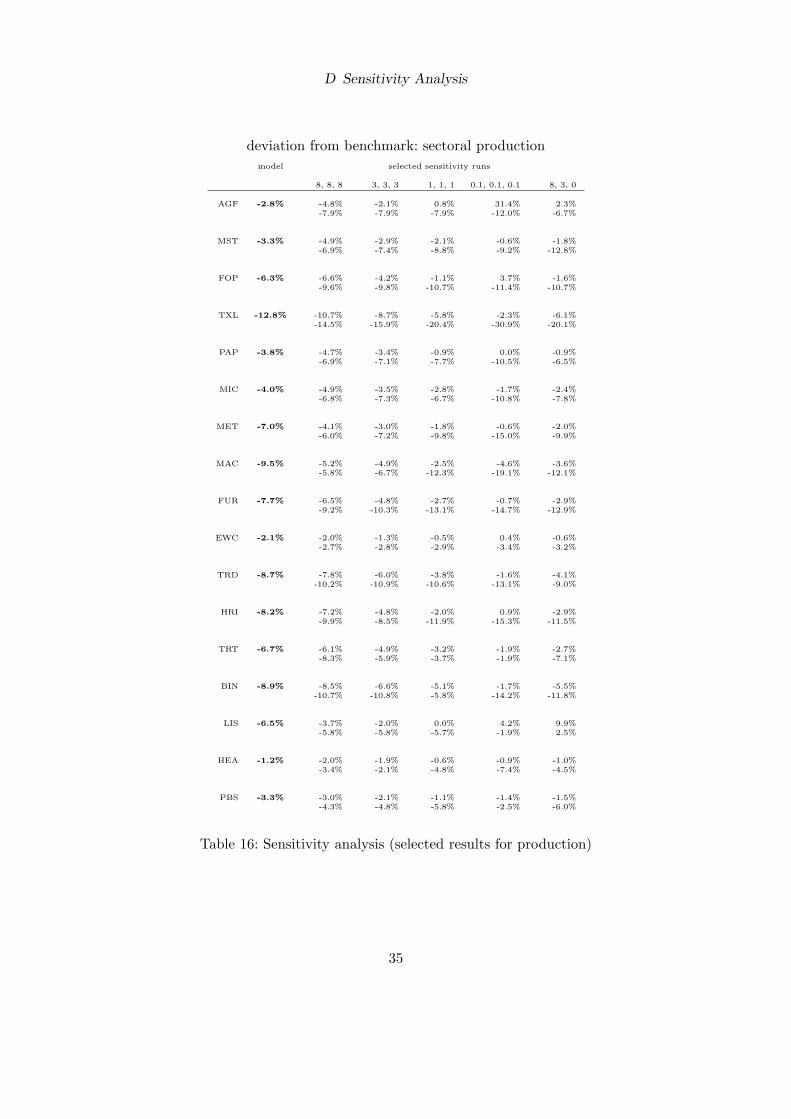
D Sensitivity Analysis
deviation from benchmark: sectoral productionmodel selected sensitivity runs
8, 8, 8 3, 3, 3 1, 1, 1 0.1, 0.1, 0.1 8, 3, 0
AGF -2.8% -4.8% -2.1% 0.8% 31.4% 2.3%-7.9% -7.9% -7.9% -12.0% -6.7%
MST -3.3% -4.9% -2.9% -2.1% -0.6% -1.8%-6.9% -7.4% -8.8% -9.2% -12.8%
FOP -6.3% -6.6% -4.2% -1.1% 3.7% -1.6%-9.6% -9.8% -10.7% -11.4% -10.7%
TXL -12.8% -10.7% -8.7% -5.8% -2.3% -6.1%-14.5% -15.9% -20.4% -30.9% -20.1%
PAP -3.8% -4.7% -3.4% -0.9% 0.0% -0.9%-6.9% -7.1% -7.7% -10.5% -6.5%
MIC -4.0% -4.9% -3.5% -2.8% -1.7% -2.4%-6.8% -7.3% -6.7% -10.8% -7.8%
MET -7.0% -4.1% -3.0% -1.8% -0.6% -2.0%-6.0% -7.2% -9.8% -15.0% -9.9%
MAC -9.5% -5.2% -4.9% -2.5% -4.6% -3.6%-5.8% -6.7% -12.3% -19.1% -12.1%
FUR -7.7% -6.5% -4.8% -2.7% -0.7% -2.9%-9.2% -10.3% -13.1% -14.7% -12.9%
EWC -2.1% -2.0% -1.3% -0.5% 0.4% -0.6%-2.7% -2.8% -2.9% -3.4% -3.2%
TRD -8.7% -7.8% -6.0% -3.8% -1.6% -4.1%-10.2% -10.9% -10.6% -13.1% -9.0%
HRI -8.2% -7.2% -4.8% -2.0% 0.9% -2.9%-9.9% -8.5% -11.9% -15.3% -11.5%
TRT -6.7% -6.1% -4.9% -3.2% -1.9% -2.7%-8.3% -5.9% -3.7% -1.9% -7.1%
BIN -8.9% -8.5% -6.6% -5.1% -1.7% -5.5%-10.7% -10.8% -5.8% -14.2% -11.8%
LIS -6.5% -3.7% -2.0% 0.0% 4.2% 9.9%-5.8% -5.8% -5.7% -1.9% 2.5%
HEA -1.2% -2.0% -1.9% -0.6% -0.9% -1.0%-3.4% -2.1% -4.8% -7.4% -4.5%
PBS -3.3% -3.0% -2.1% -1.1% -1.4% -1.5%-4.3% -4.8% -5.8% -2.5% -6.0%
Table 16: Sensitivity analysis (selected results for production)
35

D Sensitivity Analysis
deviation from benchmark: pricesmodel selected sensitivity runs
8, 8, 8 3, 3, 3 1, 1, 1 0.1, 0.1, 0.1 8, 3, 0
AGF -5.8% -0.6% -1.1% -1.6% -2.0% -1.6%-0.8% -2.2% -6.2% -32.9% -5.5%
MST -4.1% -0.4% -0.8% -1.1% -1.1% -0.9%-0.6% -1.6% -4.4% -23.0% -3.9%
FOP -5.1% -0.5% -1.0% -1.4% -1.8% -1.4%-0.7% -1.9% -5.5% -29.0% -4.8%
TXL -4.0% -0.4% -0.8% -1.1% -1.2% -1.0%-0.6% -1.5% -4.3% -22.3% -3.8%
PAP -5.0% -0.5% -1.0% -1.4% -1.8% -1.4%-0.7% -1.9% -5.4% -29.0% -4.8%
MIC -4.5% -0.5% -0.9% -1.3% -1.6% -1.2%-0.7% -1.7% -4.9% -25.8% -4.3%
MET -3.9% -0.4% -0.7% -1.1% -1.4% -1.1%-0.6% -1.5% -4.3% -22.8% -3.8%
MAC -3.6% -0.4% -0.7% -1.0% -1.3% -1.0%-0.5% -1.4% -3.9% -21.4% -3.8%
FUR -4.0% -0.4% -0.8% -1.1% -1.4% -1.1%-0.6% -1.5% -4.4% -23.1% -3.9%
EWC -4.6% -0.5% -0.9% -1.3% -1.7% -1.3%-0.7% -1.8% -5.0% -26.7% -4.5%
TRD -4.5% -0.5% -0.9% -1.3% -1.6% -1.2%-0.7% -1.7% -4.9% -26.3% -4.4%
HRI -4.6% -0.5% -0.9% -1.3% -1.7% -1.3%-0.7% -1.8% -5.0% -26.3% -4.4%
TRT -5.0% -0.5% -1.0% -1.4% -1.8% 0.0%-0.7% -1.9% -5.4% -28.9% -1.4%
BIN -4.6% -0.5% -0.9% -1.3% -1.7% -1.3%-0.7% -1.8% -5.0% -26.8% -4.5%
LIS -7.8% -0.8% -1.5% -2.2% -2.9% -2.2%-1.1% -3.0% -8.4% -45.2% -7.5%
HEA -3.7% -0.4% -0.7% -1.0% -1.3% -1.0%-0.5% -1.4% -4.0% -21.3% -3.5%
PBS -3.9% -0.4% -0.7% -1.1% -1.4% -1.1%-0.6% -1.5% -4.2% -22.4% -3.7%
Table 17: Sensitivity analysis (selected results for prices)
36

E Separate Effects of aging and Population Size Variation
E Separate Effects of aging and Population Size Variation
shrinking aging overallagricultural products -0.04% 1.11% 0.96%mining 2.48% 2.68% 5.22%food, beverages, tobacco -0.07% 0.98% 0.74%textiles, clothing, leather -1.22% -3.26% -4.65%wood, paper, printing 1.55% 1.95% 3.52%petroleum and chemical products 2.63% 2.50% 5.20%metals 0.92% 0.85% 1.79%machinery, vehicles, appliances 0.40% -0.12% 0.26%furniture, jewelry, musical instruments 0.73% 0.65% 1.29%energy, water, construction 2.75% 3.43% 6.29%trade services (s.) 0.06% -0.87% -0.89%accommodation and leisure s. -0.82% -0.03% -1.04%traffic and news services 0.02% 0.05% -0.01%finance and insurance s. 0.46% -0.71% -0.34%real estate and business s. -1.65% -1.85% -3.49%health, education and social s. 2.83% 3.98% 6.91%public administration, defence and cultural s. 2.57% 3.07% 5.72%
Table 18: Separated Effects - capital-1-W1
37

E Separate Effects of aging and Population Size Variation
shrinking aging overallagricultural products 0.00% 0.90% 0.90%mining -0.01% 2.15% 2.14%food, beverages, tobacco 0.00% 0.80% 0.80%textiles, clothing, leather 0.01% -2.61% -2.60%wood, paper, printing -0.01% 1.57% 1.56%petroleum and chemical products -0.02% 2.01% 2.00%metals -0.01% 0.68% 0.68%machinery, vehicles, appliances 0.00% -0.09% -0.10%furniture, jewelry, musical instruments 0.00% 0.53% 0.53%energy, water, construction -0.02% 2.76% 2.74%trade services (s.) 0.00% -0.69% -0.69%accommodation and leisure s. 0.00% -0.02% -0.01%traffic and news services 0.00% 0.05% 0.05%finance and insurance s. 0.00% -0.56% -0.56%real estate and business s. 0.01% -1.49% -1.48%health, education and social s. -0.02% 3.20% 3.18%public administration, defence and cultural s. -0.01% 2.46% 2.45%
Table 19: Separated Effects - capital-1-W2
shrinking aging overallagricultural products -0.01% 1.32% 1.24%mining 1.24% 3.22% 4.50%food, beverages, tobacco -0.02% 1.16% 1.04%textiles, clothing, leather -0.59% -3.95% -4.64%wood, paper, printing 0.77% 2.35% 3.13%petroleum and chemical products 1.31% 3.01% 4.36%metals 0.46% 1.02% 1.49%machinery, vehicles, appliances 0.20% -0.15% 0.04%furniture, jewelry, musical instruments 0.38% 0.77% 1.09%energy, water, construction 1.37% 4.14% 5.57%trade services (s.) 0.04% -1.06% -1.07%accommodation and leisure s. -0.39% -0.06% -0.56%traffic and news services 0.02% 0.05% 0.02%finance and insurance s. 0.24% -0.87% -0.69%real estate and business s. -0.83% -2.22% -3.04%health, education and social s. 1.41% 4.80% 6.26%public administration, defence and cultural s. 1.28% 3.69% 5.03%
Table 20: Separated Effects - capital-2-W1
38
E Separate Effects of aging and Population Size Variation
shrinking aging overallagricultural products -0.01% 1.11% 1.15%mining -1.19% 2.68% 1.46%food, beverages, tobacco -0.01% 0.98% 1.04%textiles, clothing, leather 0.54% -3.26% -2.64%wood, paper, printing -0.75% 1.95% 1.19%petroleum and chemical products -1.26% 2.50% 1.21%metals -0.44% 0.85% 0.39%machinery, vehicles, appliances -0.20% -0.12% -0.32%furniture, jewelry, musical instruments -0.38% 0.65% 0.31%energy, water, construction -1.31% 3.43% 2.07%trade services (s.) -0.06% -0.86% -0.88%accommodation and leisure s. 0.35% -0.03% 0.40%traffic and news services -0.04% 0.05% 0.05%finance and insurance s. -0.26% -0.71% -0.92%real estate and business s. 0.80% -1.84% -1.04%health, education and social s. -1.35% 3.97% 2.58%public administration, defence and cultural s. -1.22% 3.06% 1.80%
Table 21: Separated Effects - capital-2-W2
shrinking aging overallagricultural products -0.01% 0.87% 0.82%mining 1.20% 2.07% 3.30%food, beverages, tobacco -0.02% 0.77% 0.69%textiles, clothing, leather -0.58% -2.50% -3.14%wood, paper, printing 0.75% 1.51% 2.27%petroleum and chemical products 1.27% 1.94% 3.24%metals 0.45% 0.65% 1.11%machinery, vehicles, appliances 0.20% -0.09% 0.10%furniture, jewelry, musical instruments 0.36% 0.52% 0.85%energy, water, construction 1.33% 2.65% 4.02%trade services (s.) 0.04% -0.66% -0.65%accommodation and leisure s. -0.38% -0.01% -0.46%traffic and news services 0.02% 0.05% 0.04%finance and insurance s. 0.23% -0.54% -0.34%real estate and business s. -0.80% -1.43% -2.23%health, education and social s. 1.37% 3.07% 4.48%public administration, defence and cultural s. 1.24% 2.37% 3.64%
Table 22: Separated Effects - capital-3-W1
39

E Separate Effects of aging and Population Size Variation
shrinking aging overallagricultural products -0.02% 0.67% 0.69%mining -1.26% 1.58% 0.30%food, beverages, tobacco -0.01% 0.60% 0.63%textiles, clothing, leather 0.57% -1.90% -1.28%wood, paper, printing -0.80% 1.16% 0.35%petroleum and chemical products -1.34% 1.48% 0.12%metals -0.47% 0.50% 0.02%machinery, vehicles, appliances -0.22% -0.07% -0.28%furniture, jewelry, musical instruments -0.41% 0.40% 0.02%energy, water, construction -1.39% 2.02% 0.60%trade services (s.) -0.06% -0.50% -0.54%accommodation and leisure s. 0.37% 0.00% 0.42%traffic and news services -0.04% 0.04% 0.03%finance and insurance s. -0.27% -0.40% -0.65%real estate and business s. 0.85% -1.10% -0.24%health, education and social s. -1.43% 2.35% 0.88%public administration, defence and cultural s. -1.30% 1.81% 0.48%
Table 23: Separated Effects - capital-3-W2
shrinking aging overallagricultural products 0.00% 1.08% 1.08%mining 0.00% 2.60% 2.60%food, beverages, tobacco 0.00% 0.95% 0.95%textiles, clothing, leather 0.00% -3.17% -3.17%wood, paper, printing 0.00% 1.90% 1.90%petroleum and chemical products 0.00% 2.43% 2.43%metals 0.00% 0.82% 0.82%machinery, vehicles, appliances 0.00% -0.12% -0.12%furniture, jewelry, musical instruments 0.00% 0.64% 0.64%energy, water, construction 0.00% 3.33% 3.34%trade services (s.) 0.00% -0.84% -0.84%accommodation and leisure s. 0.00% -0.03% -0.03%traffic and news services 0.00% 0.05% 0.05%finance and insurance s. 0.00% -0.69% -0.69%real estate and business s. 0.00% -1.79% -1.79%health, education and social s. 0.00% 3.87% 3.87%public administration, defence and cultural s. 0.00% 2.98% 2.98%
Table 24: Separated Effects - capital-4-W1
40

E Separate Effects of aging and Population Size Variation
shrinking aging overallagricultural products -0.05% 0.87% 0.91%mining -2.39% 2.09% -0.35%food, beverages, tobacco -0.05% 0.78% 0.84%textiles, clothing, leather 1.05% -2.53% -1.35%wood, paper, printing -1.51% 1.53% 0.00%petroleum and chemical products -2.54% 1.96% -0.64%metals -0.90% 0.66% -0.25%machinery, vehicles, appliances -0.42% -0.09% -0.49%furniture, jewelry, musical instruments -0.79% 0.52% -0.21%energy, water, construction -2.63% 2.68% -0.03%trade services (s.) -0.14% -0.67% -0.74%accommodation and leisure s. 0.68% -0.01% 0.79%traffic and news services -0.09% 0.05% 0.02%finance and insurance s. -0.54% -0.54% -1.02%real estate and business s. 1.62% -1.45% 0.18%health, education and social s. -2.71% 3.11% 0.32%public administration, defence and cultural s. -2.46% 2.39% -0.14%
Table 25: Separated Effects - capital-4-W2
shrinking aging overallagricultural products -0.06% 1.24% 1.01%mining 3.17% 3.02% 6.28%food, beverages, tobacco -0.12% 1.09% 0.73%textiles, clothing, leather -1.59% -3.69% -5.53%wood, paper, printing 1.97% 2.20% 4.20%petroleum and chemical products 3.36% 2.82% 6.28%metals 1.18% 0.95% 2.16%machinery, vehicles, appliances 0.51% -0.14% 0.34%furniture, jewelry, musical instruments 0.92% 0.73% 1.51%energy, water, construction 3.52% 3.88% 7.55%trade services (s.) 0.06% -0.98% -1.05%accommodation and leisure s. -1.07% -0.05% -1.38%traffic and news services 0.02% 0.05% -0.05%finance and insurance s. 0.57% -0.81% -0.38%real estate and business s. -2.10% -2.08% -4.18%health, education and social s. 3.62% 4.49% 8.26%public administration, defence and cultural s. 3.28% 3.46% 6.87%
Table 26: Separated Effects - capital-5-W1
41
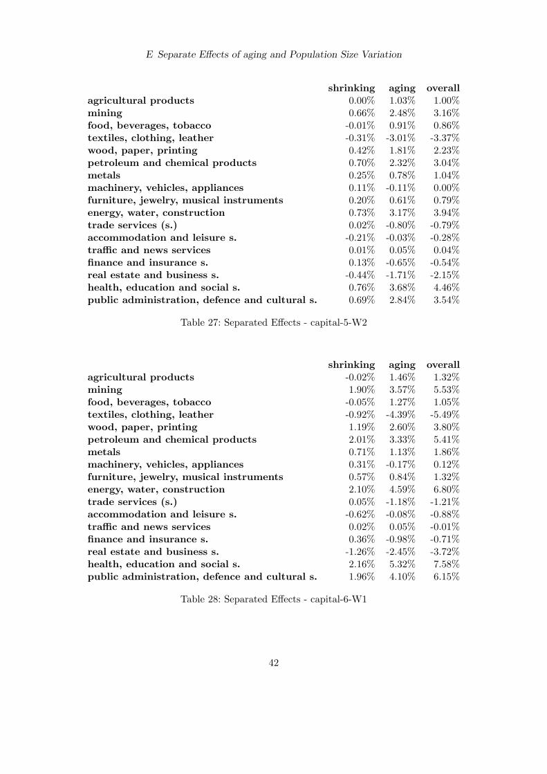
E Separate Effects of aging and Population Size Variation
shrinking aging overallagricultural products 0.00% 1.03% 1.00%mining 0.66% 2.48% 3.16%food, beverages, tobacco -0.01% 0.91% 0.86%textiles, clothing, leather -0.31% -3.01% -3.37%wood, paper, printing 0.42% 1.81% 2.23%petroleum and chemical products 0.70% 2.32% 3.04%metals 0.25% 0.78% 1.04%machinery, vehicles, appliances 0.11% -0.11% 0.00%furniture, jewelry, musical instruments 0.20% 0.61% 0.79%energy, water, construction 0.73% 3.17% 3.94%trade services (s.) 0.02% -0.80% -0.79%accommodation and leisure s. -0.21% -0.03% -0.28%traffic and news services 0.01% 0.05% 0.04%finance and insurance s. 0.13% -0.65% -0.54%real estate and business s. -0.44% -1.71% -2.15%health, education and social s. 0.76% 3.68% 4.46%public administration, defence and cultural s. 0.69% 2.84% 3.54%
Table 27: Separated Effects - capital-5-W2
shrinking aging overallagricultural products -0.02% 1.46% 1.32%mining 1.90% 3.57% 5.53%food, beverages, tobacco -0.05% 1.27% 1.05%textiles, clothing, leather -0.92% -4.39% -5.49%wood, paper, printing 1.19% 2.60% 3.80%petroleum and chemical products 2.01% 3.33% 5.41%metals 0.71% 1.13% 1.86%machinery, vehicles, appliances 0.31% -0.17% 0.12%furniture, jewelry, musical instruments 0.57% 0.84% 1.32%energy, water, construction 2.10% 4.59% 6.80%trade services (s.) 0.05% -1.18% -1.21%accommodation and leisure s. -0.62% -0.08% -0.88%traffic and news services 0.02% 0.05% -0.01%finance and insurance s. 0.36% -0.98% -0.71%real estate and business s. -1.26% -2.45% -3.72%health, education and social s. 2.16% 5.32% 7.58%public administration, defence and cultural s. 1.96% 4.10% 6.15%
Table 28: Separated Effects - capital-6-W1
42

E Separate Effects of aging and Population Size Variation
shrinking aging overallagricultural products 0.00% 1.24% 1.26%mining -0.53% 3.01% 2.46%food, beverages, tobacco 0.00% 1.09% 1.13%textiles, clothing, leather 0.25% -3.67% -3.39%wood, paper, printing -0.34% 2.19% 1.85%petroleum and chemical products -0.57% 2.81% 2.22%metals -0.20% 0.95% 0.74%machinery, vehicles, appliances -0.09% -0.14% -0.23%furniture, jewelry, musical instruments -0.17% 0.73% 0.58%energy, water, construction -0.59% 3.86% 3.24%trade services (s.) -0.02% -0.98% -0.98%accommodation and leisure s. 0.16% -0.05% 0.15%traffic and news services -0.01% 0.05% 0.06%finance and insurance s. -0.11% -0.81% -0.90%real estate and business s. 0.36% -2.07% -1.71%health, education and social s. -0.61% 4.47% 3.84%public administration, defence and cultural s. -0.55% 3.44% 2.87%
Table 29: Separated Effects - capital-6-W2
43

E Separate Effects of aging and Population Size Variation
shrinking aging overallagricultural products 1.32% 2.69% 3.93%mining -1.13% -1.38% -2.50%food, beverages, tobacco -2.41% -1.67% -4.19%textiles, clothing, leather -6.04% -8.56% -14.28%wood, paper, printing -0.64% -0.51% -1.15%petroleum and chemical products -1.25% -1.85% -3.09%metals -3.90% -4.57% -8.28%machinery, vehicles, appliances -5.47% -6.68% -11.82%furniture, jewelry, musical instruments -4.12% -4.79% -8.80%energy, water, construction -0.34% -0.06% -0.39%trade services (s.) -3.54% -4.86% -8.31%accommodation and leisure s. -4.16% -3.81% -7.98%traffic and news services -2.18% -2.42% -4.62%finance and insurance s. -3.13% -4.69% -7.77%real estate and business s. 3.18% 3.66% 6.92%public administration, defence and cultural s. -2.16% -2.27% -4.36%
Table 30: Separated Effects - exports-1-W1
shrinking aging overallagricultural products -0.01% 2.17% 2.16%mining 0.01% -1.11% -1.11%food, beverages, tobacco 0.01% -1.34% -1.32%textiles, clothing, leather 0.04% -6.93% -6.89%wood, paper, printing 0.00% -0.41% -0.40%petroleum and chemical products 0.01% -1.49% -1.48%metals 0.02% -3.69% -3.67%machinery, vehicles, appliances 0.03% -5.41% -5.38%furniture, jewelry, musical instruments 0.02% -3.87% -3.84%energy, water, construction 0.00% -0.05% -0.04%trade services (s.) 0.02% -3.93% -3.91%accommodation and leisure s. 0.02% -3.07% -3.04%traffic and news services 0.01% -1.94% -1.93%finance and insurance s. 0.02% -3.78% -3.76%real estate and business s. -0.02% 2.94% 2.92%public administration, defence and cultural s. 0.01% -1.83% -1.82%
Table 31: Separated Effects - exports-1-W2
44

E Separate Effects of aging and Population Size Variation
shrinking aging overallagricultural products 0.67% 3.23% 3.86%mining -0.57% -1.66% -2.22%food, beverages, tobacco -1.20% -2.02% -3.28%textiles, clothing, leather -3.05% -10.23% -13.09%wood, paper, printing -0.32% -0.61% -0.93%petroleum and chemical products -0.63% -2.22% -2.84%metals -1.98% -5.46% -7.32%machinery, vehicles, appliances -2.78% -7.97% -10.55%furniture, jewelry, musical instruments -2.08% -5.73% -7.75%energy, water, construction -0.17% -0.07% -0.24%trade services (s.) -1.78% -5.83% -7.55%accommodation and leisure s. -2.09% -4.57% -6.67%traffic and news services -1.09% -2.90% -4.01%finance and insurance s. -1.57% -5.62% -7.17%real estate and business s. 1.59% 4.40% 6.04%public administration, defence and cultural s. -1.09% -2.71% -3.77%
Table 32: Separated Effects - exports-2-W1
shrinking aging overallagricultural products -0.67% 2.69% 2.06%mining 0.56% -1.38% -0.83%food, beverages, tobacco 1.16% -1.67% -0.46%textiles, clothing, leather 3.02% -8.55% -5.69%wood, paper, printing 0.32% -0.51% -0.19%petroleum and chemical products 0.61% -1.85% -1.24%metals 1.96% -4.56% -2.69%machinery, vehicles, appliances 2.76% -6.67% -4.07%furniture, jewelry, musical instruments 2.04% -4.78% -2.79%energy, water, construction 0.17% -0.06% 0.11%trade services (s.) 1.74% -4.86% -3.16%accommodation and leisure s. 2.04% -3.80% -1.76%traffic and news services 1.06% -2.41% -1.34%finance and insurance s. 1.52% -4.68% -3.18%real estate and business s. -1.53% 3.65% 2.09%public administration, defence and cultural s. 1.08% -2.26% -1.22%
Table 33: Separated Effects - exports-2-W2
45

E Separate Effects of aging and Population Size Variation
shrinking aging overallagricultural products 0.65% 2.09% 2.71%mining -0.55% -1.07% -1.62%food, beverages, tobacco -1.17% -1.29% -2.49%textiles, clothing, leather -2.97% -6.67% -9.51%wood, paper, printing -0.31% -0.39% -0.71%petroleum and chemical products -0.61% -1.44% -2.04%metals -1.92% -3.56% -5.41%machinery, vehicles, appliances -2.70% -5.21% -7.78%furniture, jewelry, musical instruments -2.02% -3.72% -5.70%energy, water, construction -0.17% -0.05% -0.21%trade services (s.) -1.73% -3.78% -5.47%accommodation and leisure s. -2.03% -2.95% -4.99%traffic and news services -1.06% -1.87% -2.94%finance and insurance s. -1.52% -3.64% -5.15%real estate and business s. 1.54% 2.83% 4.40%public administration, defence and cultural s. -1.06% -1.76% -2.80%
Table 34: Separated Effects - exports-3-W1
shrinking aging overallagricultural products -0.71% 1.60% 0.91%mining 0.59% -0.82% -0.23%food, beverages, tobacco 1.23% -0.98% 0.28%textiles, clothing, leather 3.22% -5.13% -2.01%wood, paper, printing 0.34% -0.30% 0.04%petroleum and chemical products 0.65% -1.10% -0.45%metals 2.09% -2.74% -0.70%machinery, vehicles, appliances 2.95% -4.01% -1.17%furniture, jewelry, musical instruments 2.17% -2.86% -0.71%energy, water, construction 0.19% -0.04% 0.15%trade services (s.) 1.86% -2.90% -1.07%accommodation and leisure s. 2.17% -2.26% -0.08%traffic and news services 1.13% -1.43% -0.30%finance and insurance s. 1.62% -2.79% -1.18%real estate and business s. -1.62% 2.16% 0.51%public administration, defence and cultural s. 1.15% -1.35% -0.22%
Table 35: Separated Effects - exports-3-W2
46

E Separate Effects of aging and Population Size Variation
shrinking aging overallagricultural products 0.00% 2.62% 2.62%mining 0.00% -1.34% -1.34%food, beverages, tobacco 0.00% -1.62% -1.62%textiles, clothing, leather 0.00% -8.32% -8.33%wood, paper, printing 0.00% -0.49% -0.49%petroleum and chemical products 0.00% -1.80% -1.80%metals 0.00% -4.44% -4.44%machinery, vehicles, appliances 0.00% -6.50% -6.50%furniture, jewelry, musical instruments 0.00% -4.65% -4.66%energy, water, construction 0.00% -0.06% -0.06%trade services (s.) 0.00% -4.73% -4.73%accommodation and leisure s. 0.00% -3.70% -3.70%traffic and news services 0.00% -2.35% -2.35%finance and insurance s. 0.00% -4.56% -4.56%real estate and business s. 0.00% 3.55% 3.56%public administration, defence and cultural s. 0.00% -2.20% -2.20%
Table 36: Separated Effects - exports-4-W1
shrinking aging overallagricultural products -1.37% 2.11% 0.79%mining 1.13% -1.08% 0.04%food, beverages, tobacco 2.33% -1.30% 1.11%textiles, clothing, leather 6.17% -6.74% -0.83%wood, paper, printing 0.65% -0.40% 0.25%petroleum and chemical products 1.24% -1.45% -0.22%metals 4.01% -3.59% 0.28%machinery, vehicles, appliances 5.67% -5.26% 0.15%furniture, jewelry, musical instruments 4.16% -3.76% 0.32%energy, water, construction 0.36% -0.05% 0.31%trade services (s.) 3.54% -3.82% -0.35%accommodation and leisure s. 4.14% -2.98% 1.17%traffic and news services 2.15% -1.89% 0.27%finance and insurance s. 3.08% -3.68% -0.63%real estate and business s. -3.07% 2.86% -0.28%public administration, defence and cultural s. 2.20% -1.78% 0.37%
Table 37: Separated Effects - exports-4-W2
47

E Separate Effects of aging and Population Size Variation
shrinking aging overallagricultural products 1.67% 3.03% 4.58%mining -1.44% -1.55% -2.98%food, beverages, tobacco -3.09% -1.89% -5.13%textiles, clothing, leather -7.65% -9.62% -16.81%wood, paper, printing -0.82% -0.57% -1.39%petroleum and chemical products -1.59% -2.08% -3.65%metals -4.93% -5.13% -9.80%machinery, vehicles, appliances -6.92% -7.50% -13.95%furniture, jewelry, musical instruments -5.23% -5.38% -10.47%energy, water, construction -0.43% -0.06% -0.48%trade services (s.) -4.50% -5.47% -9.84%accommodation and leisure s. -5.29% -4.29% -9.59%traffic and news services -2.78% -2.72% -5.53%finance and insurance s. -3.98% -5.28% -9.20%real estate and business s. 4.07% 4.13% 8.31%public administration, defence and cultural s. -2.74% -2.55% -5.20%
Table 38: Separated Effects - exports-5-W1
shrinking aging overallagricultural products 0.36% 2.50% 2.84%mining -0.31% -1.28% -1.58%food, beverages, tobacco -0.65% -1.54% -2.22%textiles, clothing, leather -1.65% -7.94% -9.51%wood, paper, printing -0.18% -0.47% -0.64%petroleum and chemical products -0.34% -1.71% -2.05%metals -1.07% -4.23% -5.26%machinery, vehicles, appliances -1.51% -6.20% -7.62%furniture, jewelry, musical instruments -1.12% -4.44% -5.53%energy, water, construction -0.09% -0.05% -0.15%trade services (s.) -0.96% -4.51% -5.45%accommodation and leisure s. -1.13% -3.53% -4.66%traffic and news services -0.59% -2.24% -2.83%finance and insurance s. -0.85% -4.34% -5.18%real estate and business s. 0.85% 3.38% 4.26%public administration, defence and cultural s. -0.59% -2.10% -2.68%
Table 39: Separated Effects - exports-5-W2
48

E Separate Effects of aging and Population Size Variation
shrinking aging overallagricultural products 1.02% 3.57% 4.51%mining -0.87% -1.83% -2.69%food, beverages, tobacco -1.85% -2.24% -4.19%textiles, clothing, leather -4.65% -11.29% -15.61%wood, paper, printing -0.49% -0.67% -1.17%petroleum and chemical products -0.96% -2.46% -3.40%metals -3.00% -6.02% -8.84%machinery, vehicles, appliances -4.22% -8.79% -12.67%furniture, jewelry, musical instruments -3.17% -6.33% -9.40%energy, water, construction -0.26% -0.07% -0.33%trade services (s.) -2.72% -6.44% -9.06%accommodation and leisure s. -3.19% -5.06% -8.26%traffic and news services -1.67% -3.21% -4.91%finance and insurance s. -2.40% -6.22% -8.57%real estate and business s. 2.44% 4.88% 7.40%public administration, defence and cultural s. -1.66% -3.00% -4.60%
Table 40: Separated Effects - exports-6-W1
shrinking aging overallagricultural products -0.30% 3.02% 2.74%mining 0.25% -1.55% -1.30%food, beverages, tobacco 0.52% -1.88% -1.33%textiles, clothing, leather 1.35% -9.57% -8.30%wood, paper, printing 0.14% -0.57% -0.43%petroleum and chemical products 0.27% -2.07% -1.80%metals 0.87% -5.10% -4.27%machinery, vehicles, appliances 1.23% -7.46% -6.31%furniture, jewelry, musical instruments 0.91% -5.36% -4.47%energy, water, construction 0.08% -0.06% 0.01%trade services (s.) 0.78% -5.44% -4.69%accommodation and leisure s. 0.91% -4.27% -3.35%traffic and news services 0.48% -2.71% -2.23%finance and insurance s. 0.68% -5.25% -4.58%real estate and business s. -0.69% 4.11% 3.40%public administration, defence and cultural s. 0.48% -2.54% -2.07%
Table 41: Separated Effects - exports-6-W2
49

E Separate Effects of aging and Population Size Variation
shrinking aging overallagricultural products -2.37% -1.56% -4.00%mining -1.76% -2.12% -3.86%food, beverages, tobacco -4.20% -3.73% -7.92%textiles, clothing, leather -5.93% -8.46% -14.08%wood, paper, printing -2.28% -2.38% -4.62%petroleum and chemical products -1.98% -2.70% -4.63%metals -3.75% -4.42% -7.99%machinery, vehicles, appliances -4.86% -6.03% -10.61%furniture, jewelry, musical instruments -4.13% -4.83% -8.85%energy, water, construction -1.35% -1.23% -2.56%trade services (s.) -4.23% -5.66% -9.72%accommodation and leisure s. -5.07% -4.87% -9.87%traffic and news services -3.73% -4.19% -7.85%finance and insurance s. -4.10% -5.80% -9.75%real estate and business s. -3.23% -3.64% -6.79%health, education and social s. -1.85% -1.37% -3.21%public administration, defence and cultural s. -1.92% -2.02% -3.90%
Table 42: Separated Effects - production-1-W1
shrinking aging overallagricultural products 0.01% -1.25% -1.23%mining 0.01% -1.71% -1.70%food, beverages, tobacco 0.02% -3.00% -2.98%textiles, clothing, leather 0.04% -6.85% -6.81%wood, paper, printing 0.01% -1.92% -1.91%petroleum and chemical products 0.01% -2.18% -2.17%metals 0.02% -3.58% -3.56%machinery, vehicles, appliances 0.03% -4.88% -4.85%furniture, jewelry, musical instruments 0.02% -3.90% -3.88%energy, water, construction 0.01% -0.99% -0.98%trade services (s.) 0.03% -4.57% -4.55%accommodation and leisure s. 0.03% -3.93% -3.90%traffic and news services 0.02% -3.39% -3.36%finance and insurance s. 0.02% -4.69% -4.66%real estate and business s. 0.02% -2.94% -2.92%health, education and social s. 0.01% -1.10% -1.09%public administration, defence and cultural s. 0.01% -1.64% -1.62%
Table 43: Separated Effects - production-1-W2
50

E Separate Effects of aging and Population Size Variation
shrinking aging overallagricultural products -1.18% -1.88% -3.11%mining -0.89% -2.54% -3.41%food, beverages, tobacco -2.11% -4.47% -6.59%textiles, clothing, leather -3.00% -10.12% -12.93%wood, paper, printing -1.15% -2.86% -3.98%petroleum and chemical products -1.00% -3.23% -4.20%metals -1.90% -5.28% -7.08%machinery, vehicles, appliances -2.47% -7.20% -9.50%furniture, jewelry, musical instruments -2.09% -5.78% -7.80%energy, water, construction -0.68% -1.47% -2.14%trade services (s.) -2.13% -6.77% -8.81%accommodation and leisure s. -2.56% -5.84% -8.35%traffic and news services -1.88% -5.02% -6.86%finance and insurance s. -2.07% -6.94% -8.92%real estate and business s. -1.63% -4.36% -5.94%health, education and social s. -0.94% -1.64% -2.57%public administration, defence and cultural s. -0.97% -2.43% -3.37%
Table 44: Separated Effects - production-2-W1
shrinking aging overallagricultural products 1.14% -1.55% -0.37%mining 0.87% -2.12% -1.26%food, beverages, tobacco 2.06% -3.72% -1.66%textiles, clothing, leather 2.96% -8.45% -5.65%wood, paper, printing 1.13% -2.38% -1.27%petroleum and chemical products 0.98% -2.69% -1.74%metals 1.88% -4.42% -2.62%machinery, vehicles, appliances 2.45% -6.02% -3.70%furniture, jewelry, musical instruments 2.05% -4.82% -2.83%energy, water, construction 0.67% -1.23% -0.57%trade services (s.) 2.10% -5.65% -3.63%accommodation and leisure s. 2.52% -4.87% -2.39%traffic and news services 1.85% -4.19% -2.38%finance and insurance s. 2.03% -5.79% -3.84%real estate and business s. 1.60% -3.63% -2.07%health, education and social s. 0.92% -1.37% -0.45%public administration, defence and cultural s. 0.95% -2.02% -1.09%
Table 45: Separated Effects - production-2-W2
51

E Separate Effects of aging and Population Size Variation
shrinking aging overallagricultural products -1.15% -1.20% -2.38%mining -0.86% -1.65% -2.50%food, beverages, tobacco -2.05% -2.89% -4.94%textiles, clothing, leather -2.91% -6.59% -9.39%wood, paper, printing -1.11% -1.85% -2.95%petroleum and chemical products -0.97% -2.10% -3.05%metals -1.84% -3.45% -5.22%machinery, vehicles, appliances -2.39% -4.70% -6.99%furniture, jewelry, musical instruments -2.03% -3.76% -5.74%energy, water, construction -0.66% -0.96% -1.61%trade services (s.) -2.07% -4.40% -6.41%accommodation and leisure s. -2.49% -3.79% -6.24%traffic and news services -1.83% -3.26% -5.06%finance and insurance s. -2.01% -4.51% -6.46%real estate and business s. -1.58% -2.83% -4.38%health, education and social s. -0.91% -1.06% -1.97%public administration, defence and cultural s. -0.94% -1.57% -2.50%
Table 46: Separated Effects - production-3-W1
shrinking aging overallagricultural products 1.21% -0.92% 0.33%mining 0.93% -1.26% -0.34%food, beverages, tobacco 2.20% -2.21% -0.01%textiles, clothing, leather 3.15% -5.07% -2.01%wood, paper, printing 1.20% -1.42% -0.23%petroleum and chemical products 1.04% -1.61% -0.58%metals 2.01% -2.65% -0.70%machinery, vehicles, appliances 2.61% -3.62% -1.09%furniture, jewelry, musical instruments 2.18% -2.88% -0.73%energy, water, construction 0.72% -0.73% -0.02%trade services (s.) 2.23% -3.38% -1.20%accommodation and leisure s. 2.68% -2.90% -0.24%traffic and news services 1.97% -2.50% -0.56%finance and insurance s. 2.16% -3.47% -1.35%real estate and business s. 1.71% -2.17% -0.49%health, education and social s. 0.98% -0.81% 0.17%public administration, defence and cultural s. 1.02% -1.21% -0.21%
Table 47: Separated Effects - production-3-W2
52

E Separate Effects of aging and Population Size Variation
shrinking aging overallagricultural products 0.00% -1.51% -1.51%mining 0.00% -2.06% -2.06%food, beverages, tobacco 0.00% -3.62% -3.62%textiles, clothing, leather 0.00% -8.23% -8.23%wood, paper, printing 0.00% -2.32% -2.32%petroleum and chemical products 0.00% -2.62% -2.62%metals 0.00% -4.30% -4.30%machinery, vehicles, appliances 0.00% -5.86% -5.86%furniture, jewelry, musical instruments 0.00% -4.69% -4.70%energy, water, construction 0.00% -1.20% -1.20%trade services (s.) 0.00% -5.50% -5.50%accommodation and leisure s. 0.00% -4.74% -4.74%traffic and news services 0.00% -4.08% -4.08%finance and insurance s. 0.00% -5.64% -5.64%real estate and business s. 0.00% -3.54% -3.54%health, education and social s. 0.00% -1.33% -1.33%public administration, defence and cultural s. 0.00% -1.97% -1.97%
Table 48: Separated Effects - production-4-W1
shrinking aging overallagricultural products 2.30% -1.21% 1.16%mining 1.77% -1.66% 0.09%food, beverages, tobacco 4.19% -2.92% 1.28%textiles, clothing, leather 6.05% -6.66% -0.86%wood, paper, printing 2.29% -1.87% 0.39%petroleum and chemical products 1.99% -2.12% -0.17%metals 3.85% -3.48% 0.24%machinery, vehicles, appliances 5.02% -4.75% 0.06%furniture, jewelry, musical instruments 4.18% -3.79% 0.30%energy, water, construction 1.37% -0.97% 0.39%trade services (s.) 4.27% -4.45% -0.30%accommodation and leisure s. 5.13% -3.82% 1.25%traffic and news services 3.76% -3.29% 0.41%finance and insurance s. 4.13% -4.56% -0.54%real estate and business s. 3.27% -2.86% 0.35%health, education and social s. 1.88% -1.07% 0.80%public administration, defence and cultural s. 1.95% -1.59% 0.32%
Table 49: Separated Effects - production-4-W2
53

E Separate Effects of aging and Population Size Variation
shrinking aging overallagricultural products -3.02% -1.76% -4.89%mining -2.24% -2.39% -4.59%food, beverages, tobacco -5.34% -4.20% -9.53%textiles, clothing, leather -7.51% -9.50% -16.58%wood, paper, printing -2.89% -2.68% -5.52%petroleum and chemical products -2.52% -3.03% -5.48%metals -4.74% -4.97% -9.46%machinery, vehicles, appliances -6.15% -6.76% -12.52%furniture, jewelry, musical instruments -5.24% -5.43% -10.51%energy, water, construction -1.71% -1.38% -3.06%trade services (s.) -5.36% -6.36% -11.49%accommodation and leisure s. -6.44% -5.48% -11.81%traffic and news services -4.74% -4.72% -9.34%finance and insurance s. -5.21% -6.52% -11.51%real estate and business s. -4.11% -4.09% -8.08%health, education and social s. -2.35% -1.54% -3.88%public administration, defence and cultural s. -2.44% -2.28% -4.65%
Table 50: Separated Effects - production-5-W1
shrinking aging overallagricultural products -0.64% -1.44% -2.10%mining -0.48% -1.97% -2.44%food, beverages, tobacco -1.14% -3.45% -4.59%textiles, clothing, leather -1.62% -7.85% -9.39%wood, paper, printing -0.62% -2.21% -2.82%petroleum and chemical products -0.54% -2.50% -3.03%metals -1.03% -4.10% -5.09%machinery, vehicles, appliances -1.34% -5.59% -6.86%furniture, jewelry, musical instruments -1.13% -4.48% -5.58%energy, water, construction -0.37% -1.14% -1.50%trade services (s.) -1.15% -5.25% -6.36%accommodation and leisure s. -1.38% -4.52% -5.88%traffic and news services -1.02% -3.89% -4.88%finance and insurance s. -1.12% -5.38% -6.46%real estate and business s. -0.88% -3.37% -4.24%health, education and social s. -0.51% -1.27% -1.77%public administration, defence and cultural s. -0.52% -1.88% -2.39%
Table 51: Separated Effects - production-5-W2
54

E Separate Effects of aging and Population Size Variation
shrinking aging overallagricultural products -1.81% -2.08% -3.98%mining -1.36% -2.81% -4.14%food, beverages, tobacco -3.22% -4.95% -8.17%textiles, clothing, leather -4.56% -11.16% -15.41%wood, paper, printing -1.75% -3.16% -4.87%petroleum and chemical products -1.52% -3.57% -5.04%metals -2.89% -5.83% -8.54%machinery, vehicles, appliances -3.75% -7.93% -11.40%furniture, jewelry, musical instruments -3.18% -6.39% -9.45%energy, water, construction -1.04% -1.63% -2.64%trade services (s.) -3.25% -7.47% -10.56%accommodation and leisure s. -3.90% -6.45% -10.28%traffic and news services -2.87% -5.55% -8.34%finance and insurance s. -3.15% -7.66% -10.66%real estate and business s. -2.49% -4.81% -7.22%health, education and social s. -1.43% -1.82% -3.23%public administration, defence and cultural s. -1.48% -2.68% -4.11%
Table 52: Separated Effects - production-6-W1
shrinking aging overallagricultural products 0.51% -1.75% -1.22%mining 0.39% -2.38% -1.99%food, beverages, tobacco 0.92% -4.18% -3.25%textiles, clothing, leather 1.32% -9.46% -8.22%wood, paper, printing 0.50% -2.67% -2.17%petroleum and chemical products 0.44% -3.02% -2.59%metals 0.84% -4.94% -4.15%machinery, vehicles, appliances 1.09% -6.73% -5.71%furniture, jewelry, musical instruments 0.92% -5.40% -4.52%energy, water, construction 0.30% -1.38% -1.08%trade services (s.) 0.94% -6.33% -5.43%accommodation and leisure s. 1.12% -5.46% -4.35%traffic and news services 0.83% -4.69% -3.89%finance and insurance s. 0.91% -6.49% -5.62%real estate and business s. 0.72% -4.07% -3.37%health, education and social s. 0.41% -1.53% -1.12%public administration, defence and cultural s. 0.43% -2.27% -1.85%
Table 53: Separated Effects - production-6-W2
55

E Separate Effects of aging and Population Size Variation
shrinking aging overallagricultural products -6.80% -6.63% -13.14%mining -2.60% -3.10% -5.63%food, beverages, tobacco -6.71% -6.62% -13.08%textiles, clothing, leather -5.29% -7.88% -12.93%wood, paper, printing -4.89% -5.38% -10.07%petroleum and chemical products -3.60% -4.57% -8.01%metals -3.47% -4.16% -7.46%machinery, vehicles, appliances -2.58% -3.58% -6.04%furniture, jewelry, musical instruments -4.16% -4.91% -8.93%energy, water, construction -2.35% -2.39% -4.68%trade services (s.) -5.06% -6.62% -11.43%accommodation and leisure s. -6.09% -6.06% -11.94%traffic and news services -5.67% -6.41% -11.81%finance and insurance s. -5.17% -7.01% -11.88%real estate and business s. -9.69% -10.91% -19.61%health, education and social s. -1.30% -0.76% -2.07%public administration, defence and cultural s. -1.68% -1.78% -3.43%
Table 54: Separated Effects - imports-1-W1
shrinking aging overallagricultural products 0.04% -5.37% -5.33%mining 0.02% -2.51% -2.49%food, beverages, tobacco 0.04% -5.36% -5.32%textiles, clothing, leather 0.03% -6.37% -6.34%wood, paper, printing 0.03% -4.35% -4.33%petroleum and chemical products 0.02% -3.70% -3.67%metals 0.02% -3.36% -3.34%machinery, vehicles, appliances 0.02% -2.90% -2.88%furniture, jewelry, musical instruments 0.02% -3.97% -3.94%energy, water, construction 0.01% -1.93% -1.92%trade services (s.) 0.03% -5.36% -5.33%accommodation and leisure s. 0.04% -4.90% -4.86%traffic and news services 0.03% -5.19% -5.16%finance and insurance s. 0.03% -5.68% -5.65%real estate and business s. 0.06% -8.88% -8.83%health, education and social s. 0.01% -0.62% -0.61%public administration, defence and cultural s. 0.01% -1.44% -1.43%
Table 55: Separated Effects - imports-1-W2
56

E Separate Effects of aging and Population Size Variation
shrinking aging overallagricultural products -3.45% -7.93% -11.21%mining -1.31% -3.71% -4.99%food, beverages, tobacco -3.40% -7.92% -11.17%textiles, clothing, leather -2.67% -9.43% -11.95%wood, paper, printing -2.48% -6.43% -8.79%petroleum and chemical products -1.82% -5.46% -7.18%metals -1.76% -4.97% -6.62%machinery, vehicles, appliances -1.31% -4.28% -5.51%furniture, jewelry, musical instruments -2.10% -5.87% -7.89%energy, water, construction -1.19% -2.87% -4.02%trade services (s.) -2.56% -7.91% -10.32%accommodation and leisure s. -3.09% -7.24% -10.21%traffic and news services -2.88% -7.66% -10.37%finance and insurance s. -2.62% -8.38% -10.81%real estate and business s. -4.97% -12.96% -17.34%health, education and social s. -0.65% -0.92% -1.58%public administration, defence and cultural s. -0.85% -2.13% -2.96%
Table 56: Separated Effects - imports-2-W1
shrinking aging overallagricultural products 3.44% -6.63% -3.33%mining 1.29% -3.10% -1.84%food, beverages, tobacco 3.38% -6.61% -3.36%textiles, clothing, leather 2.63% -7.87% -5.37%wood, paper, printing 2.45% -5.38% -3.02%petroleum and chemical products 1.80% -4.56% -2.84%metals 1.74% -4.15% -2.49%machinery, vehicles, appliances 1.29% -3.58% -2.35%furniture, jewelry, musical instruments 2.07% -4.90% -2.90%energy, water, construction 1.17% -2.39% -1.25%trade services (s.) 2.53% -6.62% -4.21%accommodation and leisure s. 3.05% -6.05% -3.09%traffic and news services 2.86% -6.41% -3.68%finance and insurance s. 2.59% -7.01% -4.56%real estate and business s. 5.06% -10.90% -6.34%health, education and social s. 0.64% -0.76% -0.12%public administration, defence and cultural s. 0.83% -1.78% -0.96%
Table 57: Separated Effects - imports-2-W2
57
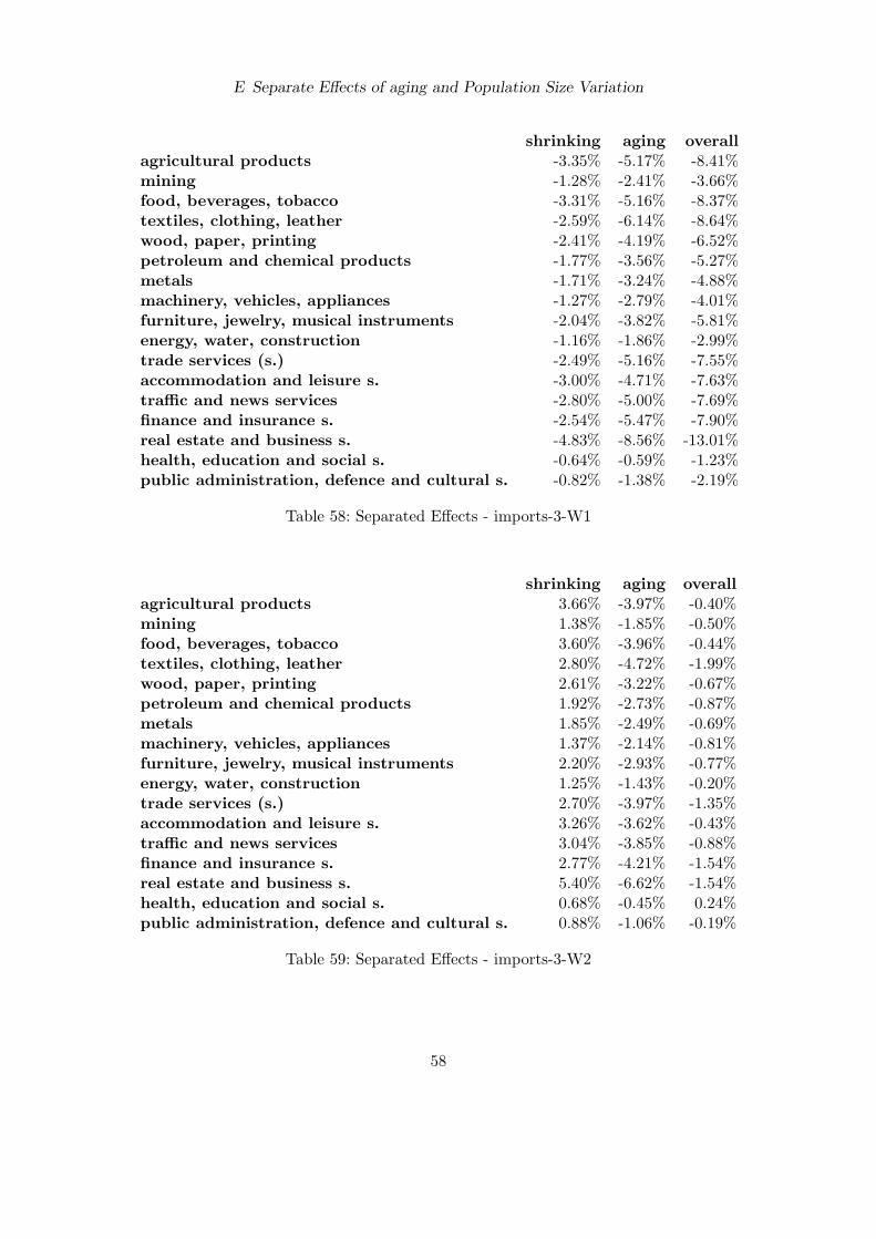
E Separate Effects of aging and Population Size Variation
shrinking aging overallagricultural products -3.35% -5.17% -8.41%mining -1.28% -2.41% -3.66%food, beverages, tobacco -3.31% -5.16% -8.37%textiles, clothing, leather -2.59% -6.14% -8.64%wood, paper, printing -2.41% -4.19% -6.52%petroleum and chemical products -1.77% -3.56% -5.27%metals -1.71% -3.24% -4.88%machinery, vehicles, appliances -1.27% -2.79% -4.01%furniture, jewelry, musical instruments -2.04% -3.82% -5.81%energy, water, construction -1.16% -1.86% -2.99%trade services (s.) -2.49% -5.16% -7.55%accommodation and leisure s. -3.00% -4.71% -7.63%traffic and news services -2.80% -5.00% -7.69%finance and insurance s. -2.54% -5.47% -7.90%real estate and business s. -4.83% -8.56% -13.01%health, education and social s. -0.64% -0.59% -1.23%public administration, defence and cultural s. -0.82% -1.38% -2.19%
Table 58: Separated Effects - imports-3-W1
shrinking aging overallagricultural products 3.66% -3.97% -0.40%mining 1.38% -1.85% -0.50%food, beverages, tobacco 3.60% -3.96% -0.44%textiles, clothing, leather 2.80% -4.72% -1.99%wood, paper, printing 2.61% -3.22% -0.67%petroleum and chemical products 1.92% -2.73% -0.87%metals 1.85% -2.49% -0.69%machinery, vehicles, appliances 1.37% -2.14% -0.81%furniture, jewelry, musical instruments 2.20% -2.93% -0.77%energy, water, construction 1.25% -1.43% -0.20%trade services (s.) 2.70% -3.97% -1.35%accommodation and leisure s. 3.26% -3.62% -0.43%traffic and news services 3.04% -3.85% -0.88%finance and insurance s. 2.77% -4.21% -1.54%real estate and business s. 5.40% -6.62% -1.54%health, education and social s. 0.68% -0.45% 0.24%public administration, defence and cultural s. 0.88% -1.06% -0.19%
Table 59: Separated Effects - imports-3-W2
58

E Separate Effects of aging and Population Size Variation
shrinking aging overallagricultural products 0.00% -6.45% -6.46%mining 0.00% -3.02% -3.02%food, beverages, tobacco 0.00% -6.44% -6.44%textiles, clothing, leather 0.00% -7.66% -7.67%wood, paper, printing 0.00% -5.23% -5.24%petroleum and chemical products 0.00% -4.44% -4.44%metals 0.00% -4.04% -4.04%machinery, vehicles, appliances 0.00% -3.48% -3.48%furniture, jewelry, musical instruments 0.00% -4.77% -4.77%energy, water, construction 0.00% -2.33% -2.33%trade services (s.) 0.00% -6.44% -6.44%accommodation and leisure s. 0.00% -5.89% -5.89%traffic and news services 0.00% -6.24% -6.24%finance and insurance s. 0.00% -6.82% -6.83%real estate and business s. -0.01% -10.62% -10.62%health, education and social s. 0.00% -0.74% -0.74%public administration, defence and cultural s. 0.00% -1.73% -1.73%
Table 60: Separated Effects - imports-4-W1
shrinking aging overallagricultural products 7.05% -5.22% 1.61%mining 2.64% -2.44% 0.14%food, beverages, tobacco 6.92% -5.21% 1.52%textiles, clothing, leather 5.35% -6.20% -1.04%wood, paper, printing 5.02% -4.23% 0.63%petroleum and chemical products 3.68% -3.59% -0.05%metals 3.56% -3.27% 0.16%machinery, vehicles, appliances 2.63% -2.82% -0.28%furniture, jewelry, musical instruments 4.22% -3.86% 0.26%energy, water, construction 2.40% -1.88% 0.47%trade services (s.) 5.18% -5.21% -0.24%accommodation and leisure s. 6.25% -4.76% 1.33%traffic and news services 5.85% -5.05% 0.59%finance and insurance s. 5.31% -5.53% -0.46%real estate and business s. 10.51% -8.65% 1.04%health, education and social s. 1.31% -0.60% 0.72%public administration, defence and cultural s. 1.69% -1.40% 0.27%
Table 61: Separated Effects - imports-4-W2
59

E Separate Effects of aging and Population Size Variation
shrinking aging overallagricultural products -8.60% -7.45% -15.63%mining -3.31% -3.49% -6.69%food, beverages, tobacco -8.50% -7.44% -15.57%textiles, clothing, leather -6.72% -8.86% -15.22%wood, paper, printing -6.20% -6.05% -11.96%petroleum and chemical products -4.56% -5.13% -9.46%metals -4.39% -4.67% -8.82%machinery, vehicles, appliances -3.28% -4.02% -7.12%furniture, jewelry, musical instruments -5.28% -5.52% -10.60%energy, water, construction -2.99% -2.69% -5.58%trade services (s.) -6.42% -7.44% -13.49%accommodation and leisure s. -7.72% -6.80% -14.23%traffic and news services -7.18% -7.20% -13.99%finance and insurance s. -6.55% -7.87% -13.99%real estate and business s. -12.18% -12.21% -23.00%health, education and social s. -1.65% -0.86% -2.52%public administration, defence and cultural s. -2.13% -2.00% -4.09%
Table 62: Separated Effects - imports-5-W1
shrinking aging overallagricultural products -1.87% -6.15% -7.95%mining -0.71% -2.87% -3.57%food, beverages, tobacco -1.84% -6.14% -7.92%textiles, clothing, leather -1.44% -7.31% -8.69%wood, paper, printing -1.34% -4.99% -6.28%petroleum and chemical products -0.99% -4.24% -5.18%metals -0.95% -3.85% -4.76%machinery, vehicles, appliances -0.71% -3.32% -4.00%furniture, jewelry, musical instruments -1.14% -4.55% -5.65%energy, water, construction -0.64% -2.22% -2.85%trade services (s.) -1.39% -6.14% -7.47%accommodation and leisure s. -1.67% -5.61% -7.23%traffic and news services -1.56% -5.95% -7.44%finance and insurance s. -1.42% -6.51% -7.85%real estate and business s. -2.71% -10.14% -12.60%health, education and social s. -0.35% -0.71% -1.06%public administration, defence and cultural s. -0.46% -1.65% -2.10%
Table 63: Separated Effects - imports-5-W2
60

E Separate Effects of aging and Population Size Variation
shrinking aging overallagricultural products -5.24% -8.75% -13.69%mining -2.00% -4.10% -6.03%food, beverages, tobacco -5.18% -8.74% -13.65%textiles, clothing, leather -4.07% -10.40% -14.22%wood, paper, printing -3.77% -7.10% -10.67%petroleum and chemical products -2.77% -6.02% -8.63%metals -2.67% -5.48% -7.98%machinery, vehicles, appliances -1.99% -4.72% -6.58%furniture, jewelry, musical instruments -3.20% -6.48% -9.55%energy, water, construction -1.81% -3.16% -4.91%trade services (s.) -3.90% -8.73% -12.37%accommodation and leisure s. -4.69% -8.00% -12.48%traffic and news services -4.37% -8.45% -12.55%finance and insurance s. -3.98% -9.24% -12.92%real estate and business s. -7.51% -14.24% -20.76%health, education and social s. -1.00% -1.02% -2.02%public administration, defence and cultural s. -1.29% -2.36% -3.62%
Table 64: Separated Effects - imports-6-W1
shrinking aging overallagricultural products 1.53% -7.42% -5.96%mining 0.58% -3.47% -2.91%food, beverages, tobacco 1.51% -7.40% -5.96%textiles, clothing, leather 1.17% -8.81% -7.70%wood, paper, printing 1.09% -6.02% -4.97%petroleum and chemical products 0.80% -5.11% -4.34%metals 0.78% -4.64% -3.91%machinery, vehicles, appliances 0.58% -4.00% -3.46%furniture, jewelry, musical instruments 0.92% -5.49% -4.60%energy, water, construction 0.52% -2.68% -2.17%trade services (s.) 1.13% -7.40% -6.33%accommodation and leisure s. 1.36% -6.77% -5.46%traffic and news services 1.27% -7.17% -5.96%finance and insurance s. 1.16% -7.84% -6.75%real estate and business s. 2.24% -12.15% -10.16%health, education and social s. 0.29% -0.86% -0.57%public administration, defence and cultural s. 0.37% -1.99% -1.63%
Table 65: Separated Effects - imports-6-W2
61

E Separate Effects of aging and Population Size Variation
shrinking aging overallagricultural products -6.17% -5.89% -11.81%mining -3.81% -4.43% -8.08%food, beverages, tobacco -6.21% -6.01% -12.00%textiles, clothing, leather -7.29% -9.96% -16.71%wood, paper, printing -4.69% -5.11% -9.57%petroleum and chemical products -3.67% -4.59% -8.10%metals -5.27% -6.14% -11.08%machinery, vehicles, appliances -5.76% -7.04% -12.41%furniture, jewelry, musical instruments -5.46% -6.32% -11.51%energy, water, construction -3.56% -3.73% -7.15%trade services (s.) -6.09% -7.73% -13.42%accommodation and leisure s. -6.91% -6.96% -13.55%traffic and news services -6.12% -6.88% -12.65%finance and insurance s. -5.71% -7.59% -12.94%real estate and business s. -7.69% -8.64% -15.69%health, education and social s. -3.48% -3.22% -6.61%public administration, defence and cultural s. -3.73% -4.07% -7.64%
Table 66: Separated Effects - labor-1-W1
shrinking aging overallagricultural products 0.04% -4.77% -4.73%mining 0.02% -3.58% -3.56%food, beverages, tobacco 0.04% -4.86% -4.83%textiles, clothing, leather 0.04% -8.08% -8.04%wood, paper, printing 0.03% -4.13% -4.11%petroleum and chemical products 0.02% -3.72% -3.70%metals 0.03% -4.97% -4.94%machinery, vehicles, appliances 0.03% -5.71% -5.67%furniture, jewelry, musical instruments 0.03% -5.11% -5.08%energy, water, construction 0.02% -3.02% -3.00%trade services (s.) 0.04% -6.27% -6.23%accommodation and leisure s. 0.04% -5.63% -5.59%traffic and news services 0.04% -5.57% -5.54%finance and insurance s. 0.03% -6.15% -6.11%real estate and business s. 0.05% -7.02% -6.98%health, education and social s. 0.02% -2.60% -2.58%public administration, defence and cultural s. 0.02% -3.29% -3.27%
Table 67: Separated Effects - labor-1-W2
62
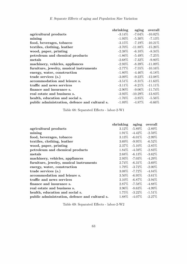
E Separate Effects of aging and Population Size Variation
shrinking aging overallagricultural products -3.14% -7.04% -10.02%mining -1.93% -5.30% -7.13%food, beverages, tobacco -3.15% -7.19% -10.21%textiles, clothing, leather -3.70% -11.88% -15.26%wood, paper, printing -2.38% -6.10% -8.34%petroleum and chemical products -1.86% -5.49% -7.25%metals -2.68% -7.32% -9.80%machinery, vehicles, appliances -2.93% -8.39% -11.09%furniture, jewelry, musical instruments -2.77% -7.55% -10.16%energy, water, construction -1.80% -4.46% -6.18%trade services (s.) -3.09% -9.22% -12.08%accommodation and leisure s. -3.51% -8.31% -11.63%traffic and news services -3.11% -8.21% -11.11%finance and insurance s. -2.90% -9.06% -11.74%real estate and business s. -3.93% -10.29% -13.83%health, education and social s. -1.76% -3.85% -5.56%public administration, defence and cultural s. -1.89% -4.87% -6.66%
Table 68: Separated Effects - labor-2-W1
shrinking aging overallagricultural products 3.12% -5.89% -2.89%mining 1.91% -4.42% -2.59%food, beverages, tobacco 3.13% -6.01% -2.99%textiles, clothing, leather 3.69% -9.95% -6.52%wood, paper, printing 2.37% -5.10% -2.85%petroleum and chemical products 1.84% -4.59% -2.83%metals 2.68% -6.13% -3.62%machinery, vehicles, appliances 2.93% -7.03% -4.29%furniture, jewelry, musical instruments 2.74% -6.31% -3.69%energy, water, construction 1.79% -3.72% -2.00%trade services (s.) 3.08% -7.72% -4.84%accommodation and leisure s. 3.50% -6.95% -3.61%traffic and news services 3.10% -6.87% -3.94%finance and insurance s. 2.87% -7.58% -4.88%real estate and business s. 3.96% -8.63% -4.99%health, education and social s. 1.75% -3.22% -1.51%public administration, defence and cultural s. 1.88% -4.07% -2.27%
Table 69: Separated Effects - labor-2-W2
63
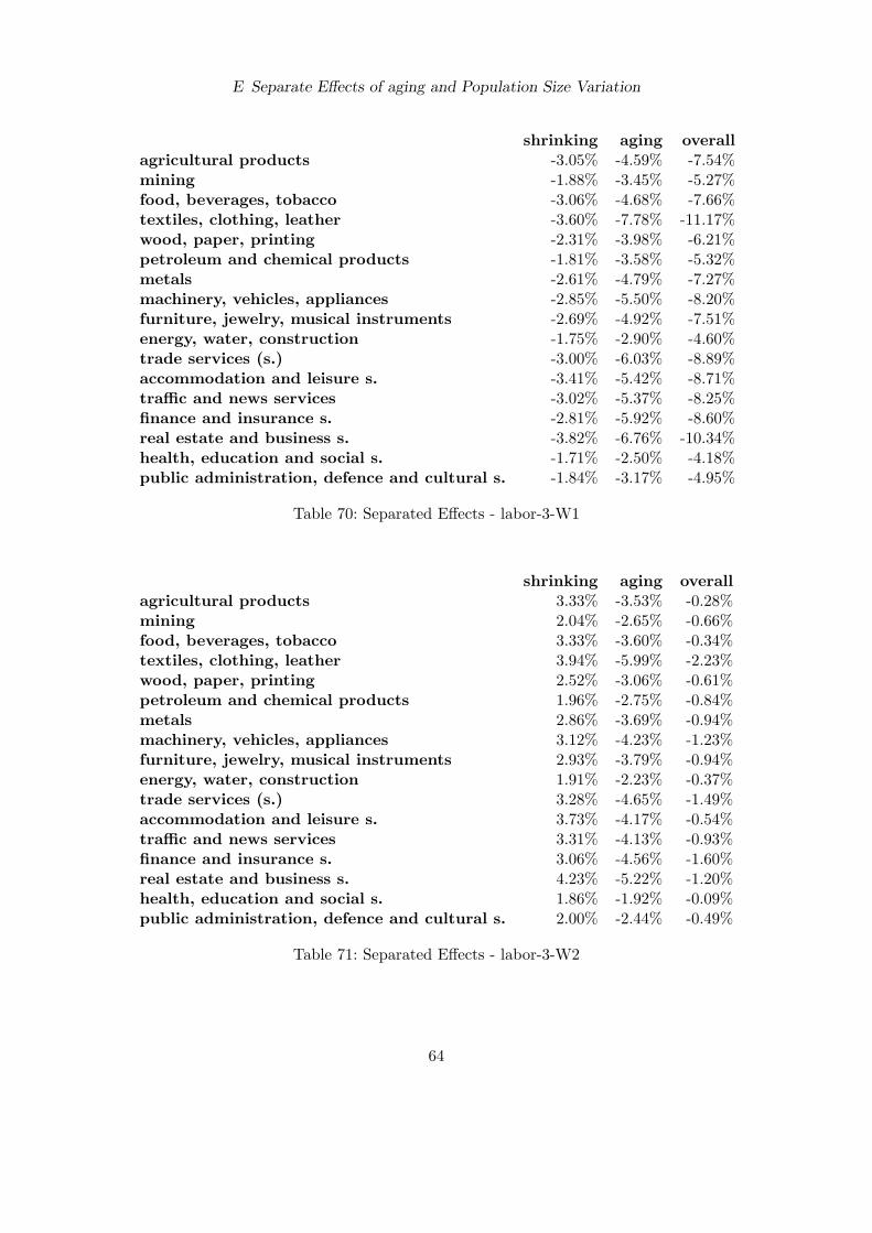
E Separate Effects of aging and Population Size Variation
shrinking aging overallagricultural products -3.05% -4.59% -7.54%mining -1.88% -3.45% -5.27%food, beverages, tobacco -3.06% -4.68% -7.66%textiles, clothing, leather -3.60% -7.78% -11.17%wood, paper, printing -2.31% -3.98% -6.21%petroleum and chemical products -1.81% -3.58% -5.32%metals -2.61% -4.79% -7.27%machinery, vehicles, appliances -2.85% -5.50% -8.20%furniture, jewelry, musical instruments -2.69% -4.92% -7.51%energy, water, construction -1.75% -2.90% -4.60%trade services (s.) -3.00% -6.03% -8.89%accommodation and leisure s. -3.41% -5.42% -8.71%traffic and news services -3.02% -5.37% -8.25%finance and insurance s. -2.81% -5.92% -8.60%real estate and business s. -3.82% -6.76% -10.34%health, education and social s. -1.71% -2.50% -4.18%public administration, defence and cultural s. -1.84% -3.17% -4.95%
Table 70: Separated Effects - labor-3-W1
shrinking aging overallagricultural products 3.33% -3.53% -0.28%mining 2.04% -2.65% -0.66%food, beverages, tobacco 3.33% -3.60% -0.34%textiles, clothing, leather 3.94% -5.99% -2.23%wood, paper, printing 2.52% -3.06% -0.61%petroleum and chemical products 1.96% -2.75% -0.84%metals 2.86% -3.69% -0.94%machinery, vehicles, appliances 3.12% -4.23% -1.23%furniture, jewelry, musical instruments 2.93% -3.79% -0.94%energy, water, construction 1.91% -2.23% -0.37%trade services (s.) 3.28% -4.65% -1.49%accommodation and leisure s. 3.73% -4.17% -0.54%traffic and news services 3.31% -4.13% -0.93%finance and insurance s. 3.06% -4.56% -1.60%real estate and business s. 4.23% -5.22% -1.20%health, education and social s. 1.86% -1.92% -0.09%public administration, defence and cultural s. 2.00% -2.44% -0.49%
Table 71: Separated Effects - labor-3-W2
64

E Separate Effects of aging and Population Size Variation
shrinking aging overallagricultural products 0.00% -5.73% -5.73%mining 0.00% -4.31% -4.31%food, beverages, tobacco 0.00% -5.85% -5.85%textiles, clothing, leather 0.00% -9.69% -9.69%wood, paper, printing 0.00% -4.96% -4.97%petroleum and chemical products 0.00% -4.47% -4.47%metals 0.00% -5.97% -5.97%machinery, vehicles, appliances 0.00% -6.84% -6.85%furniture, jewelry, musical instruments 0.00% -6.14% -6.15%energy, water, construction 0.00% -3.63% -3.63%trade services (s.) 0.00% -7.52% -7.52%accommodation and leisure s. 0.00% -6.76% -6.77%traffic and news services 0.00% -6.69% -6.69%finance and insurance s. 0.00% -7.38% -7.38%real estate and business s. -0.01% -8.41% -8.41%health, education and social s. 0.00% -3.13% -3.13%public administration, defence and cultural s. 0.00% -3.96% -3.96%
Table 72: Separated Effects - labor-4-W1
shrinking aging overallagricultural products 6.41% -4.64% 1.57%mining 3.92% -3.49% 0.30%food, beverages, tobacco 6.40% -4.73% 1.50%textiles, clothing, leather 7.58% -7.86% -0.71%wood, paper, printing 4.85% -4.02% 0.65%petroleum and chemical products 3.76% -3.62% 0.01%metals 5.51% -4.84% 0.40%machinery, vehicles, appliances 6.02% -5.55% 0.15%furniture, jewelry, musical instruments 5.62% -4.97% 0.44%energy, water, construction 3.66% -2.93% 0.62%trade services (s.) 6.31% -6.10% -0.10%accommodation and leisure s. 7.18% -5.48% 1.45%traffic and news services 6.37% -5.42% 0.67%finance and insurance s. 5.89% -5.98% -0.37%real estate and business s. 8.19% -6.83% 0.84%health, education and social s. 3.58% -2.53% 0.97%public administration, defence and cultural s. 3.84% -3.20% 0.51%
Table 73: Separated Effects - labor-4-W2
65

E Separate Effects of aging and Population Size Variation
shrinking aging overallagricultural products -7.81% -6.62% -14.06%mining -4.83% -4.98% -9.58%food, beverages, tobacco -7.86% -6.76% -14.30%textiles, clothing, leather -9.21% -11.17% -19.62%wood, paper, printing -5.93% -5.73% -11.34%petroleum and chemical products -4.65% -5.16% -9.58%metals -6.66% -6.88% -13.07%machinery, vehicles, appliances -7.28% -7.89% -14.62%furniture, jewelry, musical instruments -6.91% -7.09% -13.63%energy, water, construction -4.51% -4.19% -8.50%trade services (s.) -7.70% -8.67% -15.81%accommodation and leisure s. -8.74% -7.81% -16.09%traffic and news services -7.74% -7.72% -14.96%finance and insurance s. -7.23% -8.51% -15.24%real estate and business s. -9.69% -9.68% -18.47%health, education and social s. -4.41% -3.62% -7.89%public administration, defence and cultural s. -4.72% -4.57% -9.07%
Table 74: Separated Effects - labor-5-W1
shrinking aging overallagricultural products -1.70% -5.47% -7.10%mining -1.05% -4.11% -5.11%food, beverages, tobacco -1.71% -5.58% -7.23%textiles, clothing, leather -2.01% -9.25% -11.12%wood, paper, printing -1.29% -4.74% -5.97%petroleum and chemical products -1.01% -4.26% -5.23%metals -1.46% -5.70% -7.07%machinery, vehicles, appliances -1.59% -6.53% -8.02%furniture, jewelry, musical instruments -1.50% -5.86% -7.29%energy, water, construction -0.98% -3.46% -4.40%trade services (s.) -1.68% -7.17% -8.75%accommodation and leisure s. -1.90% -6.45% -8.28%traffic and news services -1.69% -6.38% -7.98%finance and insurance s. -1.57% -7.04% -8.52%real estate and business s. -2.14% -8.03% -10.00%health, education and social s. -0.96% -2.98% -3.92%public administration, defence and cultural s. -1.02% -3.77% -4.76%
Table 75: Separated Effects - labor-5-W2
66

E Separate Effects of aging and Population Size Variation
shrinking aging overallagricultural products -4.76% -7.77% -12.27%mining -2.94% -5.84% -8.62%food, beverages, tobacco -4.79% -7.94% -12.49%textiles, clothing, leather -5.62% -13.09% -18.16%wood, paper, printing -3.61% -6.73% -10.11%petroleum and chemical products -2.83% -6.06% -8.72%metals -4.07% -8.07% -11.80%machinery, vehicles, appliances -4.45% -9.25% -13.30%furniture, jewelry, musical instruments -4.20% -8.32% -12.26%energy, water, construction -2.74% -4.92% -7.52%trade services (s.) -4.69% -10.16% -14.46%accommodation and leisure s. -5.33% -9.16% -14.17%traffic and news services -4.72% -9.05% -13.42%finance and insurance s. -4.40% -9.98% -14.02%real estate and business s. -5.95% -11.32% -16.63%health, education and social s. -2.68% -4.26% -6.84%public administration, defence and cultural s. -2.87% -5.37% -8.08%
Table 76: Separated Effects - labor-6-W1
shrinking aging overallagricultural products 1.39% -6.59% -5.26%mining 0.85% -4.95% -4.14%food, beverages, tobacco 1.39% -6.72% -5.39%textiles, clothing, leather 1.64% -11.12% -9.61%wood, paper, printing 1.05% -5.71% -4.71%petroleum and chemical products 0.82% -5.14% -4.36%metals 1.19% -6.85% -5.74%machinery, vehicles, appliances 1.30% -7.86% -6.65%furniture, jewelry, musical instruments 1.22% -7.06% -5.90%energy, water, construction 0.80% -4.17% -3.41%trade services (s.) 1.37% -8.63% -7.36%accommodation and leisure s. 1.56% -7.77% -6.29%traffic and news services 1.38% -7.68% -6.39%finance and insurance s. 1.28% -8.47% -7.28%real estate and business s. 1.76% -9.64% -8.04%health, education and social s. 0.78% -3.60% -2.85%public administration, defence and cultural s. 0.84% -4.55% -3.75%
Table 77: Separated Effects - labor-6-W2
67

E Separate Effects of aging and Population Size Variation
shrinking aging overallagricultural products -3.11% -3.52% -6.53%mining -2.23% -2.51% -4.67%food, beverages, tobacco -2.73% -3.09% -5.74%textiles, clothing, leather -2.14% -2.42% -4.50%wood, paper, printing -2.70% -3.06% -5.68%petroleum and chemical products -2.42% -2.73% -5.07%metals -2.11% -2.39% -4.44%machinery, vehicles, appliances -1.92% -2.17% -4.03%furniture, jewelry, musical instruments -2.17% -2.45% -4.56%energy, water, construction -2.49% -2.82% -5.23%trade services (s.) -2.42% -2.74% -5.09%accommodation and leisure s. -2.46% -2.78% -5.17%traffic and news services -2.69% -3.04% -5.65%finance and insurance s. -2.49% -2.82% -5.23%real estate and business s. -4.23% -4.77% -8.80%health, education and social s. -1.98% -2.24% -4.17%public administration, defence and cultural s. -2.09% -2.36% -4.39%
Table 78: Separated Effects - prices-1-W1
shrinking aging overallagricultural products 0.02% -2.84% -2.82%mining 0.01% -2.03% -2.01%food, beverages, tobacco 0.02% -2.50% -2.48%textiles, clothing, leather 0.01% -1.95% -1.94%wood, paper, printing 0.02% -2.47% -2.45%petroleum and chemical products 0.01% -2.21% -2.19%metals 0.01% -1.93% -1.92%machinery, vehicles, appliances 0.01% -1.75% -1.74%furniture, jewelry, musical instruments 0.01% -1.98% -1.97%energy, water, construction 0.01% -2.28% -2.26%trade services (s.) 0.01% -2.21% -2.20%accommodation and leisure s. 0.01% -2.25% -2.23%traffic and news services 0.02% -2.46% -2.44%finance and insurance s. 0.01% -2.28% -2.26%real estate and business s. 0.03% -3.86% -3.84%health, education and social s. 0.01% -1.81% -1.80%public administration, defence and cultural s. 0.01% -1.91% -1.89%
Table 79: Separated Effects - prices-1-W2
68

E Separate Effects of aging and Population Size Variation
shrinking aging overallagricultural products -1.57% -4.21% -5.72%mining -1.12% -3.00% -4.09%food, beverages, tobacco -1.38% -3.70% -5.03%textiles, clothing, leather -1.08% -2.89% -3.94%wood, paper, printing -1.37% -3.66% -4.98%petroleum and chemical products -1.22% -3.27% -4.45%metals -1.07% -2.86% -3.89%machinery, vehicles, appliances -0.97% -2.60% -3.53%furniture, jewelry, musical instruments -1.10% -2.93% -3.99%energy, water, construction -1.26% -3.37% -4.58%trade services (s.) -1.22% -3.28% -4.46%accommodation and leisure s. -1.24% -3.33% -4.53%traffic and news services -1.36% -3.64% -4.95%finance and insurance s. -1.26% -3.37% -4.58%real estate and business s. -2.14% -5.70% -7.73%health, education and social s. -1.00% -2.68% -3.65%public administration, defence and cultural s. -1.05% -2.82% -3.85%
Table 80: Separated Effects - prices-2-W1
shrinking aging overallagricultural products 1.55% -3.51% -2.01%mining 1.11% -2.51% -1.43%food, beverages, tobacco 1.36% -3.09% -1.76%textiles, clothing, leather 1.06% -2.41% -1.38%wood, paper, printing 1.34% -3.05% -1.75%petroleum and chemical products 1.20% -2.73% -1.56%metals 1.05% -2.39% -1.36%machinery, vehicles, appliances 0.95% -2.17% -1.24%furniture, jewelry, musical instruments 1.08% -2.45% -1.40%energy, water, construction 1.24% -2.81% -1.61%trade services (s.) 1.20% -2.73% -1.56%accommodation and leisure s. 1.23% -2.78% -1.59%traffic and news services 1.34% -3.04% -1.74%finance and insurance s. 1.24% -2.81% -1.61%real estate and business s. 2.13% -4.77% -2.74%health, education and social s. 0.98% -2.24% -1.28%public administration, defence and cultural s. 1.04% -2.36% -1.35%
Table 81: Separated Effects - prices-2-W2
69

E Separate Effects of aging and Population Size Variation
shrinking aging overallagricultural products -1.53% -2.74% -4.23%mining -1.09% -1.95% -3.02%food, beverages, tobacco -1.34% -2.40% -3.71%textiles, clothing, leather -1.05% -1.88% -2.91%wood, paper, printing -1.33% -2.38% -3.67%petroleum and chemical products -1.19% -2.12% -3.28%metals -1.04% -1.86% -2.87%machinery, vehicles, appliances -0.94% -1.69% -2.61%furniture, jewelry, musical instruments -1.06% -1.91% -2.95%energy, water, construction -1.22% -2.19% -3.38%trade services (s.) -1.19% -2.13% -3.29%accommodation and leisure s. -1.21% -2.17% -3.35%traffic and news services -1.32% -2.36% -3.65%finance and insurance s. -1.22% -2.19% -3.38%real estate and business s. -2.08% -3.72% -5.73%health, education and social s. -0.97% -1.74% -2.69%public administration, defence and cultural s. -1.02% -1.83% -2.84%
Table 82: Separated Effects - prices-3-W1
shrinking aging overallagricultural products 1.65% -2.10% -0.48%mining 1.18% -1.50% -0.34%food, beverages, tobacco 1.45% -1.85% -0.42%textiles, clothing, leather 1.13% -1.44% -0.33%wood, paper, printing 1.43% -1.82% -0.42%petroleum and chemical products 1.28% -1.63% -0.37%metals 1.12% -1.43% -0.33%machinery, vehicles, appliances 1.01% -1.30% -0.30%furniture, jewelry, musical instruments 1.15% -1.46% -0.33%energy, water, construction 1.32% -1.68% -0.38%trade services (s.) 1.28% -1.64% -0.37%accommodation and leisure s. 1.31% -1.66% -0.38%traffic and news services 1.43% -1.82% -0.41%finance and insurance s. 1.32% -1.68% -0.38%real estate and business s. 2.27% -2.86% -0.65%health, education and social s. 1.05% -1.34% -0.30%public administration, defence and cultural s. 1.10% -1.41% -0.32%
Table 83: Separated Effects - prices-3-W2
70

E Separate Effects of aging and Population Size Variation
shrinking aging overallagricultural products 0.00% -3.42% -3.42%mining 0.00% -2.44% -2.44%food, beverages, tobacco 0.00% -3.00% -3.01%textiles, clothing, leather 0.00% -2.35% -2.35%wood, paper, printing 0.00% -2.97% -2.97%petroleum and chemical products 0.00% -2.65% -2.66%metals 0.00% -2.32% -2.32%machinery, vehicles, appliances 0.00% -2.11% -2.11%furniture, jewelry, musical instruments 0.00% -2.38% -2.38%energy, water, construction 0.00% -2.74% -2.74%trade services (s.) 0.00% -2.66% -2.66%accommodation and leisure s. 0.00% -2.71% -2.71%traffic and news services 0.00% -2.95% -2.96%finance and insurance s. 0.00% -2.74% -2.74%real estate and business s. 0.00% -4.64% -4.64%health, education and social s. 0.00% -2.18% -2.18%public administration, defence and cultural s. 0.00% -2.29% -2.29%
Table 84: Separated Effects - prices-4-W1
shrinking aging overallagricultural products 3.17% -2.76% 0.33%mining 2.26% -1.97% 0.24%food, beverages, tobacco 2.77% -2.43% 0.29%textiles, clothing, leather 2.17% -1.90% 0.23%wood, paper, printing 2.74% -2.40% 0.28%petroleum and chemical products 2.45% -2.15% 0.25%metals 2.14% -1.88% 0.22%machinery, vehicles, appliances 1.94% -1.70% 0.20%furniture, jewelry, musical instruments 2.20% -1.93% 0.23%energy, water, construction 2.53% -2.21% 0.26%trade services (s.) 2.46% -2.15% 0.25%accommodation and leisure s. 2.50% -2.19% 0.26%traffic and news services 2.73% -2.39% 0.28%finance and insurance s. 2.54% -2.21% 0.26%real estate and business s. 4.35% -3.76% 0.44%health, education and social s. 2.00% -1.76% 0.21%public administration, defence and cultural s. 2.11% -1.85% 0.22%
Table 85: Separated Effects - prices-4-W2
71

E Separate Effects of aging and Population Size Variation
shrinking aging overallagricultural products -3.95% -3.95% -7.76%mining -2.82% -2.82% -5.56%food, beverages, tobacco -3.47% -3.47% -6.83%textiles, clothing, leather -2.72% -2.72% -5.35%wood, paper, printing -3.43% -3.44% -6.75%petroleum and chemical products -3.06% -3.07% -6.03%metals -2.68% -2.69% -5.28%machinery, vehicles, appliances -2.43% -2.44% -4.80%furniture, jewelry, musical instruments -2.75% -2.76% -5.42%energy, water, construction -3.16% -3.17% -6.22%trade services (s.) -3.07% -3.08% -6.05%accommodation and leisure s. -3.12% -3.13% -6.15%traffic and news services -3.41% -3.42% -6.71%finance and insurance s. -3.16% -3.17% -6.21%real estate and business s. -5.35% -5.36% -10.43%health, education and social s. -2.51% -2.52% -4.96%public administration, defence and cultural s. -2.65% -2.65% -5.23%
Table 86: Separated Effects - prices-5-W1
shrinking aging overallagricultural products -0.85% -3.26% -4.09%mining -0.61% -2.33% -2.92%food, beverages, tobacco -0.75% -2.86% -3.59%textiles, clothing, leather -0.58% -2.24% -2.81%wood, paper, printing -0.74% -2.83% -3.55%petroleum and chemical products -0.66% -2.53% -3.17%metals -0.58% -2.21% -2.78%machinery, vehicles, appliances -0.52% -2.01% -2.52%furniture, jewelry, musical instruments -0.59% -2.27% -2.85%energy, water, construction -0.68% -2.61% -3.27%trade services (s.) -0.66% -2.54% -3.18%accommodation and leisure s. -0.67% -2.58% -3.23%traffic and news services -0.73% -2.82% -3.53%finance and insurance s. -0.68% -2.61% -3.27%real estate and business s. -1.16% -4.43% -5.54%health, education and social s. -0.54% -2.08% -2.60%public administration, defence and cultural s. -0.57% -2.19% -2.74%
Table 87: Separated Effects - prices-5-W2
72

E Separate Effects of aging and Population Size Variation
shrinking aging overallagricultural products -2.40% -4.65% -6.94%mining -1.71% -3.32% -4.97%food, beverages, tobacco -2.10% -4.08% -6.11%textiles, clothing, leather -1.65% -3.20% -4.78%wood, paper, printing -2.08% -4.04% -6.04%petroleum and chemical products -1.86% -3.61% -5.39%metals -1.62% -3.16% -4.72%machinery, vehicles, appliances -1.47% -2.87% -4.29%furniture, jewelry, musical instruments -1.67% -3.24% -4.85%energy, water, construction -1.92% -3.72% -5.56%trade services (s.) -1.86% -3.62% -5.41%accommodation and leisure s. -1.89% -3.68% -5.50%traffic and news services -2.07% -4.02% -6.00%finance and insurance s. -1.92% -3.72% -5.56%real estate and business s. -3.26% -6.29% -9.35%health, education and social s. -1.52% -2.96% -4.43%public administration, defence and cultural s. -1.60% -3.12% -4.67%
Table 88: Separated Effects - prices-6-W1
shrinking aging overallagricultural products 0.69% -3.93% -3.27%mining 0.49% -2.81% -2.33%food, beverages, tobacco 0.61% -3.46% -2.87%textiles, clothing, leather 0.48% -2.70% -2.24%wood, paper, printing 0.60% -3.42% -2.84%petroleum and chemical products 0.54% -3.05% -2.53%metals 0.47% -2.67% -2.22%machinery, vehicles, appliances 0.43% -2.43% -2.01%furniture, jewelry, musical instruments 0.48% -2.74% -2.28%energy, water, construction 0.55% -3.15% -2.62%trade services (s.) 0.54% -3.06% -2.54%accommodation and leisure s. 0.55% -3.11% -2.58%traffic and news services 0.60% -3.40% -2.82%finance and insurance s. 0.55% -3.15% -2.62%real estate and business s. 0.95% -5.33% -4.43%health, education and social s. 0.44% -2.51% -2.08%public administration, defence and cultural s. 0.46% -2.64% -2.19%
Table 89: Separated Effects - prices-6-W2
73