sectoral growth and energy consumption in south … growth and energy consumption in south and ......
TRANSCRIPT
Review of Economics & Finance
Submitted on 22/05/2017
Article ID: 1923-7529-2017-04-01-17
Anthony N. Rezitis, and Shaikh Mostak Ahammad
~ 1 ~
Sectoral Growth and Energy Consumption in South and Southeast
Asian Countries: Evidence from a Panel Data Approach
Prof. Dr. Anthony N. Rezitis (Correspondence author)
Department of Economics and Management
Faculty of Agriculture and Forestry, University of Helsinki,
P.O. Box 27, Latokartanonkaari 5, FI-00014, FINLAND
Tel: +358294158080 E-mail: [email protected]
Homepage: https://tuhat.helsinki.fi/portal/en/persons/anthony-rezitis(b636a186-169a-4831-920c-
5143635019cf).html
Dr. Shaikh Mostak Ahammad
Department of Accounting, Hajee Mohammad Danesh Science and Technology University,
Dinajpur 5200, BANGLADESH
Tel: +8801712083786 E-mail: [email protected]
Homepage: http://www.hstu.ac.bd/teacher/mostak
Abstract: This study examines the dynamic relationship between energy consumption and the
three major sectoral outputs (agricultural, manufacturing and service) in thirteen South and
Southeast Asian countries using a panel data framework for the period 1971–2012. It undertakes
panel cointegration analysis to investigate the long-run relationship between the variables. Also,
the panel vector error correction model (PVECM) and impulse response functions (IRFs) are
employed to examine the short- and long-run direction of causality and the effect of responses
between energy consumption and the three sectoral outputs. The empirical results reveal that the
long-run equilibrium relationship between energy consumption and the three sectoral outputs is
positive and statistically significant, indicating the existence of long-run co-movement among the
variables. The short- and long-run causality results support the existence of bidirectional causality
between energy consumption and the three sectoral outputs except for the short-run causality
between energy consumption and service sector output, which is unidirectional, running from
service sector output to energy consumption. The IRFs show that all variables reach the
equilibrium level within three to seven years from the initial shock.
Keywords: Panel cointegration; Panel vector error correction model; Panel causality; Panel impulse
response functions; SAARC; ASEAN
JEL Classifications: O47, O53, Q43
1. Introduction
The crucial role of energy consumption and its impact on economic growth have attracted the
interest of economists in recent years. The two energy crises in 1974 and 1981 have prompted
numerous empirical analyses regarding the relationships between energy consumption and
aggregate economic growth since the late 1970s (e.g. Kraft and Kraft, 1978; Erol and Yu, 1987;
Masih and Masih, 1997; Soytas and Sari, 2003; Huang et al., 2008; Lee and Chang, 2008; Ozturk et
ISSNs: 1923-7529; 1923-8401 © 2017 Academic Research Centre of Canada
~ 2 ~
al., 2010; Georgantopoulos, 2012). The related literature has been well documented by applying
both the panel data framework and time series analysis. However, in the literature, the evidence of
studies investigating the relationship between energy consumption and major economic sectoral
outputs (agricultural, manufacturing, service) is limited. Among the studies investigating the
relationships between energy consumption and sectoral outputs are those by Jumbe (2004), Chebbi
and Boujelbene (2008), Jamil and Ahmad (2010), Kwakwa (2012) and Nathan et al. (2013).
The present study explores the relationship between energy consumption and three major
sectoral outputs (agricultural, manufacturing and service) in thirteen South and Southeast Asian
countries by applying the panel data approach. The thirteen South and Southeast Asian countries
considered are Bangladesh, India, Nepal, Pakistan, Sri Lanka, Indonesia, Malaysia, the Philippines,
Thailand, Singapore, Brunei Darussalam, Myanmar and Vietnam. Of these thirteen countries, five
(Bangladesh, India, Nepal, Pakistan and Sri Lanka) are members of the South Asian Association for
Regional Cooperation (SAARC), while the remaining eight (Indonesia, Malaysia, the Philippines,
Thailand, Singapore, Brunei Darussalam, Myanmar and Vietnam) are members of the Association
of Southeast Asian Nations (ASEAN). These two organizations encompass about 6% of the Earth’s
total land area and about 32% of the world’s population, which are mostly shared by the
aforementioned countries.
The purpose of this study is to examine the extent to which energy consumption is related to
the agricultural, manufacturing and service sector outputs in thirteen South and Southeast Asian
countries. Following Mehrara (2007), the present study is based on an energy demand function and
employs a multivariate panel data framework with energy consumption (ENERGY), agricultural
sector output (AGR), manufacturing sector output (MAN) and service sector output (SER) to capture
the short- and long-run relationships between the series under consideration. In particular, the panel
cointegration analysis investigates the long-run relationship between the four series. The panel
vector error correction model (PVECM) captures the short- and long-run direction of the
relationships between energy consumption and the three sectoral outputs. It is worth mentioning
that some studies (Jumbe, 2004; Zamani, 2007; Chebbi and Boujelbene, 2008; Kouakou, 2011;
Liew et al., 2012; Nawaz et al., 2012; and Nwosa and Akinbobola, 2012) have investigated the
relationship between energy consumption and various sectoral outputs by using a bivariate model
between energy consumption and a particular economic sector, instead of a multivariate approach as
in the present study. However, in the case of bivariate analysis, there is the possibility of omitted
variable bias, as Lütkepohl (1982) indicated.
This study contributes to the literature in several ways. First, it might be the first study to use
the panel data approach to examine the growth dynamics and causality and provide IRFs between
energy consumption and agricultural sector, manufacturing sector and service sector outputs in
thirteen South and Southeast Asian countries. Among the previous studies, the study by Jamil and
Ahmad (2010) used individual time series techniques (i.e. cointegration and the vector error
correction model) to examine the relationship between electricity consumption and economic
growth on aggregated and disaggregated (residential, commercial, manufacturing and agricultural)
levels in Pakistan during the period 1960–2008. Second, the panel data approaches used in the
present study provide increased power information in comparison with the simple time series
methods, because the former derive information from both time and cross-sectional dimensions and
the latter derive information only from the time dimension. Finally, the approach of this study
extends the shrinkage estimator of the panel Vector Autoregressive (VAR) model developed by
Canova and Ciccarelli (2009) and Canova et al. (2007) to a panel vector error correction model
(PVECM). In particular, the framework of analysis of the panel VAR approach of Canova and

Review of Economics & Finance, Volume 10, Issue 4
~ 3 ~
Ciccarelli (2009) and Canova et al. (2007) is Bayesian in nature, with time variation, unit-specific
dynamics and cross-unit interdependencies. The PVECM of the present study does not assume full
homogeneity across individual supply chains, because different panel members are characterized by
different structure governing the relationship between energy consumption and output growth and
thus will very likely have different short-run price dynamics. Based on Doan (2012), the shrinkage
panel estimator provides more reliable estimates of the short-run dynamics that would be obtained
using simple individual-by-individual approaches.
The remainder of this study is presented as follows. The literature is discussed in section 2.
Section 3 presents a detailed outline of the methodology and data. Section 4 reports the empirical
results and discussion. Section 5 offers the conclusions of the study.
2. Literature Review
In the literature, the causal relationship between energy consumption and economic growth
could be categorized into four possible hypotheses: the growth, conservation, feedback and
neutrality hypotheses (Ozturk, 2010). First, the growth hypothesis refers to a condition whereby
energy consumption leads economic growth. It suggests that an increase in energy consumption
may contribute to economic growth, while a reduction in energy consumption may adversely affect
economic growth, indicating that the economy is energy dependent. Second, the conservation
hypothesis refers to a condition whereby economic growth leads energy consumption. It implies
that policies designed to reduce energy consumption will not adversely affect economic growth,
indicating that the economy is less energy dependent (Masih and Masih, 1997). The conservation
hypothesis is confirmed if an increase in economic growth causes an increase in energy
consumption. Third, the feedback hypothesis refers to a condition whereby causality runs in both
directions, that is, from energy consumption to economic growth and from economic growth to
energy consumption. It implies that energy consumption and economic growth are interconnected
and may very well serve as complements to each other. Finally, the neutrality hypothesis asserts a
condition whereby no causality exits in either direction between energy consumption and economic
growth. Similar to the conservation hypothesis, the neutrality hypothesis implies that energy
conservation policies may be pursued without adversely affecting the country’s economy. The
neutrality hypothesis is confirmed if an increase in economic growth does not cause an increase in
energy consumption and vice versa.
The previous studies relating to the relationship between energy consumption and economic
sectoral outputs (agricultural, manufacturing and service) pertaining to South and Southeast Asian
countries are inadequate. Among these studies, Jamil and Ahmad (2010), Zaman et al. (2011), Liew
et al. (2012), Qazi et al. (2012) and Ahmed and Zeshan (2014) employed a time series analysis to
investigate the relationship between energy consumption and economic sectoral outputs in Pakistan,
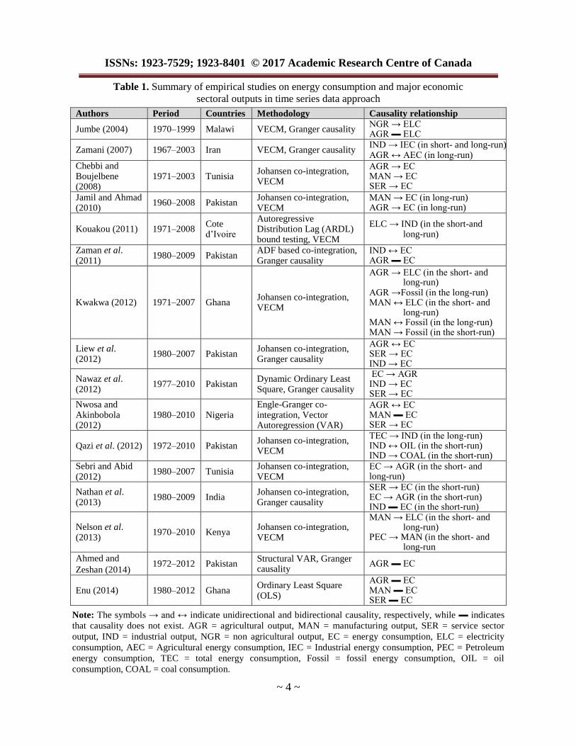
and Nathan et al. (2013) employed the same approach for India. Table 1 presents some of the most
recent research that studied energy consumption and various economic sectoral outputs using time
series analysis. In particular, the Johansen cointegration test proposed by Johansen and Juselius
(1990), the Engle–Granger co-integration test proposed by Engle and Granger (1987) and the
autoregressive distribution lag (ARDL) bound testing proposed by Pesaran et al. (2001) have been
used to estimate the cointegration between the variables under consideration. The Granger causality
test proposed by Granger (1969) and the vector error correction model (VECM) have been used to
test the direction of causality. The majority of the studies presented in Table 1 examined the
relationship between energy consumption and various economic sectoral outputs by conducting a
bivariate analysis.
ISSNs: 1923-7529; 1923-8401 © 2017 Academic Research Centre of Canada
~ 4 ~
Table 1. Summary of empirical studies on energy consumption and major economic
sectoral outputs in time series data approach
Authors Period Countries Methodology Causality relationship
Jumbe (2004) 1970–1999 Malawi VECM, Granger causality NGR → ELC AGR ▬ ELC
Zamani (2007) 1967–2003 Iran VECM, Granger causality IND → IEC (in short- and long-run) AGR ↔ AEC (in long-run)
Chebbi and Boujelbene (2008)
1971–2003 Tunisia Johansen co-integration, VECM
AGR → EC MAN → EC SER → EC
Jamil and Ahmad (2010)
1960–2008 Pakistan Johansen co-integration, VECM
MAN → EC (in long-run) AGR → EC (in long-run)
Kouakou (2011) 1971–2008 Cote d’Ivoire
Autoregressive Distribution Lag (ARDL) bound testing, VECM
ELC → IND (in the short-and long-run)
Zaman et al. (2011)
1980–2009 Pakistan ADF based co-integration, Granger causality
IND ↔ EC AGR ▬ EC
Kwakwa (2012) 1971–2007 Ghana Johansen co-integration, VECM
AGR → ELC (in the short- and long-run)
AGR →Fossil (in the long-run) MAN ↔ ELC (in the short- and
long-run) MAN ↔ Fossil (in the long-run) MAN → Fossil (in the short-run)
Liew et al. (2012)
1980–2007 Pakistan Johansen co-integration, Granger causality
AGR ↔ EC SER → EC IND → EC
Nawaz et al. (2012)
1977–2010 Pakistan Dynamic Ordinary Least Square, Granger causality
EC → AGR IND → EC SER → EC
Nwosa and Akinbobola (2012)
1980–2010 Nigeria Engle-Granger co-integration, Vector Autoregression (VAR)
AGR ↔ EC MAN ▬ EC SER → EC
Qazi et al. (2012) 1972–2010 Pakistan Johansen co-integration, VECM
TEC → IND (in the long-run) IND ↔ OIL (in the short-run) IND → COAL (in the short-run)
Sebri and Abid (2012)
1980–2007 Tunisia Johansen co-integration, VECM
EC → AGR (in the short- and long-run)
Nathan et al. (2013)
1980–2009 India Johansen co-integration, Granger causality
SER → EC (in the short-run) EC → AGR (in the short-run) IND ▬ EC (in the short-run)
Nelson et al. (2013)
1970–2010 Kenya Johansen co-integration, VECM
MAN → ELC (in the short- and long-run)
PEC → MAN (in the short- and long-run
Ahmed and
Zeshan (2014) 1972–2012 Pakistan
Structural VAR, Granger causality
AGR ▬ EC
Enu (2014) 1980–2012 Ghana Ordinary Least Square (OLS)
AGR ▬ EC MAN ▬ EC SER ▬ EC
Note: The symbols → and ↔ indicate unidirectional and bidirectional causality, respectively, while ▬ indicates
that causality does not exist. AGR = agricultural output, MAN = manufacturing output, SER = service sector
output, IND = industrial output, NGR = non agricultural output, EC = energy consumption, ELC = electricity
consumption, AEC = Agricultural energy consumption, IEC = Industrial energy consumption, PEC = Petroleum
energy consumption, TEC = total energy consumption, Fossil = fossil energy consumption, OIL = oil
consumption, COAL = coal consumption.
Review of Economics & Finance, Volume 10, Issue 4
~ 5 ~
Meanwhile, Qazi et al. (2012), Ahmed and Zeshan (2014) and Enu (2014) considered four
variate analyses to examine the relationship between energy consumption and sectoral outputs. In
particular, Qazi et al. (2012) considered industrial output, total employment, the consumer price
index (CPI) and aggregated and disaggregated energy consumption; Ahmed and Zeshan (2014)
focused on agricultural, industrial and service sector outputs and energy consumption; and Enu
(2014) investigated energy consumption, labor and capital formation to examine the relationship
between various sectoral outputs and energy consumption. In addition, Jamil and Ahmad (2010),
Kwakwa (2012), Sebri and Abid (2012) and Nelson et al. (2013) used trivariate analyses in their
studies. Specifically, Jamil and Ahmad (2010) considered electricity consumption, its price and the
GDP on aggregated and disaggregated levels; Kwakwa (2012) examined electricity consumption,
fossil energy consumption and the GDP on aggregated and disaggregated (agricultural and
manufacturing) levels; Sebri and Abid (2012) considered agricultural output, trade openness and
energy consumption on aggregated and disaggregated (oil and electricity) levels; and Nelson et al.
(2013) investigated manufacturing growth, electricity consumption and petroleum consumption.
Furthermore, Jumbe (2004), Zamani (2007), Chebbi and Boujelbene (2008), Kouakou (2011),
Zaman et al. (2011), Liew et al. (2012), Nawaz et al. (2012) and Nwosa and Akinbobola (2012)
considered a bivariate framework with energy or electricity consumption and particular sectoral
outputs to evaluate the relationship between energy consumption and various economic sectoral
outputs.
Considering the literature discussed above, the present study aims to investigate the
relationships between energy consumption and major economic sectoral outputs (agricultural,
manufacturing and service sector) in a panel data framework by incorporating a multivariate
analysis in thirteen South and Southeast Asian countries. Furthermore, unlike many of the previous
studies, the present study will discuss the causal relationship between energy consumption and the
three major economic sectoral outputs in relation to the four hypotheses categorized in the energy
consumption and economic growth literature.
3. Methodology
To facilitate a practical analysis of the relationship between sectoral growth and energy
consumption, this study uses several empirical methods, which include, first, panel unit root tests
(i.e. Harris and Tzavalis, 1999; Breitung, 2000; Levin et al., 2002; Im et al., 2003) to provide
information about the stationarity properties of the variables under consideration. Second, panel
cointegration tests (i.e. Pedroni, 1999) are performed to determine the presence of cointegration.
Third, the long-run cointegration parameters are estimated based on the studies by Pedroni (2001,
2004). Finally, a PVECM is used to test the short- and long-run panel causal relationship between
energy consumption and three major economic sectoral outputs (agricultural, manufacturing and
service) followed by panel IRFs. Note that the estimations are performed based on the procedures
developed in the work by Doan (2012) using the RATS 8.2 econometric software.
3.1 Panel unit root analysis
The determination of the stationarity properties of the variables under consideration is an
important step in an empirical analysis, since applying the usual ordinary least square estimator in
non-stationary variables results in spurious regressions. To determine the order of integration of the
variables, the present study utilizes four different panel unit root tests. The first is the Levin, Lin
and Chu (LLC) test developed by Levin et al. (2002), the second is the Harris and Tzavalis (HT)
ISSNs: 1923-7529; 1923-8401 © 2017 Academic Research Centre of Canada
~ 6 ~
test developed by Harris and Tzavalis (1999), the third is the Im, Pesaran and Shin (IPS) test
developed by Im et al. (2003) and the fourth is the Breitung test developed by Breitung (2000).
3.2 Panel cointegration analysis
To test the existence of the long-run equilibrium relationship among the variables under
consideration (i.e. lnENERGY, lnAGR, lnMAN and lnSER), a panel cointegration test proposed by
Pedroni (1999) is used. Pedroni (1999, 2004) developed two sets of tests for cointegration, which
include seven statistics. In the first set, four out of the seven are based on pooling along the within-
dimension, which is known as panel cointegration statistics: they are the panel v-statistic, panel ρ-
statistic, panel PP-statistic and panel ADF-statistic. With regard to the second set, the remaining
three are based on pooling along the between-dimension, which is known as group mean panel
cointegration statistics: they are the group ρ-statistic, group PP-statistic and group ADF-statistic.
The long-run relationship between energy consumption and the three sectoral outputs (e.g.
agricultural sector, manufacturing sector and service sector) is given by Equation (1):
1 2 3ln ln ln ln
1,..., ; 1971 to 2012 (1)
it i i t i t i t itENERGY AGR MAN SER
for i N t
where αi is a fixed-effect parameter while β1i, β2i and β3i are the slope parameters. εit are the
estimated residuals, which represent deviations from the long-run relationship. ENERGYit refers to
the energy consumption, AGR is the real gross domestic product of the agricultural sector, MAN is
the real gross domestic product of the manufacturing sector and SER is the real gross domestic
product of the service sector.
Based on a number of studies written by Pedroni (2000, 2001, 2004, 2007), the current study
employs two estimators to estimate the long-run parameters of the cointegration relationships,
which is given by Equation (1). The first estimator is the fully modified ordinary least squares
(FMOLS), which was originally developed by Phillips and Hansen (1990) and extended by Hansen
(1992). The second estimator is the dynamic ordinary least squares (DOLS), which was proposed by
Stock and Watson (1993). It is worth mentioning that the least squares estimated parameters in
Equation (1) suffer from simultaneity bias due to the correlation between the left-hand side variable
(lnENERGYit) and the error term (εit) and from dynamic endogeneity due to serial correlation of the
error term (εit). The FMOLS estimator used in estimating Equation (1) corrects the estimates and
covariance matrix for endogeneity, while the DOLS estimator eliminates the endogeneity by
including the current lags and leads of the first difference of the right-hand variables (lnAGR,
lnMAN and lnSER) in the regression of Equation (1).1
3.3 Panel short-run and long-run causality analysis
Since the cointegration analysis can only determine the relationship among the variables, not
the direction of causality, it is usual practice to examine the causal direction among the variables
once cointegration is established. The current study employs a two-step procedure to test the
causality. The first step is to estimate the long-run model (FMOLS) specified in Equation (1) to
calculate the residuals. The second step is to define the one-lagged residuals as the error correction
term (ECT), which will be included in the panel vector error correction model. In particular, the
variables are considered as in the first difference plus the error correction term (ECT) as an
exogenous variable. The dynamic PVECM can be formulated as follows:
1 Time trend is not included in Equation (1) because it was not found to be statistically significant.
Review of Economics & Finance, Volume 10, Issue 4
~ 7 ~
1 11 , 12 , 13 ,
1 1 1
14 , 1 1 1
1
2 21 , 22 , 23
1 1 1
ln ln ln ln
ln (2.1)
ln ln ln ln
p p p
it i li i t l li i t l li i t l
l l l
p
li i t l i it it
l
p p p
it i li i t l li i t l li
l l l
ENERGY ENERGY AGR MAN
SER u
AGR ENERGY AGR MA
,
24 , 2 1 2
1
3 31 , 32 , 33 ,
1 1 1
34 , 3 1 3
1
4 41
1
ln (2.2)
ln ln ln ln
ln (2.3)
ln ln
i t l
p
li i t l i it it
l
p p p
it i li i t l li i t l li i t l
l l l
p
li i t l i it it
l
p
it i li
l
N
SER u
MAN ENERGY AGR MAN
SER u
SER ENERG
, 42 , 43 ,
1 1
44 , 4 1 4
1
ln ln
ln (2.4)
1,...,13; 1971 to 2012
p p
i t l li i t l li i t l
l l
p
li i t l i it it
l
Y AGR MAN
SER u
for i t
where Δ is the first-difference operator; p is the lag length set at two based on the satisfaction of the
classical assumptions on the error term;2 εit is the residuals from the panel FMOLS estimation of
Equation (1); and uit is the serially uncorrelated error term. In the energy consumption (ENERGY)
Eq. (2.1), the short-run causality from agricultural sector output, manufacturing sector output and
service sector output to energy consumption is examined, based on0 12: 0li liH ,
0 13: 0li liH and0 14: 0li liH , respectively. In the agricultural sector output (AGR) Eq.
(2.2), the short-run causality from energy consumption, manufacturing sector output and service
sector output to agricultural sector output is examined, based on0 21: 0li liH ,
0 23: 0li liH
and0 24: 0li liH , respectively. In the manufacturing sector output (MAN) Eq. (2.3), the short-
run causality from energy consumption, agricultural sector output and service sector output to
manufacturing sector output is examined, based on0 31: 0li liH ,
0 32: 0li liH and
0 34: 0li liH , respectively. Finally, in the service sector output (SER) Eq. (2.4), short-run
causality from energy consumption, agricultural sector output and manufacturing sector output to
service sector output is examined, based on0 41: 0li liH ,
0 42: 0li liH and0 43: 0li liH ,
respectively. The long-run causality in each Eq. (2.1)–(2.4) is examined by investigating the
statistical significance of the t-statistic for the coefficient on the respective error correction term
(εit).3
2 Lee and Chang (2008) showed the procedure to identify the optimal lag. For the selection of the
optimal lag, the test process is started by lag one (P = 1) and it continues until the error terms are free of serial correlation. In this study, lag two (P = 2) satisfies the classical assumptions on the error term.
3 Time trends are not included in Equations (2.1)-(2.4) because they were not found to be statistically significant.
ISSNs: 1923-7529; 1923-8401 © 2017 Academic Research Centre of Canada
~ 8 ~
3.4 Data
The data used in this study consist of annual observations from 1971 to 2012. The energy
consumption data were obtained from the World Bank Development Indicators and the remaining
three sectors’ (agricultural, manufacturing and service) data were obtained from the United Nations’
National Accounts Main Aggregates Database for thirteen South and Southeast Asian countries,
namely Bangladesh, India, Nepal, Pakistan, Sri Lanka, Indonesia, Malaysia, the Philippines,
Thailand, Singapore, Brunei Darussalam, Myanmar and Vietnam. The remaining countries were
omitted due to the unavailability of data for all the variables (i.e. data from 1971 to 2012). The
multivariate panel data approach includes the natural logarithm of energy use (lnENERGY) in
kilowatt per oil equivalent, real gross domestic product of the agricultural sector (lnAGR) in
constant 2005 U.S. dollars, real gross domestic product of the manufacturing sector (lnMAN) in
constant 2005 U.S. dollars and real gross domestic product of the service sector (lnSER) in constant
2005 U.S. dollars.
4. Results and Discussion
4.1 Panel unit root results
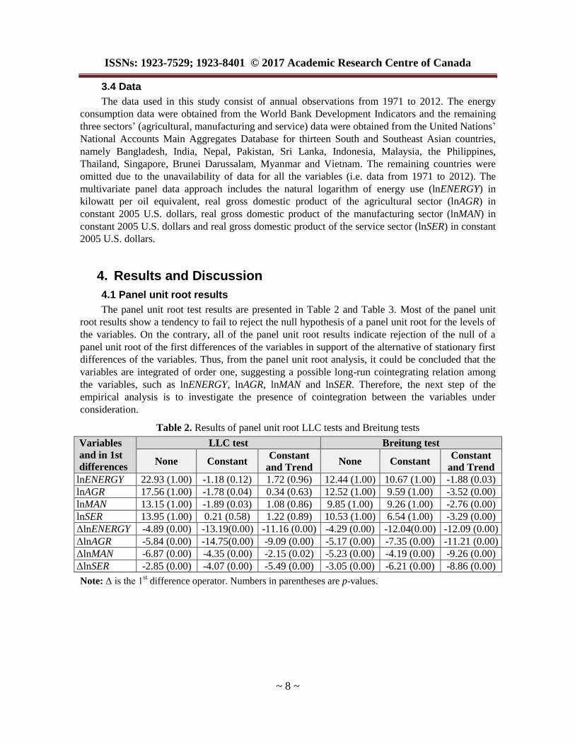
The panel unit root test results are presented in Table 2 and Table 3. Most of the panel unit
root results show a tendency to fail to reject the null hypothesis of a panel unit root for the levels of
the variables. On the contrary, all of the panel unit root results indicate rejection of the null of a
panel unit root of the first differences of the variables in support of the alternative of stationary first
differences of the variables. Thus, from the panel unit root analysis, it could be concluded that the
variables are integrated of order one, suggesting a possible long-run cointegrating relation among
the variables, such as lnENERGY, lnAGR, lnMAN and lnSER. Therefore, the next step of the
empirical analysis is to investigate the presence of cointegration between the variables under
consideration.
Table 2. Results of panel unit root LLC tests and Breitung tests
Variables
and in 1st
differences
LLC test Breitung test
None Constant Constant
and Trend None Constant
Constant
and Trend
lnENERGY 22.93 (1.00) -1.18 (0.12) 1.72 (0.96) 12.44 (1.00) 10.67 (1.00) -1.88 (0.03)
lnAGR 17.56 (1.00) -1.78 (0.04) 0.34 (0.63) 12.52 (1.00) 9.59 (1.00) -3.52 (0.00)
lnMAN 13.15 (1.00) -1.89 (0.03) 1.08 (0.86) 9.85 (1.00) 9.26 (1.00) -2.76 (0.00)
lnSER 13.95 (1.00) 0.21 (0.58) 1.22 (0.89) 10.53 (1.00) 6.54 (1.00) -3.29 (0.00)
ΔlnENERGY -4.89 (0.00) -13.19(0.00) -11.16 (0.00) -4.29 (0.00) -12.04(0.00) -12.09 (0.00)
ΔlnAGR -5.84 (0.00) -14.75(0.00) -9.09 (0.00) -5.17 (0.00) -7.35 (0.00) -11.21 (0.00)
ΔlnMAN -6.87 (0.00) -4.35 (0.00) -2.15 (0.02) -5.23 (0.00) -4.19 (0.00) -9.26 (0.00)
ΔlnSER -2.85 (0.00) -4.07 (0.00) -5.49 (0.00) -3.05 (0.00) -6.21 (0.00) -8.86 (0.00)
Note: Δ is the 1st difference operator. Numbers in parentheses are p-values.
Review of Economics & Finance, Volume 10, Issue 4
~ 9 ~
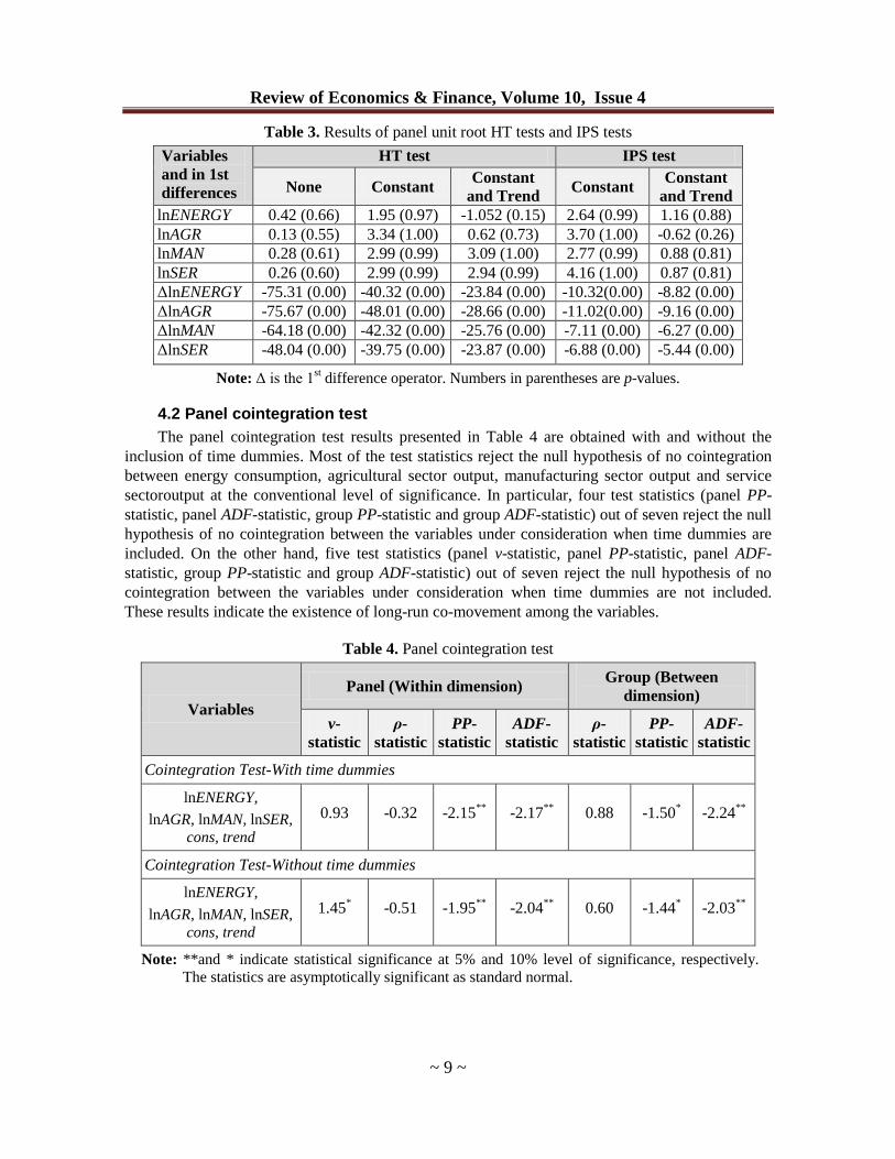
Table 3. Results of panel unit root HT tests and IPS tests
Variables
and in 1st
differences
HT test IPS test
None Constant Constant
and Trend Constant
Constant
and Trend
lnENERGY 0.42 (0.66) 1.95 (0.97) -1.052 (0.15) 2.64 (0.99) 1.16 (0.88)
lnAGR 0.13 (0.55) 3.34 (1.00) 0.62 (0.73) 3.70 (1.00) -0.62 (0.26)
lnMAN 0.28 (0.61) 2.99 (0.99) 3.09 (1.00) 2.77 (0.99) 0.88 (0.81)
lnSER 0.26 (0.60) 2.99 (0.99) 2.94 (0.99) 4.16 (1.00) 0.87 (0.81)
ΔlnENERGY -75.31 (0.00) -40.32 (0.00) -23.84 (0.00) -10.32(0.00) -8.82 (0.00)
ΔlnAGR -75.67 (0.00) -48.01 (0.00) -28.66 (0.00) -11.02(0.00) -9.16 (0.00)
ΔlnMAN -64.18 (0.00) -42.32 (0.00) -25.76 (0.00) -7.11 (0.00) -6.27 (0.00)
ΔlnSER -48.04 (0.00) -39.75 (0.00) -23.87 (0.00) -6.88 (0.00) -5.44 (0.00)
Note: Δ is the 1st difference operator. Numbers in parentheses are p-values.
4.2 Panel cointegration test
The panel cointegration test results presented in Table 4 are obtained with and without the
inclusion of time dummies. Most of the test statistics reject the null hypothesis of no cointegration
between energy consumption, agricultural sector output, manufacturing sector output and service
sectoroutput at the conventional level of significance. In particular, four test statistics (panel PP-
statistic, panel ADF-statistic, group PP-statistic and group ADF-statistic) out of seven reject the null
hypothesis of no cointegration between the variables under consideration when time dummies are
included. On the other hand, five test statistics (panel v-statistic, panel PP-statistic, panel ADF-
statistic, group PP-statistic and group ADF-statistic) out of seven reject the null hypothesis of no
cointegration between the variables under consideration when time dummies are not included.
These results indicate the existence of long-run co-movement among the variables.
Table 4. Panel cointegration test
Variables
Panel (Within dimension) Group (Between
dimension)
v-
statistic
ρ-
statistic
PP-
statistic
ADF-
statistic
ρ-
statistic
PP-
statistic
ADF-
statistic
Cointegration Test-With time dummies
lnENERGY,
lnAGR, lnMAN, lnSER,
cons, trend
0.93 -0.32 -2.15**
-2.17**
0.88 -1.50* -2.24
**
Cointegration Test-Without time dummies
lnENERGY,
lnAGR, lnMAN, lnSER,
cons, trend
1.45* -0.51 -1.95
** -2.04
** 0.60 -1.44
* -2.03
**
Note: **and * indicate statistical significance at 5% and 10% level of significance, respectively.
The statistics are asymptotically significant as standard normal.
ISSNs: 1923-7529; 1923-8401 © 2017 Academic Research Centre of Canada
~ 10 ~
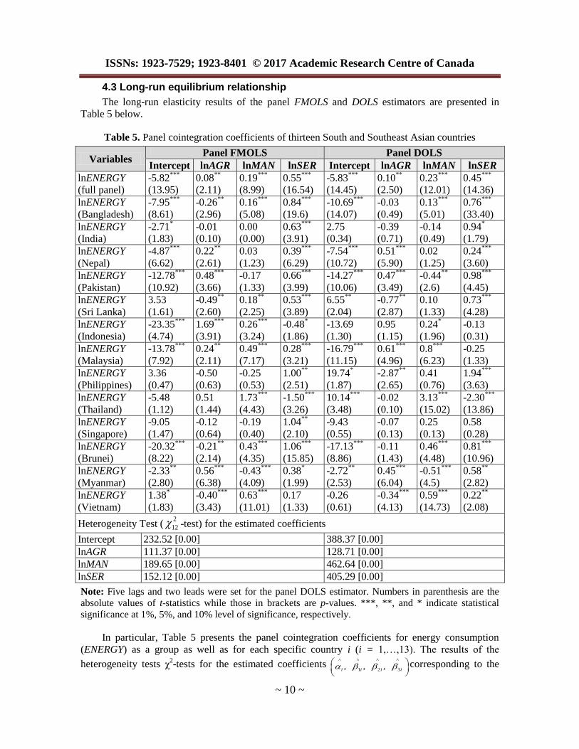
4.3 Long-run equilibrium relationship
The long-run elasticity results of the panel FMOLS and DOLS estimators are presented in
Table 5 below.
Table 5. Panel cointegration coefficients of thirteen South and Southeast Asian countries
Variables Panel FMOLS Panel DOLS
Intercept lnAGR lnMAN lnSER Intercept lnAGR lnMAN lnSER
lnENERGY
(full panel)
-5.82***
(13.95)
0.08**
(2.11)
0.19***
(8.99)
0.55***
(16.54)
-5.83***
(14.45)
0.10**
(2.50)
0.23***
(12.01)
0.45***
(14.36)
lnENERGY
(Bangladesh)
-7.95***
(8.61)
-0.26**
(2.96)
0.16***
(5.08)
0.84***
(19.6)
-10.69***
(14.07)
-0.03
(0.49)
0.13***
(5.01)
0.76***
(33.40)
lnENERGY
(India)
-2.71*
(1.83)
-0.01
(0.10)
0.00
(0.00)
0.63***
(3.91)
2.75
(0.34)
-0.39
(0.71)
-0.14
(0.49)
0.94*
(1.79)
lnENERGY
(Nepal)
-4.87***
(6.62)
0.22**
(2.61)
0.03
(1.23)
0.39***
(6.29)
-7.54***
(10.72)
0.51***
(5.90)
0.02
(1.25)
0.24***
(3.60)
lnENERGY
(Pakistan)
-12.78***
(10.92)
0.48***
(3.66)
-0.17
(1.33)
0.66***
(3.99)
-14.27***
(10.06)
0.47***
(3.49)
-0.44**
(2.6)
0.98***
(4.45)
lnENERGY
(Sri Lanka)
3.53
(1.61)
-0.49**
(2.60)
0.18**
(2.25)
0.53***
(3.89)
6.55**
(2.04)
-0.77**
(2.87)
0.10
(1.33)
0.73***
(4.28)
lnENERGY
(Indonesia)
-23.35***
(4.74)
1.69***
(3.91)
0.26***
(3.24)
-0.48*
(1.86)
-13.69
(1.30)
0.95
(1.15)
0.24*
(1.96)
-0.13
(0.31)
lnENERGY
(Malaysia)
-13.78***
(7.92)
0.24**
(2.11)
0.49***
(7.17)
0.28***
(3.21)
-16.79***
(11.15)
0.61***
(4.96)
0.8***
(6.23)
-0.25
(1.33)
lnENERGY
(Philippines)
3.36
(0.47)
-0.50
(0.63)
-0.25
(0.53)
1.00**
(2.51)
19.74*
(1.87)
-2.87**
(2.65)
0.41
(0.76)
1.94***
(3.63)
lnENERGY
(Thailand)
-5.48
(1.12)
0.51
(1.44)
1.73***
(4.43)
-1.50***
(3.26)
10.14***
(3.48)
-0.02
(0.10)
3.13***
(15.02)
-2.30***
(13.86)
lnENERGY
(Singapore)
-9.05
(1.47)
-0.12
(0.64)
-0.19
(0.40)
1.04**
(2.10)
-9.43
(0.55)
-0.07
(0.13)
0.25
(0.13)
0.58
(0.28)
lnENERGY
(Brunei)
-20.32***
(8.22)
-0.21**
(2.14)
0.43***
(4.35)
1.06***
(15.85)
-17.13***
(8.86)
-0.11
(1.43)
0.46***
(4.48)
0.81***
(10.96)
lnENERGY
(Myanmar)
-2.33**
(2.80)
0.56***
(6.38)
-0.43***
(4.09)
0.38*
(1.99)
-2.72**
(2.53)
0.45***
(6.04)
-0.51***
(4.5)
0.58**
(2.82)
lnENERGY
(Vietnam)
1.38*
(1.83)
-0.40***
(3.43)
0.63***
(11.01)
0.17
(1.33)
-0.26
(0.61)
-0.34***
(4.13)
0.59***
(14.73)
0.22**
(2.08)
Heterogeneity Test (2
12 -test) for the estimated coefficients
Intercept 232.52 [0.00] 388.37 [0.00]
lnAGR 111.37 [0.00] 128.71 [0.00]
lnMAN 189.65 [0.00] 462.64 [0.00]
lnSER 152.12 [0.00] 405.29 [0.00]
Note: Five lags and two leads were set for the panel DOLS estimator. Numbers in parenthesis are the
absolute values of t-statistics while those in brackets are p-values. ***, **, and * indicate statistical
significance at 1%, 5%, and 10% level of significance, respectively.
In particular, Table 5 presents the panel cointegration coefficients for energy consumption
(ENERGY) as a group as well as for each specific country i (i = 1,…,13). The results of the
heterogeneity tests χ2-tests for the estimated coefficients
^ ^ ^ ^
1 2 3, , ,i i i i
corresponding to the

Review of Economics & Finance, Volume 10, Issue 4
~ 11 ~
variables under consideration (intercepti, lnAGRi, lnMANi, lnSERi) are also reported in Table 5. The
null hypothesis of the heterogeneity test is that each individual coefficient is equal to the average of
the group.
A primary inspection of the empirical results reported in Table 5 indicates that the FMOLS and
DOLS estimators produce very similar results in terms of the sign, magnitude and statistical
significance of the parameter estimates for the full panel and slightly different results for the
individual countries.
The third row of Table 5 presents the estimated parameters of the cointegration vector
corresponding to the full panel, that is, the whole group of 13 South and Southeast Asian countries.
All the coefficients of the full panel are positive and statistically significant at the 5% level of
significance. The estimates of the full-panel FMOLS indicate that a 1% increase in agricultural
sector output increases energy consumption by 0.08%; a 1% increase in manufacturing sector
output increases energy consumption by 0.19%; and a 1% increase in service sector output
increases energy consumption by 0.55%. The estimates of the full-panel DOLS indicate that a 1%
increase in agricultural sector output increases energy consumption by 0.10%; a 1% increase in
manufacturing sector output increases energy consumption by 0.23%; and a 1% increase in service
sector output increases energy consumption by 0.45%. Note that energy consumption shows a
higher response to service sector output followed by manufacturing sector output and agricultural
sector output for both FMOLS and DOLS models. The FMOLS and DOLS estimates of individual
countries indicate that the effect of agricultural sector output on energy consumption is positive and
statistically significant in about 5 out of 13 countries in the FMOLS model and 4 out of 13 countries
in the DOLS model, while it is negative and statistically significant in about 4 out of 13 countries in
the FMOLS model and 3 out of 13 countries in the DOLS model. The negative and significant
responses of energy consumption to the agricultural sector output of these countries might be a
reason why farmers in the particular countries do not use energy as a modernized tool to enhance
agricultural productivity efficiently and effectively. With regard to the manufacturing sector output
and service sector output, most of the effects on energy consumption are positive. The heterogeneity
tests for the estimated coefficients presented in the last five rows of Table 5 reject the hypothesis of
equality of the individual estimated coefficient to the corresponding average panel (group)
coefficient presented in the third row of the table.
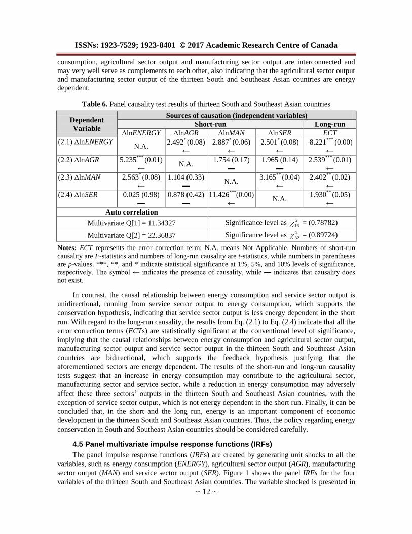
4.4 Short-run and long-run causality analysis
Table 6 presents the results of the short- and long-run causality tests for the panel data set
under consideration. Based on Table 6, the short-run dynamics in Eq. (2.1) indicate that agricultural
sector output (AGR), manufacturing sector output (MAN) and service sector output (SER) have an
impact on energy consumption (ENERGY),since their F-statistics are statistically significant at the
10% level of significance. The results of Eq. (2.2) provide evidence that energy consumption
(ENERGY) has predictive power to forecast agricultural sector output (AGR). On the other hand,
manufacturing sector output (MAN) and service sector output (SER) do not have any predictive
power to forecast agricultural sector output since their F-statistics are statistically insignificant. In
terms of Eq. (2.3), it appears that energy consumption and service sector output have a causal effect
on manufacturing sector output, while agricultural sector output does not have any causal effect on
manufacturing sector output. The results of Eq. (2.4) show that manufacturing sector output has an
impact on service sector output. However, energy consumption and agricultural sector output do not
have any impact on service sector output. Therefore, it is implied that the short-run causality
relationships between energy consumption and agricultural sector output and between energy
consumption and manufacturing sector output in thirteen South and Southeast Asian countries are
bidirectional, which supports the feedback hypothesis. These relationships indicate that energy
ISSNs: 1923-7529; 1923-8401 © 2017 Academic Research Centre of Canada
~ 12 ~
consumption, agricultural sector output and manufacturing sector output are interconnected and
may very well serve as complements to each other, also indicating that the agricultural sector output
and manufacturing sector output of the thirteen South and Southeast Asian countries are energy
dependent.
Table 6. Panel causality test results of thirteen South and Southeast Asian countries
Dependent
Variable
Sources of causation (independent variables)
Short-run Long-run
ΔlnENERGY ΔlnAGR ΔlnMAN ΔlnSER ECT
(2.1) ΔlnENERGY
N.A.
2.492* (0.08)
←
2.887* (0.06)
←
2.501* (0.08)
←
-8.221***
(0.00)
←
(2.2) ΔlnAGR
5.235***
(0.01)
← N.A.
1.754 (0.17)
▬
1.965 (0.14)
▬
2.539***
(0.01)
←
(2.3) ΔlnMAN
2.563* (0.08)
←
1.104 (0.33)
▬ N.A.
3.165**
(0.04)
←
2.402**
(0.02)
←
(2.4) ΔlnSER
0.025 (0.98)
▬
0.878 (0.42)
▬
11.426***
(0.00)
← N.A.
1.930**
(0.05)
←
Auto correlation
Multivariate Q[1] = 11.34327 Significance level as 2
16 = (0.78782)
Multivariate Q[2] = 22.36837 Significance level as 2
32 = (0.89724)
Notes: ECT represents the error correction term; N.A. means Not Applicable. Numbers of short-run
causality are F-statistics and numbers of long-run causality are t-statistics, while numbers in parentheses
are p-values. ***, **, and * indicate statistical significance at 1%, 5%, and 10% levels of significance,
respectively. The symbol ← indicates the presence of causality, while ▬ indicates that causality does
not exist.
In contrast, the causal relationship between energy consumption and service sector output is
unidirectional, running from service sector output to energy consumption, which supports the
conservation hypothesis, indicating that service sector output is less energy dependent in the short
run. With regard to the long-run causality, the results from Eq. (2.1) to Eq. (2.4) indicate that all the
error correction terms (ECTs) are statistically significant at the conventional level of significance,
implying that the causal relationships between energy consumption and agricultural sector output,
manufacturing sector output and service sector output in the thirteen South and Southeast Asian
countries are bidirectional, which supports the feedback hypothesis justifying that the
aforementioned sectors are energy dependent. The results of the short-run and long-run causality
tests suggest that an increase in energy consumption may contribute to the agricultural sector,
manufacturing sector and service sector, while a reduction in energy consumption may adversely
affect these three sectors’ outputs in the thirteen South and Southeast Asian countries, with the
exception of service sector output, which is not energy dependent in the short run. Finally, it can be
concluded that, in the short and the long run, energy is an important component of economic
development in the thirteen South and Southeast Asian countries. Thus, the policy regarding energy
conservation in South and Southeast Asian countries should be considered carefully.
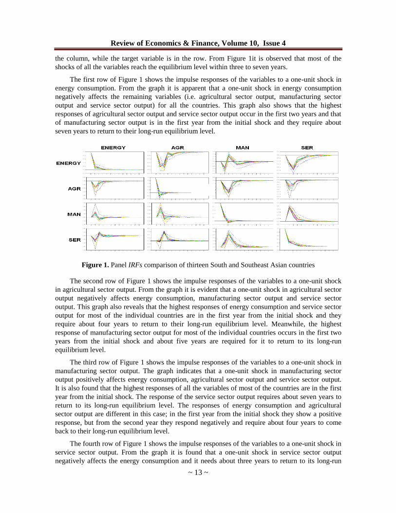
4.5 Panel multivariate impulse response functions (IRFs)
The panel impulse response functions (IRFs) are created by generating unit shocks to all the
variables, such as energy consumption (ENERGY), agricultural sector output (AGR), manufacturing
sector output (MAN) and service sector output (SER). Figure 1 shows the panel IRFs for the four
variables of the thirteen South and Southeast Asian countries. The variable shocked is presented in
Review of Economics & Finance, Volume 10, Issue 4
~ 13 ~
the column, while the target variable is in the row. From Figure 1it is observed that most of the
shocks of all the variables reach the equilibrium level within three to seven years.
The first row of Figure 1 shows the impulse responses of the variables to a one-unit shock in
energy consumption. From the graph it is apparent that a one-unit shock in energy consumption
negatively affects the remaining variables (i.e. agricultural sector output, manufacturing sector
output and service sector output) for all the countries. This graph also shows that the highest
responses of agricultural sector output and service sector output occur in the first two years and that
of manufacturing sector output is in the first year from the initial shock and they require about
seven years to return to their long-run equilibrium level.
Figure 1. Panel IRFs comparison of thirteen South and Southeast Asian countries
The second row of Figure 1 shows the impulse responses of the variables to a one-unit shock
in agricultural sector output. From the graph it is evident that a one-unit shock in agricultural sector
output negatively affects energy consumption, manufacturing sector output and service sector
output. This graph also reveals that the highest responses of energy consumption and service sector
output for most of the individual countries are in the first year from the initial shock and they
require about four years to return to their long-run equilibrium level. Meanwhile, the highest
response of manufacturing sector output for most of the individual countries occurs in the first two
years from the initial shock and about five years are required for it to return to its long-run
equilibrium level.
The third row of Figure 1 shows the impulse responses of the variables to a one-unit shock in
manufacturing sector output. The graph indicates that a one-unit shock in manufacturing sector
output positively affects energy consumption, agricultural sector output and service sector output.
It is also found that the highest responses of all the variables of most of the countries are in the first
year from the initial shock. The response of the service sector output requires about seven years to
return to its long-run equilibrium level. The responses of energy consumption and agricultural
sector output are different in this case; in the first year from the initial shock they show a positive
response, but from the second year they respond negatively and require about four years to come
back to their long-run equilibrium level.
The fourth row of Figure 1 shows the impulse responses of the variables to a one-unit shock in
service sector output. From the graph it is found that a one-unit shock in service sector output
negatively affects the energy consumption and it needs about three years to return to its long-run

ISSNs: 1923-7529; 1923-8401 © 2017 Academic Research Centre of Canada
~ 14 ~
equilibrium level. Furthermore, it positively affects agricultural sector output and manufacturing
sector output, which are the highest in the first two years from the initial shock and require about
five years to come back to their long-run equilibrium level.
5. Conclusions and Policy Implications
This study examines the relationship between energy consumption and the three major sectoral
outputs (agricultural, manufacturing and service) in thirteen South and Southeast Asian countries
using the panel data approach. It uses panel cointegration analysis to estimate the dynamic
relationships, the PVECM to detect the direction of short-run and long-run causality and panel IRFs
to examine the effect of shocks between energy consumption and the three sectoral outputs under
consideration.
The panel cointegration analysis reveals that the long-run equilibrium relationship between
energy consumption, agricultural sector, manufacturing sector and service sector are positive and
statistically significant, indicating the existence of long-run co-movement among the variables. The
panel short-run causality results evidence bidirectional causality between energy consumption and
agricultural sector and between energy consumption and manufacturing sector, supporting the
feedback hypothesis, while the causal relationship between energy consumption and service sector
is unidirectional, running from service sector to energy consumption, which supports the
conservation hypothesis. These results indicate that the agricultural sector and manufacturing sector
of the thirteen South and Southeast Asian countries are energy dependent, but the service sector is
less energy dependent. The panel long-run causality results provide evidence that the causal
relationship between energy consumption and the three sectoral outputs (agricultural,
manufacturing and service) are bidirectional, which supports the feedback hypothesis, indicating
that energy consumption and agricultural sector, manufacturing sector and service sector are
interconnected and may very well serve as complements to each other, which also suggests that in
the long run, the agricultural sector, manufacturing sector and service sector of the thirteen South
and Southeast Asian countries are energy dependent. The results of the short-run and long-run
causality tests suggest that an increase in energy consumption may contribute to the agricultural
sector, manufacturing sector and service sector outputs, while a reduction in energy consumption
may adversely affect these three sectors’ output in the thirteen South and Southeast Asian countries,
with the exception of service sector, which is not energy dependent in the short run. The panel
multivariate impulse response functions indicate that: (i) the responses to shocks of all the variables
reach the equilibrium level within three to seven years in the time period, (ii) a one-unit shock in
energy consumption negatively affects agricultural sector, manufacturing sector and service sector,
(iii) a one-unit shock in agricultural sector negatively affects energy consumption, manufacturing
sector and service sector, (iv) a one-unit shock in manufacturing sector positively affects energy
consumption, agricultural sector and service sector and (v) a one-unit shock in service sector
negatively affects energy consumption but positively affects agricultural sector and manufacturing
sector.
Finally, the empirical results of the present study might give policymakers a better
understanding of the relationship between energy consumption and the three economic sectoral
outputs (agricultural, manufacturing and service) to formulate energy policies in the thirteen South
and Southeast Asian countries. The dynamic relationships between energy consumption and
economic sectoral outputs in the present study clearly indicate that energy consumption has a
significant impact on the three economic sectoral outputs. This means that continuous energy
consumption may contribute to a continuous increase in agricultural sector, manufacturing sector
Review of Economics & Finance, Volume 10, Issue 4
~ 15 ~
and service sector outputs and a continuous reduction in energy consumption may compromise the
development of agricultural sector, manufacturing sector and service sector outputs, indicating that
sectoral outputs are fundamentally motivated by energy consumption. However, the excessive
consumption of energy may create long-run environmental consequences. As a result, to avoid
negative shocks to the economic development in the thirteen South and Southeast Asian countries,
the policymakers should formulate well-planned short-term and long-term energy conservation
policies taking into consideration the sector-specific links with energy consumption and the possible
long-run environmental impacts.
Acknowledgements: The co-author (Shaikh Mostak Ahammad) is grateful to the state
scholarship foundation (IKY), Greece for the financial support for his PhD studies
at the University of Patras (Greece).
References
[1] Ahmed, V., Zeshan, M. (2014). “Decomposing change in energy consumption of the
agricultural sector in Pakistan”. Agrarian South: Journal of Political Economy, 3(3): 1-34.
http://ags.sagepub.com/content/3/3/369.full.pdf+html.
[2] Breitung, J. (2001). “The local power of some unit root tests for panel data”, In: Badi H.
Baltagi, Thomas B. Fomby, R. Carter Hill (eds.) Nonstationary Panels, Panel Cointegration,
and Dynamic Panels (Advances in Econometrics, Volume 15) Emerald Group Publishing
Limited, 161-177.
[3] Canova, F. and Ciccarelli, M. (2009). “Estimating multicounty VAR models”, International
Economics Review, 50(3): 929-959.
[4] Canova, F., Ciccarelli, M. and Ortega, E. (2007). “Similarities and convergence in G-7 cycles”,
Journal of Monetary Economics, 54(3): 850-878.
[5] Chebbi, H.E., Boujelbene, Y. (2008). “Agriculture and Non-Agriculture Outputs and Energy
Consumption in Tunisia: Empirical Evidences from Cointegration and Causality”. 12th
Congress of the European Association of Agriculture Economist – EAAE 2008.
[6] Doan, T.A. (2012). “RATS handbook for panel and grouped data”. Draft Version, Estima.
[7] Engle, R.F., Granger, C.W.J. (1987). “Co-integration and error correction: representation,
estimation and testing”, Econometrica, 55(2): 251-276.
[8] Enu, P. (2014). “Sectoral estimation of the impact of electricity consumption on real output in
Ghana”, International Journal of Economics, Commerce and Management, 2(9): 1-18.
[9] Erol, U., Yu, E.S.H. (1987). “Time series analysis of the causal relationships between U.S.
energy and employment”, Resources and Energy, 9(1): 75-89.
[10] Georgantopoulos, A. (2012). “Electricity consumption and economic growth: Analysis and
forecasts using VAR/VEC approach for Greece with capital formation”, International Journal
of Energy Economics and Policy, 2(4): 263-278.
[11] Granger, C.W.J. (1969). “Investigating causal relations by econometric models and cross
spectral methods”, Econometrica, 37(3): 424-438.
[12] Hansen, B. (1992). “Efficient estimation and testing of cointegrating vectors in the presence of
deterministic trends”, Journal of Econometrics, 53(1): 87-121.
[13] Harris, R. D. F., Tzavalis, E. (1999). “Inference for unit roots in dynamic panels where the
time dimensions is fixed”, Journal of Econometrics, 91(2): 201-226.

ISSNs: 1923-7529; 1923-8401 © 2017 Academic Research Centre of Canada
~ 16 ~
[14] Huang, B.N., Hwang, M.J., Yang, C.W. (2008). “Causal relationship between energy
consumption and GDP growth revisited: a dynamic panel data approach”, Ecological
Economics, 67(1): 41-54.
[15] Im, K., Pesaran, M.H., Shin, Y. (2003). “Testing for unit roots in heterogeneous panels”,
Journal of Econometrics, 115(1): 53-74.
[16] Jamil, F., Ahmad, A. (2010). “The Relationship between Electricity Consumption, Electricity
Price and GDP in Pakistan”, Energy Policy, 38(10): 6016- 6025.
[17] Johansen, S., Juselius, K. (1990). “Maximum likelihood estimation and inference on
cointegration with applications to the demand for money”, Oxford Bulletin of Economics and
Statistics, 52(2): 169-210.
[18] Jumbe, C. (2004). “Cointegration and causality between electricity consumption and GDP:
empirical evidence from Malawi”, Energy Economics, 26(1): 61-68.
[19] Kouakou, A.K. (2011). “Economic growth and electricity consumption in Cote d’Ivoire:
evidence from time series analysis”, Energy Policy, 39(6): 3638-3644.
[20] Kraft, J., Kraft, A. (1978). “On the relationship between energy and GNP”, Journal of Energy
and Development, 3(2): 401-403.
[21] Kwakwa, P.A. (2012). “Disaggregated energy consumption and economic growth in Ghana”,
International Journal of Energy Economics and Policy, 2(1): 34-40.
[22] Lee, C.C., Chang, C.P. (2008). “Energy consumption and economic growth in Asian
economies: a more comprehensive analysis using panel data”, Resource and Energy
Economics, 30(1): 50-65.
[23] Levin, A., Lin, C.-F., Chu, S.-S. (2002). “Unit root tests in panel data: Asymptotic and finite-
sample properties”, Journal of Econometrics, 108(1): 1-24.
[24] Liew, V.K., Nathan, T.M., Wong, W. (2012). “Are sectoral outputs in Pakistan led by energy
consumption? ”, Economic Bulletin, 32(3): 2326-2331.
[25] Lütkepohl, H. (1982). “Non-causality due to omitted variables”, Journal of Econometrics,
19(2-3): 267-378.
[26] Masih, A.M.M., Masih, R. (1997). “On the Temporal causal relationship between energy
consumption, real income, and prices: some evidence from Asian-energy dependent NICs
based on a multivariate cointegration/vector error-correction approach”, Journal of Policy
Modeling, 19 (4): 417-440.
[27] Mehrara, M. (2007). “Energy consumption and economic growth: the case of oil exporting
countries”, Energy Policy, 35(5): 2939-2945.
[28] Nathan, T.M., Liew, V.K., “Al-Mamun, A. (2013). “Effect of primary energy consumption
towards disagregated sectoral outputs of India”, Asian Journal of Research in Business
Economics and Management, 3(11): 260-268.
[29] Nawaz, M., Sadaqat, M., Awan, N.W., Qureshi, M. (2012). “Energy consumption and
economic growth: A disaggregate approach”, Asian Economic and Financial Review, 2(1):
255-261.
[30] Nelson, O., Mukras, M.S., Siringi, E.M. (2013). “Causality between disaggregated energy
consumption and manufacturing growth in Kenya: An empirical approach”, Journal of
Economics and Sustainable Development, 4(16): 29-36.
[31] Nwosa, P. I., Akinbobola, T.O. (2012). “Aggregate energy consumption and sectoral output in
Nigeria”, African Research Review, 6(4): 206-215.
[32] Ozturk, I. (2010). “A literature survey on energy–growth nexus”, Energy Policy, 38(8): 340-
349.
Review of Economics & Finance, Volume 10, Issue 4
~ 17 ~
[33] Ozturk, I., Aslan, A., Kalyoncu, H. (2010). “Energy consumption and economic growth
relationship: Evidence from panel data for low and middle income countries”, Energy Policy,
38(8): 4422-4428.
[34] Pedroni, P. (1999). “Critical values for cointegration tests in heterogeneous panels with
multiple regressors”, Oxford Bulletin of Economics and Statistics, 61(S), 653-670.
[35] Pedroni, P. (2000). “Fully Modified OLS for Heterogenous Cointegrated Panels”, In: Baltagi
B. (ed.), Nonstationary Panels, Panel Cointegration, and Dynamic Panels, Advances in
Econometrics, Vol. 15, Amsterdam: JAI Press, pp. 93-130.
[36] Pedroni, P. (2001). “Purchasing power parity tests in cointegrated panels”, Review of
Economics and Statistics, 83(4): 727-731.
[37] Pedroni, P. (2004). “Panel cointegration: asymptotic and finite sample properties of pooled
time series tests with an application to the PPP hypothesis”, Econometric Theory, 20(3): 597-
625.
[38] Pedroni, P. (2007). “Social capital, barriers to production and capital shares: implications for
the importance of parameter heterogeneity from a nonstationary panel approach”, Journal of
Applied Econometrics, 22(2): 429-451.
[39] Pesaran, M., Shin, Y., Smith, R.J. (2001). “Bounds testing approaches to the analysis of level
relationships”, Journal of Applied Econometrics, 16(3): 289-326.
[40] Phillips, P., Hansen, B. (1990). “Statistical Inference in Instrumental Variables Regression
with I(1) Processes”, Review of Economic Studies, 57(1): 99-125.
[41] Phillips, P.C.B., Perron, P. (1988). “Testing for a unit root in time series regression”,
Biometrica, 75(2): 335-346.
[42] Qazi, A.Q., Ahmed, K., Mudassar, M. (2012). “Disaggregate energy consumption and
industrial output in Pakistan: An empirical analysis”, Discussion Paper 2012-29, June 25,
2012. http://www.economics-ejournal.org/economics/discussionpapers/2012-29.
[43] Sebri, M., Abid, M. (2012). “Energy use for economic growth: A trivariate analysis from
Tunisian agriculture sector”, Energy Policy, 48(C): 711-716.
[44] Soytas, U., Sari, R. (2003). “Energy consumption and GDP: causality relationship in G-7
countries and emerging markets”, Energy Economics, 25(1): 33-37.
[45] Stock, J., Watson, M. (1993). “A simple estimator of cointegrating vector in higher order
integrating systems”, Econometrica, 61(4): 783-820.
[46] Zaman, K., Khan, M.M., Saloom, Z. (2011). “Bivariate cointegration between energy
consumption and development factors: A case study of Pakistan”, International Journal of
Green Energy, 8(8): 820-833.
[47] Zamani, M. (2007). “Energy consumption and economic activities in Iran”, Energy Economics,
29(6): 1135-1140.