Agent Sentiment and Stock Market Predictability

Chandler Lutz∗

July 15, 2010

Abstract

Using only market return data we create an original index via a dynamic factor model

for stock market sentiment. We find that rising sentiment relates to rising returns. Using

our index we develop one-step ahead out-of-sample forecasts for market weighted returns.

These forecasts outperform a random walk plus drift model and improve on previous

out-of-sample exercises. We also employ dynamic Bayesian Model Averaging (BMA) and

develop Two-Stage Bayesian Model Averaging (2SBMA). We find that these techniques

can improve forecast performance. Lastly, we use our index to quantitatively chronicle

sentiment cycles. We find that sentiment cycles often lead bear markets.

Keywords: Behavioral Finance, Agent Sentiment, Financial Forecasting

∗University of California, Riverside, Department of Economics, Email: chandler.lutz@email.ucr.edu

1

“I can calculate the motions of the heavenly bodies, but not the madness of people.”

-Sir Isaac Newton

Accounts of agent sentiment in asset markets have persisted throughout history: beginning

with the Dutch tulip mania in the 1600s through the recent credit crisis of 2008. Developing

further insights into how sentiment affects stocks is paramount to our understanding of financial

markets.

Classical finance theory posits that investors are fully rational. In this framework, arbi-

trageurs make a risk-free profit on any security mispricing. This leads to the ideas of the

efficient market hypothesis and elusive stock market predictability. The notion of predicting

asset returns out-of-sample has intrigued researchers and practitioners for centuries. How-

ever, investors outperforming market averages or stock booms and busts have no place in the

traditional finance literature. The large failure of the economic and financial literature in fore-

casting the stock market has added credence to the classical theories. Yet the outstanding

performance of investors such as Warren Buffett and George Soros and the many bubbles and

crashes throughout history created a dichotomy between researchers the practitioners. Be-

havioral finance attempts to close this chasm by making two basic assumptions: (1) Market

participants are subject to sentiment or beliefs that are not necessarily supported by the facts

and (2) there are limits and risks to arbitrage.1 Using behavioral models, researchers attempt

to explain booms and busts and stock market anomalies that escape traditional economic and

financial research.

This paper attempts to extend the behavioral literature. Using a dynamic factor model and

Bayesian estimation we develop a novel index for agent sentiment in the stock market. We argue

that our index closely matches previous documentations of stock market bubbles. Using our

index we conduct various in-sample regressions and find a relationship between rising sentiment

and rising returns. This supports the idea of sentiment driven bubbles. We use our index to

forecast out-of-sample market-weighted returns. We find that conditioning on sentiment allows

1Abreu and Brunnermeier (2003) produce a bubble model without this second assumption. Battalio andSchultz (2006) find no evidence of short-sale constraints during the 1990s tech bubble.

2

us to develop models that outperform the benchmark random walk plus drift under a rolling

window and recursive estimation. While conducting our forecasting exercise we also develop

an extension of the dynamic Bayesian model averaging (BMA) procedure of Raftery et al.

(2005). We call this new technique two-stage Bayesian model averaging (2SBMA). The more

flexible 2SBMA approach allows researchers to average forecasts from different models each

with a different number of specifications. The technique of Raftery et al. (2005) requires that

each forecasting model must have the same number of specifications. We find that both the

BMA and 2SBMA procedures exhibit superior out-of-sample performance compared to the

benchmark model. Lastly, we modify the Bry-Boschan (1971) algorithm to quantitatively date

sentiment cycles. We find that sentiment cycles often lead general stock market cycles.

From a theoretical standpoint, De Long et al. (1990a,b) and Lee, Shleifer and Thaler (1991)

implicate noise traders into their models. They find that sentiment affects a broad cross-

section of stocks. Abreu and Brunnermeier (2003) construct a bubble model. They contend

that sentiment and a dispersion of opinions affect market returns. When a bubble develops

arbitrageurs may be limited by the costs or risks for short selling. One could could imagine

that these limitations are not constant across firms. D’Avolio (2002) finds that young, small,

unprofitable and growth stocks are more costly to buy and sell short. Baker and Wurgler (2006,

2007) find that these types of companies are most affected by sentiment. These firms do not

pay dividends, have shorter earnings histories and are more volatile. These characteristics make

companies more speculative in nature. This allows investors to plausibly defend a wider range

of valuations. All these findings lead to the “Hard-to-Value, Difficult-to-Arbitrage” (HV-DA)

hypothesis. This theory posits that the same stocks that are hard to value are also difficult to

arbitrage. Baker and Wurgler (2006) develop a sentiment index at the macro level and run in-

sample regressions on a cross-section of stock returns. They conclude that the HV-DA stocks

are most affected by sentiment. Brown and Cliff (2004,2005) use sentiment driven surveys

to study the predictability of asset returns. Lemmon and Portniaguina (2006) and Qui and

Welch (2004) use consumer confidence to investigate return predictability. Glushkov (2006)

augments Baker and Wurgler’s (2006) sentiment index by including sentiment surveys, mutual

3

fund flows, and short-sale and margin data. Using this new index, Glushkov (2006) develops a

sentiment beta. This beta measures how much an individual stock is affected by sentiment.2

Glushkov (2006) also accounts for size and volatility. He finds that stocks with more analyst

following, greater institutional ownership and a higher likelihood of S&P500 membership are

more affected by sentiment. Chung and Yeh (2009) account for regime changes with a Markov

process. They use Baker and Wurgler’s sentiment index to study the cross-section of stock

returns. They find that sentiment’s predictive power only prevails under a ‘bullish’ regime.

The index of Baker and Wurgler (2006, 2007) is the closest in spirit to the index developed

in this paper. They consider six components for their index: The closed-end fund discount,

the number and average first day return on IPOs, NYSE share turnover, the equity share of

new issues and the dividend premium.3 They compile their index by using the first principle

component as the weight for each series. Baker and Wurgler (2006) develop an annual index for

sentiment. This index captures swings in sentiment through the sample. Baker and Wurgler

(2007) extend the index to monthly data. We plot Baker and Wurgler’s (2007) monthly index

(BWsent) against bear markets in figure 3. The sample period is from 1965M07 to 2007M12.

BWsent generally follows the overall trends in sentiment. For example, Baker and Wurgler’s

index captures the low-sentiment times in the mid-1970s. Yet BWsent produces counterin-

tuitive results for other bear episodes. Baker and Wurgler’s index peaks in 2001M02. This

is nearly a year after the tech crash and the bear market in 2000M03. This is particularly

surprising since the tech boom and bust is largely attributed to agent sentiment (see, for ex-

ample, Shiller, 2006). Additionally, BWsent climbs through the bear market that began in

1968M11 and reaches it global maximum in 1969M12. Baker and Wurgler’s index also remains

high through the bear market of the early 1980s. These features of BWsent contradict our

expectations. Sentiment should peak prior to the end of speculative episodes and crash as bear

markets take hold.

[Insert figure 3 here]

2This is synonymous to the popular market beta which relates a stock’s return and the market average.3Data and further explanations are available from Jeffrey Wurgler’s website http://pages.stern.nyu.

edu/~jwurgler/

4

Using their index, Baker and Wurgler (2006, 2007) also contend that high sentiment trans-

lates into lower future returns for the HV-DA stocks. Baker, Wugler and Yuan (2009) find sim-

ilar results for other industrialized nations. These results contradict the theoretical findings of

Abreu and Brunnermeier (2003). Abreu and Brunnermeier conclude that rational arbitrageurs

have a profit incentive to ride sentiment bubbles over some interval. In other words, over a cer-

tain interval rising sentiment relates to rising returns. Furthermore, Lutz (2010d) considers the

smoothed earnings-price ratio (ep10) as a measure of agent sentiment.4 He considers in-sample

regressions and an out of sample forecasting exercise. Lutz (2010d) finds that rising sentiment

(as measured by ep10) relates to rising returns for stocks without dividends and companies

without earnings. These results contradict the findings in Baker and Wurgler (2006, 2007).

Furthermore, Lutz (2010d) contends that Baker and Wurgler’s sentiment index ‘mis-times’ the

conclusion of certain sentiment episodes.

In addition, Baker and Wurgler’s index is difficult to calculate in real time. Their index is

subject to data revisions. For example, one of their index components is the equity share of

new issues. This series is only available monthly. Also, this series is subject to data revisions

and only available for past values.

We use only market data to develop our sentiment index. This produces two main advan-

tages: (1) There are no data revisions or measurement errors in our index components and

(2) practitioners, firms or policymakers could easily calculate our index in real-time and make

decisions based on current information. We use a dynamic factor model to calculate our index.

We find that our index more closely corresponds to sentiment bubbles and crashes than the

index proposed by Baker and Wurgler (2006, 2007).5 Our index also closely coincides with

anecdotal evidence of sentiment.

Another area of interest in the behavioral literature is stock market predictability. The

empirical literature discovered an underreaction of stock prices to earnings announcements or

4ep10 is average earnings over the last ten years divided by the price for the S&P500. Averaging earningsover a ten year period mitigates business cycle effects. The result, according to Shiller (2006), is a series thatcaptures agent sentiment in the stock market.

5See figures 2 and 3

5

other news. Researchers have also found an overreaction to a series of good or bad news.

Barberis, Shleifer and Vishny (1998) construct a behavioral model to account for these anoma-

lies. In a theoretical model Barberis, Huang and Santos (2001) find predictability in returns

in aggregate. There appears to be consensus in the behavioral literature that asset returns are

in fact predictable but the degree of this predictability is an open debate. Most of the work

is concerned with in-sample predictability. There has been little success in out-of sample fore-

casting exercises especially when considering market-weighted returns. Timmermann (2008)

documents the failure of previous works in forecasting returns out-of-sample and highlights

the difficulty of such endeavors in his paper, “Elusive return predictability.” Furthermore,

Timmermann (2008) uses various models where the regressors are either past return values

or standard macro of finance variables. He concludes that stock returns may contain local

predictability (for short time periods). Then a wide range of practitioners will learn the model

and it loses its power. Timmermann (2008) contends that this makes forecasting returns over

long periods of time an extremely difficult task. It should be noted that Timmermann (2008)

does not consider any behavioral variables. Campbell and Thompson (2007) find out-of-sample

predictability for some variables compared the benchmark random-walk plus drift. However,

they restrict the signs of their regression coefficients. In our forecasting exercise we use a vari-

ety of models and condition on our sentiment index to construct out-of-sample forecasts. We

consider both rolling window and recursive estimation periods. We find that some of these

models outperform the benchmark random-walk plus drift over an extended sample period. In

particular, we find that linear models and forecast combinations outperform the benchmark.6

Our forecasting results suggest that sentiment affects a broad cross-section of returns but they

do not specify which stocks are most affected by sentiment.

I The Data

Baker and Wurgler (2006, 2007), among others, find that agent sentiment affects small, young,

and volatile firms, firms without earnings or dividends, and firms in distress. These results

6See tables VI through XI for our forecasting results

6

help motivate the choice of the series used to construct the sentiment index in this paper.

We use long-short portfolios of equal weighted returns based on dividends, size and earnings.

More specifically, we examine the difference between market returns for stocks that do not pay

dividends and those that do, companies with earnings less than or equal to zero and those

with positive earnings and small and large firms. We define a small (large) firm as one whose

market cap is in the bottom (upper) 20 percent. We also consider the equal weighted returns

of low momentum firms. We classify firms whose returns are in the bottom ten percent for the

previous two to twelve months as having low momentum. We use the returns on low momentum

firms to represent companies in distress. The series are all monthly and compiled from Kenneth

French’s data library.7 The correlation matrix for these variables is presented in table I. The

data for the series comprised from momentum, size, and dividends are available from 1927M07,

but the data for earnings begins in 1951M07. Hence, our data contains 698 observations ranging

from 1951M07 to 2009M08. We use the returns from the S&P500 to incorporate the findings

of Glushkov (2006). He found that after controlling for size and volatility that larger stocks

with a higher likelihood of S&P500 membership are more affected by sentiment.8

[Insert table I here]

Since we derive the data from market returns our index has two main advantages over other

sentiment measures and macroeconomic indicators. First, there is no measurement error and

no need for the data to be revised. This eliminates the uncertainty related to surveying and

sampling that plagues many macro variables. Second, firms and policymakers could compile

the data in real time and extend our model to make decisions based on current information.9

We abbreviate the series for the long-short portfolios of dividends, earnings and size as

div, earn, and size, respectively. The returns for low momentum firms will be abbreviated as

lowmom. We represent the S&P500 variable as sp500.

7Available at http://mba.tuck.dartmouth.edu/pages/faculty/ken.french/data_library.html8S&P500 return data is available publicly from Robert Shiller’s website at http://www.

irrationalexuberance.com/9We use market data to capture behavioral biases in aggregate. The nature of the bias is left implicit in the

data. Barberis, Huang and Santos (2001), Gervais and Odean (2001) and Grinblatt and Han (2005), amongothers, use a “micro” level approach. They explicitly model behavioral traits and use them to explain stockmarket anomalies.

7

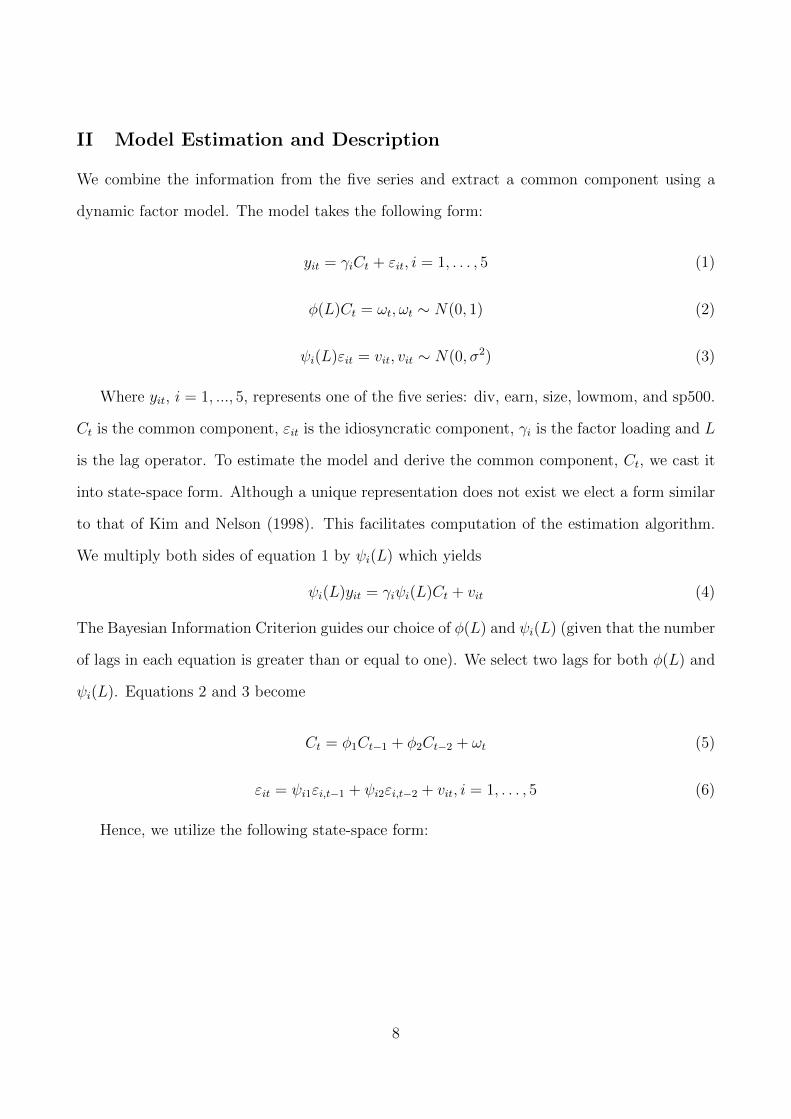
II Model Estimation and Description

We combine the information from the five series and extract a common component using a

dynamic factor model. The model takes the following form:

yit = γiCt + εit, i = 1, . . . , 5 (1)

φ(L)Ct = ωt, ωt ∼ N(0, 1) (2)

ψi(L)εit = vit, vit ∼ N(0, σ2) (3)

Where yit, i = 1, ..., 5, represents one of the five series: div, earn, size, lowmom, and sp500.

Ct is the common component, εit is the idiosyncratic component, γi is the factor loading and L

is the lag operator. To estimate the model and derive the common component, Ct, we cast it

into state-space form. Although a unique representation does not exist we elect a form similar

to that of Kim and Nelson (1998). This facilitates computation of the estimation algorithm.

We multiply both sides of equation 1 by ψi(L) which yields

ψi(L)yit = γiψi(L)Ct + vit (4)

The Bayesian Information Criterion guides our choice of φ(L) and ψi(L) (given that the number

of lags in each equation is greater than or equal to one). We select two lags for both φ(L) and

ψi(L). Equations 2 and 3 become

Ct = φ1Ct−1 + φ2Ct−2 + ωt (5)

εit = ψi1εi,t−1 + ψi2εi,t−2 + vit, i = 1, . . . , 5 (6)

Hence, we utilize the following state-space form:

8

Measurement Equation:

y∗1t

y∗2t

y∗3t

y∗4t

y∗5t

=

γ1 −γ1ψ11 −γ1ψ12

γ2 −γ2ψ21 −γ2ψ22

γ3 −γ3ψ31 −γ3ψ32

γ4 −γ4ψ41 −γ4ψ42

γ5 −γ5ψ51 −γ5ψ52

Ct

Ct−1

Ct−2

+

v1t

v2t

v3t

v4t

v5t

(7)

Which in matrix form becomes

(yt = Hβt + vt)

Where y∗it = yit − ψi1yi,t−1 − ψi2yi,t−2 as in the left hand side of equation 4.

E(vtv′t) = R =

σ21 0 0 0 0

0 σ22 0 0 0

0 0 σ23 0 0

0 0 0 σ24 0

0 0 0 0 σ25

(8)

Transition Equation:

Ct

Ct−1

Ct−2

=

φ1 φ2 0

1 0 0

0 1 0

Ct−1

Ct−2

Ct−3

+

ωt

0

0

(9)

Equation 9 can be written in matrix form as

(βt = Fβt−1 + et)

E(ete′t) =

1 0 0

0 0 0

0 0 0

(10)

We estimate the model using the Bayesian multimove Gibbs-sampling approach based on

9

Carter and Kohn (1994) and Kim and Nelson (1998) instead of the typical maximum likelihood.

In the classical maximum likelihood approach inferences about the state vector are based on the

estimated parameters. This is critical since the state vector contains the common component

representing the sentiment index. In essence, the classical procedure forces the researcher

to treat the estimated maximum likelihood parameters as true values when calculating the

estimates for the state vector. We circumvent this issue through the Bayesian technique which

allows us to jointly estimate the state vector and the model’s parameters. To implement the

estimation algorithm we use the MCMC Gibbs-sampling method. We run the algorithm 10,000

times and drop the first 2000 iterations. For further explanation of these techniques see Kim

and Nelson (1998, 1999).

III Empirical Results

Table II shows the estimated parameters. As mentioned above, the factor loading for variable

i is γi. The factor loadings are all have the expected positive sign. Furthermore, the loadings

for div, earn, size, and lowmom are much higher than the loading for sp500. This results is not

surprising. Based on prior research we expect the div, earn, size, and lowmom series to more

directly capture sentiment.

[Insert table II here.]

We interpret the the common component, Ct, as a sentiment index for the stock market.

We plot the series versus market weighted returns in figure 1. The sentiment index is noisy but

there appears to be large aberrations in the index around times of high or low sentiment. For

example, volatility is high around the tech bubble in 2000. The sentiment index is much more

volatile than the market weighted returns during these sentiment episodes. To gain insight into

the results of the index we filter the series using the HP filter with the smoothing parameter,

λ = 150.10 We present the augmented series in figure 2.

[Insert figures 1 and 2 here.]

The index appears to be correlated with bear markets and leads NBER recessions. We define

10Larger values of λ translate into more smoothing.

10

a bear market as a 20 percent or more drop in the overall market for at least a two month

period. Also, the index levitates after many bear markets. For example, the index jumps

following the tech crash in 2000 and the credit crash of 2008. This result is not surprising

as firms most affected by sentiment produce their greatest returns immediately after a bear

market. Using the filtered series makes the differences between market weighted returns and

our index even more pronounced: our index captures major sentiment episodes such at the late

1960s and 1990s while the market weighted returns do not.

Next we conduct an exercise to determine if our index is robust to macroeconomic and

business cycle indicators. In this regard, we use a process similar to Baker and Wurgler (2006).

For each component of our index we control for (regress out) growth in industrial production,

consumer durables and consumer nondurables. We also control for the one month Treasury

rate and NBER recessions.11 We then re-compile our index to develop a “macro-orthogonalized

index” using the augmented components. If our original index and the macro-orthogonalized

index are similar then we contend that our methodology is robust to business cycle indicators.

The correlation between our original index and the macro-orthogonalized index is 0.993. There

is little difference between our original index and the macro-orthogonalized index. Hence, for

the remainder of the paper we only consider the original index.

Baker and Wurgler (2006, 2007) and Gluskov (2006) among others conclude that smaller

stocks are more affected by sentiment. As a robustness check we use our index to calculate

the sentiment beta for ten portfolios based on size. The sentiment beta is analogous to the

popular market beta. Hence, a higher sentiment beta implies that a portfolio is more affected

by sentiment. We follow Baker and Wurgler (2007) and control for market weighted returns.

Based on prior research, we expect that portfolios consisting of smaller firms should have higher

sentiment betas. Table V shows our results. Our findings correspond to our expectations:

portfolios made up of smaller stocks have larger sentiment betas. We discuss the relationship

between varying risk and our sentiment index below.

11We obtained growth in industrial production, consumer durables and consumer nondurables from theFRED economic database. The series IDs are INDPRO, IPDCONGD, and IPNCONGD, respectively. Theone-month Treasury rate is available from Kenneth French’s Data library.

11

[Insert table V here.]

We plot our index versus Baker and Wurgler’s (2006, 2007) index in figure 3. In contrast

to their index, our sentiment index peaks at the conclusion of speculative episodes and crashes

as bear markets take hold. For example, our index peaks before the bear markets beginning in

1966M02, 1968M11, 1981M01, 1987M08, and 2000M03. In comparison, Baker and Wurgler’s

index peaks or remains high through the bear markets in the late 1960s, early 1980s and early

2000s.

Practitioners often consider the VIX volatility index as a “market fear gage.” In other

words, the VIX index rises along with investor fear. We expect that sentiment indexes should

be negatively correlated with the VIX index: when fear is high sentiment should be low, and

vice versa. However, we should not expect strong correlation with the VIX index. As stated

by Whaley (2000), “VIX is more a barometer of investors’ fear of the downside than it is

a barometer of investors’ excitement (or greed) in a market rally.” We can use the VIX

index as a robustness check for the performance of sentiment measures. We opt to use the old

formula for the volatility index which is traded under the symbol VXO. VXO contains a longer

sample than the VIX index.12 We compare our raw sentiment index, Baker and Wurgler’s

sentiment index and VXO volatility for a common sample ranging from 1986M01 to 2007M12.

As expected, our sentiment index and the VXO volatility index are negatively correlated. The

correlation coefficient between our index and VXO is -0.14. In comparison, the correlation

between Baker and Wurgler’s sentiment index and the VXO volatility index is positive at 0.29.

The positive correlation between Baker and Wurgler’s index and the VXO index contradicts

our expectations.

Baker and Wurgler (2006) document anecdotal evidence of stock market sentiment com-

prised from a number of sources between 1961 and 2002. Using the filtered index in figure 2,

we find that our sentiment index generally coincides with their findings. First, Baker and Wur-

gler (2006) find a bubble during 1961. Our index reaches a local maximum during this period

12For the calculation of the VIX index and its comparison with VXO see http://www.cboe.com/micro/

vix/vixwhite.pdf. The correlation coefficient between VIX and VXO over our sample is 0.988

12

and then falls as the bear market ensues in 1962. Also, Baker and Wurgler (2006) state that

sentiment jumps in 1967 and 1968. Our sentiment index rises sharply during the late 1960s

before peaking just prior to the bear market beginning in late 1968. Low sentiment ensued as a

bear market set in between late 1968 and 1971. Our sentiment index shows a crash during this

episode. Baker and Wurgler (2006) document bubbles in 1977 and 1978 and again in the first

half of 1983. Our index shows spikes around these bubbles. These periods are associated with

the end of bear markets. It may difficult to determine whether the rises in our index are due

to the aforementioned bubbles or just a typical jump that follows many bear markets. Baker

and Wurgler (2006) conclude that sentiment is high through the mid 1980s and then dissipates

in 1987 and 1988. Our index climbs following the end of the bear market in 1982 until the

stock market crash in 1987. After this crash however, our index moves upward through the

recession and bear market of 1990. Our index shows a dramatic drop at the beginning of 1997

corresponding to the time of the Asian Financial crises. Our sentiment index peaks in the late

1990s as extreme optimism created by the tech bubble gripped the markets and then crashes as

the bubble burst. Sentiment falls again prior to the credit crisis in 2008 and rises dramatically

at the end of our sample as a bull market took hold beginning in March of 2009.

Using both the HP filtered series with the smoothing parameter, λ, equal to 150 and the

unfiltered series we run regressions to determine the in-sample predictive value of the sentiment

index. We lag the sentiment index by one period. We also control for the three factors, MKT ,

HML and SMB of Fama and French (1993) and a momentum factor as is typical in the

finance literature. If one of the factors is used as the dependent variable we do not include it

in our set of regressors. We run separate regressions using the MKT factor, the HML factor,

the SMB factor and the momentum factor as dependent variables. We will also conduct a fifth

regression where the dependent variable is the market weighted return, denoted MKT 1. Let

us denote the sentiment series as SENT and the momentum factor as UMD. Let the variable

Zt represent any of the five regressands. The regression equation becomes:

Zt = α + β1SENTt−1 + β2MKTt + β3SMBt + β4HMLt + β5UMDt + εt (11)

13

We provide the regression results for the filtered and unfiltered sentiment series in tables

III and IV, respectively. The true distribution of the errors is likely non-normal. Hence, we

calculate the bootstrapped standard errors as in Stambaugh (1999). The size component used

to develop our index is similar to the Fama and French (1993) SMB factor.

[Insert tables III and IV here.]

We first consider the results when the sentiment index is filtered. The regression coefficient

on SENTt−1 is positive and significant when MKTt or MKT 1t is the dependent variable. A

positive regressor on sentiment implies that an increase in sentiment at time t − 1 relates to

an increase in the overall market return in time t. Moreover, these coefficients are above one

which may suggest a strong relationship between the market returns and the sentiment index.

When the dependent variable is HML or UMD the coefficient on SENTt−1 is negative and

insignificant.

Next we examine the results where the sentiment index is not filtered. When the dependent

variable is either MKT or MKT 1, the coefficient corresponding to the sentiment index becomes

insignificant but the sign remains positive. It is possible that the noise that we filtered out in

the sentiment index is related to the noise in the other Fama-French factors. This may explain

the smaller coefficient and lack of significance in this case. Additionally, for the regressions

where HML and UMD are the dependent variables the sign for the coefficient on SENTt−1

becomes positive and significant.

When SMB is the dependent variable the β for the sentiment index is positive and signif-

icant for both the filtered and unfiltered index. It is much larger when the sentiment index

is filtered. Baker and Wurgler (2006) also construct a sentiment index and run a similar re-

gression using the SMB factor as the dependent variable. They find the coefficient on their

sentiment index to be negative and significant. Their sample contained data from 1963M01

to 2001M12 while our sample draws from 1951M07 to 2009M08. Also, they use significantly

different components for their index.

The positive coefficients on the sentiment index when the dependent variable is MKT and

MKT 1, among others, may support the idea of sentiment driven bubbles. An increase in

14

sentiment at time t− 1 relates to an increase in the market averages (or other dependent vari-

ables) at time t. Hence, broad increases of sentiment over time translate into higher aggregate

returns. These results contradict the empirical results of Baker and Wurgler (2006, 2007) but

coincide with the theoretical results of Abreu and Brunnermeier (2003). Baker and Wurgler

contend that high sentiment implies lower future returns. Abreu and Brunnermeier conclude

that rational arbitrageurs have a profit incentive to ride sentiment bubbles. In other words,

they find that rational arbitrageurs may not necessarily sell out if sentiment is high. Lutz

(2010d) uses ep10 as a measure of sentiment. For sentiment portfolios based on earnings and

dividends he found that rising sentiment relates to rising returns. One must be careful when

interpreting these results as correlation does not necessarily imply causation. As noted in the

introduction, in the literature the affect of sentiment on a cross-section of stocks is mixed.

Next we examine the relationship between our sentiment index and risk. The rational-based

Capital Asset Pricing Model (CAPM) contends that riskier portfolios should always have a

higher expected return. The popular beta determines the portfolio’s risk. Hence, portfolios

with higher betas should earn higher expected returns. From this perspective, one may argue

that our sentiment index is just capturing varying degrees of risk rather than the effects of

sentiment. To study this issue we consider an exercise similar to that of Baker and Wugler

(2007). We form ten decile portfolios based on size.13 The first row in table V shows the market

beta for these portfolios. The results coincide with our expectations: the portfolios made up

of smaller stocks are riskier and have larger betas than those consisting of larger stocks. The

average returns, also depicted in table V, are higher for portfolios with larger betas. Hence, for

average returns the CAPM predictions hold. In addition, we examine portfolio returns when

sentiment is high in the previous month and when sentiment is low in the previous month.

Sentiment is low during the previous month if it is below the mean and vice versa for high

sentiment during the previous month. Table V and figure 4 show the results. When sentiment

is high during the previous month the CAPM’s effects become more pronounced: portfolios

with higher betas earn much higher returns. Furthermore, the high beta portfolios earn better

13Size portfolios are from Kenneth French’s data library.

15

than average returns while low beta portfolios earn below average returns. The results reverse

when sentiment is low during the previous month. In this case high beta portfolios earn much

lower returns than low beta portfolios. These results violate the CAPM predictions. Baker and

Wurgler (2007) label the graph in figure 4 as “the sentiment seesaw.” Not surprisingly, given the

above regression results, our empirical seesaw and Baker and Wurgler’s are inverses. However,

we both find that the CAPM fails to explain the results: for a given level of sentiment high

beta stocks earn lower returns. In Baker and Wurgler’s words, “This is a powerful confirmation

of the sentiment-driven mispricing view.”

[Insert figure 4 here.]

IV Out of Sample Forecasting

Now we examine the out of sample forecasting performance of the sentiment index outlined

in section II. We follow Timmermann (2008) and attempt to forecast one-step ahead market

weighted stock returns. Using market-weighted returns ensures that our results are robust to

both large and small firms.14 To avoid look-ahead bias we will not use the exact sentiment

index estimated in section III. Instead we re-estimate the model in section II for each in-sample

period considered.

To evaluate the forecasts we employ the mean-absolute error (MAE) and the out-of-sample

(OOS) R2 measure used in Campbell and Thompson (2007) and Goyal and Welch (2008). The

formula for the OOS R2 is

R2 = 1− MSEn

MSERWD

(12)

Where MSEn is the mean-squared error for model n and MSERWD is the mean-squared error

for the benchmark random walk plus drift. If the OOS R2 is positive then model n outperforms

the benchmark. We follow the literature and express the OOS R2 statistic as a percentage.

We consider several models to develop our forecasts. We have information available up to time

period t and hope to forecast returns at time t + 1. Let rt+1 represent returns for time t + 1

14Some authors also consider equal-weighted returns. However, these averages are biased towards small firmsand do not truly represent market averages.

16

and εt+1 represent an unpredictable white noise process.

The benchmark model we consider is the random walk plus drift:

rt+1 = β0 + εt+1 (13)

The forecast for this model is the unconditional mean. In out of sample forecasting exercises

researchers have struggled to outperform this benchmark on a consistent basis as evinced in

Timmermann (2008).

The next model we consider is a linear autoregressive model where lags of the market return

and the sentiment index represent the independent variables. The specification for this model

is as follows:

rt+1 = β0 +

p∑j=1

αjrt+1−j +

q∑j=1

βjSENTt+1−j + εt+1 (14)

The lags for p and q were chosen using the Bayesian Information Criterion (BIC). We force the

model to contain at least one independent variable. This ensures that the linear model differs

from the random walk plus drift. We discuss the performance of various autoregressive and

sentiment lags in section B.

We also consider two nonparmetric models:

rt+1 = m(SENTt) + εt+1 (15)

rt+1 = m(rt, SENTt) + εt+1 (16)

We estimate equation 15 using local liner least squares and equation 16 using local constant

least squares.

We also consider a NARX neural network which approximates an equation of the following

form in a non-linear fashion:

rt+1 = f(rt, rt−1, . . . , rt−p, SENTt, SENTt−1, . . . , SENTt−q) (17)

For our NARX forecast we consider a model with one hidden layer and one output layer. We

use ten neurons in the hidden layer. To train the network, we opt for Bayesian regulation.

This helps avoid overfitting. For more on Bayesian regulation see MacKay (1992) or Foresee

17

and Hagan (1997). We select the lengths of p and q by regressing the fitted values on the

actual data. This is standard practice in the neural network literature.

The last model that we entertain is a Generalized Regression Network. These models

contain a hidden radial basis layer and special linear layer. One advantage of these models

is that they can be trained rather quickly. To use this model we simply specify the market

weighted returns as the target vector and the SENTt−1 series as the input vector. For more

on Radial Basis Networks see Wasserman (1993).

Finally, we average the forecasts over all the models to form a combined forecast.

We consider both rolling window and recursive estimates of the sentiment index and our

forecasting models. The data generating process (DGP) for asset returns most likely changes

over time. Hence, there is a tradeoff between the recursive and rolling window methods. The

recursive procedure uses more information which may yield better estimation results of the

model parameters. A rolling window allows the model to adapt to changes in the DGP.

First, we consider a rolling window of ten years or 120 monthly observations. The first

forecast corresponds to 1970M01. For each window we estimate the sentiment index as outlined

in section II. Then we form the one-step ahead forecast for the various models discussed above.

The exact structural form of the sentiment index most likely changes over time. Thus, we

consider three different models relating to the different number of lags in for φ(L) and ψ(L) for

every window.15 We then average the results from these models to develop a single sentiment

index. We consider the index as an exogenous independent variable. Then we form the one-

step ahead forecast of market weighted returns. We present the results for the MAE and

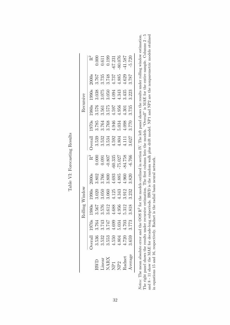
OOS R2 in the left panel of table VI. RWD is the random walk plus drift model. NP1 and

NP2 correspond to the non-parametric models in equations 15 and 16, respectively. Radnet

represents the radial basis neural network. Surprisingly, the linear model produces the lowest

MAE for the entire sample. This autoregressive model also performs better out of sample than

the benchmark random walk plus drift in the 1970 and 2000 subperiods. The NARX model

15We used one lag for φ(L) and one lag for ψ(L) for the first model, two lags for φ(L) and one lag for ψ(L)for the second, and two lags for both φ(L) and ψ(L) for the third.

18

performed well in the 1970s and 2000s but failed to outperform the benchmark model in the

overall sample. The rest of the models produced higher MAEs over the entire sample. Also,

the OOS R2 is positive for the linear model. This suggests that the linear model outperforms

the benchmark for the overall sample.

[Insert table VI here.]

Next, we estimate both the sentiment index and forecasting models recursively. Table VI

contains the results. In this case, the linear model outperforms the benchmark model by a

wider margin. In contrast to previous results, the NARX model outperforms the random

walk plus drift over the entire sample. The NARX model also beats the benchmark in all

subperiods except the 1990s. Furthermore, the NARX model produces a lower MAE under

recursive estimation. All other models fail to produce lower MAEs than the benchmark for all

subperiods. The average forecast outperforms the random walk plus drift for the 1970, 1980

and 2000 subperiods. The OOS R2 is positive for the NARX model under recursive estimation.

Lastly, the R2 increases significantly for the linear model.

The MAEs are generally equivalent or smaller when we estimate both the sentiment index

and the forecasting models using a rolling window. The average linear forecast is equivalent

under both approaches. The exceptions are the neural networks. They produce superior

forecasts under the recursive approach. The MAE for the benchmark random walk plus drift

is smaller under the rolling window approach. This may suggest that using a rolling window

allows the benchmark model to adjust to changes in the DGP.

A Bayesian Model Averaging

The true data generating process (DGP) of a series is often not known to researchers. As a

result, the researcher must consider a large set of models. Classical regression analysis utilizes

specific tools to choose the best model. This model is then used for prediction or forecasting.16

This approach fails to take into consideration the uncertainty surrounding the choice of the

optimal model. Neglecting this uncertainty may lead to errors in inference. Also, only using

16Such tools include R2 measures, Bayesian and Akaike information criterions, log-likelihood values, etc.

19

one model may disregard information contained in alternative specifications.

In the above forecasting section we combined out-of-sample predictions using a simple

average. Now we turn to more advanced mixing techniques. In particular, we employ Bayesian

model averaging (BMA). BMA takes into account the uncertainty regarding the true nature

of the process. There are two main ways implement BMA. The first method assumes that

there is one correct model but the researcher is ignorant to its true form. Raftery (1995) and

Hoeting et al. (1999) outline this use of BMA. Raftery et al. (2005) develop a dynamic BMA

procedure where the correct model changes from time period to time period. The dynamic

BMA technique draws the optimal specification from the weighted average over a given set

of models. Furthermore, this technique only requires the model forecasts. This makes it

convenient to average over linear and non-linear specifications. In essence, the dynamic BMA

procedure produces an optimal forecast by mixing over the forecasts from a given set of models.

In all likelihood, the DGP of stock returns changes over time. Also, we want to combine the

linear and non-linear models depicted above. Hence, we select the dynamic BMA approach.

Following the notation of Raftery et al. (2005), the BMA predictive pdf is given by

p(y|f1, . . . , fK) =K∑k=1

wkgk(y|fk) (18)

Where y is the quantity to be forecast, K is the number of models, wk is the weight applied to

each model, and gk(·) is an assumed probability distribution. wk is the posterior probability.

We interpret gk(y|fk) as the pdf of y conditional on fk given that model k produced the best

forecast over the training period.

We form the log-likelihood function based on the distribution in equation 18. We specify a

functional form for gk(y|fk). Since this is a finite mixture model we can apply the EM algorithm

to maximize the likelihood function. Before we execute the EM algorithm we must also choose

the length of the training period. To accommodate the changes in the DGP over time we use

a rolling window of forecast data to estimate the likelihood function. Shorter rolling windows

allow the model to adjust quickly to changes in the structure of the process. Longer windows

use more information. This yields better estimation of model parameters. Researchers widely

20

believe stock returns follow a distribution with thick tales such as the t-distribution. Despite

this fact, we consider the normal distribution for gk(·). As noted by Peel and McLachlan

(2000), mixing over the t-distribution simply produces less extreme results than the normal

distribution. Hence, using the normal distribution instead of the t-distribution allows us to

add larger weights to better forecasts and further punish poor performing models.17

Raftery et al. (2005) note that the weights calculated by the BMA technique consider the

performance over the training period and the correlation of the forecasts. A model may obtain

a larger weight than one might expect if its forecasts are uncorrelated with others. Table VII

shows the correlations of the forecasts. The random walk plus drift, linear and NARX models

are all highly correlated with a coefficient around 0.65. The non-parametric models are highly

correlated with each other but much less so with other models. The Radnet model is almost

completely uncorrelated with the others. The non-parametric and the Radnet models perform

extremely poorly out-of-sample. Yet the dynamic BMA process will still place significant

weights on their forecasts due to their small correlation with the other models. Hence, we

drop these specifications and only average over the random walk plus drift, the linear and the

NARX models.

We only consider the forecasts from the random walk plus drift, the linear model and

the NARX model under a rolling window.18 We discard the first 60 observations to use as

verification. This implies we are eliminating half of the 1970s from our out-of-sample exercise.

As noted in table VI, the 1970s were a subperiod where both the linear model and the NARX

model outperformed the benchmark. Hence, not using the first half of the 1970s will negatively

affect our results. Despite this handicap, we do not change the out-of-sample period to avoid

data mining.

The left panel of table VIII shows the results when we average over the random walk plus

drift, linear and NARX models. The first column corresponds to the length of the training

17Results for the t-distribution are available upon request. Using the t-distribution did not improve ourresults.

18Forecasts under a rolling window produced lower MAEs for the random walk plus drift. Hence, the randomwalk plus drift under a rolling window is a more difficult benchmark to beat.

21

period. In columns 2 - 4 we show the posterior weights and their standard deviations in

parentheses. We use the OOS R2 statistic to judge forecast performance. The mean of the

posterior weight for all the models hovers around 1/3. However, the weight on the random walk

plus drift is usually the highest followed by the linear and NARX models. The BMA forecasts

outperform the the benchmark random walk plus drift for all training lengths considered. The

best performing model uses 20 training periods and produces an R2 of 0.52.

[Insert table VIII here.]

We find that the standard deviations for the posterior weights are quite large. Hence, the

optimal forecasting model changes drastically over time. We plot the posterior weights in

figure 5 using a training length of 35 periods. We also shade bear markets. However, this

shading can be misleading. Recall that BMA calculates the posterior weights based on prior

training lengths. For this case, a posterior weight describes the forecasting performance over

the previous 35 training periods. For example, the random walk plus drift model commands a

large posterior weight in the early 2000s. This suggests that the random walk plus drift was

the top performer in the late 1990s.

[Insert figure 5 here.]

As mentioned above, the BMA process will add extra weight to forecasts that are uncorre-

lated with others. When all the forecasts considered are correlated at the same level, however,

we can interpret the BMA posterior weights as out of sample model performance over the

training period. This is the case for the random walk plus drift, linear and NARX models.

Hence, mean weights for the three models imply similar out of sample forecasting performance

for the random walk plus drift and linear frameworks and slightly worse performance for the

NARX model.

Next, we apply the BMA technique over just the linear and random walk plus drift models.

The right panel in table VIII holds the results. The posterior weight for the random walk plus

drift hovers around 0.55. This compares to a weight of about 0.45 for the linear model. These

results suggests that random walk plus drift usually provides a slightly better forecast. The

standard deviations for posterior weights are quite large. Hence, the optimal model changes

22

over time. The BMA forecast outperforms the benchmark except when we use a training length

of ten periods. Furthermore, the largest R2 is 0.85 in this case. In comparison, the largest R2 is

0.52 when we average or the random walk plus drift, the linear and the NARX models. Thus,

averaging over just the random walk plus drift and the linear model improves performance.

B Two-stage Bayesian Model Averaging

While we mix forecasts in the above BMA procedure from various models we use conven-

tional econometric methods to determine their specifications. This neglects the uncertainty

surrounding the choice of model specifications. To account for this uncertainty and combine

the forecasts from the various models we employ a method we call two-stage Bayesian model

averaging (2SBMA). Before we describe this method let us introduce basic terminology to

facilitate the discussion.

Let a model be a generic functional representation of the process and a specification be

a single representation of a model. For example, the models will be the random walk plus

drift, linear and NARX. For the linear model a given specification will be a certain number of

autoregressive or sentiment lags. The random walk plus drift model only has one specification

(corresponding to zero autoregressive and sentiment lags). The linear and NARX models have

potentially an infinite number of specifications.

The BMA technique of Raftery et al. (2005) allows for different models but the procedure is

difficult to implement if models have different specifications. The 2SBMA approach augments

the standard BMA technique to allow models to have different specifications. More explicitly,

the 2SMBA approach requires two steps: (1) apply the BMA procedure for each model over all

considered specifications; and (2) apply the BMA approach again over all models. In essence, we

average over all specifications for each model and then over all models. The 2SBMA technique

also allows the researcher to discard specifications that are known to perform poorly or add

specifications which may forecast well for some models but not others. Overall, the 2SBMA

approach is a simple and flexible framework to combine forecasts. The 2SMBA technique also

23

allows researchers to incorporate linear and non-linear models and their various specifications.19

In the first stage, the optimal number of training periods may differ across models. Thus, we

may want to use different training lengths for different models in the first stage. For example,

table IX shows that about 30 training periods are appropriate for the linear model and table X

shows that 60 training periods are optimal for the NARX neural network. Ideally, in the second

stage we would use the forecast that corresponds to 30 training lengths for the linear model and

60 training lengths for the NARX network. Unfortunately, blindly using these training lengths

would lead to look-ahead bias. To circumvent this issue, in stage one we record the OOS R2

for each model and all training lengths up to time period t. We choose the forecast from each

model that produces the highest R2. Then we conduct the second stage of the process to make

the 2SBMA forecast for time t + 1. This process allows us to use the optimal forecast from

stage one in stage two.

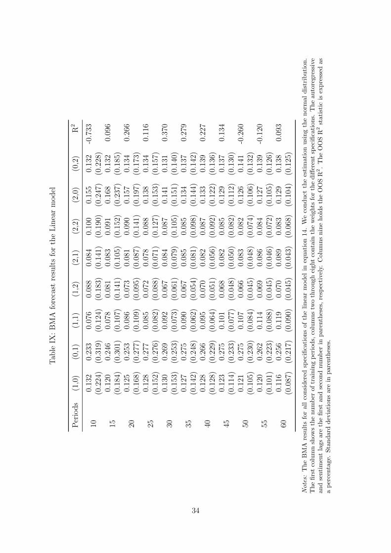
Tables IX and X show the results from the first stage of the 2SMBA process for the linear

and NARX models, respectively. We do not need to consider the random walk plus drift model

in the first stage as it only has one specification. We use the normal distribution for the mixing

process. As before, we use the first 60 forecasts as verification. For the linear model, the BMA

procedure places the highest weight on the specification where (p = 0, q = 1).20 This weight

is twice as large as the posterior probability for any other specification. The mixing process

also places significant weight on the specifications where (p = 1, q = 0), (p = 2, q = 0) and

(p = 0, q = 2). The standard deviations for the posterior weights are large. This indicates

that the optimal specification changes over time. Additionally, using a training length of 30

periods produces the largest OOS R2. The BMA forecast for the linear model beat the random

walk plus drift by a larger margin than the linear model in section IV. Furthermore, the BMA

forecast for the linear model outperforms the benchmark when we use 15-45 or 60 training

periods.

[Insert tables IX and X here.]

19One could also average the BMA forecasts in some manner over the various training periods. An equalweighted average over different training periods would be easy to implement.

20p and q are the autoregressive and sentiment lags, respectively. See equation 14 for the linear model.

24

The posterior weights for the NARX model are relatively equal across all specifications and

training periods. The BMA forecast for the NARX model outperforms the benchmark when

20, 25, 35, 40, 45, 50, 55 and 60 training periods are used.21

The left panel in table XI displays the second stage the the 2SBMA process. In this case

we average over the random walk plus drift, linear and NARX models. The largest posterior

weight belongs to the random walk plus drift model, followed by the linear model. The 2SBMA

process places the lowest weight on the NARX model. The R2 is positive when the training

length is set to 15 - 45 or 60 periods.

[Insert table XI here.]

We also consider the 2SMBA approach over just the linear and random walk plus drift

models. The right panel of XI shows the results. Using only the linear and random walk plus

drift models produces even better forecasts. All of the R2’s are extremely large in magnitude

and above 1.5 percent. When we use 10 training lengths, the OOS R2 is 2.319. The 2SBMA

forecasts are among the best in our study.

We use 120 observations for verification in the 2SBMA approach. This implies that we

do not include the 1970s in our 2SBMA forecasts. Recall that the 1970s were a period where

both the linear and NARX models outperformed the benchmark. Hence, our results may be

negatively affected. Yet the 2SBMA forecasts still beat the random walk plus drift. We do not

adjust the sample to include the 1970s to avoid data mining.

The drawback of the 2SBMA approach compared to the BMA process is that it requires

twice as many observations for verification. This cost is minimal, however, when a large time

series of forecasts is available (as it is in our case) or when the researcher is mostly concerned

with predicting future, unobserved values. Considering shorter training windows also helps

substantially reduce this cost.

21When only considering autoregressive lags, instead of the NARX framework we use a time delayed neuralnetwork. Also, when the independent variables are only lags of the sentiment index we use a standard feed-forward neural network.

25

C Comparison with other stock market forecasts

There has been a long debate over the predictability of asset returns. Pearson and Timmermann

(1995) conclude that return predictability is limited to certain subperiods. Campbell and

Thompson (2007) find that some variables exhibit small out-of-sample superiority compared

to a recursively estimated random walk plus drift. However, they restrict the signs of the

regression coefficients. They also conclude that a variable loses its predictive power over time.

Campbell and Thompson also find that returns are least predictable after 1980. Our 2SBMA

models produce large and positive R2’s after 1980. Goyal and Welch (2008) contend that returns

are not forecastable using typical variables. Furthermore, Timmermann (2008) considers a

battery of models and regressors. Using market-weighted returns all of his models fail to

outperform the random walk drift under a rolling window. Using recursive estimation he

finds that only an equal-weighted average of forecasts outperforms the benchmark random

walk plus drift. He concludes models can at best achieve local predictability. Lutz (2010d)

considers Baker and Wurgler’s sentiment index, ep10, and the VIX volatility index as exogenous

variables.22 He uses a number of unrestricted and restricted models. Lutz (2010d) finds that

only the VIX volatility index is able to forecast market weighted using a NARX network. Our

results support the proposition that stock returns are forecastable. Controlling for sentiment,

we use both a rolling window and recursive estimation. We find individual and average forecasts

that outperform the benchmark under both a rolling window and recursive approach.23

V Sentiment Cycles

Using the index outlined in sections II and III we date cycles in sentiment. To our knowledge,

no other work has quantitatively chronicled sentiment episodes.24 We apply a modified Bry-

Boshan algorithm to date sentiment cycles. The Bry-Boschan algorithm is a set of conditional

22See footnote 4 for an explanation of the ep10.23As previously stated, we find that the average MAE under the rolling window is lower than under recursive

estimation for the random walk plus drift. Hence, superior performance over the random walk plus drift usinga rolling window would be much more useful to practitioners.

24Baker and Wurgler (2006) document anecdotal periods of sentiment. Their approach is qualitative. Wecompare our sentiment index to these accounts in section III.

26

rules to find local highs and lows in a series. We modify the window lengths and the and cycle

durations in the algorithm to fit our noisy data. We also require that the magnitude of each

phase be greater than 1.5 standard deviations of the entire index. This ensures that small

blips are not recorded as peaks or troughs in sentiment. Appendix A shows the exact set of

rules we use for the algorithm. Table XII and figure 6 show the results. The shaded areas

in the figure represent peak to trough episodes in agent sentiment. The modified algorithm

appears to capture the dynamics of the index. Furthermore, sentiment usually peaks prior to

bear markets. This is the case for the bear markets that began in 2008, 2000, 1987, 1981, 1976,

1968, 1966 and 1957. Our algorithm does not record a peak in sentiment prior to the bear

market in 1961. Also, sentiment peaks just after the light bear market in the early 1990s. The

algorithm also records many false alarms. These usually occur as sentiment levitates following

bear markets. For example, the algorithm records peaks following the bear markets in 2002,

1990, 1982 and 1957. As noted above, these results are not that surprising since the stocks

most affected by sentiment produce their greatest returns following bear markets. Clearly,

there is a correlation between sentiment and bear markets. However, more study is needed to

determine if a causal relationship exists and how this affects practitioners and policymakers.

[Insert table XII and figure 6 here.]

VI Conclusion and further discussion

Using a dynamic factor model and Bayesian estimation we construct an index for stock sen-

timent using only market return data. This index generally matches episodes of sentiment

bubbles. We run in sample regressions using our index and find a relationship between increas-

ing sentiment and increasing stock returns. This result supports the idea of sentiment driven

bubbles and crashes. In an out-of-sample forecasting exercise we find that conditioning on

sentiment allows us to outperform a benchmark random walk plus drift model over our sample

period. The results are robust for rolling window and recursive estimation. To our knowledge,

this result is new to the literature. These findings support the notion that sentiment affects

a broad cross section of stocks. Furthermore, we find that sophisticated averaging techniques,

27

such as Bayesian model averaging (BMA), can enhance forecasting performance. In this re-

gard, we develop a simple extension called two-stage Bayesian model averaging (2SBMA). This

technique allows researchers to combine forecasts from different models all with different spec-

ifications. 2SBMA produces more accurate predictions than the standard BMA approach in

our forecasting exercise. Lastly, we date cycles in sentiment. We find that sentiment cycles

often lead bear and bull markets. Future research may investigate how sentiment cycles affect

bull and bear markets, how sentiment affects stocks in aggregate, and what role does sentiment

play in the formulation of bubbles.

A Appendix: Procedure For Determination of Turning Points

1. Remove outliers from the data and replace them using the Spencer curve.

2. Determination of initial turning points in raw data

(a) Determination of initial turning points in raw data by choosing local peaks (troughs)as occurring when they are the highest (lowest) values in a window 12 months oneither side of the date.

(b) Enforcement of alternation of turns by selecting highest of multiple peaks (or lowestof multiple troughs)

3. Censoring operations (ensure alternation after each)

(a) Elimination of turns within 6 months of the beginning and end of the series

(b) Elimination of peaks (or troughs) at both ends of the series which are lower (orhigher) than values closer to the end

(c) Elimination of cycles whose duration is less than 24 months

(d) Elimination of phases whose duration is less than 4 months or whose magnitude issmaller than 1.5 standard deviations of the sentiment index.

4. Statement of final turning points

B Appendix: Tables and Figures

28

Table I: The correlation of sentiment components

Div Earn Size Lowmom

Div 1 0.86 0.8 0.79Earn 0.86 1 0.73 0.69Size 0.8 0.73 1 0.62Lowmom 0.79 0.69 0.62 1

Table II: Bayesian posterior distribution.

Variable Mean Med Std

φ1 0.233 0.234 0.014φ2 0.009 0.009 0.014γ1 3.660 3.657 0.092ψ11 0.012 0.012 0.055ψ12 0.006 0.006 0.055σ21 0.561 0.555 0.121γ2 3.778 3.777 0.119ψ21 -0.168 -0.170 0.043ψ22 0.025 0.025 0.042σ22 4.809 4.794 0.287γ3 6.282 6.274 0.237ψ31 0.195 0.195 0.041ψ32 -0.074 -0.074 0.041σ23 24.211 24.182 1.358γ4 3.233 3.230 0.120ψ41 0.040 0.040 0.040ψ42 0.053 0.054 0.041σ24 6.414 6.401 0.374γ5 1.324 1.321 0.118ψ51 0.220 0.220 0.039ψ52 -0.055 -0.054 0.037σ25 9.728 9.683 0.534

Notes: See section II for a description of the model. i = 1, . . . , 5 represent the five series, div, earn, size,lowmom and sp500, respectively. γi is the coefficient on the common component in equation 1. φi are thecoefficients on lags of the common component in equation 2. ψi are the coefficients on lags of the idiosyncraticcomponent in equation 3.

29

Table III: Regression Results for filtered sentiment

Dependent Var α SENTt−1 MKTt SMBt HMLt UMDt

MKTt0.7763* 1.3788* - 0.247* -0.4141* -0.1764*(0.000) (0.0008) (0.000) (0.000) (0.000)

HMLt0.616* -0.2702 -0.1681* -0.1453* - -0.1486*(0.000) (0.1549) (0.000) (0.000) (0.000)

UMDt0.9961* -0.2314 -0.1704* -0.0478 -0.3536* -(0.000) (0.2969) (0.000) (0.186) (0.000)

SMB0.2113* 1.6994* 0.1168* - -0.1692* -0.0234(0.0283) (0.000) (0.000) (0.000) (0.1937)

MKT 1t

1.1706* 1.272* - 0.2478* -0.4118* -0.1742*(0.000) (0.0008) (0.000) (0.000) (0.000)

Notes: Results for the regressions based on equation 11. For these results the sentiment index is filtered usingthe HP filter (λ = 150). Bootstrapped p-values are in parentheses. An asterisk means the variable is significantat the five percent level.

Table IV: Regression results for raw sentiment.

Dependent Var α SENTt−1 MKTt SMBt HMLt UMDt

MKTt0.7759* 0.0564 - 0.2866* -0.4287* -0.1831*(0.000) (0.3498) (0.000) (0.000) (0.000)

HMLt0.6242* 0.1686* -0.171* -0.1585* - -0.1524*(0.000) (0.0358) (0.000) (0.000) (0.000)

UMDt1.0053* 0.3986* -0.1725* -0.0686* -0.3599* -(0.000) (0.0024) (0.000) (0.097) (0.000)

SMB0.2135* 0.272* 0.1386* - -0.1922* -0.0352*(0.0259) (0.0045) (0.000) (0.000) (0.093)

MKT 1t

1.1696* 0.0363 - 0.2849* -0.4249* -0.18*(0.000) (0.4016) (0.000) (0.000) (0.000)

Notes: Results based on equation 11. Bootstrapped p-values are in parentheses. An asterisk means the variableis significant at the five percent level.

30

Tab

leV

:10

Siz

eP

ortf

olio

s

Lo

10D

ecile2

Dec

ile3

Dec

ile4

Dec

ile5

Dec

ile6

Dec

ile7

Dec

ile8

Dec

ile9

Hi

10

Bet

a1.

0823

1.16

251.

1646

1.13

811.

1283

1.08

301.

0887

1.07

461.

0036

0.93

79Sen

t-b

eta

3.27

362.

3234

1.72

751.

3755

1.05

720.

7079

0.49

860.

2850

-0.0

728

-0.4

899

Hig

hSen

t t−1

2.09

141.

6304

1.51

321.

3974

1.32

801.

1227

1.20

071.

0585

0.95

590.

7514

Ave

rage

1.16

641.

1307

1.17

381.

1243

1.14

331.

0821

1.09

161.

0468

1.00

490.

8787

Low

Sen

t t−1

0.38

350.

7022

0.87

430.

8822

0.97

561.

0354

0.98

371.

0196

1.02

940.

9692

Notes:

Th

em

arke

tb

eta

and

senti

men

tb

eta

for

the

por

tfoli

os

are

inro

ws

1an

d2.

Row

3h

old

sth

eav

erage

month

lyre

turn

wh

ense

nti

men

tw

as

hig

hin

the

pre

vio

us

mon

th,

row

4h

old

sth

eav

erag

em

onth

lyre

turn

over

the

wh

ole

sam

ple

an

dro

wfi

veh

old

sth

eav

erage

month

lyre

turn

when

senti

men

tw

as

low

duri

ng

the

pre

vio

us

mon

th.

31

Tab

leV

I:F

orec

asti

ng

Res

ult

s

Rol

ling

Win

dow

Rec

urs

ive

Ove

rall

1970

s19

80s

1990

s20

00s

R2

Ove

rall

1970

s19

80s

1990

s20

00s

R2

RW

D3.

536

3.76

43.

567

3.02

03.

802

0.00

03.

539

3.78

53.

576

3.03

83.

767

0.00

0L

inea

r3.

532

3.74

33.

576

3.05

03.

766

0.09

13.

532

3.76

43.

561

3.07

53.

735

0.61

1N

AR

X3.

553

3.74

73.

612

3.06

03.

800

-0.8

073.

534

3.76

83.

575

3.05

03.

748

0.19

9N

P1

4.55

04.

699

4.68

84.

125

4.69

3-6

0.33

54.

592

4.94

64.

597

4.09

44.

737

-67.

231

NP

24.

804

5.03

44.

956

4.34

34.

885

-75.

027

4.80

45.

034

4.95

64.

343

4.88

5-8

0.07

6R

adnet

4.72

04.

703

5.31

23.

912

4.96

0-8

4.75

84.

111

4.09

84.

301

3.43

54.

629

-41.

587

Ave

rage

3.65

93.

773

3.81

83.

232

3.82

0-6

.766

3.62

73.

770

3.73

53.

223

3.78

7-5

.720

Notes:

Th

em

ean

abso

lute

erro

ran

dth

eO

OS

R2

for

the

mod

els

ou

tlin

edin

sect

ion

IV.

Th

ele

ftp

an

elsh

ows

the

resu

lts

un

der

roll

ing

win

dow

esti

mati

on

.T

he

righ

tp

anel

show

sth

ere

sult

su

nd

erre

curs

ive

esti

mati

on

.T

he

firs

tco

lum

nli

sts

the

mod

els.

“O

vera

ll”

isM

AE

for

the

enti

resa

mp

le.

Colu

mn

s2

-5

and

8-

11sh

owth

eM

AE

for

dec

ade-

lon

gsu

bp

erio

ds.

RW

Dis

the

ran

dom

walk

plu

sd

rift

mod

el.

NP

1an

dN

P2

are

the

non

pare

met

ric

mod

els

otu

lin

edin

equ

atio

ns

15an

d16

,re

spec

tivel

y.R

adn

etis

the

rad

ial

basi

sn

eura

ln

etw

ork

.

32

Table VII: Forecast correlations.

RWD Linear NARX NP1 NP2 Radnet

RWD 1.000 0.682 0.631 0.117 0.106 0.036Linear 0.682 1.000 0.577 0.436 0.465 0.105NARX 0.631 0.577 1.000 0.240 0.245 0.078NP1 0.117 0.436 0.240 1.000 0.960 0.062NP2 0.106 0.465 0.245 0.960 1.000 0.061Radnet 0.036 0.105 0.078 0.062 0.061 1.000

Notes: RWD is the random walk plus drift model. NP1 and NP2 are the nonparemetric models otulined inequations 15 and 16, respectively. Radnet is the radial basis neural network.

Table VIII: BMA Forecast Results

RWD, Linear, NARX RWD, Linear

Periods RWD Linear NARX R2 RWD Linear R2

100.389 0.334 0.277 0.017 0.531 0.469 -0.103

(0.327) (0.316) (0.293) (0.299) (0.299)

150.382 0.302 0.316 0.479 0.536 0.464 0.502

(0.279) (0.258) (0.264) (0.254) (0.254)

200.384 0.297 0.319 0.520 0.545 0.455 0.853

(0.250) (0.228) (0.240) (0.233) (0.233)

250.379 0.296 0.325 0.377 0.552 0.448 0.784

(0.230) (0.202) (0.223) (0.205) (0.205)

300.372 0.291 0.337 0.337 0.544 0.456 0.680

(0.214) (0.183) (0.223) (0.185) (0.185)

350.365 0.286 0.349 0.413 0.545 0.455 0.520

(0.206) (0.168) (0.224) (0.173) (0.173)

400.366 0.276 0.358 0.269 0.547 0.453 0.551

(0.201) (0.155) (0.226) (0.154) (0.154)

450.372 0.272 0.356 0.097 0.543 0.457 0.323

(0.204) (0.148) (0.223) (0.147) (0.147)

500.373 0.272 0.355 0.134 0.537 0.463 0.214

(0.196) (0.133) (0.214) (0.136) (0.136)

550.374 0.277 0.349 0.115 0.538 0.462 0.227

(0.183) (0.119) (0.198) (0.129) (0.129)

600.375 0.286 0.339 0.002 0.536 0.464 0.239

(0.166) (0.110) (0.178) (0.115) (0.115)

Notes: Column 1 holds the length of the training window. The left panel shows the forecast average over therandom walk plus drift, the linear and the NARX models. The right panel shows the forecast average over therandom walk plus drift and linear models. The standard deviations of the weights are in parentheses.

33

Tab

leIX

:B

MA

fore

cast

resu

lts

for

the

Lin

ear

model

Per

iods

(1,0

)(0

,1)

(1,1

)(1

,2)

(2,1

)(2

,2)

(2,0

)(0

,2)

R2

100.

132

0.23

30.

076

0.08

80.

084

0.10

00.

155

0.13

2-0

.733

(0.2

24)

(0.3

19)

(0.1

24)

(0.1

83)

(0.1

41)

(0.1

90)

(0.2

47)

(0.2

28)

150.

120

0.24

60.

078

0.08

10.

083

0.09

10.

168

0.13

20.

096

(0.1

84)

(0.3

01)

(0.1

07)

(0.1

41)

(0.1

05)

(0.1

52)

(0.2

37)

(0.1

85)

200.

125

0.25

30.

086

0.07

30.

081

0.09

00.

157

0.13

40.

266

(0.1

68)

(0.2

77)

(0.1

09)

(0.0

95)

(0.0

87)

(0.1

41)

(0.1

97)

(0.1

73)

250.

128

0.27

70.

085

0.07

20.

078

0.08

80.

138

0.13

40.

116

(0.1

52)

(0.2

76)

(0.0

82)

(0.0

88)

(0.0

71)

(0.1

27)

(0.1

53)

(0.1

57)

300.

130

0.26

90.

092

0.06

70.

084

0.08

70.

141

0.13

10.

370

(0.1

53)

(0.2

53)

(0.0

73)

(0.0

61)

(0.0

79)

(0.1

05)

(0.1

51)

(0.1

40)

350.

127

0.27

50.

090

0.06

70.

085

0.08

50.

134

0.13

70.

279

(0.1

42)

(0.2

48)

(0.0

62)

(0.0

54)

(0.0

81)

(0.0

98)

(0.1

44)

(0.1

42)

400.

128

0.26

60.

095

0.07

00.

082

0.08

70.

133

0.13

90.

227

(0.1

28)

(0.2

29)

(0.0

64)

(0.0

51)

(0.0

56)

(0.0

92)

(0.1

22)

(0.1

36)

450.

123

0.27

50.

101

0.06

80.

082

0.08

50.

129

0.13

70.

134

(0.1

14)

(0.2

33)

(0.0

77)

(0.0

48)

(0.0

50)

(0.0

82)

(0.1

12)

(0.1

30)

500.

121

0.27

50.

107

0.06

60.

083

0.08

20.

126

0.14

1-0

.260

(0.1

05)

(0.2

30)

(0.0

84)

(0.0

45)

(0.0

48)

(0.0

74)

(0.1

06)

(0.1

32)

550.

120

0.26

20.

114

0.06

90.

086

0.08

40.

127

0.13

9-0

.120

(0.1

01)

(0.2

23)

(0.0

88)

(0.0

45)

(0.0

46)

(0.0

72)

(0.1

05)

(0.1

26)

600.

116

0.25

60.

119

0.07

00.

089

0.08

30.

129

0.13

80.

093

(0.0

87)

(0.2

17)

(0.0

90)

(0.0

45)

(0.0

43)

(0.0

68)

(0.1

04)

(0.1

25)

Notes:

Th

eB

MA

resu

lts

for

all

con

sid

ered

spec

ifica

tion

sof

the

lin

ear

mod

elin

equ

ati

on

14.

We

con

du

ctth

ees

tim

ati

on

usi

ng

the

norm

al

dis

trib

uti

on

.T

he

firs

tco

lum

nsh

ows

the

nu

mb

erof

trai

nin

gp

erio

ds,

colu

mns

two

thro

ugh

eight

conta

inth

ew

eights

for

the

diff

eren

tsp

ecifi

cati

on

s.T

he

au

tore

gre

ssiv

ean

dse

nti

men

tla

gsar

eth

efi

rst

and

seco

nd

nu

mb

erin

pare

nth

eses

,re

spec

tivel

y.C

olu

mn

sn

ine

hold

sth

eO

OS

R2.

Th

eO

OS

R2

stati

stic

isex

pre

ssed

as

ap

erce

nta

ge.

Sta

nd

ard

dev

iati

ons

are

inp

aren

thes

es.

34

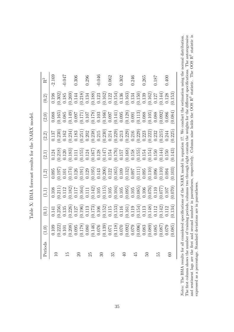
Tab

leX

:B

MA

fore

cast

resu

lts

for

the

NA

RX

model

.

Per

iods

(1,0

)(0

,1)

(1,1

)(1

,2)

(2,1

)(2

,2)

(2,0

)(0

,2)

R2

100.

109

0.14

10.

108

0.09

50.

124

0.13

70.

088

0.19

8-2

.169

(0.2

22)

(0.2

56)

(0.2

11)

(0.1

97)

(0.2

18)

(0.2

30)

(0.1

65)

(0.3

02)

150.

101

0.13

50.

112

0.10

10.

120

0.16

20.

085

0.18

5-0

.047

(0.2

08)

(0.2

26)

(0.1

82)

(0.1

74)

(0.1

83)

(0.2

34)

(0.1

49)

(0.2

69)

200.

095

0.12

70.

117

0.12

60.

111

0.18

30.

097

0.14

40.

306

(0.1

78)

(0.1

96)

(0.1

64)

(0.1

91)

(0.1

55)

(0.2

51)

(0.1

71)

(0.2

18)

250.

080

0.11

30.

111

0.12

90.

124

0.20

20.

107

0.13

40.

296

(0.1

46)

(0.1

73)

(0.1

42)

(0.1

95)

(0.1

67)

(0.2

38)

(0.1

78)

(0.1

88)

300.

076

0.10

60.

105

0.14

30.

128

0.21

50.

103

0.12

3-0

.046

(0.1

39)

(0.1

52)

(0.1

15)

(0.2

06)

(0.1

47)

(0.2

30)

(0.1

66)

(0.1

62)

350.

071

0.11

50.

105

0.12

20.

154

0.21

40.

097

0.12

20.

062

(0.1

18)

(0.1

53)

(0.1

04)

(0.1

65)

(0.1

76)

(0.2

29)

(0.1

41)

(0.1

54)

400.

070

0.11

60.

105

0.10

90.

157

0.21

30.

095

0.13

60.

302

(0.0

92)

(0.1

61)

(0.0

95)

(0.1

32)

(0.1

68)

(0.2

29)

(0.1

28)

(0.1

63)

450.

079

0.11

90.

105

0.09

70.

158

0.21

60.

091

0.13

40.

246

(0.0

96)

(0.1

54)

(0.0

85)

(0.1

11)

(0.1

55)

(0.2

29)

(0.1

13)

(0.1

50)

500.

083

0.11

30.

106

0.09

50.

154

0.22

30.

088

0.13

90.

265

(0.0

89)

(0.1

48)

(0.0

76)

(0.1

10)

(0.1

54)

(0.2

22)

(0.1

05)

(0.1

62)

550.

085

0.11

20.

110

0.09

60.

150

0.23

20.

088

0.12

70.

187

(0.0

87)

(0.1

42)

(0.0

77)

(0.1

10)

(0.1

44)

(0.2

15)

(0.0

92)

(0.1

44)

600.

079

0.11

20.

107

0.09

40.

150

0.24

40.

086

0.12

80.

400

(0.0

85)

(0.1

34)

(0.0

70)

(0.1

03)

(0.1

43)

(0.2

25)

(0.0

84)

(0.1

53)

Notes:

Th

eB

MA

resu

lts

for

all

con

sid

ered

spec

ifica

tion

sof

the

NA

RX

mod

elin

equ

ati

on

17.

We

con

du

ctth

ees

tim

ati

on

usi

ng

the

norm

al

dis

trib

uti

on

.T

he

firs

tco

lum

nsh

ows

the

nu

mb

erof

trai

nin

gp

erio

ds,

colu

mns

two

thro

ugh

eight

conta

inth

ew

eights

for

the

diff

eren

tsp

ecifi

cati

on

s.T

he

au

tore

gre

ssiv

ean

dse

nti

men

tla

gsar

eth

efi

rst

and

seco

nd

nu

mb

erin

pare

nth

eses

,re

spec

tive

ly.

Colu

mn

nin

eh

old

sth

eO

OS

R2

stati

stic

.T

he

OO

SR

2st

ati

stic

isex

pre

ssed

asa

per

centa

ge.

Sta

ndar

dd

evia

tion

sar

ein

pare

nth

eses

.

35

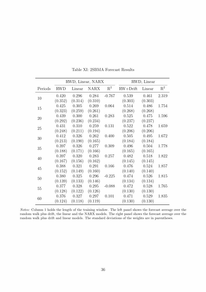
Table XI: 2SBMA Forecast Results

RWD, Linear, NARX RWD, Linear

Periods RWD Linear NARX R2 RW+Drift Linear R2

100.420 0.296 0.284 -0.767 0.539 0.461 2.319

(0.352) (0.314) (0.310) (0.303) (0.303)

150.425 0.305 0.269 0.064 0.514 0.486 1.754

(0.323) (0.259) (0.261) (0.268) (0.268)

200.439 0.300 0.261 0.283 0.525 0.475 1.596

(0.292) (0.236) (0.234) (0.237) (0.237)

250.431 0.310 0.259 0.131 0.522 0.478 1.659

(0.248) (0.211) (0.194) (0.206) (0.206)

300.412 0.326 0.262 0.400 0.505 0.495 1.672

(0.213) (0.190) (0.165) (0.184) (0.184)

350.397 0.326 0.277 0.309 0.496 0.504 1.778

(0.188) (0.171) (0.166) (0.165) (0.165)

400.397 0.320 0.283 0.257 0.482 0.518 1.822

(0.167) (0.156) (0.162) (0.145) (0.145)

450.388 0.321 0.291 0.166 0.476 0.524 1.857

(0.152) (0.149) (0.160) (0.140) (0.140)

500.380 0.325 0.296 -0.225 0.474 0.526 1.815

(0.139) (0.133) (0.146) (0.134) (0.134)

550.377 0.328 0.295 -0.088 0.472 0.528 1.765

(0.128) (0.122) (0.126) (0.130) (0.130)

600.376 0.327 0.297 0.101 0.471 0.529 1.835

(0.124) (0.118) (0.119) (0.130) (0.130)

Notes: Column 1 holds the length of the training window. The left panel shows the forecast average over therandom walk plus drift, the linear and the NARX models. The right panel shows the forecast average over therandom walk plus drift and linear models. The standard deviations of the weights are in parentheses.

36

Table XII: Peaks and troughs in Sentiment.

Peak Trough

195412 195707195808 196004196512 196608196707 197003197201 197212197504 197608197804 197902198001 198110198302 198406198703 198711199107 199207199601 199701199911 200011200306 200408200511 200806

Notes: The algorithm used to determine the turning points is described in sections V and appendix A.

Figure 1: The Sentiment Index vs Market Weighted returns

Notes: Shaded areas are bear markets defined by a 20 percent or drop over a two or month period.

37

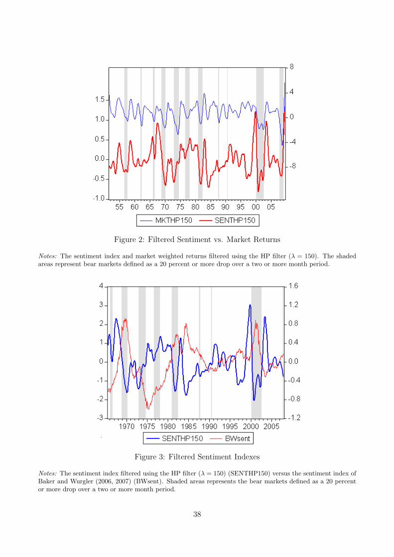
Figure 2: Filtered Sentiment vs. Market Returns

Notes: The sentiment index and market weighted returns filtered using the HP filter (λ = 150). The shadedareas represent bear markets defined as a 20 percent or more drop over a two or more month period.

Figure 3: Filtered Sentiment Indexes

Notes: The sentiment index filtered using the HP filter (λ = 150) (SENTHP150) versus the sentiment index ofBaker and Wurgler (2006, 2007) (BWsent). Shaded areas represents the bear markets defined as a 20 percentor more drop over a two or more month period.

38

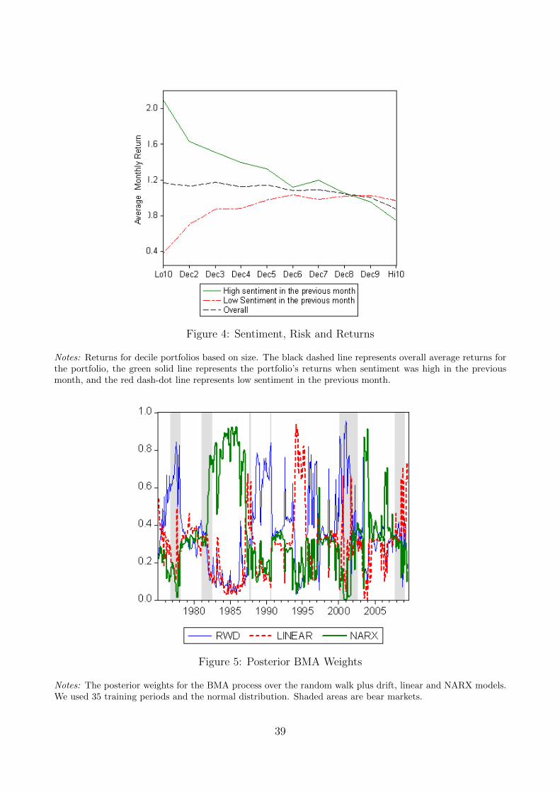
Figure 4: Sentiment, Risk and Returns

Notes: Returns for decile portfolios based on size. The black dashed line represents overall average returns forthe portfolio, the green solid line represents the portfolio’s returns when sentiment was high in the previousmonth, and the red dash-dot line represents low sentiment in the previous month.

Figure 5: Posterior BMA Weights

Notes: The posterior weights for the BMA process over the random walk plus drift, linear and NARX models.We used 35 training periods and the normal distribution. Shaded areas are bear markets.

39

Figure 6: Turning Points in Sentiment

Notes: The filtered sentiment index with λ = 150. Shaded areas represent peak to troughs in sentiment. Reddashed lines represent the beginning of bear markets. Green dash-dots lines represent the end of bear markets.

40

References

Abreu, Dilip, and Marcus K. Brunnermeier. 2003. “Bubbles and crashes.” Econometrica,71(1): 173–204.

Baker, Malcolm, and Jeffrey Wurgler. 2006. “Investor Sentiment and the Cross-Sectionof Stock Returns.” Journal of Finance, 61(4): 1645–1680.

Baker, Malcolm, and Jeffrey Wurgler. 2007. “Investor sentiment in the stock market.”Journal of Economic Perspectives, 21(2): 129–151.

Baker, Malcolm, Jeffrey Wurgler, and Yu Yuan. 2009. “Global, local, and contagiousinvestor sentiment.” Working Papers.

Barberis, Nicholas, Andrei Shleifer, and Robert Vishny. 1998. “A model of investorsentiment.” Journal of Financial Economics, 49(3): 307–343.

Barberis, Nicholas, Ming Huang, and Tano Santos. 2001. “Prospect Theory and AssetPrices.” Quarterly Journal of Economics, 116(1): 1–53.

Battalio, Robert, and Paul Schultz. 2006. “Options and the bubble.” Journal Of Finance,61(5): 2071.

Brown, Gregory W., and Michael T. Cliff. 2004. “Investor sentiment and the near-termstock market.” Journal of Empirical Finance, 11(1): 1–27.

Brown, Gregory W., and Michael T. Cliff. 2005. “Investor Sentiment and Asset Valua-tion*.” The Journal of Business, 78(2): 405–440.

Bry, Gerhard, and Charlotte Boschan. 1971. “Cyclical analysis of time series: selectedprocedures and computer programs.” NBER Books.

Campbell, John Y., and Samuel B. Thompson. 2007. “Predicting excess stock returnsout of sample: Can anything beat the historical average?” Review of Financial Studies.

Carter, CK, and R. Kohn. 1994. “On Gibbs sampling for state space models.” Biometrika,81(3): 541–553.

Chung, San-Lin, and Chung-Ying Yeh. 2009. “Investor Sentiment, Regimes and StockReturns.”

D’avolio, Gene. 2002. “The market for borrowing stock.” Journal of Financial Economics,66(2-3): 271–306.

De Long, J. Bradford, Andrei Shleifer, Lawrence H. Summers, and Robert J.Waldmann. 1990a. “Noise trader risk in financial markets.” The Journal of PoliticalEconomy, 98(4): 703–738.

De Long, J. Bradford, Andrei Shleifer, Lawrence H. Summers, and Robert J.Waldmann. 1990b. “Positive feedback investment strategies and destabilizing rationalspeculation.” The Journal of Finance, 45(2): 379–395.

41

Fama, Eugene F., and Kenneth R. French. 1993. “Common risk factors in the returnson stocks and bonds* 1.” Journal of financial economics, 33(1): 3–56.

Foresee, F. Dan, and Martin T. Hagan. 1997. “Gauss-Newton approximation to Bayesianlearning.” Vol. 3, 1930–1935, Piscataway: IEEE.

Gervais, Simon, and Terrance Odean. 2001. “Learning to be overconfident.” Review ofFinancial Studies, 14(1): 1.

Glushkov, Denys. 2006. “Sentiment beta.” Working Paper.

Goyal, Amit, and Ivo Welch. 2008. “A comprehensive look at the empirical performanceof equity premium prediction.” Review of Financial Studies, 21(4): 1455–1508.

Grinblatt, Mark, and Bing Han. 2005. “Prospect theory, mental accounting, and momen-tum.” Journal of Financial Economics, 78(2): 311–339.

Hoeting, Jennifer A., David Madigan, Adrian E. Raftery, and Chris T. Volinsky.1999. “Bayesian model averaging: A tutorial.” Statistical science, 14(4): 382–401.

Kim, Chang-Jin, and Charles R. Nelson. 1998. “Business cycle turning points, a newcoincident index, and tests of duration dependence based on a dynamic factor model withregime switching.” Review of Economics and Statistics, 80(2): 188–201.

Kim, Chang-Jin, and Charles R. Nelson. 1999. State-space models with regime switching.MIT press Cambridge, MA.

Lee, Charles M.C., Andrei Shleifer, and Richard H. Thaler. 1991. “Investor sentimentand the closed-end fund puzzle.” The Journal of Finance, 46(1): 75–109.

Lemmon, Michael, and Evegenia Portniaguina. 2006. “Consumer confidence and assetprices: Some empirical evidence.” Review of Financial Studies, 19(4): 1499.

Lutz, Chandler J. 2010. “Stock Market Forecasting Using Agent Sentiment.” Working Pa-pers.

MacKay, David J.C. 1992. “A practical Bayesian framework for backpropagation networks.”Neural computation, 4(3): 448–472.

Pesaran, M. Hashem, and Allan Timmermann. 1995. “Predictability of stock returns:Robustness and economic significance.” The Journal of Finance, 50(4): 1201–1228.

Qiu, Lily X., and Ivo Welch. 2004. “Investor sentiment measures.” Working Paper.

Raftery, Adiran E. 1995. “Bayesian model selection in social research.” Sociological method-ology, 25: 111–163.

Raftery, Adrian E., Tilmann Gneiting, Fadoua Balabdaoui, and Michael Po-lakowski. 2005. “Using Bayesian model averaging to calibrate forecast ensembles.”Monthly Weather Review, 133(5): 1155–1174.

42

Shiller, Robert J. 2006. Irrational exuberance. Broadway Business.

Stambaugh, Robert F. 1999. “Predictive Regressions.” National Bureau of Economic Re-search, Inc NBER Technical Working Papers 0240.

Timmermann, Allan. 2008. “Elusive return predictability.” International Journal of Fore-casting, 24(1): 1–18.

Wasserman, Phillip D. 1993. Advanced methods in neural computing. John Wiley & Sons,Inc. New York, NY, USA.

Whaley, Robert E. 2000. “The investor fear gauge.” The Journal of Portfolio Management,26(3): 12–17.

43