AFFINE PROCESSES FOR DYNAMIC MORTALITY AND

ACTUARIAL VALUATIONS

ENRICO BIFFIS?

Istituto di Metodi Quantitativi, Università Bocconi

Abstract. We address the risk analysis and market valuation of lifeinsurance contracts in a jump-diffusion setup. We exploit the analyti-cal tractability of affine processes to deal simultaneously with financialand demographic risks affecting a wide range of insurance covers. Wethen focus on mortality at pensionable ages and show how the risk oflongevity can be taken into account. A parallel with the pricing ofcertain credit risky securities is drawn, in order to employ importantresults derived in that field.

Keywords: affine jump-diffusion, stochastic mortality, doubly stochastic pro-cesses, longevity risk, fair value.

JEL: G13, G22, J11, M40.Subj. Class.: IM40, IB10, IB13.

? Istituto di Metodi Quantitativi, Università Bocconi - Viale Isonzo 25, 20135 Milano, Italy.Tel.: +390258365556. Fax: +390258365630. E-mail: ebiffis@unibocconi.it.

First version: 1st June 2004. This version: 4th October 2004. This paper revises and extendsBiffis (2003). Earlier versions have been presented at the 8th IME Congress in Lyon, at the 6th

Spanish-Italian Meeting on Financial Mathematics in Trieste, at the University of Parma andat the ETH in Zürich. I would like to thank the participants in those conferences and seminarsfor helpful comments and suggestions. All errors are mine. I acknowledge financial supportfrom the Italian MIUR.

1. Introduction

Actuarial valuations involve the consideration of at least two types of uncer-tainty in life insurance: uncertainty related to financial factors (financial risk)and uncertainty related to the random residual lifetime of insureds (mortalityrisk). Mortality is traditionally modeled deterministically, either assuming suit-ably parameterized analytical models, either adopting adjusted/projected mor-tality tables. Recent mortality trends have proved particularly challenging forthe pricing and reserving related to contracts providing long-term living benefits(e.g. Olivieri, 2001; Pitacco, 2003a) and have called for more effective approaches.

Valuation models cannot fully capture the dynamics of insurance business un-less both risks are modeled adequately. In this regard, a new impulse to a soundand articulated valuation of insurance contracts has been recently prompted bythe release of IASB (2001, 2004) by the International Accounting Standards Board(IASB) and by the support shown by several institutions to the principles thereproposed. The IASB’s proposals acknowledge the need to deal explicitly withall sources of risk, including non-financial risks, both diversifiable (e.g. mortal-ity random fluctuations around expected levels) and non fully diversifiable (e.g.systematic departures of mortality from expected levels), and advocate the ac-counting of insurance liabilities at market value. Specifically, the IASB definesfair value of a book of insurance liabilities its exchange price in a (hypothetical)secondary market transaction. Since a deep wholesale market for such liabilitiesdoes not exist, exchange prices are not easily observable. However, ‘no-arbitragetype’ arguments imply that the fair value of an insurance liability should notbe too different from the market value of a portfolio of traded assets matchingbroadly the liability cashflows. Indeed, the IASB favours the use of an expecteddiscounted cashflow approach consistent with risk-neutral valuation.

Any valuation model confronts actuaries and insurance practitioners with atrade-off between complexity and computational tractability of pricing and esti-mation. In this respect, affine jump-diffusions are stochastic processes that haveshown themselves to be useful in developing tractable and flexible dynamic assetpricing models. They have been extensively used in modeling the term structureof interest rates (see Dai and Singleton, 2000, and references therein), stochasticvolatility for currency and equity prices (e.g. Bakshi, Cao and Chen, 1997) andthe risk of default of corporate bonds and other credit-risky securities (e.g. Lando,1998).

In this work, we model asset prices and mortality dynamics by using affinejump-diffusions. In this way, we are able to fully exploit the analytical tractabilityof affine processes in the context of both financial and mortality risk. Moreover,by drawing a parallel between insurance contracts and certain credit-sensitivesecurities (first suggested in Artzner and Delbaen, 1995, and recently used byMilevsky and Promislow, 2001; see also Dahl, 2004) we exploit some results ofthe so called intensity-based approach to credit risk modelling to derive closed-form expressions for the pricing and reserving of the most common life insurancecontracts. We also outline a link with a popular actuarial valuation methodology,the Embedded Value Method, and provide valuation formulae whose implemen-tation is straightforward and consistent with the framework proposed in IASB(2001, 2004).

2

The paper is organized as follows. In Sec. 2, we draw a parallel betweeninsurance contracts and some defaultable securities. In Sec. 3, we sketch themain characteristics of affine processes and present the most useful results forfinancial applications. Sec. 4 describes the financial and insurance market ofconcern, presenting the framework to be employed for risk-analysis and marketvaluations or just for stand-alone mortality modeling. Sec. 5 offers valuationexpressions for a large class of (possibly unit-linked or indexed) life insurancecontracts where mortality, the term structure of interest rates and asset pricesare all modeled stochastically. In Sec. 6, we show how affine jump-diffusions canbe used to describe the dynamics of human mortality and to deal with the socalled ‘longevity risk’, providing in turn some numerical examples. Sec. 7 offersconcluding remarks. Additional results and details are provided in the Appendix.

2. Insurance Contracts and Credit-risky Securities

There are two main approaches to valuing credit-sensitive securities (see Jean-blanc and Rutkowski, 2000, for a detailed overview): the structural approach,which aims at determining the default event by modeling the dynamics of thefirm’s assets, and the reduced-form approach, under which the default time ismodeled as a stopping time that occurs as a total surprise. The latter approachrelies on the exogenous specification of the conditional probability of default,given that default has not yet occurred. This is usually done by modeling theintensity of default, which is allowed to depend on observables or unobservablesvariables. Among the first papers to advocate the use of such approach wasArtzner and Delbaen (1995), where a parallel with the pricing of annuities wasdrawn. It seems thus logical to go back to that insight and employ it for actuarialpurposes.

A key result of intensity-based modeling is that the pricing of credit-sensitivesecurities can be carried out in the same way as for risk-free financial instruments,provided discounting (under a ‘risk-neutral’ probability) is performed by usingan adjusted (or fictitious) short rate accounting for the probability and timingof default. This means that all of the arsenal of term-structure models can beapplied by suitably parameterizing the adjusted short rate instead of the risk-freerate. In particular, let R be the adjusted short rate process and Bd(0, T ) theprice of a defaultable zero coupon bond with maturity T and face value 1. Then,from results in (e.g.) Lando (1998), under technical conditions, we have:

Bd(0, T ) = E[e−

∫T

0 Rsds]

+

∫ T

0wsqsds, (1)

where the first term on the right hand side is the current price of a claim payingone unit at maturity in case of no default, zero otherwise, while the second terminvolves ws, representing the proceeds from default (recovery) if it occurs at times, and qs, the price density of a claim paying one unit if default occurs in (s, s+ds).See Sec. 5.1 for a detailed analysis of the result.

The form of expression (1) is remarkably useful from the point of view of in-terpretation and extremely appealing from that of computation, as will be shownin Sec. 3, where the analytical tractability of the affine setting is described. If weinterpret default as the event ‘insured’s death’ and the intensity of default as theintensity of mortality, we can see that expression (1) covers quite a large class of

3

traditional insurance contracts. For example, endowments of arbitrary maturity,as well as of different benefit amounts, are encompassed by (1). Moreover, annu-ities are covered by combinations1 of terms like the expectation appearing in (1)for different maturities (annuity payment dates), while assurances are covered bythe only second term in (1). Of course, the interpretation of the default eventis reverted: for example, an annuity stops being paid because an insured (thereceiver of the benefits) dies, while coupons from a bond cease to be paid becausethe issuer (the one who pays coupons and principal) has defaulted. We point outthat we will not treat the issue of a possible default by the insurer.

Viewing an endowment as a defaultable zero-coupon bond, or an annuity as adefaultable consol (with zero recovery) yields several advantages. For example,it is easier to take into account the joint effect of mortality and financial risks,as will be shown in Sec. 5. This is particularly important for those productsfeaturing embedded options depending on both sources of risk (see Biffis andMillossovich, 2004, for an application to guaranteed annuity options). Further-more, adjusted discount rates, which are crucial to any profit testing or embeddedvalue computation, can be given a sound theoretical background for the mortal-ity risk component. The framework proposed can therefore be beneficial in manyrespects, from pricing and reserving to preparing financial statements consistentwith the IASB’s accounting standards.

3. Affine Processes

Affine processes are a class of Markov processes with conditional characteristicfunction of the exponential affine form. A thorough treatment of such processesis provided in Duffie, Filipovič and Schachermayer (2003) and Filipovič (2001).In this section, we adopt the narrower but more usual (in financial applications)perspective based on the definition of affine processes in terms of strong solutionsto specific stochastic differential equations (SDEs) in a given filtered probabilityspace (e.g. Duffie and Kan, 1996; Duffie, Pan and Singleton, 2000).

We fix a probability space (Ω,F , P) and a filtration F = (Ft)t≥0 satisfying theusual conditions2 and representing the information available up to time t. AnRn-valued affine jump-diffusion X is an F-Markov process specified as the strongsolution to the following SDE:

dXt = δ(t,Xt)dt + σ(t,Xt)dWt + dJt, (2)

where W is an F-standard Brownian motion in Rn and J is a pure-jump processin Rn with jump-arrival intensity κ(t,Xt) : t ≥ 0 and time-dependent jumpdistribution νt on Rn. We require the drift δ, the instantaneous covariance matrixσσT and the jump-arrival intensity κ to have all affine dependence on X, asexplained in App. A.

An important result holds for analytical approaches based on the affine struc-ture described. For any c ∈ C and a, b ∈ Cn, for given T ≥ t and affine function Λ

1We can always see an annuity as a set of pure endowments, just as coupon bearing bondscan be stripped.

2That is, (P,F)-completeness and right continuity: see Protter (2004, p. 3). We refer thereader to the same source for background and terminology. In what follows, all filtrations areassumed to satisfy the usual conditions.

4

defined by Λ(t, x) = λ0(t)+λ1(t) ·x (for some bounded continuous R×Rn-valuedfunction λ

.= (λ0, λ1)), under technical conditions the following expression holds:

E[e−

∫T

tΛ(s,Xs)ds ea·XT (b · XT + c)

∣∣∣Ft

]= eα(t)+β(t)·Xt

[α(t) + β(t) · Xt

], (3)

where α(·) .= α(·; a, T ), β(·) .

= β(·; a, T ), α(·) .= α(·; a, b, c, T ) and β(·) .

=

β(·; a, b, T ) are functions solving uniquely a set of ordinary differential equations(ODEs) specified in App. A, with boundary conditions α(T ) = 0, β(T ) = a,

α(T ) = c and β(T ) = b. One can immediately see the importance of these re-sults in deriving analytical solutions for a variety of financial applications. Forexample, we will be interested in the following:

First, the entire class of affine term structure models is obtained as a specialcase of (3) when we take expectation under a risk-neutral probability measureand set rs

.= Λ(s,Xs) (rs being the short rate process), a, b = 0 and c = 1. This

class includes: the model proposed by Vasicek (1977), where X is a GaussianOhrnstein-Uhlenbeck process; the CIR model (Cox, Ingersoll and Ross, 1985),where X is a Feller difffusion; the general multivariate models introduced byDuffie and Kan (1996) and several other extensions (see Dai and Singleton, 2000,and references therein).

Second, expression (3) can be used in a similar fashion for risk-neutral valua-tion, when asset prices have an exponential affine form, as is assumed in manyfinancial applications (see Sec. 4.1 and references therein). More generally, theexpected discounted cash flow approach (with discount rate Λ(s,Xs)) can be im-plemented for all discounted cash flows whose form is encompassed by the termunder expectation in (3).

Third, the transform (3) can be used in credit risk modeling, when the timeof default of a financial counter-party is modeled as the first jump time of adoubly stochastic process N driven by an affine process X. In such framework,the intensity of N has the form Λ(s,Xs−) : s ≥ 0 and (3) can be used, forexample, with a, b = 0 and c = 1 to compute the probability of no default by T ,conditional on Xt and survival to t (see Sec. 4.2).

The analytical tractability of affine processes is essentially linked to the ODEsassociated with the transform (3). They are generalized Riccati equations thatcan be solved by using standard numerical methods. For some specifications ofthe parameters δ, σ, κ and ν, explicit solutions are available. They are derived,for example, in the simple case of the Vasicek and CIR model without jumps.When including jumps, explicit solutions may be available when the jump-arrivalprocess is Poisson, depending on the specification of ν. In the Vasicek case, thechoice of the jump distribution can be very general. In the CIR case, the choiceis more restricted, due to the non-negativity requirement for X: closed-formsolutions are available with degenerate (fixed jump size), uniform, exponentialand binomial jump-size distributions (see Duffie and Kan, 1996, for example).

4. Modeling Framework

In this section we introduce the modeling framework. We shall first introduce thefinancial market (Sec. 4.1) and the mortality model (Sec. 4.2) separately, and thensuccessively combine them to describe the insurance market model (Sec. 4.3).

5

4.1. Financial Market. We fix a filtered probability space (Ω,F , F, P). We take

as given an adapted short-rate process r (such that∫ t

0 |rs|ds < ∞ for all t ≥ 0)representing the continuously compounded rate of interest on riskless securities.This can be formalized by assuming the presence in the market of a money-market

account Bt = exp(∫ t

0 rsds) representing the amount of money available at timet from investing one unit at time 0 in risk-free deposits and ‘rolling over’ theproceeds until t.

We assume that at least a security is traded continuously in the market, with anonnegative semimartingale S representing its ex-dividend price. In the absenceof arbitrage, an equivalent martingale measure Q exists, under which which thegain (from holding the security) process is a martingale after deflation by themoney-market account. Specifically, let D be a process of locally integrable vari-ation representing the security’s cumulated dividend. Then, the discounted gainprocess is given by (B−1

t St +∫ t

0 B−1s dDs) and the following convenient formula

applies:

St = EQ

[e−

∫T

trsdsST +

∫ T

t

e−∫

u

trsdsdDu

∣∣∣Ft

]. (4)

In what follows, we will assume that the price of any security is zero after agiven time t > 0 if the security pays no dividends thereafter. If the security hasdividend yield process ζ, i.e. the instantaneous yield from holding the security is

ζtStdt, then Dt =∫ t

0 ζuSudu and the martingale property implies that S has driftr − ζ under Q, justifying the appellation ‘risk-neutral’ for this measure. Whenconsidering several securities, including zero-coupon bonds, the no-arbitrage re-striction imposed by (4) must apply simultaneously to each security price process.From now on, we assume that the dynamics of all security processes are specifiedunder Q unless otherwise stated. We refer the reader to Duffie (2001) for moredetails on no-arbitrage pricing.

We then postulate that all security prices are driven by an affine process Xin Rk. Specifically, we assume that r is expressed as rt

.= R(t,Xt), where Xt

satisfies (2) and the conditions there given and R is an affine function defined byR(t, x) = ρ0(t)+ρ1(t) ·x, with ρ

.= (ρ0, ρ1) an R×Rk-valued bounded continuous

function on [0,∞). An immediate consequence (use (4) and (3)) is that for fixedT ≥ t > 0, the time t-price B(t, T ) of a zero coupon bond with maturity T (i.e.a security paying a single dividend equal to 1 at time T ), has exponential affineform.

When considering risky securities, we take their log-price to be an affine pro-cess. Specifically, let us consider the price process S of a risky security havingan affine dividend-yield process ζ(t,Xt) = q0(t) + q1(t) · Xt, with q

.= (q0, q1) an

R×Rk-valued bounded continuous function on [0,∞). Without loss of generality(see Duffie, Pan and Singleton, 2000, Sec. 3.1) we can set log(S) equal to (say)Xi, the i-th component of X. In the absence of arbitrage, the dynamics of S mustobey the restrictions implied by (4) and outlined in App. B. Similar restrictionsmust be imposed for any additional risky security of this type considered in themarket.

The setup outlined is fairly general: security price processes featuring stochasticvolatility or discontinuous dynamics are naturally included. For example, thefinancial market models used by Bakshi, Cao and Chen (1997), Bakshi and Madan

6

(2000), Bates (2000), Heston (1993) and Scott (1997) are all encompassed by theframework described. See also Eraker, Johannes and Pohlson (2003).

4.2. Mortality Model. We fix a filtered probability space (Ω,F , F, P) and focuson an insured aged x at time 0. We model his/her random residual lifetime as anF-stopping time τx admitting a random intensity µx. Specifically, we regard τx asthe first jump-time of a nonexplosive F-counting process N recording at each timet ≥ 0 whether the individual has died (Nt 6= 0) or not (Nt = 0). The stoppingtime τx is said to admit an intensity µx if N does, i.e. if µx is a nonnegative

predictable process such that∫ t

0 µx(s)ds < ∞ for all t ≥ 0 and such that the

compensated process M = Nt −∫ t

0 µx(s)ds : t ≥ 0 is a local F-martingale.

If, in addition, E[∫ t

0 µx(s)ds] < ∞ for all t ≥ 0, then M is an F-martingale.

(Alternatively, we could look at the single jump process Nt = Iτx≤t and take

as intensity of N a predictable process µx that is equal to µx up to time τx,

the intensity of N loosing meaning thereafter.) We refer the reader to Brémaud(1981), Jeanblanc and Rutkowski (2000) and Duffie (2001) for details.

The idea behind a stochastic intensity is that, at any time t ≥ 0 and stateω ∈ Ω such that τx(ω) > t, we have:

P(τx ≤ t + ∆|Ft)(ω) ∼= µx(t, ω)∆ (5)

for small ∆ > 0. This is the stochastic analogue of the expression for the ‘instan-taneous death probability’:

∆qx+t∼= m(x + t)∆, (6)

which is familiar to actuaries and usually emerges when defining the deterministicintensity m itself (see Bowers, Gerber, Hickman, Jones and Nesbitt, 1997, foractuarial background and notation). Actually, expressions (5) and (6) coincidewhen F is the smallest filtration making τx a stopping time, i.e. when Ft =σ(Iτx≤s; 0 ≤ s ≤ t) for all t ≥ 0. We remark, however, that our setup is bothstochastic and dynamic, since the distinguishing features of µt(ω) are: the ‘stateof the world’ ω ∈ Ω determining the particular trajectory of µ; the date t ≥ 0,i.e. the continuous-time counterpart of the calendar year of reference used inlongitudinal tables. Thus, we are naturally adopting a diagonal, or cohort-based,approach (see Pitacco, 2003b).

From an actuarial viewpoint, we may see expression (5) as emphasizing thestochastic variation of the intensity over time, as new information about the in-sureds’mortality becomes available. This corresponds to a change of demographicbasis, represented by the choice/availability of a new intensity (or of a new lifetable from which the intensity is derived) at each time t. We do not specify whatkind of basis, realistic or prudential for example, consistently with the choice ofremaining very general in this section about the probability measure P underwhich expectations are taken (see Sec. 5.4 for details).

If the insured is representative of a group of policyholders (e.g. same age andhealth status), then the results obtained in the sequel extend to all individualsbelonging to the homogeneous population, provided the individual random resid-ual lifetimes can be thought as independent and identically distributed. Keep-ing this in mind, from now on we drop reference to the age x and set τ = τx,µt(ω) = µx(t, ω) and m(x + t) = m(t).

7

To improve analytical tractability, we further assume that N is a doubly sto-

chastic (or Cox) process driven by a subfiltration G of F, with G-predictable in-tensity µ. Intuitively, this means that, conditionally on any particular trajectoryt 7→ µt(ω) of µ, the counting process N becomes Poisson-inhomogeneous withparameter

∫ ·0 µs(ω)ds. Formally, we have that for all T ≥ t ≥ 0 and nonnegative

integer k, the following holds:

P(NT − Nt = k|Ft ∨ GT ) =

(∫ T

tµsds

)k

k!e−

∫T

tµsds (7)

The idea behind the specification of G is that it provides enough informationabout the evolution of the intensity of mortality, i.e. about the likelihood ofdeath happening, but not enough information about the actual occurrence ofdeath. Such information is carried by the larger filtration F, with respect towhich τ is a stopping time.

The application of the law of iterated expectations and the use of (7) withk = 0 yield that the ‘probability of survival’ up to time T ≥ t, on the set τ > t,is given by:

P(τ > T |Ft) = E[e−

∫T

tµsds

∣∣∣Ft

](8)

This can be compared with its deterministic analogue, which, in usual actuarialnotation, reads:

T−tpx+t = e−∫

T

tm(s)ds, (9)

where T−tpx+t indicates the probability of surviving T − t years for an individualaged x + t years at time t.

Furthermore, under technical conditions reviewed in Grandell (1976, pp. 105-107), the Ft-conditional density ft(·) of τ is given, on the set τ > t, by theexpression:

ft(s) =∂

∂sP(τ ≤ s|Ft) = E

[µs e−

∫s

tµudu

∣∣∣Ft

](10)

It is clear that both (8) and (10) are particular cases covered by the transform(3), so that working in an affine framework would be very convenient from thecomputational point of view. We therefore take an Rd-valued affine jump-diffusionY and its natural filtration GY = (GY

t )t≥0, with GYt = σ(Ys : 0 ≤ s ≤ t), as

subfiltration of F. We then consider µs.= M(s, Ys−), for some function M(t, y) =

η0(t) + η1(t) · y, with η.= (η0, η1) an R×Rd-valued bounded continuous function

such that µ is nonnegative. We take the left limits of Y , because the state variablesprocess needs not be predictable. That makes no difference for expressions (8)and (10), however, since the pure jump process of (2) has at most a countable

number of jumps and thus∫ T

tM(s, Ys−)ds =

∫ T

tM(s, Ys)ds a.s. for all T ≥ t.

In Sec. 6 we show how suitable choices of η and Y lead to an effective descriptionof the dynamics of human mortality.

4.3. Combined Model. We parallel one of the standard setups employed inthe valuation of credit-risky securities. We consider a filtered probability space(Ω,F , F, P) large enough to support a process X in Rk, representing the evolu-tion of financial variables, and a process Y in Rd, representing the evolution ofmortality. Moreover, we focus on a representative insured aged x at time 0, withrandom residual lifetime described as in Sec. 4.2 by an F-stopping time τ .

8

The filtration F = (Ft)t≥0 represents the flow of information available as timegoes by: this includes knowledge of the evolution of all state variables up to eachtime t and of whether the policyholder has died by then. Formally, we write:

Ft = Gt ∨Ht

where Gt ∨Ht is the σ-algebra generated by Gt ∪Ht, with

Gt = σ(Zs : 0 ≤ s ≤ t)

Ht = σ(Iτ≤s : 0 ≤ s ≤ t),

and where Z = (X,Y ) is the joint state variables process in Rk+d. Thus, we haveF = G∨H, with G = GX ∨GY and with H = (Ht)t≥0 being the smallest filtrationwith respect to which τ is a stopping time.

In the absence of arbitrage, an equivalent martingale measure Q exists, underwhich all financial security prices are martingales after deflation by the moneymarket account (see Sec. 4.1). Under Q, we assume that X and Y are independentand, on the lines of Sec. 4.2, that τ is doubly stochastic driven by GY ⊂ F. Itis worth emphasizing that the latter property does not need to preserve undermeasure changes and that any such changes determine a modification in theintensity process µ. However, an intensity is guaranteed to exist under Q if τadmits an intensity under, say, the ‘physical’ measure P (see Artzner and Delbaen,1995).

5. Valuation of Life Insurance Contracts

In this section, we start with the valuation results derived for the basic insurancecontracts paying a single (random) benefit upon survival at a given date or upondeath within a certain period of time (Sec. 5.1). These results are extended inSec. 5.2 to several types of insurance contracts, including traditional, unit-linkedand indexed policies. We adopt a ‘no-arbitrage type’ valuation framework, consis-tent with the methodology proposed by IASB (2001, 2004) for the measurement ofinsurance liabilities at market value and refer to the prices obtained as fair values.The caveats under which such approach can be applied are discussed in Sec. 5.3,while Sec. 5.4 discusses the meaning of the risk-neutral probability measure Q in-troduced in the previous section. More generally, the expressions provided in thesequel can be looked to in terms of expected discounted cash-flow approach (seeSec. 3): the process r can be replaced by a suitable discount rate, the measureQ by a measure other than risk-neutral; the results obtained can then be usedfor risk-management purposes (e.g. sensitivity analysis, stress testing, etc.). Inany case, all expectations appearing in the sequel are to be understood as takenunder a given probability measure Q.

5.1. Building-blocks. We provide the fair values of two basic payoffs involvedby standard insurance contracts. These are benefits, of amount possibly linkedto other security prices, contingent on survival or death over a given time period.The modeling framework is as described in Sec. 4.3, but for the moment no explicitreference is made to the affine dynamics of the process Z = (X,Y ) in Rk+d. Weonly require the short rate process r and the intensity of mortality µ to satisfythe technical conditions stated in Sec. 4.1 and Sec. 4.2.

9

Proposition 5.1 (Survival Benefit). Let C be a bounded G-adapted process.

Then, the time-t fair value SBt(CT ;T ) of the time-T survival benefit of amount

CT , with 0 ≤ t ≤ T , is given by:

SBt(CT ;T ) = E[e−

∫T

trsdsIτ>TCT

∣∣∣Ft

]

= 1τ>tE[e−

∫T

t(rs+µs)dsCT

∣∣∣Gt

] (11)

In particular, if C is GX-adapted, the following holds:

SBt(CT ;T ) = 1τ>tE[e−

∫T

trsdsCT

∣∣∣GXt

]E[e−

∫T

tµsds

∣∣∣GYt

](12)

Proof. We can use the law of iterated expectations, the fact that r and C areG-adapted, to write:

SBt(CT ;T ) = E[e−

∫T

trsdsCT E

[Iτ>T

∣∣∣Ft ∨ GT

] ∣∣∣Ft

]

From this, we note that SBt(CT ;T ) is zero on the set τ ≤ t. Focusing on theset τ > t, we exploit the doubly stochastic property, obtaining:

SB t(CT ;T ) = 1τ>tE[e−

∫T

t(rs+µs)dsCT

∣∣∣Ft

].

The conditioning on Ft can be reduced to that on Gt, as shown in App. C.Expression (12) is finally obtained by exploiting the independence of the filtrationsGX and GY . We use the following fact: given two independent filtrations F1 =(F1

t )t≥0

and F2 = (F2t )

t≥0, for any bounded random variables V 1 and V 2 that are

F1∞- and F2

∞-measurable, one has E[V 1V 2|F1t ∨F2

t ] = E[V 1|F1t ]E[V 2|F2

t ] for allt ≥ 0.

We note that the results in Prop. 5.1 hold also for survival benefits whosevalue is known at an earlier date u, with t < u ≤ T . This is useful when valuingcontracts providing benefits linked to the level attained by some reference fund atdiscrete times. Similarly, this helps in valuing some forms of with-profit businessshowing a ‘lagging’ mechanism between the indexation date and the payment ofthe benefits.

Proposition 5.2 (Death Benefit). Let C be a bounded G-predictable process.

Then, the time-t fair value DBt(Cτ ;T ) of the death benefit of amount Cτ , payable

in case the insured dies before time T , with 0 ≤ t ≤ T , is given by:

DBt(Cτ ;T ) = E[e−

∫τ

trsdsCτ It<τ≤T

∣∣∣Ft

]

= Iτ>t

∫ T

t

E[e−

∫u

t(rs+µs)dsµuCu

∣∣∣Gt

]du

(13)

In particular, if C is GX-predictable, the following holds:

DBt(Cτ ;T ) = Iτ>t

∫ T

t

E[e−

∫u

trsdsCu

∣∣∣GXt

]E[e−

∫u

tµsdsµu

∣∣∣GYt

]du (14)

Proof. We first note that the process (Cu exp(−∫ u

trsds))u≥t is predictable with

respect to (Gu)u≥t. Since the predictable σ-algebra on Ω × [t, T ] is generatedby the left-continuous adapted processes on [t, T ] (e.g. Kallenberg, 2002, Lemma25.1(iii)), any predictable process on [t, T ] can be generated by the elementary

10

predictable process (Zu)t≤u≤T , where Zu.= ZtIu=t + ZhIh<u≤k with Zh ∈ Gh

for each h and for all t ≤ h < k ≤ T . For u = τ , We can thus write:

E[ZhIh<τ≤k

∣∣∣Ft

]= E

[Zh

(Iτ>h − Iτ>k

) ∣∣∣Ft

]

= E[ZhE

[Iτ>h − Iτ>k

∣∣Ft ∨ Gk

] ∣∣∣Ft

]

= Iτ>tE[Zh

(e−

∫h

0 µsds − e−∫

k

0 µsds) ∣∣∣Ft

]

= Iτ>tE

[Zh

∫ k

h

e−∫

u

0 µsdsµudu∣∣∣Ft

]

= Iτ>tE

[∫ T

t

e−∫

u

0µsdsµuZudu

∣∣∣Ft

],

where we have used the law of iterated expectations in the second line and the dou-bly stochastic property in the third. The result then follows by a monotone classargument, paired by use of the (conditional) Fubini theorem and by reduction ofthe conditioning to Gt (see App. C). Finally, the factorization (14) is obtained byemploying the same argument used in the proof of (12) in Prop. 5.1.

Prop. 5.1 and Prop. 5.2 formalize what was outlined in Sec. 2. The risk-neutral valuation formula (4) extends naturally to securities providing benefitscontingent on mortality, provided they are treated as fictitious securities payingout dividends at a rate of µC, under a fictitious (or risk-adjusted) short rateprocess r + µ. We point out that the whole filtration G (and not only GX)may carry information concerning the random benefits, enabling to deal withdeferred insurance contracts and with benefits linked to mortality experience aswell. This is the case, for example, of insurance contracts providing returnslinked in some way to the demographic profit of the insurer. Even when thefactorizations (12) and (14) cannot be used, expressions (11) and (13) have agreat analytical tractability in the affine setting, as shown, for example, in Biffisand Millossovich (2004) with reference to insurance contracts embedding optionsto convert survival benefits into annuities.

5.2. Life Insurance Contracts. We can cover quite a large class of insurancecontracts by suitably combining the building blocks described in Sec. 5.1. First,we note that the valuation of traditional, unit-linked and indexed contracts canbe performed with the same instruments. Indeed, the only difference resides inwhether the benefit process C mentioned in Prop. 5.1 and Prop. 5.2 is determinis-tic or random. In the former case, we can value traditional insurance contracts; inthe latter, unit-linked or indexed contracts, depending on whether the evolutionof C represents the value of a reference fund or an index. With this regard, weunderline that (transformations of) suitable traded security prices may be takenas a proxy for inflation or other indexes. An example is provided below withreference to a floating-rate annuity.

We now present an overview of the contracts encompassed by our framework,always referring to contracts taken out at time 0 by a policyholder then aged xyears. We try to use standard actuarial notation whenever possible.

Assurances: the fair value T Ax(C) of a T -years term assurance guaranteeinga benefit C satisfying the assumptions of Prop. 5.2 and payable in case of death

11

in the period (0, T ], is simply given by:

T Ax(C) = DB0(Cτ ;T ).

For a whole life assurance, we just need to extend the maturity to the maximumage x∗ (alternatively, to +∞, provided integrability conditions hold), the one towhich no one is assumed to survive:

Ax(C) = DB0(Cτ ;x∗ − x).

Endowments: the fair value Ax:T e(C′, C ′′) of a T -years generic endowment

involving a survival benefit C ′ and a death benefit C ′′, satisying the conditionsof Prop. 5.1 and Prop. 5.2, respectively, is given by the combination of (11) and(13):

Ax:T e(C′, C ′′) = SB0(C

′T ;T ) + DB0(C

′′τ ;T )

The expression includes pure (C ′′ = 0) and standard (C ′ = C ′′) endowments,as well as more complicated structures. For example, the fair value of a double

endowment (involving a whole life assurance and a pure endowment) is simplyobtained by summing SB0(C

′T ;T ) and DB0(C

′′τ ;x∗ − x), possibly with C ′ = C ′′.

Annuities: the fair value of an annuity can be obtained by combining pureendowments. As an example, consider an annuity paying continuously an in-stantaneous benefit rate C over the policyholder’s life time, with the process Csatisfying the conditions of Prop. 5.1. Its fair value ax(C) is given by:

ax(C) =

∫ x∗−x

0SB0(Cs; s)ds (15)

Expression (15) can be used to value premium cash flows as well. For example,a stream of continuous premium payments at a rate of π over the period [0, T )(with T ≤ x∗ − x), where the process π satisfies the conditions of Prop. 5.1, has

fair value:∫ T

0 SB0(πs; s)ds.

The discrete versions of the insurance contracts considered is straightforward.For example, consider an immediate annuity paying a benefit C (satisfying theconditions of Prop. 5.1) at the beginning of times 0, 1, 2, . . . in case of the insured’ssurvival at each policy date. The analogue of (15) is given by

ax(C) =x∗−x−1∑

h=0

SB0(Ch;h) (16)

We finally present an example of indexed contract. Let us consider a t-yearsdeferred annuity involving a continuous payment of an indexed benefit from timet onwards, conditional on survival of the policyholder at that time. Suppose thebenefit is made of a fixed unit amount plus a variable amount equal, say, to apercentage γ of the level of the short rate at each policy date. The fair value of

12

such contract is given by:

SB0(ax+t(1 + γr); t) =

x∗−x−1∑

h=t

SB0(1 + γrh;h)

=

x∗−x−1∑

h=t

E[e−

∫h

0(rs+µs)ds(1 + γrh)

]

=

x∗−x−1∑

h=t

E[e−

∫h

0rsds(1 + γrh)

]E[e−

∫h

0µsds

]

(17)

We now assume that under Q the processes r, µ, X and Y are affine with respectto F, as described in Sec. 4.1 - 4.3. Since X and Y are assumed to be independent,the joint process Z = (X,Y ) is clearly affine. If the benefits considered arefunctions of Z encompassed by the transform (3), all of the expressions mentionedhave a great analytical tractability, requiring the (numerical) solution of ODEsand possibly the (numerical) computation of integrals, while in some cases explicitsolutions are available. Clearly, the implementation of popular stochastic modelsfor the term structure is greatly simplified in the context of a stochastic mortalityenvironment.

For example, with reference to the annuity computation (17), let us assumethat ρ0(t) = 0 and ρ1(t) = b ∈ Rk for all t ≥ 0 (see Sec. 4.1). Then, the secondline in (17) has the following closed-form (up to ODEs solution) expression:

SB0(ax+t(1 + γr); t) =

x∗−x−1∑

h=t

eαh(0)+βh(0)·Z0

(αh(0) + βh(0) · Z0

),

where, for each h = t, . . . , x∗ − x − 1, the functions αh, βh, αh and βh solve theODEs (A.1) to (A.4) associated with the transform (3) for the process Z, withdiscount rate:

Λ(t, (x, y)) = R(t, x) + M(t, y) = η0(t) + (b, η1(t)) · (x, y),

and boundary conditions αh(h) = 0, βh(h) = 0, αh(h) = 1 and βh(h) = (γb, 0) ∈Rk+d. Alternatively, one can focus on the last line in (17) and solve separatelytwo sets of transforms, one for the process X with discount rate R, the otherfor the process Y with discount rate M . This approach is followed in the nextexample.

On the lines of Sec. 4.1, suppose that a risky asset is traded continuously inthe market, has price process S = exp(X(i)) and satisfies the conditions stated inApp. B. We can then easily extend the setup outlined so far to treat unit-linkedcontracts having reference fund price process represented by S. For example, aunit-linked pure endowment with maturity T has time-0 fair value given by:

SB0

(eX

(i)T ;T

)= E

[e−

∫T

0R(s,Xs)ds eε(i)·XT

]E[e−

∫T

0M(s,Ys)ds

]

= eαR(0)+βR(0)·X0 eαM (0)+βM (0)·Y0 ,

where ε(i) is the vector in Rk with all null components except the i-th one, whichis equal to 1, and the functions αR and βR solve the ODEs (A.1) - (A.2) forthe transform (3) relative to X and R, with boundary conditions αR(h) = 0 and

13

βR(h) = ε(i), while the functions αM and βM solve the same set of ODEs, butrelative to Y and M , and with boundary conditions αM (h) = 0 and βM (h) = 0.

5.3. No-arbitrage valuation. The financial market described in Sec. 4.1 maynot be complete, that is, some contingent claims may not be spanned by thesecurities available in the market. Even if we assume it to be so, the ‘insurancemarket’ considered is not, unless ad hoc assumptions are made. For purposes offair valuation purposes, in the sense of IASB (2001, 2004) (see Sec. 1), we will referto secondary markets where (re)insurers can exchange books of policies, so thatboth long and short positions can be taken on insurance contracts. Dependingon the type of contracts under valuation, suitable basic insurance contracts willbe assumed to be continuously traded in the market and represent the primitivesecurities used for arbitrage pricing. For example, when valuing annuities, pureendowments of (possibly) every maturity will be implicitly taken as primitive se-curities. When valuations are aimed at reserving or (primary market) pricing, thesituation is more delicate, since one typically makes reference to a market whereinsurers take short positions in insurance contracts, while insureds take only longpositions. The trading constraints on the insurer side can be weakened by assum-ing that unlimited reinsurance is available, corresponding to a long position onthe contracts sold. However, a delicate caveat must be kept in mind whatever themarket (primary or secondary) of reference is. Namely, each single policy refersto a specific insured, so that arbitrage pricing results referring to single contractscan only approximately be scaled up to portfolio levels. Indeed, standard argu-ments involving perfect hedging and replicating strategies only apply to policiesconsidered in their own. Extensions of results to policy portfolios must be meantas approximations, their precision level depending on the degree of homogeneity(from the risk selection point of view) of the policyholders considered and onthe dimension of the portfolio in case of pooling risks (e.g. the risk of mortalityrandom fluctuations around expected values).

5.4. Realistic and Risk Neutral Probabilities. The measure Q restricted toGX∞ may be inferred from the security prices observable in the market and a vast

literature on the subject is available (see Duffie, 2001, and references therein).The specification of Q restricted to GY

∞, Q|GY∞

, is not straightforward instead.

Some insights into the ‘actuarial’ meaning of Q|GY∞

can be gathered by reasoning

in terms of expected discounted cash flow approach, as suggested by IASB (2001).The key point is that in the first line of expressions (11) and (13) expectationsare taken with respect to a ‘risk-neutral’ probability measure which should in-corporate any risk-preferences regarding the riskiness of the insurance cash flows,thus enabling the insurer to discount the cash flows at the risk-free rate.

In many models regarding unit-linked contracts (see Bacinello and Persson,2002, and references therein), in which the financial risk plays a dominant role,that measure is usually assumed to coincide with the ‘historical’ probability mea-sure based on statistical estimation. The argument justifying such choice is thatthe mortality risk affecting the insurer is mainly that of random fluctuations ofmortality rates around expected values. Such risk could be tamed by holding alarge enough portfolio of similar contracts and, being (in principle) fully diversi-fiable, the associated risk premium would be priced zero in an efficient market.In other insurance contracts, however, random fluctuations are only a secondary

14

aspect of the risk of mortality to which the insurer is exposed. One can think,for example, of annuity contracts, by far the most subject to systematic depar-tures of mortality from expected levels (e.g. Pitacco, 2003a). In such cases, theusual diversification arguments do not apply and a risk premium should indeedbe priced by the market. Using conservative pricing or reserving assumptionsto specify Q would not be a solution either, since both usually overestimate theriskiness of the cash flows and must be considered biased, as is recognized inIASB (2001). The choice of Q should therefore lie ‘somewhere’ between a purelystatistical assumption and a prudential one.

The measure Q cannot be easily inferred directly from prices of traded assets,since a deep wholesale market for books of insurance contracts does not exist.However, sales of book of contracts do happen sometimes. Moreover, the ‘health’of insurance companies is frequently monitored by financial analysts and actuar-ies in market terms. In such valuations, a methodology called3 Embedded Value

Method is commonly used (see Collins and Keeler, 1993, for example). The em-bedded value of a book of contracts is given by the sum of the shareholders’ netassets backing the book and the value of the business in-force at the valuationdate. The latter is the expected present value of the future distributable earn-

ings (or free cash flows), i.e. future profits emerging (as experience unfolds) onthe supervisory basis from policies already written, and is computed by using:realistic assumptions to project the liabilities forward; a risk-adjusted rate, orrisk discount rate, to discount them back. (See Sheard (2000) for a survey onthe valuation assumptions used by UK insurance companies.) This adjusted rateusually incorporates the cost of regulatory capital, tax liabilities and any non-diversifiable risk inherent in the cash flows concerned. The latter component isthe only one allowed within the IASB’s framework.4

The results provided by Prop. 5.1 and Prop. 5.2 suggest the possibility of for-malizing the use of risk-adjusted discount rates in the Embedded Value Method,as will be shown in a moment. Perhaps more importantly, one can exploit suchvaluation technique to compute proxies for secondary market prices (when theyare not observable) to which calibrate expressions of the type of (12) or (14), inorder to infer the dynamics of the processes of interest under Q. Specifically, atime-t value V EV

t can be placed on a book of insurance liabilities by subtractingthe in-force value figure from the market value of the assets backing the book:

V EVt = (net assets)t − (in-force value)t.

Put it in another way, we want to identify the portion of net assets actuallyrepresenting the insurer’s liabilities from a secondary market perspective. Thesign of V EV

t may be negative, thus classifying the book as an asset: in whatfollows, we make reference to situations in which the value of the liability ispositive.

As an example, let us consider a book of homogeneous contracts, say pureendowments with maturity T > 0 and a deterministic survival benefit C ∈ R.

3To avoid confusion with terminology that might be more common elsewhere, we specifythat by Embedded Value Method we mean Actuarial Appraisal Method with no future businesstaken into account, i.e. with no allowance for the ‘goodwill’ component.

4Under the IASB’s framework, the cost of capital is excluded from valuation and a pre-taxdiscount rate must be used in discounting pre-tax cash flows.

15

Let us further assume that the book is backed only by the prudential reserves (noadditional shareholders’ assets). We can then use a set of realistic assumptionsand a suitable risk discount rate, netted of any adjustments for cost of capital ortaxes, to determine the book’s embedded value, and in turn the quantity V EV

t .Furthermore, suppose that the intensity of mortality is modeled through the affinemodel µt

.= M(t, Yt−) = η0(t) + η1(t) · Yt− outlined in Sec. 4.2, but specialized

to have η0(t) equal to a deterministic intensity, say m(t), reflecting a realistic(best-estimate) assumptions on mortality. Thus, we have:

µt = m(t) + η1(t) · Yt−, (18)

where the process η1 ·Y− is a component accounting for random departures fromthe assumption m. Then, if for each T ≥ t ≥ 0 the quantity T−tpx+t representsthe best-estimate survival probability implied by m(t) (see (9)), the calibrationof SBt(C;T ) to V EV

t enables to extract a risk-neutral adjustment to that verysame realistic basis m, exactly as advocated by IASB (2001, principles 5.1, 5.2and 5.3). Formally, from (12) we get:

V EVt = C EQ

[e−

∫T

tR(s,Xs)ds

∣∣∣GXt

]e−

∫T

tm(s)ds EQ

[e−

∫T

tη1 (s)·Ysds

∣∣∣GYt

]

= C EQ[e−

∫T

tR(s,Xs)ds

∣∣∣GXt

]T−tpx+t ADJQ(t;T, Yt),

(19)

where ADJQ(t;T, Yt) = exp(αM (t) + βM (t) · Yt) is the risk-neutral adjustmentfactor to be estimated from V EV

t after the financial component appearing onthe right-hand side of (19) has been computed. This is exactly the methodadopted (although in a deterministic framework) by Abbink and Saker (2002) forthe fair valuation of several types of insurance contracts in accordance with theIASB’s principles. We note that the adjustment factor ADJQ admits an explicitexpression in the context of one of the intensity models proposed in Sec. 6.3.

Expression (19) makes clear how the use of risk-discount rates in actuarialpractice can be given a sound theoretical background within the framework de-scribed. From the first line of (19), we see that we are using a realistic assumptionm to project the liability forward and a risk-adjusted rate equal to R + η1 · Yto discount it back, the adjustment made to R accounting for the mortality riskaffecting the cashflow C. The second line in (19) shows that we can equivalentlyuse a risk-adjusted assumption on mortality, T−tpx+t ADJQ(t;T, Yt), with theunadjusted discount rate R. Put it in another way, the stochastic adjustmentto the discount rate translates into a multiplicative adjustment (at least in thissetup) to the realistic survival probabilities.

6. Mortality Modeling

This section is devoted to show how the stochastic model presented in sec. 4.2 canbe implemented successfully for mortality modeling. We will focus on mortalityevolution at old (pensionable) ages, demonstrating how the setup can handle therisk of longevity.

In Sec. 6.1 we recall the main features of recent mortality trends in most de-veloped countries. Then, Sec. 6.2 shows how the affine setup enables to easily

16

compute demographic synthetic measures that can be helpful for understand-ing how the model parameters translate into survival function and death curve5

shapes. Finally, Sec. 6.3 proposes two worked-out examples of affine models forµ. The first is a unidimensional Poisson-Gaussian process, while the second oneis a bidimensional square-root diffusion. Some numerical examples are offered forboth models.

6.1. Mortality Trends. The most important features of mortality trends indeveloped countries appear to be the following (e.g. MacDonald, Cairns, Gwiltand Miller (1998), Wilmoth and Horiuchi (1999)):

a remarkable increase in life expectancy at birth, supported by reductionsin mortality particularly at very young ages;

an increasing concentration of deaths around the mode at old ages of thecurve of deaths (the so called Lexis point), so that the survival functionS(·) .

= P(τ0 > ·) tends to assume a more and more rectangular shape(rectangularization phenomenon);

a shift of the Lexis point towards older and older ages (expansion phe-nomenon).

We note that the rectangularization and expansion phenomena affect long-termliving benefits in opposite ways: while the former reduces the variability of cashflows, the latter increases their duration. As a consequence, the risk of mortalityrandom fluctuations tends to be reduced, while at the same time a systematic riskcomponent (longevity risk) acquires greater importance. A graphical example ofthe two phenomena is provided in Fig. 1 and Fig. 2, where the survival functionsand death curves derived from the Italian contemporary tables SIM-1931 to SIM-1992. It is clear that any candidate model for µ must be able to capture thedynamics just described. Sec. 6.2 and 6.3 treat this issue.

< figure 1 about here >

< figure 2 about here >

6.2. Demographic Measures. When dealing with the parametrization of affineintensities of mortality, it is useful to compute several markers providing an in-dication of how the parameters translate into survival function and death curveshapes.

We can obtain a measure of the rectangularization of the survival functionimplied by µ by employing the entropy of the survival function S(·), defined as(e.g. Keyfitz, 1985, Ch. 3):

H = −∫ x∗

0 log(S(x))S(x)dx∫ x∗

0 S(x)dx,

where x∗ is the maximum age to which no one is assumed to survive. The entropyis a measure of uncertainty of a physical system: in a life table, it measures theextent to which deaths are spread over a broad age range. The closer H is to

5In standard actuarial/demographic terminology, the ‘curve of deaths’ is the density of τ .

17

zero, the more rectangular the shape of the survival function. Within the jointdoubly stochastic and affine framework, the entropy of the ‘residual’ life tablerelative to individuals aged x at time 0 boils down to:

Hx(Y0) = −∫ x∗−x

0 [αt(0) + βt(0) · Y0] eαt(0)+βt(0)·Y0 dt∫ x∗−x

0 eαt(0)+βt(0)·Y0 dt, (20)

where we have used expression (8) and the transform (3) for the survival functionSx(·) .

= P(τx > ·), and where for each t the functions αt(·) .= α(·; 0, t) and

βt(·) .= β(·; 0, t) solve the ODEs (A.1) - (A.2) with terminal conditions αt(t) = 0

and βt(t) = 0.

Furthermore, the expectation of life at age x can be computed in our settingby using the following expression:

ex(Y0) =

∫ x∗−x

0eαt(0)+βt(0)·Y0dt, (21)

whereex(Y0) is the standard demographical and actuarial notation for E[τx].

Expressions (20) and (21) require in general a quadrature procedure paired bythe recursive solution of ODEs. The results can be employed to have a quickcomparison with the benchmarks provided by institutions such as the UN or theOECD.

In case we adopt an affine model of the type (18), we can exploit Hx to gatheran approximate indication of the deterministic intensity equivalent to µ in termsof the gain in life expectancy given by the dynamics of η1 · Y−. In particular,

letex(Y0) be the life expectancy computed assuming µ is specified by (18) and

letex and Hx be the life expectancy and entropy associated with the determin-

istic assumption m. Then, the following expression from Keyfitz (1985, p. 62)enables to determine the constant decrease ∆ in m associated with the gain inlife expectancy provided by the random component η1 · Y :

∆ ∼=ex(Y0) −

ex

extx

, (22)

where tx = (∫ x∗−x

0 t tpxdt)/(∫ x∗−x

0 tpxdt), with tpx = exp(−∫ t

0 m(s)ds) for allt ≥ 0. In other words, we identify the deterministic intensity m−∆ equivalent toµ in terms of gain in life expectancy. This can be used to understand the balancebetween the random departures from m, implied by the process η1 · Y−, and aconstant shift in the intensity m at all times t ≥ 0.

We can go further, and obtain also an indication of the constant proportionaldecrease δ in m associated with the gain in life expectancy provided by η1 · Y−,i.e. the deterministic intensity m(1 − δ) equivalent to µ in terms of gain in lifeexpectancy. This is easily derived through the following expression from Keyfitz(1985, p. 64):

δ ∼=ex(Λ) −

exexHx

(23)

6.3. Examples of affine mortality models. We begin with a one dimensionalexample providing explicit solutions for the survival probabilities (8) (see App. D).

18

On the lines of expression (18), we set η0(t) = m(t) and obtain the following modelfor µ:

µt = m(t) + η1Yt−, (24)

with η1 ∈ R. The deterministic function m in (24) may represent, for example:

(a) a realistic (best-estimate) assumption on µ representing unbiased expec-tations about the future based on the best available (company, industryor market) information available, when performing market valuations;

(b) a prudential or pricing demographic basis, when carrying out risk analysisfor solvency, reserving or pricing purposes;

(c) an available mortality table, when doing realistic mortality projections ofa population of insureds.

In all cases, the component η1Y− will represent random departures from theinitially chosen basis, capturing random fluctuations as well as systematic devia-tions, depending on the specification of the dynamics of Y .

We then let the state variable process Y in R be affine, with dynamics describedby the SDE:

dYt = γ (y(t) − Yt) dt + σdWt − dJt, (25)

The bounded measurable function y(t) represents a time-varying target to whichY reverts with speed determined by the coefficient γ > 0, after any shocks due tofluctuations or jumps occur. The diffusion component accounts for fluctuationsdue to the standard Brownian motion W , whose overall effect on the variationsof Y depends on the positive coefficient σ. The jump component is a compoundPoisson process independent of W , with constant jump-arrival intensity k > 0 andjump sizes exponentially distributed with mean j > 0. Since we are interested inmortality evolution at old ages (alternatively, in departures from a demographicbasis due to longevity risk), we consider downward jumps, i.e. mortality declines:for any jump time τi, we have ∆Yτi

= Yτi− Yτi−

= −Zi, with Zi ∼ Exp(1/j) forall i = 1, 2, . . . (i.e. Zi has density ν(z) = (1/j) exp(−z/j) for z ∈ [0,∞)).

The extent to which the demographic basis m is ‘binding’ for the evolution of µdepends on the trade-off between the reversion mechanism to the target y(t) andthe parametrization of the jump component of (25). In other words, it is crucialthe extent to which jumps actually determine a change in the intensity trend.The use of a discontinuous setup for modeling the intensity of mortality maysound unfamiliar. However, we note that neither the size nor the frequency ofdiscontinuity shocks need be unreasonably large. Moreover, the gain in flexibilityand distributional richness that can be achieved by adding a discontinuous sourceof risk in the dynamics of µ can justify the ‘abuse’ made in terms of path by pathbehaviour.

The main drawback of the model (24)-(25) is that Y is allowed to take negativevalues with positive probability. This means that some realizations of η1Y− canfall below −m, thus violating the non-negativity constraint on the intensity pro-cess µ. The problem is similar to that arising for term structure models allowingthe nominal short rate to take negative values (e.g. Duffie, 2001, pp. 140-141)and the same as that presented by any credit spreads model based on Gaussiandiffusions (e.g. Lando, 1998; Schönbucher, 2003, Sec. 7.1.1). In practice, we wouldset the parameters (η1, γ, y, σ, k, j) in such way to ensure that our process µtakes negative values with low probability.

19

By taking expectations in (25), using Fubini’s Theorem (e.g. Kallenberg, 2002,p. 14) and differentiating, we get an ODE that can be easily solved yielding theunconditional expectation of Yt, for each t ≥ 0:

E [Yt] = e−γt

(γ

∫ t

0eγs y(s) ds +

jk

γ+ E[Y0]

)− jk

γ

From this, by taking limits for t → ∞, we obtain the unconditional long-termmean of Y , which we denote by Y∞. In the simple case of y(t) = y ∈ R for allt ≥ 0, we get Y∞ = y − jk/γ. This can be used to check the average long-termimpact on µ of the parameters (γ, k, j). In particular, we have an immediateindication of how the attraction to the central target of the diffusion componentof Y competes with the jump departures, these resulting amplified by smallervalues of γ, as expected.

Explicit solutions for the survival probabilities are given in App. D. We providenumerical examples of the model by using three Italian (males) mortality tablesto perform projections and make comparisons. We use table SIM92, a periodtable usually employed to price assurances, the (projected) annuitants table RG48and the (projected) table relative to Italian males born in 1948, which we calltable COH48 in the sequel. We focus on pensionable ages and set x = 65.The table choices for m and the parameter values for the process η1Y− are allreported in Tab. 1. We note that in the first two cases a constant target y forthe diffusion component of Y is used, while in the other cases a time-varyingcentral target is employed. The final target value y(x∗ − x), is also reported. Weset x∗ = 114, consistently with the projection provided by table RG48. One canget an immediate idea of the demographic meaning of the parameter choices bylooking at Fig. 3, where the corresponding survival functions are plotted againstthose relative to tables SIM92, COH48 and RG48. More precise insights canbe gathered by examining the measures reported in Tab. 2 and described inSec. 6.2. We note that Y∞ is computed by replacing in its formula the quantityy with y(x∗ − x) in cases C, D and E. The life expectancy at age 65 is a curtateexpectation of life (e.g. Bowers, Gerber, Hickman, Jones and Nesbitt, 1997).

< table 1 about here >

< table 2 about here >

< figure 3 about here >

We now move on to the second worked-out example, which is continuous andensures that the intensity of mortality stays nonnegative over time. We consideran affine process Y = (µ, µ) in R2

+, whose first component is the random intensityof mortality µ itself, while the second component represents the stochastic driftµ of such intensity. In other words, we are specializing the setting of Sec. 4.2 toan intensity µt = M(t, Y−) = η0(t) + η1(t) · Y with η0 = 0, η1 = (1, 0)T and Ycontinuous affine in R2

+. In particular, we assume that Y is a square-root diffusion20

and that the processes µ and µ have dynamics described by the following SDEs:

dµt = γ1(µt − µt)dt + σ1√

µt dW 1t (26)

dµt = γ2(m(t) − µt)dt + σ2

√µt − m∗(t) dW 2

t , (27)

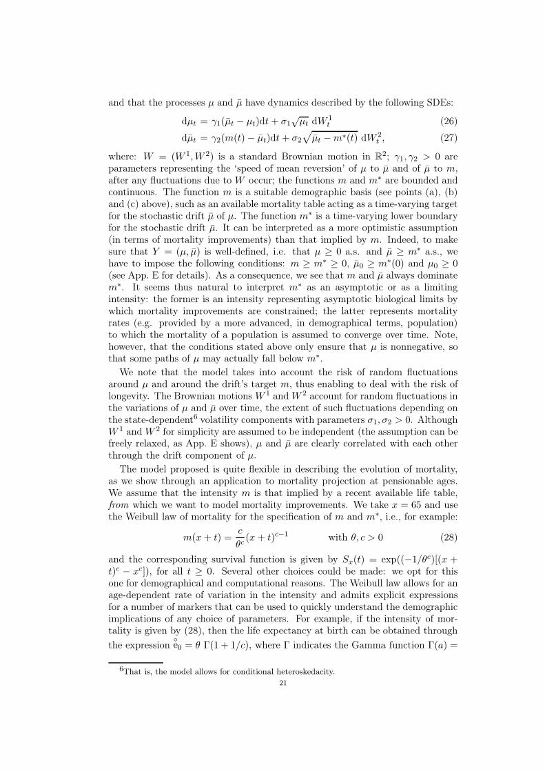
where: W = (W 1,W 2) is a standard Brownian motion in R2; γ1, γ2 > 0 areparameters representing the ‘speed of mean reversion’ of µ to µ and of µ to m,after any fluctuations due to W occur; the functions m and m∗ are bounded andcontinuous. The function m is a suitable demographic basis (see points (a), (b)and (c) above), such as an available mortality table acting as a time-varying targetfor the stochastic drift µ of µ. The function m∗ is a time-varying lower boundaryfor the stochastic drift µ. It can be interpreted as a more optimistic assumption(in terms of mortality improvements) than that implied by m. Indeed, to makesure that Y = (µ, µ) is well-defined, i.e. that µ ≥ 0 a.s. and µ ≥ m∗ a.s., wehave to impose the following conditions: m ≥ m∗ ≥ 0, µ0 ≥ m∗(0) and µ0 ≥ 0(see App. E for details). As a consequence, we see that m and µ always dominatem∗. It seems thus natural to interpret m∗ as an asymptotic or as a limitingintensity: the former is an intensity representing asymptotic biological limits bywhich mortality improvements are constrained; the latter represents mortalityrates (e.g. provided by a more advanced, in demographical terms, population)to which the mortality of a population is assumed to converge over time. Note,however, that the conditions stated above only ensure that µ is nonnegative, sothat some paths of µ may actually fall below m∗.

We note that the model takes into account the risk of random fluctuationsaround µ and around the drift’s target m, thus enabling to deal with the risk oflongevity. The Brownian motions W 1 and W 2 account for random fluctuations inthe variations of µ and µ over time, the extent of such fluctuations depending onthe state-dependent6 volatility components with parameters σ1, σ2 > 0. AlthoughW 1 and W 2 for simplicity are assumed to be independent (the assumption can befreely relaxed, as App. E shows), µ and µ are clearly correlated with each otherthrough the drift component of µ.

The model proposed is quite flexible in describing the evolution of mortality,as we show through an application to mortality projection at pensionable ages.We assume that the intensity m is that implied by a recent available life table,from which we want to model mortality improvements. We take x = 65 and usethe Weibull law of mortality for the specification of m and m∗, i.e., for example:

m(x + t) =c

θc(x + t)c−1 with θ, c > 0 (28)

and the corresponding survival function is given by Sx(t) = exp((−1/θc)[(x +t)c − xc]), for all t ≥ 0. Several other choices could be made: we opt for thisone for demographical and computational reasons. The Weibull law allows for anage-dependent rate of variation in the intensity and admits explicit expressionsfor a number of markers that can be used to quickly understand the demographicimplications of any choice of parameters. For example, if the intensity of mor-tality is given by (28), then the life expectancy at birth can be obtained through

the expressione0 = θ Γ(1 + 1/c), where Γ indicates the Gamma function Γ(a) =

6That is, the model allows for conditional heteroskedacity.

21

∫∞0 e−tta−1dt (with a > 0). Moreover, simple calculus yields that the life ex-

pectancy at age x can be expressed asex = θ[Γ(1+1/c)−γ(1+1/c, (x/θ)c)], where

γ(a, y) =∫ y

0 e−tta−1dt is the Incomplete-Gamma function (e.g. Abramowitz andStegun, 1974, Sec. 6).

We assume that x∗ = 114 is the age at which no one survives, consistentlywith the annuitants life table RG48. We then fit a Weibull survival functionto the projected table COH48 and use the corresponding Weibull intensity asour assumption m. We set an asymptotic Weibull intensity m∗ which is lowenough to allow fluctuations of µ below m, yet large enough to prevent mortalityimprovements from being unreasonable. Tab. 3 reports the Weibull parameters(c, θ), relative to the demographic basis m, the parameter values (c∗, θ∗), relativeto m∗, and the parameters (c0, θ0) relative to the ‘initial’ mortality level µ0, i.e.that of a generation successive to the 1948 one. The demographic meaning of theparameters is synthesized by the life expectancy at age 65. One should think of mas representing a recent (latest) available life table, and regard µ0 as representingan estimate of the intensity of mortality of an individual aged 65 belonging tothe cohort object of projection.

The values of the drift and volatility parameters are all quoted in Tab. 3 exceptγ2, which has been allowed to vary for sensitivity analysis purposes. Fig. 4 depictsseveral survival functions obtained with γ2 ranging from 0.50 (lowest rectangular-ization effect) to 0.05 (greatest rectangularization effect). The survival functionsrelative to m and to the projected table RG48 (to be used as a benchmark) arealso depicted. The effect of the parameter choices on death curves is shown inFig. 5, where one can appreciate the joint rectangularization and expansion effecton the projected density surface.

< table 3 about here >

< figure 4 about here >

< figure 5 about here >

7. Conclusion

In this work we have shown how mortality can be modeled stochastically in orderto provide a rich and flexible framework for actuarial valuations. We have ex-ploited the parallel between life insurance business and credit-sensitive securities,first pointed out in Artzner and Delbaen (1995). By using affine jump-diffusionsas driving processes for the evolution of demographic and financial risk factors,we have demonstrated how actuarial valuations can deal simultaneously with dif-ferent sources of risks. In particular, we have provided closed-form (up to ODEssolution) expressions for the (fair) value of a number of life insurance contracts,either traditional, indexed and unit-linked. The Embedded Value Method, apopular actuarial valuation technique, has been looked at in the context of fairvalue accounting, in order to understand how risk-adjusted discount rates trans-late into adjustments to best-estimate assumptions and vice-versa. Finally, twoaffine models for the intensity of mortality have been proposed, paying particular

22

attention to the demographic meaning of their parameters and to their abilityin capturing the dynamics of mortality evolution. Examples of mortality pro-jections at old ages have been provided, showing how the models proposed canhandle effectively the risk of longevity.

23

References

Abbink, M. and M. Saker (2002). Getting to grips with fair value. Staple InnActuarial Society, London.

Abramowitz, M. and I. Stegun (1974). Handbook of Mathematical Functions.Dover Publications, New York.

Artzner, P. and F. Delbaen (1995). Default risk insurance and incomplete mar-kets. Mathematical Finance, vol. 5(3):187–195.

Bacinello, A. and S. Persson (2002). Design and pricing of equity-linked life insur-ance under stochastic interest rates. The Journal of Risk & Insurance, vol. 3(2):6–21.

Bakshi, G. and D. Madan (2000). Spanning and derivative security valuation.Journal of Financial Economics, vol. 55(2):205–238.

Bakshi, G., C. Cao and Z. Chen (1997). Empirical performance of alternativeoption pricing models. Journal of Finance, vol. 52(5):2003–2049.

Bates, D. (2000). Post-87’ crash fears in S&P500 futures options. Journal of

Econometrics, vol. 94(1-2):181–283.

Biffis, E. (2003). Affine processes in mortality modelling: an actuarial application.Quaderno n. 156, Department of Applied Mathematics, University of Trieste.

Biffis, E. and P. Millossovich (2004). The fair value of guaranteed annuity options.Quaderno n. 162, Department of Applied Mathematics, University of Trieste.

Billingsley, P. (1995). Probability and Measure. Wiley, New York, third edn.

Bowers, N., H. Gerber, J. Hickman, D. Jones and C. Nesbitt (1997). Actuarial

Mathematics. The Society of Actuaries, Schaumburg, Illinois, second edn.

Brémaud, P. (1981). Point Processes and Queues - Martingale Dynamics.Springer-Verlag, New York.

Collins, S. and D. Keeler (1993). Analysis of life company financial performance.Staple Inn Actuarial Society, London.

Cox, J., J. Ingersoll and S. Ross (1985). A theory of the term structure of interestrates. Econometrica, vol. 53(2):385–408.

Dahl, M. (2004). Stochastic mortality in life insurance: Market reserves andmortality-linked insurance contracts. Insurance: Mathematics & Economics,vol. 35(1):113–136.

Dai, Q. and K. Singleton (2000). Specification analysis of affine term structuremodels. Journal of Finance, vol. 55(5):1943–1978.

Deelstra, G. and F. Delbaen (1998). Convergence of discretized stochastic (in-terest rate) processes with stochastic drift term. Applied Stochastic Models and

Data Analysis, vol. 14(1):77–84.

Duffie, D. (2001). Dynamic Asset Pricing Theory . Princeton University Press,Princeton, third edn.

Duffie, D. and R. Kan (1996). A yield-factor model of interest rates. Mathematical

Finance, vol. 6(4):379–406.

Duffie, D., J. Pan and K. Singleton (2000). Transform analysis and asset pricingfor affine jump-diffusions. Econometrica, vol. 68(6):1343–1376.

24

Duffie, D., D. Filipovič and W. Schachermayer (2003). Affine processes andapplications in finance. Annals of Applied Probability , vol. 13(3):984–1053.

Eraker, B., M. Johannes and N. Pohlson (2003). The impact of jumps in volatilityand returns. Journal of Finance, vol. 58(3):1269–1300.

Filipovič, D. (2001). Time-inhomogeneous affine processes. Forthcoming in Sto-

chastic Processes and Their Applications.

Grandell, J. (1976). Doubly Stochastic Poisson Processes. Springer-Verlag, NewYork.

Heston, S. (1993). A closed-form solution for options with stochastic volatilitywith applications to bond and currency options. Review of Financial Studies,vol. 6(2):327–343.

IASB (2001). Draft Statement of Principles. International Accounting StandardsBoard. Available at: www.iasb.org.uk.

IASB (2004). International Financial Reporting Standard n. 4 . InternationalAccounting Standards Board.

Jeanblanc, M. and M. Rutkowski (2000). Modeling of default risk: an overview.In J. Yong and R. Cont (eds.), Mathematical Finance: Theory and Practice, pp.171–269. Higher Education Press, Beijin.

Kallenberg, O. (2002). Foundations of Modern Probability . Springer-Verlag, NewYork, second edn.

Karatzas, I. and S. E. Shreve (1991). Brownian Motion and Stochastic Calculus.Springer-Verlag, New York, second edn.

Keyfitz, N. (1985). Applied Mathematical Demography . Springer-Verlag, NewYork, second edn.

Lando, D. (1998). On Cox processes and credit risky securities. Review of Deriva-

tives Research, vol. 2(2-3):99–120.

MacDonald, A., A. Cairns, P. Gwilt and K. Miller (1998). An internationalcomparison of recent trends in population mortality. British Actuarial Journal ,vol. 4(1):3–141.

Milevsky, M. and S. Promislow (2001). Mortality derivatives and the option toannuitise. Insurance: Mathematics & Economics, vol. 29(3):299–318.

Olivieri, A. (2001). Uncertainty in mortality projections: an actuarial perspective.Insurance: Mathematics & Economics, vol. 29(2):231–245.

Pitacco, E. (2003a). Longevity risk in living benefits. In E. Fornero and E. Luciano(eds.), Developing an Annuity Market in Europe. Edward Elgar Publishing Ltd.

Pitacco, E. (2003b). Survival models in actuarial mathematics: from Halley tolongevity risk. Quaderno n. 2, Department of Applied Mathematics, Universityof Trieste. Forthcoming in Insurance: Mathematics & Economics.

Protter, P. (2004). Stochastic Integration and Differential Equations. Springer-Verlag, Heidelberg, second edn.

Schönbucher, P. (2003). Credit Derivatives Pricing Models. Wiley Finance.

Scott, L. (1997). Pricing stock options in a jump-diffusion model with stochasticvolatility and interest rates: Application of Fourier inversion methods. Mathe-

matical Finance, vol. 7(4):413–426.

25

Sheard, M. (2000). Summary and comparison of approaches used to measure lifeoffice values. Staple Inn Actuarial Society, London.

Vasicek, O. (1977). An equilibrium characterization of the term structure. Journal

of Financial Economics, vol. 5(2):177–188.

Wilmoth, J. and S. Horiuchi (1999). Rectangularization revisited: Variability ofage at death within human populations. Demography , vol. 36(4):475–495.

Appendix A. Affine Processes

We now specify explicitly the affine dependence on X ∈ Rn of the coefficients appearingin the SDE (2) of Sec. 3. In particular, we have:

δ(t, x) = d0(t) + d1(t)x(σ(t, x)σ(t, x)T

)i,j

= (V0(t))i,j + (V1(t))i,j · x i, j = 1, . . . , n

κ(t, x) = k0(t) + k1(t) · x

where c·d =∑n

j=1 cjdj for all c, d ∈ Cn. The functions d.= (d0, d1), V

.= (V0, V1) and k

.=

(k0, k1) are defined on [0,∞), take values respectively in Rn×Rn×n, Rn×n×Rn×n×n andR×Rn, and are assumed to be bounded and continuous. Moreover, the time-dependentjump-size distribution νt is determined by its Laplace transform: θ(t, c) =

∫Rn ec·zdνt(z),

defined for t ∈ [0,∞), c ∈ Cn and such that the integral is finite. The transform θ andthe functions d, V and k completely determine the distribution of X , once an initialcondition X0 is given.

Focusing now on the transform (3), when (d,V ,k,θ) and the affine function Λ are‘extended well-behaved’ in the sense defined by Duffie, Pan and Singleton (2000, App. A),the functions α(·) .

= α(·; a, T ) and β(·) .= β(·; a, T ) satisfy the following ODEs:

β(t) = λ1(t) − d1(t)Tβ(t) − 1

2β(t)TV1(t)β(t) − k1(t) [θ(t, β(t)) − 1] (A.1)

α(t) = λ0(t) − d0(t) · β(t) − 1

2β(t)TV0(t)β(t) − k0(t) [θ(t, β(t)) − 1] (A.2)

with boundary conditions α(T ) = 0 and β(T ) = a, while the functions α(·) .= α(·; a, b, c, T )

and β(·) .= β(·; a, b, T ) solve the ODEs:

˙β(t) = −d1(t)

Tβ(t) − β(t)TV1(t)β(t) − k1(t)[Θ(t, β(t)) · β(t)

](A.3)

˙α(t) = −d0(t) · β(t) − β(t)TV0(t)β(t) − k0(t)[Θ(t, β(t)) · β(t)

](A.4)

with boundary conditions α(T ) = c and β(T ) = b, where Θ(t, c) denotes the gradient ofθ(t, c) with respect to c ∈ Cn, i.e. Θ(t, c) =

∫Rn c exp(c · z)νt(dz). We remind that for all

c, d ∈ Cn the vector in Cn with k-th element∑

i,j ci(V1(t))ijkdj is denoted by cTV1(t)d.

Solutions to the ODEs above can be found explicitly in some cases, through the use ofnumerical methods in other cases. The choice of a jump distribution with an explicitlyknown or easily computed transform θ is clearly important for computational tractability.

Appendix B. No-arbitrage restrictions

We provide here the no arbitrage constraints for any risky security of the form S =exp(Xi) with affine dividend yield ζ(t, Xt) = q0(t) + q1(t) ·Xt, as considered in Sec. 4.1.By applying Itô’s formula to S (e.g. Protter, 2004, pp. 78-79) and forcing the drift to be

26

equal to r − ζ under Q, we get the following conditions, on the lines of Duffie, Pan andSingleton (2000, Sec. 3.1):

(d1(t))i = ρ1(t) − q1(t) −1

2(V1(t))i,i − k1(t) [θ(t, ε(i)) − 1]

(d0(t))i = ρ0(t) − q0(t) −1

2(V0(t))i,i − k0(t) [θ(t, ε(i)) − 1]

where ε(i) indicates the vector in Rk with all null components but the i-th, which isequal to 1.

Appendix C. Construction of the random time of death

We take as given a probability space (Ω,F , P) and consider a filtration G satisfying theusual conditions and such that G∞ ⊂ F . We assume that a nonnegative G-predictable

process µ is given satisfying∫ t

0 µsds < ∞ a.s. for all t > 0. We then fix an exponentialrandom variable Φ with parameter 1, independent of G∞, and define the random timeof death τ as the first time when the process

∫ ·

0µsds is above the random level Φ, i.e.we

set:

τ.= inf

t ∈ R+ :

∫ t

0

µsds ≥ Φ

.

We note that τ > T = ∫ T

0 µsds < Φ, for T ≥ 0. Thus, for T ≥ t ≥ 0, by usingthe law of iterated expectations and by exploiting the independence of Φ and GT , oneobtains that:

P (τ > T |Gt) = E

[P

(Φ >

∫ T

0

µsds∣∣∣GT

) ∣∣∣Gt

]= E

[e−

∫T

0µsds

∣∣∣Gt

]. (C.1)

Note that the same result holds for 0 ≤ T < t. The filtration F = (F)t≥0 of Sec. 4.3 isfinally obtained by defining Ft

.= Gt ∨ Ht, where Ht = σ(Iτ≤s; 0 ≤ s ≤ t). We now

observe that τ > t is an atom of Ht. We can thus verify (using a slight extensionof Billingsley, 1995, ex. 34.4, p. 455) that we have constructed a doubly stochastic F-stopping time driven by G ⊂ F in the following way:

P (τ > T |GT ∨ Ft) = Iτ>tE[Iτ>T|GT ∨Ht

]= Iτ>t

P (τ > T ∩ τ > t|GT )

P (τ > t|GT )=

= Iτ>tP (τ > T |GT )

P (τ > t|GT )= Iτ>te

−∫

T

tµsds,

Finally, we observe that the independence of Φ and GT , and in particular of Φ and

Gt ∨ σ(exp(−∫ T

0 µsds)), enables to write from (C.1):

E[e−

∫T

0µsds

∣∣∣Gt ∨ σ(Φ)]

= E[e−

∫T

0µsds

∣∣∣Gt

],

for all T ≥ t ≥ 0. But Gt ⊂ Ft ⊂ Gt ∨ σ(Φ) and therefore also the following holds:

E[e−

∫T

0µsds

∣∣∣Ft

]= E

[e−

∫T

0µsds

∣∣∣Gt

].

Similar reasoning yields that we can replace the conditioning on Ft with that on Gt inProp. 5.1 and 5.2.

We do not take G ∨ σ(Φ) as our reference filtration F because, if that were the case,the stopping time τ would be predictable and would not admit an intensity. The con-struction outlined ensures instead that τ is a totally inaccessible stopping time, a conceptintuitively meaning that the insured’s death arrives as a total surprise to the insurer (seeProtter, 2004, Ch. III.2, for details).

27

Appendix D. Poisson-Gaussian process: explicit solutions

Since for model (24) the factorization exploited in (19) holds, we can focus on the randomcomponent η

1Y , where Y has dynamics described through the SDE (25). The parameters

of App. A have the following specification in this particular case:

d0(t) = γy(t) d1 = −γ V0 = σ2 V1 = 0

k0 = k k1 = 0 λ = (0, η1)

Moreover, the jump transform θ is given by:

θ(c) =

∫ ∞

0

1

je−(c+ 1

j )zdz =1

1 + jcfor <(c) > −1

j,

where <(c) denotes the real part of c ∈ C. We can solve (A.1) with boundary conditionβ(T ) = 0, thus getting:

β(t) = η1

e−γ(T−t) − 1

γ,

which can be plugged into (A.2) to obtain (using the condition α(T ) = 0 and integrating):

α(t) =σ2

2γ2

[η2

1(T − t) + η

1β(t) − γ

2β2(t)

]− kjη

1

jη1− γ

(T − t)+

− k

jη1− γ

log |1 + jβ(t)| + γ

∫ T

t

y(u)β(u)du.

Appendix E. Bidimensional square-root diffusion: technical

conditions

We write explicitly the parameters of App. A relative to the dynamics of the processY = (µ, µ)T described by the SDEs (26)-(27). Specifically, we have:

d0(t) =

[0

γ2m(t)

]d1 =

[−γ1 γ1

0 −γ2

]

V0(t) =

[0 00 −σ2

2m∗(t)

]V1 =

σ21 00 00 00 σ2

2

κ = (0, (0, 0)T) λ = (0, (1, 0)T)

These can be used to solve the ODEs (A.1) to (A.4) when implementing the model.

We now move on to the technical conditions ensuring that the process Y = (µ, µ)T

is well-defined. Let us first focus on the square-root process µ. Since the functionf(t, x) = σ2

√|x − m∗(t)| (with (t, x) ∈ R+ × R) satisfies the Hölder condition:

|f(t, x) − f(t, y)| ≤ K√|x − y|,

with K a positive constant, then strong uniqueness holds for all the SDEs of the type(see Karatzas and Shreve, 1991, pp. 291,310):

dµt = k2(m(t) − µt)dt + σ2

√|µt − m∗(t)|dW

(2)t , (E.1)

We can therefore use a comparison theorem argument to compare any solution to (E.1)with the trivial solution µ = m∗ to the following SDE:

dµt = k2(m∗(t) − µt)dt + σ2

√|µt − m∗(t)|dW

(2)t

Specifically, we have that imposing m ≥ m∗ and µ0 ≥ m∗(0) is sufficient to ensure thatµ ≥ m∗ a.s., thus justifying the SDE (27) (e.g Karatzas and Shreve, 1991, p. 293).

28

We can now focus on the SDE (26) describing the dynamics of µ. Since µ is a

measurable adapted process and∫ t

0µudu < ∞ for all t ∈ R+, we have that, if µ ≥ 0 and

µ0 ≥ 0, then µ is well-defined and µ ≥ 0 (see Deelstra and Delbaen, 1998). We can thentake m ≥ m∗ ≥ 0, µ0 ≥ m∗(0) and µ0 ≥ 0, thus ensuring that Y is well-defined andthat the intensity of mortality µ never becomes negative almost surely. We note that norequirement need to be made on the correlation between µ and µ.

29

0 20 40 60 80 100 1200

0.1

0.2

0.3

0.4

0.5

0.6

0.7

0.8

0.9

1SIM31SIM51SIM61SIM71SIM81SIM92

Figure 1: Joint effect of rectangularization and expansion on the survival function.

30

20 30 40 50 60 70 80 90 100 110 1200

0.005

0.01

0.015

0.02

0.025

0.03

0.035

0.04SIM31SIM51SIM61SIM71SIM81SIM92

Figure 2: Joint effect of rectangularization and expansion on the curve of deaths.

31

Projection m(t) η1 γ y(t) y(x∗ − x) σ j k Y0

A SIM92 0.5 0.6 -0.005000 -0.0050 0.100 0.100 0.100 -0.016

B SIM92 0.6 0.6 -0.000900 -0.0009 0.050 0.050 0.400 -0.016

C Coh48 0.6 0.8 -0.001400 t -0.0700 0.050 0.005 0.100 -0.009

D Coh48 0.6 0.6 -0.001800 t -0.0900 0.075 0.020 0.200 -0.009

E Coh48 0.7 0.6 -0.000521 t2 -1.2500 0.070 0.020 0.250 -0.009

Table 1: Parameter values for the Poisson-Gaussian model.

32

Life Tablee65 H65 ∆ δ Y∞

SIM92 14.639 0.462 - - -

Coh48 17.799 0.365 - - -

RG48 19.128 0.333 - - -

A 16.871 0.406 -0.001400 -33.00% -0.0108

B 18.215 0.356 -0.002200 -52.87% -0.0205

C 19.020 0.354 -0.000346 -18.81% -0.0567

D 20.955 0.298 -0.000895 -48.61% -0.0565

E 20.221 0.306 -0.000687 -37.32% -0.7075

Table 2: Demographic measures for life tables and and parameter choices of Tab. 1.

33

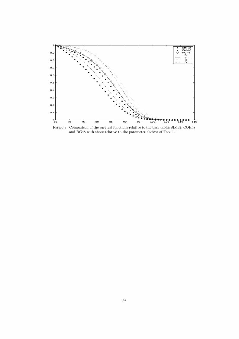
65 70 75 80 85 90 95 100 105 110 1150

0.1

0.2

0.3

0.4

0.5

0.6

0.7

0.8

0.9

1SIM92Coh48RG48 A B C D

Figure 3: Comparison of the survival functions relative to the base tables SIM92, COH48and RG48 with those relative to the parameter choices of Tab. 1.

34

m m(0) m∗

c 10.841 c0 11 c∗ 13

θ 86.165 θ0 90 θ∗ 100e65 18.345

e65 21.704

e65 31.130

k1 0.6 σ1 0.15 σ2 0.35

Table 3: Parameter values for the bidimensional square-root diffusion intensity model.

35

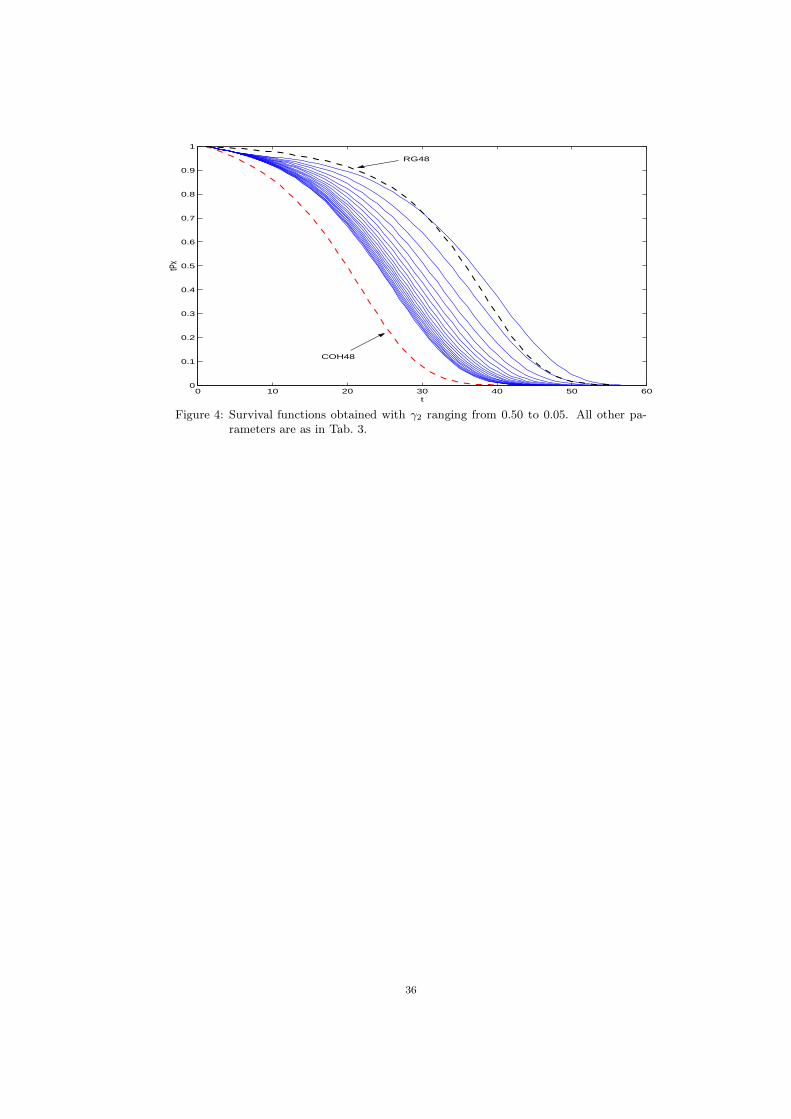
0 10 20 30 40 50 600

0.1

0.2

0.3

0.4

0.5

0.6

0.7

0.8

0.9

1

t

tPx

COH48

RG48

Figure 4: Survival functions obtained with γ2 ranging from 0.50 to 0.05. All other pa-rameters are as in Tab. 3.

36

0.05

0.1

0.15

0.2

0.25

0.3

0.35

0.4

0.45

0.5 010

2030

4050

60

0

0.01

0.02

0.03

0.04

0.05

tγ2

f 65(t

)

Figure 5: Density surface obtained with γ2 ranging from 0.50 to 0.05. All other param-eters are as in Tab. 3.

37