ae2610 aerodynamic forces in subsonic wind...

Copyright 1999-2000, 2002, 2009, 2015, 2018, 1

by H. McMahon, J. Jagoda, N. Komerath, and J. Seitzman. All rights reserved.

AE2610 Introduction to Experimental Methods in Aerospace

AERODYNAMIC FORCES ON A WING IN A SUBSONIC WIND TUNNEL

Objectives

The primary objective of this experiment is to familiarize the student with measurement of

aerodynamic forces in a wind tunnel. A six-component sting balance will be used to measure

forces and moments on a rectangular (two-dimensional) wing with an adjustable plain flap. In

addition, the student will become acquainted with the operation of a subsonic wind tunnel,

including use of a Pitot-static probe and pressure transducer to measure wind speed.

Background

a) Aerodynamics of a Wing

i) Forces and Moments − In general, a body moving through a fluid is subject to three force

and three moment components. The primary force components on an aerodynamic body, and

in particular a wing, are lift and drag. Lift is the force component that is perpendicular to the

oncoming flow direction, and drag is the component parallel to the flow (see Figure 1). Lift is

generally considered positive when in a direction “upward” (opposing gravity), while drag is

normally positive in the flow direction (i.e., tending to slow down the body). The third

component is the called the side force. For objects symmetric about the side force axis and

moving straight into the flow, there should be no side force. Side forces on a wing usually

come about when an aircraft is turning or not flying into the wind.

The three moments are: the pitching, roll, and yaw moments (see Figure 1). The pitching

moment is around an axis parallel to the direction of the side force, and would act to change

the pitch or angle of attack () of the lift body. The roll moment is around an axis in the drag

direction, while the yaw moment acts around the lift axis. For most wings flying into the wind,

the pitching moment is the dominant component. It is customary to define the pitching

moment about the aerodynamic center; the point at which the pitching moment does not vary

with lift coefficient, i.e., angle of attack.

The magnitudes of the aerodynamic forces and moments depend primarily on the shape of

the body, the speed and orientation of the body with respect to the fluid, and certain properties

of the fluid. For a rectangular wing, lift primarily depends on the curvature (camber1) of its

1 The camber line of a wing’s cross-section connects the midway points between the upper and lower surfaces.

AE 2610 Aerodynamic Forces in Subsonic Wind Tunnel

2

cross-section, the angle of attack, the flow speed, and the density of air. The shape of the

wing’s cross-section is known as an airfoil.

The thin airfoil inviscid flow model2 (also called “thin airfoil theory”) predicts that lift

increases with increasing positive (concave downward) camber or with rearward movement of

the location of the maximum camber. In a “real” viscous airflow, this is also true at moderate

angles of attack. Thus, the maximum value of the lift coefficient attainable with any airfoil

increases with increasing camber. This is of great benefit, since the higher the maximum lift

coefficient the lower the stalling speed. Also, the effective camber of an airfoil can be varied

by deflecting a segment of the airfoil such as a flap or aileron. It may be shown that, for a

given amount of deflection, the change in lift coefficient is larger if the deflection occurs at the

trailing edge rather than at the leading edge. Hence, flaps and ailerons are fitted at the trailing

edge of an airfoil or wing. Additionally, thin airfoil theory predicts that the aerodynamic center

of an airfoil is located one-quarter of a chord length behind its leading edge.

The rectangular wing used in this experiment (see Table 1 for dimensions) is fitted with a

plain trailing edge flap. Aerodynamics forces on the airfoil will be measured as a function of

wing angle of attack and flap deflection angle. The lift results will show if increased flap

deflection has the expected effect, while the drag results will show whether an increase in lift

at a fixed angle of attack by means of a flap deflection is accompanied by any corresponding

drag change. If there is a drag increase this is not necessarily a disadvantage. For example,

during landing the higher engine power required to compensate for the drag increase will

minimize engine acceleration time in the event of a missed approach.

ii) Aerodynamics Coefficients − Aerodynamics forces on a wing are typically normalized and

expressed as aerodynamic force coefficients. For example, the lift coefficient (CL), drag

coefficient (CD) and pitching moment coefficient (CM) are defined as

Sq

LCL

(1)

Sq

DCD

(2)

Scq

MCM

(3)

2 See for example, Anderson's Fundamentals of Aerodynamics.


3

where L is the lift force, D is the drag force, M is the pitching moment, S is the plan form area

of the wing, c is the chord length (see Figure 1), and q is the dynamic pressure. For our

rectangular wing, S = c b, where b is the span (tip-to-tip length) of the wing.

Thin airfoil theory predicts that CL for a symmetric airfoil, i.e., where the chord and

camber lines are the same (also known as a zero camber airfoil) that also has infinite span is

given by

2LC (4)

This expression is valid only for small and moderate angles of attack. At sufficiently large

angles of attack, the flow over the wing no longer follows the surface, and the wing’s lift

coefficient begins to drop, i.e., the wing stalls.

The dynamic pressure q is given by

2

21 v q (5)

where is the density of the approaching flow and v is its speed (relative to the body/wing).

This is called the dynamic pressure because according to Bernoulli's equation (which is valid

for a low speed, constant density flow) it represents the difference between the stagnation (or

total) pressure and static pressure of a flow, i.e.,

2

21 v ppo (6)

The static pressure is the pressure one would measure if moving with the flow (or without

requiring a change in the flow velocity), while stagnation pressure is the static pressure that the

flow would achieve if it was slowed (in an ideal manner) to zero velocity.

For an ideal gas, the density is given by

RT

p (7)

Here p is the (absolute) pressure, T is the (absolute) temperature, and R is the gas constant for

the specific gas.

b) Sensors and Transducers

i) Sting Balance − The force-measuring device to be used in these experiments is a sting

balance mounted on a model positioning system (MPS) that controls both pitch and yaw

angles. Wind tunnel force balances can be categorized into two basic types: external and

internal. The force transducers for external balances are located outside the wind tunnel test


4

section, and the aerodynamic forces must be mechanically transmitted from the test body in

the wind tunnel to the balance outside. Internal balances have their force measuring unit within

the wind tunnel, and thus provide a more direct measurement of the aerodynamic forces. The

AerolabsTM internal balance (Figure 2) employed in our wind tunnel uses strain gauges

mounted within a rod cut from a single piece of precipitation-hardened stainless steel with a

protective sheath to protect the fragile foil strain gauges. The strain gauges are connected to

electronics (including wheatstone bridges), which are in turn connected to a computer data

acquisition system located in the wind tunnel control room. The Aerolab system will acquire

5000 samples every 100 ms and report the average. By setting the dwell time of the MPS, you

can set the number of measurements that will be recorded at each angle of attack (e.g., a dwell

time of 1 second would result in 10 measurements).

Two procedures are required to convert the voltage outputs from the strain gauge system

into accurate measurements of the aerodynamics forces (and moments). First, the strain gauges

must be calibrated. This is accomplished using an attachment of known mass that can be

connected to the balance. Second, any forces transmitted to the balance that are not

produced by the wing must be removed. In this experiment, there is a support structure that

connects the balance to the wing (see Figure 3). This support structure can produce its own

aerodynamics forces. In addition, even with the wind tunnel off, the weight of the structure and

wing will load the balance. Removing these wind-off (or tare) loads is known as taring the

system.

If the data are to be meaningful, each test run must be carried out at a (nearly) constant

value of wind tunnel dynamic pressure. Ideally, the magnitude of the aerodynamics force

coefficients would be independent of the magnitude of the dynamic pressure. In reality, this

assumption might not be completely accurate, so the dynamic pressure should be held constant

during a particular data-taking run so that the coefficients will not be influenced by changes in

freestream conditions. The speed of the fan that drives the wind tunnel is nominally held

constant by the fan’s motor control system. This should produce a nearly constant wind tunnel

dynamic pressure. (If necessary, the dynamic pressure can be manually adjusted with the

tunnel speed control.)

ii) Pitot-Static Probe - In addition, a second data acquisition system will simultaneously

acquire and store the dynamic pressure during the experiment. The dynamic pressure is

measured directly by means of a Pitot-static probe mounted in the freestream. The probe has

one hole facing directly into the wind tunnel flow and another located so the air flows along

the surface of the hole (see Figure 4). The pressure in the first hole is the stagnation pressure

(po) and the second experiences the static pressure (p). The two holes are connected via long


5

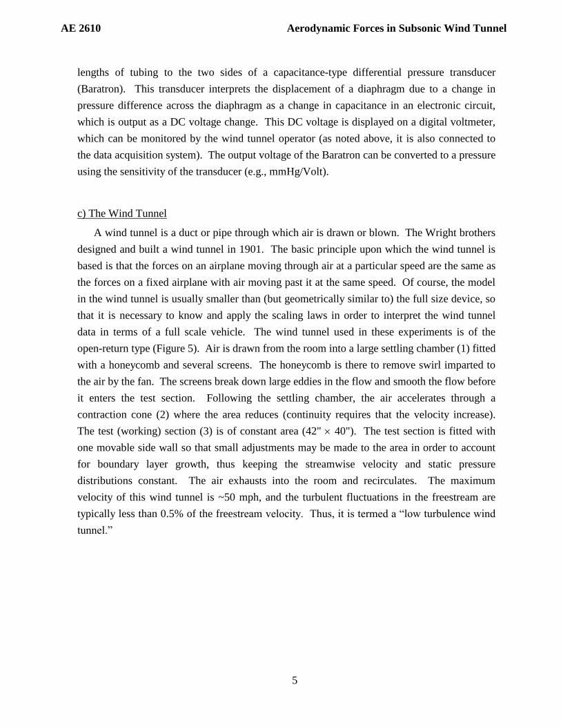
lengths of tubing to the two sides of a capacitance-type differential pressure transducer

(Baratron). This transducer interprets the displacement of a diaphragm due to a change in

pressure difference across the diaphragm as a change in capacitance in an electronic circuit,

which is output as a DC voltage change. This DC voltage is displayed on a digital voltmeter,

which can be monitored by the wind tunnel operator (as noted above, it is also connected to

the data acquisition system). The output voltage of the Baratron can be converted to a pressure

using the sensitivity of the transducer (e.g., mmHg/Volt).

c) The Wind Tunnel

A wind tunnel is a duct or pipe through which air is drawn or blown. The Wright brothers

designed and built a wind tunnel in 1901. The basic principle upon which the wind tunnel is

based is that the forces on an airplane moving through air at a particular speed are the same as

the forces on a fixed airplane with air moving past it at the same speed. Of course, the model

in the wind tunnel is usually smaller than (but geometrically similar to) the full size device, so

that it is necessary to know and apply the scaling laws in order to interpret the wind tunnel

data in terms of a full scale vehicle. The wind tunnel used in these experiments is of the

open-return type (Figure 5). Air is drawn from the room into a large settling chamber (1) fitted

with a honeycomb and several screens. The honeycomb is there to remove swirl imparted to

the air by the fan. The screens break down large eddies in the flow and smooth the flow before

it enters the test section. Following the settling chamber, the air accelerates through a

contraction cone (2) where the area reduces (continuity requires that the velocity increase).

The test (working) section (3) is of constant area (42" 40"). The test section is fitted with

one movable side wall so that small adjustments may be made to the area in order to account

for boundary layer growth, thus keeping the streamwise velocity and static pressure

distributions constant. The air exhausts into the room and recirculates. The maximum

velocity of this wind tunnel is ~50 mph, and the turbulent fluctuations in the freestream are

typically less than 0.5% of the freestream velocity. Thus, it is termed a “low turbulence wind

tunnel.”


6

PRELIMINARY

The following items must be turned in at the start of your lab session.

1. Develop a single equation that gives difference between the stagnation and static pressures

in the wind tunnel flow, i.e., the dynamic pressure q, in units of mm Hg (also called Torr)

as a function of:

u, velocity of the flow (in mph),

Troom, room temperature (in F)

proom, room pressure (in inches of Hg),

and two constants (i.e., numbers like “3.4”).

This means your equation should have only two numbers, and three variables (u, Troom and

proom). You will measure Troom and proom (in the units given) and use this equation to

determine the wind tunnel q (in mm Hg) for a wind speed given in mph. The dynamic

pressure must be expressed in mm Hg since that is the measurement unit of the transducer.

Watch your units, this is part of your grade. Include the development (starting with the

Bernoulli equation) when you turn in the final equation.

2. Turn in a suggested list of 10 angles of attack for making the force and moment

measurements (see item 2 in the Procedure section below). This will save you time in the

lab - and let you leave earlier, if you have thought about what would be good values to test.

In other words, consider at what angles interesting “things” happen to the lift. It may help

to check out (look up) some lift versus angle of attack data for airfoils similar to ours (see

Table 1 for its dimensions). You may want to start out with symmetric airfoils since ours is

symmetric when the flap angle is zero.

PROCEDURE

Please note the sting balance rod can be damaged if large loads are applied –

especially any bending loads – for this reason, great care should be taken when

handling it and your TA should connect the balance to the MPS.

1. Determine the Baratron output voltage (dynamic pressure) required to produce the desired

wind tunnel speed, which is somewhere between 33 and 36 mph, and the angles of attack

your group will use.

2. With the help of the TA, attach the wing support and balance rod to the MPS without the

wing.


7

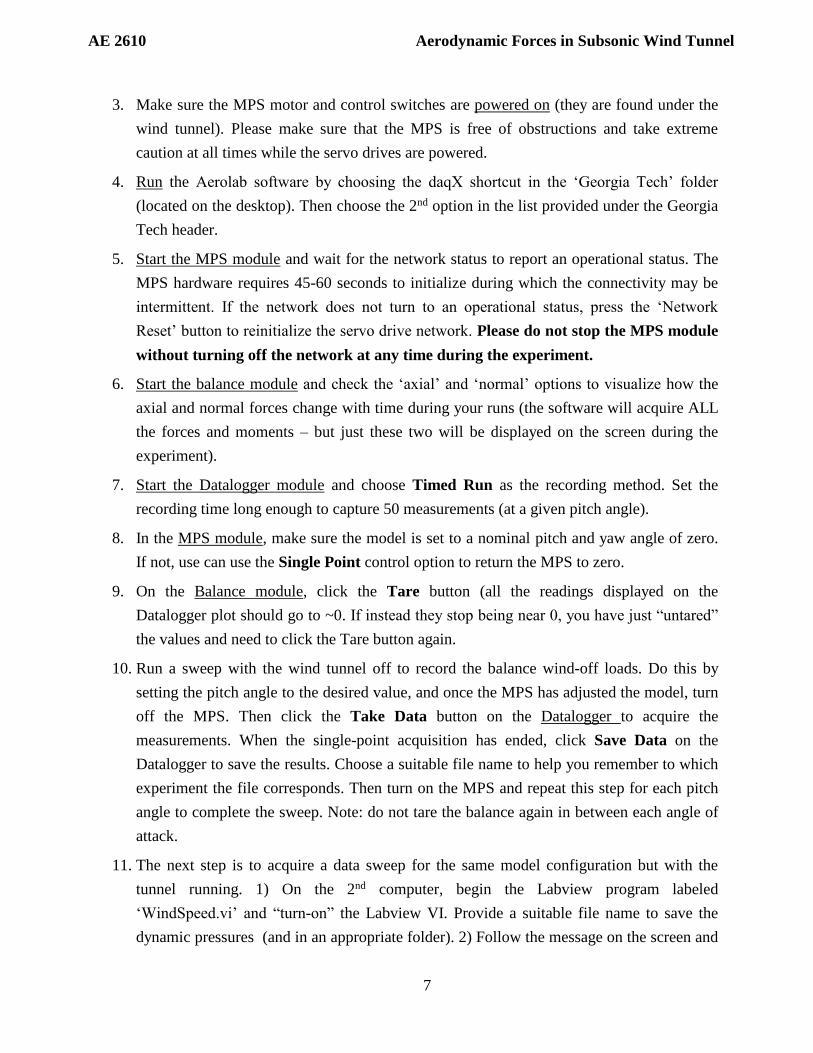
3. Make sure the MPS motor and control switches are powered on (they are found under the

wind tunnel). Please make sure that the MPS is free of obstructions and take extreme

caution at all times while the servo drives are powered.

4. Run the Aerolab software by choosing the daqX shortcut in the ‘Georgia Tech’ folder

(located on the desktop). Then choose the 2nd option in the list provided under the Georgia

Tech header.

5. Start the MPS module and wait for the network status to report an operational status. The

MPS hardware requires 45-60 seconds to initialize during which the connectivity may be

intermittent. If the network does not turn to an operational status, press the ‘Network

Reset’ button to reinitialize the servo drive network. Please do not stop the MPS module

without turning off the network at any time during the experiment.

6. Start the balance module and check the ‘axial’ and ‘normal’ options to visualize how the

axial and normal forces change with time during your runs (the software will acquire ALL

the forces and moments – but just these two will be displayed on the screen during the

experiment).

7. Start the Datalogger module and choose Timed Run as the recording method. Set the

recording time long enough to capture 50 measurements (at a given pitch angle).

8. In the MPS module, make sure the model is set to a nominal pitch and yaw angle of zero.

If not, use can use the Single Point control option to return the MPS to zero.

9. On the Balance module, click the Tare button (all the readings displayed on the

Datalogger plot should go to ~0. If instead they stop being near 0, you have just “untared”

the values and need to click the Tare button again.

10. Run a sweep with the wind tunnel off to record the balance wind-off loads. Do this by

setting the pitch angle to the desired value, and once the MPS has adjusted the model, turn

off the MPS. Then click the Take Data button on the Datalogger to acquire the

measurements. When the single-point acquisition has ended, click Save Data on the

Datalogger to save the results. Choose a suitable file name to help you remember to which

experiment the file corresponds. Then turn on the MPS and repeat this step for each pitch

angle to complete the sweep. Note: do not tare the balance again in between each angle of

attack.

11. The next step is to acquire a data sweep for the same model configuration but with the

tunnel running. 1) On the 2nd computer, begin the Labview program labeled

‘WindSpeed.vi’ and “turn-on” the Labview VI. Provide a suitable file name to save the

dynamic pressures (and in an appropriate folder). 2) Follow the message on the screen and


8

use the wind tunnel controller to set the wind tunnel to the desired speed. DO NOT hit start

on the Labview program yet!

12. Now you will record the aerodynamic forces with the tunnel on by following the same

procedure outlined in step 10 - HOWEVER this time you will need to synchronize the start

and end points of the acquisition on the Aerolab and Labview software by beginning both

at the same time (this will require two people – one working each computer).

13. Have the TA help with removing the test model from the MPS. Then attach the wing after

setting the flap angle to zero. Then, have the TA help reinstall the model to the MPS.

14. Repeat steps 9-12.

15. Have the TA help with removing the test model from the MPS. Then set the flap angle to

your chosen angle. Then have the TA help reinstall the model to the MPS.

16. Make sure the MPS is set to zero pitch (and zero yaw), and make sure the system is

retared.

17. Repeat step 12 (i.e., a sweep for the chosen wind tunnel speed) at your new flap angle.

18. After the tests are concluded, the appropriate data files will be transferred by the TA’s to

the lab website for later data reduction (as noted below).

DATA TO BE TAKEN

1. You must record the room temperature and barometric pressure in order to set the wind

tunnel speed.

2. Tared forces and moments of the wing support structure at 10 angles of attack.

3. Tared forces and moments of wing and support structure at the same 10 angles of attack.

DATA REDUCTION

1. Remove the support structure loads from the loads acquired with the wing + support

structure to find the wing-only normal force, axial force and pitching moment.

2. Convert the measured forces in the balance reference frame to the wind frame (i.e., convert

to lift and drag).

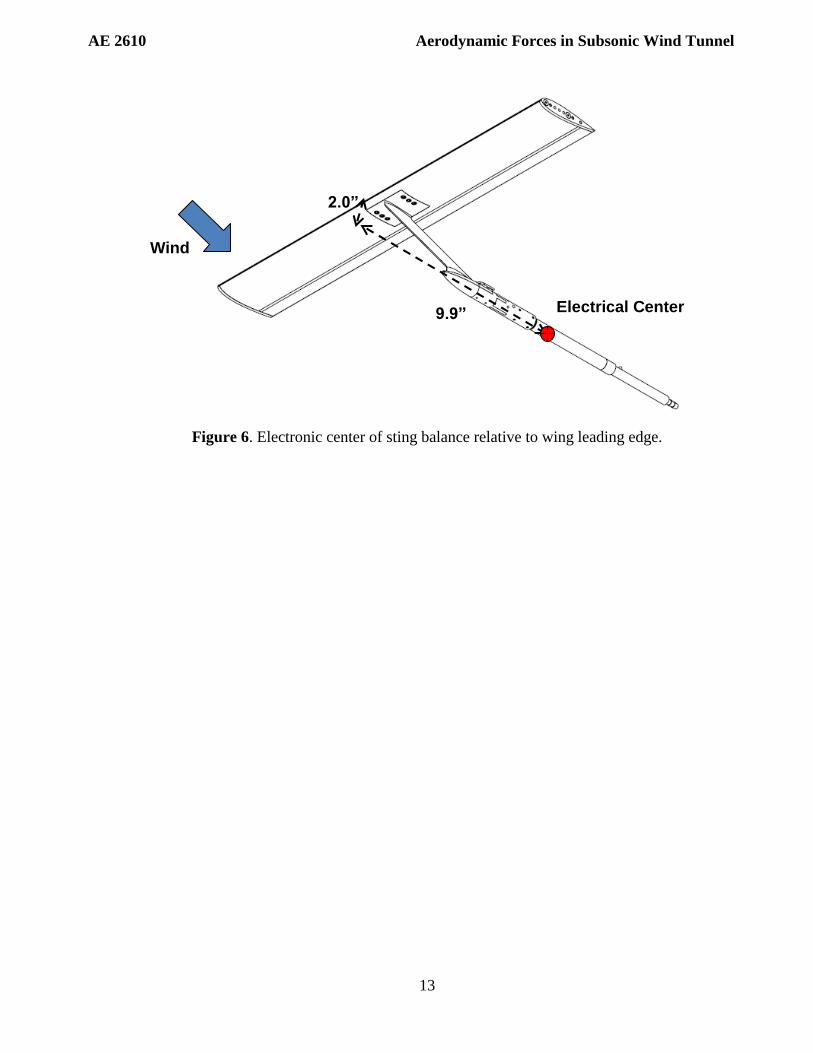
3. Convert the recorded pitch moments about the electrical center of the sting balance to the

(nominal) aerodynamic center of the wing. The electrical center of the sting balance is

located as shown in Figure 6.

4. Express all forces and moments in coefficient form. The chord to be used is the chord of

the wing from the wing leading edge to the flap trailing edge.


9

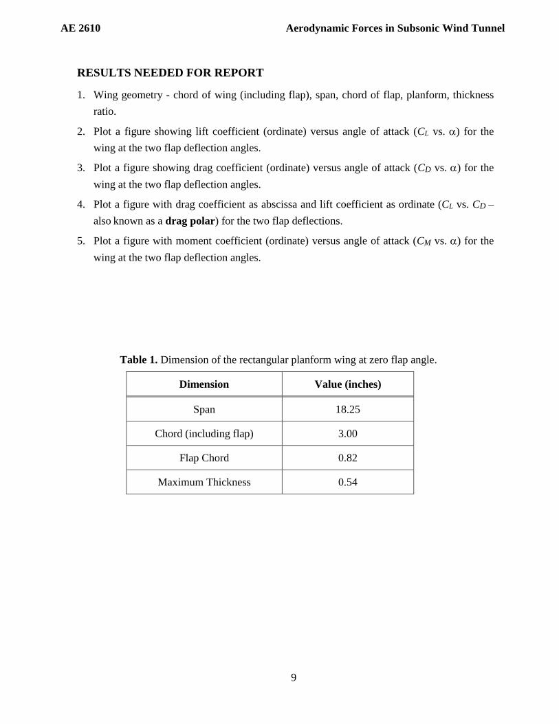
RESULTS NEEDED FOR REPORT

1. Wing geometry - chord of wing (including flap), span, chord of flap, planform, thickness

ratio.

2. Plot a figure showing lift coefficient (ordinate) versus angle of attack (CL vs. ) for the

wing at the two flap deflection angles.

3. Plot a figure showing drag coefficient (ordinate) versus angle of attack (CD vs. ) for the


4. Plot a figure with drag coefficient as abscissa and lift coefficient as ordinate (CL vs. CD –

also known as a drag polar) for the two flap deflections.

5. Plot a figure with moment coefficient (ordinate) versus angle of attack (CM vs. ) for the


Table 1. Dimension of the rectangular planform wing at zero flap angle.

Dimension Value (inches)

Span 18.25

Chord (including flap) 3.00

Flap Chord 0.82

Maximum Thickness 0.54


10

v

Lift

Drag

Chord Line

Pitch

Yaw

Roll

c

Mean Camber

Line

Figure 1. Some of the force and moment components on an airfoil. The angle

of attack () is shown between the chord line and the flow direction.

Figure 2. Schematic of Aerolab internal strain gauge sting balance (shown

without protective sheath) mounted on model positioning system (MPS).


11

Figure 3. Schematic of wing and support structure connected to sting balance

(left – bottom view; right – top view).

v

po

p

Figure 4. Schematic of Pitot-static probe in a wind tunnel.


12

Figure 5. Georgia Tech low turbulence wind tunnel.


13

AF

Wind

Electrical Center 9.9”

2.0”

Figure 6. Electronic center of sting balance relative to wing leading edge.

ae2610 aerodynamic forces in subsonic wind...

Documents