adversarial patrolling with spatially uncertain alarm signals
TRANSCRIPT

Adversarial patrolling with spatially uncertain alarmsignals
Nicola Basilicoa, Giuseppe De Nittisb, Nicola Gattib
aDepartment of Computer Science, University of Milan, Milano, ItalybDipartimento di Elettronica, Informazione e Bioingegneria, Politecnico di Milano, Milano, Italy
Abstract
When securing complex infrastructures or large environments, constant surveil-lance of every area is not affordable. To cope with this issue, a common counter-measure is the usage of cheap but wide–ranged sensors, able to detect suspiciousevents that occur in large areas, supporting patrollers to improve the effectivenessof their strategies. However, such sensors are commonly affected by uncertainty.In the present paper, we focus on spatially uncertain alarm signals. That is, thealarm system is able to detect an attack but it is uncertain on the exact positionwhere the attack is taking place. This is common when the area to be secured iswide such as in border patrolling and fair site surveillance. We propose, to the bestof our knowledge, the first Patrolling Security Game model where a Defender issupported by a spatially uncertain alarm system which non–deterministically gen-erates signals once a target is under attack. We show that finding the optimal strat-egy in arbitrary graphs isAPX–hard even in zero–sum games and we provide two(exponential time) exact algorithms and two (polynomial time) approximation al-gorithms. Furthermore, we analyse what happens in environments with specialtopologies, showing that in linear and cycle graphs the optimal patrolling strategycan be found in polynomial time, de facto allowing our algorithms to be used inreal–life scenarios, while in trees the problem is NP–hard. Finally, we show thatwithout false positives and missed detections, the best patrolling strategy reducesto stay in a place, wait for a signal, and respond to it at best. This strategy is opti-mal even with non–negligible missed detection rates, which, unfortunately, affectevery commercial alarm system. We evaluate our methods in simulation, assessingboth quantitative and qualitative aspects.
Keywords: Security Games, Adversarial Patrolling, Algorithmic Game Theory
Preprint submitted to Artificial Intelligence June 10, 2015
arX
iv:1
506.
0285
0v1
[cs
.AI]
9 J
un 2
015

1. Introduction
Security Games model the task of protecting physical environments as a non–cooperative game between a Defender and an Attacker [1]. These games usuallytake place under a Stackelberg (a.k.a. leader–follower) paradigm [2], where theDefender (leader) commits to a strategy and the Attacker (follower) first observessuch commitment, then best responds to it. As discussed in the seminal work [3],finding a leader–follower equilibrium is computationally tractable in games withone follower and complete information, while it becomes hard in Bayesian gameswith different types of Attacker. The availability of such computationally tractableaspects of Security Games led to the development of algorithms capable of scalingup to large problems, making them deployable in the security enforcing systems ofseveral real–world applications. The first notable examples are the deployment ofpolice checkpoints at the Los Angels International Airport [4] and the schedulingof federal air marshals over the U.S. domestic airline flights [5]. More recent casestudies include the positioning of U.S. Coast Guard patrols to secure crowdedplaces, bridges, and ferries [6] and the arrangement of city guards to stop fareevasion in Los Angeles Metro [7]. Finally, a similar approach is being tested andevaluated in Uganda, Africa, for the protection of wildlife [8]. Thus, SecurityGames emerged as an interesting game theoretical tool and then showed their on–the-field effectiveness in a number of real security scenarios.
We focus on a specific class of security games, called Patrolling SecurityGames. These games are modelled as infinite–horizon extensive–form games inwhich the Defender controls one or more patrollers moving within an environ-ment represented as a discrete graph. The Attacker, besides having knowledge ofthe strategy to which the Defender committed to, can observe the movements ofthe patrollers at any time and use such information in deciding the most conve-nient time and target location to attack [9]. When multiple patrollers are available,coordinating them at best is in general a hard task which, besides computationalaspects, must also keep into account communication issues [10]. However, the pa-trolling problem is tractable, even with multiple patrollers, in border security (e.g.,linear and cycle graphs), when patrollers have homogeneous moving and sensingcapabilities and all the vertices composing the border share the same features [11].Scaling this model involved the study of how to compute patrolling strategies inscenarios where the Attacker is allowed to perform multiple attacks [12]. Simi-larly, coordination strategies among multiple Defenders are investigated in [13].In [14], the authors study the case in which there is a temporal discount on thetargets. Extensions are discussed in [15], where coordination strategies between
2

defenders are explored, in [16], where a resource can cover multiple targets, andin [17] where attacks can detected at different stages with different associatedutilities. Finally, some theoretical results about properties of specific patrollingsettings are provided in [18]. In the present paper, we provide a new model ofpatrolling security games in which the Defender is supported by an alarm systemdeployed in the environment.
1.1. Motivation scenariosOften, in large environments, a constant surveillance of every area is not af-
fordable while focused inspections triggered by alarms are more convenient. Real–world applications include UAVs surveillance of large infrastructures [19], wild-fires detection with CCD cameras [20], agricultural fields monitoring [21], andsurveillance based on wireless sensor networks [22], and border patrolling [23].Alarm systems are in practice affected by detection uncertainty, e.g., missed de-tections and false positives, and localization (a.k.a. spatial) uncertainty, e.g., thealarm system is uncertain about the exact target under attack. We summarily de-scribe two practical security problems that can be ascribed to this category. Wereport them as examples, presenting features and requirements that our model canproperly deal with. In the rest of the paper we will necessarily take a generalstance, but we encourage the reader to keep in mind these two cases as referenceapplications for a real deployment of our model.
1.1.1. Fight to illegal poachingPoaching is a widespread environmental crime that causes the endangerment
of wildlife in several regions of the world. Its devastating impact makes the de-velopment of surveillance techniques to contrast this kind of activities one of themost important matters in national and international debates. Poaching typicallytakes place over vast and savage areas, making it costly and ineffective to solelyrely on persistent patrol by ranger squads. To overcome this issue, recent develop-ments have focused on providing rangers with environmental monitoring systemsto better plan their inspections, concentrating them in areas with large likelihoodof spotting a crime. Such systems include the use of UAVs flying over the area,alarmed fences, and on–the–field sensors trying to recognize anomalous activi-ties.1 In all these cases, technologies are meant to work as an alarm system: oncethe illegal activity is recognized, a signal is sent to the rangers base station from
1See, for example, http://wildlandsecurity.org/.
3

where a response is undertaken. In the great majority of cases, a signal corre-sponds to a spatially uncertain localization of the illegal activity. For example, acamera–equipped UAV can spot the presence of a pickup in a forbidden area butcannot derive the actual location to which poachers are moving. In the same way,alarmed fences and sensors can only transmit the location of violated entrances orforbidden passages. In all these cases a signal implies a restricted, yet not precise,localization of the poaching activity. The use of security games in this particulardomain is not new (see, for example, [8]). However, our model allows the com-putation of alarm response strategies for a given alarm system deployed on thefield. This can be done by adopting a discretization of the environment, whereeach target corresponds to a sector, values are related to the expected populationof animals in that sector, and deadlines represent the expected completion time ofillegal hunts (these parameters can be derived from data, as discussed in [8]).
1.1.2. Safety of fair sitesFairs are large public events attended by thousands of visitors, where the prob-
lem of guaranteeing safety for the hosting facilities can be very hard. For exam-ple, Expo 2015, the recent Universal Exposition hosted in Milan, Italy, estimatesan average of about 100,000 visits per day. This poses the need for carefully ad-dressing safety risks, which can also derive from planned act of vandalism orterrorist attacks. Besides security guards patrols, fair sites are often endowed withlocally installed monitoring systems. Expo 2015 employs around 200 baffle gatesand 400 metal detectors at the entrance of the site. The internal area is constantlymonitored by 4,000 surveillance cameras and by 700 guards. Likely, when one ormore of these devices/personnel identify a security breach, a signal is sent to thecontrol room together with a circumscribed request of intervention. This approachis required because, especially in this kind of environments, detecting a securitybreach and neutralizing it are very different tasks. The latter one, in particular,usually requires a greater effort involving special equipment and personnel whoseemployment on a demand basis is much more convenient. Moreover, the detectinglocation of a threat is in many cases different from the location where it could beneutralized, making the request of intervention spatially uncertain. For instance,consider a security guard or a surveillance camera detecting the visitors’ reac-tions to a shooting rampage performed by some attacker. In examples like these,we can restrict the area where the security breach happened but no precise infor-mation about the location can be gathered since the attacker will probably havemoved. Our model could be applied to provide a policy with which schedule inter-ventions upon a security breach is detected in some particular section of the site.
4

In such case, targets could correspond to buildings or other installations wherevisitors can go. Values and deadlines can be chosen according to the importanceof targets, their expected crowding, and the required response priority.
1.2. Alarms and security gamesWhile the problem of managing a sensor network to optimally guard security–
critical infrastructure has been investigated in restricted domains, e.g. [24], theproblem of integrating alarm signals together with adversarial patrolling is almostcompletely unexplored. The only work that can be classified under this scopeis [25]. The paper proposes a skeleton model of an alarm system where sensorshave no spatial uncertainty in detecting attacks on single targets. The authors anal-yse how sensory information can improve the effectiveness of patrolling strategiesin adversarial settings. They show that, when sensors are not affected by falsenegatives and false positives, the best strategy prescribes that the patroller justresponds to an alarm signal rushing to the target under attack without patrollingthe environment. As a consequence, in such cases the model treatment becomestrivial. On the other hand, when sensors are affected only by false negatives, thetreatment can be carried out by means of an easy variation of the algorithm forthe case without sensors [9]. In the last case, where false positives are admitted,the problem becomes computationally intractable. To the best of our knowledge,no previous result dealing with spatial uncertain alarm signals in adversarial pa-trolling is present in the literature.
Effectively exploiting an alarm system and determining a good deploymentfor it (e.g., selecting the location where install sensor) are complementary butradically different problems. The results we provide in this work lie in the scopeof the first one while the treatment of the second one is left for future works.In other words, we assume that a deployed alarm system is given and we dealwith the problem of strategically exploiting it at best. Any approach to searchfor the optimal deployment should, in principle, know how to evaluate possibledeployments. In such sense, our problem needs to be addressed before one mightdeal with the deployment one.
1.3. ContributionsIn this paper, we propose the first Security Game model that integrates a
spatially uncertain alarm system in game–theoretic settings for patrolling.2 Each
2A very preliminary short version of the present paper is [26].
5

alarm signal carries the information about the set of targets that can be under at-tack and it is described by the probability of being generated when each target isattacked. Moreover, the Defender can control only one patroller. The game canbe decomposed in a finite number of finite–horizon subgames, each called SignalResponse Game from v (SRG–v) and capturing the situation in which the De-fender is in a vertex v and the Attacker attacked a target, and an infinite–horizongame, called Patrolling Game (PG), in which the Defender moves in absence ofany alarm signal. We show that, when the graph has arbitrary topology, finding theequilibrium in each SRG–v isAPX–hard even in the zero–sum case. We providetwo exact algorithms. The first one, based on dynamic programming, performs abreadth–first search, while the second one, based on branch–and–bound approach,performs a depth–first search. We use the same two approaches to design two ap-proximation algorithms. Furthermore, we provide a number of additional resultsfor the SRG–v. We study special topologies, showing that there is a polynomialtime algorithm solving a SRG–v on linear and cycle graphs, while it is NP–hardwith trees. Then, we study the PG, showing that when no false positives and nomissed detections are present, the optimal Defender strategy is to stay in a fixedlocation, wait for a signal, and respond to it at best. This strategy keeps beingoptimal even when non–negligible missed detection rates are allowed. We exper-imentally evaluate the scalability of our exact algorithms and we compare themw.r.t. the approximation ones in terms of solution quality and compute times, in-vestigating in hard instances the gap between our hardness results and the theoret-ical guarantees of our approximation algorithms. We show that our approximationalgorithms provide very high quality solutions even in hard instances. Finally, weprovide an example of resolution for a realistic instance, based on Expo 2015,and we show that our exact algorithms can be applied for such kind of settings.Moreover, in our realistic instance we assess how the optimal patrolling strategycoincides with a static placement even when allowing a false positive rate of lessor equal to 30%.
1.4. Paper structureIn Section 2, we introduce our game model. In Section 3, we study the prob-
lem of finding the strategy of the Defender for responding to an alarm signal inan arbitrary graph while in Section 4, we provide results for specific topologies.In Section 5, we study the patrolling problem. In Section 6, we experimentallyevaluate our algorithms. In Section 7, we briefly discuss the main Security Gamesresearch directions that have been explored in the last decades. Finally, Section 8
6

concludes the paper. Appendix A includes a notation table, while Appendix Breports some additional experimental results.
2. Problem statement
In this section we formalize the problem we study. More precisely, in Sec-tion 2.1 we describe the patrolling setting and the game model, while in Sec-tion 2.2 we state the computational questions we shall address in this work.
2.1. Game modelInitially, in Section 2.1.1, we introduce a basic patrolling security game model
integrating the main features from models currently studied in literature. Next, inSection 2.1.2, we extend our game model by introducing alarm signals. In Sec-tion 2.1.3, we depict the game tree of our patrolling security game with alarmsignals and we decompose it in notable subgames to facilitate its study.
2.1.1. Basic patrolling security gameAs is customary in the artificial intelligence literature [9, 14], we deal with
discrete, both in terms of space and time, patrolling settings, representing an ap-proximation of a continuous environment. Specifically, we model the environmentto be patrolled as an undirected connected graph G = (V,E), where vertices rep-resent different areas connected by various corridors/roads, formalized throughthe edges. Time is discretized in turns. We define T ⊆ V the subset of sensiblevertices, called targets, that must be protected from possible attacks. Each targett ∈ T is characterized by a value π(t) ∈ (0, 1] and a penetration time d(t) ∈ N+
which measures the number of turns needed to complete an attack to t.
Example 1 We report in Figure 1 an example of patrolling setting. Here, V =v0, v1, v2, v3, v4, T = t1, t2, t3, t4 where ti = vi for i ∈ 1, 2, 3, 4. All thetargets t present the same value π(t) and the same penetration time d(t).
At each turn, an Attacker A and a Defender D play simultaneously having thefollowing available actions:
• ifA has not attacked in the previous turns, it can observe the position ofD inthe graph G3 and decide whether to attack a target or to wait for a turn. The
3Partial observability of A over the position of D can be introduced as discussed in [27].
7

v0
t1 t2
t3t4
t π(t) d(t)t1 0.5 4t2 0.5 4t3 0.5 4t4 0.5 4
Figure 1: Example of patrolling setting.
attack is instantaneous, meaning that there is no delay between the decisionto attack and the actual presence of a threat in the selected target4;
• D has no information about the actions undertaken by A in previous turnsand selects the next vertex to patrol among those adjacent to the current one;each movement is a non–preemptive traversal of a single edge (v, v′) ∈ Eand takes one turn to be completed (along the paper, we shall use ω∗v,v′ todenote the temporal cost expressed in turns of the shortest path between anyv and v′ ∈ V ).
The game may conclude in correspondence of any of the two following events.The first one is when D patrols a target t that is under attack by A from less thand(t) turns. In such case the attack is prevented and A is captured. The secondone is when target t is attacked and D does not patrol t during the d(t) turns thatfollow the beginning of the attack. In such case the attack is successful and Aescapes without being captured. WhenA is captured, D receives a utility of 1 andA receives a utility of 0. When an attack to t has success, D receives 1− π(t) andA receives π(t). The game may not conclude ifA decides to never attack (namelyto wait for every turn). In such case,D receives 1 andA receives 0. Notice that thegame is constant sum and therefore it is equivalent to a zero–sum game throughan affine transformation.
The above game model is in extensive form (being played sequentially), withimperfect information (D not observing the actions undertaken by A), and withinfinite horizon (A being in the position to wait forever). The fact that A can
4This is a worst–case assumption according to which A is as strong as possible. It can berelaxed by associating execution costs to the Attacker’s actions as shown in [28].
8

observe the actions undertaken by D before acting makes the leader–followerequilibrium the natural solution concept for our problem, where D is the leaderand A is the follower. Since we focus on zero–sum games, the leader’s strategyat the leader–follower equilibrium is its maxmim strategy and it can be found byemploying linear mathematical programming, which requires polynomial time inthe number of actions available to the players [29].
2.1.2. Introducing alarm signalsWe extend the game model described in the previous section by introducing a
spatial uncertain alarm system that can be exploited by D. The basic idea is thatan alarm system uses a number of sensors spread over the environment to gatherinformation about possible attacks and raises an alarm signal at any time an attackoccurs. The alarm signal provides some information about the location (target)where the attack is ongoing, but it is affected by uncertainty. In other words, thealarm system detects an attack but it is uncertain about the target under attack.Formally, the alarm system is defined as a pair (S, p), where S = s1, · · · , smis a set of m ≥ 1 signals and p : S × T → [0, 1] is a function that specifies theprobability of having the system generating a signal s given that target t has beenattacked. With a slight abuse of notation, for a signal s we define T (s) = t ∈ T |p(s | t) > 0 and, similarly, for a target t we have S(t) = s ∈ S | p(s | t) > 0.In this work, we assume that:
• the alarm system is not affected by false positives (signals generated whenno attack has occurred). Formally, p(s | 4) = 0, where4 indicates that notargets are under attack;
• the alarm system is not affected by false negatives (signals not generatedeven though an attack has occurred). Formally, p(⊥ | t) = 0, where ⊥indicates that no signals have been generated; in Section 5 we will showthat the optimal strategies we compute under this assumption can preserveoptimality even in presence of non–negligible false negatives rates.
Example 2 We report two examples of alarm systems for the patrolling settingdepicted in Figure 1. The first example is reported in Figure 2(a). It is a low–accuracy alarm system that generates the same signal anytime each target is un-der attack and therefore the alarm system does not provide any information aboutthe target under attack. The second example is reported in Figure 2(b). It providesmore accurate information about the localization of the attack than the previousexample. Here, each target ti, once attacked, generates an alarm signal si with
9

high probability and a different signal with low probability. That is, if alarm sig-nal si has been observed, it is more likely that the attack is in target ti (given auniform strategy of A over the targets).
v0
t1 t2
t3t4
t π(t) d(t) p(s1 | t)t1 0.5 4 1t2 0.5 4 1t3 0.5 4 1t4 0.5 4 1
(a) Alarm system with a single signal for all the targets.
t π(t) d(t) p(s1 | t) p(s2 | t) p(s3 | t) p(s4 | t) p(s5 | t)t1 0.5 4 0.1 0.6 0.1 0.1 0.1t2 0.5 4 0.1 0.1 0.6 0.1 0.1t3 0.5 4 0.1 0.1 0.1 0.6 0.1t4 0.5 4 0.1 0.1 0.1 0.1 0.6
(b) Alarm system with multiple signals.
Figure 2: Examples of alarm systems.
Given the presence of an alarm system defined as above, the game mechanismchanges in the following way. At each turn, before deciding its next move, Dobserves whether or not a signal has been generated by the alarm system and thenmakes its decision considering such information. This introduces in our game anode of chance implementing the non–deterministic selection of signals, whichcharacterizes the alarm system.
2.1.3. The game tree and its decompositionHere we depict the game tree of our game model, decomposing it in some
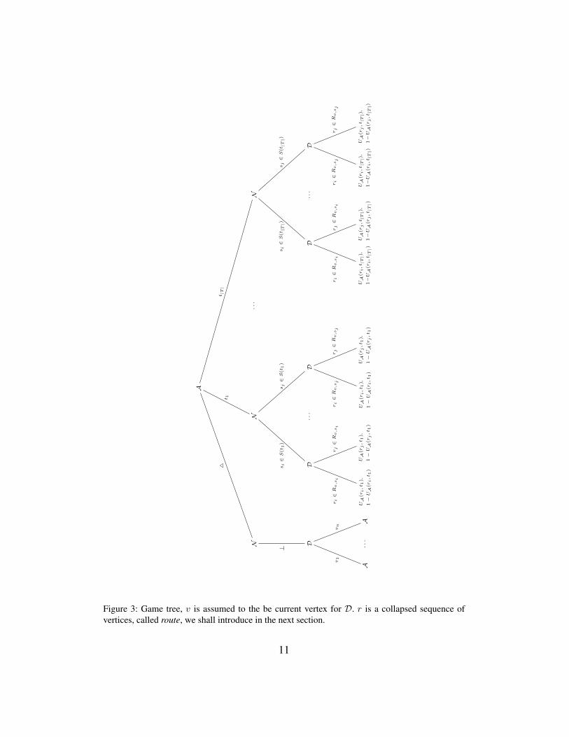
recurrent subgames. A portion of the game is depicted in Figure 3. Such tree canbe read along the following steps.
• Root of the tree. A decides whether to wait for a turn (this action is denotedby the symbol4 since no target is under attack) or to attack a target ti ∈ T(this action is denoted by the label ti of the target to attack).
10
A
N D
A
v1
···
A
vn
⊥
4
N
D
UA
(ri,t 1
),
1−
UA
(ri,t 1
)
ri∈
Rv,s
i
UA
(rj,t 1
),
1−
UA
(rj,t 1
)
rj∈
Rv,s
i
si∈
S(t
1)
···
D
UA
(ri,t 1
),
1−
UA
(ri,t 1
)
ri∈
Rv,s
j
UA
(rj,t 1
),
1−
UA
(rj,t 1
)
rj∈
Rv,s
j
sj∈
S(t
1)
t 1
···
N
D
UA
(ri,t |
T|)
,
1−U
A(r
i,t |
T|)
ri∈
Rv,s
i
UA
(rj,t |
T|)
,
1−
UA
(rj,t |
T|)
rj∈
Rv,s
i
si∈
S(t
|T|)
···
D
UA
(ri,t |
T|)
,
1−U
A(r
i,t |
T|)
ri∈
Rv,s
j
UA
(rj,t |
T|)
,
1−
UA
(rj,t |
T|)
rj∈
Rv,s
j
sj∈
S(t
|T|)
t |T
|
Figure 3: Game tree, v is assumed to the be current vertex for D. r is a collapsed sequence ofvertices, called route, we shall introduce in the next section.
11

• Second level of the tree. N denotes the alarm system, represented by anature–type player. Its behavior is a priori specified by the conditional prob-ability mass function p which determines the generated signal given the at-tack performed by A. In particular, it is useful to distinguish between twocases:
(a) if no attack is present, then no signal will be generated under the as-sumption that p(⊥ | 4) = 1;
(b) if an attack on target ti is taking place, a signal s will be drawn fromS(ti) with probability p(s | ti) (recall that we assumed p(⊥ | ti) = 0).
• Third level of the tree.D observes the signal raised by the alarm system anddecides the next vertex to patrol among those adjacent to the current one(the current vertex is initially chosen by D).
• Fourth level of the tree and on. It is useful to distinguish between two cases:
(a) if no attack is present, then the tree of the subgame starting from hereis the same of the tree of the whole game, except for the position of Dthat may be different from the initial one;
(b) if an attack is taking place on target ti, then only D can act.
Such game tree can be decomposed in a number of finite recurrent subgamessuch that the best strategies of the agents in each subgame are independent fromthose in other subgames. This decomposition allows us to apply a divide et imperaapproach, simplifying the resolution of the problem of finding an equilibrium.More precisely, we denote with Γ one of these subgames. We define Γ as a gamesubtree that can be extracted from the tree of Figure 3 as follows. Given D’scurrent vertex v ∈ V , select a decision node for A and call it i. Then, extract thesubtree rooted in i discarding the branch corresponding to action ∆ (no attack)5.
5Rigorously speaking, our definition of subgame is not compliant with the definition providedin game theory [30], which requires that all the actions of a node belong to the same subgame (andtherefore we could not separate action ∆ from actions ti). However, we can slightly change thestructure of our game making our definition of subgame compliant with the one from game theory.More precisely, it is sufficient to split each node of A into two nodes: in the first A decides toattack a target or to wait for one turn, and in the second, conditioned to the fact that A decided toattack,A decides which target to attack. This way, the subtree whose root is the second node ofAis a subgame compliant with game theory. It can be easily observed that this change to the gametree structure does not affect the behaviour of the agents.
12

Intuitively, such subgame models the players interaction when the Defender is insome given vertex v and the Attacker will perform an attack. As a consequence,each Γ obtained in such way is finite (once an attack on t started, the maximumlength of the game is d(t)). Moreover, the set of different Γs we can extract isfinite since we have one subgame for each possible current vertex for D, as aconsequence we can extract at most |V | different subgames. Notice that, due tothe infinite horizon, each subgame can recur an infinite number of times along thegame tree. However, being such repetitions independent and the game zero–sum,we only need to solve one subgame to obtain the optimal strategy to be appliedin each of its repetitions. In other words, when assuming that an attack will beperformed, the agents’ strategies can be split in a number of independent strategiessolely depending on the current position of the Defender. The reason why wediscarded the branch corresponding to action ∆ in each subgame is that we seekto deal with such complementary case exploiting a simple backward inductionapproach as explained in the following.
First, we call Signal Response Game from v the subgame Γ defined as aboveand characterized by a vertex v representing the current vertex of D (for brevity,we shall use SRG–v). In an SRG–v, the goal of D is to find the best strategy start-ing from vertex v to respond to any alarm signal. All the SRG–vs are independentone each other and thus the best strategy in each subgame does not depend onthe strategies of the other subgames. The intuition is that the best strategies in anSRG–v does not depend on the vertices visited by D before the attack. Given anSRG–v, we denote by σDv,s the strategy of D once observed signal s, by σDv thestrategy profile σDv = (σDv,s1 . . . , σ
Dv,sm) of D, and by σAv the strategy of A. Let us
notice that in an SRG–v, given a signal s,D is the only agent that plays and there-fore each sequence of moves between vertices of D in the tree can be collapsed ina single action. Thus, SRG–v is essentially a two–level game in which A decidesthe target to attack and D decides the sequence of moves to visit the targets.
Then, according to classical backward induction arguments [30], once we havefound the best strategies of each SRG–v, we can substitute the subgames with theagents’ equilibrium utilities and then we can find the best strategy of D for pa-trolling the vertices whenever no alarm signal has been raised and the best strategyof attack for A. We call this last problem Patrolling Game (for conciseness, weshall use PG). We denote by σD and σA the strategies of D and A respectively inthe PG.
13

2.2. The computational questions we poseIn the present paper, we focus on some questions whose answers play a funda-
mental role in the design of the best algorithms to find an equilibrium of our game.More precisely, we investigate the computational complexity of the following fourproblems. The first problem concerns the PG.
Question 1 Which is the best patrolling strategy for D maximizing its expectedutility?
The other three questions concern SRG–v. For the sake of simplicity, we focuson the case in which there is only one signal s, we shall show that it is possible toscale linearly in the number of signals.
Question 2 Given a starting vertex v and a signal s, is there any strategy of Dthat allows D to visit all the targets in T (s), each within its deadline?
Question 3 Given a starting vertex v and a signal s, is there any pure strategy ofD giving D an expected utility of at least k?
Question 4 Given a starting vertex v and a signal s, is there any mixed strategyof D giving D an expected utility of at least k?
In the following, we shall take a bottom–up approach answering the abovequestions starting from the last three and then dealing with the first one at thewhole–game level.
3. Signal response game on arbitrary graphs
In this section we show how to deal with an SRG–v on arbitrary graphs.Specifically, in Section 3.1 we prove the hardness of the problem, analyzing itscomputational complexity. Then, in Section 3.2 and in Section 3.3 we proposetwo algorithms, the first based on dynamic programming (breadth–first search)while the second adopts a branch and bound (depth–first search) paradigm. Fur-thermore, we provide a variation for each algorithm, approximating the optimalsolution.
14

3.1. Complexity resultsIn this section we analyse SRG–v from a computational point of view. We
initially observe that each SRG–v is characterized by |T | actions available to A,each corresponding to a target t, and by O(|V |maxtd(t)) decision nodes of D.The portion of game tree played by D can be safely reduced by observing thatD will move between any two targets along the minimum path. This allows usto discard from the tree all the decision nodes where D occupies a non–targetvertex. However, this reduction keeps the size of the game tree exponential inthe parameters of the game, specifically O(|T ||T |).6 The exponential size of thegame tree does not constitute a proof that finding the equilibrium strategies of anSRG–v requires exponential time in the parameters of the game because it doesnot exclude the existence of some compact representation of D’s strategies, e.g.,Markovian strategies. Indeed such representation should be polynomially upperbounded in the parameters of the game and therefore they would allow the designof a polynomial–time algorithm to find an equilibrium. We show below that it isunlikely that such a representation exists in arbitrary graphs, while it exists forspecial topologies as we shall discuss later.
We denote by gv the expected utility of A from SRG–v and therefore the ex-pected utility of D is 1− gv. Then, we define the following problem.
Definition 1 (k–SRG–v) The decision problem k–SRG–v is defined as:INSTANCE: an instance of SRG–v;QUESTION: is there any σD such that gv ≤ k (when A plays its best response)?
Theorem 1 k–SRG–v is strongly NP–hard even when |S| = 1.
Proof. Let us consider the following reduction from HAMILTONIAN–PATH [31].Given an instance of HAMILTONIAN–PATH GH = (VH , EH), we build an in-stance for k–SRG–v as:
• V = VH ∪ v;
• E = EH ∪ (v, h),∀h ∈ VH;
• T = VH ;
• d(t) = |VH |;
6A more accurate bound is O(|T |min|T |,maxtd(t)).
15

• π(t) ∈ (0, 1], for all t ∈ T (any value);
• S = s1;
• T (s1) = T ;
• p(s1 | t) = 1, for all t ∈ T ;
• k = 0.
If gs ≤ 0, then there must exist a path starting from v and visiting all the targetsin T by d = |VH |. Given the penetration times assigned in the above constructionand recalling that edge costs are unitary, the path must visit each target exactlyonce. Therefore, since T = VH , the game’s value is less than or equal to zero ifand only if GH admits a Hamiltonian path. This concludes the proof.
Notice that the problem of assessing the membership of k–SRG–v to NPis left open and it strictly depends on the size of the support of the strategy ofσDv . That is, if any strategy σDv has a polynomially upper bounded support, thenk–SRG–v is in NP . We conjecture it is not and therefore there can be optimalstrategies in which an exponential number of actions are played with strictly pos-itive probability. Furthermore, the above result shows that with arbitrary graphs:
• answering to Question 1 is FNP–hard,
• answering to Questions 2, 3, 4 is NP–hard.
As a consequence a polynomial–time algorithm solving those problems is unlikelyto exist. In particular, the above proof shows that we cannot produce a compactrepresentation (a.k.a. information lossless abstractions) of the space of strategiesof D that is smaller than O(2|T (s)|), unless there is an algorithm better than thebest–known algorithm for HAMILTONIAN–PATH. This is due to the fact thatthe best pure maxmin strategy can be found in linear time in the number of thepure strategies and the above proof shows that it cannot be done in a time less thanO(2|T (s)|). More generally, no polynomially bounded representation of the spaceof the strategies can exist, unless P = NP .
Although we can deal only with exponentially large representations of D’sstrategies, we focus on the problem of finding the most efficient representation.Initially, we provide the following definitions.
Definition 2 (Route) Given a starting vertex v and a signal s, a route (over thetargets) r is a generic sequence of targets of T (s) such that:
16

• r starts from v,
• each target t ∈ T (s) occurs at most once in r (but some targets may notoccur),
• r(i) is the i–th visited target in r (in addition, r(0) = v).
Among all the possible routes we restrict our attention on a special class of routesthat we call covering and are defined as follows.
Definition 3 (Covering Route) Given a starting vertex v and a signal s, a router is covering when, denoted by Ar(r(i)) =
∑i−1h=0 ω
∗r(h),r(h+1) the time needed by
D to visit target t = r(i) ∈ T (s) starting from r(0) = v and moving alongthe shortest path between each pair of consecutive targets in r, for every target toccurring in r it holds Ar(r(i)) ≤ d(r(i)) (i.e., all the targets are visited withintheir penetration times).
With a slight abuse of notation, we denote by T (r) the set of targets coveredby r and we denote by c(r) the total temporal cost of r, i.e., c(r) = Ar(r(|T (r)|)).Notice that in the worst case the number of covering routes is O(|T (s)||T (s)|), butcomputing all of them may be unnecessary since some covering routes will neverbe played by D due to strategy domination and therefore they can be safely dis-carded [32]. More precisely, we introduce the following two forms of dominance.
Definition 4 (Intra–Set Dominance) Given a starting vertex v, a signal s andtwo different covering routes r, r′ such that T (r) = T (r′), if c(r) ≤ c(r′) then rdominates r′.
Definition 5 (Inter–Set Dominance) Given a starting vertex v, a signal s andtwo different covering routes r, r′, if T (r) ⊃ T (r′) then r dominates r′.
Furthermore, it is convenient to introduce the concept of covering set, whichis strictly related to the concept of covering route. It is defined as follows.
Definition 6 (Covering Set) Given a starting vertex v and a signal s, a coveringset Q is a subset of targets T (s) such that there exists a covering route r withT (r) = Q.
Let us focus on Definition 4. It suggests that we can safely use only one routeper covering set. Covering sets suffice for describing all the outcomes of the game,since the agents’ payoffs depend only on the fact that A attacks a target t that is
17

covered byD or not, and in the worst case areO(2|T (s)|), with a remarkable reduc-tion of the search space w.r.t. O(|T (s)||T (s)|). However, any algorithm restrictingon covering sets should be able to determine whether or not a set of targets is acovering one. Unfortunately, this problem is hard too.
Definition 7 (COV–SET) The decision problem COV–SET is defined as:INSTANCE: an instance of SRG–v with a target set T ;QUESTION: is T a covering set for some covering route r?
By trivially adapting the same reduction for Theorem 1 we can state the fol-lowing theorem.
Theorem 2 COV–SET is NP–complete.
Therefore, computing a covering route for a given set of targets (or decidingthat no covering route exists) is not doable in polynomial time unless P = NP .This shows that, while covering sets suffice for defining the payoffs of the gameand therefore the size of payoffs matrix can be bounded by the number of cover-ing sets, in practice we also need covering routes to certificate that a given subsetof targets is covering. Thus, we need to work with covering routes, but we justneed the routes corresponding to the covering sets, limiting the number of cover-ing routes that are useful for the game to the number of covering sets. In addition,Theorem 2 suggests that no algorithm for COV–SET can have complexity betterthan O(2|T (s)|) unless there exists a better algorithm for HAMILTONIAN–PATHthan the best algorithm known in the literature. This seems to suggest that enu-merating all the possible subsets of targets (corresponding to all the potential cov-ering sets) and, for each of them, checking whether or not it is covering requiresa complexity worse than O(2|T (s)|). Surprisingly, we show in the next section thatthere is an algorithm with complexity O(2|T (s)|) (neglecting polynomial terms)to enumerate all and only the covering sets and, for each of them, one coveringroute. Therefore, the complexity of our algorithm matches (neglecting polynomialterms) the complexity of the best–known algorithm for HAMILTONIAN–PATH.
Let us focus on Definition 5. Inter–Set dominance can be leveraged to intro-duce the concept of maximal covering sets which could enable a further reductionin the set of actions available to D.
Definition 8 (MAXIMAL COV–SET) Given a covering setQ (whereQ = T (r)for some r), we say that Q is maximal if there is no route r′ such that Q ⊂ T (r′).
18

Furthermore, we say that r such that T (r) = Q is a maximal covering route. Inthe best case, when there is a route covering all the targets, the number of maximalcovering sets is 1, while the number of covering sets (including the non–maximalones) is 2|T (s)|. Thus, considering only maximal covering sets allows an exponen-tial reduction of the payoffs matrix. In the worst case, when all the possible subsetscomposed of |T (s)|/2 targets are maximal covering sets, the number of maximalcovering sets is O(2|T (s)|−2), while the number of covering sets is O(2|T (s)|−1), al-lowing a reduction of the payoffs matrix by a factor of 2. Furthermore, if we knewa priori that Q is a maximal covering set, we could avoid searching for coveringroutes for any set of targets that strictly contains Q. When designing an algorithmto solve this problem, Definition 5 could then be exploited to introduce some kindof pruning technique to save average compute time. However, the following resultshows that deciding if a covering set is maximal is hard.
Definition 9 (MAX–COV–SET) The decision problem MAX–COV–SET is de-fined as:INSTANCE: an instance of SRG–v with a target set T and a covering set T ′ ⊂ T ;QUESTION: is T ′ maximal?
Theorem 3 There is no polynomial–time algorithm for MAX–COV–SET unlessP = NP .
Proof. Assume for simplicity that S = s1 and that T (s1) = T . Initially, weobserve that MAX–COV–SET is in co–NP . Indeed, any covering route r suchthat T (r) ⊃ T ′ is a NO certificate for MAX–COV–SET, placing it in co–NP .(Notice that, trivially, any covering route has length bounded by O(|T |2); also,notice that due to Theorem 2, having a covering set would not suffice given that wecannot verify in polynomial time whether it is actually covering unless P = NP .)
Let us suppose we have a polynomial–time algorithm for MAX–COV–SET,called A. Then (since P ⊆ NP ∩ co–NP) we have a polynomial algorithm forthe complement problem, i.e., deciding whether all the covering routes for T ′ aredominated. Let us consider the following algorithm: given an instance for COV–SET specified by graph G = (V,E), a set of target T with penetration times d,and a starting vertex v:
1. assign to targets in T a lexicographic order t1, t2, . . . , t|T |;
2. for every t ∈ T , verify if t is a covering set in O(|T |) time by compar-ing ω∗v,t and d(t); if at least one is not a covering set, then output NO andterminate; otherwise set T = t1 and k = 2;
19

3. apply algorithm A on the following instance: graph G = (V,E), target setT∪tk, d (where d is d restricted to T∪tk), start vertex v, and coveringset T ;
4. if A’s output is YES (that is, T is not maximal) then set T = T ∪ tk,k = k + 1 and restart from step 3; if A’s output is NO and k = |T | thenoutput YES; if A’s output is NO and k < |T | then output NO;
Thus, the existence of A would imply the existence of a polynomial algorithm forCOV–SET which (under P 6= NP) would contradict Theorem 2. This concludesthe proof.
Nevertheless, we show hereafter that there exists an algorithm enumeratingall and only the maximal covering sets and one route for each of them (whichpotentially leads to an exponential reduction of the time needed for solving thelinear program) with only an additional polynomial cost w.r.t. the enumeration ofall the covering sets. Therefore, neglecting polynomial terms, our algorithm has acomplexity of O(2|T (s)|).
Finally, we focus on the complexity of approximating the best solution in anSRG–v. When D restricts its strategies to be pure, the problem is clearly not ap-proximable in polynomial time even when the approximation ratio depends on|T (s)|. The basic intuition is that, if a game instance admits the maximal coveringroute that covers all the targets and the value of all the targets is 1, then eitherthe maximal covering route is played returning a utility of 1 to D or any otherroute is played returning a utility of 0, but no polynomial–time algorithm can findthe maximal covering route covering all the targets, unless P = NP . On theother hand, it is interesting to investigate the case in which no restriction to purestrategies is present. We show that the problem keeps being hard.
Theorem 4 The optimization version of k–SRG–v, say OPT–SRG–v, is APX–hard even in the restricted case in which the graph is metric, there is only onesignal s, all targets t ∈ T (s) have the same penetration time d(t), and there is themaximal covering route covering all the targets.
Proof. We produce an approximation–preserving reduction from TSP(1,2) that isknown to beAPX–hard [33]. For the sake of clarity, we divide the proof in steps.
TSP(1,2) instance. An instance of undirected TSP(1,2) is defined as follows:
• a set of vertices VTSP ,
• a set of edges composed of an edge per pair of vertices,
20

• a symmetric matrix CTSP of weights, whose values can be 1 or 2, each as-sociated with an edge and representing the cost of the shortest path betweenthe corresponding pair of vertices.
The goal is to find the minimum cost tour. Let us denote by OPTSOLTSP andOPTTSP the optimal solution of TSP(1,2) and its cost, respectively. Further-more, let us denote by APXSOLTSP and APXTSP an approximate solution ofTSP(1,2) and its cost, respectively. It is known that there is no polynomial–timeapproximation algorithm with APXTSP/OPTAPX < α for some α > 1, unlessP = NP [33].
Reduction. We map an instance of TSP(1,2) to a specific instance of SRG–vas follows:
• there is only one signal s,
• T (s) = VTSP ,
• w∗t,t′ = CTSP (t, t′), for every t, t′ ∈ T (s),
• π(t) = 1, for every t ∈ T (s),
• w∗v,t = 1, for every t ∈ T (s),
• d(t) =
OPTTSP if OPTTSP = |VTSP |OPTTSP − 1 if OPTTSP > |VTSP |
, for every t ∈ T (s).
In this reduction, we use the value ofOPTTSP even if there is no polynomial–timealgorithm solving exactly TSP(1,2), unless P = NP . We show below that withan additional polynomial–time effort we can deal with the lack of knowledge ofOPTTSP .
OPT–SRG–v optimal solution. By construction of the SRG–v instance, there isa covering route starting from v and visiting all the targets t ∈ T (s), each within itspenetration time. This route has a cost of exactly d(t) and it is 〈v, t1, . . . , t|T (s)|〉,where 〈t1, . . . , t|T (s)|, t1〉 corresponds to OPTSOLTSP with the constraint thatw∗t|T (s)|,t1
= 2 if OPTTSP > |VTSP | (essentially, we transform the tour in a pathby discarding one of the edges with the largest cost). Therefore, the optimal so-lution of SRG–v, say OPTSOLSRG, prescribes to play the maximal route withprobability one and the optimal value, say OPTSRG, is 1.
OPT–SRG–v approximation. Let us denote by APXSOLSRG and APXSRG
an approximate solution of OPT–SRG–v and its value, respectively. We assume
21

there is a polynomial–time approximation algorithm with APXSRG/OPTSRG ≥β where β ∈ (0, 1). Let us notice that APXSOLSRG prescribes to play a polyno-mially upper bounded number of covering routes with strictly positive probability.We introduce a lemma that characterizes such covering routes.
Lemma 5 The longest covering route played with strictly positive probability inAPXSOLSRG visits at least β|T (s)| targets.
Proof. Assume by contradiction that the longest route visits β|T (s)|−1 targets.The best case in terms of maximization of the value of OPT–SRG–v is, due toreasons of symmetry (all the targets have the same value), when there is a setof |T (s)| covering routes of length β|T (s)| − 1 such that each target is visitedexactly by β|T (s)| − 1 routes. When these routes are available, the best strategyis to randomize uniformly over the routes. The probability that a target is coveredis β − 1
|T (s)| and therefore the value of APXSRG is β − 1|T (s)| . This leads to a
contradiction, since the algorithm would provide an approximation strictly smallerthan β.
TSP(1,2) approximation from OPT–SRG–v approximation. We use the abovelemma to show that we can build a (3−2β)–approximation for TSP(1,2) from a β–approximation of OPT–SRG–v. Given an APXSOLSRG, we extract the longestcovering route played with strictly positive probability, say 〈v, t1, . . . , tβ|T (s)|〉.The route has a cost of at most d(t), it would not cover β|T (s)| targets other-wise. Any tour 〈t1, . . . , tβ|T (s)|, tβ|T (s)|+1, . . . , t|T (s)|, t1〉 has a cost not larger thand(t) − 1 + 2(1 − β)|T (s)| = OPTTSP − 1 + 2(1 − β)|VTSP | (under the worstcase in which all the edges in 〈tβ|T (s)|, tβ|T (s)|+1, . . . , t|T (s)|, t1〉 have a cost of 2).Given that OPTTSP ≥ |VTSP |, we have that such a tour has a cost not largerthan OPTTSP − 1 + 2(1 − β)|VTSP | ≤ OPTTSP (3 − 2β). Therefore, the touris a (3 − 2β)–approximation for TSP(1,2). Since TSP(1,2) is not approximablein polynomial time for any approximation ratio smaller than α, we have the con-straint that 3 − 2β ≥ α, and therefore that β ≤ 3−α
2. Since α > 1, we have that
3−α2< 1 and therefore that there is no polynomial–time approximation algorithm
for OPT–SRG–v when β ∈ (3−α2, 1), unless P = NP .
OPTTSP oracle. In order to deal with the fact that we do not know OPTTSP ,we can execute the approximation algorithm for OPT–SRG–v using a guess overOPTTSP . More precisely, we execute the approximation algorithm for every valuein |VTSP |, . . . , 2|VTSP | and we return the best approximation found for TSP(1,2).Given thatOPTTSP ∈ |VTSP |, . . . , 2|VTSP |, there is an execution of the approx-imation algorithm that uses the correct guess.
22

We report some remarks to the above theorem.
Remark 1 The above result does not exclude the existence of constant–ratio ap-proximation algorithms for OPT–SRG–v. We conjecture that it is unlikely. OPT–SRG–v presents similarities with the (metric) DEADLINE–TSP, where the goalis to find the longest path of vertices each traversed before its deadline. TheDEADLINE–TSP does not admit any constant–ratio approximation algorithm [34]and the best–known approximation algorithm has logarithmic approximation ra-tio [35]. The following observations can be produced about the relationships be-tween OPT–SRG–v and DEADLINE–TSP:
• when the maximal route covering all the targets in the OPT–SRG–v exists,the optimal solution of the OPT–SRG–v is also optimal for the DEADLINE–TSP applied to the same graph;
• when the maximal route covering all the targets in the OPT–SRG–v doesnot exist, the optimal solutions of the two problems are different, even whenwe restrict us to pure–strategy solutions for the OPT–SRG–v;
• approximating the optimal solution of the DEADLINE–TSP does not givea direct technique to approximate OPT–SRG–v, since we should enumerateall the subsets of targets and for each subset of targets we would need toexecute the approximation of the DEADLINE–TSP, but this would requireexponential time. We notice in addition that even the total number of setsof targets with logarithmic size is not polynomial, being Ω(2log2(|T |)), andtherefore any algorithm enumerating them would require exponential time;
• when the optimal solution of the OPT–SRG–v is randomized, examples ofoptimal solutions in which maximal covering routes are not played can beproduced, showing that at the optimum it is not strictly necessary to playmaximal covering routes, but even approximations suffice.
Remark 2 If it is possible to map DEADLINE–TSP instances to OPT–SRG–vinstances where the maximal covering route covering all the targets exists, thenit trivially follows that OPT–SRG–v does not admit any constant–approximationratio. We were not able to find such a mapping and we conjecture that, if there isan approximation–preserving reduction from DEADLINE–TSP to OPT–SRG–v,then we cannot restrict to such instances. The study of instances of OPT–SRG–vwhere mixed strategies may be optimal make the treatment very challenging.
23

3.2. Dynamic–programming algorithmWe start by presenting two algorithms. The first one is exact, while the sec-
ond one is an approximation algorithm. Both algorithms are based on a dynamicprogramming approach.
3.2.1. Exact algorithmHere we provide an algorithm based on the dynamic programming paradigm
returning the set of strategies available to D when it is in v and receives a signals. The algorithm we present in this section enumerates all the covering sets and,for each of them, it returns also the corresponding covering route. Initially, weobserve that we can safely restrict our attention to a specific class of covering sets,that we call proper, defined as follows.
Definition 10 (Proper Covering Set) Given a starting vertex v and a signal s, acovering set Q is proper if there is a route r such that, once walked (along theshortest paths) over graph G, it does not traverse any target t ∈ T (s) \ T (r).
While in the worst case the number of proper covering sets is equal to the num-ber of covering sets (consider, for example, fully connected graphs with unitaryedge costs) in realistic scenarios we expect that the number of proper coveringsets is much smaller than the number of covering sets. As we show in Section 5,restricting to proper covering sets makes the complexity of our algorithm poly-nomial with respect to some special topologies: differently from the number ofcovering sets, the number of proper covering sets is polynomially upper bounded.Hereafter we provide the description of the algorithm.
Let us denote Ckv,t a collection of proper covering sets, where each set in this
collection is denoted as Qkv,t. The proper covering set Qk
v,t has cardinality k andadmits a covering route r whose starting vertex is v and whose last covered targetis t. Each Qk
v,t is associated with a cost c(Qkv,t) representing the temporal cost
of the shortest covering route for Qkv,t that specifies t as the k–th target to visit.
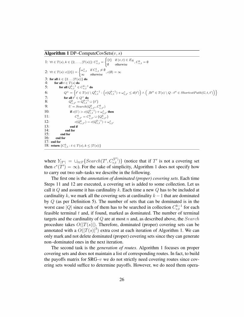
Upon this basic structure, our algorithm iteratively computes proper covering setscollections and costs for increasing cardinalities, that is from k = 1 possibly up tok = |T (s)| including one target at each iteration. Using a dynamic programmingapproach, we assume to have solved up to cardinality k − 1 and we specify howto complete the task for cardinality k. Detailed steps are reported in Algorithm 1,while in the following we provide an intuitive description. Given Qk−1
v,t , we cancompute a set of targets Q+ (Line 6) that is a subset of T (s) such that for eachtarget t′ ∈ Q+ the following properties hold:
24
• t′ 6∈ Qk−1v,t ,
• if t′ is appended to the shortest covering route for Qk−1v,t , it will be visited
before d(t′),
• the shortest path between t and t′ does not traverse any target t′′ ∈ T (s) \Qk−1v,t .
Function ShortestPath(G, t, t′) returns the shortest path on G between t andt′. For efficiency, we calculate (in polynomial time) all the shortest paths offline bymeans of the Floyd–Warshall algorithm [36]. IfQ+ is not empty, for each t′ ∈ Q+,we extend Qk−1
v,t (Step 8) by including it and naming the resulting covering set asQkv,t′ since it has cardinality k and we know it admits a covering route with last
vertex t′. Such route can be obtained by appending t′ to the covering route forQk−1v,t and has cost c(Qk−1
v,t ) + ω∗t,t′ . This value is assumed to be the cost of theextended proper covering set.—In Step 9, we make use of a procedure calledSearch(Q,C) where Q is a covering set and C is a collection of covering sets.The procedure outputs Q if Q ∈ C and ∅ otherwise. We adopted an efficientimplementation of such procedure which can run in O(|T (s)|). More precisely,we represent a covering set Q as a binary vector of length |T (s)| where the i–thcomponent is set to 1 if target ti ∈ Q and 0 otherwise. A collection of coveringsets C can then be represented as a binary tree with depth |T (s)|. The membershipof a covering set Q to collection C is represented with a branch of the tree in sucha way that if ti ∈ Q then we have a left edge at depth i − 1 on such branch. Wecan easily determine if Q ∈ C by checking if traversing a left (right) edge in thetree each time we read a 1 (0) in Q’s binary vector we reach a leaf node at depth|T (s)|. The insertion of a new covering set in the collection can be done in thesame way by traversing existing edges and expanding the tree where necessary.—If such extended proper covering set is not present in collection Ck
v,t′ or is alreadypresent with a higher cost (Step 10), then collection and cost are updated (Steps 11and 12). After the iteration for cardinality k is completed, for each proper coveringset Q in collection Ck
v,t, c(Q) represents the temporal cost of the shortest coveringroute with t as last target.
After Algorithm 1 completed its execution, for any arbitrary T ′ ⊆ T we caneasily obtain the temporal cost of its shortest covering route as
c∗(T ′) = minQ∈Y|T ′|
c(Q)
25
Algorithm 1 DP–ComputeCovSets(v, s)
1: ∀t ∈ T (s), k ∈ 2, . . . , |T (s)|: C1v,t =
t if (v, t) ∈ ER
∅ otherwise, Ck
v,t = ∅
2: ∀t ∈ T (s): c(t) =ω∗v,t if C1
v,t 6= ∅∞ otherwise
, c(∅) =∞
3: for all k ∈ 2 . . . |T (s)| do4: for all t ∈ T (s) do5: for all Qk−1
v,t ∈ Ck−1v,t do
6: Q+ =t′ ∈ T (s) \Qk−1
v,t :(c(Qk−1
v,t ) + ω∗t,t′ ≤ d(t
′))∧(6 ∃t′′ ∈ T (s) \Q : t′′ ∈ ShortestPath(G, t, t′)
)7: for all t′ ∈ Q+ do8: Qk
v,t′ = Qk−1v,t ∪ t′
9: U = Search(Qkv,t′ , C
kv,t′ )
10: if c(U) > c(Qk−1v,t ) + ω∗
t,t′ then11: Ck
v,t′ = Ckv,t′ ∪ Q
kv,t′
12: c(Qkv,t′ ) = c(Qk−1
v,t ) + ω∗t,t′
13: end if14: end for15: end for16: end for17: end for18: return Ck
v,t : t ∈ T (s), k ≤ |T (s)|
where Y|T ′| = ∪t∈TSearch(T ′, C|T ′|v,t ) (notice that if T ′ is not a covering set
then c∗(T ′) = ∞). For the sake of simplicity, Algorithm 1 does not specify howto carry out two sub–tasks we describe in the following.
The first one is the annotation of dominated (proper) covering sets. Each timeSteps 11 and 12 are executed, a covering set is added to some collection. Let uscall it Q and assume it has cardinality k. Each time a new Q has to be included atcardinality k, we mark all the covering sets at cardinality k−1 that are dominatedby Q (as per Definition 5). The number of sets that can be dominated is in theworst case |Q| since each of them has to be searched in collection Ck−1
v,t for eachfeasible terminal t and, if found, marked as dominated. The number of terminaltargets and the cardinality of Q are at most n and, as described above, the Searchprocedure takes O(|T (s)|). Therefore, dominated (proper) covering sets can beannotated with a O(|T (s)|3) extra cost at each iteration of Algorithm 1. We canonly mark and not delete dominated (proper) covering sets since they can generatenon–dominated ones in the next iteration.
The second task is the generation of routes. Algorithm 1 focuses on propercovering sets and does not maintain a list of corresponding routes. In fact, to buildthe payoffs matrix for SRG–v we do not strictly need covering routes since cov-ering sets would suffice to determine payoffs. However, we do need them opera-
26

tively sinceD should know in which order targets have to be covered to physicallyplay an action. This task can be accomplished by maintaining an additional list ofroutes where each route is obtained by appending terminal vertex t′ to the routestored for Qk−1
v,t when set Qk−1v,t ∪ t′ is included in its corresponding collection.
At the end of the algorithm only routes that correspond to non–dominated (proper)covering sets are returned. Maintaining such a list introduces a O(1) cost.
Theorem 6 The worst–case complexity of Algorithm 1 is O(|T (s)|22|T (s)|) sinceit has to compute proper covering sets up to cardinality |T (s)|. With annotationsof dominances and routes generation the whole algorithm yields a worst–casecomplexity of O(|T (s)|52|T (s)|).
3.2.2. Approximation algorithmThe dynamic programming algorithm presented in the previous section can-
not be directly adopted to approximate the maximal covering routes. We noticethat even in the case we introduce a logarithmic upper bound over the size ofthe covering sets generated by Algorithm 1, we could obtain a number of routesthat is O(2log2(|T (s)|)), and therefore exponential. Thus, our goal is to design apolynomial–time algorithm that generates a polynomial number of good coveringroutes. We observe that if we have a total order over the vertices and we workover the complete graph of the targets where each edge corresponds to the short-est path, we can find in polynomial time the maximal covering routes subject tothe constraint that, given any pair of targets t, t′ in a route, t can precede t′ in theroute only if t precedes t′ in the order. We call monotonic a route satisfying a giventotal order. Algorithm 2 returns the maximal monotonic covering routes when thetotal order is lexicographic (trivially, in order to change the order, it is sufficientto re–label the targets).
Algorithm 2 is based on dynamic programming and works as follows. R(k, l)is a matrix storing in each cell one route, while L(k, l) is a matrix storing ineach cell the maximum lateness of the corresponding route, where the latenessassociated with a target t is the difference between the (first) arrival time at talong r and d(t) and the maximum lateness of the route is the maximum latenessof the targets covered by the route. The route stored in R(k, l) is the one with theminimum lateness among all the monotonic ones covering l targets where tk is thefirst visited target. Thus, basically, when l = 1, R(k, l) contains the route 〈v, tk〉,while, when l > 1, R(k, l) is defined appending to R(k, 1) the best (in terms ofminimizing the maximum lateness) route R(k′, l− 1) for every k′ > k, in order to
27
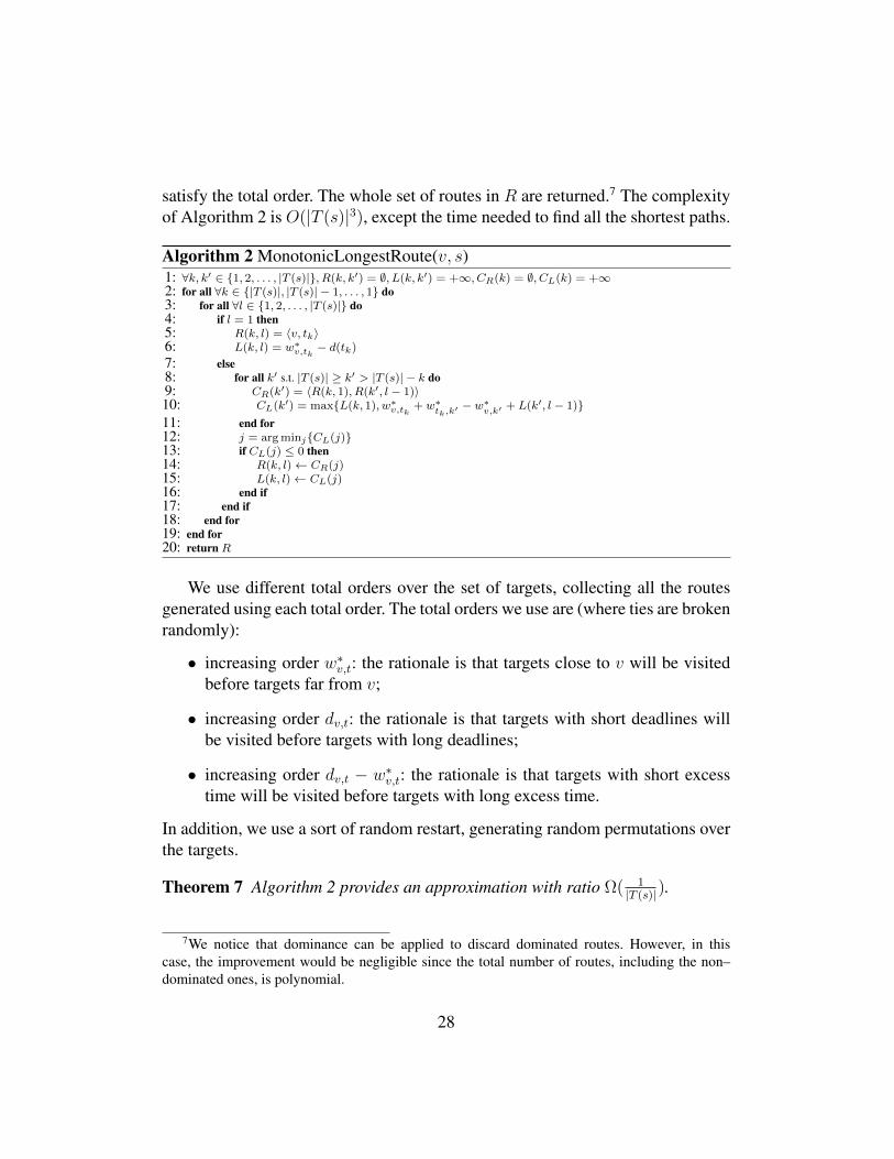
satisfy the total order. The whole set of routes in R are returned.7 The complexityof Algorithm 2 is O(|T (s)|3), except the time needed to find all the shortest paths.
Algorithm 2 MonotonicLongestRoute(v, s)1: ∀k, k′ ∈ 1, 2, . . . , |T (s)|, R(k, k′) = ∅, L(k, k′) = +∞, CR(k) = ∅, CL(k) = +∞2: for all ∀k ∈ |T (s)|, |T (s)| − 1, . . . , 1 do3: for all ∀l ∈ 1, 2, . . . , |T (s)| do4: if l = 1 then5: R(k, l) = 〈v, tk〉6: L(k, l) = w∗v,tk − d(tk)7: else8: for all k′ s.t. |T (s)| ≥ k′ > |T (s)| − k do9: CR(k′) = 〈R(k, 1), R(k′, l − 1)〉10: CL(k
′) = maxL(k, 1), w∗v,tk + w∗tk,k
′ − w∗v,k′ + L(k′, l − 1)11: end for12: j = argminjCL(j)13: if CL(j) ≤ 0 then14: R(k, l)← CR(j)15: L(k, l)← CL(j)16: end if17: end if18: end for19: end for20: return R
We use different total orders over the set of targets, collecting all the routesgenerated using each total order. The total orders we use are (where ties are brokenrandomly):
• increasing order w∗v,t: the rationale is that targets close to v will be visitedbefore targets far from v;
• increasing order dv,t: the rationale is that targets with short deadlines willbe visited before targets with long deadlines;
• increasing order dv,t − w∗v,t: the rationale is that targets with short excesstime will be visited before targets with long excess time.
In addition, we use a sort of random restart, generating random permutations overthe targets.
Theorem 7 Algorithm 2 provides an approximation with ratio Ω( 1|T (s)|).
7We notice that dominance can be applied to discard dominated routes. However, in thiscase, the improvement would be negligible since the total number of routes, including the non–dominated ones, is polynomial.
28

Proof sketch. The worst case for the approximation ratio of our algorithm occurswhen the covering route including all the targets exists and each covering routereturned by our heuristic algorithm visits only one target. In that case, the optimalexpected utility of D is 1. Our algorithm, in the worst case in which π(t) = 1 forevery target t, returns an approximation ratio Ω( 1
|T (s)|). It is straightforward to seethat, in other cases, the approximation ratio is larger.
3.3. Branch–and–bound algorithmsThe dynamic programming algorithm presented in the previous section essen-
tially implements a breadth–first search. In some specific situations, depth–firstsearch could outperform breadth–first search, e.g., when penetration times arerelaxed and good heuristics lead a depth–first search to find in a brief time themaximal covering route, avoiding to scan an exponential number of routes as thebreadth–first search would do. In this section, we adopt the branch–and–boundapproach to design both an exact algorithm and an approximation algorithm. Inparticular, in Section 3.3.1 we describe our exact algorithm, while in Section 3.3.2we present the approximation one.
3.3.1. Exact algorithmOur branch–and–bound algorithm (see Algorithm 3) is a tree–search based
algorithm working on the space of the covering routes and returning a set of cov-ering routes R. It works as follows.
Initial step. We exploit two global set variables, CLmin and CLmax initiallyset to empty (Steps 1–2 of Algorithm 3). These variables contain closed coveringroutes, namely covering routes which cannot be further expanded without violat-ing the penetration time of at least one target during the visit. CLmax contains thecovering routes returned by the algorithm (Step 8 of Algorithm 3), while CLminis used for pruning as discussed below. The update of CLmin and CLmax is drivenby Algorithm 5, as discussed below. Given a starting vertex v and a signal s, foreach target t ∈ T (s) such that w∗v,t ≤ d(t) we generate a covering route r withr(0) = v and r(1) = t (Steps 1–3 of Algorithm 3). Thus, D has at least onecovering route per target that can be covered in time from v. Notice that if, forsome t, such minimal route does not exist, then target t cannot be covered becausewe assume triangle inequality. This does not guarantee that A will attack t withfull probability since, depending on the values π, A could find more profitable torandomize over a different set of targets. The meaning of parameter ρ is describedbelow.
29

Algorithm 3 Branch–and–Bound(v, s, ρ)1: CLmax ← ∅2: CLmin ← ∅3: for all t ∈ T (s) do4: if w∗v,t ≤ d(t) then5: Tree–Search(dρ · |T (s)|e, 〈v, t〉)6: end if7: end for8: return CLmax
Route expansions. The subsequent steps essentially evolve on each branchaccording to a depth–first search with backtracking limited by ρ (Step 4 of Al-gorithm 3). The choice of ρ directly influences the behavior of the algorithm andconsequently its complexity. Each node in the search tree represents a route r builtso far starting from an initial route 〈v, t〉. At each iteration, route r is expanded byinserting a new target at a particular position. We denote with r+(q, p) the routeobtained by inserting target q after the p–th target in r. Notice that every expansionof r will preserve the relative order with which targets already present in r willbe visited. The collection of all the feasible expansions r+s (i.e., the ones that arecovering routes) is denoted by R+ and it is ordered according to a heuristic thatwe describe below. Algorithm 6, described below, is used to generate R+ (Step 1of Algorithm 4). In each open branch (i.e.,R+ 6= ∅), if the depth of the node in thetree is smaller or equal to dρ · |T (s)|e then backtracking is disabled (Steps 7–11 ofAlgorithm 4), while, if the depth is larger than such value, is enabled (Steps 5–6of Algorithm 4). This is equivalent to fix the relative order of the first (at most)dρ · |T (s)|e inserted targets in the current route. In this case, with ρ = 0 we do notrely on the heuristics at all, full backtracking is enabled, the tree is fully expandedand the returned R is complete, i.e., it contains all the non–dominated coveringroutes. Route r is repeatedly expanded in a greedy fashion until no insertion ispossible. As a result, Algorithm 4 generates at most |T (s)| covering routes.
Pruning. Algorithm 5 is in charge of updating CLmin and CLmax each timea route r cannot be expanded and, consequently, the associated branch must beclosed. We call CLmin the minimal set of closed routes. This means that a closedroute r belongs to CLmin only if CLmin does not already contain another r′ ⊆ r.Steps 1–6 of Algorithm 5 implement such condition: first, in Steps 2–3 any router′ such that r′ ⊇ r is removed from CLmin, then route r is inserted in CLmin.Routes in CLmin are used by Algorithm 6 in Steps 2 and 6 for pruning duringthe search. More precisely, a route r is not expanded with a target q at positionp if there exists a route r′ ∈ CLmin such that r′ ⊆ r+(q, p). This pruning rule
30

Algorithm 4 Tree–Search(k, r)1: R+ = r(1), r(2), . . . ← Expand(r)2: if R+ = ∅ then3: Close(r)4: else5: if k > 0 then6: Tree–Search(k − 1, r(1))7: else8: for all r+ ∈ R+ do9: Tree–Search(0, r+)
10: Close(r+)11: end for12: end if13: end if
is safe since by definition if r′ ∈ CLmin, then all the possible expansions of r′
are unfeasible and if r′ ⊆ r then r can be obtained by expanding from r′. Thispruning mechanism explains why once a route r is closed is always inserted inCLmin without checking the insertion against the presence in CLmin of a route r′′
such that r′′ ⊆ r. Indeed, if such route r′′ would be included in CLmin we wouldnot be in the position of closing r, having r being pruned before by Algorithm 6in Step 2 or Step 8.
We use CLmax to maintain a set of the generated maximal closed routes. Thismeans that a closed route r is inserted here only ifCLmax does not already containanother r′ such that r′ ⊇ r. This set keeps track of closed routes with maximumnumber of targets. Algorithm 5 maintains this set by inserting a closed route rin Step 12 only if no route r′ ⊇ r is already present in CLmax. Once the wholealgorithm terminates, CLmax contains the final solution.
Algorithm 5 Close(r)1: for all r′ ∈ CLmin do2: if r ⊆ r′ then3: CLmin = CLmin \ r′4: end if5: end for6: CLmin = CLmin ∪ r7: for all r′ ∈ CLmax do8: if r ⊆ r′ then9: return
10: end if11: end for12: CLmax = CLmax ∪ r
Heuristic function. A key component of this algorithm is the heuristic func-tion that drives the search. The heuristic function is defined as hr : T (s)\T (r)×
31

1 . . . |T (r)| → Z, where hr(t′, p) evaluates the cost of expanding r by insertingtarget t′ after the p–th target of r. The basic idea, inspired by [37], is to adopt aconservative approach, trying to preserve feasibility. Given a route r, let us definethe possible forward shift of r as the minimum temporal margin in r between thearrival at a target t and d(t):
PFS(r) = mint∈T (r)(d(t)− Ar(t))The extra mileage er(t′, p) for inserting target t′ after position p is the addi-
tional traveling cost to be paid:
er(t′, p) = (Ar(r(t
′)) + ω∗r(p),t′ + ω∗t′,r(p+1))− Ar(r(p+ 1))
The advance time that such insertion gets with respect to d(t′) is defined as:
ar(t′, p) = d(t′)− (Ar(r(p)) + ω∗r(p),t′)
Finally, hr(t′, p) is defined as:
hr(t′, p) = minar(t′, p); (PFS(r)− er(t′, p))
We partition the set T (s) in two sets Ttight and Tlarge where t ∈ Ttight if d(t) <δ · ω∗v,t and t ∈ Tlarge otherwise (δ ∈ R is a parameter). The previous inequalityis a non–binding choice we made to discriminate targets with a tight penetrationtime from those with a large one. Initially, we insert all the tight targets and onlysubsequently we insert the non–tight targets. We use the two sets according to thefollowing rules (see Algorithm 6):
• the insertion of a target belonging to Ttight is always preferred to the inser-tion of a target belonging to Tlarge, independently of the insertion position;
• insertions of t ∈ Ttight are ranked according to h considering first the inser-tion position and then the target;
• insertions of t ∈ Tlarge are ranked according to h considering first the targetand then the insertion position.
The rationale behind this rule is that targets with a tight penetration time shouldbe inserted first and at their best positions. On the other hand, targets with a largepenetration time can be covered later. Therefore, in this last case, it is less impor-tant which target to cover than when to cover it.
Theorem 8 Algorithm 3 with ρ = 0 is an exact algorithm and has an exponentialcomputational complexity since it builds a full tree of covering routes with worst–case size O(|T (s)||T (s)|).
32

Algorithm 6 Expand(r)1: if Ttight * T (r) then2: for all q ∈ Ttight \ T (r) do
Pq = p(1)q , p(2)q , . . . p
(b)q s.t. ∀i ∈ 1, . . . , b,
hr(q, p
(i)q ) ≥ hr(q, p(i+1)
q )
r+(q, p(i)q ) is a covering route
6 ∃v′ ∈ CLmin : r′ ⊆ r+(q, p(i)q )
3: end for4: Q = q(1), q(2), . . . , q(c) s.t. ∀i ∈ 1, . . . , c, hr(q(i), p(1)
q(i)) ≥ hr(q(i+1), p
(1)
q(i+1) )
5: R+ = r(1), r(2), . . . r(k) where
r(1) = r+(q(1), p
(1)
q(1))
· · · = · · ·r(k) = r+(q(c), p
(b)
q(c))
6: end if7: if Tlarge * T (r) then8: for all u ∈ Tlarge \ T (r) do
Qp = q(1)p , q(2)p , . . . q
(b)p s.t. ∀i ∈ 1, . . . , b,
hr(q
(i)p , p) ≥ hr(q(i+1)
p , p)
r+(q(i)p , p) is a covering route
6 ∃ r′ ∈ CLmin : r′ ⊆ r+(q(i)p , p)
9: end for10: P = p(1), p(2), . . . , p(c) s.t. ∀i ∈ 1, . . . , c, hr(q(1), p(i)
q(1)) ≥ hr(q(1), p(i+1)
q(1))
11: R+ = R+ ∪ r(k+1), r(k+2), . . . r(K) where
r(k+1) = r+(q
(1)p , p(1))
· · · = · · ·r(K) = r+(q
(b)p , p(c))
12: end if13: return R+
3.3.2. Approximation algorithmSince ρ determines the completness degree of the generated tree, we can ex-
ploit Algorithm 3 tuning ρ to obtain an approximation algorithm that is faster w.r.t.the exact one.
In fact, when ρ < 1 completeness is not guaranteed in favour of a less com-putational effort. In this case, the only guarantees that can be provided for eachcovering route r ∈ CLmax, once the algorithm terminates are:
• no other r′ ∈ CLmax dominates r;
• no other r′ /∈ CLmax such that r ⊆ r′ dominates r. Notice this does notprevent the existence of a route r′′ not returned by the algorithm that visitstargets T (r) in a different order and that dominates r.
When ρ is chosen as k|T (s)| (where k ∈ N is a parameter), the complexity of gen-
erating covering routes becomes polynomial in the size of the input. We can statethe following theorem, whose proof is analogous to that one of Theorem 7.
33

Theorem 9 Algorithm 4 with ρ = k|T (s)| provides an approximation with ra-
tio Ω( 1|T (s)|) and runs in O(|T (s)|3) given that heuristic hr can be computed in
O(|T (s)|2).
3.4. Solving SRG–vNow we can formulate the problem of computing the optimal signal–response
strategy forD. Let us denote with σDv,s(r) the probability with whichD plays router under signal s and with Rv,s the set of all the routes available to D generated bysome algorithm. We introduce function UA(r, t), representing the utility functionof A and defined as follows:
UA(r, t) =
π(t) if t 6∈ r0 otherwise
.
The best D strategy (i.e., the maxmin strategy) can be found by solving thefollowing linear mathematical programming problem:
min gv s.t.∑s∈S(t)
p(s | t)∑
r∈Rv,s
σDv,s(r)UA(r, t) ≤ gv ∀t ∈ T∑r∈Rv,s
σDv,s(r) = 1 ∀s ∈ S
σDv,s(r) ≥ 0 ∀r ∈ Rv,s, s ∈ SThe size of the mathematical program is composed of |T | + |S| constraints
(excluded ≥ 0 constraints) and O(|V ||S|maxv,s|Rv,s|) variables. This showsthat the hardness is due only to maxv,s|Rv,s|, which, in its turn, depends onlyon |T (s)|. We provide the following remark.
Remark 3 We observe that the discretization of the environment as a graph is asaccurate as the number of vertices is large, corresponding to reduce the size ofthe areas associated with each vertex, as well as to reduce the temporal intervalassociated with each turn of the game. Our algorithms show that increasing theaccuracy of the model in terms of number of vertices requires polynomial time.
4. SRG–v on special topologies
In this section, we focus on special topologies, showing in Section 4.1 thetopologies with which solving a SRG–v is computationally easy, those that arehard in Section 4.2, and the topologies for which the problem remains open inSection 4.3.
34

4.1. Easy topologiesIn this section, we show that, with some special topologies, there exists an
efficient algorithm to solve exactly the SRG–v.Let us consider a linear graph. An example is depicted in Figure 4. We state
the following theorem.
t1 t2 v t3 t4
Figure 4: Linear graph.
Theorem 10 There is a polynomial–time algorithm solving OPT–SRG–v with lin-ear graphs.
Proof. We show that Algorithm 1 requires polynomial time in generating all thepure strategies of D. The complexity of Algorithm 1, once applied to a giveninstance, depends on the number of proper covering sets (recall Definition 10).It can be shown that linear graphs have a polynomial number of proper coveringsets. Given a starting vertex v, any proper covering set Q can be characterized bytwo extreme targets of Q, the first being the farthest from v on the left of v (ifany, and v otherwise) and the second being the farthest from v on the right of v(if any, and v otherwise). For example, see Figure 4, given proper covering setQ = t1, t2, t3, the left extreme is t1 and the right extreme is t3. Therefore, thenumber of proper covering sets for each pair v, s is O(|T (s)|2). Since the actionsavailable to D are polynomially upper bounded, the time needed to compute themaxmin strategy is polynomial.
Let us consider a cycle graph. An example is depicted in Figure 5. We canstate the following theorem.
Theorem 11 There is a polynomial–time algorithm solving OPT–SRG–v with cy-cle graphs (perimeters).
Proof. The proof is analogous to that one of linear graphs. That is, each propercovering set can be characterized by two extremes: the left one and the right one.For example, see Figure 5, given proper covering set Q = t1, t2, t4, t5, t6, t7, theleft extreme is t4 and the right extreme is t2. As in linear graphs, the number ofproper covering sets in a cycle graph is O(|T (s)|2).
The above results can be generalized to the case of tree graphs where thenumber of leaves is fixed. We can state the following theorem.
35
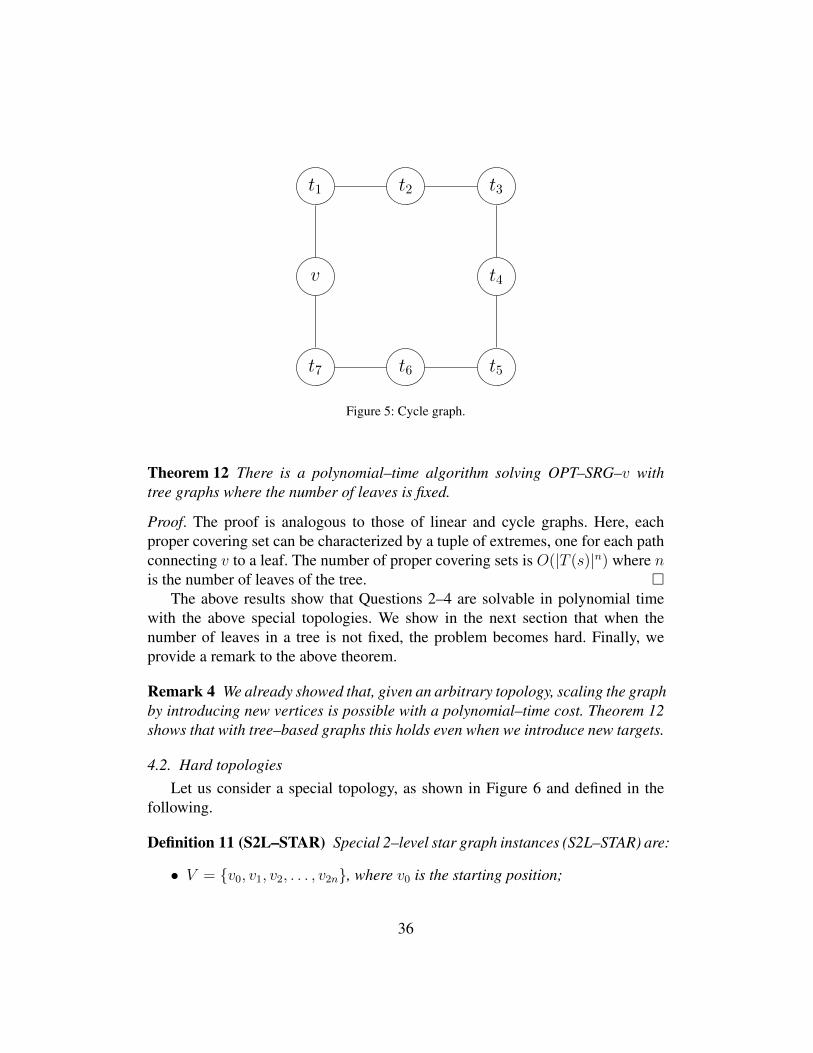
t1 t2 t3
t4
t5t6t7
v
Figure 5: Cycle graph.
Theorem 12 There is a polynomial–time algorithm solving OPT–SRG–v withtree graphs where the number of leaves is fixed.
Proof. The proof is analogous to those of linear and cycle graphs. Here, eachproper covering set can be characterized by a tuple of extremes, one for each pathconnecting v to a leaf. The number of proper covering sets is O(|T (s)|n) where nis the number of leaves of the tree.
The above results show that Questions 2–4 are solvable in polynomial timewith the above special topologies. We show in the next section that when thenumber of leaves in a tree is not fixed, the problem becomes hard. Finally, weprovide a remark to the above theorem.
Remark 4 We already showed that, given an arbitrary topology, scaling the graphby introducing new vertices is possible with a polynomial–time cost. Theorem 12shows that with tree–based graphs this holds even when we introduce new targets.
4.2. Hard topologiesLet us consider a special topology, as shown in Figure 6 and defined in the
following.
Definition 11 (S2L–STAR) Special 2–level star graph instances (S2L–STAR) are:
• V = v0, v1, v2, . . . , v2n, where v0 is the starting position;
36

• T = V \v0, where vertices vi with i ∈ 1, . . . , n are called inner targets,while vertices vi with i ∈ n+ 1, . . . , 2n are called outer targets;
• E = (v0, vi), (vi, vn+i) : ∀i ∈ 1, . . . , n and we call i–th branch thepair of edges ((v0, vi), (vi, vn+i));
• travel costs are c(v0, vi) = c(vi, vn+i) = γi for every i ∈ 1, . . . , n, whereγi ∈ N+;
• penetration times are, for i ∈ 1, . . . , n, d(t) =
6H − 3γi t = vi
10H − 2γi, t = vn+i,
where H =∑n
i=1 γi2
;
• π(t) = 1 for every t ∈ T .
Initially, we show a property of S2L–STAR instances that we shall use below.
Lemma 13 If an instance of S2L–STAR admits a maximal covering route r thatcovers all the targets, then the branches can be partitioned in two sets C1 and C2
such that:
• all the branches in C1 are visited only once while all the branches in C2 arevisited twice, and
•∑i∈C1
γi =∑i∈C2
γi = H .
Proof. Initially, we observe that, in a feasible solution, the visit of a branch canbe of two forms. If branch i is visited once, thenD will visit the inner target beforetime 6H − 3γi and immediately after the outer target. C1 denotes the set of all thebranches visited according to this form. If branch i is visited twice, then D willvisit at first the inner target before time 6H − 3γi, coming back immediately afterto v0, and subsequently in some time after 6H−3γi, but before 10H−2γi,D willvisit again the inner target and immediately after the outer target. C2 denotes theset of all the branches that are visited according to this form. All the other forms ofvisits (e.g., three or more visits, different order visits, and visits at different times)are useless and any route in which some branch is not neither in C1 nor in C2 canbe modified such that all the branches are either in C1 or in C2 strictly decreasingthe cost of the solution as follows:
• if branch i is visited only once and the visit of the inner target is after time6H − 3γi, then the solution is not feasible;
37

v0
t1
tn+1
tj
tn+j
tn
t2n
γ1
γj
γn
γ1
γj
γn
Figure 6: Special 2–level star graph.
• if branch i is visited twice and the first visit of the inner target is after time6H − 3γi, then the solution is not feasible;
• if branch i is visited twice and the second visit of the inner target is beforetime 6H − 3γi, then the first visit of the branch can be omitted saving 2γi;
• if branch i is visited twice and the outer target is visited during the first visit,then the second visit of the branch can be omitted saving ≥ 2γi;
• if branch i is visited three or more times, all the visits except the first one in
38

which the inner target is visited and the first one in which the outer target isvisited can be omitted saving ≥ 2γi.
We assume that, if there is a maximal covering route r that covers all thetargets, then the visits are such that C1 ∪ C2 = 1, . . . , n and therefore that eachbranch is visited either once or twice as discussed above. We show below that inS2L–STAR instances such an assumption is always true. Since r covers all thetargets, we have that the following conditions are satisfied:
2∑i∈C2
γi + 4∑i∈C1
γi ≤ 6H (1)
6∑i∈C2
γi + 4∑i∈C1
γi ≤ 10H (2)
Constraint (1) requires that the cost of visiting entirely all the branches in C1
and partially (only the inner target) all the branches in C2 is not larger than thepenetration times of the inner targets. Notice that this holds only when the lastinner target is first–visited on a branch inC1. We show below that such assumptionis always verified. Constraint (2) requires that the cost of visiting entirely all thebranches in C1 and at first partially and subsequently entirely all the branches inC2 is not larger than the penetration times of the outer targets. We can simplifythe above pair of constraints as follows:
2∑i∈C2
γi + 2∑i∈C1
γi︸ ︷︷ ︸4H
+2∑i∈C1
γi ≤ 6H
2∑i∈C2
γi + 4∑i∈C2
γi + 4∑i∈C1
γi︸ ︷︷ ︸8H
≤ 10H
obtaining: ∑i∈C1
γi ≤ H∑i∈C2
γi ≤ H
since, by definition,∑
i∈C1γi +
∑i∈C2
γi = 2H , it follows that:∑i∈C1
γi =∑i∈C2
γi = H.
39

Therefore, if r covers all the targets and it is such that all the branches belongeither to C1 or to C2, we have that r visits the last outer target exactly at its pen-etration time. This is because Constraints (1) and (2) hold as equalities. Thus, asshown above, in any route in which a branch is not neither in C1 nor in C2 we canchange the visits such that all the branches are in either C1 or C2, strictly reducingthe total cost. It follows that no route with at least one branch that is not neitherin C1 nor in C2 can have a total cost equal to or smaller than the penetration timeof the outer targets. Similarly, from the above equality it follows that any solutionwhere the last inner target is first–visited on a C2 branch can be strictly improvedby moving such branch to C1 and therefore no route in which the last inner targetis first–visited on a C2 branch can have a total cost equal to or smaller than thepenetration time of the outer targets.
Definition 12 (PARTITION) The decision problem PARTITION is defined as:INSTANCE: A finite set I = 1, 2, . . . , l, a size ai ∈ N+ for each i ∈ I , and abound B ∈ N+ such that
∑i∈I ai = 2B.
QUESTION: Is there any subset I ′ ⊆ I such that∑
i∈I′ ai =∑
i∈I\I′ ai = B?
We can now state the following theorem:
Theorem 14 k–SRG–v isNP–hard even when restricted to S2L–STAR instances.
Proof. We provide a reduction from PARTITION that is known to be weaklyNP–hard. For the sake of clarity, we divide the proof in steps.
Reduction. We map an instance of PARTITION to an instance of k–SRG–v onS2L–STAR graphs as follows
• S = s,
• n = l (i.e., the number of branches in S2L–STAR equals the number ofelements in PARTITION);
• γi = ai for every i ∈ I;
• H = B,
• k = 0.
The rationale is that there is a feasible solution for PARTITION if and only ifthere is the maximal covering route that covers all the targets in a k–SRG–v on aS2L–STAR graph.
40
If. From Lemma 13 we know that, if there is the maximal covering route thatcovers all the targets in a k–SRG–v on a S2L–STAR graph, then the branchescan be partitioned in two sets C1, C2 such that
∑i∈C1
γi =∑
i∈C2γi = H . By
construction γi = ai and H = B. So, if there is the maximal covering route thatcovers all the targets in a k–SRG–v on a S2L–STAR graph, then there is partitionof set I in two subsets I ′ = C1 and I ′′ = C2 such that
∑i∈C1
γi =∑
i∈I′ ai =H = B =
∑i∈C2
γi =∑
i∈I′′ ai.Only if. If PARTITION admits a feasible solution, then, once assigned I ′ = C1
and I ′′ = C2, it is straightforward to see that the route visits all the targets by theirpenetration times and therefore that the route is a maximal covering route.
Let us notice that the above reduction, differently from that of Theorem 1, doesnot exclude the existence of an FPTAS, i.e., Fully Polynomial Time Approxima-tion Scheme. This may hold since PARTITION admits an FPTAS. Furthermore,we observe that S2L–STAR graphs are special kinds of trees and therefore k–SRG–v on trees isNP–hard. Finally, we observe that the above result shows thatit is unlikely that there is a polynomial–time algorithm solving Questions 1–4.
4.3. Borderline topologiesLet us consider a star graph, as shown in Figure 7, defined as follows.
Definition 13 (SIMPLE–STAR) Simple star graph instances (SIMPLE–STAR)are:
• V = v0, v1, v2, . . . , vn, where v0 is the starting vertex of D;
• T = V \ v0;
• E = (v0, vi),∀i ∈ 1, . . . , n;
• travel costs are c(v0, vi) = γi, where γi ∈ N+;
• penetration times di and values π(vi) can be any.
41

v0
t1 t2
t3
t4
t5
γ1
γ2
γ3
γ4
γ5
Figure 7: Star graph.
We can state the following theorem.
Theorem 15 If the maximal covering route r covering all the targets exists, theEarliest Due Date algorithm returns r in polynomial time once applied to SIMPLE–STAR graph instances.
Proof. The Earliest Due Date [38] (EDD) algorithm is an optimal algorithm forsynchronous (i.e., without release times) aperiodic scheduling with deadlines.It executes (without preemption) the tasks in ascending order according to thedeadlines, thus requiring polynomial complexity in the number of tasks. AnySIMPLE–STAR graph instance can be easily mapped to a synchronous aperiodicscheduling problem: each target ti is an aperiodic task Ji, the computation timeof Ji is equal to 2γi, the deadline of task Ji is d(ti) + γi. It is straightforward tosee that, if EDD returns a feasible schedule, then there is the maximal coveringroute, and, if EDD returns a non–feasible schedule, then there is not any maximalcovering route.
The above result shows that Question 2 can be answered in polynomial time.We show that also Question 3 can be answered in polynomial time be means of asimple variation of EDD algorithm.
Theorem 16 Given a signal s, the best pure strategy of D in an SRG–v game onSIMPLE–STAR graph instances can be found in polynomial time.
Proof. Given a signal s, the algorithm that finds the best pure strategy is a variationof the EDD algorithm. For the sake of clarity, we describe the algorithm in the
42

simplified case in which there is only one signal s. The extension to the generalcase is straightforward. The algorithm works as follows:
1. apply EDD,
2. if the maximal covering route exists, then return it,
3. else remove the target t with the smallest π(t) from T (s),
4. go to Point 1.
Essentially, the algorithm returns the subset of targets admitting a covering routeminimizing the maximum value among all the non–covered targets.
Although the treatment of SIMPLE–STAR graph instances in pure strategiesis computationally easy, it is not clear if the treatment keeps being easy when Dis not restricted to play pure strategies. We just observe that Algorithm 1 requiresexponential complexity, the number of proper covering sets being exponential.Thus, the complexity of solving Questions 1 and 4 remains unaddressed.
5. Patrolling game
In this section, we focus on the PG. Specifically, in Section 5.1 we state ourmain result showing that patrolling is not necessary when an alarm system ispresent, in Section 5.2 we propose the algorithm to deal with the PG, in Sec-tion 5.3 we summarize the complexity results about Questions 1–4.
5.1. Stand stillWe focus on the problem of finding the best patrolling strategy given that we
know the best signal–response strategy for each vertex v in which D can place.Given the current vertex of D and the sequence of the last, say n, vertices visitedby D (where n is a tradeoff between effectiveness of the solution and computa-tional effort), a patrolling strategy is usually defined as a randomization over thenext adjacent vertices [9]. We define v∗ = arg minv∈V gv, where gv is the valuereturned by the optimization problem described in Section 3.3, as the vertex thatguarantees the maximum expected utility toD over all the SRG–vs. We show thatthe maxmin equilibrium strategy in PG prescribes that D places at v∗, waits for asignal, and responds to it.
Theorem 17 Without false positives and missed detections, if ∀t ∈ T we havethat |S(t)| ≥ 1, then any patrolling strategy is dominated by the placement in v∗.
43

Proof. Any patrolling strategy different from the placement in v∗ should neces-sarily visit a vertex v′ 6= v∗. Since the alarm system is not affected by misseddetections, every attack will raise a signal which, in turn, will raise a responseyielding an utility of gx where x is the current position of D at the momentof the attack. Since A can observe the current position of D before attacking,x = arg maxv∈Pgv where P is the set of the vertices patrolled byD. Obviously,for any P ⊇ v∗ we would have that gx ≥ gv∗ and therefore placing at v∗ andwaiting for a signal is the best strategy for D.
The rationale is that, if the patrolling strategy of D prescribes to patrol a setof vertices, say V ′, then, since A can observe the position of D, the best strategyof A is to wait for D being in v′ = arg maxv∈V ′gv and then to attack. Thus, bydefinition of gv∗ , if D leaves v∗ to patrol additional vertices the expected utility itreceives is no larger than that it receives from staying in v∗.
A deeper analysis of Theorem 17 can show that its scope does include caseswhere missed detections are present up to a non–negligible extent. For such cases,placement–based strategies keep being optimal even in the case when the alarmsystems fails in detecting an attack. We encode the occurrence of this robustnessproperty in the following proposition, which we shall prove by a series of exam-ples.
Proposition 1 There exist Patrolling Games where staying in a vertex, waiting fora signal, and responding to it is the optimal patrolling strategy for D even with amissed detection rate α = 0.5.
Proof. The expected utility forD given by the placement in v∗ is (1−α)(1− gv∗),where (1− α) is the probability with which the alarm system correctly generatesa signal upon an attack and (1 − gv∗) denotes D’s payoff when placed in v∗. Anon–placement–based patrolling strategy will prescribe, by definition, to movebetween at least two vertices. From this simple consideration, we observe thatan upper bound to the expected utility of any non–placement strategy is entailedby the case where D alternately patrols vertices v∗ and v∗2 , where v∗2 is the secondbest vertex in whichD can statically place. Such scenario gives us an upper boundover the expected utility of non–placement strategies, namely 1 − gv∗2 . It followsthat a sufficient condition for the placement in v∗ being optimal is given by thefollowing inequality:
(1− α)(1− gv∗) > (1− gv∗2 ). (3)
44

To prove Proposition 1, it then suffices to provide a Patrolling Game instancewhere Equation 3 holds under some non–null missed detection rate α. In Fig. 8(a)and Fig. 8(b), we report two of such examples. The depicted settings have unitaryedges except where explicitly indicated. For both, without missed detections, thebest patrolling strategy is a placement v∗ = 4. When allowing missed detections,in Fig. 8(a) it holds that gv∗ = 0 and gv∗2 = 0.75, where v∗ = 4 and v∗2 = 1. Thus,by Equation 3, placement v∗ = 4 is the optimal strategy for α ≤ 0.25. Under thesame reasoning scheme, in Fig. 8(b) we have that gv∗ = 0 and gv∗2 = 0.5, makingthe placement v∗ = 4 optimal for any α ≤ 0.5.
t2
t1t3
t42
t π(t) d(t) p(s1 | t)t1 0.5 1 1.0t2 0.5 3 1.0t3 0.5 2 1.0t4 0.5 2 1.0
(a) Equation 3 holds for α ≤ 0.25.
t2
t1t3
t42
t π(t) d(t) p(s1 | t)t1 1.0 1 1.0t2 1.0 3 1.0t3 1.0 2 1.0t4 1.0 2 1.0
(b) Equation 3 holds for α ≤ 0.5.
Figure 8: Two examples proving Proposition 1.
It is reasonable to expect that a similar result holds also for the case withfalse positives. However, dealing with false positives is much more intricate thanhandling false negative and requires new models, e.g., D could respond to analarm signal only with a given probability and with the remaining probabilitycould stay in the current vertex. For this reason, we leave the treatment of falsepositives and a more accurate treatment of false negatives to future works.
45

5.2. Computing the best placementUnder the absence of false positives and missed detections, Theorem 17 sim-
plifies the computation of the patrolling strategy by reducing it to the problem offinding v∗. To such aim, we must solve a SRG–v for each possible starting vertexv and select the one with the maximum expected utility forD. Algorithm 7 depictsthe solving algorithm. Function SolveSRG(v) returns the optimal value 1− gv∗ .The complexity is linear in |V |, once gv has been calculated for every v.
Algorithm 7 BestPlacement(G, s)1: U(v)← 0 for every v ∈ V2: for all v ∈ V do3: U(v)← SolveSRG(v)4: end for5: return max(U)
Since all the vertices are possible starting points, we should face this hardproblem (see Theorem 1) |V | times, computing, for each signal, the coveringroutes from all the vertices. To avoid this issue, we ask whether there exists analgorithm that in the worst case allows us to consider a number of iterations suchthat solving the problem for a given starting vertex v could help us finding thesolution for another starting vertex v′. In other words, considering a specific setof targets, we wonder whether a solution for COV–SET with starting vertex vcan be used to derive, in polynomial time, a solution to COV–SET for anotherstarting vertex v′. This would allow us to solve an exponential–time problem onlyonce instead of solving it for each vertex of the graph. To answer this question,we resort to hardness results for reoptimization, also called locally modified prob-lems [39]. We show that, even if we know all the covering routes from a startingvertex, once we changed the starting vertex selecting an adjacent one, finding thecovering routes from the new starting vertex is hard.
Definition 14 (LM–COV–ROUTE) A locally modified covering route (LM–COV–ROUTE) problem is defined as follows:INSTANCE: graph G = (V,E), a set of targets T with penetration times d, twostarting vertices v1 and v2 that are adjacent, and a covering route r1 with r1(0) =v1 such that T (r1) = T .QUESTION: is there r2 with r2(0) = v2 and T (r2) = T?
Theorem 18 LM–COV–ROUTE is NP–complete.
46

Proof. We divide the proof in two steps, membership and hardness.Membership. Given a YES certificate constitutes by a route, the verification is
easy, requiring one to apply the route and check whether each target is visited byits deadline. It requires linear time in the number of targets.
Hardness. Let us consider the Restricted Hamiltonian Circuit problem (RHC)which is known to be NP–complete. RHC is defined as follows: given a graphGH = (VH , EH) and an Hamiltonian path P = 〈h1, . . . , hn〉 forGH such that hi ∈VH and (h1, hn) /∈ EH , find an Hamiltonian cycle for GH . From such instance ofRHC, following the approach of [39], we build the following instance for LM–COV–ROUTE:
• V = VH ∪ v1, v2, vt;
• T = VH ∪ vt;
• E = EH ∪ (hn, vt), (hi, vs) : i ∈ 1, . . . , n;
• d(vt) = n+ 1 and d(t) = n for any t ∈ T with t 6= vt;
• wv,v′ =
1 if v = hn, v′ = vt
1 if v = hi, v′ = hj, ∀i, j ∈ 1, . . . n
1 if v = v1, v′ = h1
2 if v = v1, v′ = hn−1
≥ 2 if v = v1, v′ = hi,∀i ∈ 1, . . . n− 2, n
≥ 2 if v = v1, v′ = vt
2 if v = v2, v′ = h1
1 if v = v2, v′ = hn−1
≥ 2 if v = v2, v′ = hi,∀i ∈ 1, . . . n− 2, n
≥ 2 if v = v2, v′ = vt
;
• r1 = 〈v1, h1, · · · , hn, vt〉.
Basically, givenGH we introduce three vertices v1, v2, vt, where v1, v2 are adjacentstarting vertices and vt is a target. We know the covering routes from v1, and weaim at finding the covering routes from v2. The new starting vertex (v2) is closerto hn−1 than the previous one (v1) by 1 and farther from h1 than previous one(v1) by 1. There is no constraint over the distances between the starting verticesand the other targets except that they are larger than or equal to 2. We report in
47

h1
h2
h3
h4
v1 v2
h5
h6
h9
h8
h7
h10 vt
Figure 9: Example of construction used in the proof of Theorem 18: the Hamiltonian path〈h1, h2, h3, h4, h5, h6, h7, h8, h9, h10〉 on GH is given, as well as covering route r1 with r1(0) =v1 and T (r1) = T . It can be observed that there is another Hamiltonian path for GH , i.e.,〈h9, h8, h5, h4, h1, h2, h3, h6, h7, h10〉, allowing covering route r2 with r2(0) = v2 and T (r2) =T . Notice that, if we remove the edge (h5, h8), then covering route r2 such that r2(0) = v2 andT (r2) = T does not exist.
Figure 9 an example of the above construction. Notice that by construction, if themaximal covering route r2 with r2(0) = v2 and T (r2) = T exists, then vt mustbe the last visited target. Route r1 is covering since 〈h1, . . . , hn〉 is a Hamiltonianpath for GH . We need to show that route r2 with r2(0) = v2 and T (r2) = T existsif and only if GH admits a Hamiltonian cycle. It can observed that, if r2 exists,then it must be such that r2 = 〈v2, hn−1, . . . , hn, vt〉 and therefore 〈hn−1, . . . , hn〉must be a Hamiltonian path for GH . Since we know, by r1, that (hn−1, hn) ∈ EH ,it follows that 〈hn−1, . . . , hn, hn−1〉 is a Hamiltonian cycle. This concludes theproof.
This shows that iteratively applying Algorithm 1 to SRG–v for each startingvertex v and then choosing the vertex with the highest utility is the best we can doin the worst case.
5.3. Summary of resultsWe summarize our computational results about Questions 1–4 in Table 1, in-
cluding also results about the resolution of the PG. We use ‘?’ for the problemsremained open in this paper.
6. Experimental evaluation
In this section, we experimentally evaluate our algorithms. We implementedour algorithms in MATLAB and we used a 2.33GHz LINUX machine to run our
48

XXXXXXXXXXXXQuestionTopology
Linear Cycle Star Tree Arbitrary
Question 1 FP FP ? FNP–hard APX–hardQuestion 2 P P P NP–hard NP–hardQuestion 3 P P P NP–hard NP–hardQuestion 4 P P ? NP–hard NP–hardQuestion 2 FP FP ? ? NP–hard
Reoptimization
Table 1: Computational complexity of discussed questions.
experiments. For a better analysis, we provide two different experimental evalua-tions. In Section 6.1, we apply our algorithms to worst–case instances suggestedby our NP–hardness reduction, in order to evaluate the worst–case performanceof the algorithms and to investigate experimentally the gap between our APX–hardness result and the theoretical guarantees of our approximation algorithms. InSection 6.2, we apply our algorithms to a specific realistic instance we mentionedin Section 1, Expo 2015.
6.1. Worst–case instances analysisWe evaluate the scalability of Algorithm 1 and the quality of the solution re-
turned by our approximation algorithms for a set of instances of SRG–v. We donot include results on the evaluation of the algorithm to solve completely a PG,given that it trivially requires asymptotically |V | times the effort required by theresolution of a single instance of SRG–v. In the next section we describe our ex-perimental setting, in Section 6.1.2 we provide a quantitative analysis of the exactalgorithms while in Section 6.1.3 we evaluate the quality of our approximations.
6.1.1. SettingAs suggested by the proof of Theorem 2, we can build hard instances for our
problem from instances of HAMILTONIAN–PATH. More precisely, our worst–case instances are characterized by:
• all the vertices are targets,
• edge costs are set to 1,
• there is only one signal,
49

• penetration times are set to |T | − 1,
• values are drawn from (0, 1] with uniform probability for all the targets,
• the number of edges is drawn from a normal distribution with mean ε, saidedge density and defined as ε = |E|/ |T |(|T |−1)
2, and
• starting vertex v is drawn among the targets of T with uniform probability.
We explore two parameter dimensions: the number of targets |T | and the value ofedge density ε. In particular, we use the following values:
|T | ∈ 6, 8, 10, 12, 14, 16, 20, 25, 30, 35, 40, 45, 50,ε ∈ 0.05, 0.10, 0.25, 0.50, 0.75, 1.00.
For each combination of values of |T | and ε, we randomly generate 100 instanceswith the constraint that, if ε |T |
2
2< |T |, we introduce additional edges in order to
assure the graph connectivity. The suitability of our worst–case analysis is cor-roborated by the results obtained with a realistic setting (see Section 6.2) whichpresent hard subproblems characterized by the features listed above.
6.1.2. Exact algorithms scalabilityWe report in Figure 10 the compute time (averaged over 100 SRG–v instances)
required by our exact dynamic programming algorithm (Algorithm 1), with the an-notation of dominated (proper) covering sets and the generation of the routes, as|T | and ε vary. We report in Appendix B, the boxplots showing the statistical sig-nificance of the results. It can be observed that the compute times are exponentialin |T |, the curves being lines in a semilogarithmic plot, and the value of ε deter-mines the slope of the line. Notice that with ε ∈ 0.05, 0.10, 0.25 the numberof edges is almost the same when |T | ≤ 16 due to the constraint of connectiv-ity of the graph, leading thus to the same compute times. Beyond 16 targets, thecompute times of our exact dynamic programming algorithm are excessively long(with only ε = 0.25, the compute time when |T | = 20 is lower than104 seconds).Interestingly, the compute time monotonically decreases as ε decreases. This isthanks to the fact that the number of proper covering sets dramatically reduces asε reduces and that Algorithm 1 enumerates only the proper covering sets.
We do not report any plot of the compute times of our exact branch–and–boundalgorithm, since it requires more than 104 seconds when |T | > 8 even with ε =
50

6 8 10 12 14 1610
−2
100
102
104
Number of targets
Tim
es (
s)
ε = 0.05ε = 0.10ε = 0.25ε = 0.50ε = 0.75ε = 1.00
Figure 10: Compute times in seconds of our exact dynamic programming algorithm (Algorithm 1),with the annotation of dominated (proper) covering sets and the generation of the routes, as |T |and ε vary.
0.25, resulting thus non–applicable in practice. This is because the branch–and–bound algorithm has a complexity O(|T ||T |), while the dynamic programmingalgorithm has a complexity O(2|T |).
Figure 11 shows the impact of discarding dominated actions from the gamewhen ε = 0.25. It depicts the trend of some performance ratios for different met-rics. We shall call G the complete game including all D’s dominated actions andGR the reduced game; CCS will denote the full version of Algorithm 1 and LPwill denote the linear program to solve SRG–v. Each instance is solved for a ran-dom starting vertex v; we report average ratios for 100 instances. “n. covsets” isthe ratio between the number of covering sets in GR and in G. Dominated actionsconstitute a large percentage, increasing with the number of targets. This resultindicates that the structure of the problem exhibits a non-negligible degree of re-dundancy. LP times (iterations) report the ratio between GR and G for the time(iterations) required to solve the maxmin linear program. A relative gain directlyproportional to the percentage of dominated covering sets is observable (LP hasless variables and constraints). A similar trend is not visible when considering thesame ratio for the total time, which includes CCS. Indeed, the time needed by CCSlargely exceed LP’s and removal of dominated actions determines a polynomialadditional cost, which can be seen in the slightly increasing trend of the curve.The relative gap between LP and CCS compute times can be assessed by look-
51
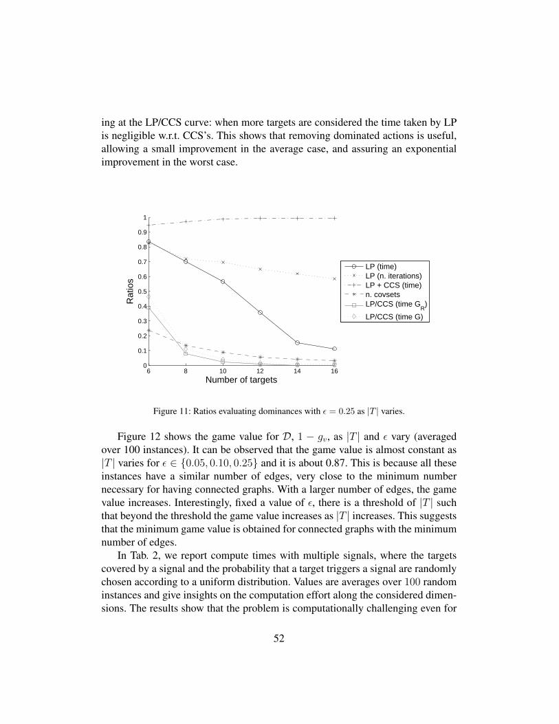
ing at the LP/CCS curve: when more targets are considered the time taken by LPis negligible w.r.t. CCS’s. This shows that removing dominated actions is useful,allowing a small improvement in the average case, and assuring an exponentialimprovement in the worst case.
6 8 10 12 14 160
0.1
0.2
0.3
0.4
0.5
0.6
0.7
0.8
0.9
1
Number of targets
Rat
ios
LP (time)LP (n. iterations)LP + CCS (time)n. covsetsLP/CCS (time G
R)
LP/CCS (time G)
Figure 11: Ratios evaluating dominances with ε = 0.25 as |T | varies.
Figure 12 shows the game value for D, 1 − gv, as |T | and ε vary (averagedover 100 instances). It can be observed that the game value is almost constant as|T | varies for ε ∈ 0.05, 0.10, 0.25 and it is about 0.87. This is because all theseinstances have a similar number of edges, very close to the minimum numbernecessary for having connected graphs. With a larger number of edges, the gamevalue increases. Interestingly, fixed a value of ε, there is a threshold of |T | suchthat beyond the threshold the game value increases as |T | increases. This suggeststhat the minimum game value is obtained for connected graphs with the minimumnumber of edges.
In Tab. 2, we report compute times with multiple signals, where the targetscovered by a signal and the probability that a target triggers a signal are randomlychosen according to a uniform distribution. Values are averages over 100 randominstances and give insights on the computation effort along the considered dimen-sions. The results show that the problem is computationally challenging even for
52

6 8 10 12 14 160.8
0.85
0.9
0.95
1
Number of targets
Val
ues
ε = 0.05ε = 0.10ε = 0.25ε = 0.50ε = 0.75ε = 1.00
Figure 12: Optimal game values as |T | and ε vary.
a small number of targets and signals.
PPPPPPPPPm|T (s)|
5 10 15
2 - 17.83 510.613 - 33.00 769.304 0.55 35.35 1066.765 0.72 52.43 1373.32
Table 2: Compute times (in seconds) for multi–signal instances.
6.1.3. Approximation algorithmsWe evaluate the actual approximation ratios obtained with our approximation
algorithms as (1− gv)/(1− gv), where gv is the expected utility of A at the equi-librium considering all the covering sets and gv is the expected utility of A at theequilibrium when covering sets are generated by our heuristic algorithm. We exe-cute our approximation dynamic programming algorithm with a different number,say RandRes, of randomly generated orders from 10, 20, 30, 40, 50, in addi-tion to the 3 heuristics discussed in Section 3.2.2. We executed our approximationbranch and bound algorithm with constant values of ρ from 0.25, 0.50, 0.75, 1.00(we recall that with ρ = 1.00 backtracking is completely disabled).
53

Figure 13 and Figure 14 report the actual approximation ratios (averaged over100 instances) obtained with our approximation algorithms for different valuesof |T | ∈ 6, 8, 10, 12, 14, 16, i.e., the instances for which we know the optimalgame value, and ε ∈ 0.05, 0.10, 0.25, 0.50, 0.75, 1.00. We remark that the ra-tios obtained with the approximation branch–and–bound algorithm for some val-ues of ρ are omitted. This is because the compute time needed by the algorithmis over 104 seconds. The algorithm always terminates by the deadline for onlyρ ∈ 0.75, 1.00. We focus on the ratios obtained with the dynamic programmingalgorithm. Given a value of ε, as |T | increases, the ratio decreases up to a giventhreshold of |T | and then it is a constant. The threshold increases as ε decreases,while the constant decreases as ε decreases. The value of the constant is high forevery ε, being larger than 0.8. Although the ratios increase as RandRes increases,it is worth noting that the increase is not very significant, being of the order of0.05 between 10 RandRes and 50 RandRes. We focus on the ratios obtained withthe branch–and–bound algorithm. Given a value of ε, as |T | increases, the ratiodecreases up to a given threshold of |T | and then it increases approaching a ratioof 1. The threshold increases as ε decreases, while the minimum ratio decreasesas ε decreases. Interestingly, ratios with ρ = 1.00 are very close to ratios withρ ∈ 0.75, showing that performing even significant backtracking around the so-lution found with ρ = 1.00 does not lead to a significant improvement of thesolution. The solution can be effectively improved only with ρ = 0.25, but it isnot affordable due to the excessive required compute time. This shows that theheuristic performs very well. Comparing the ratios of the two algorithms, it canbe observed that the approximation dynamic programming algorithm performsbetter than the approximation branch–and–bound algorithm. While the dynamicprogramming one always provides a ratio larger than 0.8, the branch–and–boundone provides for combinations of |T | and ε ratios lower than 0.4.
Figure 15 reports the game values obtained with the approximation dynamicprogramming algorithm for every value of RandRes and with the approximationbranch–and–bound algorithm when |T | ∈ 20, 25, 30, 35, 40, 45, 50 only for ρ =1.00. Indeed, with ρ = 0.75 the compute time is excessive and, as shown above,the purely heuristic solution cannot be significantly improved for ε ≥ 0.75. Wereport experimental results only for ε ∈ 0.05, 0.25. We notice that for theseinstances we do not have the optimal game value. However, since the optimalgame value cannot be larger than 1 by construction of the instances, the gamevalue obtained with our approximation algorithms represents a lower bound to theactual approximation ratio. It can be observed that, given a value of ε, the ratiosobtained with the dynamic programming algorithm are essentially constant as |T |
54

ε=
0.05
6 8 10 12 14 160.4
0.5
0.6
0.7
0.8
0.9
1
Number of targets
Rat
ios
(val
ues)
10 RandRes20 RandRes30 RandRes40 RandRes50 RandRes
6 8 10 12 14 160.4
0.5
0.6
0.7
0.8
0.9
1
Number of targets
Rat
ios
(val
ues)
ρ=0.25ρ=0.5ρ=0.75ρ=1
ε=
0.10
6 8 10 12 14 160.4
0.5
0.6
0.7
0.8
0.9
1
Number of targets
Rat
ios
(val
ues)
10 RandRes20 RandRes30 RandRes40 RandRes50 RandRes
6 8 10 12 14 160.4
0.5
0.6
0.7
0.8
0.9
1
Number of targets
Rat
ios
(val
ues)
ρ=0.25ρ=0.5ρ=0.75ρ=1
ε=
0.25
6 8 10 12 14 160.4
0.5
0.6
0.7
0.8
0.9
1
Number of targets
Rat
ios
(val
ues)
10 RandRes20 RandRes30 RandRes40 RandRes50 RandRes
6 8 10 12 14 160.4
0.5
0.6
0.7
0.8
0.9
1
Number of targets
Rat
ios
(val
ues)
ρ=0.25ρ=0.5ρ=0.75ρ=1
Dynamic programming based approximation Branch and bound based approximation
Figure 13: Approximation ratios as |T | varies.
55

ε=
0.50
6 8 10 12 14 160.4
0.5
0.6
0.7
0.8
0.9
1
Number of targets
Rat
ios
(val
ues)
10 RandRes20 RandRes30 RandRes40 RandRes50 RandRes
6 8 10 12 14 160.4
0.5
0.6
0.7
0.8
0.9
1
Number of targets
Rat
ios
(val
ues)
ρ=0.25ρ=0.5ρ=0.75ρ=1
ε=
0.75
6 8 10 12 14 160.4
0.5
0.6
0.7
0.8
0.9
1
Number of targets
Rat
ios
(val
ues)
10 RandRes20 RandRes30 RandRes40 RandRes50 RandRes
6 8 10 12 14 160.4
0.5
0.6
0.7
0.8
0.9
1
Number of targets
Rat
ios
(val
ues)
ρ=0.25ρ=0.5ρ=0.75ρ=1
ε=
1.00
6 8 10 12 14 160.4
0.5
0.6
0.7
0.8
0.9
1
Number of targets
Rat
ios
(val
ues)
10 RandRes20 RandRes30 RandRes40 RandRes50 RandRes
6 8 10 12 14 160.4
0.5
0.6
0.7
0.8
0.9
1
Number of targets
Rat
ios
(val
ues)
ρ=0.25ρ=0.5ρ=0.75ρ=1
Dynamic programming based approximation Branch and bound based approximation
Figure 14: Approximation ratios as |T | varies.
56

ε = 0.05 ε = 0.25
20 25 30 35 40 45 500
0.5
1
1.5
Number of targets
Val
ues
10 RandRes20 RandRes30 RandRes40 RandRes50 RandResρ = 1
20 25 30 35 40 45 500
0.5
1
1.5
Number of targets
Val
ues
10 RandRes20 RandRes30 RandRes40 RandRes50 RandResρ = 1
Figure 15: Game values as |T | varies.
increases and this constant reduced as ε reduces. Surprisingly, after a certain valueof |T |, the game values obtained with the branch and bound algorithm are higherthan those obtained with the dynamic programming algorithm. This is because,fixed a value of ε, as |T | increases, the problem becomes easier and the heuristicused by the branch and bound algorithm performs well finding the best coveringroutes. This shows that there is not an algorithm outperforming the other for everycombination of parameters |T | and ε. Furthermore, the above result shows thatthe worst cases for the approximation algorithms are those in which ε = O( 1
|T |),corresponding to instances in which the number of edges per vertex is a constantin |T |. It is not clear from our experimental analysis whether increasing |T | withε = ν
|T | for some ν > 1 the game value approaches to 0 or to a strictly positivevalue. However, our approximation algorithms provide a very good approximationeven with a large number of targets and a small value of ε.
Figure 16 reports the compute times required by the approximation dynamicprogramming algorithms. As it can be seen, the required time slightly increaseswhen adopting a larger number of randomly generated orders with respect to thebaseline with ρ = 1.00.
6.2. Real case studyIn this section we present the results obtained by applying our approach to a
real case study, in order to show an example of real application of our model. Weimagine to face the task of protecting a fair site as we already discussed in Sec-tion 1.1.2 and we focus on the particular setting of Expo 2015. Figure 17 showsthe map of the Expo 2015 site together with its graph representation. We manually
57

ε = 0.05 ε = 0.25
20 25 30 35 40 45 5010
0
101
102
103
104
Number of targets
Tim
es (
s)
10 RandRes20 RandRes30 RandRes40 RandRes50 RandResρ = 1.00
20 25 30 35 40 45 5010
0
101
102
103
104
Number of targets
Tim
es (
s)
10 RandRes20 RandRes30 RandRes40 RandRes50 RandResρ = 1.00
Figure 16: Time ratios as |T | varies.
build a discretized version of the site map by exploiting publicly available knowl-edge of the event8. We identify ≈ 170 sensible locations which correspond to anequal number of targets in our graph. More specifically, we identify ≈ 130 targetslocated at the entrances of each pavilion and in the surroundings of those areaswhich could be of interest for a high number of visitors. Some targets (≈ 35) arelocated over the main roads, being these critical mainly due to their high crowd.Such roads also define our set of edges which resulted in a density of ≈ 0.02.Figure 17 reports a graphical representation of chosen deadlines d(·) and valuesπ(·), respectively. To determine such values in a reasonable way we apply a num-ber of simple rules of thumb. First, to ease our task, we discretize the spaces ofpossible deadlines and values in four different levels. To assign a value to a target,we estimate the interest (in terms of popularity and expected crowd) of the corre-sponding area in the fair site. The higher the interest, the higher the value (actualvalues are reported in the figure). To assign deadlines we estimate the time anattacker should spend to escape from the attacked target after some malicious ac-tivity is started (for example, blending into the crowd without leaving any trace).In particular, we estimate a smaller escape time for those locations lying near theexternal border of the fair site while for locations that are more central we esti-mated a larger time. The smaller the escape time, the tighter the deadline for thattarget. Actual values are extracted from a normal distribution where σ2 = 1 andµ is set according to the chosen level. The maximum distance between any twotarget locations is about 1.5Km which we assume can be be covered in about 7.5
8Detailed information can be found at http://www.expo2015.org/.
58

Rea
lmap
Gra
phon
real
map
Val
ues
Dea
dlin
es
Figure 17: Expo 2015 instance.
59

minutes (we imagined a crowded scenario). Given such reference scenario, ourmeans span from 5 minutes (very tight) to 7.5 minutes (very large). To derive ouralarm system model we assume to have a number of panoramic cameras deployedin the environment at locations we manually choose in order to cover the wholeenvironment and to guarantee a wide area of view for each camera (i.e., trying tokeep, in general, more than one target under each camera’s view). To map our setof cameras over the alarm system model, we adopt this convention: each group ofcameras sharing an independent partial view of a target t is associated to a signals ∈ S(t); if target t is covered by k signals then each signal is generated withprobability 1/k once t is attacked. Obviously, a deeper knowledge of the securitysystems deployed on the site can enable specific methods to set the parametersof our model. This is why we encourage involving agencies in charge of securitywhen dealing with such task.
Figure 18: Best placement and attack locations.
We first show a qualitative evaluation of our method. Figure 18 depicts thebest placement for the Defender (the circle in the figure) and the attacked tar-gets (the squares in the figure, these are the actions played by the Attacker withnon–null probability at the equilibrium). As intuition would suggest, the best lo-cation from where any signal response should start is a central one w.r.t. the wholefair site. Our simulations show that the optimal patrolling strategy coincides withsuch fixed placement even under false negatives rates of at least ≈ 0.3. Noticethat such false negatives value can be considered unrealistically pessimistic foralarm systems deployed in structured environment like the one we are dealing
60

Covering set Probability19, 20, 23, 25, 125, 126, 127, 128 0.019410, 12, 23, 24, 25, 126, 127, 128 0.023110, 12, 24, 25, 126, 127, 128, 129 0.033312, 23, 24, 25, 126, 127, 128, 129 0.049410, 12, 23, 24, 25, 125, 126, 128 0.034410, 12, 24, 25, 125, 126, 128, 129 0.048810, 12, 25, 125, 126, 127, 128, 129 0.049312, 23, 24, 25, 125, 126, 127, 128 0.050212, 24, 25, 125, 126, 127, 128, 129 0.069219, 20, 23, 25, 125, 126, 129 0.049219, 20, 23, 125, 126, 128, 129 0.049220, 23, 25, 126, 127, 128, 129 0.065710, 23, 25, 125, 126, 127, 128 0.066219, 20, 23, 25, 125, 128, 129 0.041223, 25, 125, 126, 127, 128, 129 0.114620, 23, 24, 25, 127, 128 0.064510, 12, 24, 125, 126, 127 0.087720, 23, 24, 25, 128, 129 0.0846
Figure 19: Example of response strategies to signal.
61
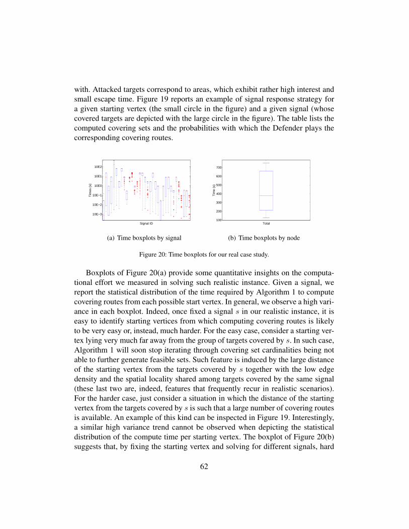
with. Attacked targets correspond to areas, which exhibit rather high interest andsmall escape time. Figure 19 reports an example of signal response strategy fora given starting vertex (the small circle in the figure) and a given signal (whosecovered targets are depicted with the large circle in the figure). The table lists thecomputed covering sets and the probabilities with which the Defender plays thecorresponding covering routes.
10E−3
10E−2
10E−1
10E0
10E1
10E2
Signal ID
Tim
es (
s)
(a) Time boxplots by signal
100
200
300
400
500
600
700
Total
Tim
e (s
)
(b) Time boxplots by node
Figure 20: Time boxplots for our real case study.
Boxplots of Figure 20(a) provide some quantitative insights on the computa-tional effort we measured in solving such realistic instance. Given a signal, wereport the statistical distribution of the time required by Algorithm 1 to computecovering routes from each possible start vertex. In general, we observe a high vari-ance in each boxplot. Indeed, once fixed a signal s in our realistic instance, it iseasy to identify starting vertices from which computing covering routes is likelyto be very easy or, instead, much harder. For the easy case, consider a starting ver-tex lying very much far away from the group of targets covered by s. In such case,Algorithm 1 will soon stop iterating through covering set cardinalities being notable to further generate feasible sets. Such feature is induced by the large distanceof the starting vertex from the targets covered by s together with the low edgedensity and the spatial locality shared among targets covered by the same signal(these last two are, indeed, features that frequently recur in realistic scenarios).For the harder case, just consider a situation in which the distance of the startingvertex from the targets covered by s is such that a large number of covering routesis available. An example of this kind can be inspected in Figure 19. Interestingly,a similar high variance trend cannot be observed when depicting the statisticaldistribution of the compute time per starting vertex. The boxplot of Figure 20(b)suggests that, by fixing the starting vertex and solving for different signals, hard
62

instances counterbalance, on average, the easy ones.
7. Related works
In the last few years, Security Games received an increasing interest from theArtificial Intelligence scientific community, leading to the exploration of a largenumber of research directions around this topic. In this section, we briefly discusswhat we deem to be the most significant ones, starting from the game theoreticalfoundations on which these models are built.
Computing solution concepts is the central problem upon which the real appli-cability of these game theoretical models is based. A lot of works concentrated onalgorithmic studies of this topic, analysing the relationships holding among dif-ferent kinds of solution concepts and their computational complexity. In [40] therelationship between Stackelberg, Nash and min–max equilibria is studied, whilein [41] some refinements of the Stackelberg equilibrium are proposed. Many ef-forts have been made to develop tractable algorithms for finding Stackelberg equi-libria in Bayesian games [42]. Furthermore, in [43] the authors analysed scenariosin which the Defender has multiple objectives, searching for the Pareto curve ofthe Stackelberg equilibria.
Besides fundamental works like the ones cited above, a more recent researchline devoted efforts towards the definition of game model refinements in the at-tempt to overcome some of their ideal assumptions. One remarkable issue belong-ing to this scope is how to model the behaviour of the Attacker. In the attempt tohave a more realistic behaviour, some works considered bounded rationality anddefined algorithms to deal with it. In [44] different models of the Attacker are anal-ysed while in [45, 46] the Attacker is allowed to have different observation andplanning capabilities. Moreover, in [47] Quantal–Best Response is used to modelthe behaviour of the Attacker and in [48] algorithms that scale up with boundedrational adversaries are proposed. In our paper, we assume that the attacker isrational.
Other model refinements focused on those cases in which games exhibit spe-cific structures that can be leveraged in the design of algorithms to compute theStackelberg equilibrium. For instance, the study of the spread of contagion overa network is investigated in [49]. When no scheduling constraints are present andpayoffs exhibit a special form, the computation of a Stackelberg equilibrium canbe done very efficiently enabling the resolution of remarkably big scenarios [50].In [51] realistic aspects of infrastructures to be protected are taken into account.
63

8. Conclusions and future research
In this paper we provide the first Security Game for large environments surveil-lance, e.g. for fair sites protection, that can exploit an alarm system with spatiallyuncertain signals. To monitor and protect large infrastructure such as stations, air-ports, and cities, a two–level paradigm is commonly adopted: a broad area surveil-lance phase, where an attack is detected but only approximately localized due tothe spatially uncertainty of the alarm system, triggers a local investigation phase,where guards have to find and clear the attack. Abstracting away from techno-logical details, we propose a simple model of alarm systems that can be widelyadopted with every specific technology and we include it in the state–of–art pa-trolling models, obtaining a new security game model. We show that the problemof finding the best patrolling strategy to respond to a given alarm signal isAPX–hard with arbitrary graphs even when the game is zero–sum. Then, we provide twoexponential–time exact algorithms to find the best patrolling strategy to respondto a given alarm signal. The first algorithm performs a breath–first search by ex-ploiting a dynamic programming approach, while the second algorithm performsa depth–first approach by exploiting a branch–and–bound approach. We providealso a variation of these two algorithms to find an approximate solution. We ex-perimentally evaluate our exact and approximation algorithms both in worst–caseinstances, to evaluate empirically the gap between our hardness results and the the-oretical guarantees of our approximation algorithms, and in one realistic instance,Expo 2015. The limit of our exact algorithms is about 16 targets with worst–case instances while we were able to compute an optimal solution for a realisticinstance with≈ 170 targets. On the other side, our approximation algorithms pro-vide a very effective approximation even with worst–case instances. We providealso results for special topologies, showing that our dynamic programming algo-rithm requires polynomial time with linear and cycle graphs, while the problemis NP–hard with tree graphs. Finally, we focus on the problem of patrolling theenvironment, showing that if every target is alarmed and no false positives andmissed detections are present, then the best patrolling strategy prescribes that thepatroller stays in a given place waiting for an alarm signal. Furthermore, we showthat such a strategy may be optimal even for missed detection rates up to 50%.
Of course, our research does not end here since some problems related to ourmodel remain open. The main theoretical issue is the closure of the approximationgap of SRG–v. We believe that investigating the relationship between our modeland the DEADLINE–TSP could help in closing the gap. Another interesting prob-lem is the study of approximation algorithms for tree graphs. Our NP–hardness
64

result does not exclude the existence of a PTAS (i.e., polynomial time approxi-mation scheme), even if we conjecture that the existence is unlikely. In addition,a number of extensions of our model are worth being explored. The most im-portant extension is to include false positives and missed detections, allowing thepatroller to patrol even in absence of alarm signals. Other interesting extensionsregard cases in which the number of patrollers is larger than one or there aremultiple attackers, which coordinate to perform their malicious attack. Finally, adifferent research direction stemming from the problem concerns the alarm sys-tem dimension. Indeed, trying to deploy sensors and devices in the environmentin such a way to maximize the utility in responding to alarms is a non–trivial andinteresting problem, mainly due to the inherent budget constraint and trade–offsthat would exhibit.
References
[1] M. Jain, B. An, M. Tambe, An overview of recent application trends at theAAMAS conference: Security, sustainability, and safety, AI Magazine 33 (3)(2012) 14–28.
[2] B. Von Stengel, S. Zamir, Leadership with commitment to mixed strategies,Tech. rep. (2004).
[3] V. Conitzer, T. Sandholm, Computing the optimal strategy to commit to, in:Proceedings of the 7th ACM Conference on Electronic Commerce, 2006,pp. 82–90.
[4] J. Pita, M. Jain, C. Western, C. Portway, M. Tambe, F. Ordonez, S. Kraus,P. Paruchuri, Deployed armor protection: The application of a game-theoretic model for security at the los angeles international airport, in: Pro-ceedings of the International Joint Conference on Autonomous Agents andMulti–Agent Systems (AAMAS), 2008, pp. 125–132.
[5] J. Tsai, S. Rathi, C. Kiekintveld, F. Ordonez, M. Tambe, Iris – a tool forstrategic security allocation in transportation networks, in: Proceedings ofthe International Joint Conference on Autonomous Agents and Multi–AgentSystems (AAMAS), 2009, pp. 1327–1334.
[6] B. An, E. Shieh, R. Yang, M. Tambe, C. Baldwin, J. DiRenzo, B. Maule,G. Meyer, Protect – a deployed game theoretic system for strategic security
65

allocation for the united states coast guard, AI Magazine 33 (4) (2014) 96–110.
[7] F. M. Delle Fave, A. X. Jiang, Z. Yin, C. Zhang, M. Tambe, S. Kraus, J. Sulli-van, Game–theoretic security patrolling with dynamic execution uncertaintyand a case study on a real transit system, Journal of Artificial IntelligenceResearch 50 (2014) 321–367.
[8] B. Ford, D. Kar, F. M. Delle Fave, R. Yang, M. Tambe, Paws: Adaptivegame-theoretic patrolling for wildlife protection, in: International Confer-ence on Autonomous Agents and Multi–Agent Systems (AAMAS), 2014,pp. 1641–1642.
[9] N. Basilico, N. Gatti, F. Amigoni, Patrolling security games: Definition andalgorithms for solving large instances with single patroller and single in-truder, ARTIF INTELL 184–185 (2012) 78–123.
[10] N. Basilico, N. Gatti, F. Villa, Asynchronous multi-robot patrolling againstintrusion in arbitrary topologies, in: Proceedings of the Twenty-Fourth Con-ference on Artificial Intelligence (AAAI), 2010, pp. 1224–1229.
[11] N. Agmon, G. A. Kaminka, S. Kraus, Multi–robot adversarial patrolling:Facing a full–knowledge opponent, Journal of Artificial Intelligence Re-search (JAIR) 42 (2011) 887–916.
[12] E. Sless, N. Agmon, S. Kraus, Multi–robot adversarial patrolling: facing co-ordinated attacks, in: International conference on Autonomous Agents andMulti-Agent Systems (AAMAS), 2014, pp. 1093–1100.
[13] N. Agmon, C. Fok, Y. Emaliah, P. Stone, C. Julien, S. Vishwanath, On co-ordination in practical multi-robot patrol, in: IEEE International Conferenceon Robotics and Automation (ICRA), 2012, pp. 650–656.
[14] Y. Vorobeychik, B. An, M. Tambe, S. P. Singh, Computing solutions ininfinite–horizon discounted adversarial patrolling games, in: Proceedingsof the Twenty-Fourth International Conference on Automated Planning andScheduling (ICAPS), 2014, pp. 314–322.
[15] E. A. Shieh, M. Jain, A. X. Jiang, M. Tambe, Efficiently solving joint ac-tivity based security games, in: Proceedings of the 23rd International JointConference on Artificial Intelligence (IJCAI), 2013, pp. 346–352.
66

[16] J. Gan, B. An, Y. Vorobeychik, Security games with protection externalities,in: Proceedings of the Twenty-Ninth Conference on Artificial Intelligence(AAAI), 2015, pp. 914–920.
[17] N. Agmon, On events in multi-robot patrol in adversarial environments, in:International conference on Autonomous Agents and Multi–Agent Systems(AAMAS), 2010, pp. 591–598.
[18] S. Alpern, A. Morton, K. Papadaki, Patrolling games, Operations Research59 (5) (2011) 1246–1257.
[19] N. Basilico, S. Carpin, T. Chung, Distributed online patrolling with multi-agent teams of sentinels and searchers, in: DARS, 2014.
[20] B. C. Ko, J. O. Park, J.-Y. Nam, Spatiotemporal bag-of-features for earlywildfire smoke detection, Image and Vision Computing 31 (10) (2013) 786– 795.
[21] A.-J. Garcia-Sanchez, F. Garcia-Sanchez, J. Garcia-Haro, Wireless sensornetwork deployment for integrating video-surveillance and data-monitoringin precision agriculture over distributed crops, Computers and Electronics inAgriculture 75 (2) (2011) 288 – 303.
[22] J. Yick, B. Mukherjee, D. Ghosal, Wireless sensor network survey, Comput.Netw. 52 (12) (2008) 2292–2330.
[23] Z. Sun, P. Wang, M. C. Vuran, M. A. Al-rodhaan, A. M. Al-dhelaan, I. F.Akyildiz, Bordersense: Border patrol through advanced wireless sensor net-works, Ad Hoc Networks 9 (3) (2011) 468 – 477.
[24] A. Krause, A. Roper, D. Golovin, Randomized sensing in adversarial envi-ronments, in: Proceedings of the International Joint Conference on ArtificialIntelligence, Barcelona, 2011, pp. 2133–2139.
[25] E. Munoz de Cote, R. Stranders, N. Basilico, N. Gatti, N. Jennings, Introduc-ing alarms in adversarial patrolling games, in: International conference onAutonomous Agents and Multi–Agent Systems (AAMAS), 2013, pp. 1275–1276.
[26] N. Basilico, N. Gatti, Strategic guard placement for optimal response toalarms in security games, in: International conference on AutonomousAgents and Multi–Agent Systems (AAMAS), 2014, pp. 1481–1482.
67
[27] N. Basilico, N. Gatti, T. Rossi, S. Ceppi, F. Amigoni, Extending algorithmsfor mobile robot patrolling in the presence of adversaries to more realisticsettings, in: Proceedings of the 2009 IEEE/WIC/ACM International Confer-ence on Intelligent Agent Technology (IAT), 2009, pp. 557–564.
[28] N. Basilico, N. Gatti, T. Rossi, Capturing augmented sensing capabilitiesand intrusion delay in patrolling-intrusion games, in: IEEE Symposium onComputational Intelligence and Games (CIG), 2009, pp. 186–193.
[29] Y. Shoham, K. Leyton-Brown, Multiagent Systems: Algorithmic, Game-Theoretic, and Logical Foundations, Cambridge University Press, New York,NY, USA, 2008.
[30] M. Maschler, S. Zamir, E. Solan, Game Theory, Cambridge University Press,2013.
[31] M. R. Garey, D. S. Johnson, Computers and Intractability; A Guide to theTheory of NP-Completeness, W. H. Freeman & Co., New York, NY, USA,1990.
[32] M. J. Osborne, An introduction to game theory, Vol. 3, Oxford UniversityPress New York, 2004.
[33] C. H. Papadimitriou, M. Yannakakis, The traveling salesman problem withdistances one and two, Mathematics of Operations Research 18 (1) (1993)1–11.
[34] H.-J. Bckenhauer, J. Hromkovic, J. Kneis, J. Kupke, The parameterizedapproximability of tsp with deadlines, Theory Computing Systems 41 (3)(2007) 431–444.
[35] N. Bansal, A. Blum, S. Chawla, A. Meyerson, Approximation algorithms fordeadline-tsp and vehicle routing with time-windows, in: Proceedings of theThirty-sixth Annual ACM Symposium on Theory of Computing (STOC),2004, pp. 166–174.
[36] E. Lawler, Combinatorial Optimization: Networks and Matroids, DoverBooks on Mathematics, 2011.
[37] M. W. Savelsbergh, Local search in routing problems with time windows,ANN OPER RES 4 (1) (1985) 285–305.
68

[38] R. W. Conway, W. L. Maxwell, L. W. Millerr, Theory of scheduling, DoverBooks on Mathematics, 2003.
[39] H.-J. Bockenhauer, L. Forlizzi, J. Hromkovic, J. Kneis, J. Kupke, G. Proi-etti, P. Widmayer, Reusing optimal tsp solutions for locally modified inputinstances, in: IFIP TCS, 2006, pp. 251–270.
[40] D. Korzhyk, Z. Yin, C. Kiekintveld, V. Conitzer, M. Tambe, Stackelbergvs. nash in security games: An extended investigation of interchangeabil-ity, equivalence, and uniqueness, Juornal of Artificial Intelligence Research(JAIR) 41 (2011) 297–327.
[41] B. An, M. Tambe, F. Ordonez, E. A. Shieh, C. Kiekintveld, Refinementof strong stackelberg equilibria in security games, in: Proceedings of theTwenty-Fifth Conference on Artificial Intelligence (AAAI), 2011, pp. 587–593.
[42] M. Jain, C. Kiekintveld, M. Tambe, Quality–bounded solutions for finitebayesian stackelberg games: scaling up, in: International Conference onAutonomous Agents and Multi–Agent Systems (AAMAS), 2011, pp. 997–1004.
[43] M. Brown, B. An, C. Kiekintveld, F. Ordonez, M. Tambe, An extended studyon multi–objective security games, Autonomous Agents and Multi–AgentSystems (AAMAS) 28 (1) (2014) 31–71.
[44] T. H. Nguyen, R. Yang, A. Azaria, S. Kraus, M. Tambe, Analyzing theeffectiveness of adversary modeling in security games, in: Proceedings ofthe Twenty-Seventh Conference on Artificial Intelligence (AAAI), 2013, pp.718–724.
[45] B. An, M. Brown, Y. Vorobeychik, M. Tambe, Security games with surveil-lance cost and optimal timing of attack execution, in: International confer-ence on Autonomous Agents and Multi–Agent Systems (AAMAS), 2013,pp. 223–230.
[46] R. Yang, B. Ford, M. Tambe, A. Lemieux, Adaptive resource allocation forwildlife protection against illegal poachers, in: International Conference onAutonomous Agents and Multiagent Systems (AAMAS), 2014, pp. 453–460.
69

[47] B. An, F. Ordonez, M. Tambe, E. Shieh, R. Yang, C. Baldwin, J. DiRenzo,K. Moretti, B. Maule, G. Meyer, A deployed quantal response–based patrolplanning system for the U.S. coast guard, Interfaces 43 (5) (2013) 400–420.
[48] R. Yang, A. X. Jiang, M. Tambe, F. Ordonez, Scaling–up security gameswith boundedly rational adversaries: A cutting–plane approach, in: Proceed-ings of the International Joint Conference on Artificial Intelligence (IJCAI),2013, pp. 404–410.
[49] J. Tsai, T. H. Nguyen, N. Weller, M. Tambe, Game–theoretic target selectionin contagion–based domains, The Computer Journal 57 (6) (2014) 893–905.
[50] C. Kiekintveld, M. Jain, J. Tsai, J. Pita, F. Ordonez, M. Tambe, Computingoptimal randomized resource allocations for massive security games, in: In-ternational Joint Conference on Autonomous Agents and Multi–Agent Sys-tems (AAMAS), 2009, pp. 689–696.
[51] A. Blum, N. Haghtalab, A. D. Procaccia, Lazy defenders are almost optimalagainst diligent attackers, in: Proceedings of the Twenty-Eighth Conferenceon Artificial Intelligence (AAAI), 2014, pp. 573–579.
Appendix A. Notation
We report in Tab. A.3 the symbols used along the paper.
Appendix B. Additional experimental results
We report in Fig. B.21 the boxplots of the results depicted in Fig. 10. Theyshow that the variance of the compute times drastically reduces as ε increases.This is because the number of edges increases as ε increases and so the numberof proper covering sets increases approaching 2|T |. On the other hand, with smallvalues of ε, the number of proper covering sets of different instances can be ex-tremely different.
70
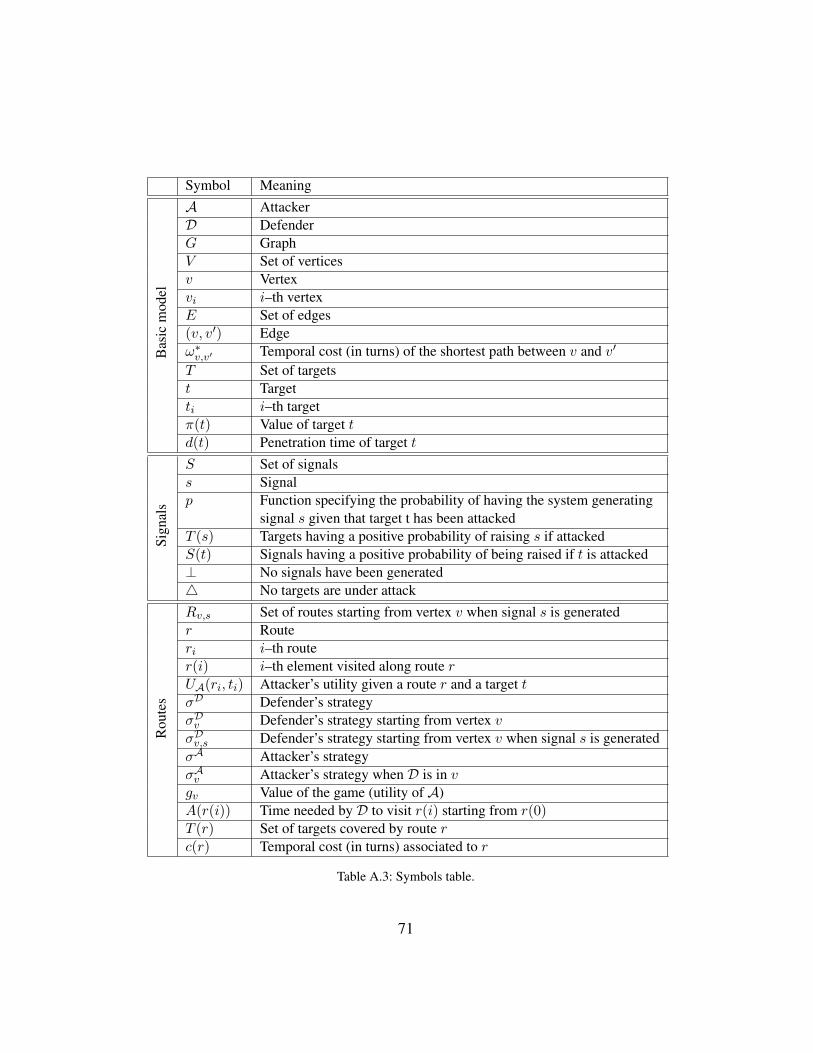
Symbol Meaning
Bas
icm
odel
A AttackerD DefenderG GraphV Set of verticesv Vertexvi i–th vertexE Set of edges(v, v′) Edgeω∗v,v′ Temporal cost (in turns) of the shortest path between v and v′
T Set of targetst Targetti i–th targetπ(t) Value of target td(t) Penetration time of target t
Sign
als
S Set of signalss Signalp Function specifying the probability of having the system generating
signal s given that target t has been attackedT (s) Targets having a positive probability of raising s if attackedS(t) Signals having a positive probability of being raised if t is attacked⊥ No signals have been generated4 No targets are under attack
Rou
tes
Rv,s Set of routes starting from vertex v when signal s is generatedr Routeri i–th router(i) i–th element visited along route rUA(ri, ti) Attacker’s utility given a route r and a target tσD Defender’s strategyσDv Defender’s strategy starting from vertex vσDv,s Defender’s strategy starting from vertex v when signal s is generatedσA Attacker’s strategyσAv Attacker’s strategy when D is in vgv Value of the game (utility of A)A(r(i)) Time needed by D to visit r(i) starting from r(0)T (r) Set of targets covered by route rc(r) Temporal cost (in turns) associated to r
Table A.3: Symbols table.
71

ε=
0.05
10−1
100
101
102
103
104
6 8 10Number of targets
Tim
es (
s)
ε=
0.10
10−1
100
101
102
103
104
6 8 10Number of targets
Tim
es (
s)
ε=
0.25
10−1
100
101
102
103
104
6 8 10 12 14 16Number of targets
Tim
es (
s)
ε=
0.50
10−1
100
101
102
103
104
6 8 10 12 14 16Number of targets
Tim
es (
s)
ε=
0.75
10−1
100
101
102
103
104
6 8 10 12 14 16Number of targets
Tim
es (
s)
ε=
1.00
10−1
100
101
102
103
104
6 8 10 12 14 16Number of targets
Tim
es (
s)
Figure B.21: Boxplots of compute times required by our exact dynamic programming algorithm.
72