advances in surface penetrating technologies for …web.eecs.umich.edu/~aey/phd/marbles.pdf ·...

Advances in Surface PenetratingTechnologies for Imaging, Detection,

and Classification

FinalDefense

Jay A. Marble

Committee: Alfred Hero (co-chair)Andrew Yagle (co-chair)Eric MichielssenMahta Moghaddam

Surface Penetrating TechnologiesProblem Statement

l General Problem – Objects of interest in an unknown, inhomogeneous media.

l The ultimate goal is to detect and identify the objects of interest while ignoring the clutter.

l The scope of the problem rangesfrom initial object imaging,to detection, to final classification.

l Classification also includes thescheduling of confirmation sensors.

Free Space

Inner Region 1Inner Region 2

OuterSurface

InnerSurface

Objectof Interest

Objectof

InterestClutter

Clutter

Clutter

Clutter

Clutter

Free Space

Inner Region 1Inner Region 2

OuterSurface

InnerSurface

Objectof Interest

Objectof

InterestClutter

Clutter

Clutter

Clutter

Clutter

SpecializedConfirmation Sensor

LargeAreaScanner

TransmitReceivePair

l Landmine/UXO Detectionl Ground Penetrating Radar imaging.l Detect and discriminate between landmines and

various clutter objects.l Sensor scheduling of confirmation sensors.

l See-Through-Wall Radar Imagingl Provide authorities with accurate information

concerning building interiors.l This can include: hidden weapons, building layouts,

suspicious person tracking, methamphetamine labs.l Sensor scheduling for adaptive imaging.

Applications

NOT Landmine

Landmine

Discriminate between landmines andother objects using multiple sensors.

ApplicationsLandmine Detection/Classification

ApplicationsSee-Through-Wall Imaging

l Problems of InterestLayout Mapping of Inner WallsCache DetectionSuspicious Person Tracking

l Technical ChallengesInhomogeneous Medium

Causes multipath scattering - ghostsUnknown phase delays through

wall - blurring.Walls may be metal reinforced.

E&M Penetration difficult.Requires higher frequencies,which attenuate faster.

l Non-statistical MethodsSNR EnhancementRadar and Metal Detectors for

Landmine Detection

l Statistical Methods Landmine Scanning Sensors Sensor Scheduling of Landmine

Confirmation Sensors

l Imaging Sensor Scheduling of STW Radar Near Real Time STW and Landmine

Radar Imaging – 2D and 3D

Contribution Areas

Non-statistical Methodsof Signal-to-Noise Ratio Enhancement

l SNR Enhancement of GPR Signalsl Hyperbola Flattening Transforml Makes use of the un-imaged point spread function of

radar echoes from landmines.

l Metal Detector Signal Processingl Electromagnetic Induction (EMI) Sensorsl Utilize a dipole response model to identify basis functions. l Form subspace filters to enhance SNR and identify

object depth and rudimentary shape.

l Vision System Methodsl Generate a focused image of the landmine.l Draw a bounding box around the object to

extract size and depth info.

Non-statistical Methods

Radar SNR Enhancement

Plastic Landmine (VS1.6)SurfaceTop ofMine at 6”SoilStratum

l Deeply buried plastic landmines face a low signal-to-noise ratio (SNR).

l Strata in the ground can create large radar returns that lead to false alarms.

l The Hyperbolic Flattening Transform seeks to exploit all the “energy” of the hyperbolic signature.

The Hyperbola Flattening Transform

Depth into G

round

Vehicle Motion

Simulation Simulation

Original Hyperbola 45° RotationSimulation Simulation

Radar SNR EnhancementHyperbola Flattening Transform

Remapping:1/yy

12

2

2

2

=−ax

dy 1=xy 1=

yx

The Hyperbola Flattening Transform converts a hyperbolicsignature into a straight line at 45°.

Application to Simulated Data

The RADON transform creates “projections” bysumming along lines.

Projections are orientedfor 0° to 180°.

Radon Transform of the “flattened” hyperbola has a

strong maximum at 45°corresponding to the “energy” contained in the hyperbola.

Transform Location ofHyperbolic Signature

Application to Real Data

VS1.6

Along Track

The HFT will now beapplied as a detector.

A small kernel is movedthroughout the scene. Ateach location, the HFT isapplied.,

At each point the HFT is run for several values of the “a” parameter. Themaximum result is placedinto a detection image.

Original Image


VS1.6

The HFT is applied to alllocations in the scene. The detection image shownhere is the result.

Bright pixels correspond to hyperbolas. Hyperbolicsignatures have been contrast enhanced, whilenon-hyperbolas are suppressed.Along Track

Hyperbola Detection Image


VS1.6

Along Track

Pixels that break a certainthreshold are shown.These pixels reveal thelocations of the “most hyperbola-like” signalsin the scene.

The region corresponding to the VS1.6 has been enhanced by the HFTdetector.

Hyperbola-like Regions


l Marble,J., Yagle,A., “The Hyperbola Flattening Transform,” SPIE: Detection and Remediation Technologies for Mines and Minelike Targets IX, April 2004,Orlando, FL.

l Marble,J., Yagle,A., “Measuring Landmine Size and Burial Depth with Ground Penetrating Radar,” SPIE: Detection and Remediation Technologies for Mines and Minelike Targets IX, April 2004, Orlando, FL.

l Marble,J.,Yagle,A., Wakefield,G, “Physics Derived Basis Pursuit in BuriedObject Identification using EMI Sensors,” SPIE: Detection and RemediationTechnologies for Mines and Minelike Targets X, March 2005, Orlando, FL.

Non-statisticalContributions

Statistical Methodsof Landmine Detection

and Classification

l Multimodal Landmine Detectionl Scanning Sensor Algorithml Joint Probability Densities of Two Sensors l Maximum A Posteriori (MAP) Detection/Classification

l Single Confirmation Sensor Schedulingl Information Gain Metric – Rényi Divergencel Deploy Sensor that Provides Greatest Information Gain

l Multiple Confirmation Sensor Schedulingl Collaboration with GATech and Doron Blattl Develop an optimal policy for deploying multiple

sensors. l Reinforcement learning method used for training.

Statistical Methods

Scanning Sensor Observations

GPR Sensor

EMI Sensor

CurrentScanLine

PlatformMotion

Sensor Arrays

GPREMI Platform

Motion

Sensor Arrays

GPREMI

Platform

Location of Objects

100 200 300 400 500 600 700 800 900 1000

10

20

DeepMidShallow

GPR Sensor

100 200 300 400 500 600 700 800 900 1000

10

20

EMI Sensor

100 200 300 400 500 600 700 800 900 1000

10

20

EMI Acquired “Image”

GPR Acquired “Image”

Ground Truth Markings

Metal Landmines OnlySoil Type: Clay

Multimodal Landmine Detection

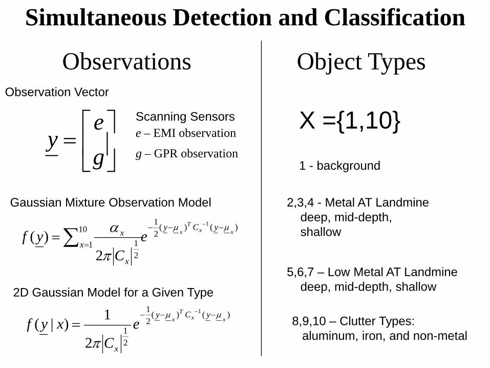
X =1,10

2,3,4 - Metal AT Landminedeep, mid-depth,shallow

5,6,7 – Low Metal AT Landminedeep, mid-depth, shallow

1 - background

8,9,10 – Clutter Types:aluminum, iron, and non-metal

Observations

=

ge

yScanning Sensors

)()(21

10

121

1

2)( xx

Tx yCy

x

x

x eC

yfµµ

π

α −−−

=

−

∑=

Object Types

)()(21

21

1

2

1)|( xxT

x yCy

x

eC

xyfµµ

π

−−− −

=

e – EMI observation

g – GPR observation

Gaussian Mixture Observation Model

Observation Vector

2D Gaussian Model for a Given Type

Simultaneous Detection and Classification

l Supervised Learningl

l From available data the joint PDF of eachobject type is determined.

l Bayes Rule

l

l From the learned distribution we use Bayes rule to translateto the posterior distribution.

l Maximum A Posteriori Detection/Classification

)()(21

21

1

2

1)|( xxT

x yCy

x

eC

xyfµµ

π

−−− −

=

)]|([maxargˆ yxfx x=

)()()|(

)|(yf

xfxyfyxf =

Note: This approach is the same as multiple hypothesis testing on every pixel.

Simultaneous Detection and Classification

• Metal Landmine Composite PDF• The statistics of metal landmines

are favorable for good detectionperformance.

• A similar PDF could be generated for plastic landmines. However,the situation is much less favorable.

• Background pixel PDF showsdecorrelation between EMIand GPR pixel values.

• This decorrelation makes sensor fusion very useful for false-alarmelimination.

EMI Pixel Value

GP

R P

ixel

Val

ue

0 0.5 1 1.5 2 2.5 3 3.5 4 4.5 50

0.05

0.1

0.15

0.2

0.25

0.3

0.35

0.4

0.45

0.5

MetalLandmines

Background“Noise”

Shallow AT

Mid-depth ATDeep AT

Joint Probability Densities

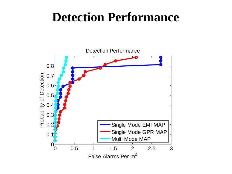
Detection Performance

0 0.5 1 1.5 2 2.5 30

0.1

0.2

0.3

0.4

0.5

0.6

0.7

0.8

False Alarms Per m2

Prob

abilit

y of

Det

ectio

n

Detection Performance

Single Mode EMI MAPSingle Mode GPR MAPMulti Mode MAP

Sensor Scheduling

PlatformMotion

Sensor Arrays

GPREMI Platform

Motion

Sensor Arrays

GPREMI

Platform ScanningSensors

DeployableConfirmationSensor

Other AvailableConfirmation Sensors

Possible Confirmation Sensors:

• E&M: Nuclear Quadrupole Resonance, Magnetometer, Broadband EMI

• Nuclear: X-ray Backscatter, Neutron Excitation

• Other: Chemical “Sniffer”, Acoustic Vibrometer, Mechanical Prodder

l Multiple Landmine Responsesl Four Generic Landmine Classes:

l Environment Impacts Response: Soil Permittivity and Conductivityl Object Depth Impacts Response

l Multiple Landmine Technologiesl Non-exhaustive List: Metal Detectors, RADAR , Magnetometers,

Radiometers, Seismic/Acoustic Vibrometers, Chemical Sensors, Quadrapole Resonance, Touch Probes…

l Each sensor responds differently to landmine types and is impacteddifferently by depth and environment.

l Some sensors are practical in a “scanning” context while other are only practical as “confirmation” sensors.

l Low-metal Anti-Tank l High-metal Anti-Tank

l Low-metal Anti-Personnell High-metal Anti-Personnel

Sensor SchedulingMotivation

Location of Objects 2

200 400 600 800 1000 1200 1400 1600 1800

5

10

15

Location of Objects

200 400 600 800 1000 1200 1400 1600 1800

5

10

15

deep deepmid

shallowmid

shallow

aluminumiron

non-metalmetal mines plastic mines Clutter

Scanning Sensor SimulationsSimulated scanning sensors are used to make the scanning process

realistic. It also gives experimental control over all system parameters and environmental parameters.

Clutter objects (iron, aluminum, and non-metal) have been introduced to study false alarm rejection capabilities of algorithms.

EMI Sensor Simulation

200 400 600 800 1000 1200 1400 1600 1800

5

10

15

GPR Sensor Simulation

200 400 600 800 1000 1200 1400 1600 1800

5

10

15

Sensor N

umber

Sensor N

umber

VehicleMotion

Sample Number

Sample Number

Metal Detector

Ground Penetrating Radar

Scanning Sensor Simulations

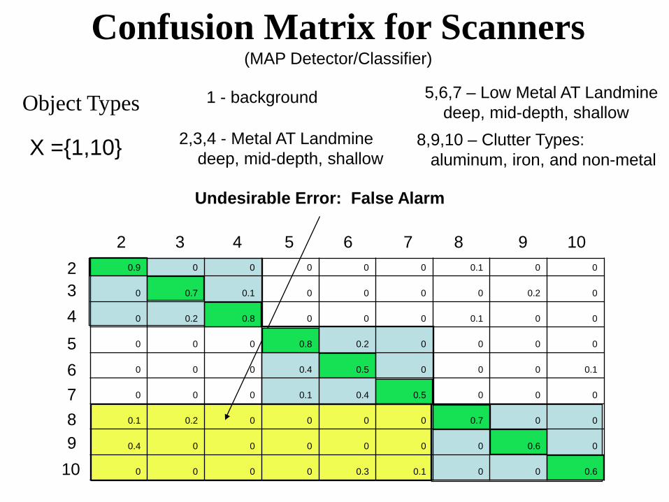
Confusion Matrix for Scanners(MAP Detector/Classifier)

X =1,10 2,3,4 - Metal AT Landminedeep, mid-depth, shallow


1 - background


Object Types

2

56789

10

43

2 5 6 7 8 9 10430.9 0 0 0 0 0 0.1 0 0

0 0.7 0.1 0 0 0 0 0.2 0

0 0.2 0.8 0 0 0 0.1 0 0

0 0 0 0.8 0.2 0 0 0 0

0 0 0 0.4 0.5 0 0 0 0.1

0 0 0 0.1 0.4 0.5 0 0 0

0.1 0.2 0 0 0 0 0.7 0 0

0.4 0 0 0 0 0 0 0.6 0

0 0 0 0 0.3 0.1 0 0 0.6

Each Row Should Sum to One

2

56789

10

43

2 5 6 7 8 9 1043



1 - background


Object Types

Catastrophic Error: Missed Landmine

0.9 0 0 0 0 0 0.1 0 0

0 0.7 0.1 0 0 0 0 0.2 0

0 0.2 0.8 0 0 0 0.1 0 0

0 0 0 0.8 0.2 0 0 0 0

0 0 0 0.4 0.5 0 0 0 0.1

0 0 0 0.1 0.4 0.5 0 0 0

0.1 0.2 0 0 0 0 0.7 0 0

0.4 0 0 0 0 0 0 0.6 0

0 0 0 0 0.3 0.1 0 0 0.6


2

56789

10

43

2 5 6 7 8 9 1043



1 - background


Object Types

Undesirable Error: False Alarm

0.9 0 0 0 0 0 0.1 0 0

0 0.7 0.1 0 0 0 0 0.2 0

0 0.2 0.8 0 0 0 0.1 0 0

0 0 0 0.8 0.2 0 0 0 0

0 0 0 0.4 0.5 0 0 0 0.1

0 0 0 0.1 0.4 0.5 0 0 0

0.1 0.2 0 0 0 0 0.7 0 0

0.4 0 0 0 0 0 0 0.6 0

0 0 0 0 0.3 0.1 0 0 0.6


l Sensor Modelsl

l ya is the observation to be made by deploying Sensor aagainst Object x.

l Performance Predictions

l Let:

l From the sensor response distributions we use Baye’s Rule to translate to the expected posterior distribution for eachobject type.

l Rényi Information Gain in Discrete Form

( )2,~)|( aaa xyf σµΝ

−

= ∑ −

xa axpyxpa )|()|(ln

11maxargˆ 1 αα

α

∑=

xa

a

xyfxpxyfaxp)|()()|()|(

Confirmation Sensor Scheduling

Note: y implies allpreviously obtainedobservations.

Confirmation Sensor Statistics Assignments

1 2 3 4 5 6 7 8 9 10

0.01 4.5 5.5 6.5 1.5 1.6 1.7 4.5 9.0 1.5

0 8 8 8 2 2 2 6 6 0.5

0.25 0.25 0.25 0.25 0.25 0.25 0.25 0.25 0.25 0.25

0 9 9 9 4.5 4.5 4.5 1.5 1.5 0.75

0.75 9 6 3 9 6 3 3 3 3

0 9 9 9 9 9 9 3 3 4.5

2

56

43

1

Average for Each Object Type

2 0.5 0.5 0.5 2 2 2 0.5 0.5 2

3 1 1 1 2 2 2 1 1 3

0.25 0.25 0.25 0.25 0.25 0.25 0.25 0.25 0.25 0.25

1.25 1.25 1.25 1.25 2.25 2.25 2.25 3.25 3.25 4.25

0..75 2.25 1.25 0.75 2.25 1.25 0.75 0.75 0.75 0.75

1.25 3.25 2.25 1.25 3.25 2.25 1.25 1.25 1.25 1.25

2

56

43

1Variance for Each Object Type


-100 -80 -60 -40 -20 0 20 40 60 80 1000

0.1

0.2

0.3

0.4

0.5

0.6

0.7

0.8

0.9

1

Information Gain Metric - Rényi Divergence

( )dxxfxfa

ffD aa )()(ln1

1)||( 01

101−∫−

=

Original Measurement

Prediction AfterNext Measurement

PDF ofState


0.5

1

1.5

2

2.5

3

3.5

4

4.5

5

5.5

Sensor 6

Sensor 2

Sensor 5EMI

GPR

EMI

GPR

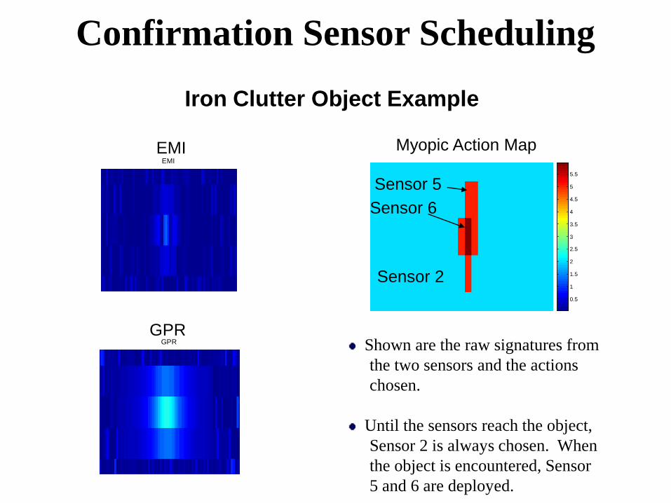
Myopic Action Map

Iron Clutter Object Example

Shown are the raw signatures fromthe two sensors and the actions chosen.

Until the sensors reach the object, Sensor 2 is always chosen. Whenthe object is encountered, Sensor5 and 6 are deployed.


1 2 3 4 5 6 7 8 9 100

0.5

1

Type

Pro

babi

lity

1 2 3 4 5 6 7 8 9 100

0.5

1

Type

Pro

babi

lity

1 2 3 4 5 6 7 8 9 100

0.5

1

Type

Pro

babi

lity

Initial Scanning Mode Confirmation

Active Sensing estimates the amount of “information gain” achievable from each of the 6 confirmation sensors. Information gain is a measureof the decreased entropy of the state PDF after making an observation.

Clutter objects (iron, aluminum, and non-metal) have been introduced to study false alarm rejection capabilities of algorithms.

Confirmation Sensor SchedulingIron Clutter Object Example

Confusion Matrix after Confirmation

2

56789

10

43

2 5 6 7 8 9 1043

1 0 0 0 0 0 0 0 0

0 1 0 0 0 0 0 0 0

0 0 1 0 0 0 0 0 0

0 0 0 0.7 0.3 0 0 0 0

0 0 0 0.2 0.8 0 0 0 0

0 0 0 0 0.2 0.8 0 0 0

0 0.1 0 0 0 0 0.9 0 0

0.1 0 0 0 0 0 0 0.9 0

0 0 0 0 0 0.2 0 0 0.8



1 - backgroundObject Types

Each Row Should Sum to One

• Sensors under development at Georgia Tech (Waymond Scott)• Data set used is the GATech “Three Sensor Dataset” (Feb.2004)

• Includes metal detector, radar, and seismic vibrometer.• Collection performed on three scenarios of mine/clutter arrangements.• Data used to guide sensor statistical simulations at U.Mich.

EMI SeismicGPR

Sensors from the Three Sensor Dataset

Downloadable Demo

Multiple Confirmation Sensor Scheduling

Optimal Policy

1D

1D

12D

123D

123D

1D

1D

1D1 – EMI

2 – GPR3 – SeismicD – Make Decision

Cltr1 – Hollow MetalCltr2 – Hollow Non-metalCltr3 – Non-hollow Non-metal

ResonanceLowLowMediumMediumMediumHighMediumMedium

Seismic

RCSLowHighHighHighMediumHighMediumHigh

DepthLowLowLowLowMediumHighMediumHigh

GPR

SizeLowLowLowMediumMediumHighHighHighSensor

ConductivityLowLowLowHighHighMediumHighHigh

EMI

DescriptionBkgCltr-3Cltr-2Cltr-1P-APP-ATM-APM-AT

Feature87654321

Object Type

Medium High

Medium Medium Medium

Low

High

Low

Low

Medium

Low

Assumptions: AT Mines Buried Deep, AP Mines Buried Very Shallow, et.al.

Always deploy three sensors

Always deploy best of two sensors: GPR + Seismic

Always deploy best single sensor: EMI

Suboptimal SM using best fixed sensor allocation

+ Optimal SM using weighted classifierreduction

Optimal sensor scheduling improves detection performance while reducing average dwell time.

Performance Comparison (Pc vs E[N])

+

+

++

+

+

+ Suboptimal SM using unweighted classifier

StatisticalContributions

l Marble,J., Blatt,D., Hero,A., ``Confirmation Sensor Scheduling using aReinforcement Learning Approach,'' SPIE: Detection and RemediationTechnologies for Mines and Minelike Targets XI, March 2006, Orlando, FL.

l Marble,J., Yagle,A., Hero,A, ``Sensor Management for Landmine Detection,''SPIE: Detection and Remediation Technologies for Mines and Minelike TargetsX, March 2005, Orlando, FL.

l Marble,J., Yagle,A., Hero,A, ``Multimodal, Adaptive Landmine Detection Using EMI and GPR,'' SPIE: Detection and Remediation Technologies for Mines and Minelike Targets X, March 2005, Orlando, FL.

ImagingSee-Through-Wall Radar

and Volumetric Landmine Imaging

l I.R.I.S. Adaptive Imagingl Iterative Redeployment of Imaging and Sensingl Adaptively build a large scene out of small aperture

radar measurements.l Use sensor scheduling to redeploy small aperture radar.

l Phase Delay Estimation and Correctionl Two methods proposed for homogeneous external walls.l The magic parameter: l Autofocus techniques required in real world system.

l Near Real Time Imaging of Large Scenesl 2D for STW and 3D for Landminel Matrix Implementation of Wavenumber Migrationl Development of a Forward Operator by “Reverse

Engineering” the Adjoint Operator

Imaging

2ετ

l SRI Sidelooking Radar

l Monostatic SARl Fully Polarimetric: HH, VV, HV

l Frequenciesl 800-2400 MHzl 301 Frequency Steps

l Antenna Height 7.5m

SRI International Building 409Menlo Park, CA

See-Through-Wall Radar Imaging

SRI International Building 409Menlo Park, CA

l SRI Sidelooking Radar

l Monostatic SARl Fully Polarimetric: HH, VV, HV

l Frequenciesl 800-2400 MHzl 301 Frequency Steps

l Antenna Height 7.5m

Azimuth, m

Ran

ge,

m

Wavefront Reconstruction

-20 -10 0 10 20

5

10

15

20

25

30

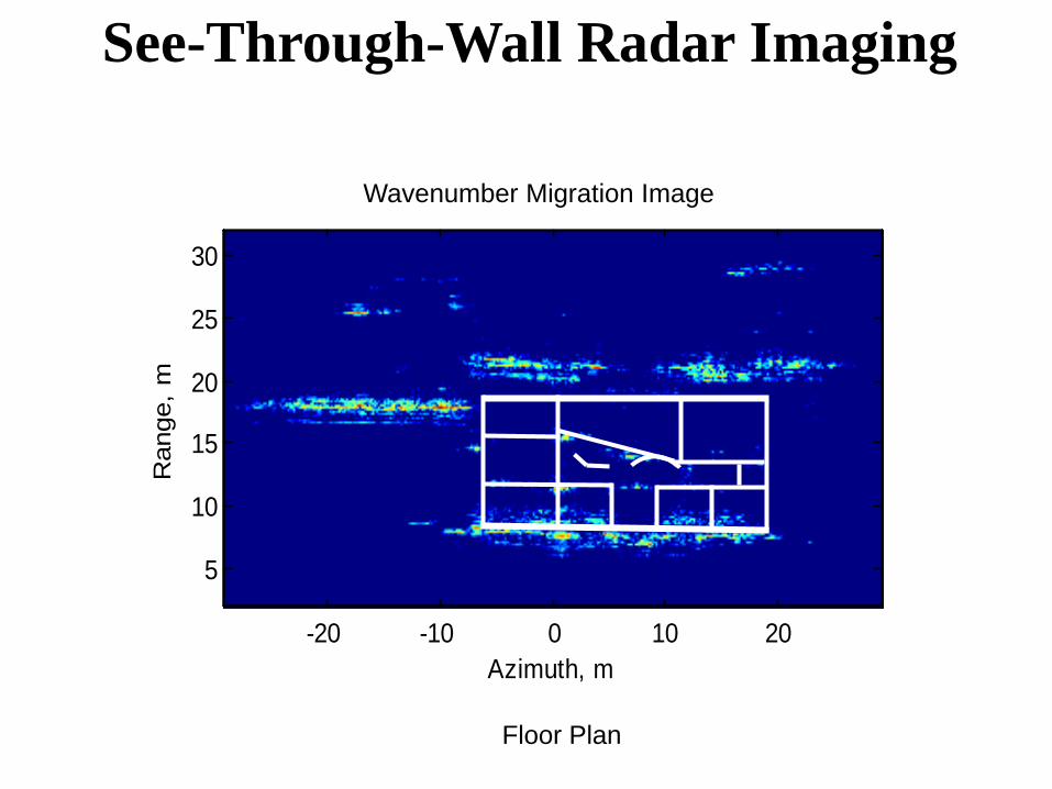
Wavenumber Migration Image


Synthetic Aperture, m

Rad

ial R

ange

, m

Filtered SAR Data

-20 -10 0 10 20

5

10

15

20

25

30

Raw Data

Azimuth, m

Ran

ge,

mWavefront Reconstruction

-20 -10 0 10 20

5

10

15

20

25

30



Azimuth, m

Ran

ge,

mWavefront Reconstruction

-20 -10 0 10 20

5

10

15

20

25

30



Floor Plan

Electric Field Energy Mapping

Down Range [m]

Cros

s Ra

nge

[m]

-25 -20 -15 -10 -5

-10

-5

0

5

10

Virtual Transmitter

Predict Information Gain(Energy or Resolution MAP)

Low Confidence Region

Uncertainty Map

Sensor IlluminationElements of the I.R.I.S. Strategy

Iterative Redeployment of Illumination and Sensing

ISAR Image

-4 -2 0 2 4

-4

-2

0

2

4

10 m

10 m10 m

10 m

Total Aperture: 40m

Observation

Dow

n R

ange

[m]

Cross Range [m]-5 0 5

-5

0

5

1

23 4

5

6

78

9

10

1112

Table

Chair

Sink

WeaponsCache

Empty Space Interior

Standard Scene

Total Aperture: 12*1m = 12m

l IRIS Simulation for Proof of Conceptl Bandwidth: 4-5GHzl Number Frequencies: 512l Aperture per side: 10ml Full Synthetic Array: 512 elementsl Subaperture Array: 50 elements

Full ISAR Image Adaptive IRIS Image

IRIS Simulation

IRIS “Modules”l Uncertainty Map – Inside Building

l The Ting Methodl The Yuan&Lin (inspired) Method

l Sensor Information Map – Outside Buildingl KL Divergence Metric (Max Info Gain)l Energy Method (Max SNR)

l Virtual Transmitterl Currently using “Enhanced Geometrical Optics”

l A high frequency approximation.l Mathematically simple and fastl Valid (and possibly only choice) at higher frequenciesl Not valid at corners

l Other Methods – Numerically Intensel All require 10 samples per (shortest) wavelengthl MoM, FEM, FDTD

l The Observationsl Simulated – Currently using Enhanced Geometrical Opticsl Real Data – Always best.

l Imagingl Sparse Reconstruction Based on Wavenumber Migrationl Other’s can be substituted based on performance characteristics.

Both Used in automated IRIS

Both Used

dtexerfx

t

t∫=−=

0

22)(π

Ting,M, Hero,A.O., “Sparse Image Reconstruction Using a Sparse Prior,” IEEE International Conference on Image Processing, Atlanta, GA, Oct. 8-11, 2006.

(Ting&Hero)

Confidence

Entropy

)(log)1()(log)( 22 pppppS −−−=

)|0( zIPp ==

Final uncertainty mapping (Map #1)

Uncertainty Map

Uncertainty Map

l Uncertainty Map shows pixels that are likely to be “empty”.

l Regions of the image that have not been viewed by the sensor are accounted forby the second Uncertainty Map. This second map isinspired by Yuan&Lin (JASA 2005).

l Note: Pixels are DirectionalMeaning that radar imagesare composed of directionalscatterers.

Most Uncertain

Region

First Iteration Map #1

Fifth Iteration Map #2

X

Dow

n R

ange [

m]

Cross Range [m]-5 0 5

-10

-5

0

5

10

Kullback Leibler Divergence – Information Gain

Virtual Transmitters

1 23

-Electric Field From Transmitter k.Observation Location

4 4.2 4.4 4.6 4.8 51

2

3

4

5

6

7

8

9 x 10-3E1 Electric Field Magnitude

Frequency [GHz]

Fiel

d St

reng

th

4 4.2 4.4 4.6 4.8 50

0.002

0.004

0.006

0.008

0.01

0.012E2 Electric Field Magnitude

Frequency [GHz]

Fiel

d St

reng

th

4 4.2 4.4 4.6 4.8 50

0.002

0.004

0.006

0.008

0.01E3 Electric Field Magnitude

Frequency [GHz]

Fiel

d St

reng

th

Div Map= Div(E1,E3)+ Div(E1,E2)

ReferenceField

HorizontalPerturbationField

VerticalPerturbationField

Div(Ek, Ej ) = log( )

Sensor Information Map

Rx

Tx

ObjectAir AirWall

Rs

Rt χ

χ’Rr

Virtual Transmitter

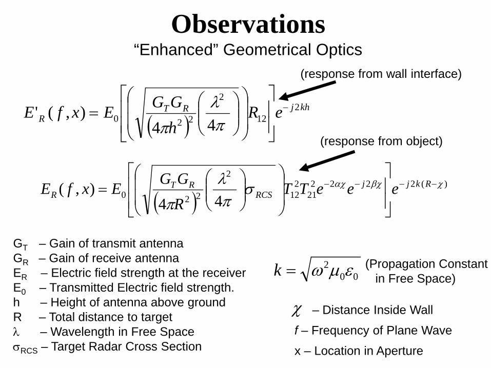
“Enhanced” Geometrical Optics

Observations

( )( ))(

2112223

2

0 4),( χβχαχσ

πλ −+−−−

= ts RRjkj

RCSts

RTR eeeTT

RRGGExfE

( )( )χβχαχ

πλ −−−−

= rRjkj

r

RTR eeeTT

RGGExfE 21122

2

0 ''4

),('

(Direct Path from Transmitter)

(response from object)

GT – Gain of transmit antennaGR – Gain of receive antennaER – Electric field strength at the receiver E0 – Transmitted Electric field strength.h – Height of antenna above groundd – Depth of target below the surfaceλ – Wavelength in Free SpaceσRCS – Target Radar Cross Section

002 εµω=k (Propagation Constant

in Free Space)

– Distance Inside Wallχ

x – Location in Aperture

f – Frequency of Plane Wave

Virtual Transmitter“Enhanced” Geometrical Optics

( ))(2222

212

12

2

220 44),( χβχαχσ

πλ

π−−−−

= Rkjj

RCSRT

R eeeTTRGGExfE

( )khjRT

R eRhGGExfE 2

12

2

220 44),(' −

=

πλ

π

(response from wall interface)

(response from object)

GT – Gain of transmit antennaGR – Gain of receive antennaER – Electric field strength at the receiver E0 – Transmitted Electric field strength.h – Height of antenna above groundR – Total distance to targetλ – Wavelength in Free SpaceσRCS – Target Radar Cross Section

002 εµω=k (Propagation Constant

in Free Space)

– Distance Inside Wallχ

x – Location in Aperture

f – Frequency of Plane Wave

Observations“Enhanced” Geometrical Optics

21

22

2

1121

−+=

ωεσµεωα

21

22

2

1121

++=

ωεσµεωβ

r

rR

ε

ε11

11

12

+

−

=

r

Tε+

=1

221

r

T

ε11

212

+=

rεµεωβ ≈Slightly

Conducting Media

Approximation

Fresnel Reflection andTransmission Coefficients

Attenuation and PropagationConstants in Conducting Media

“Enhanced” Geometrical Optics

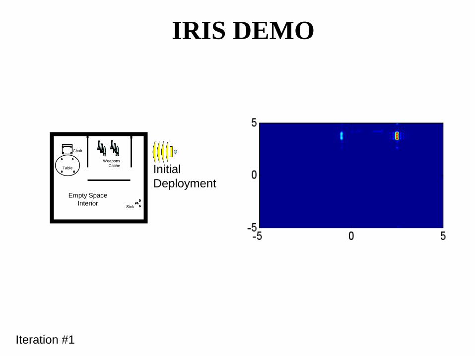
Table

Chair

Sink

WeaponsCache

Empty Space Interior

InitialDeployment

IRIS DEMO

Iteration #1

Iteration #2

IRIS DEMO

Iteration #3

IRIS DEMO

Iteration #4

IRIS DEMO

Iteration #5

IRIS DEMO

Iteration #6

IRIS DEMO

Iteration #7

IRIS DEMO

Iteration #8

IRIS DEMO

Iteration #9

IRIS DEMO

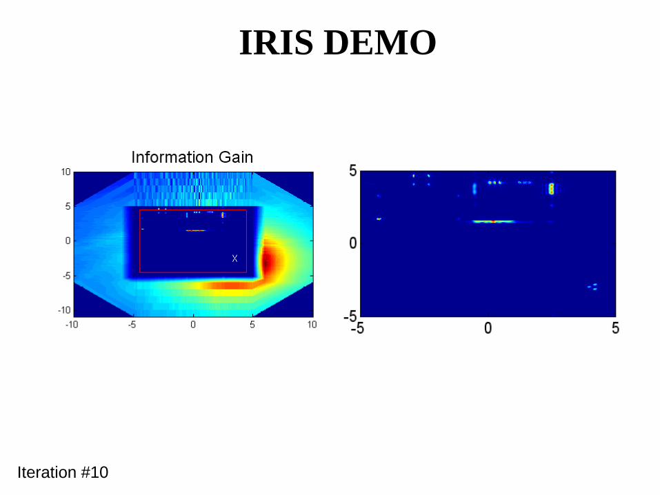
Iteration #10

IRIS DEMO

Iteration #11

IRIS DEMO

Iteration #12

IRIS DEMO

0 2 4 6 8 10 120

0.2

0.4

0.6

0.8

1D

etec

tion

Prob

abilit

y

Total Aperture [m]

CONVERGENCE

IRIS DEMO

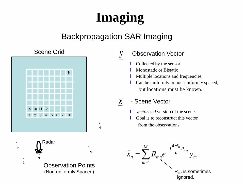
Backpropagation SAR Imaging

Scene Grid

1 2

N

3 4 5 6 7 8

9 10 11 12 . . .

y

x

- Observation Vector

- Scene Vector

l Collected by the sensorl Monostatic or Bistaticl Multiple locations and frequenciesl Can be uniformly or non-uniformly spaced,

but locations must be known.

l Vectorized version of the scene.l Goal is to reconstruct this vector

from the observations.

1

2

3

4

M

Radar

Observation Points(Non-uniformly Spaced)

∑=

+=

M

mm

Rcfj

mnn yeRx mn

1

4 0

ˆπ

Rmn is sometimesignored.

Imaging

l Looping (Desktop PC -2.2GHz, 2.0GBytes, 1-64bit - processor)l MATLAB 11 min 16 secl ANSI C: 1 min 1 sec

l Small Image (100 x 100 pixels) for discussion

l MATLAB (Matrix Multiplication – 1 processor)l Desktop PC (2.2GHz, 2.0GBytes, 1-64bit - processor) : OUT OF MEMORYl Lab PC (3.5GHz, 3.5GBytes, 1 processors): OUT OF MEMORYl Lab PC Linux (3.5GHz, 4GBytes, 1 processor): 1.7 sec l HPC (Linux Networx Evolocity II – 1 node): 2.7 sec

l MATLAB ( Matrix Multiplication Multithreading – 2 processors)l MAC (2GHz, 2GBytes, 2 processors) 1.05 secl Linux (3.5GHz, 4GBytes, 2 processors) 0.95 sec

100 pix

100 pix

l MATLAB ( FFT Acceleration)

l Wavenumber Migration (Multithreading - 2 processors) 0.09 sec

35x

1.8x

10x

Imaging

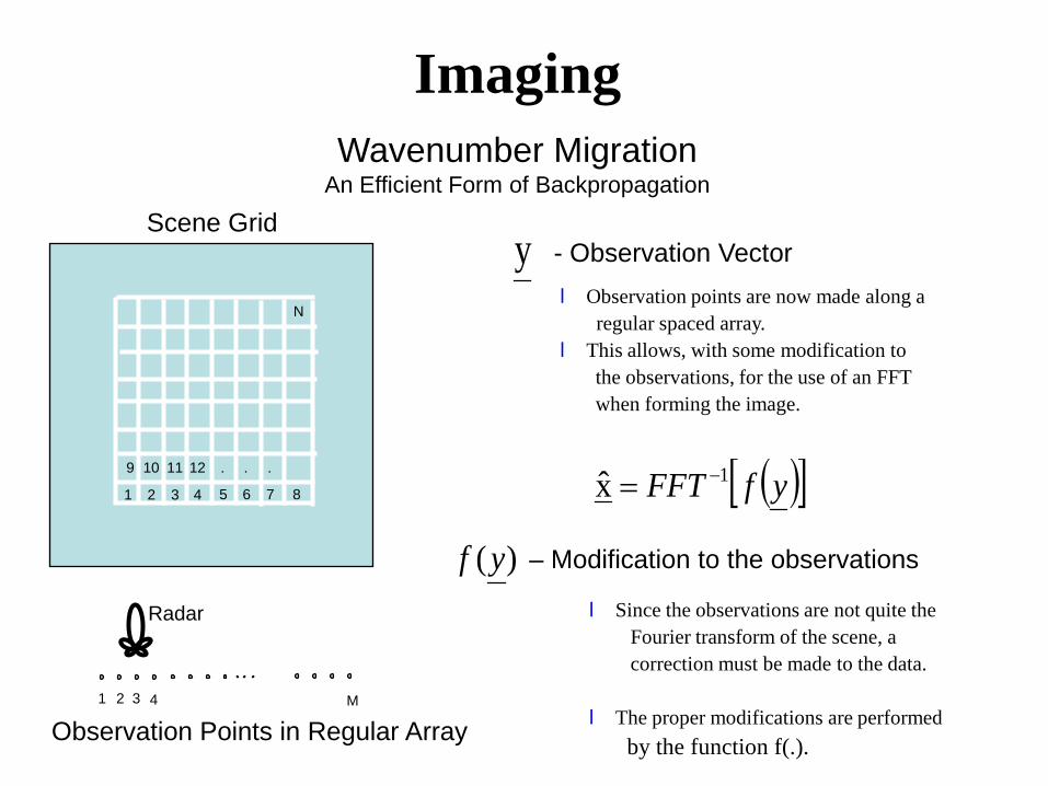
Wavenumber MigrationAn Efficient Form of Backpropagation

Scene Grid

1 2

N

3 4 5 6 7 8

9 10 11 12 . . .

y - Observation Vectorl Observation points are now made along a

regular spaced array.l This allows, with some modification to

the observations, for the use of an FFT when forming the image.

1 2 3 4 M

Radar

Observation Points in Regular Array

– Modification to the observations

l Since the observations are not quite theFourier transform of the scene, a correction must be made to the data.

l The proper modifications are performedby the function f(.).

( )[ ]yfFFT 1x −=

)(yf

Imaging

Azimuth

FFT

After Azimuth FFT

-60 -40 -20 0 20 40 60

30

40

50

60

70

80

After 2D Phase Compensation

-60 -40 -20 0 20 40 60

30

40

50

60

70

80

(Kx,Kz) Domain after Stolt Interpolation

-60 -40 -20 0 20 40 60

20

30

40

50

60

70

80

Focused Image

-1.5 -1 -0.5 0 0.5 1 1.5

-1.6

-1.4

-1.2

-1

-0.8

-0.6

-0.4

-0.2

0

0.2

0.4

2D

Phase

Comp

Stolt

Interp

2D

FFT

After Azimuth FFT

-60 -40 -20 0 20 40 60

30

40

50

60

70

80

After 2D Phase Compensation

-60 -40 -20 0 20 40 60

30

40

50

60

70

80

(Kx,Kz) Domain after Stolt Interpolation

-60 -40 -20 0 20 40 60

20

30

40

50

60

70

80

Mechanics ofWavenumber

Migration

Place in Ω-k

Format

2D Phase Comp.

StoltInterp.

2DFFT

PointSpreadFunction

FocusedPoint

R(kx,Ω) D(kx,kz)R(kx,Ω)F(kx,,Ω)

Imaging

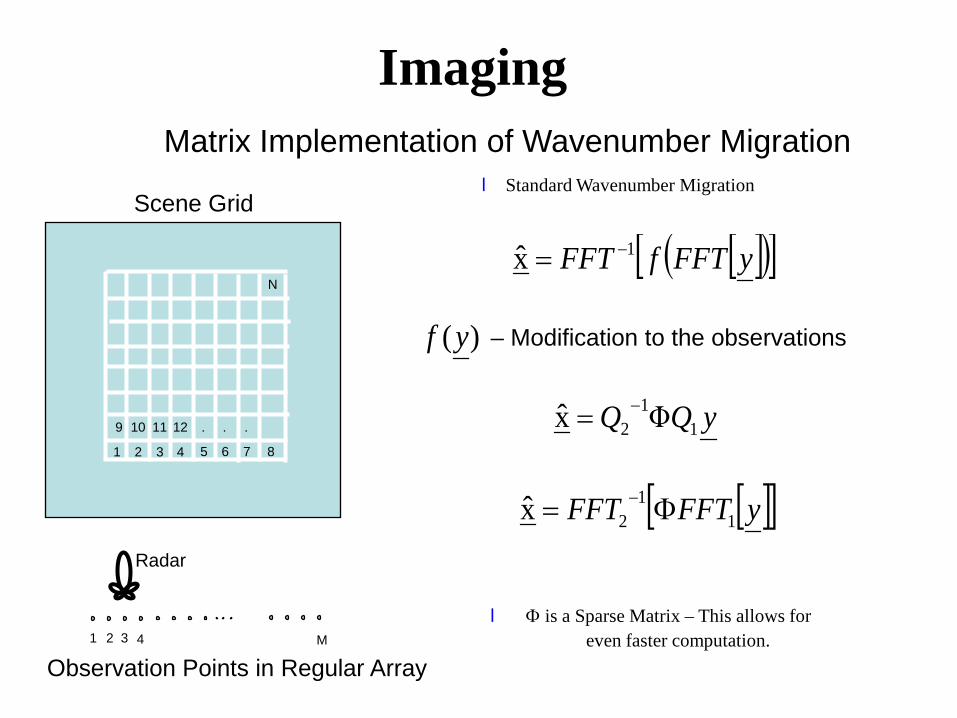
Scene Grid

1 2

N

3 4 5 6 7 8

9 10 11 12 . . .

1 2 3 4 M

Radar

Observation Points in Regular Array

– Modification to the observations

l Φ is a Sparse Matrix – This allows for even faster computation.

[ ]( )[ ]yFFTfFFT 1x −=

)(yf

Matrix Implementation of Wavenumber Migration

Imaging

l Standard Wavenumber Migration

yQQ 11

2 Φx −=

[ ][ ]yFFTFFT 11

2x Φ= −

SparsityModel

• Radar imagery often has a significant number of zero pixels.

• We want to make use of this fact to produce better reconstructions.

• A Sparsity Model for an image is proposed as an exponential distribution of pixel amplitudes combined with a discrete probability of zero.

Sparse Reconstruction

Image Pixel Amplitude

• This sparsity constraint cannot be implemented like the standardLagrange Multipliers.

0aexxfX ωδω +−= )()1()( || xa−

Imaging

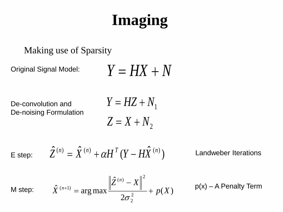
De-convolution andDe-noising Formulation

NHXY +=

2

1

NXZNHZY

+=+=

)ˆ(ˆˆ )()()( nTnn XHYHXZ −+= α

Original Signal Model:

E step: Landweber Iterations

Making use of Sparsity

)(2

ˆmaxargˆ

22

2)(

)1( XpXZ

Xn

n +−

=+

σM step: p(x) – A Penalty Term

Imaging

Pixel-wise Soft Threshold

M Step

)(2

ˆmaxargˆ

22

2)(

)1( XpXZ

Xn

n +−

=+

σM step:

Implementing a Sparsity Constraint

Soft Thresholding Implementation*

*M. Figueiredo and R. Novak, “An EM Algorithm forWavelet-based Image Restoration,” IEEE Trans. ImageProcessing, vol. 12, pp. 906-916, 2003.

)()1( ˆ nn ZX =+ ^

(Applied to Amplitude)

XXp λ=)(l1 penalty function

l0 penalty functionNumber of Non-zeropixels

Sparse Prior InformationAverage Number of Zero PixelsStatistical Distribution of Non-zero Pixels

M step:

Imaging

Forward Wavenumber Migration

Reverse Wavenumber Migration

Azimuth

FFT

2D

Phase

Comp

Stolt

Interp

2D

FFT

Place in Ω-k

Format

Phase Comp.

StoltInterp.

FFT-1

Azimuth

FFT

2D

Phase

Comp

Stolt

Interp

2D

FFTFFT InverseStolt

Phase(un)comp

Place inx-k

Format

ObservationDomain

ObservationDomain

ImageDomain

ImageDomain

)ˆ(ˆˆ )()()( nTnn XHYHXZ −+= α

(Imaging)

Efficient Landweber Iterations

(Un-imaging)

Imaging Un-Imaging

Imaging


-30 -20 -10 0 10 20 30-15

-10

-5

0

5

10

15

Imaging

3D Landmine Imaging

GPR Radar System

Dep

th [m

]

Along Track [m]

Sample Signature

-5 0 5

-0.2

-0.1

0

0.1

0.2

0.3

0.4

0.5

Depth: 2”

Dep

th [m

]

Along Track [m]

Sample Signature

-2 -1.5 -1 -0.5 0 0.5 1 1.5

0

0.05

0.1

0.15

0.2

0.25

0.3

0.35

0.4

0.45

Real WorldBounding Box

Want to determine:Object depth and sizeIn Three DimensionsIn Near Real Time

Diameter: 13”Height: 6”

Imaging

Imaging

Raw GPR Data

Imaging

Wavenumber Migration

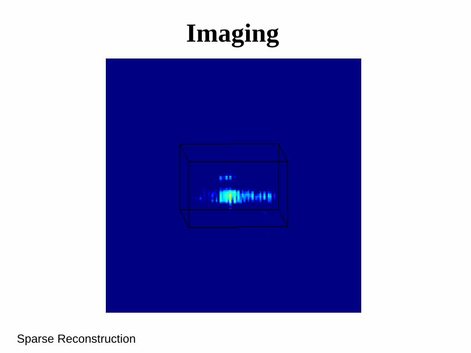
Imaging


ImagingContributions

l Marble,J.A., Hero,A.O., ``Iterative Redeployment of Illuminatiion andSensing (IRIS): Application to STW-SAR Imaging,'' in Proc. of the 25th Army Science Conference, Orlando, FL, Nov. 2006.

l Marble,J.A., Hero,A.O., ``Phase Distortion Correction for See-Through-The-Wall Imaging Radar,'' ICIP: International Conference on Image Processing 2006, Atlanta, GA, Oct. 2006.

l Marble,J., Hero,A, ``See Through The Wall Detection and Classification ofScattering Primitives,'' SPIE: Detection and Remediation Technologies forMines and Minelike Targets XI, March 2006, Orlando, FL.

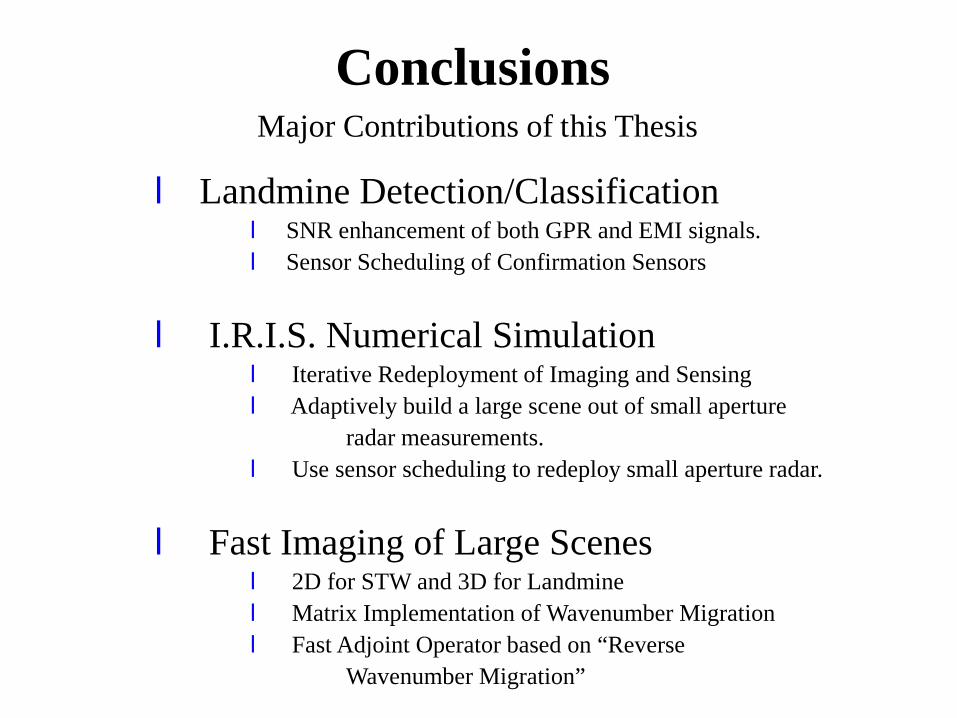
l Landmine Detection/Classification l SNR enhancement of both GPR and EMI signals.l Sensor Scheduling of Confirmation Sensors

l I.R.I.S. Numerical Simulationl Iterative Redeployment of Imaging and Sensingl Adaptively build a large scene out of small aperture

radar measurements.l Use sensor scheduling to redeploy small aperture radar.

l Fast Imaging of Large Scenesl 2D for STW and 3D for Landminel Matrix Implementation of Wavenumber Migrationl Fast Adjoint Operator based on “Reverse

Wavenumber Migration”

ConclusionsMajor Contributions of this Thesis

advances in surface penetrating technologies for …web.eecs.umich.edu/~aey/phd/marbles.pdf ·...

Documents