Advanced Physics Laboratory

Physics 370

Spring 2011

2

Instructor:

Name: Dr. Tom KirkmanOffice: PEngel 111 Phone: 363–3811 email: tkirkman@unix.csbsju.eduOffice Hour: 1:00 p.m. Day 4 Informal Office Hours: 7:30 a.m. – 5:30 p.m.

Texts:

• An Introduction to Error Analysisby John R Taylor (University Science, 1997)

• http://www.physics.csbsju.edu/370/

http://www.physics.csbsju.edu/stats/

Grading:

Your grade will be determined by averaging five scores: 3 lab scores, electronics workshopscore and paper score. Lab grades are based on what is recorded in your lab notebook.Please be complete and legible! You will probably need at least 2 of these notebooks (whichmay be “used”) as I’ll be grading old labs while you’ll working on current labs. Assignedwork is generally due at the beginning of the following class period. In particular your labnotebook must be turned in before the lab lecture for the following experiment. (If your labwork is incomplete, you may request an improved grade for a completed report, neverthelessturn in what you have!) All work (except the final version of your paper) contributing toyour grade must be turned in by our last meeting day: Friday April 29.

Questions:

There is no such thing as a dumb question. Questions asked during lecture or lab do not“interrupt”, rather they indicate your interests or misunderstandings. The aim of lab is todo things you’ve never done before; it’s no surprise if you’ve got questions.

Remember: you are almost never alone in your interests, your misunderstandings, or yourproblems. Please help your classmates and yourself by asking any question vaguely relatedto physics lab. If you don’t want to ask your question during class, that’s fine too: I canbe found almost any time on the 100-level floor of Engel Science Center. Ask if you don’tfind me, as I spend just as much time in the nearby labs as I do in my office.

Times/Locations:

Half of this course will be self-scheduled. I hope many of you will still choose to do that workin the scheduled slot, because you can be then sure to find me (i.e., help) at those timesand it will help you avoid the crime of procrastination. However, because of limited labequipment, in fact you cannot all perform the data collection simultaneously. Of course, dataanalysis (which usually takes much longer than data collection) can be done simultaneously.

4

Three cycles are scheduled for each lab. Most of the actual data collection and analysis willtake place in the suite of labs across from my office.

About a third of this course will meet at the scheduled time: lab lectures and electronicsworkshop. We will be using the astronomy lab room (PEngel 319) for lab lectures. Ifyou cannot attend at those times, the responsibility of mastering the material falls onyou. (An alternative class time—agreed to by all—would also be fine.) Note that lablectures typically run a bit more than an hour, which leaves plenty of time to start the labimmediately following the lab lecture. Groups will also need to schedule a night lab at theobservatory for photometry data collection.

“Do I have to do my lab work during the scheduled lab period?”

The answer is “No, but be forewarned:” it is not uncommon for students to earn Fs for thiscourse because they did not complete the required reports at the required time. While Iwill give some credit for late lab work, it is difficult and unpleasant (read: many fail!) toanalyze data that was collected a month ago. If you actually put in the scheduled four solidhours1 of lab work per cycle, I’ll work with you to make sure you complete labs on time.Again: the lab is scheduled for 1 p.m. to 5 p.m., if you fiddle around in lab and leave at3:30, you are doing half the required work and 50%=F.

Lab Notebook:

Your lab notebook is the primary, graded work-product for this course. It should representa detailed record of what you have done in the laboratory—complete enough so that youcould look back after a year or two and reconstruct your work just using your notebook andthis manual.

Your notebook should include your preparation for lab, sketches and diagrams to explainthe experiment, data collected, comments on difficulties, sample calculations, data analysis,final graphs, final results, answers to questions asked in the lab manual, and a critique ofthe lab. A list of suggested sections can be found in the 191 lab manual.

DO NOT collect data on scratch paper and then transfer to your notebook. Your notebookis to be a running record of what you have done, not a formal (all errors eliminated) report.You will write one formal lab report as the final project in this course. Do not delete, erase,or tear out sections of your notebook that you want to change. Instead, indicate in thenotebook what you want to change and why (such information can be valuable later on).Then lightly draw a line through the unwanted section and proceed with the new work.

Be Prepared!

In this “Advanced Lab” you will typically be combining some fairly advanced physics con-cepts with equally advanced instruments. The 10 minute pre-lab talk from 191/200 is

1i.e., hours when I’m immediately available to answer to your questions and not counting time spent oncomputer games, web browsing, waiting for your lab partner, etc.. . .

5

now stretched into an hour “lab lecture”; in a four hour “workshop” you will demonstrateyour ability to use the electrical instrumentation you spent a whole semester developing inPhysics 200. It will be quite easy to be overwhelmed by the theory and the instrumenta-tion. Your main defense against this tsunami of information is to read and understand thematerial before the lecture/lab. I know that this is difficult: technical readings never seemsto make sense the first time through. But frankly, one of the prime skills you should bedeveloping (i.e., the prime skill employers seek) is being able to read, understand, and acton technical documents. In 191 you were told: Read aggressively! Read with a pencil inhand so you can jot down questions, complete missing steps of algebra, and argue with theauthor. (In this case you can actually take your complaints, comments, and arguments tothe author, rather than imagining how the author would respond.) A significant problem isthat readings (in contrast to lectures) generally aim at getting the details right. But detailsobscure the big picture and misdirect attention. This leads to the suggestion of “skimming”the material. . . which is OK as long as that’s just the first step to understanding. I usuallystart by reading for detail, but bit-by-bit my confusion grows and I switch to skimming.But then I repeat the process from the start. After several repeats, I usually reach a pointwhere I’m not making progress, and I find I must do something more active like: talk tosomebody about the material, or try to solve a problem—perhaps one of my own design.The aim is to try to find out why the author thinks his points are the important ones.

Topics:

The following schedule is based on Day 1 labs.Equivalent labs occur on the following Day 2.

Day Date Topics

1/1 M Jan 17 Lab Lecture: Bubble Chambera

2/1 T Jan 253/1 W Feb 2

4/1 R Feb 10 Electrical Measurements Labb & Photometryc

5/1 F Feb 18 Lab Lecture: Thermionic Emission, Fortran, GPIB6/1 M Feb 287/1 T Mar 88/1 W Mar 23

9/1 R Mar 31 Lab Lecture: Langmuir Probe?d

10/1 F Apr 811/1 M Apr 18

12/1 F Apr 29 Draft of paper due

aRead “Systematic Error” and skim lab chapter before the lab lecture!bRead “Electrical Measurement Review” before the lab!cSchedule a night at the observatory!dOnly if photometry observations were impossible due to weather.

Paper: A stitch in time saves nine.

Presentation of a lab project as a paper is the final component of this course. While Iknow procrastination always seems like the easiest course, in fact, putting together a paper

6

months after you’ve completed the lab is time consuming. The easy course is actually tostart your paper (the figures particularly) soon after you’ve completed the lab. Productionof paper-quality figures immediately following the lab will save you a lot of time just whenyou most need it (at the end of the semester). Since this is your second try at writing apaper (you should have completed one for 332) I’ve provided only brief comments on thebasics: see page 133. More detailed information is available in the papers folder of theclass web site and the references listed on page 138. Paper topics will be assigned on a firstcome first served basis, so there is no reason to delay selecting your topic.

Contents

Systematic Error . . . . . . . . . . . . . . . . . . . . . . . . . . . . . . . . . . . . 9

Bubble Chamber . . . . . . . . . . . . . . . . . . . . . . . . . . . . . . . . . . . . 21

Photometry . . . . . . . . . . . . . . . . . . . . . . . . . . . . . . . . . . . . . . . 41

Electrical Measurements Review . . . . . . . . . . . . . . . . . . . . . . . . . . . 81

Electrical Measurements Lab . . . . . . . . . . . . . . . . . . . . . . . . . . . . . 97

Thermionic Emission . . . . . . . . . . . . . . . . . . . . . . . . . . . . . . . . . . 103

Scientific Paper . . . . . . . . . . . . . . . . . . . . . . . . . . . . . . . . . . . . . 133

Langmuir’s Probe . . . . . . . . . . . . . . . . . . . . . . . . . . . . . . . . . . . . 139

Appendix A: fit . . . . . . . . . . . . . . . . . . . . . . . . . . . . . . . . . . . . 171

Appendix B: plot . . . . . . . . . . . . . . . . . . . . . . . . . . . . . . . . . . . 177

Appendix C: fit & plot Example . . . . . . . . . . . . . . . . . . . . . . . . . . 183

Appendix D: Linux Commands . . . . . . . . . . . . . . . . . . . . . . . . . . . . 195

Appendix E: Error Formulae . . . . . . . . . . . . . . . . . . . . . . . . . . . . . 197

7

8 CONTENTS

0: Systematic Error

Physical scientists. . . know that measurements are never perfect and thus wantto know how true a given measurement is. This is a good practice, for it keepseveryone honest and prevents research reports from degenerating into fish stories.

Robert Laughlin (1998 Physics Nobel Laureate) p.10 A Different Universe

A hypothesis or theory is clear, decisive, and positive, but it is believed by noone but the man who created it. Experimental findings, on the other hand, aremessy, inexact things, which are believed by everyone except the man who didthe work.

Harlow Shapley, Through Rugged Ways to the Stars. 1969

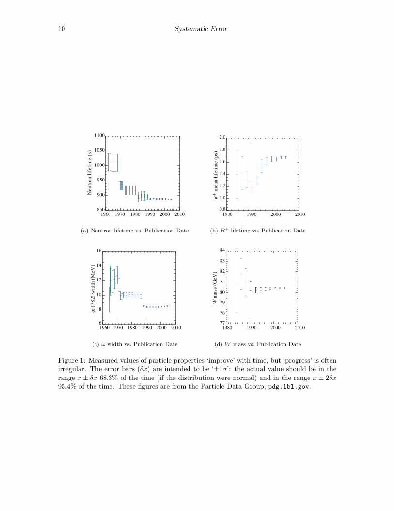
Perhaps the dullest possible presentation of progress1 in physics is displayed in Figure 1: themarch of improved experimental precision with time. The expected behavior is displayedin Figure 1(d): improved apparatus and better statistics (more measurements to average)results in steady uncertainty reduction with apparent convergence to a value consistent withany earlier measurement. However frequently (Figs. 1(a)–1(c)) the behavior shows a ‘final’value inconsistent with the early measurements. Setting aside the possibility of experimentalblunders, systematic error is almost certainly behind this ‘odd’ behavior. Uncertainties thatproduce different results on repeated measurement (sometimes called random errors) areeasy to detect (just repeat the measurement) and can perhaps be eliminated (the standarddeviation of the mean ∝ 1/N1/2 which as N → ∞, gets arbitrarily small). But systematicerrors do not telegraph their existence by producing varying results. Without any tell-tale signs, systematic errors can go undetected, much to the future embarrassment of theexperimenter. This semester you will be completing labs which display many of the problemsof non-random errors.

Experiment: Measuring Resistance I

Consider the case of the digital multimeter (DMM). Typically repeated measurement witha DMM produces exactly the same value—its random error is quite small. Of course,the absence of random error does not imply a perfect measurement; Calibration errors are

1Great advancements is physics (Newton, Maxwell, Einstein) were not much influenced by the quest formore sigfigs. Nevertheless, the ability to precisely control experiments is a measure of science’s reach andhistory clearly shows that discrepant experiments are a goad for improved theory.

9

10 Systematic Error

(a) Neutron lifetime vs. Publication Date (b) B+ lifetime vs. Publication Date

(c) ω width vs. Publication Date (d) W mass vs. Publication Date

Figure 1: Measured values of particle properties ‘improve’ with time, but ‘progress’ is oftenirregular. The error bars (δx) are intended to be ‘±1σ’: the actual value should be in therange x± δx 68.3% of the time (if the distribution were normal) and in the range x± 2δx95.4% of the time. These figures are from the Particle Data Group, pdg.lbl.gov.

Systematic Error 11

–10 –5 0 5 10

2

1

0

–1

–2

Voltage (V)

Cur

rent

(m

A)

A

VRpowersupply

V δV I δI(V) (V) (mA) (mA)

0.9964 .005 0.2002 .0012.984 .007 0.6005 .0034.973 .009 1.0007 .0056.963 .011 1.4010 .0078.953 .013 1.8009 .009

10.942 .015 2.211 .012−0.9962 .005 −0.1996 .001−2.980 .007 −0.6000 .003−4.969 .009 −1.0002 .005−6.959 .011 −1.4004 .007−8.948 .013 −1.8001 .009−10.938 .015 −2.206 .012

Figure 2: A pair DM-441B DMMs were used to measure the voltage across (V ) and thecurrent through (I) a 4.99 kΩ resistor

expected and reported in the device’s specifications. Using a pair of DM-441B multimeters,I measured the current through and the voltage across a resistor. (The circuit and resultsare displayed in Figure 2.) Fitting the expected linear relationship (I = V/R), Linfitreported R = 4.9696± .0016 kΩ (i.e., a relative error of 0.03%) with a reduced χ2 of .11. (Agraphical display showing all the following resistance measurements appears in Figure 3. Itlooks quite similar to the results reported in Figs. 1.)

This result is wrong and/or misleading. The small reduced χ2 correctly flags the fact thatthe observed deviation of the data from the fit is much less than what should have resultedfrom the supplied uncertainties in V and I (which were calculated from the manufacturer’sspecifications). Apparently the deviation between the actual voltage and the measuredvoltage does not fluctuate irregularly, rather there is a high degree of consistency of theform:

Vactual = a+ bVmeasured (1)

where a is small and b ≈ 1. This is exactly the sort of behavior expected with calibrationerrors. Using the manufacturer’s specifications (essentially δV/V ≈ .001 and δI/I ≈ .005)we would expect any resistance calculated by V/I to have a relative error of

√.12 + .52 =

.51% (i.e., an absolute error of ±.025 kΩ for this resistor) whereas Linfit reported an error17 times smaller. (If the errors were unbiased and random, Linfit could properly reportsome error reduction due to “averaging:” using all N = 12 data points—perhaps an errorreduction by a factor of N1/2 ≈ 3.5—but not by a factor of 17.) Linfit has ignored thesystematic error that was entered and is basing its error estimate just on the deviationbetween data and fit. (Do notice that Linfit warned of this problem when it noted the smallreduced χ2.)

12 Systematic Error

A B C

4.985

4.980

4.975

4.970

Res

ista

nce

(k

A B C

4.99

4.98

4.97

4.96

4.95

Ω)

Figure 3: Three different experiments are used to determine resistance: (A) a pair of DM-441B: V/I, (B) a pair of Keithley 6-digit DMM: V/I, (C) a Keithley 6-digit DMM directR. The left plot displays the results with error bars determined from Linfit; the right plotdisplays errors calculated using each device’s specifications. Note that according to Linfiterrors the measurements are inconsistent whereas they are consistent using the error directlycalculated using each device’s specifications.

When the experiment was repeated with 6-digit meters, the result was R = 4.9828 ±.0001 kΩ with a reduced χ2 of .03. (So calibration errors were again a problem and the twomeasurements of R are inconsistent.) Direct application of the manufacturer’s specificationsto a V/I calculation produced a 30× larger error: ±.003 kΩ

A direct measurement of R with a third 6-digit DMM, resulted in R = 4.9845 ± .0006 kΩ.

Notice that if Linfit errors are reported as accurate I will be embarrassed by future measure-ments which will point out the inconsistency. On the other hand direct use of calibrationerrors produces no inconsistency. (The graphical display in Figure 3 of these numericalresults is clearly the best way to appreciate the problem.) How can we know in advancewhich errors to report? Reduced χ2 much greater or much less than one is always a signalthat there is a problem with the fit (and particularly with any reported error).

Lesson: Fitting programs are designed with random error in mind and hence do not prop-erly include systematic errors. When systematic errors dominate random errors, computerreported ‘errors’ are some sort of nonsense.

Comment: If a high precision resistance measurement is required there is no substitutefor making sure that when the DMM reads 1.00000 V the actual voltage is also 1.00000 V.Calibration services exist to periodically (typically annually) check that the meters readtrue. (However, our SJU DMMs are not calibrated periodically.)

Warning: Statistics seems to suggest that arbitrarily small uncertainties can be obtainedsimply by taking more data. (Parameter uncertainties, like the standard deviation of the

Systematic Error 13

mean, will approach zero in proportion to the inverse square-root of the number of datapoints.) This promise of asymptotic perfection is based on the assumption that errors areexactly unbiased — so that with a large number of data points the errors will cancel and theunderlying actual mean behavior will be revealed. However, in real experiments the errorsare almost never unbiased; systematic errors cannot generally be removed by averaging.Care is always required in interpreting computer reported uncertainties. You must alwaysuse your judgment to decide if your equipment really has the ability to determine theparameters to accuracy suggested by computer analysis. You should particularly be onyour guard when large datasets have resulted in errors much smaller than those reportedfor the individual data points.

Measure Twice: Systematic Error’s Bane

In the thermionic emission lab you will measure how various properties of a hot tungstenwire are affected by its temperature. The presence of some problem with the thermionic labmeasurements is revealed by the odd reduced χ2 in fits, but how can we determine whichmeasurements are the source of the problem? Systematic errors are most commonly foundby measuring the same quantity using two different methods and not getting the same result.(And this will be the approach in this course: you will often be asked to measure a quantity(e.g., path length, temperature, plasma number density) using two different methods, andfind different answers.) Under these circumstances we can use the deviation between thetwo different measurements as an estimate for the systematic error. (Of course, the errorcould also be even larger than this estimate!)

Problem of Definition

Often experiments require judgment. The required judgments often seem insignificant: Isthis the peak of the resonance curve? Is A now lined up with B? Is the image now best infocus? Is this the start and end of one fringe? While it may seem that anyone would makethe same judgments, history has shown that often such judgments contain small observerbiases. “Problem of definition errors” are errors associated with such judgments.

Historical Aside: The “personal equation” and the standard deviation of the mean.

Historically the first attempts at precision measurement were in astrometry (accurate mea-surement of positions in the sky) and geodesy (accurate measurement of positions on Earth).In both cases the simplest possible measurement was required: lining up an object of interestwith a crosshair and recording the data point. By repeatedly making these measurements,the mean position was very accurately determined. (The standard deviation of the meanis the standard deviation of the measurements divided by the square root of the numberof measurements. So averaging 100 measurements allowed the error to be reduced by afactor of 10.) It was slowly (and painfully: people were fired for being ‘poor’ observers)determined that even as simple an observation as lining up A and B was seen differently bydifferent people. Astronomers call this the “personal equation”: an extra adjustment to bemade to an observer’s measurements to be consistent with other observers’ measurements.This small bias would never have been noticed without the error-reduction produced by

14 Systematic Error

averaging. Do notice that in this case the mean value was not the ‘correct’ value: the per-sonal equation was needed to remove unconscious biases. Any time you use the standarddeviation of the mean to substantially reduce error, you must be sure that the randomcomponent you seek to remove is exactly unbiased, that is the mean answer is the correctanswer.

In the bubble chamber lab, you will make path-length measurements from which you willdetermine a particle’s mass. Length measurements (like any measurement) are subject toerror, say 0.1 mm. A computer will actually calculate the distance, but you have to judge(and mark) the beginning and end of the paths. The resulting error is a combination ofinstrument errors and judgment errors (problem of definition errors). Both of these errorshave a random component and a systematic component (calibration errors for the machine,unconscious bias in your judgments). A relatively unsophisticated statistical treatment ofthese length measurements produces a rather large uncertainty in the average path length(and hence in the particle’s mass calculated from this length). However, a more sophisticatedtreatment of the same length data produces an incredibly small estimated length errormuch less than 0.1 mm. Of course it’s the aim of fancy methods to give ‘more bangfor the buck’ (i.e., smaller errors for the same inputs), however no amount of statisticalmanipulation can remove built in biases, which act just like systematic (non-fluctuating)calibration errors. Personal choices about the exact location of path-beginning and path-endwill bias length measurements, so while random length errors can be reduced by averaging(or fancy statistical methods), the silent systematic errors will remain.

Experiment: Measuring Resistance II

If the maximum applied voltage in the resistance experiment is increased from ±10 V to±40 V a new problem arises. The reduced χ2 for a linear fit balloons by a factor of about 50.The problem here is that our simple model for the resistor I = V/R (where R is a constant)ignores the dependence of resistance on temperature. At the extremes of voltage (±40 V)about 1

3 W of heat is being dumped into the resistor: it will not remain at room temperature.If we modify the model of a resistor to include power’s influence on temperature and henceon resistance, say:

I =V

k1(1 + k2V 2)(2)

(where fitting constant k1 represents the room temperature resistance and k2 is a factorallowing the electrical power dissipated in the resistor to influence that resistance), wereturn to the (too small) value of reduced χ2 seen with linear fits to lower voltage data.However even with this fix it is found that the fit parameters depend on the order the datais taken. Because of ‘thermal inertia’ the temperature (and hence the resistance) of theresistor will lag the t → ∞ temperature: T will be a bit low if the resistor is heating upduring data collection or a bit high if the resistor is cooling down. The amount of this lagwill depend on the amount of time the resistor is allowed to equilibrate to a new appliedvoltage. Dependence of data on history (order of data collection) is called hysteresis.

You might guess that the solution to this ‘problem’ is to always use the most accurate modelof the system under study. However it is known that that resistance of resistors depends onpressure, magnetic field, ambient radiation, and its history of exposure to these quantities.Very commonly we simply don’t care about things at this level of detail and seek the fewest

Systematic Error 15

possible parameters to ‘adequately’ describe the system. A resistor subjected to extremes ofvoltage does not actually have a resistance. Nevertheless that single number does go a longway in describing the resistor. With luck, the fit parameters of a too-simple model have someresemblance to reality. In the case of our Ohm’s law resistance experiment, the resultingvalue is something of an average of the high and low temperature resistances. However, it isunlikely that the computer-reported error in a fit parameter has any significant connectionto reality (like the difference between the high and low temperature resistances) since theerror will depend on the number of data points used.

The quote often attributed2 to Einstein: “things should be made as simple as possible,but not simpler” I hope makes clear that part of art of physics is to recognize the fruitfulsimplifications.

Lesson: We are always fitting less-than-perfect theories to less-than-perfect data. Themeaning of of the resulting parameters (and certainly the error in those parameters) isnever immediately clear: judgment is almost always required.

The Spherical Cow

I conceive that the chief aim of the physicist in discussing a theoretical problemis to obtain ‘insight’ — to see which of the numerous factors are particularlyconcerned in any effect and how they work together to give it. For this purposea legitimate approximation is not just an unavoidable evil; it is a discernmentthat certain factors — certain complications of the problem — do not contributeappreciably to the result. We satisfy ourselves that they may be left aside; andthe mechanism stands out more clearly freed from these irrelevancies. Thisdiscernment is only a continuation of a task begun by the physicist before themathematical premises of the problem could even be stated; for in any naturalproblem the actual conditions are of extreme complexity and the first step is toselect those which have an essential influence on the result — in short, to gethold of the right end of the stick.

A. S. Eddington, The Internal Constitution of the Stars, 1926, pp 101–2

As Eddington states above, the real world is filled with an infinity of details which a priorimight affect an experimental outcome (e.g., the phase of the Moon). If the infinity of detailsare all equally important, science cannot proceed. Science’s hope is that a beginning maybe made by striping out as much of that detail as possible (‘simple as possible’). If theresulting model behaves —at least a little bit— like the real world, we may have a hold onthe right end of the stick.

The short hand name for a too-simple model is a “spherical cow” (yes there is even a bookwith that title: Clemens QH541.15.M34 1985). The name comes from a joke that everyphysicist is required to learn:

Ever lower milk prices force a Wisconsin dairy farmer to try desperate—even

2“The supreme goal of all theory is to make the irreducible basic elements as simple and as few as possiblewithout having to surrender the adequate representation of a single datum of experience” p.9 On the Method

of Theoretical Physics is an actual Einstein quote, if not as pithy—or simple.

16 Systematic Error

crazy—methods to improve milk production. At he end of his rope, he drivesto Madison to consult with the greatest seer available: a theoretical physicist.The physicist listens to him, asks a few questions, and then says he’ll take theassignment, and that it will take only a few hours to solve the problem. Afew weeks later, the physicist phones the farmer, and says “I’ve got the answer.The solution turned out to be a bit more complicated than I thought and I’mpresenting it at this afternoon’s Theory Seminar”. At the seminar the farmerfinds a handful of people drinking tea and munching on cookies—none of whomlooks like a farmer. As the talk begins the physicist approaches the blackboardand draws a big circle. “First, we assume a spherical cow...” (Yes that is thepunch line)

One hopes (as in the spherical cow story) that approximations are clearly reported inderivations. Indeed, many of the ‘problems’ you’ll face this semester stem from using highaccuracy test equipment to test an approximate theory. (It may be helpful to recall the191 lab on measuring the kinetic coefficient of friction in which you found that accuratemeasurement invalidated F = µkN where µk was a constant. Nevertheless ‘coefficient offriction’ is a useful approximation.)

For example, in the Langmuir’s probe lab we assume that the plasma is in thermal equi-librium, i.e., that the electrons follow the Maxwell-Boltzmann speed distribution and makea host of additional approximations that, when tested, turn out to be not exactly true. Inthat lab, you will find an explicit discussion of the error (20% !) in the theoretical equationEq. 7.53.

Ji ≈1

2en∞

√

kTeMi

(3)

Again this ‘error’ is not a result of a measurement, but simply a report that if the theoryis done with slightly different simplifications, different equations result. Only rarely areerrors reported in theoretical results, but they almost always have them! (Use of flawed orapproximate parameters is actually quite common, particularly in engineering and processcontrol—where consistent conditions rather than fundamental parameters are the mainconcern.)

What can be done when the model seems to produce a useful, but statistically invalid fitto the data?

0. Use it! Perhaps the deviations are insignificant for the engineering problem at hand,in which case you may not care to explore the reasons for the ‘small’ (compared towhat matters) deviations, and instead use the model as a ‘good enough’ approximationto reality.

1. Find a model that works. This obvious solution is always the best solution, butoften (as in these labs) not a practical solution, given the constraints.

2. Monte Carlo simulation of the experiment. If you fully understand the processesgoing on in the experiment, you can perhaps simulate the entire process on a computer:the computer simulates the experimental apparatus, producing simulated data setswhich can be analyzed using the flawed model. One can detect differences (biasesand/or random fluctuation) between the fit parameters and the ‘actual’ values (whichare known because they are set inside the computer program).

Systematic Error 17

3. Repeat the experiment and report the fluctuation of the fit parameters.In some sense the reporting of parameter errors is damage control: you can only belabeled a fraud and a cheat if, when reproducing your work, folks find results outsideof the ballpark you specify. You can play it safe by redoing the experiment yourselfand finding the likely range (standard deviation) of variation in fit parameters. Inthis case one wants to be careful to state that parameter values are being reported notphysical parameters (e.g., ‘indicated temperature’ rather than actual temperature).Again, since systematic errors do not result in fluctuation, the likely deviation betweenthe physical parameters and the fit parameters is not known. This was the approachused in the 191 µk experiment.

4. Use bootstrapping3 to simulate multiple actual experiments. Bootstrapping‘resamples’ (i.e., takes subsets) from the one in-hand data set, and subjects thesesubsets to the same fitting procedure. Variation in the fit parameters can then bereported as bootstrap estimates of parameter variation. The program fit can boot-strap. (Again: report that an unknown amount of systematic error is likely to bepresent.)

5. Fudge the data.

In dire circumstances, you might try scaling all your x and y error bars by aconstant factor until the probability is acceptable (0.5, say), to get plausiblevalues for σA and σB .

Numerical Recipes by Press, et al., 3rd ed. p. 787

Increase the size of your error bars so you get reduced χ2 = 1, and then calculateerrors as in the usual approach. Clearly this is the least legitimate procedure (but itis what LINFIT does). One must warn readers of the dicey nature of the resultingerror estimates. The program fit can fudge.

Special Problem: Temperature

Measuring temperature is a particular problem. (This semester you’ll do two labs thatinvolve measuring temperatures above 1000 K in situations a bit removed from the experi-menter.) You may remember from 211 that while temperature is a common part of humanexperience, it has a strikingly abstruse definition:

1

kT≡ ∂ ln Ω

∂E(4)

While the usual properties of Newtonian physics (mass, position, velocity, etc.) exist at anytime, temperature is a property that exists contingent on a situation: ‘thermal equilibrium’.And thermal equilibrium is an idealization only approximately achieved—never exactlyachieved—in real life. Furthermore in these experiments, thermal equilibrium is not evenclosely approximated, so the resulting temperatures have somewhat restricted meanings.

In the photometry lab ‘the temperature of stars’ is measured. In fact stars do not have atemperature and are not in thermal equilibrium. Nevertheless, astronomers find it useful todefine an ‘effective temperature’ which is really just a fit parameter that is adjusted for thebest match between the light produced by the star and the light predicted by the model.

3wiki Bootstrapping (statistics)

18 Systematic Error

Special Problem: Assuming Away Variation

In the 191 µk lab, you assumed the sliding motion was characterized by one value of µk,whereas a little experimentation finds usually slippery and sticky locations (handprints?). Inthe thermionic emission lab you will measure how various properties of a hot wire depend ontemperature, however the hot wire does not actually have a temperature: near the supportsthe wire is cooled by those supports and hence is at a lower temperature. Our spherical cowmodels have simplified away actual variation. The hope is that the fit model will threadbetween the extremes and find something like the typical value. Of course, real variationswill result in deviations-from-fit which will be detected if sufficiently accurate measurementsare made.

Special Problem: Derive in Idealized Geometry, Measure in Real Geometry

Often results are derived in simplified geometry: perfect spheres, infinite cylinders, flatplanes, whereas measurements are made in this imperfect world. In these labs (and often inreal life) these complications are set aside; instead of waiting for perfect theory, experimentcan test if we have “the right end of the stick”. Thus a Spherical Cow is born. The theoryshould of course be re-done using the actual geometry, but often such calculations areextremely complex. Engineering can often proceed perfectly adequately with such a firstapproximation (with due allowance for a safety factor) and, practically speaking, we simplymay not need accuracy beyond a certain number of sigfigs. Indeed it takes a special breedof physicist to push for the next sigfig; such folks are often found in national standards labslike nist.gov.

Special Problem: Transducer Calibration

High precision measurement is most commonly electrical in nature: voltmeters, frequencycounters, etc.. . . Transducers are devices that convert a quantity of interest (e.g., pressure,temperature, light intensity) into an electrical quantity for precise measurement. The for-mula that relates the measured electrical quantity back to the quantity-of-interest is called acalibration. Commonly the uncertainty in calibration vastly exceeds the uncertainty in theelectrical measuring device. Thus the error in, say, pressure δP has nothing to do with theerror in, say, the voltmeter δV . This can come about for a variety of reasons. For example,the calibration may assume that there is a simple single-variable relationship between Pand V (P = f(V )), whereas in fact there may be an uncontrolled second variable involved(as in P = f(V,X)). Uncontrolled variations in X produce mis-calculated P . Commonly acomplex relationship between the quantities has been over-simplified by choice of a simpleformula relating the quantities. In this case the error will be systematic as actual P will besystematically above or below the value calculated from V using the formula.

The Fit Elephant

I remember a public lecture in the late 1970s by the theoretical astrophysicist Don Cox, inwhich he said

Systematic Error 19

Give me one free parameter and I’ll give you an elephant. Give me two and I’llmake it wag its tail

Cox was certainly not the originator4 of this sort of statement, for example, Freeman Dysonwrites5 that in 1953 Enrico Fermi quoted Johnny von Neumann as saying:

with four parameters I can fit an elephant and with five I can make him wigglehis trunk

The fit elephant is the opposite of the spherical cow: totally unconstrained parameters areadded willy-nilly to the model in order to chase the data. The parameter k2 in the hotresistor equation (Eq. 2) is potentially such a dangerously free parameter: I will accept anyvalue the computer suggests if only it improves the fit. While I have provided a story whichsuggests why such a term might be present, I have not actually checked that there is anytruth in the story (for example, by measuring the actual temperature of the resistor at highvoltage and by measuring the resistance of the resistor when placed in an oven). Skepticismabout such inventions is expressed as Occam’s razor6 and the law of parsimony.

Purpose:

In all your physics labs we have stressed the importance of ‘error analysis’. However, inthis course you will have little use for that form of error analysis (because it was basedon computer reports of random errors). Instead, my aim in this course is to introduceyou to the problems of non-random error. In the bubble chamber lab you will see howincreasingly sophisticated analysis can reveal systematic error not important or evidentin more elementary analysis. In the other labs you will see how systematic error can berevealed by measuring the same quantity using different methods. In all of these labs youwill use too simple theory to extract characterizing parameters, which are not exactly thesame quantity as might occur in a perfect version of the problem.

Comment:

The lesson: “measure twice using different methods” is often impractical in real life. Thereal message is to be constantly aware that the numbers displayed on the meter may notbe the truth. Be vigilant; check calibrations and assumptions whenever you can. But theopening Shapley quotation tells the truth: “Experimental findings. . . are messy, inexactthings, which are believed by everyone except the man who did the work”.

4Brown & Sethna, Phys.Rev.E, 68 021904 (2003), reports attributions to C.F. Gauss, Niels Bohr, LordKelvin, Enrico Fermi, and Richard Feynman; I would add Eugene Wigner. The first Google Books hit is in1959.

5Nature 427, 297 (2004), Mayer, el al., Am. J. Phys. 78, 648 (2010), found the required 4+1 (complex)parameters

6“entia non sunt multiplicanda praeter necessitatem”, roughly (Wiki) translated as “entities must not bemultiplied beyond necessity”.

20 Systematic Error

1: Bubble Chamber

Purpose

The purpose of this experiment is to determine the rest mass of the pion (mπ) and the restmass of the muon (mµ).

Introduction

Particle physics (a.k.a. high energy physics) is the division of physics which investigatesthe behavior of particles involved in “high” energy collisions. (“High” here means energiesgreater than those found in nuclear reactions, i.e., more than 100 MeV=0.1 GeV. Thehighest energy particle accelerators available today produce collisions with energies of a fewmillion MeV = TeV.)

The first “new” particles discovered (circa 1940) by particle physicists were the pion (π)and the muon (µ). In spite of roughly similar masses (near 100 MeV, compare: electronmass = .511 MeV and proton mass = 938 MeV), these two particles have quite differentproperties.

The muon is a relative of the electron (and hence is called a lepton). It comes in particle(µ−) and anti-particle (µ+) versions and has spin 1

2 . Unlike the electron, the muon isunstable. It decays into two neutrinos (ν) and an electron (or positron) after a mean life of2× 10−6 s:

µ+ −→ ν + ν + e+ (1.1)

µ− −→ ν + ν + e− (1.2)

The pion belongs to the class of particles called mesons. Unlike leptons, mesons interactwith protons and neutrons through an additional force called the strong nuclear force (a.k.a.,color force). (Particles that can feel this force are called hadrons.) Unlike leptons, mesonsare known to be composite particles: each is made of a quark and an antiquark. The pioncomes in three versions: π+, π0, and π− and has spin 0. All the pions are unstable; the π+

decays after a mean life of 3× 10−8 s:

π+ −→ µ+ + ν. (1.3)

(The π0 has a slightly smaller mass and decays much faster than the π±. It is not seen inthis experiment.)

21

22 Bubble Chamber

Particle Detection

Since the particles studied by particle physics are sub microscopic and decay “quickly”,particle detection is a problem. Most existing particle detectors rely on the fact that as acharged particle moves by an electron (e.g., an electron in an atom of the material throughwhich the charged particle is moving), the electron feels a net impulse. If the charged particlecomes close enough to the electron and/or is moving slowly enough (so the interaction is longenough), the impulse on the electron will be sufficient to eject the electron from its atom,producing a free electron and an ion. Thus a charged particle moving through materialleaves a trail of ions. This trail can be detected in many ways (e.g., by direct electronicmeans as in a modern wire chamber or chemically as when the material is a photographicplate or emulsion). In this experiment the ion trail is made visible by vapor bubbles whichare seeded by individual ions in boiling material (here liquid hydrogen). The bubbles arelarge enough to be photographed whereas the ion trail itself is much too narrow.

Relativistic Kinematics

Recall the following from Modern Physics:

E = γmc2 (1.4)

T ≡ E −mc2 (1.5)

pc = γmvc = γmc2β = Eβ (1.6)

E2 − (pc)2 =[

γmc2]2 (

1− β2)

=[

mc2]2

(1.7)

where:

β = v/c (1.8)

γ =1

√

1− β2(1.9)

and v is the velocity of the particle with rest mass m, momentum p, total energy E andkinetic energy T . Note that E, T , pc, and mc2 all have the dimensions of energy; it iscustomary to express each in MeV and even say “the momentum of the particle is 5 MeV”or “the mass of the particle is 938 MeV.” (Of course, technically the momentum of theparticle would be 5 MeV/c and the mass 938 MeV/c2. Basically what we are doing isredefining “momentum” to be pc and “mass” to be mc2. Since the “c” has disappeared,this re-naming is sometimes called “setting c = 1”.)

For future reference, note from Equation 1.6 that if β → 1, E ≈ pc and from Equation 1.7that if m = 0, E = pc. Of course, massless particles (like light) must travel at the speed oflight (i.e., β = 1).

Momentum Measurements

Classically a charged particle (with mass m and charge q) moving through a magnetic field~B has an acceleration, ~a, given by

m~a = q~v × ~B (1.10)

Bubble Chamber 23

Because of the cross product, the acceleration is perpendicular to both ~v and ~B. Thusthere is zero acceleration in the direction of ~B, so v‖, the component of velocity parallel to~B, is constant. On the other hand in the plane perpendicular to ~B, the acceleration andthe velocity are perpendicular resulting in centripetal (circular) motion. Thus the particlemoves in a circle of radius R even as it travels at constant speed in the direction of ~B.The resulting motion is a helix (corkscrew). Using ⊥ to denote components in the planeperpendicular to ~B, we have:

ma⊥ =mv2⊥R

= qv⊥B (1.11)

p⊥ = mv⊥ = qBR (1.12)

p⊥c = qcBR (1.13)

This last relationship continues to hold for relativistic particles.

SHOW: For a positron, Equation 1.13 means the momentum p⊥c (in MeV) can be calculatedas a simple product 3BR:

p⊥c (in MeV) = 3BR (1.14)

where B is in Tesla and R is in cm.1

In this experiment, positrons (and electrons) from muon decay circle in an applied magneticfield. You will measure the radii of the positron orbits to determine positron p⊥. Since therest mass of the muon has been converted to kinetic energy of its decay products, positronp⊥ depends on muon mass and measurement of p⊥ allows calculation of mµ.

Kinetic Energy Measurement

As stated above, a charged particle moving through a material leaves a trail of ions. Theenergy needed to form these ions must come from the kinetic energy of the charged particle.Thus, every cm of travel results in a kinetic energy loss. It can be shown (Bethe-Block)that the decrease in kinetic energy depends on the inverse of the velocity squared:

dT

dx= − 2.1ρ

β2MeV/cm (1.15)

where ρ is the density of the material (ρ = .07 g/cm3 for liquid H2). This is the secondexample of a “calculator equation”2.

A particle with some initial kinetic energy T0 will travel some definite distance, L, beforeall of its kinetic energy is lost and it comes to rest. The relationship between T0 and L canbe determined from the energy loss per cm:

L =

∫ 0

T0

dx

dTdT =

∫ T0

0

β2

2.1ρdT (1.16)

1This is an example of a “calculator equation” where we seemingly ignore units. That is if B = 2 Tand R = 5 cm, this equation says p⊥c = 3× 2× 5 = 30 MeV, units seemingly just tacked onto the answer.To ‘derive’ such an equation, you must demonstrate (once!) how the units work out. In particular, p⊥c —which in MKS units in going to naturally come out in Joules — must be converted to the energy unit MeV.You can start your derivation by assuming B = 1 T, R = 1 cm and calculate the resulting p⊥c in Joulesand then convert that to MeV. The conversion factor is 1 MeV=1.6022 × 10−13 J. Of course, you alreadyknow 100 cm=1 m.

2Thus if ρ = .1 g/cm3 and β = .5 we would conclude that dT/dx was .84 MeV/cm.

24 Bubble Chamber

z

y

x

θ

φ

actual path:length L

apparent path(from photo):length L⊥

Actual Experiment Simplified Examplein just 2 dimensions

z

xθ

actual path:length L

apparent path(from photo):length L⊥

camera

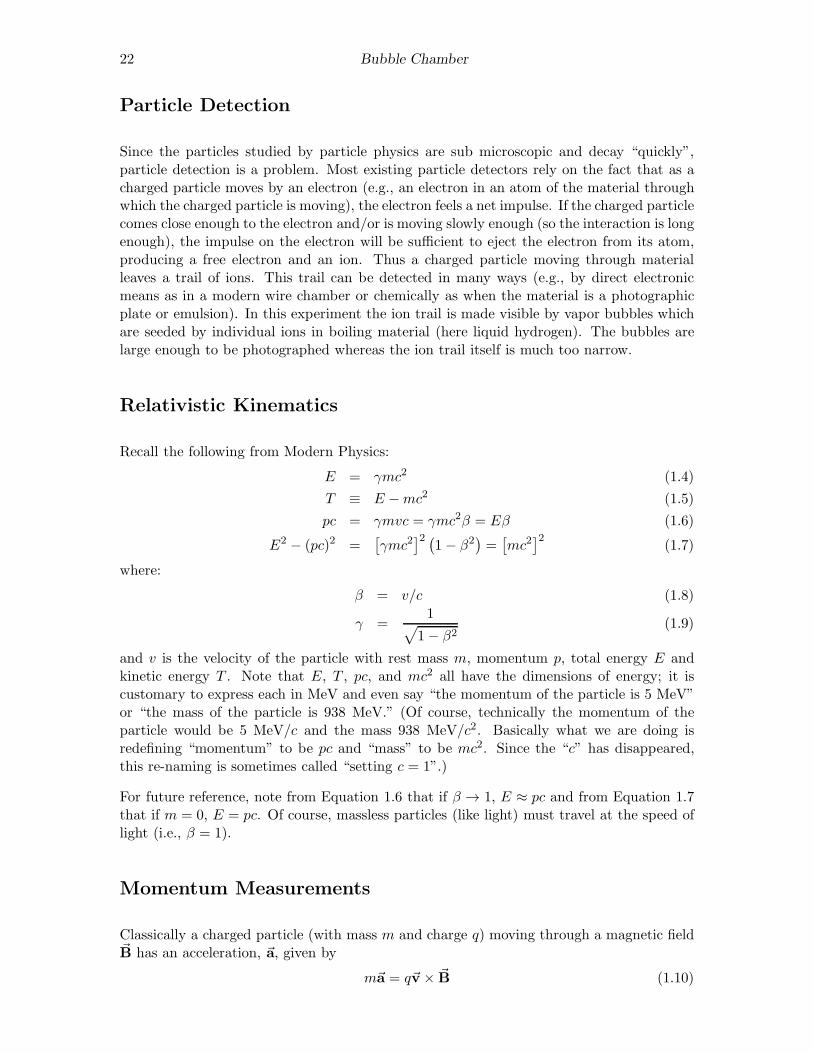
Figure 1.1: This experiment uses photographs of particle paths in a bubble chamber. Twoangles (θ ∈ [0, 180], φ ∈ [0, 360]) are required to describe the orientation of the path inthree dimensional space. The photographic (apparent) path length, L⊥, is shorter than theactual path length, L, (of course, if θ = 90, L⊥ = L). In general: L⊥ = L sin θ. The angleφ just describes the orientation of the apparent path in the photograph. We can make aneasier-to-understand model of perspective effects by just dropping φ and considering a twodimensional experiment. In this case to generate all possible orientations θ ∈ [0, 360].

For particles moving much slower than the speed of light, Newton’s mechanics is a goodapproximation: T = 1

2 mv2 = 1

2 mc2β2

L =2

2.1mc2ρ

∫ T0

0T dT =

T 20

2.1mc2ρ(1.17)

so T0 ∝ L1/2.

In this experiment muons produced by pion decay travel a distance L before coming to rest.You will measure the muon path length to determine muon T0. Since the kinetic energyof the muon comes from the rest mass of the decaying pion, the mass of the pion can becalculated from muon T0.

Perspective Effects

In real particle physics experiments, decay events are reconstructed in three dimensions.However in this experiment you will measure apparent muon path lengths from photographs.Because of perspective effects, typically the true path length (L) is longer that the appar-ent (photographic) path length (L⊥), as the particle will generally be moving towards oraway from the camera in addition to sideways. In this experiment we need to “undo” theperspective effect and determine L from the measurements of L⊥.

There are several ways this could be done. Perhaps the easiest would be to pick out thelongest L⊥, and argue that it is longest only because it is the most perpendicular, i.e.,

max (L⊥) ≈ L (1.18)

Bubble Chamber 25

.94 .83 .85 .40.49 .18 .97 .94 .28

θ

Figure 1.2: Nine randomly-oriented, fixed-length segments are placed on a plane and thecorresponding horizontal lengths L⊥ (dotted lines) are measured (results displayed belowthe segment). The resulting data set .94, .83, .85, .49, .40, .18, .97, .94, .28 of L⊥ can be an-alyzed to yield the full segment length L. (The angle θ ∈ [0, 360] describes the orientation,but it is not measured in this “experiment”: only L⊥ is measured.)

Essentially this is a bad idea because it makes use of only one collected data point (themaximum L⊥). For example, it is likely you will make at least one misidentification ormismeasurement in your 60+ measurements. If the longest L⊥ happens to be a bad point,the whole experiment is wrong. Additionally since L is the net result of interactions withrandomly placed electrons, L is not actually exactly constant. (That is, Equation 1.15 istrue only “on average”.) Paths that happen to avoid electrons are a bit longer. The L-T0relationship is based on average slowdown; it should not be applied to one special pathlength.

One way of using all the data is to note that randomly oriented, fixed-length paths willproduce a definite average L⊥ related to L. So by measuring the average L⊥ (which we willdenote with angle brackets: 〈L⊥〉), you can calculate the actual L.

It will be easier to explain this method if we drop a dimension and start by considering ran-domly oriented, fixed-length segments in two dimensions. Figure 1.2 shows3 nine randomlyoriented segments in a plane with the corresponding measured L⊥. The different measuredL⊥ are a result of differing orientations of a fixed-length segment:

L⊥ = L| sin θ| (1.19)

From a sample of N measurements of the horizontal distance L⊥ (i.e., a data set of measuredL⊥: xi for i = 1, 2, . . . , N , with corresponding orientations θi with θi ∈ [0, 2π]), theaverage L⊥ could be calculated

〈L⊥〉 =1

N

N∑

i=1

xi =L

N

N∑

i=1

| sin θi| (1.20)

The θi should be approximately evenly distributed with an average separation of ∆θ = 2π/N(because there are N angles distributed throughout [0, 2π]). Thus, using a Riemann sumapproximation for an integral:

〈L⊥〉 =L

N

N∑

i=1

| sin θi| = L

N∑

i=1

| sin θi|(

∆θ

2π

)

(1.21)

≈ L

2π

∫ 2π

0| sin θ| dθ = L

∫ 2π0 | sin θ| dθ∫ 2π0 dθ

(1.22)

3Note that if we applied Equation 1.18, we would conclude L = .97 with no estimate for the uncertaintyin this result (i.e., δL).

26 Bubble Chamber

The above integral is easily evaluated:

∫ 2π

0| sin θ| dθ = 2

∫ π

0sin θ dθ = 2

[

− cos θ]π

0= 4 (1.23)

Thus we have the desired relationship between 〈L⊥〉 and L:

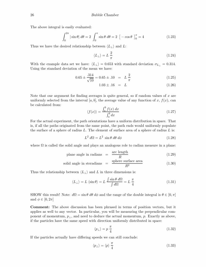
〈L⊥〉 = L2

π(1.24)

With the example data set we have: 〈L⊥〉 = 0.653 with standard deviation σL⊥= 0.314.

Using the standard deviation of the mean we have:

0.65 ± .314√10

= 0.65 ± .10 = L2

π(1.25)

1.03 ± .16 = L (1.26)

Note that our argument for finding averages is quite general, so if random values of x areuniformly selected from the interval [a, b], the average value of any function of x, f(x), canbe calculated from:

〈f(x)〉 =∫ ba f(x) dx∫ ba dx

(1.27)

For the actual experiment, the path orientations have a uniform distribution in space. Thatis, if all the paths originated from the same point, the path ends would uniformly populatethe surface of a sphere of radius L. The element of surface area of a sphere of radius L is:

L2 dΩ = L2 sin θ dθ dφ (1.28)

where Ω is called the solid angle and plays an analogous role to radian measure in a plane:

plane angle in radians =arc length

R(1.29)

solid angle in steradians =sphere surface area

R2(1.30)

Thus the relationship between 〈L⊥〉 and L in three dimensions is:

〈L⊥〉 = L 〈sin θ〉 = L

∫

sin θ dΩ∫

dΩ= L

π

4(1.31)

SHOW this result! Note: dΩ = sin θ dθ dφ and the range of the double integral is θ ∈ [0, π]and φ ∈ [0, 2π]

Comment: The above discussion has been phrased in terms of position vectors, but itapplies as well to any vector. In particular, you will be measuring the perpendicular com-ponent of momentum, p⊥, and need to deduce the actual momentum, p. Exactly as above,if the particles have the same speed with direction uniformly distributed in space:

〈p⊥〉 = pπ

4(1.32)

If the particles actually have differing speeds we can still conclude:

〈p⊥〉 = 〈p〉 π4

(1.33)

Bubble Chamber 27

0 .2 .4 .6 .8 1.0

1.0

.8

.6

.4

.2

0

L

Cum

ulat

ive

Fra

ctio

n

⊥

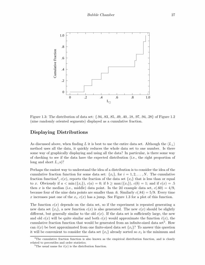
Figure 1.3: The distribution of data set: .94, .83, .85, .49, .40, .18, .97, .94, .28 of Figure 1.2(nine randomly oriented segments) displayed as a cumulative fraction.

Displaying Distributions

As discussed above, when finding L it is best to use the entire data set. Although the 〈L⊥〉method uses all the data, it quickly reduces the whole data set to one number. Is theresome way of graphically displaying and using all the data? In particular, is there some wayof checking to see if the data have the expected distribution (i.e., the right proportion oflong and short L⊥s)?

Perhaps the easiest way to understand the idea of a distribution is to consider the idea of thecumulative fraction function for some data set: xi, for i = 1, 2, . . . , N . The cumulativefraction function4, c(x), reports the fraction of the data set xi that is less than or equalto x. Obviously if a < min (xi), c(a) = 0; if b ≥ max (xi), c(b) = 1; and if c(x) = .5then x is the median (i.e., middle) data point. In the 2d example data set, c(.60) = 4/9,because four of the nine data points are smaller than .6. Similarly c(.84) = 5/9. Every timex increases past one of the xi, c(x) has a jump. See Figure 1.3 for a plot of this function.

The function c(x) depends on the data set, so if the experiment is repeated generating anew data set xi, a new function c(x) is also generated. The new c(x) should be slightlydifferent, but generally similar to the old c(x). If the data set is sufficiently large, the newand old c(x) will be quite similar and both c(x) would approximate the function c(x), thecumulative fraction function that would be generated from an infinite-sized data set5. Howcan c(x) be best approximated from one finite-sized data set xi? To answer this questionit will be convenient to consider the data set xi already sorted so x1 is the minimum and

4The cumulative fraction function is also known as the empirical distribution function, and is closelyrelated to percentiles and order statistics.

5The usual name for c(x) is the distribution function.

28 Bubble Chamber

0 .2 .4 .6 .8 1.0

1.0

.8

.6

.4

.2

0

L

Cum

ulat

ive

Fra

ctio

n

⊥

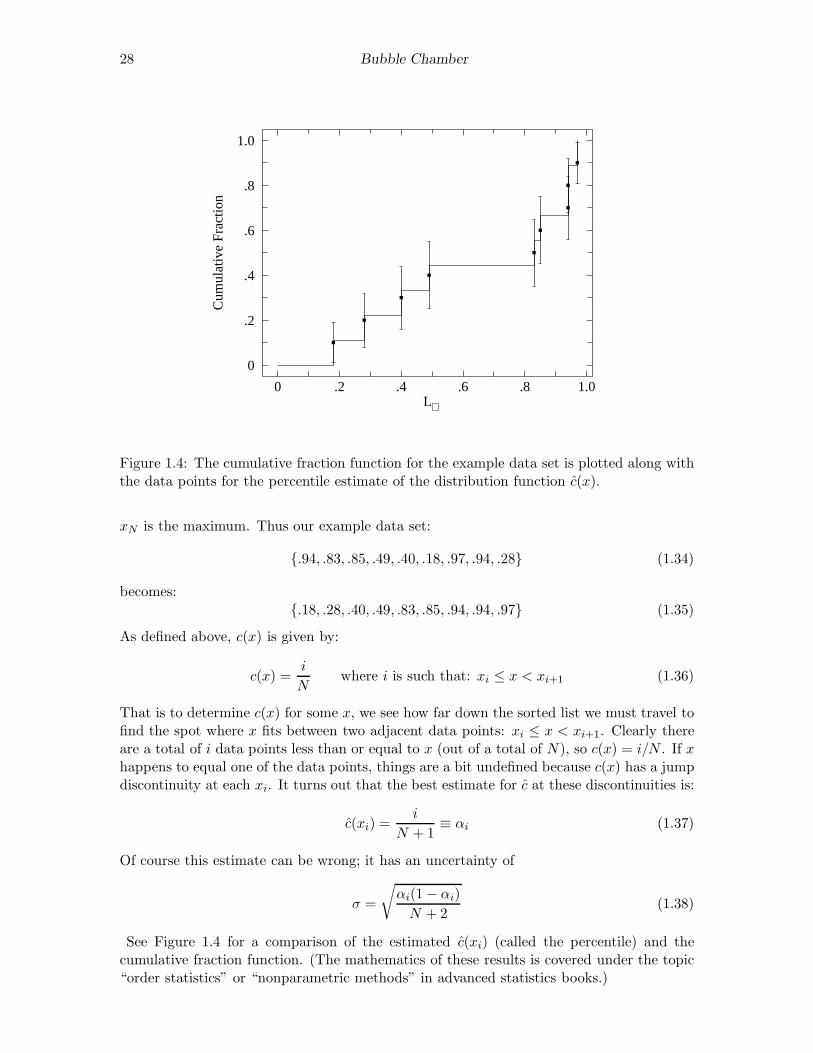
Figure 1.4: The cumulative fraction function for the example data set is plotted along withthe data points for the percentile estimate of the distribution function c(x).

xN is the maximum. Thus our example data set:

.94, .83, .85, .49, .40, .18, .97, .94, .28 (1.34)

becomes:

.18, .28, .40, .49, .83, .85, .94, .94, .97 (1.35)

As defined above, c(x) is given by:

c(x) =i

Nwhere i is such that: xi ≤ x < xi+1 (1.36)

That is to determine c(x) for some x, we see how far down the sorted list we must travel tofind the spot where x fits between two adjacent data points: xi ≤ x < xi+1. Clearly thereare a total of i data points less than or equal to x (out of a total of N), so c(x) = i/N . If xhappens to equal one of the data points, things are a bit undefined because c(x) has a jumpdiscontinuity at each xi. It turns out that the best estimate for c at these discontinuities is:

c(xi) =i

N + 1≡ αi (1.37)

Of course this estimate can be wrong; it has an uncertainty of

σ =

√

αi(1− αi)

N + 2(1.38)

See Figure 1.4 for a comparison of the estimated c(xi) (called the percentile) and thecumulative fraction function. (The mathematics of these results is covered under the topic“order statistics” or “nonparametric methods” in advanced statistics books.)

Bubble Chamber 29

θ

Figure 1.5: A particular line segment is displayed along with the measured L⊥ (dotted line).What fraction of randomly oriented segments would have a L⊥ smaller than this particularsegment? The darkly shaded part of the circle shows possible locations for these small L⊥segments. The fraction of such small L⊥ segments should be the same as the dark fractionof the circle: 4θ/2π.

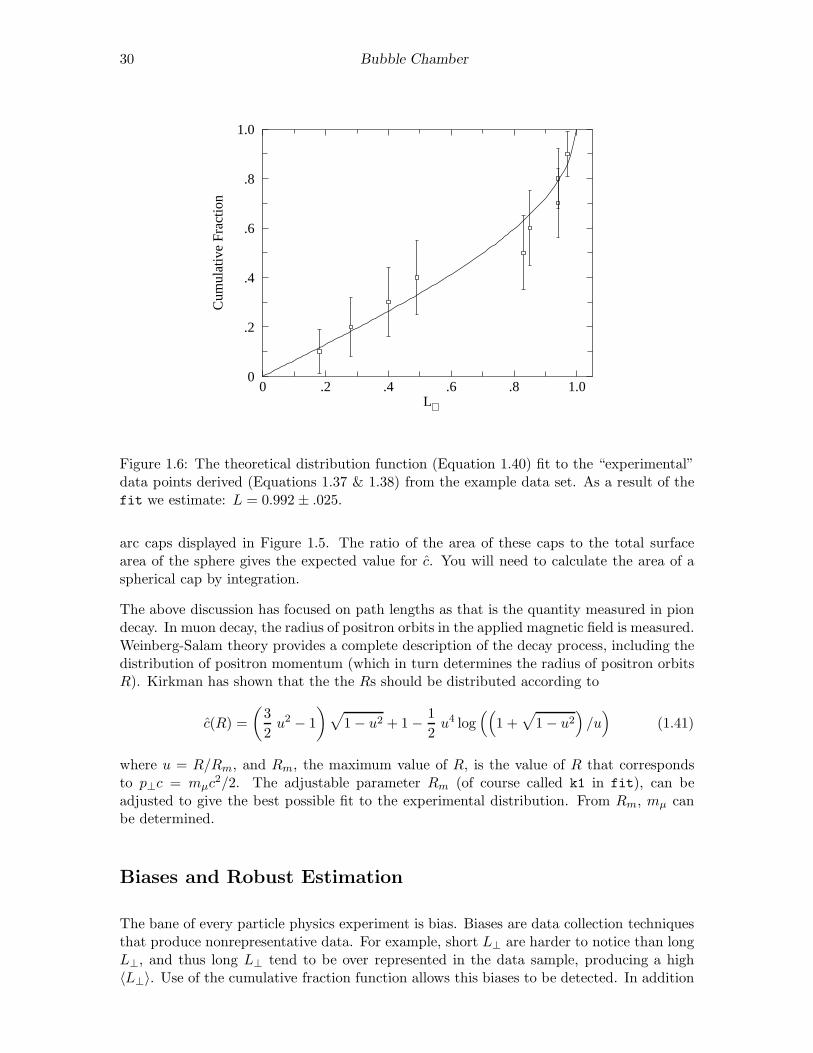
Your experimental estimate of c should be compared to the theoretically expected c. Theexample data set was generated from randomly oriented line segments in a plane. As shownin Figure 1.5, it is expected that the fraction of a data set less than some particular valueof L⊥ is:

c(L⊥) =4θ

2πwhere: θ = arcsin(L⊥/L) (1.39)

=2

πarcsin(L⊥/L) (1.40)

Our formula for c involves the unknown parameter L; we adjust this parameter to achievethe best possible fit to our experimental estimate for c. Using the program fit:

tkirkman@bardeen 7% fit

* set f(x)=2*asin(x/k1)/pi k1=1.

* read file cf.L.dat

* fit

Enter list of Ks to vary, e.g. K1-K3,K5 k1

FIT finished with change in chi-square= 5.4810762E-02

3 iterations used

REDUCED chi-squared= 0.2289333 chi-squared= 1.831467

K1= 0.9922597

Using the covariance matrix to determine errors6, we conclude k1 = 0.992 ± .025. Thisreported random error is about 1

6 that obtained above using 〈L⊥〉.

SHOW: Derive yourself the theoretical function c(L⊥) for line segments in space. Hint:Begin by noting that if the segments shared a common origin, the segment ends woulduniformly populate the surface of a sphere of radius L. Segments with measured L⊥ lessthan some particular value would lie on a spherical cap, the three dimensional version of

6Reference 2, Press et al., says usually error estimates should be based on the square root of the diagonalelements of the covariance matrix

30 Bubble Chamber

0 .2 .4 .6 .8 1.0

1.0

.8

.6

.4

.2

0

L

Cum

ulat

ive

Fra

ctio

n

⊥

Figure 1.6: The theoretical distribution function (Equation 1.40) fit to the “experimental”data points derived (Equations 1.37 & 1.38) from the example data set. As a result of thefit we estimate: L = 0.992 ± .025.

arc caps displayed in Figure 1.5. The ratio of the area of these caps to the total surfacearea of the sphere gives the expected value for c. You will need to calculate the area of aspherical cap by integration.

The above discussion has focused on path lengths as that is the quantity measured in piondecay. In muon decay, the radius of positron orbits in the applied magnetic field is measured.Weinberg-Salam theory provides a complete description of the decay process, including thedistribution of positron momentum (which in turn determines the radius of positron orbitsR). Kirkman has shown that the the Rs should be distributed according to

c(R) =

(

3

2u2 − 1

)

√

1− u2 + 1− 1

2u4 log

((

1 +√

1− u2)

/u)

(1.41)

where u = R/Rm, and Rm, the maximum value of R, is the value of R that correspondsto p⊥c = mµc

2/2. The adjustable parameter Rm (of course called k1 in fit), can beadjusted to give the best possible fit to the experimental distribution. From Rm, mµ canbe determined.

Biases and Robust Estimation

The bane of every particle physics experiment is bias. Biases are data collection techniquesthat produce nonrepresentative data. For example, short L⊥ are harder to notice than longL⊥, and thus long L⊥ tend to be over represented in the data sample, producing a high〈L⊥〉. Use of the cumulative fraction function allows this biases to be detected. In addition

Bubble Chamber 31

to biases, the cumulative fraction function allows you to detect likely mistakes: for example,particle path lengths that are extraordinary given the entire data set.

The detection of a likely mistake suggests corrective actions like removing the “bad” point.You should almost never do this! (You will find a chapter in Taylor on this “awkward” and“controversial” problem.) A better option is to use analysis methods that are “robust”, i.e.,that are insensitive to individual “bad” points.7 Imagine we modify our example data setby adding a “bad” point: L⊥ = 2:

.18, .28, .40, .49, .83, .85, .94, .94, .97, 2.00 (1.42)

Adding this outlying8 data point totally messes up the max(L⊥) method (the least robustmethod). Since it increases both the mean and the standard deviation, the estimated Lbased on the 〈L⊥〉 method shifts from 1.03 ± .16 to 1.24 ± .26.

Changing the number of data points requires recalculating the estimated distribution func-tion for every point (because the value of c depends on the set size N). If we carry throughthe total analysis with our enlarged data set we find the fit L shifts from 0.992 ± .025 to1.05 ± .05. We can conclude that the cumulative fraction method is less sensitive to baddata than the average method.9

Unconscious (uncontrolled) biases produce tainted data which can be rescued in part byrobust estimation. Once bias is recognized the experiment can be rearranged to adjustfor its effects. This requires that the bias be exactly reproducible. For example, shortapparent muon paths (paths mostly towards or away from the camera) are inconspicuousand hence more likely to be missed on some occasions. One solution is formalize this biasand intentionally ignore all photographic paths shorter than say .3 cm long (about 5% ofthe data). This cut (formalized noncollection of data), can be included in the theoreticaldistribution function so it will not affect parameter estimation.

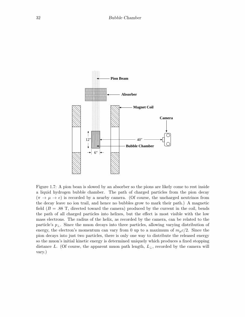
Experimental Arrangement

Our bubble chamber photographs were taken using the 385 MeV proton accelerator atNevis Lab which is a part of Columbia University. A pion beam was produced by collidingaccelerated protons with a copper target. The pion beam was directed through an absorberto slow the pions so that a sizable fraction of the pions would come to rest in the adjacentbubble chamber. See Figure 1.7. The path of charged particles from the pion decay (π →µ → e) as recorded by a nearby camera, encodes the information needed to calculate mπ

7Removing a data point is a lie. A more subtle sort of lie comes from the existence of choice of methods.Clearly, you can analyze the data several different ways, and then present only the method that producesthe answer you want. Darrell Huff’s book How to Lie with Statistics (Norton, 1954) can help you if that isyour goal. I probably don’t need to remind you that schools with “Saint” in their name do not recommendthis course of action. Choice and ethics are interlocking concepts.

8While not exactly relevant, this data point is 2.34×σ above the mean and hence an outlier by Chauvenet’scriterion (see Reference 4, Taylor). It is also an outlier by Tukey’s criterion (see Reference 3, Hogg & Tanis).

9Do note that both results remain consistent with the intended value of 1.00. Also note that the mediancould have provided a more robust alternative to the average. However, that would have required a discussionof the uncertainty in the median, which is beyond the intended aims of this lab. In this lab—and in mostany experiment—there are many possible ways to analyze the data. Choice of method often involves artand ethics.

32 Bubble Chamber

99999999999999999999999999999999999999999999999999999999999999999999999999999999999999999996"

12"

99999999999999999999999999999999999999999999999999999999999999999999999999999999999999999999999999

9999999999999999999999999999999999999999999999999999999999999999999999999999999999999999999

99999999999999999999999999999999999999999999999999999999999999999999999999999999999999999999999999

40"

000000000000000000000000000000000000000000000000000000000000000000000000000000000000000000000000000000000000000000000000000000

Pion Beam

Absorber

Magnet Coil

Camera

Bubble Chamber

Figure 1.7: A pion bean is slowed by an absorber so the pions are likely come to rest insidea liquid hydrogen bubble chamber. The path of charged particles from the pion decay(π → µ → e) is recorded by a nearby camera. (Of course, the uncharged neutrinos fromthe decay leave no ion trail, and hence no bubbles grow to mark their path.) A magneticfield (B = .88 T, directed toward the camera) produced by the current in the coil, bendsthe path of all charged particles into helixes, but the effect is most visible with the lowmass electrons. The radius of the helix, as recorded by the camera, can be related to theparticle’s p⊥. Since the muon decays into three particles, allowing varying distribution ofenergy, the electron’s momentum can vary from 0 up to a maximum of mµc/2. Since thepion decays into just two particles, there is only one way to distribute the released energyso the muon’s initial kinetic energy is determined uniquely which produces a fixed stoppingdistance L. (Of course, the apparent muon path length, L⊥, recorded by the camera willvary.)

Bubble Chamber 33

incomingpion

stationarypion decays

muonpath

stationarymuon decays

electronpath

µ−

ν

ν

e−π−

ν

key

magnetic fieldpoints out of pageB

→

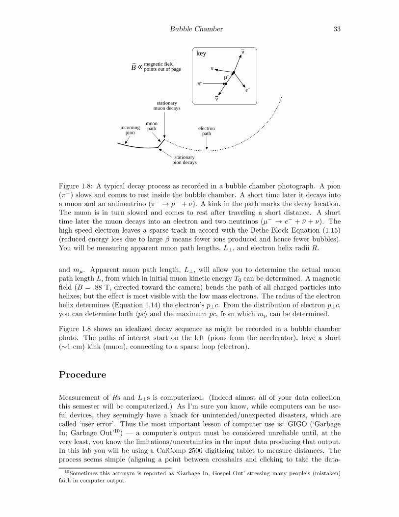
Figure 1.8: A typical decay process as recorded in a bubble chamber photograph. A pion(π−) slows and comes to rest inside the bubble chamber. A short time later it decays intoa muon and an antineutrino (π− → µ− + ν). A kink in the path marks the decay location.The muon is in turn slowed and comes to rest after traveling a short distance. A shorttime later the muon decays into an electron and two neutrinos (µ− → e− + ν + ν). Thehigh speed electron leaves a sparse track in accord with the Bethe-Block Equation (1.15)(reduced energy loss due to large β means fewer ions produced and hence fewer bubbles).You will be measuring apparent muon path lengths, L⊥, and electron helix radii R.

and mµ. Apparent muon path length, L⊥, will allow you to determine the actual muonpath length L, from which in initial muon kinetic energy T0 can be determined. A magneticfield (B = .88 T, directed toward the camera) bends the path of all charged particles intohelixes; but the effect is most visible with the low mass electrons. The radius of the electronhelix determines (Equation 1.14) the electron’s p⊥c. From the distribution of electron p⊥c,you can determine both 〈pc〉 and the maximum pc, from which mµ can be determined.

Figure 1.8 shows an idealized decay sequence as might be recorded in a bubble chamberphoto. The paths of interest start on the left (pions from the accelerator), have a short(∼1 cm) kink (muon), connecting to a sparse loop (electron).

Procedure

Measurement of Rs and L⊥s is computerized. (Indeed almost all of your data collectionthis semester will be computerized.) As I’m sure you know, while computers can be use-ful devices, they seemingly have a knack for unintended/unexpected disasters, which arecalled ‘user error’. Thus the most important lesson of computer use is: GIGO (‘GarbageIn; Garbage Out’10) — a computer’s output must be considered unreliable until, at thevery least, you know the limitations/uncertainties in the input data producing that output.In this lab you will be using a CalComp 2500 digitizing tablet to measure distances. Theprocess seems simple (aligning a point between crosshairs and clicking to take the data-

10Sometimes this acronym is reported as ‘Garbage In, Gospel Out’ stressing many people’s (mistaken)faith in computer output.

34 Bubble Chamber

point) but involves problem of definition errors (including systematic biases, see page 13) inaddition to more familiar device limitations (random and calibration errors). To have somejustified confidence in this process, you must measure a known and see what the computerreports (‘trust, but verify’). I have provided you with a simulated bubble chamber photoin which all the path lengths are 1 cm and all the curvatures are 20 cm. (If you don’t trustthis fiducial—and you might not since it depends on the dimensional stability of printersand paper—you can measure the ‘tracks’ with an instrument you do trust.) Begin by log-ging into your linux account using the Visual 603 terminal with attached CalComp 2500digitizer, and running the program bubbleCAL:

tkirkman@linphys8 1% bubbleCAL

The following directions are displayed:

The general procedure will be to place the cursor crosshair at

the needed place and press a cursor button to digitize. Press

cursor button "0" when obtaining muon path lengths (digitize

beginning and end of track); press cursor button "1" when obtaining

electron radii of curvature (digitize three points on curve, from

which the computer can figure R); press cursor button "2" to cancel

an in-progress data point or clear error; press cursor button "3" to

remove the last data point of the presently selected type. Additional

data points may be removed by number when done. Digitizer will beep

between data points. Hit ^D (control D) on keyboard when done.

Files containing your data (unsorted) will be created: Lcal.DAT & Rcal.DAT.

THIS PROGRAM IS FOR CALIBRATION/TESTING NOT DATA COLLECTION

With the simulated bubble chamber photo taped in place on the digitizer, check some longdistances (> 10 cm) on the scales. Then measure 16 path lengths and 16 curvatures. Recordthe data reported by the program (means, standard deviations, 95% confidence intervals,etc.). Does the probable range for each mean include the known value? (If not discuss theproblem with Dr. Kirkman.) Note that if you took more data points, the probable range forthe mean would become increasingly small and eventually you would detect a systematicerror limiting the ultimate accuracy of the device.

The program bubble works very much like bubbleCAL, except in the end it will producefiles containing the cumulative fraction of L⊥ (cf.L.dat) and R (cf.R.dat). Please do notdeface the bubble chamber photos! Lightly tape each bubble chamber photograph to thedigitizer to keep the photo from moving as you collect data. Collect ∼ 64 L⊥s and ∼ 64 Rs.(This will require scanning about 20 bubble chamber photos.) The program will make fourfiles: cf.R.dat contains the usual three columns: R, the percentile estimate c(R) calculatedfrom your data, and the error in the estimate, cf.L.dat similarly contains the sorted L⊥,estimated c(L⊥) and error, L.DAT and R.DAT contain the (unsorted) raw data.

Use the web11 or gnumeric (Linux spreadsheet) to calculate 〈L⊥〉 and 〈R〉 and their standarddeviations. Note that the raw data files (L.DAT and R.DAT) can be used to transfer the datato these applications.

11http://www.physics.csbsju.edu/stats/cstats paste form.html

Bubble Chamber 35

Use fit (see page 171) to fit each dataset (cf.R.dat & cf.L.dat) to the appropriatetheoretical distribution function. Produce a hardcopy of your fit results to include in yournotebook. Use plot (see page 177) to produce a hardcopy plot of your data with fittedcurve to include in your notebook. (Copy and paste is the easiest way to accurately transferK1 between fit and plot.)

The formula for c(R) (Eq. 1.41) is a bit tricky to type in, so I’ve provided you with ashortcut: c(R) will be automatically entered as f(x) into fit or plot if you type:

* @/usr/local/physics/help/cr.fun

In this f(x), K1 holds the parameter Rm, x is a measured R, and f(x) is the expected valuec(R).

Calculation of mµ

Since energy is conserved, the rest energy of the muon must end up in its decay products:

Eµ = mµc2 = Ee + Eν + Eν (1.43)

where Eµ, Ee, Eν , Eν are respectively the total energy of the muon, electron, neutrino, andantineutrino.

You should expect that the rest energy of the muon would, on average, be evenly dividedbetween the three particles. Thus

〈Ee〉 ≈ 〈Eν〉 ≈ 〈Eν〉 ≈1

3mµc

2 (1.44)

In fact, the Weinberg-Salam theory of weak decays predicts

〈Ee〉 = .35mµc2 (1.45)

Since electrons with that much energy have β = .9996, to a good approximation Ee = pec.Thus

.35mµc2 = 〈Ee〉 = 〈pec〉 =

4

π〈pe⊥c〉 (1.46)

so you will find mµc2 from 〈pe⊥c〉 (which, in turn, may be found from 〈R〉).

Additionally, you will calculate mµc2 from your fit value of Rm (using your data and the

theoretical expression for c(R), Equation 1.41). From the above discussion you alreadyknow

3BRm = p⊥c = mµc2/2 (1.47)

allowing you to determine mµc2 from B and Rm.

Recall: Standard deviation of the mean is used for errors in averages (see Taylor). Thesquare root of the diagonal elements of the covariance matrix determine the errors in fit

parameters (See Press, et al.).

36 Bubble Chamber

Calculation of mπ

The pion mass can be determined from the muon path length L: From L you can find theinitial kinetic energy of the muon (T0); adding the rest energy of the muon (use a highaccuracy book-value for mµc

2) gives you the total muon energy, Eµ.

Eµ = T0 +mµc2 (1.48)

From momentum conservation and the fact the neutrinos have nearly zero rest mass andhence travel at the speed of light, you can show

Eν = pνc = pµc =[

E2µ − (mµc

2)2]1/2

(1.49)

Finally, energy conservation of the decaying pion requires

mπc2 = Eµ + Eν = Eµ +

[

E2µ − (mµc

2)2]1/2

(1.50)

from which mπc2 can be calculated.

We have discussed two ways of determining L (using Equation 1.31 with a measured valuefor 〈L⊥〉 and by fitting the theoretical c(L⊥) curve to your experimental data), so you willproduce two values for mπ.

Note: The error in the book value of mµ used to calculate mπ should be small enough toignore, so the error in mπc

2 (δmπc2) is due to the uncertainty in L (given by fit) or the

uncertainty in 〈L⊥〉 (given by the standard deviation of the mean). To calculate δmπc2,

find∂mπc

2

∂Eµand δEµ = δT0 and apply Eq. E.9 (or E.12) in the form:

δmπc2 =

∂mπc2

∂EµδEµ (1.51)

Some Words About Errors

We noted above that different analysis methods yield different statistical error estimates.And robust methods that produce smaller uncertainties are preferred. But no amount ofstatistical gamesmanship can erase a systematic error in the original measurements so thereis little point in reducing statistical errors once systematic errors dominate. Said differently:the aim is to understand the systematic errors and then reduce the statistical errors untilthey become irrelevant.

In this experiment one finds potential systematic errors in constants given without error(B = .88 T, ρ = .07 g/cm3, the “2.1” in the Bethe-Block Equation 1.15) and theoreticalsimplifications (the bubble chamber’s 6” thickness means paths closer to the camera areenlarged in photographs compared to those further from the camera, ‘straggling’ where somemuons would have stopping distances a bit more or less than that calculated from the Bethe-Block Equation, varying magnetic field within the bubble chamber, expansion/contractionof the photographs due varying to humidity).

Bubble Chamber 37

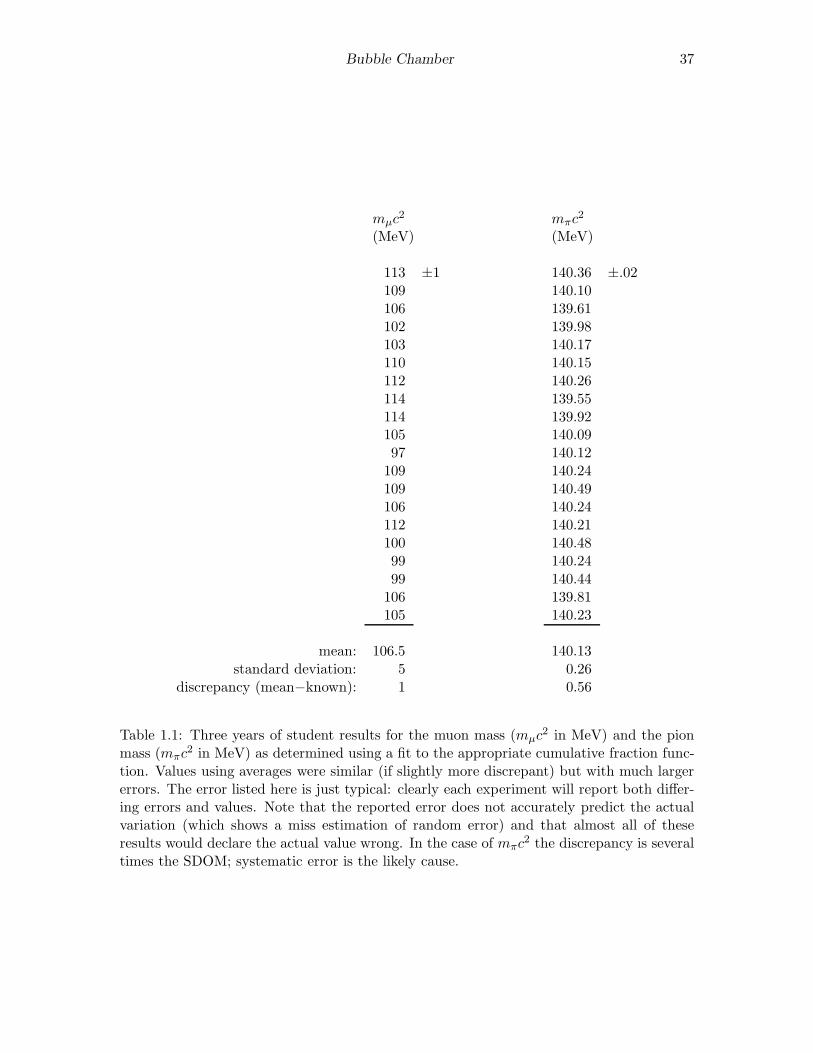
mµc2 mπc

2

(MeV) (MeV)

113 ±1 140.36 ±.02109 140.10106 139.61102 139.98103 140.17110 140.15112 140.26114 139.55114 139.92105 140.0997 140.12109 140.24109 140.49106 140.24112 140.21100 140.4899 140.2499 140.44106 139.81105 140.23

mean: 106.5 140.13standard deviation: 5 0.26

discrepancy (mean−known): 1 0.56

Table 1.1: Three years of student results for the muon mass (mµc2 in MeV) and the pion

mass (mπc2 in MeV) as determined using a fit to the appropriate cumulative fraction func-

tion. Values using averages were similar (if slightly more discrepant) but with much largererrors. The error listed here is just typical: clearly each experiment will report both differ-ing errors and values. Note that the reported error does not accurately predict the actualvariation (which shows a miss estimation of random error) and that almost all of theseresults would declare the actual value wrong. In the case of mπc

2 the discrepancy is severaltimes the SDOM; systematic error is the likely cause.

38 Bubble Chamber

The error in L determined from the fit to the theoretical cumulative fraction function is oftenobviously too-small12. The covariance matrix typically suggests an L error of about .001 cm.Whereas bubbleCAL typically suggests systematic errors in L measurements greater than.01 cm. Further the likely error in the ρ and 2.1 that occur together with L in Eq. 1.17,would suggest L accuracy below 5% is irrelevant.

It is helpful to review multiple results collected over several years given in Table 1.1. Themean discrepancy is not too worrisome: a few percent change in the given constants woulderase that difference. Of greater concern is large mismatch between the calculated statisticalerror and the standard deviation upon repeated measurement with identical equipment(but different data collectors). I’m sure part of this variation is due to ‘personal placementdecision’ detected by bubbleCAL, but additionally varying ability to notice short L⊥ willcreate varying results. (Most student cumulative fraction plots show a deficit of short L⊥.)In any case we see here an example of calculated statistical errors reduced way below otheruncontrolled uncertainties.

Given this table of experiment repeats, would it be fair to report the standard deviation ofthe mean as the uncertainty in, say mπc

2? Numerically you can see that the result wouldbe disastrous (as the SDOM is about 1

10 the discrepancy). Since we are attributing thedeviation to different observers (since the equipment and photos are the same) and we haveno right to suggest that the average observer is the perfect observer (indeed one might saythe perfect observer is exceptional), the answer must be “No”. In short you can only usethe SDOM as the error if you are convinced the deviation is caused by a balanced (exactlyas much high as low) process. (And that implies you have a good idea of what is causingthe deviations.)

In our experiment, the actual experimental error is available to us (since mµ and mπ havesince been measured to high accuracy), but how could the original investigators estimatethese errors? A short answer to this question is calibration: “placing” known pathlengthsand radii into the bubble chamber, and comparing the known values to the measured results.Indeed, experiments exactly like this lab are used to calibrate the detection systems inmodern experiments.

Histograms

The cumulative fraction function described above is generally used when fewer then a thou-sand data points are available. Histograms are a more familiar way of displaying distribu-tions. Histograms are made by dividing the range of the data set xi into several (usuallyequal-sized) sub intervals call bins. The data are sorted into these bins, and the numberof data points in each bin is recorded as the y value for the average x value of the bin.(According to Poisson statistics, the uncertainty in y would be the square root of y.) Theresulting plot is closely related to dc/dx (also known as the probability density function).Histograms are valued because they immediately show which bins are highly populated,i.e., what values of x occur frequently.

12The reason too-small errors are found when fitting to cumulative fraction functions may be found inReference 2, Press, et al.

Bubble Chamber 39

Report Checklist

1. Write an introductory paragraph describing the basic physics behind this experiment.For example, why did different decays of pions result in different L⊥? Why diddifferent decays of muons result in different R? What are the relationships betweenL⊥, R and more usual variables of motion? (This manual has many pages on thesetopics; your job is condense this into a few sentences and no equations.)

2. Book values for muon (µ±) and charged pion (π±) mass. Find (and cite) a sourcethat reports at least five significant digits.

3. Derivations:

(a) Equation 1.14

(b) Equation 1.31

(c) Area of a spherical cap

(d) Use above to derive c(L⊥)

4. Read: http://www.physics.csbsju.edu/stats/display.distribution.htmlLet’s call the last two digits of your CSB/SJU ID number: XY.

(a) Go to the web site: http://www.physics.csbsju.edu/370/data/ and selectthe file: 4 X.dat. This file contains 4 random data points. By hand draw inyour notebook the cumulative fraction step-curve for this dataset along with thepercentile values with errors. The result should be similar to Figure 1.4. Showyour work!

(b) From the same web site, select the file: 1000 Y.dat (or 1000 Yw.dat with thesame data in multiple columns). Select reasonable bin values and by hand drawthe histogram for this dataset including error bars. Show your work! Copy &paste the 1000 data points into the web13 site and produce a hardcopy percentileplot. Comment on the relationship between features in your histogram andfeatures in the percentile plot.

(Note: I’m requesting individual work—rather than partnered work—to check thateveryone understands these plots. Do feel free to help your partner succeed, but don’tjust do the work for him/her.)

5. Results and conclusions from use of the program bubbleCAL: Was systematic errordetected? If so, how much. If not, how large could the systematic have been and stillgo undetected? (This is called an upper limit on the error.) Compare your systematicerror (detected or upper limit) in L and R to the fit supplied estimates of randomerror in L and Rm. Which is more significant: random or systematic error?

6. Two values (with errors) for mµ: one based on 〈R〉 (see Eq. 1.46) and the other on afit to Equation 1.41. Hardcopies of the fit results and a plot of the best-fit curvewith your data points. (The plot is analogous to Figure 1.6.)

7. Two values (with errors) for mπ: one based on L found from 〈L⊥〉 using Eq. 1.31 andthe other based on L found from the fit to the equation for c(L⊥) you derived in3(d) above. Hardcopies of the fit results and a plot of the best-fit curve with yourdata points.

13http://www.physics.csbsju.edu/stats/cstats paste form.html

40 Bubble Chamber

8. A comparison of the mass values you reported above (6 & 7) and the “known” valuescited above in 2. (Make a nice table.)

9. Typically in this lab, the error estimates based on fits that are much smaller than theerrors based on averages. Are these error estimates accurate? (If your masses (witherrors) are inconsistent with book values, it is quite likely that something is wrongwith your error estimates.) Explain how your error estimates could be improved. (Forexample, sometimes error estimates can be improved (and reduced) by simply takingmore data. In other situations, improved errors come from proper consideration ofsystematic errors and result in larger estimates of error.) A few words about statisticaland systematic errors are probably required; you might consult Chapter 0 if nothingoccurs to you.

References

1. Lederman, Leon & Teresi, Dick The God Particle (1993)— In this general-audiencebook Nobel Laureate Lederman describes his work as an experimental particle physi-cist. Of particular interest: his work with pions in a cloud chamber using the Nevisaccelerator (pp. 219–224); building cloud and bubble chambers (pp. 244–247); parityviolation detected in the π → µ→ e decay sequence (pp. 256–273).

2. Press, Teukolsky, Vetterling & Flannery Numerical Recipes (1992)— Title says itall. Cumulative fraction is discussed in the section on the Kolmogorov-Smirnov Test;covariance matrix in chapter on modeling data.

3. Hogg & Tanis Probability and Statistical Inference (1993)— Order statistics are dis-cussed in Chapter 10.

4. Taylor, J.R. An Introduction to Error Analysis (1997)— derivative rule error propa-gation, standard deviation of the mean, histograms, random and systematic errors

5. I know of no book that derives Equation 1.41. A starting point is the Kurie Plot forweak decays, for example, from Halzan & Martin Quarks and Leptons (1984) p. 263:

dΓ

dE=

G2

12π3m2 E2

(

3− 4E

m

)

(1.52)

6. Enge, H.A. Introduction to Nuclear Physics (1966)— Chapter 7 has a nice discussionon stopping power, range, the Bethe-Block equation and particle detectors includingbubble chambers.

7. Coughlan, G. D. & Dodd, J. E. The Ideas of Particle Physics: An Introduction forScientists (2003)— An excellent introduction to particle physics at undergraduatephysics major level.

8. This lab is based on “The Pi-Mu-e Experiment” 33-3908 (1966) by Ealing Corporation.

2: Photometry

The mathematical thermology created by Fourier may tempt us to hope that. . . wemay in time ascertain the mean temperature of the heavenly bodies: but I regardthis order of facts as forever excluded from our recognition.

Auguste Comte Cours de la Philosophie Positive1 (1835)

. . . within a comparatively few years, a new branch of astronomy has arisenwhich studies the sun, moon, and stars for what they are in themselves and inrelation to ourselves.

Samuel Pierpont Langley The New Astronomy (1888)

Purpose

In 1835 the French philosopher Auguste Comte noted that since we know stars only bytheir light (and cannot take bits of stars into the laboratory), our knowledge of stars wouldbe forever limited essentially to location. Fifty years later astrophysics—the study of thephysics of stars—was beginning, and the first measurements of the Sun’s temperature andcomposition were being made. Evidently, careful measurement of starlight (photometry)allows the intrinsic properties of stars to be determined. In this lab you will use broadbandphotometry to measure the temperature of stars.

Introduction

We begin our study of stars with blackbody radiation, which you studied in Modern Physicsand you will yourself measure in the Thermionic Emission lab (p. 115). The light producedby a hot object is akin to audio noise: in both cases a random process produces a simul-taneous superposition of a wide distribution of wavelengths. In his Opticks, Newton notedcertain systematic dependencies in the light emitted by incandescent objects and suggestedsomething fundamental was behind the process2. Apparently the light produced by an in-candescent object is fundamentally related to its temperature not its material composition.In 1879 Joseph Stefan proposed that every object emits light energy at the rate (power in

1http://socserv2.mcmaster.ca/~econ/ugcm/3ll3/comte/ provides this as an etext translated andedited by Harriet Martineau.

2Query 8: Do not all fix’d Bodies, when heated beyond a certain degree, emit Light and shine. . .Query 11:. . . And are not the Sun and fix’d Stars great Earths vehemently hot. . .

41

42 Photometry

watts):P = ǫTσT

4A (2.1)

where σ is the Stefan-Boltzmann3 constant, T is the temperature of the body, A is thesurface area of the body, and ǫT is the total emissivity.

Experimentally it was found that the wavelength distribution of the light from hot objectswas broadly similar to the Maxwell-Boltzmann speed distribution: a bell-shaped curve inwhich the location of the peak depended on temperature. In 1893 Wilhelm Wien4 concludedthat the wavelength of this peak must be inversely proportional to temperature. Experimentconfirmed that the wavelength of this peak was given by:

λmax =2898 µm ·K

T(2.2)

Together the Stefan-Boltzmann and Wien displacement laws—both the results of classicalphysics—explain much of what is commonly observed in hot objects. At room tempera-ture objects do not appear to be a source of light: they appear dark (unless externallyilluminated). This is a result both of the small rate of emission given by Stefan-Boltzmannand (from Wien) for T = 300 K, we find λmax ∼ 10 µm, that is the wavelengths typicallyemitted are well outside the range of light that can be detected by the eye5. On the otherhand for an object like the Sun: T ≈ 6000 K, so λmax ∼ 0.5 µm — right in the middle ofof the visible range.

Our ‘spherical cow’ model6 of a star is an incandescent ball (radius R) of gas shining as ablackbody. Thus the total power output of a star (called the luminosity7) is

L = σT 4 4πR2 (2.3)

The equation for the exact distribution of photon wavelengths produced by a blackbodywas actively researched with erroneous equations produced by Wien and Rayleigh & Jeans.In 1900 Max Planck8 published his derivation of the wavelength distribution of light froma blackbody. However before we can discuss his result we must explain what precisely ismeant by ‘wavelength distribution’.

In Physics 211 you learned about the speed distribution9 of the molecules in a gas: abell-shaped curve that shows that slow molecules are rare and supersonic molecules are

3In 1879 Jozef Stefan (1835–93) proposed the law based on experimental measurements; five years laterLudwig Boltzmann (1844–1906) derived the result from fundamental thermodynamics. Today the result isknown as the Stefan-Boltzmann Law.

4Wilhelm Wien (1864–1928) German physicist, 1911 Nobel Prize in Physics5The human eye can detect light with a wavelength in the range 0.4 µm (violet) to 0.7 µm (red).6This model of a star works best with stars similar in temperature to the Sun, but every star’s light is

considerably modified by absorption as it travels through the star’s atmosphere. In hot stars, UV wavelengthsthat can photoionize hydrogen (H(n = 2)+γ → H++e−) are highly attenuated producing the Balmer jump.The spectra of cool stars shows broad absorption bands due to molecules.http://www.jb.man.ac.uk/distance/life/sample/java/spectype/specplot.htm is an applet allowing acomparison of blackbody light to actual star light.

7The MKS unit for luminosity is watt, but the numbers are so large that it is usually expressed as amultiple (or fraction) of the Sun’s luminosity (a.k.a., solar luminosity) L⊙ = 3.846 × 1026 W.

8Max Planck (1858–1947) German physicist, 1918 Nobel Prize in Physics9Derived by James Clerk Maxwell (1831–1879); Ludwig Boltzmann (1844–1906) provided a firm founda-

tion for the result using statistical mechanics. Today the result is generally known as the Maxwell-Boltzmanndistribution.

Photometry 43

0 .5 1.0 1.5 2.0

10.E+07

8.E+07

6.E+07

4.E+07

2.E+07

0

Blackbody Thermal Radiation

wavelength ( m)

F (

W/m

m

)

6000 K

4000 K

µ

µλ

2

Figure 2.1: The distribution of the light emitted by a blackbody plotted as a function ofwavelength. Hotter objects emit much more light than cool ones, particularly at the shorterwavelengths.

rare, whereas a molecular kinetic energy near 32kT is common. ‘Speed probability’ is a

problematic concept. For example the probability that a molecule has a speed of exactlyπ m/s (or any other real number) must be essentially zero10 (as an infinite number of digitsmust match, but there are only a finite [but huge] number of molecules). Probability densityprovides a meaningful context to talk about speed distribution: determine the fraction ofmolecules (‘hits’) that have speed in an interval (bin) (v−∆v/2, v+∆v/2) for various speedsv. (Here the bin is centered on the speed v and has bin-size ∆v.) Clearly the number ofhits in a bin depends on the bin-size (or range), but you should expect that the hit density(number of hits divided by the bin-size) should be approximately independent of the bin-size. A plot of fraction-per-bin-size vs. bin center provides the usual bell-shaped curve.Bins centered on both slow and supersonic speeds include few molecules whereas bins thatcorrespond to molecular kinetic energy near 3

2kT include a large fraction of molecules.

In a similar way we can sort the light by wavelength into a sequence of wavelength intervals(bins), and calculate the total light energy per bin-size. For example, if there were11 a totalof 2 J of light energy (about 5×1018 photons) with wavelengths in the interval (.50, .51) µmwe would say the intensity of light at λ = .505 µm was about 200 J/µm. In the case ofthe thermal radiation continuously emitted from the surface of a body, we are interested inthe rate of energy emission per area of the body, with units (W/m2)/µm. This quantity iscalled the monochromatic flux density and denoted Fλ

12. Planck’s result was:

Fλ =2πhc2

λ51

exp(hc/λkT ) − 1(2.4)

10A mathematician would say the probability is zero for almost every speed.11These numbers correspond approximately to 0.1 sec of full sunlight on 1 m2 of the Earth.12One could just as well measure bin-size in Hz. The result is denoted Fν with units (W/m2)/Hz. A

helpfully sized unit for Fν is the jansky: 1 Jy = 10−26W ·m−2 ·Hz−1. Fν is commonly used in radioastronomy whereas Fλ is commonly used in optical astronomy.

44 Photometry

where h is Planck’s constant, whose presence is a sign of the importance of quantum me-chanical effects. The primary assumption in Planck’s derivation of this distribution was thephoton: an indivisible packet of light carrying total energy E = hc/λ. With this identifica-tion notice the Boltzmann factor in Planck’s equation: exp(E/kT ). As before, this factormeans that high energy (i.e., short wavelength) photons are rarely in the mix of emittedphotons. Thus only ‘high’ temperature stars will emit an abundance of UV radiation.

Of course, the light emitted from the surface of a star gets spread over an ever larger areaas it moves away from the star. Thus the flux coming into a telescope a distance r from thecenter of the star would be:

Fλ =2πhc2

λ5R2

r21

exp(hc/λkT ) − 1(2.5)

Theoretically its now easy to measure the temperature of stars: simply measure the wave-length distribution (‘spectra’) of the starlight and fit the measurements to the above theorywith two adjustable parameters: T and R/r. (Do notice that increasing R or decreasingr produces exactly the same effect—an overall increase in the flux density—so we cannotseparately determine R and r from the spectra. A large, distant T = 6000 K star couldhave exactly the same spectra as a small, close T = 6000 K star.) Let me enumerate a few(of the many) reasons this does not work perfectly.

1. We assumed above that space was transparent: that the only effect of distance wasdiluting the light over a greater area. However, our Galaxy is filled with patchy cloudsof dust. Unfortunately the dust in these clouds has the property of being more likelyto absorb blue light than red. Thus a dust-obscured star will lose more blue than redlight and the observed spectra will be distorted from that emitted. A dust-obscuredstar would measure cooler and appear more distant (i.e., dimmer) than it actuallywas. These two effects of dust are called ‘reddening’ and ‘extinction’. Of coursesubstantial dust absorption is more likely for more distant stars. It is usually ‘small’for stars within 300 Ly of Earth. However, 300 Ly covers a very tiny fraction ofour Galaxy. In this lab we will side step this problem by selecting stars with littledust absorption. However, with a bit of additional work, dust absorption could bemeasured and corrected for using photometry.

2. Starlight measured from the surface of the Earth must traverse the Earth’s atmo-sphere. The non-transparency of the Earth’s atmosphere will also modify the observedstarlight. In addition, the telescope and detector typically introduce additional ‘non-transparency’, that is blue and red photons at the telescope aperture are not equallylikely to be counted. The ‘efficiency’ of the system depends on wavelength. Unlessextraordinary care is taken, this efficiency can change on a daily basis. (And, ofcourse, the atmosphere’s transparency can change in a matter of minutes.) As a re-sult frequent calibration of the system is required. Calibration at the multitude ofwavelengths required to make a full spectra is obviously more difficult than calibrationat just a few wavelengths.

3. There is a competition between the accurate measurement of the value of Fλ and thebin-size used. As you may have noticed in the Bubble Chamber lab, if you select asmall bin-size, each bin captures relatively few hits which results in relatively large√N errors. So if you have only a few thousand photons, you may do better to use

a big bin-size (so you capture enough counts to get an accurate measurement of Fλ),

Photometry 45

but then only have a few bins (each spanning a large interval of in wavelength) so,unfortunately, the spectrum has been reduced to just a few points. Of course, youcould always collect starlight for a longer period of time (longer ‘integration time’)or use a telescope with a larger aperture. However, these solutions miss the point:The boundary between the known and unknown in astronomy is almost always atthe edge of what you can just barely detect. Thus you must always come up withthe maximally efficient use of the available photons. Telescope time is allocated fora detailed spectra only when it is expected that the results cannot be obtained in a‘cheaper’ way.

4. Stars are not exact blackbodies, and of course they are not at a temperature. Cer-tainly if we move from the surface to core of a star we would experience quite differenttemperatures. But even on the ‘surface’ of our Sun we see regions (‘sunspots’) withunusually low temperature. In the Langmuir Probe lab, you will find that the elec-trons in a tube of gas may have a different temperature from the co-mingled atoms.Similarly, in the atmospheres of stars it is not unusual for the various components ofthe gas to be at different temperatures (that is to say the gas is not in local thermody-namic equilibrium [LTE]). Hence it may make no sense to try to obtain high-precisionmeasurements of ‘the’ temperature.

Oddly enough the fact that stars are not blackbodies is actually helpful as it allows avariety of information to be decoded from the starlight. (A blackbody spectra includesjust two bits of information the temperature T and R/r.) Varying absorption in thestar’s atmosphere means that some light (i.e., λ at which the star’s atmosphere islargely transparent) comes from deeper in the star and hence represents a highertemperature. Ultimately the absorption lines in a star’s spectra provide the bulk ofthe information we have about stars. Chemical composition of the star’s atmosphereand temperature—accurate13 to a few percent—are best obtained this way. However,consideration of these absorption lines is beyond the aims of this lab.

Temperature I

Your aim in this lab is to measure the temperature of stars without resorting to a detailedmeasurement of the star’s spectra. We begin by considering measurement of Fλ at just twowavelengths: F1 at λ1 and F2 at λ2 where λ1 < λ2. (Think of λ1 as blue light and λ2 asred light.) There is a huge cancellation of factors if we look at the ratio: F2/F1:

F2

F1=λ51λ52

exp(hc/λ1kT )− 1

exp(hc/λ2kT )− 1(2.6)

In general, ratios are great things to measure because (A) since they are dimensionless theyare more likely to be connected to intrinsic properties and (B) it is often the case thatsystematic measurement errors will (at least in part) cancel out in a ratio. For starlight,the flux will depend on distance (∝ 1/r2), but in a flux ratio the effects of distance will (intheory) cancel out.

13Statements like this—that imply we know the true accuracy of our measurements—should be read withthe knowledge that history shows unexpected jumps in results as systematic errors are discovered. Thehistory of the measured chemical composition of stars would show graphs much like those in Figure 1 onpage 10.

46 Photometry

While the ratio has considerably reduced the complexity of the formula, it would help ifwe had an even simpler formula. Towards that goal we make the approximation that theexponential terms are much larger than 1:

F2

F1=

λ51λ52

exp(hc/λ1kT )− 1

exp(hc/λ2kT )− 1(2.7)

≈ λ51λ52

exp(hc/λ1kT )

exp(hc/λ2kT )=λ51λ52

exp

[

hc

kT

(

1

λ1− 1

λ2

)]

(2.8)

log(F2/F1) ≈ hc

kT

(

1

λ1− 1

λ2

)

log e+ 5 log(λ1/λ2) (2.9)

Example

Consider the case where λ1 = .436 µm (blue) and λ2 = .545 µm (green or ‘visible’). Forhistorical reasons, astronomers prefer to consider 2.5 log10(F2/F1), and if we evaluate all ofthe constants we find:

2.5 log10(F2/F1) ≈7166 K

T− 1.21 (2.10)

Do notice that for cool stars this quantity is large (more ‘visible’ than blue light) andthat extremely hot stars (T → ∞) will all have much the same value for this quantity:−1.21. This last result is a consequence of the ‘Rayleigh-Jeans’ approximation for thePlanck distribution, valid for λ ≫ λmax. In this large wavelength (or high temperature)limit, the Boltzmann factors are nearly one and:

exp(hc/λkT ) − 1 ≈ hc/λkT (2.11)

so14

Fλ ≈ 2πhc2

λ5λkT

hc= kT

2πc

λ4(2.12)

Since temperature is now an over-all factor, it will cancel out in any flux ratio.

Color Index

At increasing distance from the star, both F2 and F1 will be diminished, but by exactly thesame fraction (assuming space is transparent, or at least not colored). Thus this ratio is anintrinsic property of the star, and you saw above that this ratio is related to the temperatureof the star. The ratio is, of course, a measure of the relative amounts of two colors, and assuch is called a color index. (Our experience of color is independent of both the brightnessof the object and the distance to the object. It instead involves the relative amounts of theprimary colors; hence the name for this ratio.) Any two wavelengths λ1, λ2 can be used toform such a color index, but clearly one should select wavelengths at which the stars arebright and λ . λmax (to avoid the Rayleigh-Jeans region where the ratio is independent oftemperature).

14Do notice the absence of h in this classical result.

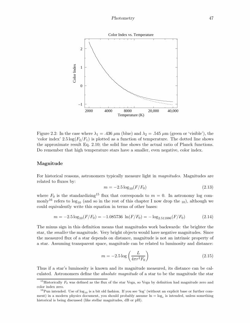
Photometry 47

2000 4000 8000 20,000 40,000

2

1

0

–1

Color Index vs. Temperature

Temperature (K)

Col

or In

dex

Figure 2.2: In the case where λ1 = .436 µm (blue) and λ2 = .545 µm (green or ‘visible’), the‘color index’ 2.5 log(F2/F1) is plotted as a function of temperature. The dotted line showsthe approximate result Eq. 2.10; the solid line shows the actual ratio of Planck functions.Do remember that high temperature stars have a smaller, even negative, color index.

Magnitude

For historical reasons, astronomers typically measure light in magnitudes. Magnitudes arerelated to fluxes by:

m = −2.5 log10(F/F0) (2.13)

where F0 is the standardizing15 flux that corresponds to m = 0. In astronomy log com-monly16 refers to log10 (and so in the rest of this chapter I now drop the 10), although wecould equivalently write this equation in terms of other bases:

m = −2.5 log10(F/F0) = −1.085736 ln(F/F0) = − log2.511886(F/F0) (2.14)

The minus sign in this definition means that magnitudes work backwards: the brighter thestar, the smaller the magnitude. Very bright objects would have negative magnitudes. Sincethe measured flux of a star depends on distance, magnitude is not an intrinsic property ofa star. Assuming transparent space, magnitude can be related to luminosity and distance:

m = −2.5 log

(

L

4πr2F0

)

(2.15)

Thus if a star’s luminosity is known and its magnitude measured, its distance can be cal-culated. Astronomers define the absolute magnitude of a star to be the magnitude the star

15Historically F0 was defined as the flux of the star Vega, so Vega by definition had magnitude zero andcolor index zero.

16Pun intended. Use of log10 is a bit old fashion. If you see ‘log’ (without an explicit base or further com-ment) in a modern physics document, you should probably assume ln = loge is intended, unless somethinghistorical is being discussed (like stellar magnitudes, dB or pH).

48 Photometry

would have if observed from a distance of 10 pc17. Thus:

m = −2.5 log

[

L

4πr2F0

]

(2.16)

= −2.5 log

[

(

L

4π(10 pc)2F0

)

·(

10 pc

r

)2]

(2.17)

= −2.5 log

[

L

4π(10 pc)2F0

]

+ 5 log

[

r

10 pc

]

(2.18)

= M + 5 log

[

r

10 pc

]

(2.19)

whereM is the absolute magnitude and the remaining term: 5 log(r/10 pc) is known as thedistance modulus. The main point here is that distance affects magnitude as a constantoffset. This result is a lemma of the general result:

Theorem: If the measured flux Fm is a fraction (ǫ) of the actual flux F (as wouldoccur due to a less-than-perfectly efficient detector, a dusty mirror, atmospheric absorption,absorption due to interstellar dust,. . . ) the resulting magnitude as measured (mm) is justa constant (2.5 log ǫ) off from the actual magnitude (m).

Proof:

mm = −2.5 log(Fm/F0) (2.20)

= −2.5 log(ǫF/F0) (2.21)

= −2.5 log(F/F0)− 2.5 log(ǫ) (2.22)

= m− 2.5 log(ǫ) (2.23)

In order to calculate flux (W/m2) from photon count rates, we must divide by the photoncollection efficiency, multiply by the energy per photon and divide by the collecting areaof the telescope. But why bother: the above theorem says these multiplicative factorsjust result in a constant offset between the correctly calculated magnitude and one thatsimply ignores these factors. Furthermore, many of these complicating factors (e.g., thefraction of photons absorbed in the atmosphere) cannot be known in advance. Since someof these factors cannot be known in advance, the plan is to ignore all of them (so thecomputer program18 calculating magnitude will not ask you for the energy/photon, quantumefficiency, telescope aperture, etc.), and instead experimentally determine the offset betweenthe computer’s magnitudes (which we will denote in lowercase, e.g., b) and the standardmagnitude (uppercase: B). So part of this lab will involve finding the constant offset thatrelates our measured (instrumental) magnitudes to the actual (standardized) magnitude.

Filters

In the above equation for magnitude, the flux might be the total (all wavelengths or ‘bolo-metric’) light flux, or a monochromatic flux density Fλ, or the flux in a particular rangeof wavelengths. Much of astronomy is concerned with the flux through the five standard19

17pc = parsec = 3.0857 × 1016 m = 3.2616 Ly18gaia magnitudes are calculated as: 50− 2.5 log(gain× net counts/exposure time)19Johnson, H. L. and Morgan, W. W. (1951) ApJ 114 522 & (1953) ApJ 117 313

Cousins, A.W.J. (1976) memRAS 81 25

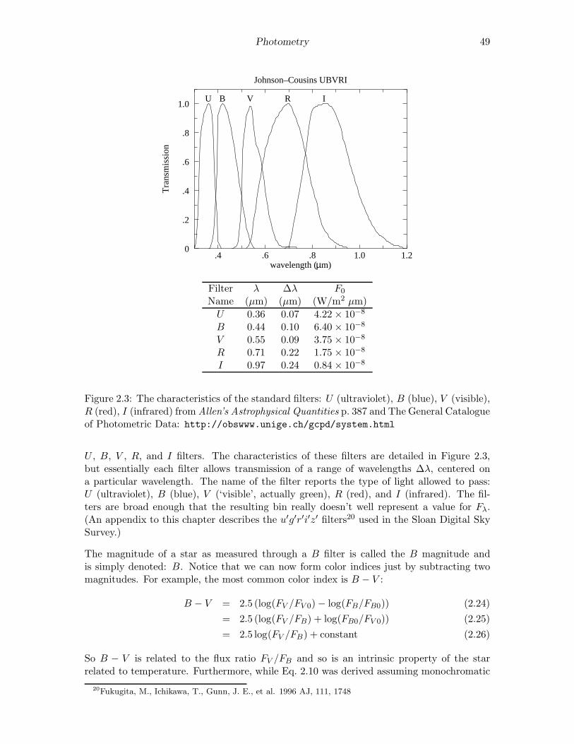
Photometry 49

.4 .6 .8 1.0 1.2

1.0

.8

.6

.4

.2

0

Johnson–Cousins UBVRI

Tra

nsm

issi

on

wavelength ( m)

U B V R I

µ

Filter λ ∆λ F0

Name (µm) (µm) (W/m2 µm)

U 0.36 0.07 4.22× 10−8

B 0.44 0.10 6.40× 10−8

V 0.55 0.09 3.75× 10−8

R 0.71 0.22 1.75× 10−8

I 0.97 0.24 0.84× 10−8

Figure 2.3: The characteristics of the standard filters: U (ultraviolet), B (blue), V (visible),R (red), I (infrared) from Allen’s Astrophysical Quantities p. 387 and The General Catalogueof Photometric Data: http://obswww.unige.ch/gcpd/system.html

U , B, V , R, and I filters. The characteristics of these filters are detailed in Figure 2.3,but essentially each filter allows transmission of a range of wavelengths ∆λ, centered ona particular wavelength. The name of the filter reports the type of light allowed to pass:U (ultraviolet), B (blue), V (‘visible’, actually green), R (red), and I (infrared). The fil-ters are broad enough that the resulting bin really doesn’t well represent a value for Fλ.(An appendix to this chapter describes the u′g′r′i′z′ filters20 used in the Sloan Digital SkySurvey.)

The magnitude of a star as measured through a B filter is called the B magnitude andis simply denoted: B. Notice that we can now form color indices just by subtracting twomagnitudes. For example, the most common color index is B − V :

B − V = 2.5 (log(FV /FV 0)− log(FB/FB0)) (2.24)

= 2.5 (log(FV /FB) + log(FB0/FV 0)) (2.25)

= 2.5 log(FV /FB) + constant (2.26)

So B − V is related to the flux ratio FV /FB and so is an intrinsic property of the starrelated to temperature. Furthermore, while Eq. 2.10 was derived assuming monochromatic

20Fukugita, M., Ichikawa, T., Gunn, J. E., et al. 1996 AJ, 111, 1748

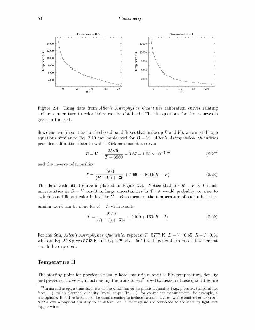
50 Photometry

0 .5 1.0 1.5 2.0

14000

12000

10000

8000

6000

4000

Temperature vs B–V

B–V

Tem

pera

ture

(K

)

0 .5 1.0 1.5 2.0

12000

10000

8000

6000

4000

Temperature vs R–I

R–I

Tem

pera

ture

(K

)

Figure 2.4: Using data from Allen’s Astrophysics Quantities calibration curves relatingstellar temperature to color index can be obtained. The fit equations for these curves isgiven in the text.

flux densities (in contrast to the broad band fluxes that make up B and V ), we can still hopeequations similar to Eq. 2.10 can be derived for B − V . Allen’s Astrophysical Quantitiesprovides calibration data to which Kirkman has fit a curve:

B − V =35800

T + 3960− 3.67 + 1.08 × 10−4 T (2.27)

and the inverse relationship:

T =1700

(B − V ) + .36+ 5060 − 1600(B − V ) (2.28)

The data with fitted curve is plotted in Figure 2.4. Notice that for B − V < 0 smalluncertainties in B − V result in large uncertainties in T : it would probably we wise toswitch to a different color index like U −B to measure the temperature of such a hot star.

Similar work can be done for R− I, with results:

T =2750

(R − I) + .314+ 1400 + 160(R − I) (2.29)

For the Sun, Allen’s Astrophysics Quantities reports: T=5777 K, B − V=0.65, R− I=0.34whereas Eq. 2.28 gives 5703 K and Eq. 2.29 gives 5659 K. In general errors of a few percentshould be expected.

Temperature II

The starting point for physics is usually hard intrinsic quantities like temperature, densityand pressure. However, in astronomy the transducers21 used to measure these quantities are

21In normal usage, a transducer is a device which converts a physical quantity (e.g., pressure, temperature,force,. . . ) to an electrical quantity (volts, amps, Hz . . . ) for convenient measurement: for example, amicrophone. Here I’ve broadened the usual meaning to include natural ‘devices’ whose emitted or absorbedlight allows a physical quantity to be determined. Obviously we are connected to the stars by light, notcopper wires.

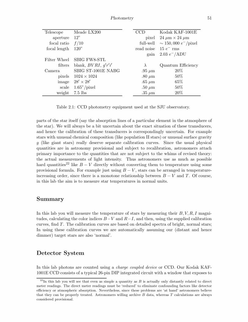
Photometry 51

Telescope Meade LX200aperture 12”

focal ratio f/10focal length 120”

Filter Wheel SBIG FW8-STLfilters blank, BV RI, g′r′i′

Camera SBIG ST-1001E NABGpixels 1024 × 1024image 28′ × 28′

scale 1.65”/pixelweight 7.5 lbs

CCD Kodak KAF-1001Epixel 24 µm× 24 µm

full-well ∼ 150, 000 e−/pixelread noise 15 e− rms

gain 2.03 e−/ADU

λ Quantum Efficiency.95 µm 20%.80 µm 50%.65 µm 65%.50 µm 50%.35 µm 20%

Table 2.1: CCD photometry equipment used at the SJU observatory.

parts of the star itself (say the absorption lines of a particular element in the atmosphere ofthe star). We will always be a bit uncertain about the exact situation of these transducers,and hence the calibration of these transducers is correspondingly uncertain. For examplestars with unusual chemical composition (like population II stars) or unusual surface gravityg (like giant stars) really deserve separate calibration curves. Since the usual physicalquantities are in astronomy provisional and subject to recalibration, astronomers attachprimary importance to the quantities that are not subject to the whims of revised theory:the actual measurements of light intensity. Thus astronomers use as much as possiblehard quantities22 like B − V directly without converting them to temperature using someprovisional formula. For example just using B − V , stars can be arranged in temperature-increasing order, since there is a monotone relationship between B − V and T . Of course,in this lab the aim is to measure star temperatures in normal units.

Summary

In this lab you will measure the temperature of stars by measuring their B,V,R, I magni-tudes, calculating the color indices B−V and R−I, and then, using the supplied calibrationcurves, find T . The calibration curves are based on detailed spectra of bright, normal stars;In using these calibration curves we are automatically assuming our (distant and hencedimmer) target stars are also ‘normal’.

Detector System

In this lab photons are counted using a charge coupled device or CCD. Our Kodak KAF-1001E CCD consists of a typical 26-pin DIP integrated circuit with a window that exposes to

22In this lab you will see that even as simple a quantity as B is actually only distantly related to directmeter readings. The direct meter readings must be ‘reduced’ to eliminate confounding factors like detectorefficiency or atmospheric absorption. Nevertheless, since these problems are ‘at hand’ astronomers believethat they can be properly treated. Astronomers willing archive B data, whereas T calculations are alwaysconsidered provisional.

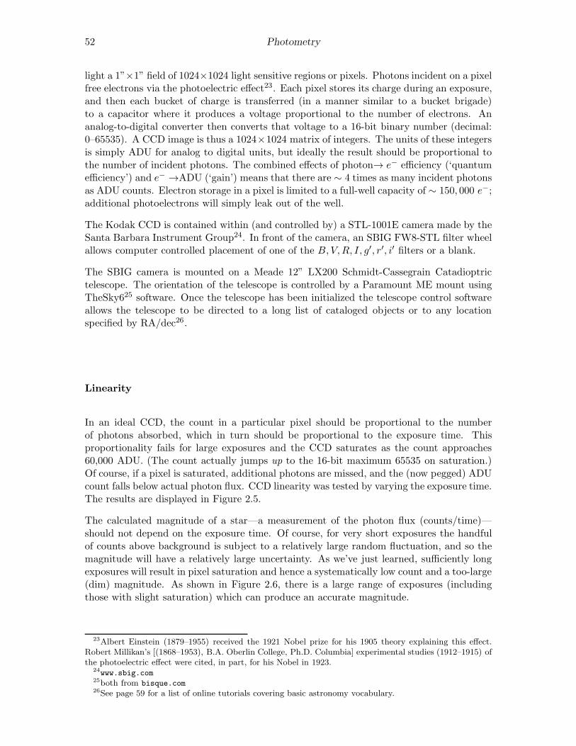
52 Photometry

light a 1”×1” field of 1024×1024 light sensitive regions or pixels. Photons incident on a pixelfree electrons via the photoelectric effect23. Each pixel stores its charge during an exposure,and then each bucket of charge is transferred (in a manner similar to a bucket brigade)to a capacitor where it produces a voltage proportional to the number of electrons. Ananalog-to-digital converter then converts that voltage to a 16-bit binary number (decimal:0–65535). A CCD image is thus a 1024×1024 matrix of integers. The units of these integersis simply ADU for analog to digital units, but ideally the result should be proportional tothe number of incident photons. The combined effects of photon→ e− efficiency (‘quantumefficiency’) and e− →ADU (‘gain’) means that there are ∼ 4 times as many incident photonsas ADU counts. Electron storage in a pixel is limited to a full-well capacity of ∼ 150, 000 e−;additional photoelectrons will simply leak out of the well.

The Kodak CCD is contained within (and controlled by) a STL-1001E camera made by theSanta Barbara Instrument Group24. In front of the camera, an SBIG FW8-STL filter wheelallows computer controlled placement of one of the B,V,R, I, g′, r′, i′ filters or a blank.

The SBIG camera is mounted on a Meade 12” LX200 Schmidt-Cassegrain Catadioptrictelescope. The orientation of the telescope is controlled by a Paramount ME mount usingTheSky625 software. Once the telescope has been initialized the telescope control softwareallows the telescope to be directed to a long list of cataloged objects or to any locationspecified by RA/dec26.

Linearity

In an ideal CCD, the count in a particular pixel should be proportional to the numberof photons absorbed, which in turn should be proportional to the exposure time. Thisproportionality fails for large exposures and the CCD saturates as the count approaches60,000 ADU. (The count actually jumps up to the 16-bit maximum 65535 on saturation.)Of course, if a pixel is saturated, additional photons are missed, and the (now pegged) ADUcount falls below actual photon flux. CCD linearity was tested by varying the exposure time.The results are displayed in Figure 2.5.

The calculated magnitude of a star—a measurement of the photon flux (counts/time)—should not depend on the exposure time. Of course, for very short exposures the handfulof counts above background is subject to a relatively large random fluctuation, and so themagnitude will have a relatively large uncertainty. As we’ve just learned, sufficiently longexposures will result in pixel saturation and hence a systematically low count and a too-large(dim) magnitude. As shown in Figure 2.6, there is a large range of exposures (includingthose with slight saturation) which can produce an accurate magnitude.

23Albert Einstein (1879–1955) received the 1921 Nobel prize for his 1905 theory explaining this effect.Robert Millikan’s [(1868–1953), B.A. Oberlin College, Ph.D. Columbia] experimental studies (1912–1915) ofthe photoelectric effect were cited, in part, for his Nobel in 1923.

24www.sbig.com25both from bisque.com26See page 59 for a list of online tutorials covering basic astronomy vocabulary.

Photometry 53

0 10 20 30

6.E+04

4.E+04

2.E+04

0

Linearity Test

Exposure Time (s)

AD

U

0 1 2 3 4

8000

6000

4000

2000

0

Linearity Test

Exposure Time (s)

AD

U

Figure 2.5: Below ∼ 60, 000 ADU (30 second exposure) the response of our CCD seems tobe linear (reduced χ2 ∼ 1 for errors approximated as

√ADU—generally an overestimate

for error), with saturation evident in the 32 second exposure. (At ∼ 62, 000 ADU thecount jumps up to the 16-bit maximum 65535.) The linear fit even looks good at minimumexposure times where systematic error in the shutter speed control is expected. Note thatthe y intercept is not exactly zero: with this camera zero-time exposures are designed toproduce an output of about 100 ADU.

10 100

42

41

40

39

Saturation

Exposure Time (s)

mag

nitu

de

Figure 2.6: The magnitude of four stars was calculated from frames with various exposures.The brightest two stars have saturated pixels in 20 sec exposures and the dimming mag-nitude is evident in exposures longer than 30 sec. The third brightest star begins to besaturated at 240 sec. The fourth star is not saturated. Notice that a handful of saturatedpixels will generally not result in a large magnitude error.

54 Photometry

Flat Frame

Individual pixels have different sensitivities to light. While the effect is not large (∼ 5%),it would be a leading source of uncertainty if not corrected. The solution is (in theory)simple: take a picture of a uniformly illuminated surface, and record the count in eachpixel. Evidently this ‘flat frame’ count records how each pixel responds to one particularflux level. If in another frame a pixel records some fraction of its flat-frame count, linearityguarantees that the measured flux level is that same fraction of the flat-frame flux level.Thus to correct for varying sensitivities we just divide (pixel by pixel) the raw CCD frameby the flat frame.

In practice it is difficult to obtain a uniformly illuminated surface. In a sky flat, one assumesthat the small section of a blue sky covered in a CCD frame is uniform. (Typically thisis done after sunset so the sky is dim enough to avoid saturation in the short (. 1 sec)exposure, but not so dim that stars show through.) In a dome flat we attempt to uniformlyilluminate a white surface with electric lights. Whatever the source of the flat, it is best toaverage several of them to average out non-uniformities in the source.

It should be clear that a flat frame records the overall efficiency of the system: both thevarying quantum efficiency of individual pixels and the ability of the telescope to gatherlight and concentrate it on a particular pixel. Generally the optical efficiency of a telescopedecreases for sources far from the optical axis. The off-axis limits (where the optical ef-ficiency approaches zero) define a telescope’s maximum field-of-view. The limited opticalefficiency near the edge of the field of view leads to ‘vignetting’: the gradual fade of opticalefficiency to zero at the extreme edge. In addition optical flaws, like dust on optical surfaces,are recorded in a flat frame. As a result a flat frame depends on the entire detection system(telescope, filter, chip) and will gradually change, as for example, dust accumulates on themirror.

Bias Frame

A careful examination of the linearity plots in Figure 2.5, shows that they do not go throughthe origin. That is, a zero-time27 exposure produces some counts, simply by the process ofreading the CCD. The uncertainty in this bias frame (the ‘read noise’) represents the min-imum background noise in any pixel. Measurements on our CCD shows that the differencebetween two bias frames shows an approximately normal distribution (aside from the flaws)with a standard deviation ∼ 11 ADU. Also note that the system artificially introduces anoffset of 100 into each pixel, so 2

3 of the pixels in a single bias frame are expected in the

range 100± 8 ADU. (8 ≈ 11/√2)

Dark Frame

Even in the total absence of light, pixels will slowly accumulate charge. The electric cur-rent leaking into the pixels is strongly affected by temperature, hence the name ‘thermalcurrent’ and it produces accumulated charge in the absence of starlight, hence the name‘dark current’. The professional solution is to cool the CCD using liquid nitrogen, which

27With the STL-1001E the minimum exposure is actually 0.12 s

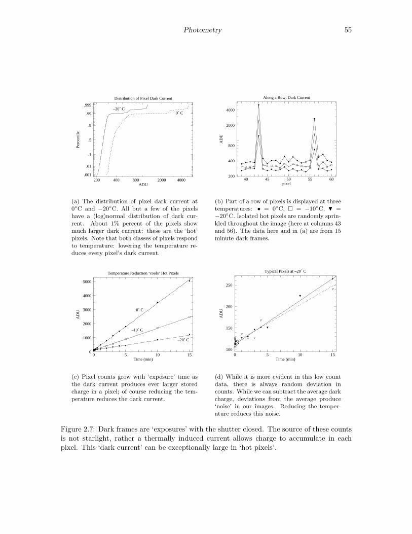
Photometry 55

200 400 800 2000 4000

.999

.99

.9

.5

.1

.01

.001

Distribution of Pixel Dark Current

ADU

Per

cent

ile

–20˚ C0˚ C

(a) The distribution of pixel dark current at0C and −20C. All but a few of the pixelshave a (log)normal distribution of dark cur-rent. About 1% percent of the pixels showmuch larger dark current: these are the ‘hot’pixels. Note that both classes of pixels respondto temperature: lowering the temperature re-duces every pixel’s dark current.

40 45 50 55 60

4000

2000

800

400

200

Along a Row: Dark Current

pixel

AD

U

(b) Part of a row of pixels is displayed at threetemperatures: • = 0C, = −10C, H =−20C. Isolated hot pixels are randomly sprin-kled throughout the image (here at columns 43and 56). The data here and in (a) are from 15minute dark frames.

0 5 10 15

5000

4000

3000

2000

1000

0

Temperature Reduction ‘cools’ Hot Pixels

Time (min)

AD

U 0˚ C

–10˚ C

–20˚ C

(c) Pixel counts grow with ‘exposure’ time asthe dark current produces ever larger storedcharge in a pixel; of course reducing the tem-perature reduces the dark current.

0 5 10 15

250

200

150

100

Typical Pixels at –20˚ C

Time (min)

AD

U

(d) While it is more evident in this low countdata, there is always random deviation incounts. While we can subtract the average darkcharge, deviations from the average produce‘noise’ in our images. Reducing the temper-ature reduces this noise.

Figure 2.7: Dark frames are ‘exposures’ with the shutter closed. The source of these countsis not starlight, rather a thermally induced current allows charge to accumulate in eachpixel. This ‘dark current’ can be exceptionally large in ‘hot pixels’.

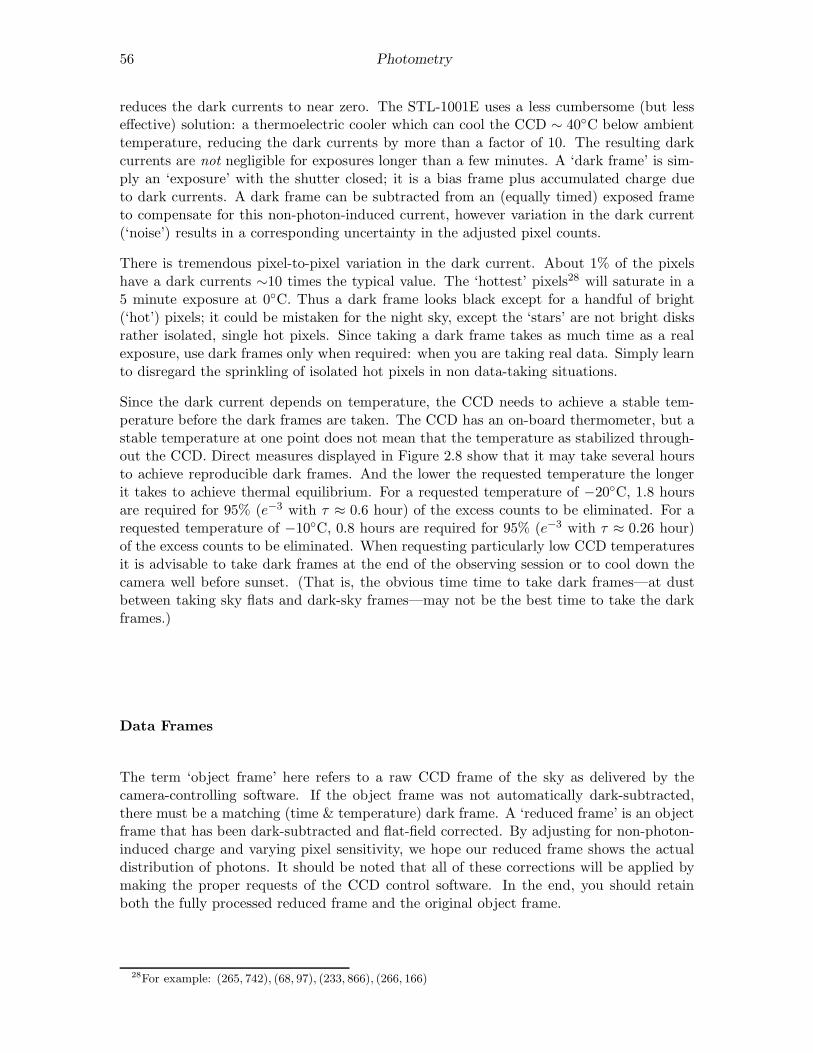
56 Photometry

reduces the dark currents to near zero. The STL-1001E uses a less cumbersome (but lesseffective) solution: a thermoelectric cooler which can cool the CCD ∼ 40C below ambienttemperature, reducing the dark currents by more than a factor of 10. The resulting darkcurrents are not negligible for exposures longer than a few minutes. A ‘dark frame’ is sim-ply an ‘exposure’ with the shutter closed; it is a bias frame plus accumulated charge dueto dark currents. A dark frame can be subtracted from an (equally timed) exposed frameto compensate for this non-photon-induced current, however variation in the dark current(‘noise’) results in a corresponding uncertainty in the adjusted pixel counts.

There is tremendous pixel-to-pixel variation in the dark current. About 1% of the pixelshave a dark currents ∼10 times the typical value. The ‘hottest’ pixels28 will saturate in a5 minute exposure at 0C. Thus a dark frame looks black except for a handful of bright(‘hot’) pixels; it could be mistaken for the night sky, except the ‘stars’ are not bright disksrather isolated, single hot pixels. Since taking a dark frame takes as much time as a realexposure, use dark frames only when required: when you are taking real data. Simply learnto disregard the sprinkling of isolated hot pixels in non data-taking situations.

Since the dark current depends on temperature, the CCD needs to achieve a stable tem-perature before the dark frames are taken. The CCD has an on-board thermometer, but astable temperature at one point does not mean that the temperature as stabilized through-out the CCD. Direct measures displayed in Figure 2.8 show that it may take several hoursto achieve reproducible dark frames. And the lower the requested temperature the longerit takes to achieve thermal equilibrium. For a requested temperature of −20C, 1.8 hoursare required for 95% (e−3 with τ ≈ 0.6 hour) of the excess counts to be eliminated. For arequested temperature of −10C, 0.8 hours are required for 95% (e−3 with τ ≈ 0.26 hour)of the excess counts to be eliminated. When requesting particularly low CCD temperaturesit is advisable to take dark frames at the end of the observing session or to cool down thecamera well before sunset. (That is, the obvious time time to take dark frames—at dustbetween taking sky flats and dark-sky frames—may not be the best time to take the darkframes.)

Data Frames

The term ‘object frame’ here refers to a raw CCD frame of the sky as delivered by thecamera-controlling software. If the object frame was not automatically dark-subtracted,there must be a matching (time & temperature) dark frame. A ‘reduced frame’ is an objectframe that has been dark-subtracted and flat-field corrected. By adjusting for non-photon-induced charge and varying pixel sensitivity, we hope our reduced frame shows the actualdistribution of photons. It should be noted that all of these corrections will be applied bymaking the proper requests of the CCD control software. In the end, you should retainboth the fully processed reduced frame and the original object frame.

28For example: (265, 742), (68, 97), (233, 866), (266, 166)

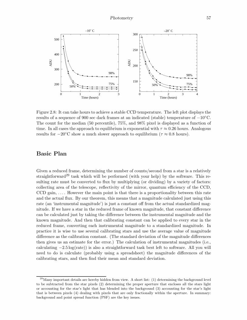
Photometry 57

0 1 2 3

500

400

300

200

–10˚ C

Time (hours)

AD

U

50%75%

98%

0 1 2 3 4

300

250

200

150

–20˚ C

Time (hours)

AD

U

50% 75%

98%

Figure 2.8: It can take hours to achieve a stable CCD temperature. The left plot displays theresults of a sequence of 900 sec dark frames at an indicated (stable) temperature of −10C.The count for the median (50 percentile), 75%, and 98% pixel is displayed as a function oftime. In all cases the approach to equilibrium is exponential with τ ≈ 0.26 hours. Analogousresults for −20C show a much slower approach to equilibrium (τ ≈ 0.8 hours).

Basic Plan

Given a reduced frame, determining the number of counts/second from a star is a relativelystraightforward29 task which will be performed (with your help) by the software. This re-sulting rate must be converted to flux by multiplying (or dividing) by a variety of factors:collecting area of the telescope, reflectivity of the mirror, quantum efficiency of the CCD,CCD gain, . . . . However the main point is that there is a proportionality between this rateand the actual flux. By our theorem, this means that a magnitude calculated just using thisrate (an ‘instrumental magnitude’) is just a constant off from the actual standardized mag-nitude. If we have a star in the reduced frame of known magnitude, that constant differencecan be calculated just by taking the difference between the instrumental magnitude and theknown magnitude. And then that calibrating constant can be applied to every star in thereduced frame, converting each instrumental magnitude to a standardized magnitude. Inpractice it is wise to use several calibrating stars and use the average value of magnitudedifference as the calibration constant. (The standard deviation of the magnitude differencesthen gives us an estimate for the error.) The calculation of instrumental magnitudes (i.e.,calculating −2.5 log(rate)) is also a straightforward task best left to software. All you willneed to do is calculate (probably using a spreadsheet) the magnitude differences of thecalibrating stars, and then find their mean and standard deviation.

29Many important details are hereby hidden from view. A short list: (1) determining the background levelto be subtracted from the star pixels (2) determining the proper aperture that encloses all the stars lightor accounting for the star’s light that has blended into the background (3) accounting for the star’s lightthat is between pixels (4) dealing with pixels that are only fractionally within the aperture. In summary:background and point spread function (PSF) are the key issues.

58 Photometry

at

mos

pher

e

zenth

zL

L sec z

Figure 2.9: Stars that are near zenith go through the minimum amount of the Earth’satmosphere. Stars at a zenith angle z go through sec z times that minimum. This figuredisplays the atmosphere as a finite thickness slab, whereas in fact the atmosphere graduallythins out to nothing. Nevertheless, meter-by-meter a star at angle z must go through sec ztimes as much atmosphere as a star at zenith. ‘Air mass’ is defined as this multiplicativefactor: sec z.

Complications

Air Mass Corrections

Magnitudes are intended to be archivable numbers in which the particulars of the obser-vation (e.g., telescope aperture, quantum efficiency, transparency of the atmosphere,. . . )have been removed. As describe above, this is relatively easy if the reduced frame con-tains calibrated sources. On the other hand, if we have separate reduced frames for theobject and calibrated stars, we must arrange that the entire detection system (atmosphereincluded) acts the same (i.e., the same proportionality constant between rate and flux) forboth frames. However, it is difficult to find calibrated stars that have the same angularaltitude as the object; Thus one frame must be shot through a thicker slice of atmosphericthan the other. Air mass corrections adjust for this path length difference and assume thatthe atmospheres (and optics) were otherwise identical.

The absorption of light is a multiplicative phenomenon; that is, if the first meter of theatmosphere allows fractional transmission of light T1 and the next T2, etc, then the intensityof light through a sequence of meters is:

F = TNTN−1 · · ·T2T1 F0 =

N∏

i=1

Ti F0 (2.30)

Since it is easier to deal with additive quantities rather than multiplicative quantities wedefine the optical depth τ by:

T ≡ e−τ (2.31)

so

F = TNTN−1 · · ·T2T1 F0 = exp

(

−N∑

i=1

τi

)

F0 (2.32)

Photometry 59

According the Beer-Lambert law, the absorption of light depends on atomic absorptivity(the ‘cross section’ σ, which generally depends on the wavelength of light), the number ofatoms per volume (‘number density’ n), and the path length ℓ:

τ = σnℓ (2.33)

We can think of the atmosphere as a sequence of filters, so the light intensity through theatmosphere is:

F = exp

(

−N∑

i=1

σn∆ℓ

)

F0 = exp

(

−∫

σn dℓ

)

F0 (2.34)

Of course the density of the atmosphere (and to some extent the composition of the atmo-sphere) depends on altitude. If we consider light that has taken the shortest path throughthe atmosphere (i.e., from a star directly overhead or at zenith), we call the above integralτ0(λ). (The dependence of τ0 on the wavelength of light is of course due to the dependenceof σ on the wavelength of light.) As shown in Figure 2.9, if a star is at zenith angle z, thepath length (and hence τ) in increased by the air mass factor sec z. Thus:

F = exp (−τ0 sec z)F0 (2.35)

The magnitude that corresponds to this flux is:

m = 2.5τ0 log e sec z +m0 (2.36)

where m is the magnitude measured at zenith angle z and m0 is the magnitude as measuredwithout any atmospheric absorption (i.e., the standardized magnitude). For any singlestar one can (assuming the atmosphere doesn’t change over the few hours required) plot(sec z,m) data as the star rises, culminates and sets, and determine the y-intercept which ism0. Alternatively for a set of stars each with known m0 and measured m at varying sec z,one can determine the correction factors A and B required to convert a star’s (sec z,m) tom0:

m−m0 = B sec z +A (2.37)

Thus lacking in-frame calibrated stars, several calibration frames (at different sec z) arerequired for each filter, and the reduction process becomes much more complicated.

Note that the zenith angle z can be calculated30 from:

cos z = sin δ sinϕ+ cos δ cos h cosϕ (2.38)

where δ and h are the star’s declination and hour angle and ϕ is the observatory’s latitude.The above terms from astrometry (declination, hour angle, altitude, zenith, right ascension,. . . ) are part of the everyday vocabulary of astronomers. If you are not familiar with theseterms you should read the following online tutorials:

• http://www.physics.csbsju.edu/astro/CS/CSintro.html

• http://www.physics.csbsju.edu/astro/sky/sky.01.html

• http://www.physics.csbsju.edu/astro/terms.html

For example at SJU (ϕ = 4534.5′) for stars on the celestial equator (δ = 0), the minimumair mass (at h = 0h) is sec z = 1.43. The sequence of air masses: sec z=1.5, 2.0, 2.5, 3.0occurs at hour angles h = ±1.18h,±2.96h,±3.68h,±4.10h. Figure 2.11 plots these air massvalues for other declinations.

30xephem can do this calculation for you

60 Photometry

1.8 2.0 2.2 2.4 2.6 2.8

31.20

31.15

31.10

31.05

31.00

Air Mass

v–V

Figure 2.10: The instrumental magnitude minus the standardized magnitude (v − V ) for ared star () and a blue star () as a function of the air mass. Notice that the slopes arequite similar (i.e., .177 sec z), but the intercepts are slightly different (∆ = 0.016(B − V )),due to the difference in color. This color correction is explained in the following section.The rms deviation in these fits is 0.005 magnitudes which is about 1

3 the intercept shift.

–8 –6 –4 –2 0 2 4 6 8

60

40

20

0

–20

Air Mass

Hour Angle

Dec

linat

ion

1.1 1.2 1.5 2.0 2.5

3.0

Z

Figure 2.11: Air mass (sec z) depends on where a star is in the sky. Air mass is plotted hereas a function of the star’s declination and hour angle for the SJU observatory location. Zmarks zenith, where the minimum (1) air mass is found.

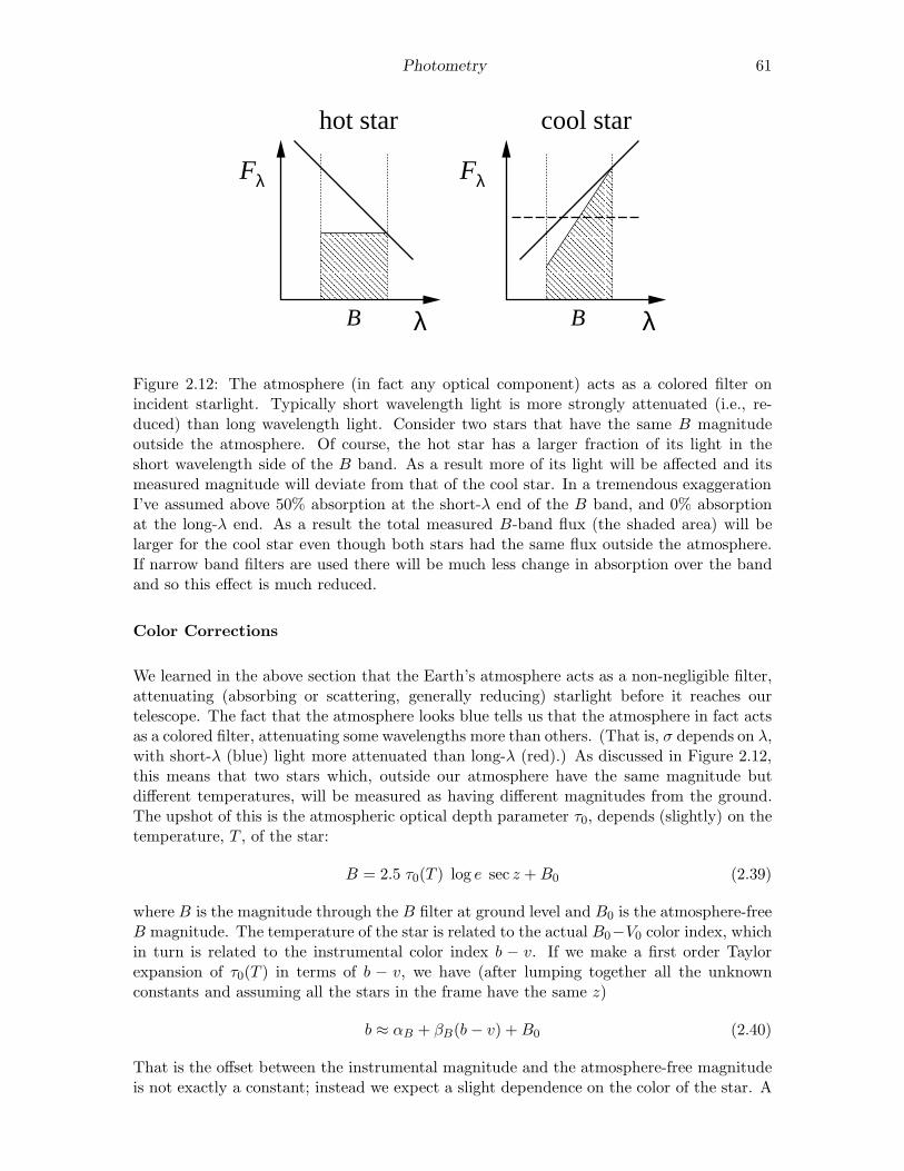
Photometry 61

Fλ Fλ

λλ

hot star cool star

B B7777777777777777777777777777777777777777777777777777777777777777

7777777777777777777777777777777777777777777777777777777777777777777777777777777777777777777777777777777777777777

Figure 2.12: The atmosphere (in fact any optical component) acts as a colored filter onincident starlight. Typically short wavelength light is more strongly attenuated (i.e., re-duced) than long wavelength light. Consider two stars that have the same B magnitudeoutside the atmosphere. Of course, the hot star has a larger fraction of its light in theshort wavelength side of the B band. As a result more of its light will be affected and itsmeasured magnitude will deviate from that of the cool star. In a tremendous exaggerationI’ve assumed above 50% absorption at the short-λ end of the B band, and 0% absorptionat the long-λ end. As a result the total measured B-band flux (the shaded area) will belarger for the cool star even though both stars had the same flux outside the atmosphere.If narrow band filters are used there will be much less change in absorption over the bandand so this effect is much reduced.

Color Corrections

We learned in the above section that the Earth’s atmosphere acts as a non-negligible filter,attenuating (absorbing or scattering, generally reducing) starlight before it reaches ourtelescope. The fact that the atmosphere looks blue tells us that the atmosphere in fact actsas a colored filter, attenuating some wavelengths more than others. (That is, σ depends on λ,with short-λ (blue) light more attenuated than long-λ (red).) As discussed in Figure 2.12,this means that two stars which, outside our atmosphere have the same magnitude butdifferent temperatures, will be measured as having different magnitudes from the ground.The upshot of this is the atmospheric optical depth parameter τ0, depends (slightly) on thetemperature, T , of the star:

B = 2.5 τ0(T ) log e sec z +B0 (2.39)

where B is the magnitude through the B filter at ground level and B0 is the atmosphere-freeB magnitude. The temperature of the star is related to the actual B0−V0 color index, whichin turn is related to the instrumental color index b − v. If we make a first order Taylorexpansion of τ0(T ) in terms of b − v, we have (after lumping together all the unknownconstants and assuming all the stars in the frame have the same z)

b ≈ αB + βB(b− v) +B0 (2.40)

That is the offset between the instrumental magnitude and the atmosphere-free magnitudeis not exactly a constant; instead we expect a slight dependence on the color of the star. A

62 Photometry

FWHM

FWHM

bright stardim star

pixel

AD

U

Figure 2.13: Every photon detected in a CCD frame has traversed (essentially) the samepatch of atmosphere, so each star’s image suffers the same distortion. Every stellar ‘image’(really point spread function or PSF) has the same shape, only the total flux in each imagevaries (with the star’s magnitude). However, a brief inspection of an image will show clearlylarger spots for brighter stars. As shown above this is simply a matter of the level chosenas bright.

linear fit (using the data from the calibrated sources) can then be used to determine α andβ, viz:

b−B0 = αB + βB(b− v) (2.41)

and similarly for the V magnitudes:

v − V0 = αV + βV (b− v) (2.42)

Subtracting these two equations gives us the relationship between the instrumental colorindex and the atmosphere-free color index:

(b− v)− (B0 − V0) = αB − αV + (βB − βV )(b− v) (2.43)

[1 + (βV − βB)] (b− v) + (αV − αB) = B0 − V0 (2.44)

Thus we expect a linear relationship (with a nearly unit slope) between the instrumentalcolor index and the atmosphere-free color index. The parameters of this linear relationshipcan be determined by a fit using the data from the calibrated stars.

Aperture Corrections

When you look at your CCD frames, you will not believe my statement that all the starimages (really PSF) have the same size. However, both bright stars and dim stars are farenough away that their angular diameters are effectively zero (less than a thousandth of asingle pixel). The photons from each star shoot through the Earth’s atmosphere and are

Photometry 63

deflected this way and that producing a multi-pixel disk in the frame. This is called atmo-spheric seeing (particularly for image size) or scintillation (particularly for image bright-ness). But since every photon is shot (basically) through the same patch of atmosphere,these random deflections must have the same distribution. The difference between a dimstar and a bright star is simply the total number of photons in the images. (That is a longtime exposure of a dim star should look exactly31 like a short exposure of a bright starif the two cases produce the same number of photons.) To see that the distributions areidentical you should look at the full width at half maximum (FWHM) of the PSF: Firstdetermine the peak count in an image, and then find the circle at which the count is halfof this maximum. The diameter of the circle (typically a few arcsec) is the FWHM.

Because of the obvious difference in the image size, when totaling the counts in a stellarimage, one is tempted to expand or reduce the circle of pixels counted as part of a star tomatch the apparent size of that star. Do not do this! Instead keep a constant aperture sizefor all frames. It may appear that counts will be missed as bright stars overflow the aperture,whereas dim stars have a too-large aperture. However recall that all stars actually have thesame extent. Furthermore our theorem states that if we capture a consistent fraction of thecounts in every star, all our instrumental magnitudes will just be a constant off from thestandardized magnitudes. So a consistent fraction of the counts may be combined with allthe other proportionality constants in the final difference between instrumental magnitudeand standardized magnitude. Now there may be occasions where we must adjust the aper-ture used for magnitude calculation (for example to exclude a neighboring star), howeverthen inconsistencies (and hence errors) are then being generated. The disadvantage of usinga constant aperture is relatively more noise-prone ‘background’ pixels will be included indim stars. There are a variety of solutions to this problems (generally under the heading ofPSF fitting), however they are beyond the aims of this lab.

The blurring of star images (i.e., PSF) depends both on atmospheric seeing and the ad-justment of the telescope. Clearly an out-of-focus telescope (see below) will distribute thesame photons in a larger radius disk. It should also be noted that the telescope’s ‘opticalaberrations’ result in additional blurring (‘coma’) near the edge of the telescope’s field ofview.

Focus

The aim of focus is to achieve that smallest possible FWHM, so each star’s light is con-centrated in the fewest possible number of pixels. Same number of photons in fewer pixels,means a higher count in those central pixels. Since every pixel comes with a certain back-ground ‘noise’, fewer pixels means less noise in the stellar magnitude. You should plan onspending a good bit of time (maybe a half hour) trying to achieve the best possible focus.There are two approaches to monitoring improved focus: (1) monitor the peak count in abright star (∼ 4 mag), (2) watch for the appearance of numerous dim stars as their peakgets above the ‘bright’ level. (You must learn to ignore the apparent size of bright stars:it is a poor measure of good focus.) A complicating factor is that both (1) and (2) varyindependently of focus adjustments since atmospheric seeing varies from second to second,and since photon counts should be expected to vary ∼

√N .

31We are assuming, of course, that the atmosphere acts the same during the long exposure as it doesduring the short exposure. No surprise: in fact the atmosphere is not time-invariant.

64 Photometry

Software

xephem

xephem is planetarium software designed to display various types of night-sky maps inadvance of observing. You will also use it to tabulate astrometry data relevant to yourobservations. The file using.xephem.txt describes how to use this program to produce thetables and maps required for the pre-observation phase of the lab. In addition you can useit for astrometry and photometry on .fit images (although I recommend gaia below forthese reductions).

Aladin

Aladin is a front-end to various astronomy databases on the internet. You will use it tofind images to use as finder maps and to identify (and obtain data on ) the stars in thoseimages. The Aladin server and SkyView+ are often a good sources of images; Simbad32 isthe usual source for stellar information. Sometimes just information from the SAO catalogis required; then VizieR33 can be used to access just the SAO catalog. You will use Aladinmostly in the pre-observation phase. The file using.Aladin.txt briefly describes how touse this program to produce the maps and data required for the pre-observation phase ofthe lab. Note: NASA has a very handy web page34 that also allows you to do many of thesethings. gaia (see below) is also and excellent way to make finder maps.

CCDops

CCDOps is software used to control the camera and create/save CCD frames. You will beusing a small fraction of its capabilities. Typical commands will be: to set the tempera-ture (cooling) of the CCD, focus, grab images (set the exposure time and perhaps take adark frame), examine images (histogram, crosshair), save images (in both .SBIG and .fit

formats), and reduce images by dark-subtracting, flat-fielding or averaging.

gaia

gaia is the recommended reduced-frame analysis program. In order to use gaia your imagesmust be in either .fit or ndf (.sdf) format. You can convert your .SBIG frame into andf frame (.sdf) using the program sbig2ndf or the many-files script batch ndf, but itis easier to directly save your images in .fit format. The file using.gaia.txt brieflydescribes how to use this program.

In addition to reporting a star’s magnitude, gaia will report the error in that magnitude.This error is based on counting (Poisson statistics,

√N). These errors will be smaller for

brighter stars; a typical value might be ∼ 0.003. Record one typical gaia-reported error

32http://simbad.u-strasbg.fr/33http://vizier.u-strasbg.fr/34http://skyview.gsfc.nasa.gov/: start with 1000×1000 pixel Digitized Sky Survey image with 0.5

Image Size, B-W Log Inverse Color Table, and a Grid

Photometry 65

for your stars. Because of systematic errors, you will find the actual error is much larger∼ 0.02.

IRAF

IRAF is the Image Reduction and Analysis Facility, a general purpose software systemfor the reduction and analysis of astronomical data. It is the standard for professionalastronomers: designed for the expert user—with no compromises for the beginner. Whileits use is encouraged for those thinking of becoming astronomers, I cannot recommend itfor this lab.

Planning to Observe

Minnesota weather is is unpredictable35 and we need an extraordinary, no-visible-cloudsnight. We must be prepared to use any/every of these rare nights on short notice. Ofcourse, you have other commitments (your concert, the night before your math/physicsexam, the St. Thomas game. . . ), the aim here is to communicate those constraints to meand to your lab partners in well in advance. Thus you will need to carefully record yourschedule a lunar month ahead. Note that Murphy’s Law guarantees that if you forget toX-out some important night (your girlfriend’s birthday, the day before your term paper isdue, a ‘free’ day), that night will be clear, and somebody (I hope not me!) is going tobe disappointed. My family commitments and intro astro labs are going X-out all Sundaynights and many Monday and Wednesday nights.

Before each full moon, mark on the class calendar the dates you and your lab partner(s)are committed to observe.

Since clear nights are precious, ‘go’ days need a well-thought-out plan. If you’re followingthe standard project, your plan involves a target whose frame will include several starswith known36 B,V,R, I magnitudes. Thus you need to: (A) Find a target that has therequired stars. (Stars with recorded R magnitudes are relatively rare.) (B) Know wherethose standard stars are in your target (so you can aim so your CCD frames to include thestars you need). (C) Know where your target is among the neighboring stars (so if yourfirst try at finding the target fails, you have a plan [not ‘hunt-and-peck’] for getting to theright spot). (D) And of course, know that your target is well above the horizon when youare planning to observe. While the standard project does not require additional standardstars, you may want you to record alternative (out-of-frame) standards.

Thus, you must produce (and turn in) the pre-observation documents described below.Using the following new moon as a date, use xephem, to select your targets. The problem isto find a star cluster that has the required calibrated stars. For spring, M 67 is the obviouschoice, but any cluster listed in Table 2.2 before M 67 should also be above the horizon.

35http://www.physics.csbsju.edu/astro/ has a link designed to report (guess) sky conditions at theSJU observatory. It cannot be relied on, but I believe it’s the best available information. Note: black isgood for this clear sky clock.

36Professionally, only very carefully measured ‘standard’ stars—for example those measured by Landoltor Stetson—would be used for calibration. For the purposes of this lab you may use any star that has a‘book’ magnitude. It is not at all unusual for such literature magnitudes to have 10% errors

66 Photometry

Pre-observation Checklist

The following should be prepared before each full moon (2-Feb-11, 4-Mar-11, 3-Apr-11):

1. Sign up for ‘go’ days during the following lunar month.

2. Using xephem set for the date of the following new moon print out the following:

(a) A Sky View showing the entire sky with the labeled location of the target.It is helpful to label the brightest stars with the Meade * number from theMeade250.edb file.

(b) A .xephem/datatbl.txt file recording basic data (RA, dec, altitude, air mass,. . . ) for the target at the suggested observation time.

(c) A copy&pasted list of basic data on the stars (e.g., from SAO LX200.edb) usedto locate the target and perhaps selected standard stars. At least one nearby starshould be a ‘focus star’ with mag ∼3–5. The file using.xephem.txt describeswhat data you need to have recorded.

3. Using Aladin (or web-based skyview.gsfc.nasa.gov) print out the following findingcharts for your target cluster:

(a) a low magnification (degree scale) image showing both a finder LX200 star andthe desired CCD frame.

(b) an image scaled to about the CCD frame size (0.5) showing exactly the desiredCCD frame. (Since the target CCD frame must include calibrated stars, clearlyyou must know where the calibrated stars are in the target.) Record the RA anddec for your target frame(s).

Learning to effectively use these pre-observation programs will be a bit of a challenge andtake several hours, so do not procrastinate and feel free to seek my help. In addition to theusual problems of learning new software, you will need to learn how to make the web-basedastronomy databases find the information you need.

Example 1: Plan for Lunar Month starting 21-July-2005

Immediately on starting xephem, Set the location: SJU Observatory, click on the Calendarfor the following new moon (“NM”, in this case 4-August-2005) and enter a Local Time of21:00 (9 p.m.). Hit Update so xephem is ready to display the sky at that time. View→SkyView then displays the night sky for that location/date/time. (Print a copy of this sky viewas described in using.xephem.txt and record: UTC Time: 2:00, Sidereal: 16:37.) IC 4665is the obvious target; its RA (listed in Table 2.2) is most nearly equal to the sidereal timeand hence it is near the meridian, However, with a diameter of 70′, IC 4665 is much largerthan the ST7 CCD frame, so only a small fraction of it will be imaged—a fraction that mustinclude several calibrated stars. A visit to the IC 4665 cluster web page37 finds a couple ofdozen of VRIc observations. I copy and paste that data into a spreadsheet, and then seekcorresponding UBV CCD data. The result is 12 stars with the full set of BV RI data. Next

37http://obswww.unige.ch/webda/

Photometry 67

we need to find a CCD frame that will include as many of these stars as possible. (It is ofcourse possible to use a different set of stars to calibrate different filters, but it will be easierif one set of stars will serve for all calibrations.) Surprisingly, most of the 12 stars haveSAO38 identifications; only three stars must be located by RA and dec. Aladin can find alow magnification (1.5 × 1.5) image of IC 4665. (Print this image as a low magnificationfinder chart.) A request to VizieR for the SAO catalog objects near IC 4665 allows meto locate the calibrated sources found above. Since IC 4665 is much larger than our CCDframe, we aim for the largest possible subset of these stars. A CCD frame centered nearSAO 122742 will pick up four fully calibrated stars (73, 82, 83, 89). Simbad gives B−V datafor several other bright stars in this frame (e.g., TYC 424-75-1, Cl* IC4665 P44), but I don’tfind additional R−I data in Simbad. Returning to obswww.unige.ch, I find (depending onthe exact position of the CCD frame) it may be possible to include R − I calibrated stars67, 76, 84, & 90. You should decide exactly how to place the CCD frame and locate thecalibrated stars on a finder chart that is about 2× the size of the CCD frame. For focusstars consider SAO 122671 (mag=3) and SAO 123005 (mag=5). Note that SAO 122723would make a good (bright: mag=6.8) star to aim the LX200 near this object. (I callsuch aiming/finding stars ‘LX200 stars’. The LX200 object library includes all SAO starsbrighter than magnitude 7, but any bright star can help assure the telescope is aimed atwhat you intend (and that the telescope’s reported RA/dec are accurate). You can load theSAO LX200.edb database into xephem to display the LX200 stars; SAO mag75.edb includesabout twice as many stars (down to magnitude 7.5); SAO full.edb includes about a quarterof a million stars (down below magnitude 9).

In such a large cluster, it would be wise to select additional fields, for example one centerednear SAO 122709. A CCD frame there might include R− I calibrated stars: 39, 40, 43, 44,49, 50, 58, 62.

To select alternative standards. . .WIYN has a web page39 with recommended standard starregions. (WIYN’s stars are designed for a large telescope, and hence would require longexposures on our telescope). Peter Stetson’s extensive list of standards is also online40.The xephem databases LONEOS.edb, Landolt83.edb and Buil91.edb contain shorter listsof brighter stars: < 13mag, ∼9.5mag and < 8mag respectively.) Generally these goodstandard stars will be well-separated from the target, so air mass air mass correction wouldbe required. (Since I have internal ‘calibrated’ sources, I’m not required to take CCD framesof these standards, however I’ve decided to ‘be prepared’ and hence have recorded the basicdata I would need to observe them.) I select: #109 (PG1633+099, at RA=16:35, LX200star: SAO 121671), #121 (110 506, at RA=18:43, LX200 star: SAO 142582), and #125(111 1969, at RA=19:37, LX200 star: SAO 143678, also see: SAO 124878). These standardstars can be marked as xephem Favorites from the UBVRI.edb database. These sourcesshould span a good range of air mass in the general direction of the target. Following theinstructions in using.xephem.txt, I create a file of basic location data for my target andstandard fields. By default, this file is: .xephem/datatbl.txt and can be printed (% lp

filename) or edited (% kwrite filename).

38Smithsonian Astrophysical Observatory—a standard catalog of ‘bright’ stars.39http://www.noao.edu/wiyn/obsprog/images/tableB.html40http://cadcwww.hia.nrc.ca/standards

68 Photometry

Example 2: Plan for Lunar Month starting 19-August-2005

After Setting xephem for location: SJU Observatory, the new moon date 3-September-2005, and Local Time 21:00 (9 p.m.), I find and record: UTC Time: 2:00, Sidereal: 18:35.NGC 6633, whose RA is most nearly equal to the sidereal time and hence is near themeridian, is the obvious target. After adding NGC 6633 to xephem Favorites and loading theSAO database (Data→Files; Files→SAO mag75.edb), it’s easy to zoom in (lhs scroll bar) onNGC 6633 and find the nearby bright (5.7 mag) star SAO 12351641 , which would be a goodstar to steer the LX200. For focus stars consider SAO 122671 (mag=3) and SAO 123377(mag=5). A visit to the NGC 6633 cluster web page42 finds six VRIe observations for R.Cross-reference shows that all six are ∼ 8 mag SAO stars43, however only two (50 & 70) arein the central region of the cluster. (They could also be found using SAO full.edb.) Stetsonreports BV I data for NGC 6633, however the brightest ten of his stars are ∼ 13 mag,which is 100× dimmer than the ∼ 8 mag R-mag stars. Thus different frames are requiredto properly expose the Stetson standards and the R ‘standards’.

Using the Buil91.edb database, I can find bright standard stars: SAO 085402, SAO 141956,SAO 145050. These bright SAO stars are themselves LX200 stars.

Example 3: Plan for Lunar Month starting 21-June-2005

After Setting xephem for location: SJU Observatory, the new moon date 6-July-2005, andLocal Time 22:00 (10 p.m. — it’s not dark at 9 p.m.), I find and record: UTC Time: 3:00,Sidereal: 15:43. Because of its larger declination, Upgren 1 has a bit less air mass thanNGC 6633, so it becomes the target. Upgren 1 is not in xephem’s databases, so it must beadded to Favorites following the procedure recorded in using.xephem.txt. A visit to theUpgren 1 cluster web page44 finds seven stars with VRIc and UBV observations. Howeverthe color index disagreements are of order 0.05, so we can use this as an opportunity to findthe correct values. Using the Landolt83.edb database, I find three neighboring standardstars with a range of colors: HD 102056 (LX200 star: SAO 81968, bluer than the Upgren1 stars), HD 106542 (LX200 star: SAO 100009, redder than the Upgren 1 stars), andHD 107146 (LX200 star: SAO 100038, similar to the Upgren 1 stars). Using the Oja96.edbdatabase, I find two very close stars with similar colors: BD+35 2356 and BD+34 2338.(For these dimmer, ∼10 magnitude, stars finder charts are required.) ∗#133 (SAO 63257,with mag 5 partner 63256) is a neighboring mag 3 star, SAO 44230 is a mag 4 star — bothcan help focus and alignment. SAO 63118 is the nearest LX200 star to Upgren 1 (sinceUpgren 1 is not in the LX200 catalog of clusters, the final jump must be made based onRA/dec). All but one of the Upgren 1 seven stars is an SAO star; they are all easy toidentify with Aladin. (FYI: spiral galaxies M94 and M63 might be worth a look.)

Target and standards were fairly close together and near the meridian during the measure-ments, with airmass varying from 1.01 to 1.14. This was not a sufficient range to detectairmass correction terms. Increasing airmass dims and reddens stars. As a result calibratedstars viewed through a larger air mass will have a smaller constant in the color calibration

41VizieR reports R = 5.703, for this star, which may serve as an additional standard. FYI: this star isalso known as: HD 170200 and HR 6928.

42Again: http://obswww.unige.ch/webda/43These dim SAO stars are not in SAO mag75.edb so I located them using Aladin44Again: http://obswww.unige.ch/webda/

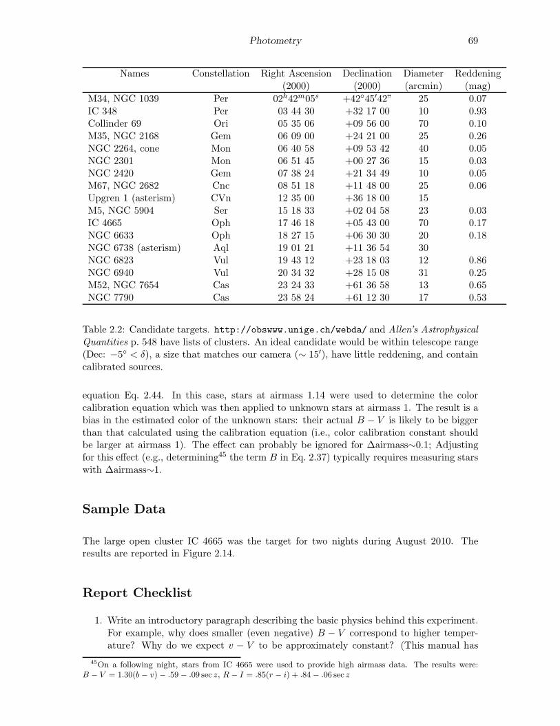
Photometry 69

Names Constellation Right Ascension Declination Diameter Reddening(2000) (2000) (arcmin) (mag)

M34, NGC 1039 Per 02h42m05s +4245′42” 25 0.07IC 348 Per 03 44 30 +32 17 00 10 0.93Collinder 69 Ori 05 35 06 +09 56 00 70 0.10M35, NGC 2168 Gem 06 09 00 +24 21 00 25 0.26NGC 2264, cone Mon 06 40 58 +09 53 42 40 0.05NGC 2301 Mon 06 51 45 +00 27 36 15 0.03NGC 2420 Gem 07 38 24 +21 34 49 10 0.05M67, NGC 2682 Cnc 08 51 18 +11 48 00 25 0.06Upgren 1 (asterism) CVn 12 35 00 +36 18 00 15M5, NGC 5904 Ser 15 18 33 +02 04 58 23 0.03IC 4665 Oph 17 46 18 +05 43 00 70 0.17NGC 6633 Oph 18 27 15 +06 30 30 20 0.18NGC 6738 (asterism) Aql 19 01 21 +11 36 54 30NGC 6823 Vul 19 43 12 +23 18 03 12 0.86NGC 6940 Vul 20 34 32 +28 15 08 31 0.25M52, NGC 7654 Cas 23 24 33 +61 36 58 13 0.65NGC 7790 Cas 23 58 24 +61 12 30 17 0.53

Table 2.2: Candidate targets. http://obswww.unige.ch/webda/ and Allen’s AstrophysicalQuantities p. 548 have lists of clusters. An ideal candidate would be within telescope range(Dec: −5 < δ), a size that matches our camera (∼ 15′), have little reddening, and containcalibrated sources.

equation Eq. 2.44. In this case, stars at airmass 1.14 were used to determine the colorcalibration equation which was then applied to unknown stars at airmass 1. The result is abias in the estimated color of the unknown stars: their actual B − V is likely to be biggerthan that calculated using the calibration equation (i.e., color calibration constant shouldbe larger at airmass 1). The effect can probably be ignored for ∆airmass∼0.1; Adjustingfor this effect (e.g., determining45 the term B in Eq. 2.37) typically requires measuring starswith ∆airmass∼1.

Sample Data

The large open cluster IC 4665 was the target for two nights during August 2010. Theresults are reported in Figure 2.14.

Report Checklist

1. Write an introductory paragraph describing the basic physics behind this experiment.For example, why does smaller (even negative) B − V correspond to higher temper-ature? Why do we expect v − V to be approximately constant? (This manual has

45On a following night, stars from IC 4665 were used to provide high airmass data. The results were:B − V = 1.30(b − v)− .59− .09 sec z, R − I = .85(r − i) + .84− .06 sec z

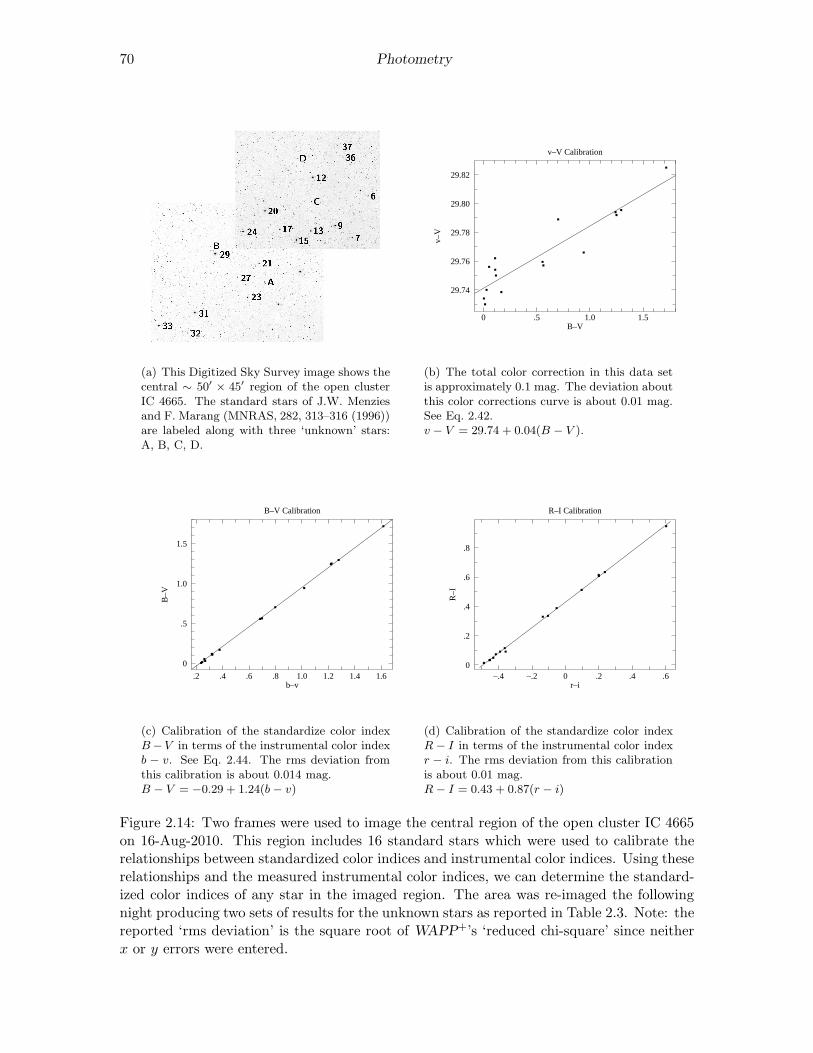
70 Photometry

(a) This Digitized Sky Survey image shows thecentral ∼ 50′ × 45′ region of the open clusterIC 4665. The standard stars of J.W. Menziesand F. Marang (MNRAS, 282, 313–316 (1996))are labeled along with three ‘unknown’ stars:A, B, C, D.

0 .5 1.0 1.5

29.82

29.80

29.78

29.76

29.74

v–V Calibration

B–V

v–V

(b) The total color correction in this data setis approximately 0.1 mag. The deviation aboutthis color corrections curve is about 0.01 mag.See Eq. 2.42.v − V = 29.74 + 0.04(B − V ).

.2 .4 .6 .8 1.0 1.2 1.4 1.6

1.5

1.0

.5

0

B–V Calibration

b–v

B–V

(c) Calibration of the standardize color indexB−V in terms of the instrumental color indexb − v. See Eq. 2.44. The rms deviation fromthis calibration is about 0.014 mag.B − V = −0.29 + 1.24(b − v)

–.4 –.2 0 .2 .4 .6

.8

.6

.4

.2

0

R–I Calibration

r–i

R–I

(d) Calibration of the standardize color indexR − I in terms of the instrumental color indexr − i. The rms deviation from this calibrationis about 0.01 mag.R − I = 0.43 + 0.87(r − i)

Figure 2.14: Two frames were used to image the central region of the open cluster IC 4665on 16-Aug-2010. This region includes 16 standard stars which were used to calibrate therelationships between standardized color indices and instrumental color indices. Using theserelationships and the measured instrumental color indices, we can determine the standard-ized color indices of any star in the imaged region. The area was re-imaged the followingnight producing two sets of results for the unknown stars as reported in Table 2.3. Note: thereported ‘rms deviation’ is the square root of WAPP+’s ‘reduced chi-square’ since neitherx or y errors were entered.

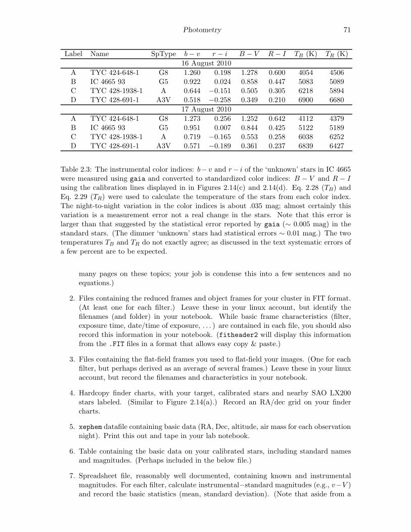
Photometry 71

Label Name SpType b− v r − i B − V R− I TB (K) TR (K)

16 August 2010

A TYC 424-648-1 G8 1.260 0.198 1.278 0.600 4054 4506B IC 4665 93 G5 0.922 0.024 0.858 0.447 5083 5089C TYC 428-1938-1 A 0.644 −0.151 0.505 0.305 6218 5894D TYC 428-691-1 A3V 0.518 −0.258 0.349 0.210 6900 6680

17 August 2010

A TYC 424-648-1 G8 1.273 0.256 1.252 0.642 4112 4379B IC 4665 93 G5 0.951 0.007 0.844 0.425 5122 5189C TYC 428-1938-1 A 0.719 −0.165 0.553 0.258 6038 6252D TYC 428-691-1 A3V 0.571 −0.189 0.361 0.237 6839 6427

Table 2.3: The instrumental color indices: b− v and r− i of the ‘unknown’ stars in IC 4665were measured using gaia and converted to standardized color indices: B − V and R − Iusing the calibration lines displayed in in Figures 2.14(c) and 2.14(d). Eq. 2.28 (TB) andEq. 2.29 (TR) were used to calculate the temperature of the stars from each color index.The night-to-night variation in the color indices is about .035 mag; almost certainly thisvariation is a measurement error not a real change in the stars. Note that this error islarger than that suggested by the statistical error reported by gaia (∼ 0.005 mag) in thestandard stars. (The dimmer ‘unknown’ stars had statistical errors ∼ 0.01 mag.) The twotemperatures TB and TR do not exactly agree; as discussed in the text systematic errors ofa few percent are to be expected.

many pages on these topics; your job is condense this into a few sentences and noequations.)

2. Files containing the reduced frames and object frames for your cluster in FIT format.(At least one for each filter.) Leave these in your linux account, but identify thefilenames (and folder) in your notebook. While basic frame characteristics (filter,exposure time, date/time of exposure, . . . ) are contained in each file, you should alsorecord this information in your notebook. (fitheader2 will display this informationfrom the .FIT files in a format that allows easy copy & paste.)

3. Files containing the flat-field frames you used to flat-field your images. (One for eachfilter, but perhaps derived as an average of several frames.) Leave these in your linuxaccount, but record the filenames and characteristics in your notebook.

4. Hardcopy finder charts, with your target, calibrated stars and nearby SAO LX200stars labeled. (Similar to Figure 2.14(a).) Record an RA/dec grid on your findercharts.

5. xephem datafile containing basic data (RA, Dec, altitude, air mass for each observationnight). Print this out and tape in your lab notebook.

6. Table containing the basic data on your calibrated stars, including standard namesand magnitudes. (Perhaps included in the below file.)

7. Spreadsheet file, reasonably well documented, containing known and instrumentalmagnitudes. For each filter, calculate instrumental−standard magnitudes (e.g., v−V )and record the basic statistics (mean, standard deviation). (Note that aside from a

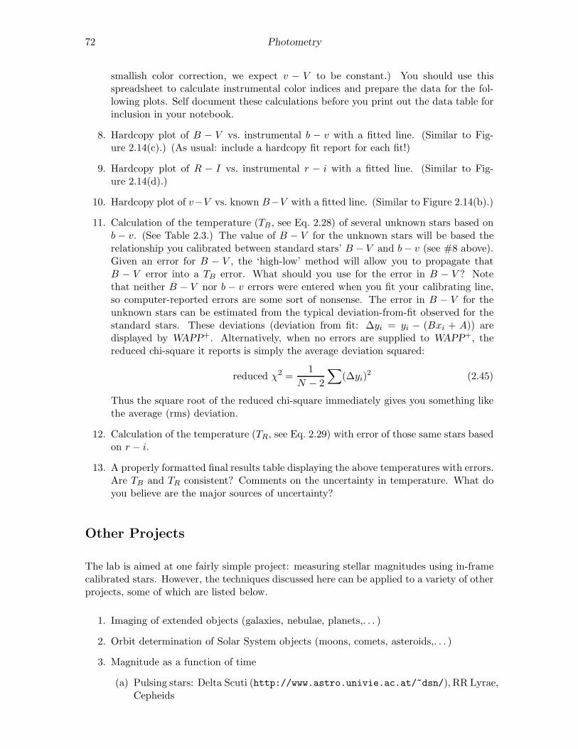
72 Photometry

smallish color correction, we expect v − V to be constant.) You should use thisspreadsheet to calculate instrumental color indices and prepare the data for the fol-lowing plots. Self document these calculations before you print out the data table forinclusion in your notebook.

8. Hardcopy plot of B − V vs. instrumental b − v with a fitted line. (Similar to Fig-ure 2.14(c).) (As usual: include a hardcopy fit report for each fit!)

9. Hardcopy plot of R − I vs. instrumental r − i with a fitted line. (Similar to Fig-ure 2.14(d).)

10. Hardcopy plot of v−V vs. known B−V with a fitted line. (Similar to Figure 2.14(b).)

11. Calculation of the temperature (TB , see Eq. 2.28) of several unknown stars based onb − v. (See Table 2.3.) The value of B − V for the unknown stars will be based therelationship you calibrated between standard stars’ B − V and b− v (see #8 above).Given an error for B − V , the ‘high-low’ method will allow you to propagate thatB − V error into a TB error. What should you use for the error in B − V ? Notethat neither B − V nor b − v errors were entered when you fit your calibrating line,so computer-reported errors are some sort of nonsense. The error in B − V for theunknown stars can be estimated from the typical deviation-from-fit observed for thestandard stars. These deviations (deviation from fit: ∆yi = yi − (Bxi + A)) aredisplayed by WAPP+. Alternatively, when no errors are supplied to WAPP+, thereduced chi-square it reports is simply the average deviation squared:

reduced χ2 =1

N − 2

∑

(∆yi)2 (2.45)

Thus the square root of the reduced chi-square immediately gives you something likethe average (rms) deviation.

12. Calculation of the temperature (TR, see Eq. 2.29) with error of those same stars basedon r − i.

13. A properly formatted final results table displaying the above temperatures with errors.Are TB and TR consistent? Comments on the uncertainty in temperature. What doyou believe are the major sources of uncertainty?

Other Projects

The lab is aimed at one fairly simple project: measuring stellar magnitudes using in-framecalibrated stars. However, the techniques discussed here can be applied to a variety of otherprojects, some of which are listed below.

1. Imaging of extended objects (galaxies, nebulae, planets,. . . )

2. Orbit determination of Solar System objects (moons, comets, asteroids,. . . )

3. Magnitude as a function of time

(a) Pulsing stars: Delta Scuti (http://www.astro.univie.ac.at/~dsn/), RR Lyrae,Cepheids

Photometry 73

(b) Cataclysmic variables (http://cba.phys.columbia.edu/)

(c) Eclipsing binaries (http://www.rollinghillsobs.org/)

(d) Novae and supernovae

(e) Rotation period of an asteroid

(f) American Association of Variable Star Observers (www.aavso.org) projects

4. Careful determination of any significant parameter of the telescope system (e.g., S/Nissues, atmospheric extinction, color corrections, tracking, . . . )

References

1. Santa Barbara Instrument Group (www.sbig.com), Operating Manual for STL-1001E,STL Operating Manual.pdf

2. Santa Barbara Instrument Group (SBIG), Users Guide for CCDOps Version 5CCDops v5.pdf

3. Meade (www.meade.com), Instruction Manual for 12” LX200LX200 Classic Manual.pdf

4. Howell, Steve B., Handbook of CCD Astronomy, Cambridge, 2000

5. Howell, Steve B., Astronomical CCD Observing and Reduction Techniques, ASP Vol.23 1992

6. Buil, Christian, CCD Astronomy, Willmann-Bell, 1991

7. Romanishin, W. An Introduction to Astronomical Photometry Using CCDs, 2006http://observatory.ou.edu

8. J. Palmer & A.C. Davenhall [starlink], The CCD Photometric Calibration Cookbook,starlink ccd.pdf

9. ed. Cox, Arthur N., Allen’s Astrophysical Quantities, AIP/Springer, 2000

10. American Association of Variable Star Observers (www.aavso.org), CCD Manualaavso ccdmanual.pdf

74 Photometry

Appendix: Available Sloan Filters: g′r′i′

The Sloan Digital Sky Survey is an ambitious project to deeply image and reduce a largefraction of the sky. The imaging is done in 5 new filters46 u′g′r′i′z′; our camera has availablethe central filters: g′r′i′. Figure 2.15 displays the characteristics of these filters.

Most any deeply exposed frame in the region imaged by SDSS will include stars withcataloged47 photometry accurate to approximately ±.03m. While this error is ∼ 10× largerthan the usual UBVRI standard stars, it is adequate for this lab. Unfortunately, manyopen clusters are not in the region imaged by SDSS (because the focus of the project isobjects beyond our Galaxy.) These Sloan magnitudes are based on the ABν system ratherthan the Vega system. Instead of the star Vega defining magnitude=0, it is intended that,for each filter, magnitude=0 corresponds to Fν = 3631 Jy. The results are not hugelydifferent from Vega-based systems: g = −.08, g − r = −0.25, r − i = −0.23 for Vega.

Various transformations of BV RI ⇐⇒ g′r′i′ for normal stars have been published48, Ireproduce a few of these results below:

B − g = 0.313(g − r) + 0.219 (2.46)

V − g = −0.565(g − r)− 0.016 (2.47)

R− r = −0.153(r − i)− 0.117 (2.48)

i− I = 0.247(R − I) + 0.329 (2.49)

r − i = 1.007(R − I)− 0.236 (2.50)

.4 .5 .6 .7 .8 .9

1.0

.8

.6

.4

.2

0

Wavelength ( m)

Tra

nsm

issi

on

g´ r´ i´

µ

Filter λ ∆λ F0

Name (µm) (µm) (W/m2 µm)

g′ .46 .13 4.71× 10−8

r′ .61 .12 2.81× 10−8

i′ .74 .12 1.87× 10−8

Figure 2.15: The characteristics of the Sloan filters: g′ (green), r′ (red), i′ (infrared) fromthe Gemini Observatory: http://www.gemini.edu and Annual Review Astronomy & As-trophysics (2005, Bessell)

46Fukugita, M., Ichikawa, T., Gunn, J. E., et al. 1996 AJ, 111, 174847http://www.sdss.org/48Jordi, K.; Grebel, E. K.; Ammon, K. A&A 460 339 (arXiv:astro-ph/0609121)

Photometry 75

.6 .8 1.0 1.2 1.4 1.6

1.4

1.2

1.0

.8

.6

.4

.2

g–r Calibration

gg–rr

g–r

(a) Calibration of the standardize color indexg − r in terms of the instrumental color indexgg− rr. See Eq. 2.44. The rms deviation fromthis calibration is about 0.03 mag.g − r = −0.29 + 1.03(gg − rr)

–.6 –.4 –.2 0

.8

.6

.4

.2

0

r–i Calibration

rr–ii

r–i

(b) Calibration of the standardize color indexr − i in terms of the instrumental color indexrr−ii. The rms deviation from this calibrationis about 0.015 mag.r − i = 0.73 + 1.14(rr − ii)

Figure 2.16: Two identical frames (taken 16-Aug-2010) of the central region of the opencluster NGC 6791 were used to calibrate the relationships between standardized color indicesand instrumental color indices . This region includes 12 standard stars (BV RIgri).

Appendix: ST-7E Camera

In June 2009 we ‘retired’ the old but fully functional SBIG ST-7E camera. I’ve dumped thespecifications for this camera in this Appendix as it is possible that it might be returnedto service. Flaws in the CCD are most evident in the bias frame49. Measurements on ourCCD shows that the difference between two bias frames shows an approximately normaldistribution (aside from the flaws) with a standard deviation ∼ 6 ADU. Also note that thesystem artificially introduces an offset of 100 into each pixel, so 2

3 of the pixels in a biasframe are expected in the range 100± 6 ADU. The ST-7 uses a thermoelectric cooler whichcan cool the CCD ∼ 30C below ambient temperature, reducing the dark currents by abouta factor of 10. The resulting dark currents are not negligible for exposures longer than afew minutes.

49Our CCD has a flaw at pixel (592, 194) which affects the entire 592 column

76 Photometry

Telescope Meade LX200aperture 12”

focal ratio f/10focal length 120”

Focal Reducer Meade f/3.3 FR/FFeffective f 50”

Filter Wheel SBIG CFW-8ACamera SBIG ST-7E ABG

pixels 765× 510image 18′ × 12′

scale 1.45”/pixel

CCD Kodak KAF-0401Epixel 9 µm× 9 µm

full-well ∼ 50, 000 e−/pixelread noise 15 e− rms

gain 2.3 e−/ADU

λ Quantum Efficiency.65 µm 60%.55 µm 50%.45 µm 40%.40 µm 30%

Table 2.4: Older CCD photometry equipment available at the SJU observatory. Note:When combined with a Celestron f/6.3 FR/FF this camera yielded 0.97”/pixel; when usedon the 10” Meade telescope without any FR/FF it yielded 1.07”/pixel.

0 5 10 15

3.E+04

2.E+04

1.E+04

0

Linearity Test

Exposure Time (s)

AD

U

0 .5 1.0 1.5

4000

3000

2000

1000

0

Linearity Test

Exposure Time (s)

AD

U

Figure 2.17: Below ∼ 30, 000 ADU (12 second exposure) the response of our CCD seems tobe linear, with saturation quite evident in the 16 second exposure. In fact, the CCD shouldnot be trusted to be linear above ∼ 25, 000 ADU.The linear fit may look good, but it is in fact not great: reduced χ2=8. Systematic errorin the shutter speed control is probably a problem for the short exposures. (Elimination ofthe two shortest exposures results in a reduced χ2=1.6.) Also note that the y intercept isnot exactly zero: with this camera zero-time exposures are designed to produce an outputof about 100 ADU.

Photometry 77

Label Name SpType b− v r − i B − V R− I TB (K) TR (K)

A BD+05 3486 A2 0.404 −0.708 0.2822 0.1826 7255 6966B GSC 00428-00981 G5 0.833 −0.387 0.8399 0.4625 5133 5015C TYC 424-517-1 K5 1.047 −0.151 1.1181 0.6683 4421 4306

Table 2.5: The instrumental color indices: b− v and r− i of the ‘unknown’ stars in IC 4665were measured using gaia and converted to standardized color indices: B − V and R − Iusing the calibration lines displayed in in Figures 2.19(c) and 2.19(d). Eq. 2.28 (TB) andEq. 2.29 (TR) were used to calculate the temperature of the stars from each color index.The two temperatures do not exactly agree; as discussed in the text systematic errors of afew percent are to be expected.

The large open cluster IC 4665 was the target for two nights during August 2005. Theresults are reported in Figures 2.19 and 2.20.

During the first night an overlapping mosaic of five frames was used to image the centralregion of the cluster. During a 2 hour period BV RI frames were taken at each pointing.(During this time the air mass to IC 4665 changed from 1.30 to 1.46, but the data showno sign of a change in the transparency of the atmosphere, so no air mass corrections wereapplied.) Dome flat-field frames (taken 12 hours earlier) were used to produce reducedframes. gaia was used to measure the instrumental magnitude of 18 standard stars andthree ‘unknown’ stars. The magnitudes were pasted into a gnumeric spreadsheet whichwas used to calculate the color indices: b − v and r − i. (Since overlapping fields wereused typically a standard star appeared in a couple of frames. When this occurred averageinstrumental color indices were used.) A calibrating line relating the standard stars’ knownB − V and the measured b− v was fit using regression in gnumeric. An identical processwas used to find the relationship between R − I and r − i. The results are displayed inFigures 2.19(c) and 2.19(d). Using these relationships and the measured instrumental colorindices, we can determine the standardized color indices of any star in the imaged region.As shown in Table 2.5, Eq. 2.28 or Eq. 2.29 can then be used to find the temperature ofeach ‘unknown’ star.

During the second night six (generally not overlapping) frames were selected with the aimof capturing a diverse (hot and cool) set of standard stars. The data collected during thisnight did show a change in the transparency of the atmosphere (there was a larger variationin air mass: 1.32 to 1.63; see Figure 2.20(a)), so air mass corrections were applied.

78 Photometry

200 400 800 2000 4000 8000

.999

.99

.9

.5

.1

.01

.001

Distribution of Pixel Dark Current

ADU

Per

cent

ile

–10˚ C

+10˚ C

(a) The distribution of pixel dark current at+10C and −10C. All but a few of the pixelshave a (log)normal distribution of dark current.A few percent of the pixels show much largerdark current: these are the ‘hot’ pixels. Notethat both classes of pixels respond to temper-ature: lowering the temperature reduces everypixel’s dark current.

0 10 20 30 40

4000

2000

800

400

200

Along a Row: Dark Current

pixel

AD

U

(b) Part of a row of pixels is displayed at threetemperatures: • = +10C, = 0C, H =−10C. Isolated hot pixels are randomly sprin-kled throughout the image (here at columns 12and 20). The data here and in (a) are from 15minute dark frames.

0 5 10 15

4000

3000

2000

1000

Temperature ‘cools’ Hot Pixels

Time (min)

AD

U

0˚ C

+10˚ C

–10˚ C

(c) Dark current produces ever larger storedcharge in a pixel; of course reducing the tem-perature reduces the dark current.

0 5 10 15

150

140

130

120

110

100

Normal Pixels at –10˚ C

Time (min)

AD

U

(d) While it is more evident in this low countdata, there is always deviation in counts. Whilewe can subtract the average dark charge, devi-ations from the average produce ‘noise’ in ourimages. Reducing the temperature reduces thisnoise.

Figure 2.18: Dark frames are ‘exposures’ with the shutter closed. The source of thesecounts is not starlight, rather a thermally induced current allows charge to accumulate ineach pixel. This ‘dark current’ can be exceptionally large in ‘hot pixels’.

Photometry 79

(a) This Digitized Sky Survey image shows thecentral ∼ 50′ × 25′ region of the open clusterIC 4665. The standard stars of J.W. Menziesand F. Marang (MNRAS, 282, 313–316 (1996))are labeled along with three ‘unknown’ stars:A, B, C.

.2 .4 .6 .8 1.0 1.2 1.4 1.6

28.26

28.24

28.22

28.20

28.18

28.16

28.14

v–V Calibration

b–v

v–V

(b) There is little evidence for a significantcolor correction in this data set. See Eq. 2.42.

.2 .4 .6 .8 1.0 1.2 1.4 1.6

1.5

1.0

.5

0

B–V Calibration

b–v

B–V

(c) Calibration of the standardize color indexB−V in terms of the instrumental color indexb− v. See Eq. 2.44.

–1.0 –.8 –.6 –.4 –.2 0 .2

1.0

.8

.6

.4

.2

0

R–I Calibration

r–i

R–I

(d) Calibration of the standardize color indexR − I in terms of the instrumental color indexr − i.

Figure 2.19: An overlapping mosaic of five frames was used to image the central region of theopen cluster IC 4665. This region includes 18 standard stars which were used to calibratethe relationships between standardized color indices and instrumental color indices. Usingthese relationships and the measured instrumental color indices, we can determine thestandardized color indices of any star in the imaged region.

80 Photometry

1.35 1.40 1.45 1.50 1.55 1.60

31.46

31.44

31.42

31.40

31.38

31.36

Air Mass Corrections

Air Mass

<b–

B>

or

<i–

I>

(a) Short wavelengths are more affected byatmospheric absorption than long; the aboveshows the effect on B magnitudes (filledsquares) and I magnitudes (open circles). They axis displays the difference between instru-mental and standardized magnitudes averagedover all the blue stars in the frame.

.6 .8 1.0 1.2 1.4 1.6 1.8

30.96

30.94

30.92

30.90

30.88

30.86

Color Correction

b–v

v–V

(b) Color correction is evident in this data set,but both air mass and color correction shouldbe applied to this data. This full result was:v − V = 30.611 + 0.179 sec z + 0.048(b − v).The rms variation from this line was less than0.02 mag.

.6 .8 1.0 1.2 1.4 1.6 1.8

1.5

1.0

.5

0

B–V Color Calibration

b–v

B–V

(c) Calibration of the standardize color indexB−V in terms of the instrumental color indexb− v.B − V = −0.67 + 1.29(b − v)

–.8 –.6 –.4 –.2 0 .2

.8

.6

.4

.2

0

R–I Color Calibration

r–i

R–I

(d) Calibration of the standardize color indexR − I in terms of the instrumental color indexr − i.R − I = 0.80 + 0.86(r − i)

Figure 2.20: Six frames were used to image 22 standard stars in the open cluster IC 4665.The selected stars have a wide variation in color in order to to achieve robust color cali-brations. During the 2+ hours of data collection the air mass increased from 1.32 to 1.63and the resulting increase in atmospheric absorption increased (dimmed) B,V,R, and Imagnitudes in proportion to the air mass (see Figure 2.20(a)).

3: Electrical Measurements Review

Pre-Lab: Read and understand this chapter before coming to lab!Complete the following problems: 1a, 3–9, 11, 15–21Record the results in your notebook.

Lab: See page 98. Work as individuals!Lab in room PE116. Begin: 10 February; Due: 21 February

Reference: Horowitz & Hill, The Art of ElectronicsChapter 1 & Appendix ADiefenderfer & Holton, Principles of Electronic InstrumentationChapter 6Paul Scherz, Practical Electronics for Inventors, 2nd edition

Purpose

This review aims to re-familiarize you with the electronic instrumentation you used inPhysics 200 lab: components like resistors and capacitors, measuring devices like digitalmultimeters and oscilloscopes, and electrical sources like function generators and d.c. powersupplies. In addition the usual schematic symbols for these devices are presented.

Components

In Physics 200 you learned about three passive, linear components: resistors (R), capacitors(a.k.a., condensers, C) and inductors (a.k.a., chokes or coils, L). These devices are calledpassive because they require no outside power source to operate (and thus circuits involvingjust these components cannot amplify: at best power in = power out). These devices arecalled linear because the current through these devices is linearly proportional to the voltageacross them1:

I =1

ZV (3.1)

1Unless otherwise stated, you should always assume that “voltage” and “current” refers to the root-mean-square (rms) value of that quantity. That is what meters always report. Of course, this equation would alsoapply to peak or peak-to-peak values as long as they are consistently used.

81

82 Electrical Measurements Review

R

2πfCXC =

1

C L

XL = 2πfL

ground diodeanode

cathode

Figure 3.1: The schematic symbols for common components including resistors (R), capac-itors (C), and inductors (L). For these three “linear” devices there is a linear relationshipbetween the current through the device (I) and the voltage across the device (V ). Forresistors, the resistance, R = V/I is constant. For capacitors and inductors the reactanceX = V/I depends on frequency (f) as shown above. The two symbols for ground (zerovolts) are, respectfully, chassis and earth ground.

The impedance Z (unit: Ω) determines the proportionality constant. Large impedances(think MΩ) mean small currents (think µA) flow from moderate driving voltages. Smallimpedances (think 1 Ω) mean large currents (1 A) flow from moderate driving voltages.Impedance2 is an inclusive term: for resistors the impedance is called resistance; for in-ductors and capacitors the impedance is called reactance. Inductors and capacitors areuseful only in circuits with changing voltages and currents. (Note: changing voltage and/orcurrent = alternating current = a.c.; unchanging current/voltage = direct current = d.c..)The reactance (or impedance) of inductors and capacitors depends on the frequency f ofthe current. A capacitor’s impedance is inversely proportional to frequency, so it impedeslow frequency signals and passes high frequency signals. An inductor’s impedance is pro-portional to frequency, so it impedes high frequency currents but passes low frequencycurrents. Recall that current and voltage do not rise and fall simultaneously in capacitorsand inductors as they do in resistors. In the inductors the voltage peaks before the currentpeaks (voltage leads current, ELI). In capacitors the current peaks before the voltage peaks(current leads voltage, ICE).

Diodes are non-linear passive devices. Positive voltages on one terminal (the anode) resultsin large current flows; positive voltages on the other terminal (the cathode) results inessentially no current flow. Thus the defining characteristic of diodes is easy current flow inonly one direction. The arrow on the schematic symbol for a diode shows the easy directionfor current flow. On a diode component a white line often marks which terminal allowseasy outward flow.

Light Emitting Diodes (LED) are specialized diodes in which part of the electrical power(I∆V ) is dissipated as light rather than heat. The color of the emitted light (from IR toUV) depends on the material and ∆V .

2Impedance is often distinguished as being a complex quantity (as in Z = a + bi, where i =√−1 and

a, b ∈ R). Resistors then have real impedances whereas Z is purely imaginary for inductors and capacitors.This advanced approach is followed in Physics 338. In Physics 200 this reality is hidden behind ‘phasers’.

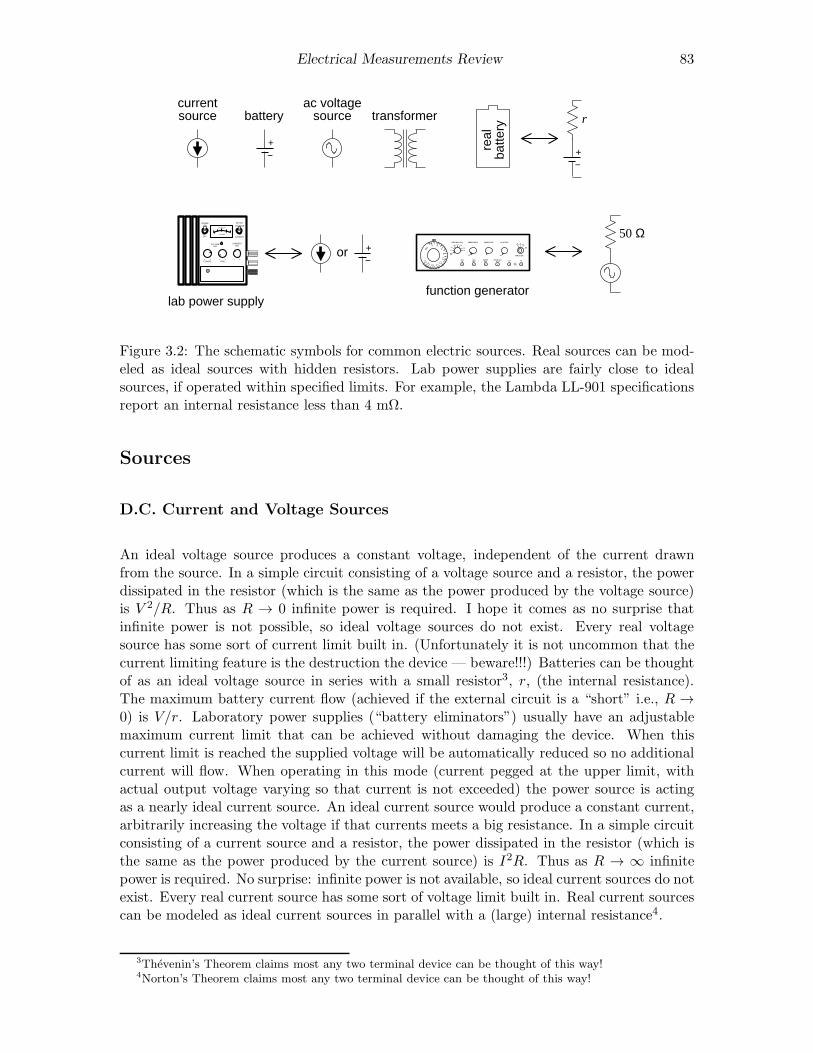
Electrical Measurements Review 83

+−

transformerac voltage

sourcecurrent source battery

POWERON

OFF

VOLTAGE

CURRENT

METER

COARSE FINE

VOLTAGEADJ

CURRENTADJ

DC AMPS

DC VOLTS

+−

or

lab power supply

real

batte

ry

+−

r

PWROFF

× 1

× 10

× 100× 1K

× 10K

× 100K

× 1M

FREQ MULT (Hz) SWEEP WIDTH SWEEP RATE DC OFFSET

HILOPULSE OUT(TTL)

SWEEPOUT

GCVOUT

VCGIN

OFF OFF

50 ΩOUT

DC

AMPLITUDE

.2 .4

.6.8

1.0

1.21.41.61.8

2.0

.002

function generator

50 Ω

Figure 3.2: The schematic symbols for common electric sources. Real sources can be mod-eled as ideal sources with hidden resistors. Lab power supplies are fairly close to idealsources, if operated within specified limits. For example, the Lambda LL-901 specificationsreport an internal resistance less than 4 mΩ.

Sources

D.C. Current and Voltage Sources

An ideal voltage source produces a constant voltage, independent of the current drawnfrom the source. In a simple circuit consisting of a voltage source and a resistor, the powerdissipated in the resistor (which is the same as the power produced by the voltage source)is V 2/R. Thus as R → 0 infinite power is required. I hope it comes as no surprise thatinfinite power is not possible, so ideal voltage sources do not exist. Every real voltagesource has some sort of current limit built in. (Unfortunately it is not uncommon that thecurrent limiting feature is the destruction the device — beware!!!) Batteries can be thoughtof as an ideal voltage source in series with a small resistor3, r, (the internal resistance).The maximum battery current flow (achieved if the external circuit is a “short” i.e., R →0) is V/r. Laboratory power supplies (“battery eliminators”) usually have an adjustablemaximum current limit that can be achieved without damaging the device. When thiscurrent limit is reached the supplied voltage will be automatically reduced so no additionalcurrent will flow. When operating in this mode (current pegged at the upper limit, withactual output voltage varying so that current is not exceeded) the power source is actingas a nearly ideal current source. An ideal current source would produce a constant current,arbitrarily increasing the voltage if that currents meets a big resistance. In a simple circuitconsisting of a current source and a resistor, the power dissipated in the resistor (which isthe same as the power produced by the current source) is I2R. Thus as R → ∞ infinitepower is required. No surprise: infinite power is not available, so ideal current sources do notexist. Every real current source has some sort of voltage limit built in. Real current sourcescan be modeled as ideal current sources in parallel with a (large) internal resistance4.

3Thevenin’s Theorem claims most any two terminal device can be thought of this way!4Norton’s Theorem claims most any two terminal device can be thought of this way!

84 Electrical Measurements Review

A.C. Voltage Sources

A function generator is a common source of a.c. signals. A function generator can producea variety of wave shapes (sinusoidal, square, triangle, . . . ) at a range of frequencies, andcan even ‘sweep’ the frequency (i.e., vary the frequency through a specified range during aspecified period). Usually the signals are balanced (i.e., produces as much positive voltageas negative), but a d.c. offset can be added to the signal, for example, producing a voltageof the form

A cos(2πft) +B (3.2)

(In this case the d.c. offset would be B, the amplitude would be A, and the peak-to-peakvoltage would be 2A.) Most function generators are designed to have an internal resistanceof 50 Ω and maximum voltage amplitude of around 10 V. Generally they have a poweroutput of at most a few watts.

Certainly the most common a.c. source is the wall receptacle: 120 V at a frequency of60 Hz. Transformers can be used to reduce this voltage to less dangerous levels for lab use.A ‘variac’ (a variable transformer) allows you to continuously vary the voltage: 0–120 V.Relatively large power (> 100 W) and current (> 1 A) can be obtained in this way. Ofcourse the frequency is not changed by a transformer; it would remain 60 Hz.

Electrical Measurement

Digital Multimeter (DMM)

The most common measurement device is the digital multimeter (DMM). Feel free to callthese devices ‘voltmeters’, but in fact they can measure much more than just volts. Forexample, the Keithley 169 is fairly generic, measuring volts (a.c. and d.c.), amps (a.c. andd.c.), and ohms. The hand-held Metex M-3800 measures the above and adds transistorhFE and diode test. The bench-top DM-441B measures all of the above and frequency too.The ease of switching measurement options should not blind you to the fact that thesemeasurement options put the DMM into radically different modes. If, for example, theDMM is properly hooked up to measure voltage and — without changing anything else —you switch the DMM to measure amps, most likely something will be destroyed: either theDMM or the device it is connected to. Please be careful!

Recall that voltage (or more properly potential difference) is a measurement of the electrical‘push’ applied to an electron as it moves through a section of the circuit. It is analogousto water pressure in that the difference in the quantity determines the driving force. (Nopressure difference; no net force.) Note that the presence of big ‘push’, in no way guaranteesthat there will be a large resulting flow (current). A large resistance (or for a.c. circuits,impedance) can restrict the flow even in the presence of a big push. In fact, large currentflows are often driven by very small voltage differences as a very fat (small resistance) wireis provided for the flow. Wires work by having very small resistance; an ideal wire has zeroresistance, and hence nearly zero voltage difference between its two ends.

Electrical Measurements Review 85

A

an ammeter acts like a short circuit

V

a voltmeter acts like a open circuit

Figure 3.3: The schematic symbols for basic meters. An ammeter must substitute for anexisting wire to work properly, whereas a voltmeter can be attached most anywhere.

A voltmeter measures the potential difference across or between the two selected points. Agood voltmeter is designed to draw only a small current so it must be equivalent to a largeresistance. Modern DDMs typically have input impedances greater than 1 MΩ. Voltmeterswith even larger resistance (TΩ) are called electrometers. An ideal voltmeter would drawno current; it would be equivalent to an ‘open circuit’. (An open circuit [R → ∞] is theopposite of ‘short circuit’ [R → 0] which is obtained if the two points are connected by anideal wire.) Since voltmeters draw only a small current, they should not affect the circuitbeing measured. This makes the voltmeter an excellent diagnostic tool.

Voltmeters always measure the voltage difference between the two probes (e.g., to measurethe ‘voltage across’ a device place probes at opposite ends of the device), but occasionallyyou are asked to measure the voltage at a point. Those words imply that the black (a.k.a.common) probe is to be placed at ground. (In fact you’ll soon learn that oscilloscopes aredesigned as one-probe-at-ground voltmeters.)

Measurement of the current flow through a wire, necessarily requires modification of thecircuit. The flow normally going through the wire must be redirected so it goes through theammeter. This requires breaking the path that the current normally uses, i.e., cutting thewire and letting the ammeter bridge the two now disconnected ends. (With luck, the wiremay not need to be literately cut, perhaps just disconnected at one end.) Because currentmeasurements require this modification of the circuit under study, one generally tries toavoid current measurements, and instead substitute a voltage measurement across a devicethrough which the current is flowing. Knowledge of the impedance of the device will allowyou to calculate the current from the voltage. Because an ammeter substitutes for a wire,it should have a very small resistance. An ideal ammeter would have zero resistance, i.e.,be a short circuit between its two leads. (Note that this is the opposite of a voltmeter,which ideally has an infinite resistance between its two leads.) Real ammeters require asmall voltage drop (typically a fraction of a volt for a full scale reading) to operate. Thissmall ∆V is called the voltage burden.

I say again: converting a DMM from voltmeter to ammeter makes a drastic change fromopen circuit to short circuit. Making such a switch in a DMM connected to a circuit usuallyresults in damaging something. Poking around in a circuit with a voltmeter is unlikely tocause damage, because the voltmeter acts like a huge resistor (not that different from theair itself). Poking around in a circuit with an ammeter is quite likely to cause damage, asit is linking two points with a wire, i.e., adding short circuits between points in the circuit.

A DMM measures resistance by forcing a current through the leads and, at the same time,measuring the potential difference between the leads. The resistance can then be calculatedby the DMM from R = V/I. Note that since a DMM in resistance mode is sending a

86 Electrical Measurements Review

current through its leads (‘sourcing current’) and assuming that this current is the onlycurrent flowing through the device, you cannot measure the resistance of a powered device.Furthermore, you can almost never use the DMM to measure the resistance of a deviceattached to an existing circuit because the current injected by the DMM may end loopingback through the circuit rather than through the device. (In addition injecting current intoa circuit at random places may damage some components in the circuit.) Thus to measurethe resistance of something, you almost always have to disconnect at least one end of itfrom its circuit.

Lab Reminder: For accurate measurement you must use the appropriate scale: thesmallest possible without producing an overscale. DMM’s may report an overscale conditionby a flashing display or a nonsense display like: . Similarly, for significant DMMmeasurements you should record in your notebook every digit displayed by the DMM.

A.C. DMM Measurements

Some special considerations are needed when using a DMM to measure a.c. currents orvoltages. First, DMMs give accurate readings only for frequencies in a limited range. DMMsfail at low frequencies because DMMs report several readings per second and, in order tobe properly measured, the signal needs to complete at least one cycle per reading frame.Thus f > 20 Hz or so for accurate readings. At the high frequencies, the input capacitance(∼ 100 pF) of the DMM tends to short out the measurement (recall the impedance of acapacitor at high frequency is small). No SJU DMM operates accurately above 0.3 MHz;some DMMs have trouble above 1 kHz. The DMM’s manual, of course, reports thesespecifications.

Recall that a.c. signals are time-variable signals . . . there is no steady voltage to report as“the” voltage. The solution is to report root-mean-square (‘rms’) quantities. (The squareroot of the average of the square of the voltage.) Since this is a complex thing to calculate,most cheap DMMs assume that the signal is sinusoidal so that there is a relationship betweenthe rms value and the peak value:

Vrms = Vpeak/√2 (3.3)

These cheap DMMs find the peak voltage, divide it by√2 and report the result as if it

were an rms voltage. This of course means the meter reports faulty values if non-sinusoidalsignals are applied. “True rms” meters properly calculate the rms quantities.

Oscilloscope

Generally speaking DMMs work in the ‘audio’ frequency range: 20 Hz – 20 kHz. ‘Radiofrequency’ (rf, say frequencies above 1 MHz) require an alternative measuring device: theoscilloscope (a.k.a., o’scope or scope). Unlike the DMM, the oscilloscope usually measuresvoltage (not current). Also unlike the DMM, the scope effectively has only one lead: the‘black’ lead of the scope is internally connected to ground; the voltage on the ‘red’ lead isdisplayed on the screen. (Note: with a DMM you can directly measure the 1 V potentialdifference between two terminals at 100 V and 101 V. You cannot do this with a scope—its‘black’ lead is internally connected to ground so if you connect it’s ‘black’ lead to the 100 V

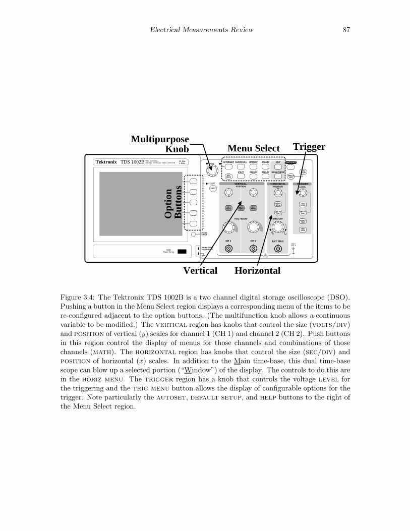
Electrical Measurements Review 87

REFMENU

SET TOZERO

SET TO50%

TRIGMENU

HORIZMENU

TRIGVIEW

FORCETRIG

UTILITY CURSOR

AUTORANGE SAVE/RECALL MEASURE ACQUIRE

DISPLAY DEFAULT SETUP

HELP

PRINT

SAVE

EXT TRIGCH 2CH 1

SEC/DIV

HORIZONTALPOSITIONPOSITION

VERTICAL

RUN/STOP

SINGLESEQ

AUTOSET

TRIGGERLEVEL

VOLTS/DIV

Tektronix TDS 1002BTWO CHANNELDIGITAL STORAGE OSCILLOSCOPE

60 MHz1 GS/s

PROBECHECK

PROBE COMP~5V@1kHzUSB

Flash Drive

300 VCAT II

!

CH 1MENU

MATHMENU

CH 2MENU

Horizontal

Menu Select

Opt

ion

But

tons

MultipurposeKnob Trigger

Vertical

Figure 3.4: The Tektronix TDS 1002B is a two channel digital storage oscilloscope (DSO).Pushing a button in the Menu Select region displays a corresponding menu of the items to bere-configured adjacent to the option buttons. (The multifunction knob allows a continuousvariable to be modified.) The vertical region has knobs that control the size (volts/div)and position of vertical (y) scales for channel 1 (CH 1) and channel 2 (CH 2). Push buttonsin this region control the display of menus for those channels and combinations of thosechannels (math). The horizontal region has knobs that control the size (sec/div) andposition of horizontal (x) scales. In addition to the Main time-base, this dual time-basescope can blow up a selected portion (“Window”) of the display. The controls to do this arein the horiz menu. The trigger region has a knob that controls the voltage level forthe triggering and the trig menu button allows the display of configurable options for thetrigger. Note particularly the autoset, default setup, and help buttons to the right ofthe Menu Select region.

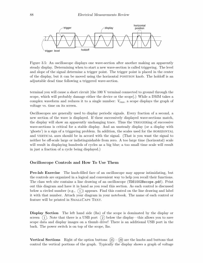
88 Electrical Measurements Review

trigger

holdofftrigger level

displayhorizontalposition

Figure 3.5: An oscilloscope displays one wave-section after another making an apparentlysteady display. Determining when to start a new wave-section is called triggering. The leveland slope of the signal determine a trigger point. The trigger point is placed in the centerof the display, but it can be moved using the horizontal position knob. The holdoff is anadjustable dead time following a triggered wave-section.

terminal you will cause a short circuit [the 100 V terminal connected to ground through thescope, which will probably damage either the device or the scope].) While a DMM takes acomplex waveform and reduces it to a single number: Vrms, a scope displays the graph ofvoltage vs. time on its screen.

Oscilloscopes are generally used to display periodic signals. Every fraction of a second, anew section of the wave is displayed. If these successively displayed wave-sections match,the display will show an apparently unchanging trace. Thus the triggering of successivewave-sections is critical for a stable display. And an unsteady display (or a display with‘ghosts’) is a sign of a triggering problem. In addition, the scales used for the horizontaland vertical axes should be in accord with the signal. (That is you want the signal toneither be off-scale large or indistinguishable from zero. A too large time (horizontal) scalewill result in displaying hundreds of cycles as a big blur; a too small time scale will resultin just a fraction of a cycle being displayed.)

Oscilloscope Controls and How To Use Them

Pre-lab Exercise The knob-filled face of an oscilloscope may appear intimidating, butthe controls are organized in a logical and convenient way to help you recall their functions.The class web site contains a line drawing of an oscilloscope (TDS1002Bscope.pdf). Printout this diagram and have it in hand as you read this section. As each control is discussedbelow a circled number (e.g., 1m) appears. Find this control on the line drawing and labelit with that number. Attach your diagram in your notebook. The name of each control orfeature will be printed in SmallCaps Text.

Display Section The left hand side (lhs) of the scope is dominated by the display orscreen 1m. Note that there is a USB port 2mbelow the display—this allows you to savescope data and display images on a thumb drive! There is an additional USB port in theback. The power switch is on top of the scope, lhs.

Vertical Sections Right of the option buttons 25m– 29mare the knobs and buttons thatcontrol the vertical portions of the graph. Typically the display shows a graph of voltage

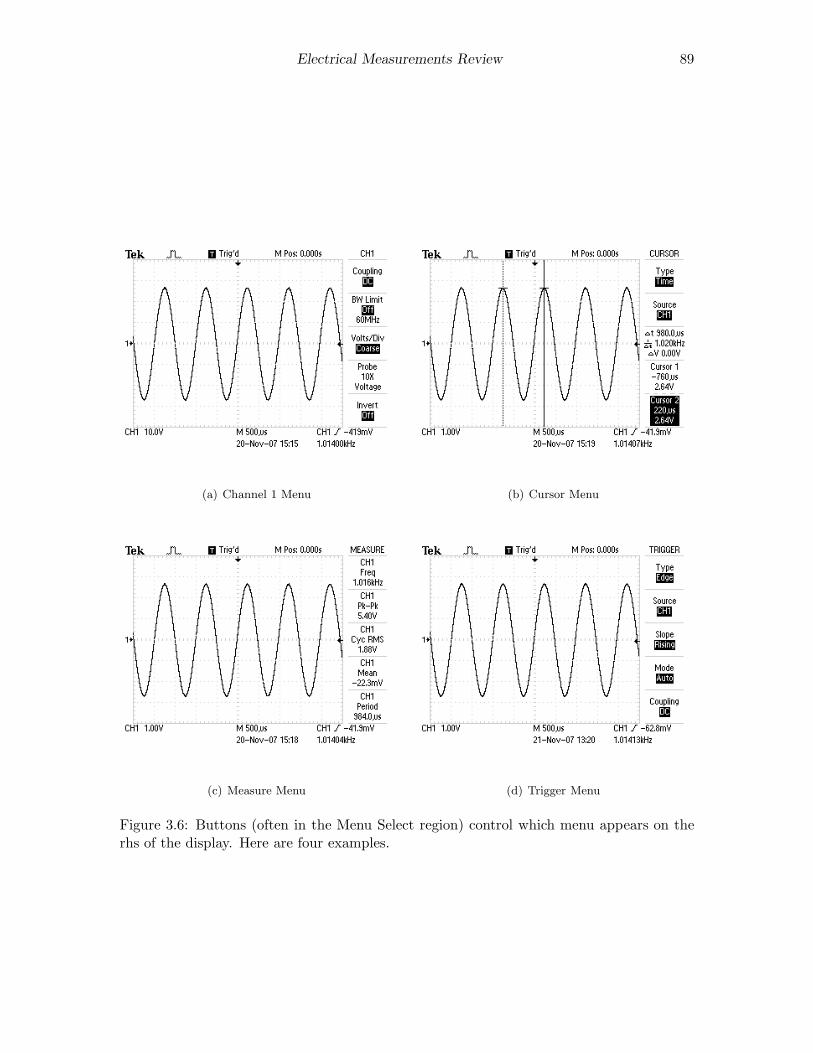
Electrical Measurements Review 89

(a) Channel 1 Menu (b) Cursor Menu

(c) Measure Menu (d) Trigger Menu

Figure 3.6: Buttons (often in the Menu Select region) control which menu appears on therhs of the display. Here are four examples.

90 Electrical Measurements Review

(y or vertical) vs. time (x or horizontal). This scope has two BNC5 inputs so the verticalsection is divided into two sections with identical controls for each input. The inputs arecalled channel 1 (CH 1) 5mand channel 2 (CH 2) 10m. The scale factor for each input isdetermined by the corresponding volts/div knob 6m& 11m; the vertical location of zerovolts on the screen is determined by the corresponding position knobs 8m& 13m. Notethat the scale factors and the zero location for the channel traces are independently set.Therefore the graph axes can not show values in physical units (volts), rather the graph isdisplayed on a 8× 10 grid with units called divisions. (Note that a division is about a cm.)

The volts/div (or sensitivity) knobs are similar to the range switch on a multimeter. Todisplay a 2 volt signal, set the volts/div knob to 0.5 volts/div. A trace 4 div high willthen be obtained, since 4 div × 0.5 V/div = 2 V. The current settings of these sensitivityknobs is displayed in the lower lhs of the display. You should always adjust the sensitivityso that the signal displayed is at least 3 div peak-to-peak.

The traces from the two channels look identical on the screen; the symbols 1- and 2- onthe lhs of the display show the position of zero volts for each trace. If you are unsure whichtrace is which, moving a position knob will immediately identify the corresponding trace.

The ch 1 and ch 2 menu buttons 7m& 12mproduce menus controlling how the corre-sponding input is modified and displayed. In addition pushing these menu buttons togglesthe display/non-display of the corresponding signal.

The top menu item in ch 1 and ch 2 menus, is Coupling, with options: DC, AC, Ground.These options control how the signal supplied to the BNC is connected (coupled) to thescope’s voltage measuring circuits. The Ground option means the scope ignores the input andinstead the display will graph a horizontal line at zero volts (ground) — this allows you toprecisely locate and position the zero volt reference line for that channel on the grid. WhenAC is selected a capacitor is connected between the inputted signal and scope’s electronics.This capacitor prevents any d.c. offset voltage from entering the scope’s circuits. Thus anyd.c. offset will be subtracted from the signal and the display will show the remaining signaloscillating around a mean of zero volts. The usual selection for Coupling is DC, which meansthe signal is displayed unmodified.

Proper Practice: Use CouplingDC almost always. Exceptional circumstances like a d.c.offset larger than an interesting a.c. signal (i.e., B ≫ A in Eq. 3.2) or a requirement tomeasure an rms voltage in the usual way, i.e., with any d.c. offset removed, may forceoccasional, brief uses of CouplingAC, but don’t forget to switch back to CouplingDCASAP.

In between the ch 1 and ch 2 menu buttons, find the math menu 9mbutton. which isused to display combinations of CH 1 and CH 2 (+,−,×) and Fourier transforms (FFT)of either signal.

5According to Wiki, this denotes “bayonet Neill-Concelman” connector. This coaxial cable connector isvery commonly used when signals below 1 GHz are being transmitted. You can also use Wiki to learn aboutbanana connectors and alligator clips (a.k.a. crocodile clips).

Electrical Measurements Review 91

Probe The second item from the bottom in the ch 1 and ch 2menus is Probe. “Probe” is the name for the device/wire that con-nects the scope to the signal source. In this course most often yourprobe will be nothing more complex than a wire, so the choice shouldbe 1X Voltage. Note that this is not the factory default choice (whichis 10X Voltage). So one of the first things you should do on turningon a scope, is check that the the probe actually attached to the scopematches what the scope thinks is attached to the scope. (If there isa mis-match, all scope voltage measurements will be wrong.) Thereis a probe check button 3mon the scope to help you establish theattenuation of an unlabeled probe, but usually probes are labeledand it is faster just to immediately set the probe type yourself in thecorresponding channel menu. Note: most probes used in this classhave a switch to select either 10× or 1× attenuation. All SJU probesare voltage probes.

10X1X

Input

Ground

1× or 10×Switch

Note: A probe is a scope-only accessory: it should not be attached to any other device.(While a simple wire can act as a scope probe, a scope probe is in general more than asimple wire and therefore should not substitute for a simple wire.)

FYI: The name “10×” on a probe is quite confusing: “÷10” would be a better name asthe voltage that reaches the scope has been reduced by a factor of 10. Why reduce a signalbefore measuring it? Because it reduces the probe’s impact on the circuit it is connected to.A 10× probe has a larger impedance (smaller capacitance and larger resistance) than a 1×probe and hence affects the circuit less. This is particularly important for high frequencymeasurements (which are not the focus of this class).

Horizontal Section In the center-right of the scope face, find the horizontal section.Just as in the vertical sections, there are knobs that control the horizontal scale (sec/div

15m) and horizontal position 18m. In a single time-base scope, all the input channels mustbe displayed with the same horizontal scale (unlike the vertical scale). In this dual timebase scope, a portion of the display can be expanded in a Window. The window controls arefound in the horiz menu 17m. When using the window feature the Main sec/div setting islabeled M and the Window sec/div setting is labeled W.

Trigger Section As you might guess, the process of determining when to trigger anddisplay the next wave-section is the most complex part of a scope. Luckily most oftenthe default settings will work OK. Generally you will want to trigger when the wave hasreached a particular level 23m. But which wave? The trig menu 22mallows you toset the Source: CH1, CH2, Ext (the signal connected to the ext trig BNC 14min thehorizontal section), Ext/5 (the same signal, but first attenuated by a factor of 5—useful forlarger triggering signals), or AC Line (which uses the 60 Hz, 120 V receptacle power lineas the triggering signal—useful for circuits that work synchronously with the line voltage).Just as in the vertical section, the Coupling of this source to the triggering electronics canoccur in a variety of ways: subtract the dc offset (AC), filter out (attenuate or remove) highfrequency (HF Reject, “high” means > 80 kHz), filter out low frequency (LF Reject, “low”means < 300 kHz), use hysteresis to reduce the effects of noise (Noise Reject), or directly

92 Electrical Measurements Review

connected (DC). Note: triggering with CouplingAC is a common choice as then a level ofzero is sure to match the wave at some point. Similarly Noise Reject is not an uncommonchoice. The above options go with TypeEdge. There are additional sophisticated anduseful triggering modes for TypePulse and TypeVideo.

Measure Menu The measure menu 36mallows up to five measurements to be con-tinuously updated and displayed. Push on one of the option buttons and a new menu isdisplayed allowing you to set the Source: CH1, CH2, MATH, and the Type: Freq, Period,Mean (voltage), Pk-Pk (peak-to-peak, i.e., the full range of voltage from the lowest valley tothe highest peak), Cyc RMS (the root-mean-square voltage of the first complete cycle), Min(minimum voltage), Max (maximum voltage), Rise Time, Fall Time (10% to 90% transitions),Pos(itive) Width, Neg(itive) Width (using the 50% level).

Warning: Unlike a DMM on AC, the option Cyc RMS does not subtract the d.c. offsetbefore calculating rms voltage. You can assure yourself of a DMM-like rms result only ifthe channel is switched to CouplingAC.

If a measurement is displayed with a question mark, try switching scales. (Generally thescope wants signals that are several divisions high and complete at least one—but not toomany—cycles in the display.)

Cursor Menu The cursor menu 37menables a pair of TypeAmplitude or TypeTimemeasuring lines. With Amplitude cursors, a pair of horizontal lines (“cursors”) appears.Hitting the appropriate option button allows the multifunction knob to move each cursorup or down to the required place. The voltage for each cursor is displayed along with thedifference (∆V ). With Time cursors, a pair of vertical lines appears. Hitting the appropriateoption button allows the multifunction knob to move each line (cursor) right or left to therequired place. The voltage and time for each cursor is displayed along with the differences(∆t, ∆V ), and frequency 1/∆t.

Display Values The bottom of the display is used to report key numerical values likescale settings. A typical example:

CH1 500mV CH2 2.00V M 1.00ms CH1 0.00V23-Nov-07 13:03 1.01407kHz

The first two numbers of the first line are the volts/div for channels CH1 and CH2, Mrefers to the main time-base of 1 ms/div, and the final sequence reports that positive edgetriggering at a level of 0.00 V is being used with channel 1 as the source. The second lineshows the date/time and the frequency of the triggering signal.

Run/Stop In normal operation, the scope is constantly updating the display. It is pos-sible to freeze the display (i.e., take a snapshot of the voltage vs. time graph) using therun/stop 44mor single seq 43mbuttons.

Electrical Measurements Review 93

Hit Me First The scope remembers option settings between uses. Thus unless you are thesole user of the scope it is wise to set it to a well defined initial state before proceeding. Thedefault setup 41machieves this goal (but it sets the Probe10X Voltage, in the channelmenus—which is not usually desired in this class). Similarly the autoset 42mbutton willattempt to make rational choices for scale factors, etc. given the signals connected to thescope. If you want you can save commonly used setups using the save/recall 34mmenubutton.

Problems

1. (a) A 1.5 V battery can be modeled as an ideal 1.5 V voltage source in series with a1 Ω resistor. If this battery is connected to a 10 Ω resistor (see below left), whatvoltage is actually across the 10 Ω resistor?

(b) A 1 mA current source can be modeled as an ideal 1 mA current source in parallelwith a 1 MΩ resistor. If this source is connected to a 10 kΩ resistor (see belowright), how much current actually flows through the 10 kΩ resistor.?

+−

1 Ω

1.5 V

1.5

V b

atte

ry

10 Ω 1 M

Ω

1 m

A

power supplycurrent source

10 kΩ

2. (a) A voltage source produces a voltage V when its terminals are disconnected (opencircuit). When a device that draws a current I is connected across its terminals,the voltage decreases to V −∆V . What is the internal resistance?

(b) A current source produces a current of I when a wire connects the terminals.When a device is instead connected to the terminals the current drops to I −∆Iand the voltage across the terminals is V . What is the internal resistance?

3. The manual for a stereo amplifier warns that it can be damaged if its “outputs aretoo heavily loaded”. What sort of resistor would constitute a “heavy load”: (A)R = 1 MΩ or (B) R = 1 Ω? Explain!

4. (a) A current of 3 mA flows into a circuit consisting of 3 resistors, and 10 mAflows out (see below left). Report the readings on the three voltmeters. Draw aschematic diagram showing which lead on each voltmeter is the ‘red’ lead.

(b) An unknown device is connected in a circuit with a 9 V battery and a 15 kΩresistor (see below right). The ammeter reads 0.5 mA. What does the voltmeterread?

5.6 kΩ

2.7 kΩ1.8 kΩ

3 mA

10 mAV2

V1

V3

+− 9 V

15 kΩ

devi

ce V

A

?? mA

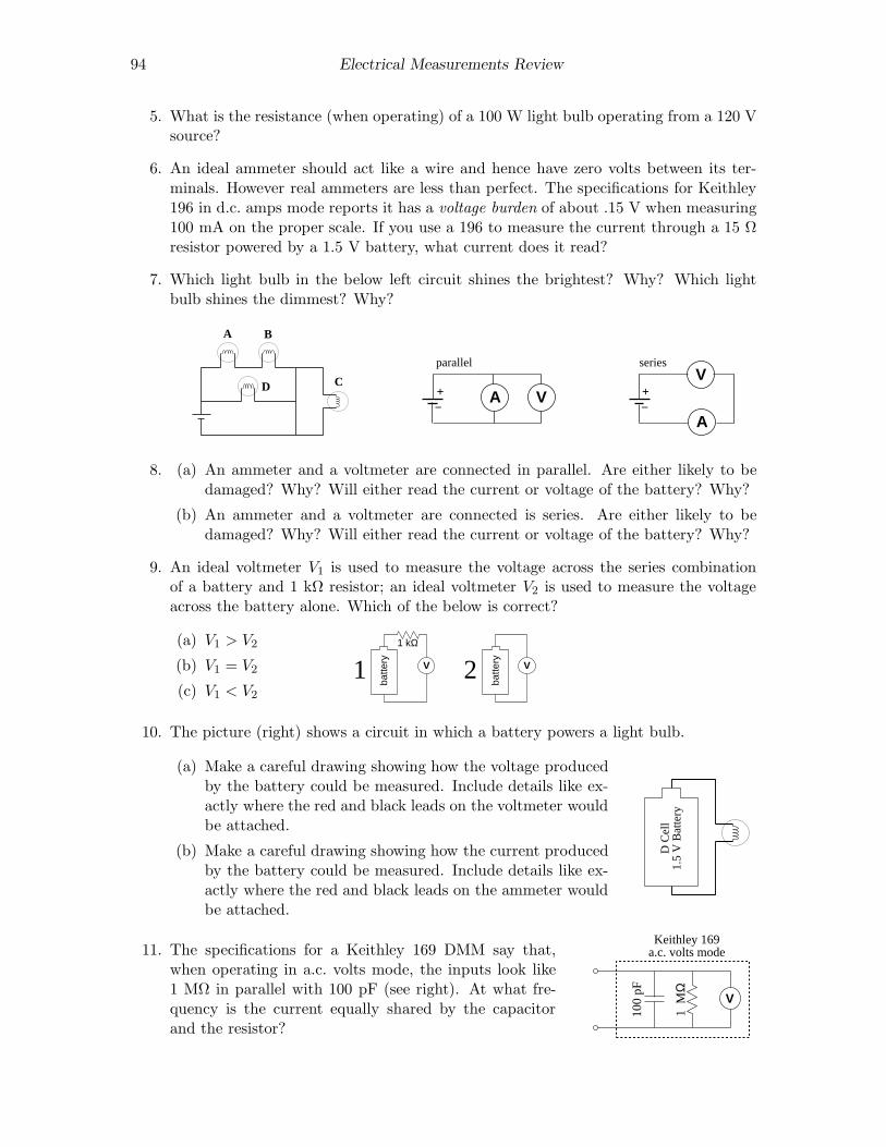
94 Electrical Measurements Review

5. What is the resistance (when operating) of a 100 W light bulb operating from a 120 Vsource?

6. An ideal ammeter should act like a wire and hence have zero volts between its ter-minals. However real ammeters are less than perfect. The specifications for Keithley196 in d.c. amps mode reports it has a voltage burden of about .15 V when measuring100 mA on the proper scale. If you use a 196 to measure the current through a 15 Ωresistor powered by a 1.5 V battery, what current does it read?

7. Which light bulb in the below left circuit shines the brightest? Why? Which lightbulb shines the dimmest? Why?

A B

CD +−

AV

V +−

A

parallel series

8. (a) An ammeter and a voltmeter are connected in parallel. Are either likely to bedamaged? Why? Will either read the current or voltage of the battery? Why?

(b) An ammeter and a voltmeter are connected is series. Are either likely to bedamaged? Why? Will either read the current or voltage of the battery? Why?

9. An ideal voltmeter V1 is used to measure the voltage across the series combinationof a battery and 1 kΩ resistor; an ideal voltmeter V2 is used to measure the voltageacross the battery alone. Which of the below is correct?

(a) V1 > V2

(b) V1 = V2

(c) V1 < V2

batte

ry

batte

ryV V

1 kΩ

1 2

10. The picture (right) shows a circuit in which a battery powers a light bulb.

(a) Make a careful drawing showing how the voltage producedby the battery could be measured. Include details like ex-actly where the red and black leads on the voltmeter wouldbe attached.

(b) Make a careful drawing showing how the current producedby the battery could be measured. Include details like ex-actly where the red and black leads on the ammeter wouldbe attached.

D C

ell

1.5

V B

atte

ry

11. The specifications for a Keithley 169 DMM say that,when operating in a.c. volts mode, the inputs look like1 MΩ in parallel with 100 pF (see right). At what fre-quency is the current equally shared by the capacitorand the resistor?

1 M

Ω

100

pF

V

Keithley 169a.c. volts mode

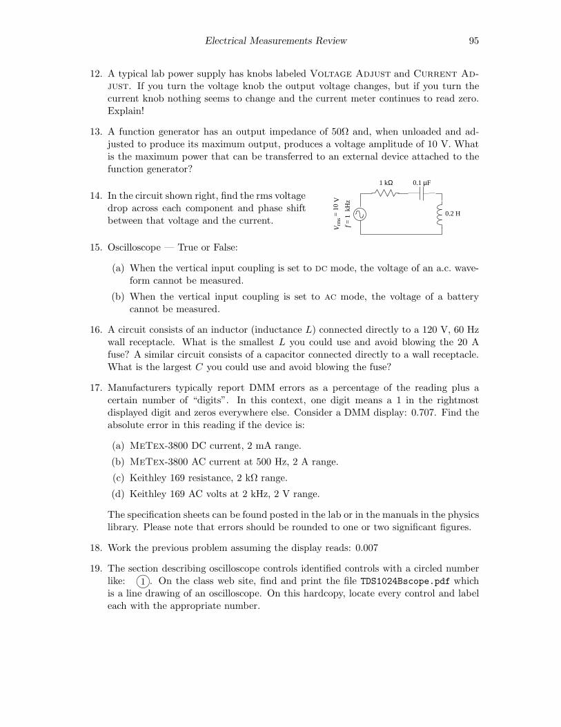
Electrical Measurements Review 95

12. A typical lab power supply has knobs labeled Voltage Adjust and Current Ad-just. If you turn the voltage knob the output voltage changes, but if you turn thecurrent knob nothing seems to change and the current meter continues to read zero.Explain!

13. A function generator has an output impedance of 50Ω and, when unloaded and ad-justed to produce its maximum output, produces a voltage amplitude of 10 V. Whatis the maximum power that can be transferred to an external device attached to thefunction generator?

14. In the circuit shown right, find the rms voltagedrop across each component and phase shiftbetween that voltage and the current.

0.1 µF

0.2 H

Vrm

s = 1

0 V

f = 1

kH

z

1 kΩ

15. Oscilloscope — True or False:

(a) When the vertical input coupling is set to dc mode, the voltage of an a.c. wave-form cannot be measured.

(b) When the vertical input coupling is set to ac mode, the voltage of a batterycannot be measured.

16. A circuit consists of an inductor (inductance L) connected directly to a 120 V, 60 Hzwall receptacle. What is the smallest L you could use and avoid blowing the 20 Afuse? A similar circuit consists of a capacitor connected directly to a wall receptacle.What is the largest C you could use and avoid blowing the fuse?

17. Manufacturers typically report DMM errors as a percentage of the reading plus acertain number of “digits”. In this context, one digit means a 1 in the rightmostdisplayed digit and zeros everywhere else. Consider a DMM display: 0.707. Find theabsolute error in this reading if the device is:

(a) MeTex-3800 DC current, 2 mA range.

(b) MeTex-3800 AC current at 500 Hz, 2 A range.

(c) Keithley 169 resistance, 2 kΩ range.

(d) Keithley 169 AC volts at 2 kHz, 2 V range.

The specification sheets can be found posted in the lab or in the manuals in the physicslibrary. Please note that errors should be rounded to one or two significant figures.

18. Work the previous problem assuming the display reads: 0.007

19. The section describing oscilloscope controls identified controls with a circled numberlike: 1m. On the class web site, find and print the file TDS1024Bscope.pdf whichis a line drawing of an oscilloscope. On this hardcopy, locate every control and labeleach with the appropriate number.

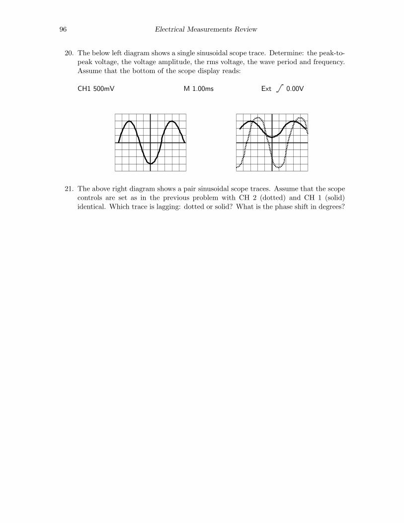
96 Electrical Measurements Review

20. The below left diagram shows a single sinusoidal scope trace. Determine: the peak-to-peak voltage, the voltage amplitude, the rms voltage, the wave period and frequency.Assume that the bottom of the scope display reads:

CH1 500mV M 1.00ms Ext 0.00V

21. The above right diagram shows a pair sinusoidal scope traces. Assume that the scopecontrols are set as in the previous problem with CH 2 (dotted) and CH 1 (solid)identical. Which trace is lagging: dotted or solid? What is the phase shift in degrees?

4: Electrical Measurements Lab

97

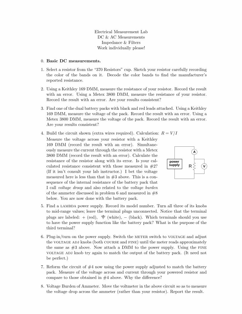
Electrical Measurement LabDC & AC MeasurementsImpedance & Filters

Work individually please!

0. Basic DC measurements.

1. Select a resistor from the “370 Resistors” cup. Sketch your resistor carefully recordingthe color of the bands on it. Decode the color bands to find the manufacturer’sreported resistance.

2. Using a Keithley 169 DMM, measure the resistance of your resistor. Record the resultwith an error. Using a Metex 3800 DMM, measure the resistance of your resistor.Record the result with an error. Are your results consistent?

3. Find one of the dual battery packs with black and red leads attached. Using a Keithley169 DMM, measure the voltage of the pack. Record the result with an error. Using aMetex 3800 DMM, measure the voltage of the pack. Record the result with an error.Are your results consistent?

4. Build the circuit shown (extra wires required). Calculation: R = V/I

Measure the voltage across your resistor with a Keithley169 DMM (record the result with an error). Simultane-ously measure the current through the resistor with a Metex3800 DMM (record the result with an error). Calculate theresistance of the resistor along with its error. Is your cal-culated resistance consistent with those measured in #2?(If it isn’t consult your lab instructor.) I bet the voltagemeasured here is less than that in #3 above. This is a con-sequence of the internal resistance of the battery pack thatI call voltage droop and also related to the voltage burdenof the ammeter discussed in problem 6 and measured in #8below. You are now done with the battery pack.

A

VRpowersupply

5. Find a lambda power supply. Record its model number. Turn all three of its knobsto mid-range values; leave the terminal plugs unconnected. Notice that the terminal

plugs are labeled: + (red), (white), − (black). Which terminals should you useto have the power supply function like the battery pack? What is the purpose of thethird terminal?

6. Plug-in/turn on the power supply. Switch the meter switch to voltage and adjustthe voltage adj knobs (both course and fine) until the meter reads approximatelythe same as #3 above. Now attach a DMM to the power supply. Using the finevoltage adj knob try again to match the output of the battery pack. (It need notbe perfect.)

7. Reform the circuit of #4 now using the power supply adjusted to match the batterypack. Measure of the voltage across and current through your powered resistor andcompare to those obtained in #4 above. Why the difference?

8. Voltage Burden of Ammeter. Move the voltmeter in the above circuit so as to measurethe voltage drop across the ammeter (rather than your resistor). Report the result.

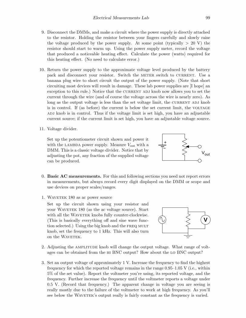
Electrical Measurements Lab 99

9. Disconnect the DMMs, and make a circuit where the power supply is directly attachedto the resistor. Holding the resistor between your fingers carefully and slowly raisethe voltage produced by the power supply. At some point (typically > 20 V) theresistor should start to warm up. Using the power supply meter, record the voltagethat produced a noticeable heating effect. Calculate the power (watts) required forthis heating effect. (No need to calculate error.)

10. Return the power supply to the approximate voltage level produced by the batterypack and disconnect your resistor. Switch the meter switch to current. Use abanana plug wire to short circuit the output of the power supply. (Note that shortcircuiting most devices will result in damage. These lab power supplies are [I hope] anexception to this rule.) Notice that the current adj knob now allows you to set thecurrent through the wire (and of course the voltage across the wire is nearly zero). Aslong as the output voltage is less than the set voltage limit, the current adj knobis in control. If (as before) the current is below the set current limit, the voltageadj knob is in control. Thus if the voltage limit is set high, you have an adjustablecurrent source; if the current limit is set high, you have an adjustable voltage source.

11. Voltage divider.

Set up the potentiometer circuit shown and power itwith the lambda power supply. Measure Vout with aDMM. This is a classic voltage divider. Notice that byadjusting the pot, any fraction of the supplied voltagecan be produced.

+−

Vout

0. Basic AC measurements. For this and following sections you need not report errorsin measurements, but always record every digit displayed on the DMM or scope anduse devices on proper scales/ranges.

1. Wavetek 180 as ac power source

Set up the circuit shown using your resistor andyour Wavetek 180 (as the ac voltage source). Startwith all the Wavetek knobs fully counter-clockwise.(This is basically everything off and sine wave func-tion selected.) Using the big knob and the freq multknob, set the frequency to 1 kHz. This will also turnon the Wavetek.

V

2. Adjusting the amplitude knob will change the output voltage. What range of volt-ages can be obtained from the hi BNC output? How about the lo BNC output?

3. Set an output voltage of approximately 1 V. Increase the frequency to find the highestfrequency for which the reported voltage remains in the range 0.95–1.05 V (i.e., within5% of the set value). Report the voltmeter you’re using, its reported voltage, and thefrequency. Further increase the frequency until the voltmeter reports a voltage under0.5 V. (Record that frequency.) The apparent change in voltage you are seeing isreally mostly due to the failure of the voltmeter to work at high frequency. As you’llsee below the Wavetek’s output really is fairly constant as the frequency is varied.

100 Electrical Measurements Lab

4. With the output voltage still set at approximately 1 V, set the frequency to 100 Hz,and measure the ac current through and the ac voltage across your resistor. (Therequired circuit is analogous to #4 above. You might want to have your instructorcheck your circuit before powering up.) Calculate the resistance (no error calculationrequired). Your result should be consistent with previous resistance measurements.Measure the current again at a frequency of 1 kHz. Does the current (and henceresistance) vary much with frequency?

5. Replace your resistor with a capacitor. With the 100 Hz, 1 V output, measure thecurrent and voltage. Calculate the “resistance” (actually reactance, i.e., V/I). Usingyour calculated reactance, calculate the capacitance (see Fig. 3.1 on page 82 if you’reunsure of the definition of C). Measure again at a frequency of 1 kHz. Does the current(and hence reactance) vary much with frequency? Again calculate the capacitance—itshould be nearly the same even though the current should be nearly ten times bigger.

0. Basic scope measurements. Note: A “scope trace sketch” should include: hor-izontal and vertical scale settings (and the size of a div on your sketch—this is oneplace where quad ruled notebook paper helps!), the location of ground (zero volts),and the signal frequency. All of these numbers are on the scope display. In additionreport the type of Coupling being used on the displayed channel. Feel free to report“same settings as previous” if that is the case.

1. Set up the scope and a DMM to monitor the functiongenerator as shown. Set the function generator toproduce a ∼1 V sine wave at a frequency of ∼1 kHz.Turn on the scope and hit default setup. You mustnow change both CH1 and CH2 to 1× probe from thedefault value of 10× probe. Fiddle (or not) with thecontrols until you have a nice stable display of thesignal on the scope. Sketch the scope trace.

V

scop

e

2. Record the size (in units of divisions on the display) for: the peak-to-peak voltage(Vpp), the amplitude or peak voltage (Vp), and the period (T ) of the wave. Convertthese to physical units (volts, seconds) using the scale factors. Calculate the frequencyfrom the period and compare to the set value. Calculate the rms voltage from thepeak voltage and compare to the DMM value. Hit the measure menu and arrangethe simultaneous display of Freq, Period, Pk-Pk voltage, Cyc RMS voltage, and Maxvoltage. Compare these values to those you calculated from divisions.

3. Run the function generator frequency up to and beyond the limiting value determinedin previous section, #3. Notice that the scope (correctly) shows a constant amplitudeeven as the voltmeter (incorrectly) shows a varying voltage.

4. Return the frequency to 1 kHz. Vary the function produced by the function generator:try triangle and square waves. For each wave, record the scope-reported peak-to-peakand rms voltages. Also record the rms voltage reported by the DMM. For a squarewave: Vrms = Vpp/2; for a triangle wave: Vrms = Vpp/2

√3. Compare these calculated

rms voltages to those directly reported by the scope and DMM. Which device appearsto be a “true rms” meter? Explain.

Electrical Measurements Lab 101

5. In the measure menu change the measurement of Period to Mean (voltage). Find thedc offset knob on the function generator. Monitor the scope display and producea ∼1 V amplitude sine wave with a ∼1 V dc offset. Sketch the resulting scope trace.Record the DMM ac voltmeter reading; record the scope Cyc RMS voltage. Switchthe DMM to dc volts and record the dc voltage the reading; record the scope Meanvoltage.

Switch the scope’s input to CouplingAC, and repeat the above sketches and mea-surements. Comment on the results.

0. Filters.

In many circumstances in electronics we are concerned with the ratio of voltages (orpowers, currents, etc.), e.g., A ≡ Vout/Vin. For example the aim of an amplifier is toproduce a Vout ≫ Vin and one is usually primarily concerned with the amplification (orgain), which is that ratio. (A > 1 for amplification.) On the other hand, sunglassesaim to reduce or attenuate light before in enters the eye. (A < 1 for attenuation.)Such ratios are most often reported in decibels (dB):

20 log10 (Vout/Vin) (4.1)

Thus if an amplifier increases the voltage by a factor of 10 (i.e., A = 10), we wouldsay the amplifier has a gain of 20 dB. Some common examples:

amplification attenuationA dB A dB

100 40 1100 −40

10 20 110 −20

2 6 12 −6√

2 3 1√2

−3

1 0 1 0

An electronic filter aims to pass certain frequencies and attenuate others. For example,a radio antenna naturally picks up every frequency; an electronic filter must attenuateall but the desired frequency. We start here with a low pass filter : a filter that lets lowfrequencies pass nearly untouched, but attenuates high frequencies. It is impossibleto have step changes in attenuation, so as the frequency is increased, A goes smoothlyto zero. Traditionally the curve of A vs. f is presented as a log-log plot and is calleda Bode1 plot. Filters are usually characterized by their “−3 dB” frequency (f−3dB),i.e., the frequency2 at which A = 1/

√2 ≈ .707.

For the following measurements you will use a sinusoidal signal with no dc offset anda very large range of frequencies and voltages: Remember to adjust your scope scalesappropriately. Your voltage measurements are most easily done as Pk-Pk or CycRMS (it doesn’t matter which, just be consistent) with CouplingAC.

1. Solder together a lead from your resistor and a lead from your capacitor.

1“Bo–Dee” plots were popularized by Hendrik Wade Bode’s book Network Analysis and Feedback Am-

plifier Design 1945. Bode worked at Bell Labs and became head of the lab’s Mathematics Department in1944.

2Note: The general definition of f−3dB is not that the gain is .707, rather that the gain has changed

from some standard value by a factor of .707, i.e., the gain is 3 dB less than ‘usual’. In #2 the ‘usual’ A is1, so f−3dB is where A = .707 In #3 the ‘usual’ A is .5, so f−3dB is where A = .354

102 Electrical Measurements Lab

2. RC low pass filter.

Use your RC combination to construct the low passfilter shown. You will monitor the input to the filter(Vin) on ch 2 of the scope and the output (Vout) on ch1. Describe how this filter’s ‘gain’ (but here A < 1,so ‘attenuation’ might be a better word) changes asthe frequency is varied from 50 Hz to 1 MHz. Findthe filter’s f−3dB (at which Vout = Vin/

√2 ). Make a

table of attenuation (Vout/Vin), dB, and f measuredat frequencies of about 0.1, 0.2, 1, 2, 10, 20, and 100times f−3dB. (Note that if, by adjusting the ampli-tude on the Wavetek you make Vin = 1, you won’tneed a calculator to find Vout/Vin.) By hand, makea log-log graph of attenuation vs. f using the sup-plied paper. Check that the filter’s Bode-plot slopefor f > f−3dB is 6 dB per octave (or, equivalently, 20dB per decade). Sketch (together) the scope tracesat f−3dB. Does Vout lead or lag Vin? (Note: a RClow pass filter is behind your scope’s HF Reject op-tion; a RC high pass filter is behind your scope’sCouplingAC option.)

Vout

Vin

3. LC Filter

I’ve constructed the beastie shown. (For the curious, it’s a 5-pole, low-pass But-terworth filter in the π-configuration: see Appendix H of Horowitz and Hill if youwant more details.) At low frequencies the gain never exceeds about 1

2 ; thereforef−3dB is defined as the frequency at which A is .707× its low frequency value, i.e.,A = .707 × .5 = .354. Using a sine wave as input, take data of attenuation vs. fre-quency and plot them on log-log paper. Use frequencies of about 0.01, 0.1, 0.2, 0.5, 1,2, 4, and 8 times f−3dB. (At high frequencies the attenuation is so large that Vout maybe lost in the noise unless you increase Vin to well above 1 V.) How does the steepnessof this filter’s cut-off compare with that of the simple RC filter? (I.e., compare thedB-per-octave falloff of this filter to the simple RC filter.)

.01 µF .033 µF .01 µF

500 Ω 10 mH 10 mH

560 Ω

VoutVin

4. Tape your resistor+capacitor combination in your notebook.

5: Thermionic Emission

Purpose

While we think of quantum mechanics being best demonstrated in processes that showdiscontinuous change, historically quantum mechanics was first revealed in systems wherea large number of particles washed out the jumps: blackbody radiation and thermionicemission. In this lab you will investigate these two phenomena in addition to classicalspace-charge limited electron emission: Child’s Law.

Introduction

Metals, as demonstrated by their ability to conduct an electric current, contain mobileelectrons. (Most electrons in metals, particularly the “core” electrons closest to the nucleus,are tightly bound to individual atoms; it is only the outermost “valence” electrons that aresomewhat “free”.) These free electrons are generally confined to the bulk of the metal. Asyou learned in E&M, an electron attempting to leave a conductor experiences a strong forceattracting it back towards the conductor due to an image charge:

Fx = − e2

4πǫ0(2x)2(5.1)

where x is the distance the electron is from the interface and e is the absolute value of thecharge on an electron. Of course, inside the metal the electric field is zero so an electronthere experiences zero (average) force. You can think of these valence electrons as bouncingaround inside a box whose “walls” are provided by the image-charge force. (Odd to think:the “walls” are non-material force fields; the “inside” of the box is filled with solid metal.)Since temperature is a measure of random kinetic energy, if we increase the temperature ofthe metal, the electrons will be moving faster and some will have enough energy to overcomethe image-charge force (which after all becomes arbitrarily small at large distances from theinterface) and escape. This is electron “evaporation”. The higher the temperature thelarger the current of escaping electrons. This temperature induced electron flow is calledthermionic emission. Starting in 1901, Owen Richardson studied this phenomenon and in1929 he received the Nobel prize in Physics for his work.

A hot wire will be surrounded by evaporated electrons. An electric force can pull theseelectrons away from the wire — the larger the electric force, the larger the resulting currentof electrons. The precise relationship between the voltage and the resulting current flow

103

104 Thermionic Emission

&&&&&&&&&&&&&&&&&&&&&&&&&&&&&&&&&&&&&&&&&&&&&&&&&&&&&&&&&&&&&&&&&&&&&&&&&&&&&&&&&&&&&&&&&&&&&&&&&&&&&&&&&&&&&&&&

metal

vacuum anodecathode

xx = bx = 0

acceleratingelectrons

electric currentdensity JA

VAV = 0

Figure 5.1: A planar cathode and a planar anode are separated by a distance b. A positivepotential difference VA attracts electrons from the cathode to the anode, so the speed of theelectrons v(x) increases as they approach the anode. The moving electrons constitute anelectric current from anode to cathode. The resulting steady current density is called JA.

is called Child’s law1 (or the Child-Langmuir law, including Langmuir who independentlydiscovered it while working at G.E.). In this experiment you will measure both Child’s Lawand the Richardson Effect.

Child’s Law

Consider a planar interface between a metal (x < 0) and “vacuum” (x > 0). Vacuum isin quotes because this region will contain escaped electrons—a ‘space charge’—rather thanbeing totally empty2. The number of electrons per volume (i.e., the number density) isdenoted by n.

In this experiment, the metal will be heated (i.e., its a ‘hot cathode’ or filament) which willresult in a supply of electrons ‘evaporated’ from the metal into the vacuum. An additionalconducting sheet (the anode) is located at x = b. A positive potential difference, VA,between the cathode and the anode plane provides a force pulling these electrons from thevicinity of the cathode towards the anode. The result is a stream of moving electrons (acurrent); the number density n(x) and speed v(x) of these electrons will depend on location,x, between the plates. The negatively charged electrons moving to the right constitute asteady electric current density to the left, i.e., a steady conventional electric current fromthe anode to the cathode:

J = −en(x)v(x) = −JA (5.2)

Since the electrons leave the metal with (nearly) zero speed at zero potential, we cancalculate their speed along the path to the anode using conservation of energy:

1

2mv2 − eV (x) = 0 (5.3)

v =

√

2e

mV (x) (5.4)

1Clement Dexter Child (1868–1933) Born: Madison, Ohio, A.B. Rochester, Ph.D. Cornell2In fact a perfect vacuum is not possible, so the word “vacuum” actually refers simply to a region with

relatively few particles per volume

Thermionic Emission 105

where V (x) is the potential difference (“voltage”) at x and m is the mass of an electron.Because the accelerating electrons constitute a steady current (i.e., JA doesn’t dependon position), n(x) must decrease as the electrons speed toward the anode. The varyingspace charge density affects the electric potential in the “vacuum” according to Poisson’sequation3:

∂2V

∂x2= −ρ(x)

ǫ0=en(x)

ǫ0(5.5)

Putting these pieces together with have the differential equation:

d2V

dx2=

JAǫ0v(x)

=JA

ǫ0

√

2em V (x)

(5.6)

Since the electric field will be zero at the interface, we have a pair of initial conditions:

∂V

∂x

∣

∣

∣

∣

x=0

= 0 (5.7)

V |x=0 = 0 (5.8)

This differential equation looks a bit like Newton’s second law:

d2x

dt2=

1

mF (x(t)) (5.9)

as you can see if in Newton’s second law you substitute:

t −→ x

x(t) −→ V (x)

1

mF (x(t)) −→ JA

ǫ0

√

2em V (x)

Recall that force problems are often most simply solved using conservation of energy andthat conservation of energy was proved using an integrating factor of dx/dt. If we try theanalogous trick on our voltage problem, we’ll multiply Poisson’s equation by dV/dx:

dV

dx× d2V

dx2=

JA

ǫ0

√

2em

V − 1

2 × dV

dx(5.10)

(

1

2

[

dV

dx

]2)′

=JA

ǫ0

√

2em

(

V1

2

12

)′

(5.11)

1

2

[

dV

dx

]2

=JA

ǫ0

√

2em

V1

2

12

+ constant (5.12)

The initial conditions require the constant to be zero, so

1

2

[

dV

dx

]2

=JA

ǫ0

√

2em

V1

2

12

(5.13)

3Poisson’s equation is derived in the Appendix to this lab.

106 Thermionic Emission

ordV

dx=

√

√

√

√

4JA

ǫ0

√

2em

V1

4 (5.14)

This differential equation is separable:

dV

V1

4

=

√

√

√

√

4JA

ǫ0

√

2em

dx (5.15)

V3

4

34

=

√

√

√

√

4JA

ǫ0

√

2em

x (5.16)

where again the initial conditions require the constant of integration to be zero. Finally:

V (x) =

9JA

4ǫ0

√

2em

2

3

x4

3 (5.17)

Of course, V (b) is the anode voltage VA, so we can rearrange this equation to show Child’slaw:

JA =

[

4ǫ09b2

√

2e

m

]

V3

2

A (5.18)

Much of Child’s law is just the result of dimensional analysis, i.e., seeking any possibledimensionally correct formula for JA. Our differential equation just involves the followingconstants with dimensions (units) as shown:

b : L (5.19)

VA :E

Q=ML2/T 2

Q(5.20)

ǫ0

√

2e

m≡ k :

Q2

EL

Q1

2

M1

2

=Q

5

2

M3

2L3/T 2(5.21)

JA :Q/T

L2(5.22)

where the dimensions are: L=length, T=time, M=mass, E=energy, and Q=charge. Tomake a dimensionally correct formula for JA, we just eliminate the M dimension which wecan only do with the combination:

VAk2

3 :Q

2

3

T2

3

(5.23)

We can then get the right units for JA with:

(

VAk2

3

)3

2

b2=

k

b2V

3

2

A :Q/T

L2(5.24)

Thus the only possible dimensionally correct formula is

JA ∝ k

b2V

3

2

A (5.25)

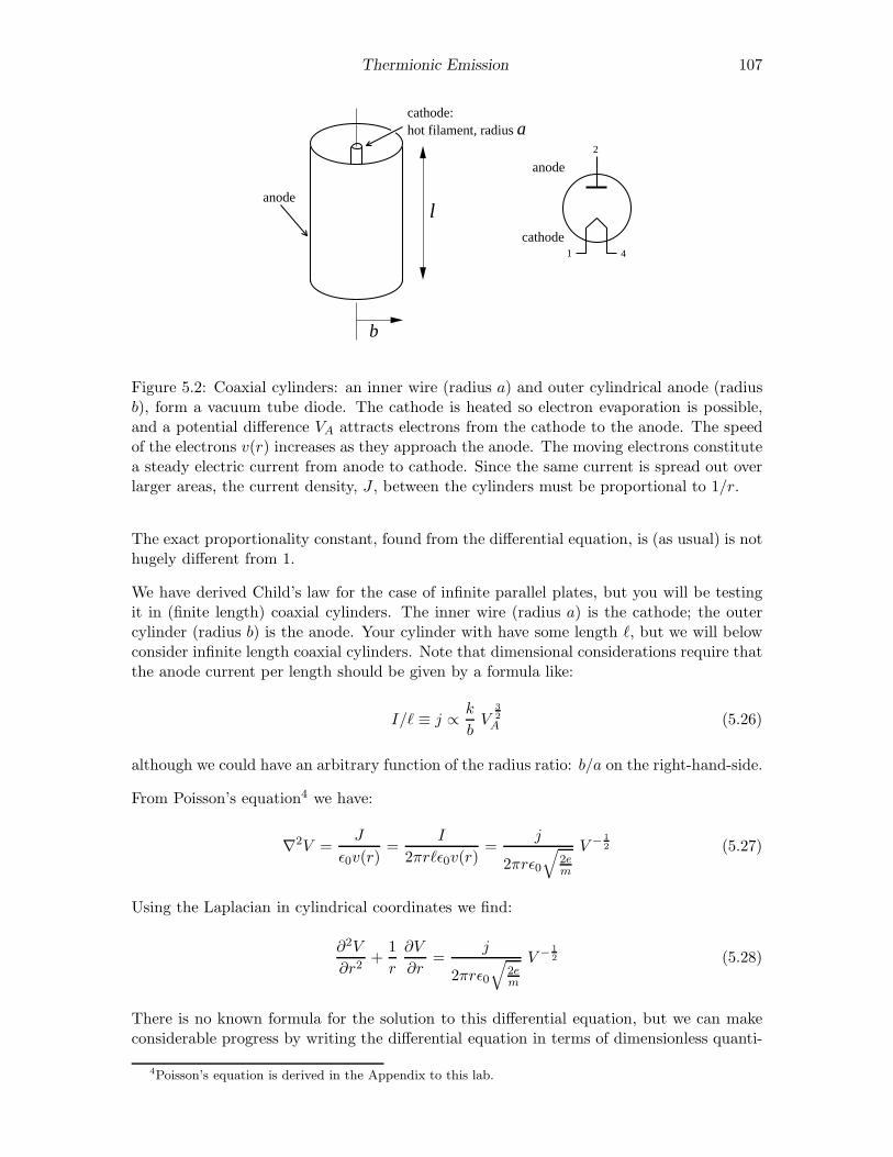
Thermionic Emission 107

l

b

anode

cathode:hot filament, radius a

anode

cathode1 4

2

Figure 5.2: Coaxial cylinders: an inner wire (radius a) and outer cylindrical anode (radiusb), form a vacuum tube diode. The cathode is heated so electron evaporation is possible,and a potential difference VA attracts electrons from the cathode to the anode. The speedof the electrons v(r) increases as they approach the anode. The moving electrons constitutea steady electric current from anode to cathode. Since the same current is spread out overlarger areas, the current density, J , between the cylinders must be proportional to 1/r.

The exact proportionality constant, found from the differential equation, is (as usual) is nothugely different from 1.

We have derived Child’s law for the case of infinite parallel plates, but you will be testingit in (finite length) coaxial cylinders. The inner wire (radius a) is the cathode; the outercylinder (radius b) is the anode. Your cylinder with have some length ℓ, but we will belowconsider infinite length coaxial cylinders. Note that dimensional considerations require thatthe anode current per length should be given by a formula like:

I/ℓ ≡ j ∝ k

bV

3

2

A (5.26)

although we could have an arbitrary function of the radius ratio: b/a on the right-hand-side.

From Poisson’s equation4 we have:

∇2V =J

ǫ0v(r)=

I

2πrℓǫ0v(r)=

j

2πrǫ0

√

2em

V − 1

2 (5.27)

Using the Laplacian in cylindrical coordinates we find:

∂2V

∂r2+

1

r

∂V

∂r=

j

2πrǫ0

√

2em

V − 1

2 (5.28)

There is no known formula for the solution to this differential equation, but we can makeconsiderable progress by writing the differential equation in terms of dimensionless quanti-

4Poisson’s equation is derived in the Appendix to this lab.

108 Thermionic Emission

ties:

r/a = ρ (5.29)

V =

ja

2πǫ0

√

2em

2

3

f(ρ) (5.30)

yielding:∂2f

∂ρ2+

1

ρ

∂f

∂ρ= f ′′(ρ) +

1

ρf ′(ρ) =

1

ρf−

1

2 (5.31)

with initial conditions:

f(1) = 0 (5.32)

f ′(1) = 0 (5.33)

We can numerically solve this differential equation using Mathematica:

NDSolve[f’’[p]+f’[p]/p==1/(p Sqrt[f[p]]), f[1]==0, f’[1]==0, f,p,1,200]

It’s actually not quite that simple. The cathode, at ρ = 1, is actually a singular point ofthe differential equation (i.e., f ′′(1) = ∞). However the situation very near the cathode iswell approximated by the planar case, where we’ve shown:

V (x) =

9JA

4ǫ0

√

2em

2

3

x4

3 =

9I

2πaℓ4ǫ0

√

2em

2

3

(r − a)4

3 =

9ja

2π4ǫ0

√

2em

2

3(

r − a

a

)4

3

=

[

9

4

]2

3

ja

2πǫ0

√

2em

2

3(

r − a

a

)4

3

(5.34)

So, near the cathode (i.e., ρ slightly larger than 1):

f(ρ) ≈[

9

4

]2

3

(ρ− 1)4

3 (5.35)

We can use this approximation to start our numerical differential equation solution at anon-singular point (like ρ = 1.00001).

Real devices are designed with b/a = ρanode ≫ 1. The behavior of f for large ρ can bedetermined by finding constants A and α for which f = Aρα is a solution to the differentialequation. One finds:

f =

(

9

4ρ

)2

3

(5.36)

A useful approximation for the range: 100 < b/a < 1000 is:

f =

(

9

4ρ

)2

3

+ 2 (5.37)

Thermionic Emission 109

50 100 150 200

10

20

30

40

50

60

ρ

f

2 4 6 8 10 12 14

2

4

6

8

10

ρ

f(ρ) exact

f(ρ) for ρ→∞

f(ρ) for ρ→1

Figure 5.3: The plot on the left displays the dimensionless voltage f obtained by numericalsolution to the differential equation. The plot on the right compares various approximationsfor f to this numerical solution.

(For example, the device used in lab has b/a = 121.5. For this value, the differentialequation gives f = 44.136; the above approximation gives: f = 44.130.)

We recover Child’s law by rearranging (5.30):

2πǫ0

√

2em

a

[

VAf(b/a)

]3

2

= j = I/ℓ (5.38)

Note: Langmuir’s original work (Phys. Rev. 22, 347 (1923)) on this subject is expressed interms of β where:

β2(ρ) ≡ 4

9

f3

2

ρ=

−→ρ→1 (ρ− 1)2

−→ρ→∞ 1

(5.39)

So:

8πǫ0ℓ√

2em

9bβ2V

3

2

A = I (5.40)

β2 = 1.072 for the device used in lab.

Richardson’s Law

Most any thermal process is governed by the Boltzmann factor:

exp

(

−∆E

kT

)

= e−∆E/kT (5.41)

where k is the Boltzmann constant. Approximately speaking the Boltzmann factor ex-presses the relative probability for an event requiring energy ∆E in a system at (absolute)temperature T . Clearly if ∆E ≫ kT , the probability of the event happening is low. If anelectron requires an energy W (called the work function) to escape from the metal, The

110 Thermionic Emission

Boltzmann factor suggests that this would happen with relative probability e−W/kT . Thusyou should expect that the current emitted by a heated metal would follow:

I ∼ e−W/kT (5.42)

Clearly you should expect different elements to have different work functions, just as differ-ent atoms have different ionization potentials. What is surprising is that the proportionalityfactor in the above equation includes a universal constant — that is, a constant that just de-pends on the properties of electrons (and, most importantly, Planck’s constant, h) and doesnot depend on the type of material. (This situation is similar to that of blackbody radia-tion, in which photons rather than electrons are leaving a heated body, which was Planck’stopic in discovering his constant. We will take up this topic on page 115.) Thermionicemission probes the quantum state of the electrons statistically, whereas the photoelectriceffect probes much the same physics electron by electron. (The next level problem is toexplain why this universal constant (the Richardson constant, A) in fact does depend a biton the material.) To show:

J = AT 2e−W/kT (5.43)

where

A =4πemk2

h3= 1.2× 106A/m2K2 (5.44)

Quantum Theory: Free Electron Gas

Instead of thinking about electron particles bouncing around inside a box, de Broglie invitesus to consider standing waves of electron probability amplitude:

ψ = N exp(ikxx) exp(ikyy) exp(ikzz) = Neik·r (5.45)

Recall 5 that vector ~k is the momentum, p = mv, of the electron and ~ = h/2π. Periodicboundary conditions on the box (which we take to be a cube with one corner at the originand the diagonally opposite corner at the point r = (L,L,L)) require each component kito satisfy:

ki =2π niL

(5.46)

where each ni is an integer. Thus each wave function is specified by a triplet of integers: n =(nx, ny, nz), the n-vector. Applying Schrodinger’s equation, we find that this wavefunctionhas energy:

E(n) =~2k2

2m=

(2π~)2n2

2mL2=

(2π~)2(n2x + n2y + n2z)

2mL2(5.47)

Notice that there is a definite relationship between the velocity vector of the electron andthe n-vector.

v =2π~

mLn (5.48)

Another way of saying the same thing is that allowed quantum-state velocities form a cubiclattice with cube-side 2π~/mL. The number of states with electron velocities in somespecified region (for example a velocity-space parallelepiped with sides: ∆vx∆vy∆vz) can

5For a review see: http://britneyspears.ac/physics/dos/dos.htm

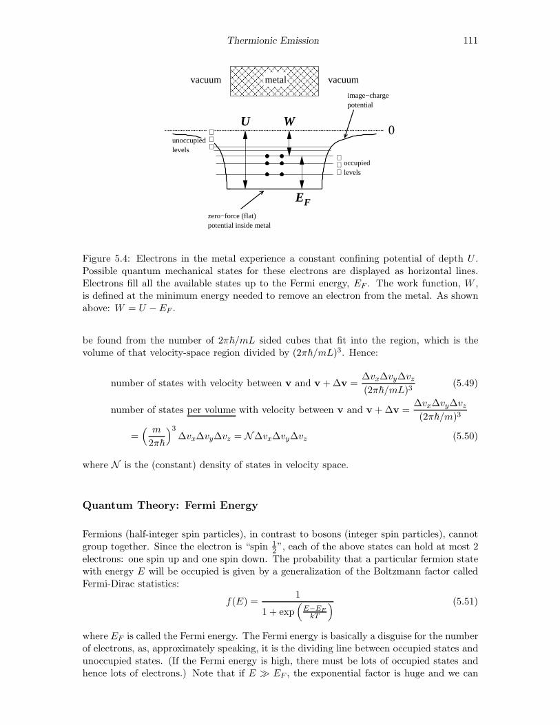
Thermionic Emission 111

&&&&&&&&&&&&&&&&&&&&&&&&&&&&&&&&&&&&&&&&&&&&&&&&&&&&&&&&&&&&&&&&&&&&&&&&&&&&&&&&&&&&&&&&&&&&&&&&

metal

0U W

EF

occupiedlevels

image−chargepotential

vacuumvacuum

zero−force (flat) potential inside metal

unoccupiedlevels

Figure 5.4: Electrons in the metal experience a constant confining potential of depth U .Possible quantum mechanical states for these electrons are displayed as horizontal lines.Electrons fill all the available states up to the Fermi energy, EF . The work function, W ,is defined at the minimum energy needed to remove an electron from the metal. As shownabove: W = U − EF .

be found from the number of 2π~/mL sided cubes that fit into the region, which is thevolume of that velocity-space region divided by (2π~/mL)3. Hence:

number of states with velocity between v and v +∆v =∆vx∆vy∆vz(2π~/mL)3

(5.49)

number of states per volume with velocity between v and v +∆v =∆vx∆vy∆vz(2π~/m)3

=( m

2π~

)3∆vx∆vy∆vz = N∆vx∆vy∆vz (5.50)

where N is the (constant) density of states in velocity space.

Quantum Theory: Fermi Energy

Fermions (half-integer spin particles), in contrast to bosons (integer spin particles), cannotgroup together. Since the electron is “spin 1

2”, each of the above states can hold at most 2electrons: one spin up and one spin down. The probability that a particular fermion statewith energy E will be occupied is given by a generalization of the Boltzmann factor calledFermi-Dirac statistics:

f(E) =1

1 + exp(

E−EF

kT

) (5.51)

where EF is called the Fermi energy. The Fermi energy is basically a disguise for the numberof electrons, as, approximately speaking, it is the dividing line between occupied states andunoccupied states. (If the Fermi energy is high, there must be lots of occupied states andhence lots of electrons.) Note that if E ≫ EF , the exponential factor is huge and we can

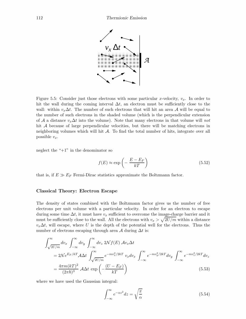
112 Thermionic Emission

A

CCCCCCCCCCCCCCCCCCCCCCCCCCCCCCCCCCCCCCCCCCCCCCCCCCCCCCCCCCCCCCCCCCCCCCCCCCCCCCCCCCCCCCCCCCCCCCCCCCCCCCCCCCCCCCCCCCCCCCCCCCCCCCCCCCCCCCCCCCCCCCCC

vx ∆t

Figure 5.5: Consider just those electrons with some particular x-velocity, vx. In order tohit the wall during the coming interval ∆t, an electron must be sufficiently close to thewall: within vx∆t. The number of such electrons that will hit an area A will be equal tothe number of such electrons in the shaded volume (which is the perpendicular extensionof A a distance vx∆t into the volume). Note that many electrons in that volume will nothit A because of large perpendicular velocities, but there will be matching electrons inneighboring volumes which will hit A. To find the total number of hits, integrate over allpossible vx.

neglect the “+1” in the denominator so

f(E) ≈ exp

(

− E − EF

kT

)

(5.52)

that is, if E ≫ EF Fermi-Dirac statistics approximate the Boltzmann factor.

Classical Theory: Electron Escape

The density of states combined with the Boltzmann factor gives us the number of freeelectrons per unit volume with a particular velocity. In order for an electron to escapeduring some time ∆t, it must have vx sufficient to overcome the image-charge barrier and itmust be sufficiently close to the wall. All the electrons with vx >

√

2U/m within a distancevx∆t, will escape, where U is the depth of the potential well for the electrons. Thus thenumber of electrons escaping through area A during ∆t is:

∫ ∞√

2U/mdvx

∫ ∞

−∞dvy

∫ ∞

−∞dvz 2N f(E) Avx∆t

= 2N eEF /kTA∆t

∫ ∞√

2U/me−mv2x/2kT vxdvx

∫ ∞

−∞e−mv2y/2kTdvy

∫ ∞

−∞e−mv2z/2kT dvz

=4πm(kT )2

(2π~)3A∆t exp

(

−(U − EF )

kT

)

(5.53)

where we have used the Gaussian integral:

∫ ∞

−∞e−αz2dz =

√

π

α(5.54)

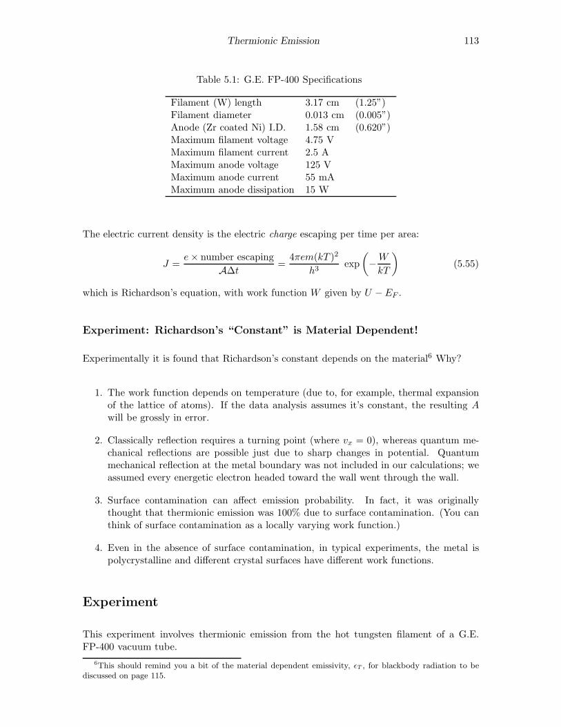
Thermionic Emission 113

Table 5.1: G.E. FP-400 Specifications

Filament (W) length 3.17 cm (1.25”)Filament diameter 0.013 cm (0.005”)Anode (Zr coated Ni) I.D. 1.58 cm (0.620”)Maximum filament voltage 4.75 VMaximum filament current 2.5 AMaximum anode voltage 125 VMaximum anode current 55 mAMaximum anode dissipation 15 W

The electric current density is the electric charge escaping per time per area:

J =e× number escaping

A∆t=

4πem(kT )2

h3exp

(

−W

kT

)

(5.55)

which is Richardson’s equation, with work function W given by U −EF .

Experiment: Richardson’s “Constant” is Material Dependent!

Experimentally it is found that Richardson’s constant depends on the material6 Why?

1. The work function depends on temperature (due to, for example, thermal expansionof the lattice of atoms). If the data analysis assumes it’s constant, the resulting Awill be grossly in error.

2. Classically reflection requires a turning point (where vx = 0), whereas quantum me-chanical reflections are possible just due to sharp changes in potential. Quantummechanical reflection at the metal boundary was not included in our calculations; weassumed every energetic electron headed toward the wall went through the wall.

3. Surface contamination can affect emission probability. In fact, it was originallythought that thermionic emission was 100% due to surface contamination. (You canthink of surface contamination as a locally varying work function.)

4. Even in the absence of surface contamination, in typical experiments, the metal ispolycrystalline and different crystal surfaces have different work functions.

Experiment

This experiment involves thermionic emission from the hot tungsten filament of a G.E.FP-400 vacuum tube.

6This should remind you a bit of the material dependent emissivity, ǫT , for blackbody radiation to bediscussed on page 115.

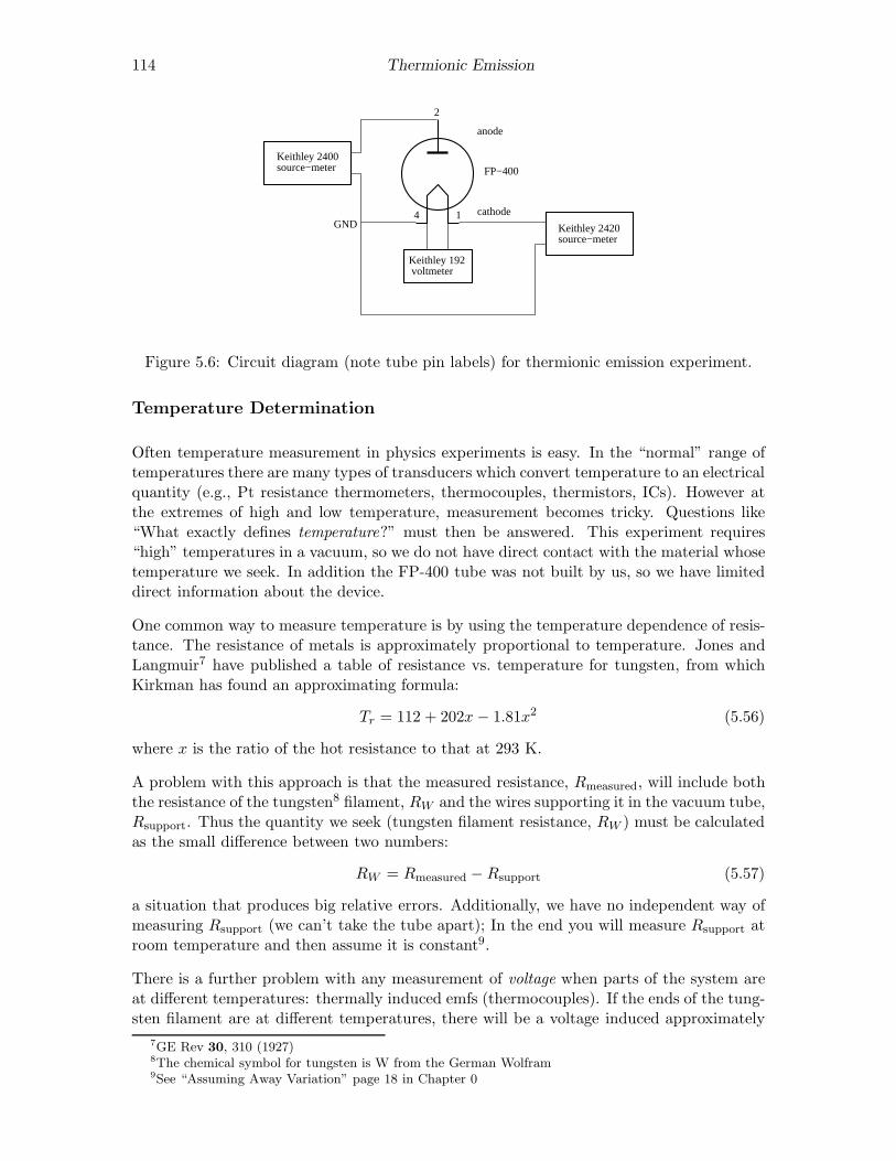
114 Thermionic Emission

4 1

2

Keithley 2400source−meter

Keithley 2420source−meter

Keithley 192 voltmeter

anode

cathodeGND

FP−400

Figure 5.6: Circuit diagram (note tube pin labels) for thermionic emission experiment.

Temperature Determination

Often temperature measurement in physics experiments is easy. In the “normal” range oftemperatures there are many types of transducers which convert temperature to an electricalquantity (e.g., Pt resistance thermometers, thermocouples, thermistors, ICs). However atthe extremes of high and low temperature, measurement becomes tricky. Questions like“What exactly defines temperature?” must then be answered. This experiment requires“high” temperatures in a vacuum, so we do not have direct contact with the material whosetemperature we seek. In addition the FP-400 tube was not built by us, so we have limiteddirect information about the device.

One common way to measure temperature is by using the temperature dependence of resis-tance. The resistance of metals is approximately proportional to temperature. Jones andLangmuir7 have published a table of resistance vs. temperature for tungsten, from whichKirkman has found an approximating formula:

Tr = 112 + 202x− 1.81x2 (5.56)

where x is the ratio of the hot resistance to that at 293 K.

A problem with this approach is that the measured resistance, Rmeasured, will include boththe resistance of the tungsten8 filament, RW and the wires supporting it in the vacuum tube,Rsupport. Thus the quantity we seek (tungsten filament resistance, RW ) must be calculatedas the small difference between two numbers:

RW = Rmeasured −Rsupport (5.57)

a situation that produces big relative errors. Additionally, we have no independent way ofmeasuring Rsupport (we can’t take the tube apart); In the end you will measure Rsupport atroom temperature and then assume it is constant9.

There is a further problem with any measurement of voltage when parts of the system areat different temperatures: thermally induced emfs (thermocouples). If the ends of the tung-sten filament are at different temperatures, there will be a voltage induced approximately

7GE Rev 30, 310 (1927)8The chemical symbol for tungsten is W from the German Wolfram9See “Assuming Away Variation” page 18 in Chapter 0

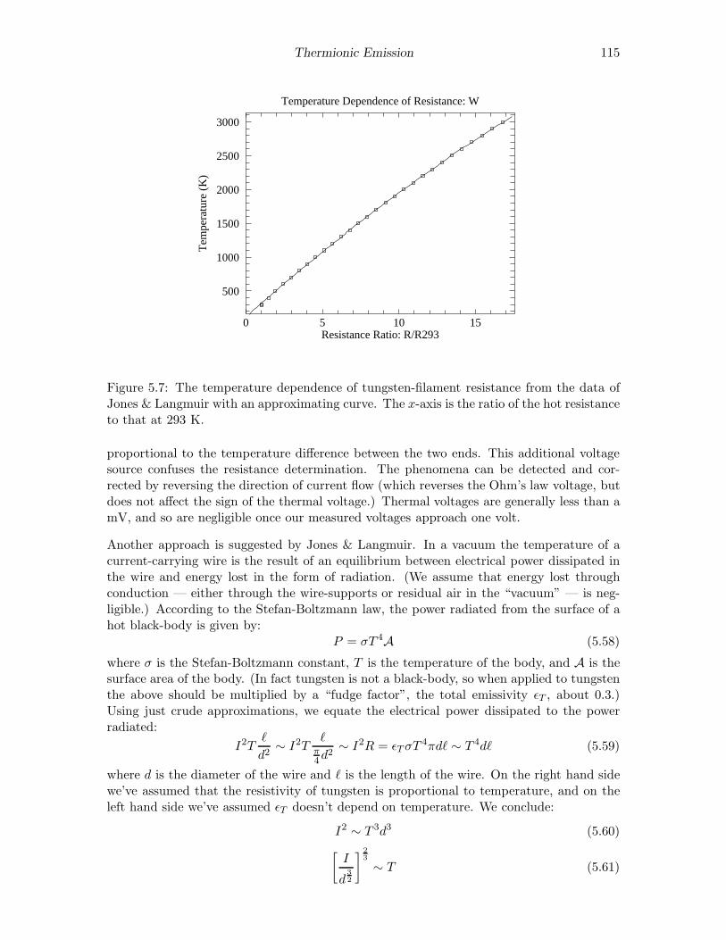
Thermionic Emission 115

0 5 10 15

3000

2500

2000

1500

1000

500

Temperature Dependence of Resistance: W

Resistance Ratio: R/R293

Tem

pera

ture

(K

)

Figure 5.7: The temperature dependence of tungsten-filament resistance from the data ofJones & Langmuir with an approximating curve. The x-axis is the ratio of the hot resistanceto that at 293 K.

proportional to the temperature difference between the two ends. This additional voltagesource confuses the resistance determination. The phenomena can be detected and cor-rected by reversing the direction of current flow (which reverses the Ohm’s law voltage, butdoes not affect the sign of the thermal voltage.) Thermal voltages are generally less than amV, and so are negligible once our measured voltages approach one volt.

Another approach is suggested by Jones & Langmuir. In a vacuum the temperature of acurrent-carrying wire is the result of an equilibrium between electrical power dissipated inthe wire and energy lost in the form of radiation. (We assume that energy lost throughconduction — either through the wire-supports or residual air in the “vacuum” — is neg-ligible.) According to the Stefan-Boltzmann law, the power radiated from the surface of ahot black-body is given by:

P = σT 4A (5.58)

where σ is the Stefan-Boltzmann constant, T is the temperature of the body, and A is thesurface area of the body. (In fact tungsten is not a black-body, so when applied to tungstenthe above should be multiplied by a “fudge factor”, the total emissivity ǫT , about 0.3.)Using just crude approximations, we equate the electrical power dissipated to the powerradiated:

I2Tℓ

d2∼ I2T

ℓπ4d

2∼ I2R = ǫTσT

4πdℓ ∼ T 4dℓ (5.59)

where d is the diameter of the wire and ℓ is the length of the wire. On the right hand sidewe’ve assumed that the resistivity of tungsten is proportional to temperature, and on theleft hand side we’ve assumed ǫT doesn’t depend on temperature. We conclude:

I2 ∼ T 3d3 (5.60)

[

I

d3

2

]2

3

∼ T (5.61)

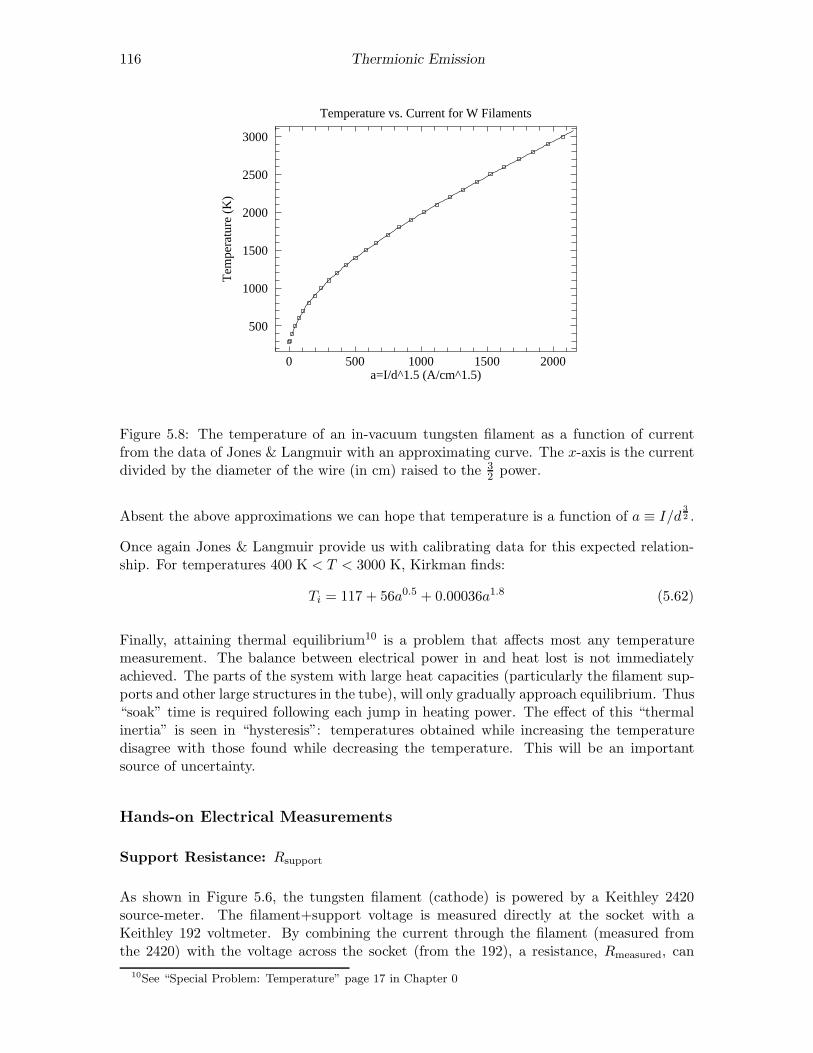
116 Thermionic Emission

0 500 1000 1500 2000

3000

2500

2000

1500

1000

500

Temperature vs. Current for W Filaments

a=I/d^1.5 (A/cm^1.5)

Tem

pera

ture

(K

)

Figure 5.8: The temperature of an in-vacuum tungsten filament as a function of currentfrom the data of Jones & Langmuir with an approximating curve. The x-axis is the currentdivided by the diameter of the wire (in cm) raised to the 3

2 power.

Absent the above approximations we can hope that temperature is a function of a ≡ I/d3

2 .

Once again Jones & Langmuir provide us with calibrating data for this expected relation-ship. For temperatures 400 K < T < 3000 K, Kirkman finds:

Ti = 117 + 56a0.5 + 0.00036a1.8 (5.62)

Finally, attaining thermal equilibrium10 is a problem that affects most any temperaturemeasurement. The balance between electrical power in and heat lost is not immediatelyachieved. The parts of the system with large heat capacities (particularly the filament sup-ports and other large structures in the tube), will only gradually approach equilibrium. Thus“soak” time is required following each jump in heating power. The effect of this “thermalinertia” is seen in “hysteresis”: temperatures obtained while increasing the temperaturedisagree with those found while decreasing the temperature. This will be an importantsource of uncertainty.

Hands-on Electrical Measurements

Support Resistance: Rsupport

As shown in Figure 5.6, the tungsten filament (cathode) is powered by a Keithley 2420source-meter. The filament+support voltage is measured directly at the socket with aKeithley 192 voltmeter. By combining the current through the filament (measured fromthe 2420) with the voltage across the socket (from the 192), a resistance, Rmeasured, can

10See “Special Problem: Temperature” page 17 in Chapter 0

Thermionic Emission 117

be determined. At room temperature, the filament resistance, RW , can be calculated fromthe filament geometry (see Table 5.1) and the resistivity of W-filament material at roomtemperature: ρ293 = 5.49 µΩ · cm. (You should calculate: RW ∼ .1 Ω.) Then:

Rsupport = Rmeasured −RW (5.63)

Because room temperature Rmeasured is ‘small’ (and hence error prone), you will makethree distinct measurements of it. Begin by sourcing 1 mA and then 10 mA into theroom temperature filament (using the 2420), reading the resulting voltages on the 192, andcalculating the corresponding Rmeasured. Follow up those two measurements with a four-terminal resistance measurement just using the 192. (If Rmeasured is substantially largerthan ∼ .2 Ω, confirm that you have firm, low-resistance contacts between the socket andthe tube. Working the socket-tube contact may be required to find the lowest resistancespot.)

Maximum Filament Current, 2420 Voltage Compliance Limit

Following your determination of Rsupport in a room temperature tube, check out the con-ditions required to stay just below the tube’s maximum ratings (4.75 V, 2.5 A). Using the2420, successively source filament currents of 2.0 A, 2.1 A, 2.2 A, . . . to directly determinethe maximum current you can use without exceeding the 4.75 V limit across the tube’sfilament. Note that at just below maximum conditions, the 2420 will probably need toproduce voltages above 4.75 V (because of the resistance of the external wires: the volt-age drop across the connecting wires is not zero). Record the maximum 2420 voltage andtube current allowed by the tube’s ratings; you will need these numbers in step #2 of yourcomputer program.

Data Collection Plan

You will be collecting two types of data at the same time: thermal characteristics of thefilament and the thermionic properties of the tube (anode current/voltage relationship).Starting at a filament current of 0.9 A, increase the current flowing through the filamentin steps of 0.1 A to a maximum current (found as described above, about 2.4 A) and thenreverse those steps down to a filament current 1.0 A. The up-sweep in filament currentfollowed by the down-sweep will allow you to test for hysteresis. At each step in current,allow the filament to approach thermal equilibrium (wait, say, 15 seconds) and then measurethe voltage across and current through the cathode/anode. Calculate filament temperaturetwo ways (Equations (5.56) and (5.62)). Average the two to estimate the temperature, anduse half the absolute value of the difference to estimate the uncertainty.

You see above a classic example of systematic error. The temperature is measured twodifferent ways. Direct application of error propagation formulas to these temperaturescalculated from 6-digit meter values would suggest small uncertainties. However the twotemperatures in fact disagree. If only one method had been used to measure temperature,we would have badly underestimated the error.

118 Thermionic Emission

T 4 vs. Power: Testing Stefan-Boltzmann

By conservation of energy we know that the power dumped into the filament (mostly fromelectrical heating, but also from other sources like radiation from the room temperatureenvironment to the filament) should equal the power out of the filament (from black-bodyradiation and other factors like conduction down the supports). Thus:

ǫTσAT 4 = I2RW + constant (5.64)

T 4 =1

ǫTσAI2RW + constant (5.65)

y = bx+ a (5.66)

A graph of T 4 vs. power should be a straight line from which you will determine ǫT . (Notethat the error in power is quite small, so we have properly used it as an x variable.) Inorder to test this relationship you will want to make a file containing the filament power,T 4 (use the average of the two temperatures: (T 4

i + T 4r )/2), and the error in T 4 (use half

the difference from the two temperatures: |T 4i − T 4

r |/2).

IA vs. VA: Testing Child and Richardson

You will collect anode current vs. voltage curves for each different filament (cathode) tem-perature. Use the Keithley 2400 to sweep the anode voltage logarithmically from 2 V to120 V. (Note the maximum limits for the anode: 0.055 A or 125 V. Do not exceed either!)

According to Child’s law, the anode current, IA, should increase in proportion to V3

2

A . Ofcourse, at sufficiently high voltage the current will be limited by the maximum electronevaporation rate, and a current plateau forms at a level given by Richardson’s law. Atthe maximum filament current (corresponding to the maximum filament temperature andevaporation rate), plateau formation occurs at very high voltage and you have the longestrun of data following Child’s law. Make a file containing VA, IA, and δIA which you canuse to fit to the Child’s law functional form:

IA = k1 (VA − k2)3

2 (5.67)

In addition, you will want to make a big continuous file containing: VA, IA at every temper-ature tested. The current plateaus can be extracted from this file and fit to the Richardsonrelationship:

IA = k1 AT 2 e−k2/T (5.68)

Computer Data Collection

As part of this experiment you will write a computer program to control the experiment.Plagiarism Warning : like all lab work, this program is to be your own work! Programsstrikingly similar to previous programs will alarm the grader. I understand that this willoften be a difficult and new experience. Please consult with me as you write the program,and test the program (with tube disconnected!) before attempting a final data-collectingrun.

Your program will control all aspects of data collection. In particular it will:

Thermionic Emission 119

0. Declare and define all variables.

1. Open (i.e., create integer nicknames—i.e., iunit—for) the enets gpib1 and gpib2.

2. Initialize meters—requires knowing the gpib primary address—i.e., iadd—of the me-ter and the iunit it is attached to. Get the status of each meter after you haveinitialized it.

(a) Each source-meter must be told the maximum voltage and current it may produceduring the experiment. Initialize the 2400 (anode voltage/current) for the tubemaximum ratings.

(b) Initialize the 2420 (filament voltage/current) for the near tube-maximum ratingsfound above11. In the following I assume the current maximum is 2.4 A, but itmay be different for your tube.

(c) Initialize the 192 for autorange DC voltage measurements.

3. Open the files:

(a) filament.dat (intended for: If , Vf , Tr, Ti of filament).

(b) stefanB.dat (intended for: power, T 4, δT 4 of filament).

(c) VI.dat (intended for: all VA, IA of anode, with comments (‘!’) for filamentIf , Tr, Ti).

(d) child.dat (intended for: VA, IA, δIA of anode at maximum filament current).

(e) child-.dat (like above but intended for a downsweep of anode voltage).

(f) rich.dat (intended for: Tr, Ti, IA — i.e., the estimated temperatures and thecorresponding maximum anode current for Richardson’s Law).

4. Tell the 2420 source-meter to source a filament current of 0.9 A.

5. Let the system sleep for 60 seconds to approach thermal equilibrium.

6. Do a sequence of measurements where the filament temperature is sequentially in-creased (i.e., a temperature up-sweep) with filament currents ranging from 0.9 A tosome maximum (e.g., 2.4 A) current in steps of 0.1 A.

(a) Tell the 2420 source-meter to source a filament current (If ).

(b) Let the system sleep for 15 seconds to approach thermal equilibrium.

(c) Request a logarithmic sweep of the anode voltage (controlled by the 2400 source-meter) from 2 V to 120 V. Receive the resulting arrays: VA and IA.

(d) Turn off the anode voltage.

(e) Repeat (a) thus receiving an updated version of the filament current (it will bevery close to the requested current).

(f) Read the 192 to get the filament voltage (Vf ).

(g) Using Eqs. (5.56) and (5.57), calculate Tr based on the calculated tube resistanceRmeasured, the calculated room temperature filament resistance and Rsupport.

(h) Calculate Ti from Eq. (5.62)

11See Hands-on Electrical Measurements, p. 116. Recall: the 2420 maximum voltage will need to be a bitabove 4.75 V. If you have not yet completed those measurements, temporarily initialize with 4.75 V.

120 Thermionic Emission

(i) Write a line to the file filament.dat reporting: If , Vf , Tr, Ti.

(j) Write a line to the file stefanB.dat reporting: filament power (RW I2f ), T

4, and

δT 4 (see p. 118).

(k) Write a comment line (i.e., starts with ‘!’) to the file VI.dat reporting filamentdata: If , Tr, Ti.

(l) Write the anode sweep data (one data-pair per line) in the file VI.dat.

(m) Write a line to the file rich.dat reporting Tr, Ti, IA. Use IA at VA=120 V as theestimated plateau current. (When the experiment is over, you will need estimateδIA based on hysteresis, and may need to delete IA values if, for example, thecurrent did not plateau or if cold emission substantially added to the plateaucurrent.)

(n) Increment the filament current by 0.1 A and return to (a).

7. Collect data for Child’s Law. Begin by repeating a normal anode sweep at the max-imum filament current; follow all the steps (a)–(m) outlined in 6 above. In addition,write the anode sweep data (VA, IA, δIA) in the file child.dat (one data-tripletper line). In this case, δIA will be calculated from the manufacturer’s specs: per-cent+digits; the fortran function eAk2400 can do this error calculation automatically.Now check for hysteresis by doing a reverse anode sweep: from 120 V down to 2 V.Write this reverse anode sweep data (VA, IA, δIA) in the file child-.dat.

8. Do a sequence of measurements where the filament temperature is decreased (i.e., atemperature down-sweep) by sequentially sourcing filament currents from one stepdown from maximum (e.g., 2.3 A) back to 1.0 A. Follow steps (a)–(m) used in thetemperature up-sweep (part 6 above) and then:

(n) decrement the filament current by 0.1 A and return to (a).

9. Turn off the output of the 2420.

10. Close all files.

Note that the 0.9 A filament current data is just trash collected so the 1.0 A filament currentdata is taken on a pre-warmed filament.

Observations

While the computer collects the data observe the light from the filament. (There is a 116”

diameter hole in the anode allowing light from the mid-point of the filament to escape.)Initially the filament will not appear to be incandescent (i.e., not a source of light at all:dark) so it may help to turn off the lab lights to better observe the beginning of visibleincandescence. According to the Stefan-Boltzmann law the light energy radiated dependson T 4, so small changes in T produce big changes in light intensity. In addition to changesin light intensity, you should look for the more subtle change in light color: from a dull redto a brilliant yellow. Record your observations! At what filament temperature did you firstsee the filament producing light?

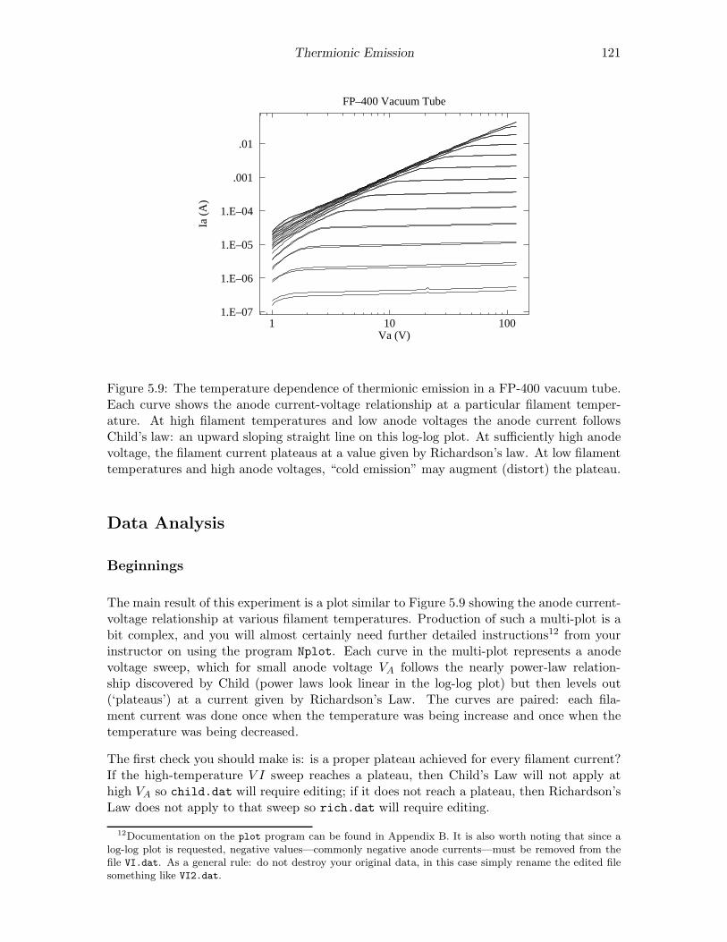
Thermionic Emission 121

1 10 100

.01

.001

1.E–04

1.E–05

1.E–06

1.E–07

FP–400 Vacuum Tube

Va (V)

Ia (

A)

Figure 5.9: The temperature dependence of thermionic emission in a FP-400 vacuum tube.Each curve shows the anode current-voltage relationship at a particular filament temper-ature. At high filament temperatures and low anode voltages the anode current followsChild’s law: an upward sloping straight line on this log-log plot. At sufficiently high anodevoltage, the filament current plateaus at a value given by Richardson’s law. At low filamenttemperatures and high anode voltages, “cold emission” may augment (distort) the plateau.

Data Analysis

Beginnings

The main result of this experiment is a plot similar to Figure 5.9 showing the anode current-voltage relationship at various filament temperatures. Production of such a multi-plot is abit complex, and you will almost certainly need further detailed instructions12 from yourinstructor on using the program Nplot. Each curve in the multi-plot represents a anodevoltage sweep, which for small anode voltage VA follows the nearly power-law relation-ship discovered by Child (power laws look linear in the log-log plot) but then levels out(‘plateaus’) at a current given by Richardson’s Law. The curves are paired: each fila-ment current was done once when the temperature was being increase and once when thetemperature was being decreased.

The first check you should make is: is a proper plateau achieved for every filament current?If the high-temperature V I sweep reaches a plateau, then Child’s Law will not apply athigh VA so child.dat will require editing; if it does not reach a plateau, then Richardson’sLaw does not apply to that sweep so rich.dat will require editing.

12Documentation on the plot program can be found in Appendix B. It is also worth noting that since alog-log plot is requested, negative values—commonly negative anode currents—must be removed from thefile VI.dat. As a general rule: do not destroy your original data, in this case simply rename the edited filesomething like VI2.dat.

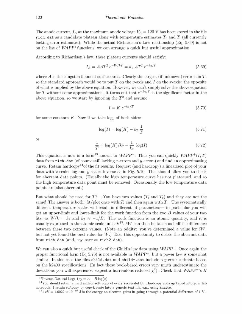
122 Thermionic Emission

The anode current, IA at the maximum anode voltage VA = 120 V has been stored in the filerich.dat as a candidate plateau along with temperature estimates Tr and Ti (all currentlylacking error estimates). While the actual Richardson’s Law relationship (Eq. 5.69) is noton the list of WAPP+functions, we can arrange a quick but useful approximation.

According to Richardson’s law, these plateau currents should satisfy:

IA = AAT 2 e−W/kT = k1 AT 2 e−k2/T (5.69)

where A is the tungsten filament surface area. Clearly the largest (if unknown) error is in T ,so the standard approach would be to put T on the y-axis and I on the x-axis: the oppositeof what is implied by the above equation. However, we can’t simply solve the above equationfor T without some approximations. It turns out that e−k2/T is the significant factor in theabove equation, so we start by ignoring the T 2 and assume:

I = K e−k2/T (5.70)

for some constant K. Now if we take loge of both sides:

log(I) = log(K)− k21

T(5.71)

or1

T= log(K)/k2 −

1

k2log(I) (5.72)

This equation is now in a form13 known to WAPP+. Thus you can quickly WAPP+(I, T )data from rich.dat (of course still lacking x-errors and y-errors) and find an approximatingcurve. Retain hardcopy14of the fit results. Request (and hardcopy) a linearized plot of yourdata with x-scale: log and y-scale: inverse as in Fig. 5.10. This should allow you to checkfor aberrant data points. (Usually the high temperature curve has not plateaued, and sothe high temperature data point must be removed. Occasionally the low temperature datapoints are also aberrant.)

But what should be used for T ?. . . You have two values (Ti and Tr) and they are not thesame! The answer is both: fit/plot once with Ti and then again with Tr. The systematicallydifferent temperature scales will result in different fit parameters— in particular you willget an upper-limit and lower-limit for the work function from the two B values of your twofits, as W/k = k2 and k2 ≈ −1/B. The work function is an atomic quantity, and it isusually expressed in the atomic scale unit eV15. δW can then be taken as half the differencebetween these two extreme values. (Note an oddity: you’ve determined a value for δW ,but not yet found the best value for W .) Take this opportunity to delete the aberrant datafrom rich.dat (and, say, save as rich2.dat).

We can also a quick but useful check of the Child’s law data using WAPP+. Once again theproper functional form (Eq 5.76) is not available in WAPP+, but a power law is somewhatsimilar. In this case the files child.dat and child-.dat include a y-error estimate basedon the k2400 specifications. (In fact these book-based errors very much underestimate thedeviations you will experience: expect a horrendous reduced χ2). Check that WAPP+’s B

13Inverse-Natural Log: 1/y = A+B log(x)14You should retain a hard and/or soft copy of every successful fit. Hardcopy ends up taped into your lab

notebook. I retain softcopy by copy&paste into a generic text file, e.g., using kwrite.151 eV = 1.6022 × 10−19 J is the energy an electron gains in going through a potential difference of 1 V.

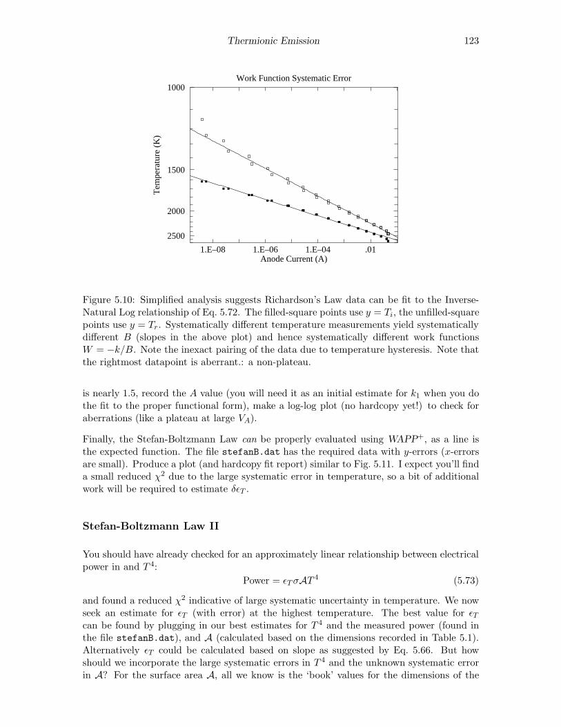
Thermionic Emission 123

1.E–08 1.E–06 1.E–04 .01

2500

2000

1500

1000Work Function Systematic Error

Anode Current (A)

Tem

pera

ture

(K

)

Figure 5.10: Simplified analysis suggests Richardson’s Law data can be fit to the Inverse-Natural Log relationship of Eq. 5.72. The filled-square points use y = Ti, the unfilled-squarepoints use y = Tr. Systematically different temperature measurements yield systematicallydifferent B (slopes in the above plot) and hence systematically different work functionsW = −k/B. Note the inexact pairing of the data due to temperature hysteresis. Note thatthe rightmost datapoint is aberrant.: a non-plateau.

is nearly 1.5, record the A value (you will need it as an initial estimate for k1 when you dothe fit to the proper functional form), make a log-log plot (no hardcopy yet!) to check foraberrations (like a plateau at large VA).

Finally, the Stefan-Boltzmann Law can be properly evaluated using WAPP+, as a line isthe expected function. The file stefanB.dat has the required data with y-errors (x-errorsare small). Produce a plot (and hardcopy fit report) similar to Fig. 5.11. I expect you’ll finda small reduced χ2 due to the large systematic error in temperature, so a bit of additionalwork will be required to estimate δǫT .

Stefan-Boltzmann Law II

You should have already checked for an approximately linear relationship between electricalpower in and T 4:

Power = ǫTσAT 4 (5.73)

and found a reduced χ2 indicative of large systematic uncertainty in temperature. We nowseek an estimate for ǫT (with error) at the highest temperature. The best value for ǫTcan be found by plugging in our best estimates for T 4 and the measured power (found inthe file stefanB.dat), and A (calculated based on the dimensions recorded in Table 5.1).Alternatively ǫT could be calculated based on slope as suggested by Eq. 5.66. But howshould we incorporate the large systematic errors in T 4 and the unknown systematic errorin A? For the surface area A, all we know is the ‘book’ values for the dimensions of the

124 Thermionic Emission

2 4 6 8 10

4.E+13

3.E+13

2.E+13

1.E+13

0

Stefan–Boltzmann Law

Power (W)

T^4

(K

^4)

Figure 5.11: A test of the Stefan-Boltzmann law: that power radiated is proportional toT 4. Note that the fit line hits well within each error bar. The χ2 for this fit will be“small”. Evidently the average temperature is a better measure of temperature than youmight expect from the deviations between Ti and Tr.

filament. Based on the sigfigs in the reported values, I estimate:

δAA ≈ 10% (5.74)

(mostly due to the filament diameter, where a ‘small’ uncertainty leads to a large fractionaluncertainty). We can then use the ‘high-low’ method or use the proper formula in AppendixE to estimate the range of possible values for ǫT , given the range of possible values for T 4

and A (assume the error in power is negligible).

Child’s Law II

At sufficiently high filament temperature (and low anode voltage), Child’s law governs theanode current-voltage relationship:

IA =8πǫ0ℓ

√

2em

9bβ2V

3

2

A (5.75)

(see vicinity of Eq. 5.40, page 109, for a definition of symbols) At the highest filamenttemperature (e.g., filament current of 2.4 A) you have saved the (VA, IA, δIA) data in thefile child.dat. Now fit16 this data to the functional form:

IA = k1 (VA − k2)3

2 (5.76)

16The program fit is documented in Appendix B. Note that plotting and fitting now are handled by twodifferent programs, not a combined program like WAPP

+

Thermionic Emission 125

1 10 100

.01

.001

.0001

Child’s Law

Va (V)

Ia (

A)

Figure 5.12: A plot of the space-charge limited thermionic emission in a FP-400 vacuumtube (Child’s law). The data was taken at a filament current of 2.4 A. Every other datapoint has been eliminated so the fit line is not obscured. Note that the fit line systematicallymisses the data, sometimes a bit high others a bit low. The measurement errors are tiny, sothese small misses do result in a “too-large” χ2. Nevertheless, the law provides an excellentsummary of the data over a huge range of variation.

(where k2 represents a small offset between ground and the actual average voltage of thefilament). The program fit will required an initial guess for k1; use the WAPP+value for Afound above. (In fit the default initial guess for parameters is zero; that is reasonable fork2.) Do not be surprised if you get a huge reduced χ2. Find an estimate for k1 error eitherby a ‘fudged fit’ or a bootstrap. As always retain a copy of your full fit report, including thecovariance matrix. Plot your data and best-fit function using the program plot, producinga result similar to Fig. 5.12.

Follow exactly the same process for the downsweep data in the file child-.dat. Often youwill find that the k1 values for the two sweeps differ by more than computer-based value ofδk1. Systematic error (here a type of hysteresis) is responsible. Note that the usual reducedχ2 alerts us to a problem, but measuring twice (in different ways) provides an estimate(perhaps still an under-estimate) for δk1: half the difference between the two values of k1.

We expect that

k1 =8πǫ0ℓ

√

2em

9bβ2(5.77)

so using the tube dimensions in Table 5.1, the electron charge-mass ratio e/m can becalculated. Since the FP-400 is a finite length cylinder (rather than the infinite cylinderdiscussed in our theory) use the effective length17 = 0.7 × ℓ as the length of the cylinder.

17This effective length corrects for current loss through the ends of the cylinder under space-charge sit-uations. A smaller correction should be applied when large anode voltages are designed to sweep up allevaporated electrons, i.e., for Richardson’s Law, where 90% electron collection seems appropriate. The

126 Thermionic Emission

160018002000220024002600

.01

.001

1.E–04

1.E–05

Richardson’s Law

Temperature (K)

Ano

de C

urre

nt (

A)

Figure 5.13: A Richardson Plot of thermionic emission in a FP-400 vacuum tube. Eachdata point displays the plateau anode current at a particular filament temperature. Thecurve through the data fits for the work function; the slightly steeper curve uses the bookvalue for the work function.

But what can we use as errors for the ‘book’ values for b and ℓ? Thermal expansion of thefilament should, by itself, change ℓ by about 1% (notice the spring-tensioned support forthe filament in the FP-400). Based on the sigfigs in the reported values, I estimate:

δ(b/ℓ)

(b/ℓ)≈ 3% (5.78)

Calculate e/m and its error. Compare to the ‘known’ value (citation required!).

Richardson-Dushman Law II

You should have already checked for an approximately exponential-inverse relationship be-tween T and IA, edited out aberrant data (e.g., not yet plateaued), and have a range ofpossible values (due to systematic error in temperature) for k2 in the expected relationship:

IA = k1 AT 2 e−k2/T (5.79)

We now seek a treatment incorporating the hysteresis error in IA and the proper functionalform, to obtain the best possible value for k2. We will need to manipulate18 the data inrich2.dat to bring together equivalent data from the temperature upsweep and downsweep.An easy way to get the data into the gnumeric spreadsheet, is to type it to the screen usingthe linux command19 cat:

details of handling such corrections to theory may be found in reference 1.18This processing could very easily have been done within the program itself. I’ve instead opted to make

the program as simple as possible at a cost of additional ‘by-hand’ processing in a spreadsheet.19from concatenate—commonly this command is used to combine several files

Thermionic Emission 127

cat rich2.dat

You can then copy and paste20 this data into gnumeric. Our aim to put together data withthe same filament current, i.e., to combine the first line of data with the last; to combinethe second line of data with the next-to-last; etc. This is easily accomplished by typing thedata bottom-to-top to the screen using the linux command21 tac:

tac rich2.dat

The results can be copy and pasted next to the previous data so that the data we aim tocombine (e.g., both If = 1 A) is on the same line. The best estimate for T is the average ofthe four T s (the two Ti should be nearly identical); the best estimate for IA is the averageof the two IAs; for δIA use half the difference between the two values of IA (|IA1 − IA2|/2);for δT use half the difference between Tr and Ti (average the two differences). The resultof this ‘data reduction’ is half as many data points, but with a value for δIA based onhysteresis. (The alternative for δIA would be the meter manufacturer’s specifications, andwe know they are way to small from analysis of Child’s Law.)

Report the relative importance of hysteresis and calibration in temperature uncertaintydetermination. For If = 1.2 A record the difference between the two Tr due to hysteresisand the difference between Tr and Ti which is a temperature calibration uncertainty.

Copy and paste this reduced data into a new file, and fit it to Eq. 5.79. (As always retaina copy of the full fit report.) You should have an estimate for k2 from WAPP+; use thebook22 value for A, 0.72 × 106 A/m2K2, as an initial guess for k1. Produce a plot similarto Fig. 5.13; include lines both for your best fit and the ‘book’ values of k1 and k2.

The work function is an atomic quantity, and it is usually expressed in the atomic scaleunit eV23. Calculate the work function from your value of k2 in joules and eV and compareto the book20 value of 4.5 eV.

Since our temperatures are so uncertain, particularly at the low end, the best estimate forthe Richardson constant A comes from substituting the book value of the work function andthe plateau (T, IA) measurement for the highest valid filament temperature into Eq. 5.69.We can then estimate the systematic uncertainty in A by using the ‘high-low’ method of191 (A+ → I+, T−,A−).

Report Checklist

1. Write an introductory paragraph describing the basic physics behind this experiment.For example, why did higher cathode currents produce ever higher plateaus of anodecurrent? (This manual has many pages on these topics; your job is condense this intoa few sentences and no equations.)

2. Calculations (no errors) of room temperature RW . Measurements (4-wire ohmmeterand direct voltage/current) of Rmeasured at room temperature. Calculation of Rsupport.

20Note use of “See two two separators as one”: Alt-e21clever or what?22Blakemore, Solid State Physics231 eV = 1.6022 × 10−19 J is the energy an electron gains in going through a potential difference of 1 V.

128 Thermionic Emission

3. Observations of the light intensity and color as a function of filament temperature.

4. Data files and computer program: Leave them in your linux account. Print out a copyof your program, the file filament.dat, and the data you used to fit Richardson’sLaw; Tape them into your lab notebook. Document how your Richardson’s Law datawas calculated in your spreadsheet. (I would self-document the spreadsheet, thenFilePrint AreaSet Print Area to select just the relevant 4 columns, including theself-documentation of those columns, and then print.)

5. Plots similar to Figures 5.9, 5.13 (with fit curve Eq. 5.68 and also the Richardsonfunction using “book” values for k1 and k2), 5.12 (with fit curve Eq. 5.67), 5.11(with line Eq. 5.66) and 5.10 (two separate WAPP+plots one with Tr data and theother with Ti data). Note that Figure 5.9 is complex to produce. Use a file of Nplotcommands and feel free to talk to me about how to go about doing this. Carefullynote the use of log and inverse scales (which requires positive data—edit to achievethis!). Include a fit report for each fit curve.

6. Experimental values (with error range) for: W (in eV), A, e/m and ǫT .

7. Show the steps connecting Equations (5.28)–(5.30) to Equation (5.31). Show thatf = Aρα is a solution to (5.31) if and only if A and α are as reported in Equation(5.36). Substitute the ρ → 1 approximation (Eq. 5.35) into the differential equation(5.31). Show that while we do not have an exact solution to the differential equation,the singular parts (i.e., those that approach infinity as ρ→ 1) cancel.

8. Make a final results table, recording your numerical results from #6 (with properunits and sigfigs) adjacent to the corresponding ‘book’ values. Don’t forget to recordyour tube’s identifying letter!

Comment: Classical vs. Quantum

I said above that the presence of an ~ in Richardson’s constant shows that the process isgoverned by quantum mechanics. It is not quite so simple. The evaporation of water is notfundamentally different from that of electrons, while the former (due to the larger mass of awater molecule) is well-approximated by a classical calculation. Classical evaporation can becalculated much as quantum evaporation using the Maxwell-Boltzmann speed distributionand the number density (of water molecules) rather than the disguised version of this: Fermi

energy (E3

2

F ∝ number density). We can write the classical rate in terms of the quantumwith no ~ visible:

classical flux =4

3√π

[

EF

kT

]3

2

× quantum flux (5.80)

The different temperature dependence24 for the classical flux (T1

2 e−W/kT vs. T 2e−W/kT )cannot be detected experimentally: the Boltzmann factor overwhelms all other temperaturedependencies. On the other hand, since EF ≫ kT , the expected classical rate is much largerthan the quantum rate. This played a role in the mistaken idea that thermionic emission

24Saul Dushman ( Phys. Rev. 21, 623–636 (1923)), while working at G.E., provided a general thermody-namic argument for the T 2 dependence and the universal nature of A. The resulting relationship is thereforesometimes known as the Richardson-Dushman relationship.

Thermionic Emission 129

was due to surface contamination: the experimental rate seemed too small to be thermalevaporation. On the other hand a more fruitful interpretation of the “low” rate was thatonly a fraction (∼ kT/EF ) of the electrons were thermally active. This connected withother observations (like the “small” specific heat of the electron gas) and provided a link tothe idea of a degenerate Fermi gas.

Comment: Uncertainty

Inspection of Figures 5.9-5.13 shows that something “funny” is going on. (I can’t say “ab-normal” or “unusual” as it is neither.) Figure 5.11 shows the unmistakable signs of “smallreduced χ2”: The fitted line goes nearly dead-center through all 30 error bars, never comingeven close to an edge. For error bars sized at one standard deviation (σ), you should expecttotal misses of the error bar about 1/3 of the time. In addition recall that each data pointis really a double: the same filament current was sourced as part of a temperature up-sweepand as part of a temperature down-sweep. These repeated measurement should also fre-quently miss by a standard deviation, but here they are so close that the two points oftenlook like just one. The answer to this puzzle is that the error bars are not displaying sta-tistical (‘random’) error. Instead the temperature was measured two different ways (Ti andTr), and the error bar represented the deviation between these two measurement methods.When different methods of measurement produce different answers for the same quantity,we have a textbook example of systematic error (in contrast to statistical error). Noticethat if we had used the statistical deviation of just one measure of temperature, we wouldseriously underestimated the error. Furthermore since quite accurately measured electricalquantities were used to calculate the temperature (via Equation 5.62 or Equation 5.56),application of the usual error propagation methods would also have produced very smallerrors in T . The full range of our uncertainty in temperature is made evident only bymeasuring T two different ways. (This is typically how systematic errors are detected.)

Having detected systematic errors, we should seek an explanation. . . In addition to theproblems previously cited (particularly use of book values for filament dimensions andthe problems associated with Rsupport), nonuniform filament temperature due to filamentsupports may be the problem. Koller (p. 89) reports the filament temperature 0.5 cm froma support is reduced by 15% (and of course the effect is greater closer to the support).Thermionic emission is reduced a similar amount 1.3 cm from a support. Thus the quantitywe are seeking (a filament temperature) does not even exist, so it is hardly surprising thatdifferent measurements give different results. (It turns out the Tr is something like theaverage temperature; whereas Ti is something like the central temperature.) These effectshave been investigated, and Koller gives the theory to correct such measurements, but suchconsiderations are beyond the scope of this experiment.

Figure 5.9 shows the opposite problem, “large reduced χ2”: The fitted line systematicallymisses almost every error bar. In this case, the miss might be called “small”, but the errorbar is smaller still. Once again, errors were not calculated statistically (manufacturer’sspecifications were used), so “reduced χ2 = 1” should not really be expected. In this case,my guess is that the problem is with our simplified theory (we assumed: infinite cylinders,no random component to the electron velocity [zero electron temperature], uniform filament[temperature, voltage, emissivity, . . . ], perfect vacuum, no incipient current plateau). Wecould of course test these hypotheses by further experiments with different tubes, but such

130 Thermionic Emission

work is beyond the scope of this experiment. (Indeed you most likely have detected VA-sweep hysteresis; correction for this dramatically reduces reduced χ2, but not all the wayto ∼ 1.)

Summary: Very large or very small reduced χ2 suggests significant non-statistical errors, avery common —perhaps even the usual— situation. Computer generated errors are somesort of none sense in this circumstance. Presumably your theory and/or measurementmethods are less than perfect. That is, of course, No Surprise. Science next requires youto guess and perhaps further investigate which imperfections are the leading source of theproblems, i.e., what changes to the experiment would ameliorate the problem.

References

1. Jones & Langmuir GE Review, The Characteristics of Tungsten Filaments as Func-tions of Temperature 30 (1927) Part I pp. 310–19, Part II pp. 354–61, Part III pp.408–12

2. Melissinos Experiments in Modern Physics, 1966, pp. 65–80

3. Preston & Dietz The Art of Experimental Physics, 1991, pp. 141–47, 152–61

4. Blakemore Solid State Physics, 1974, pp. 188–95

5. Koller The Physics of Electron Tubes, 1937, Ch. I, VI, VIII

6. G.E. FP-400 Description and Rating FP400.pdf found at http://www.tubedata.org

YESTERDAY IS HISTORYwords by Dr. James D. Livingstontune: Yesterday, by Paul McCartney

Yesterday — when old classical ideas held swayDrude and Maxwell-Boltzmann had their sayAnd we believed them yesterday

Suddenly — quantum free-electron theoryIntroduced the Fermi energyAnd yesterday was history

Fer-mi theory you’ll agree has much to sayWe see Drude was wrong — he belongs to yesterday

Density — of electron states provides the keyMultiplied by probabilityReveals electron propertiesYesterday is history

Thermionic Emission 131

thickness: ∆x

Area: A

x

E(x+∆x)

E(x)

∆x

Figure 5.14: Gauss’ Law is used to calculate the charge between two plates of area Aseparated by a distance ∆x. Since (by assumption) the potential just depends on x, theelectric field is in the x direction and is given by E = −dV/dx.

Appendix—Poisson’s Equation

Equation 5.5 and Equation 5.28 made reference to “Poisson’s Equation”, which is really atopic for Physics 341, rather than part of Physics 200. In this appendix, Poisson’s Equationis derived starting from two Physics 200 results: Gauss’ Law: that the electric flux leavinga region depends just on the charge enclosed by that region:

∮

~E · n dA = Qenclosed/ǫ0 (5.81)

and the relationship between electric field and electric potential (voltage):

Ex = − dV

dx(5.82)

Poisson’s Equation is a differential equation equivalent to Gauss’ Law. It is usually writtenin terms of the Laplacian (∇2), which in turn can most easily be expressed in terms ofsecond derivatives w.r.t. x, y, and z:

∇2V =∂2V

∂x2+∂2V

∂y2+∂2V

∂z2= −ρ/ǫ0 (5.83)

where ρ is the electric charge density. We need Poisson’s Equation only in cases wherethe electric potential depends on just one variable (x or cylindrical r), which simplifies therequired proofs considerably.

As shown in Figure 5.14, if V is a function of x alone: V (x), we can find the charge betweentwo plates of area A using Gauss’ Law:

Qenclosed = ǫ0A (E(x+∆x)− E(x)) ≈ ǫ0AdE

dx∆x (5.84)

Thus the charge density between the plates is given by:

ρ =Qenclosed

volume=ǫ0A dE

dx ∆x

A∆x= ǫ0

dE

dx= −ǫ0

d2V

dx2(5.85)

132 Thermionic Emission

l

r+∆r

thickness: ∆r

E(r+∆r)

E(r)

Figure 5.15: Gauss’ Law is used to calculate the charge between two coaxial cylinders oflength l separated by a distance ∆r. Since (by assumption) the potential just depends onr, the electric field is in the r direction and is given by E = −dV/dr.

which provides what is needed for Equation 5.5.

As shown in Figure 5.15, if V is a function of r alone: V (r), we can find the charge betweentwo coaxial cylinders using Gauss’ Law:

Qenclosed = ǫ0l 2π(r +∆r)E(r +∆r)− 2πrE(r)= ǫ0l 2πr(E(r +∆r)− E(r)) + 2π∆rE(r +∆r)

≈ ǫ0l

2πrdE

dr+ 2πE(r)

∆r (5.86)

Thus the charge density between the cylinders is given by:

ρ =Qenclosed

volume=ǫ0l 2πr dE/dr + 2πE(r)∆r

2πrl∆r= ǫ0

dE

dr+

1

rE

(5.87)

= − ǫ0

d2V

dr2+

1

r

dV

dr

(5.88)

which provides what is needed for Equation 5.28.

6: Scientific Paper

My freedom will be so much the greater and more meaningful the more nar-rowly I limit my field of action and the more I surround myself with obstacles.Whatever diminishes constraint, diminishes strength. The more constraints oneimposes, the more one frees one’s self of the chains that shackle the spirit. . . Andthe arbitrariness of the constraint serves only to obtain precision of execution

Igor StravinskyPoetics of Music in the Form of Six Lessons (1947) p.65

The devil is in the details

Anonymous

Paper Topics:

Presentation of a lab project as a scientific paper is the final component of this course. Iwill be assigning you a topic; feel free to drop me email with a list of your preferences!(First come, first served. Choose a topic ASAP and avoid the crunch at finals!) Topics:

1. Bubble Chamber: mµ

2. Bubble Chamber: mπ

3. Photometry: TB, TR

4. Thermionic Emission: Stefan-Boltzmann Law

5. Thermionic Emission: Richardson-Dushman Law

6. Thermionic Emission: Child-Langmuir Law

7. Langmuir Probe: Te

8. Langmuir Probe: ne

9. Langmuir Probe: Vf , Vp

133

134 Scientific Paper

Paper Basics:

sections: Title, Author(s) with affiliation, Abstract, Introduction, main body (tradi-tionally: Methods & Materials, Theory, Results, Discussion), Conclusions,Acknowledgments, References. You are encouraged to use specific (ratherthan the traditional generic) section titles in your main body.

first steps: Assemble your figures. Your figures should convey your main points: theyshould entice the expected audience to read a few words of the paper. Expectthat the reader will not read your paper: if at all possible, the figure captionsshould explain the figure to a skimming reader. Your figures must be legiblewhen reduced to a few inches; larger-than-normal fonts are usually required.Typically you will need to use a drawing program to make a block diagramof your apparatus.

Introduction: The Introduction explains why this experiment should be of interest to thereader. Cite and explain what other workers have discovered about the topic.(See these guys care about this stuff, so you should too!) Connect the exper-iment in the ongoing parade of science. Not uncommonly the experiment isof interest to you only because your Boss told you to do it. If so your Bossmay be able to transmit his enthusiasm for the project to you (or maybehe has some boilerplate you can recycle). Beware: the Introduction is theeasiest place to plagiarize (because it’s stuff all those people you cite alsowrote about). For me the Introduction is always the most interesting sectionto read: it starts with basic-level knowledge and brings me up-to-speed ona topic that I probably didn’t know much about to start.

Methods: Discussion of methods is often the hardest part to write. You know thethousand details the experiment required; now you must reduce that toa few paragraphs. If you’re lucky you can cite another paper for manydetails, but in any case you must inform the reader about what and howmeasurements were made; and how those meter readings related to deeperphysical concepts. You don’t need to tell the reader everything, but youmust say enough. In this lab paper you should report how you estimateduncertainties. Since these experiments often hinge on systematic error, youwill also discuss errors in sections discussing results. In most publishedpapers it is simply assumed that the errors have been properly estimated.Professionally the consequences for even accidental mis-estimation of errorscan be life-changing (non-tenure).

Abstract: While the Abstract is the first section of the paper, it is the last thingyou should write. The Abstract summarizes the significant items in thepaper including the results and conclusions. The Abstract should makesense isolated from the paper: do not refer to equations or figures in thepaper. (In fact collections of Abstracts are commonly separately publishedwithout the corresponding papers and are often the text digested by searchengines.) The Abstract should be short: perhaps a sentence for every section

Scientific Paper 135

of the paper. (The AIP Style Manual suggests the Abstract should be about5% of length of the article.)

Paper Shibboleths:

Gilead then cut Ephraim off from the fords of the Jordan, and whenever Ephraimitefugitives said, ‘Let me cross,’ the men of Gilead would ask, ‘Are you an Ephraimite?’If he said, ‘No,’ they then said, ‘Very well, say “Shibboleth” ’.(ש¤בלת!) If any-one said, “Sibboleth” ,(סבלת!) because he could not pronounce it, then theywould seize him and kill him by the fords of the Jordan. Forty-two thousandEphraimites fell on this occasion.

—Judges 12:5–6, NJB

My dictionary defines “shibboleth” as a peculiarity of speech that distinguishes a class ofpersons. I enlarge that definition here to mean a seemingly trivial peculiarity of usage thatresults in hugely disproportional results (death in the case of the Ephraimites). Scientificwriting has many constraints/details/shibboleths which must be followed in order to bepublished. (Hence a 65 page AIP Style Manual.)

In the opening quotes to this chapter, Maestro Stravinsky opines that constraints encouragecreativity and result in “precision of execution”; Anonymous suggests satanic torture inmeeting meaningless details. I believe at the end of this process you’ll most likely sidewith Anonymous. Oddly enough many of these writing details are designed to reduce youraudience: consistent information placement (for example in Abstract or Conclusions) allowsthe reader to read only what is immediately of interest (and perhaps skip your paper entirelyafter perusing your Abstract and Figures). Selective use of italics makes the mathematics(high information content) immediately obvious. True Maestros of scientific writing createwonderful scientific papers even with the constraints. I hope that your liberal arts educationhas helped you develop an effective, interesting writing style. However in this writingexercise, I’m going to be evaluating your attention to the stupid details required by (forexample) the AIP Style Manual. Frankly it would be asking too much to require you to getall these details right on this first try, so I outline below a small subset of critical formattingdetails that will affect your grade.

1. Proper formatting of mathematics: Letters standing for quantities (variables)are set in italics and are identified/defined in the text. (The names of compoundquantities, like vectors or matrices, may be set in a font distinct from that for simplequantities. For example, vectors are often set in bold.) Of course, non-letter mathglyphs: 1,2,+,=, . . . are set upright. Letters that are not variables (like “sin” in sin θor “max” in θmax) are also set upright. Many word processors have an “equationeditor” to make these font changes almost automatically. Equations that includemore than a few simple terms are “displayed”: isolated from the words on a new line.Displayed equations are numbered consecutively from the start of the document (orchapter in a book).

2. Proper formatting of figures: With the exception of actual photographs, figuresshould be “vector graphics”, like PostScript or SVG, not as pixel-based “raster graph-ics”, like jpeg or gif. Every figure includes a caption and is numbered consecutively

136 Scientific Paper

from the start of the document (or chapter in a book). Text in figures (for exampleaxis labels) must be legible even when the figure has been reduce to a few inches in size.The background of plots is blank (lacks the horizontal lines favored by spreadsheets).Generally figures “float” to the top or bottom of a page; they are not embedded withinthe body of the text. Figures you did not create yourself (e.g., copied from the web)include a credit to the actual creator.

3. Proper referencing: This is an example of “Do what I say, not what I did”. The“References” in this document are not in the proper form for a paper. (They areintended as a bibliography: sources that could be consulted for clarification or ex-pansion.) Every item in your References must be cited somewhere in the text. Theexact format of references/citations differs a between journals. There are two majorsystems: numbers in the text linked to numbered sources in References and (author,year) in the text with an alphabetical listing of sources in References. Professionallya program like BibTEX is usually used to manage both the basic reference databaseand the formatting of it in the style required by a specific journal. For this papersimply consistently use a reference format that will allow me to look up your refer-ences. Rule: You must cite at least two sources from peer reviewed journals/books.(You will probably additionally cite this lab manual, but it is not a peer reviewedjournal/book.) As I intend to actually look up your references, if a reference is notimmediately available to me (e.g., you received it via ILL or currently have the bookchecked out), include a copy of the reference with your paper.

4. Plagiarism: Detection of plagiarism is now trivial and an army of people enjoyouting famous authors for sins that would have gone undetected two decades ago.You must learn to avoid plagiarism, which I here define1 as 20 consecutive words 90%in common with published work. If you’re going to plagiarize, at least make detectingit an interesting challenge for me. For example, do not plagiarize this manual: Iwrote it and I remember what I wrote. It’s an interesting sporting question whetherto plagiarize from cited or non-cited works. Clearly its easier for me to check citedworks, but you then have the excuse that you weren’t seeking the original scientificcredit: a thief of words not discovery credit (misdemeanor not felony). If you arecaught plagiarizing from uncited works no excuse will save you. If you must exactlyreproduce the words of a published source, you must put those words in quotes,not just cite the source. Finally, note that trivial word substitutions do not solveplagiarism: you really must re-express the ideas in the source in your own words.Plagiarism: Again, recall that simple word changes do not eliminate plagiarism: youreally must express the concepts in the material in your own words.

5. Units, sigfigs, errors: The usual rules apply (see Lab Lint from 191). Essentiallyevery quantity in your paper will have units and an uncertainty. The uncertaintywill have no more than 2 significant digits. The place-value of the rightmost digit inquantity and error will match.

6. Draft Required! The course requires both a draft and a final-version of the paper.40% of the grade will be determined by your draft. Let me be clear about this: a draftis not an outline. If should be much the same length as the final paper; it should becomposed of English sentences. The figures and displayed equations in the draft maybe hand-drawn. The text of the draft should be complete (including, for example,

1FYI: online checkers like turnitin.com flag as potential plagiarism matches of 6 words.

Scientific Paper 137

figure captions). A draft is not a final version submitted twice. (The final versionmust respond to the comments I make in the draft.) If you do not submit a draft (e.g.,if you submit an outline or you submit nearly identical “drafts” and “final” papers)your maximum grade for the project will be 60%.

Important rules which you should follow (but which will not result in deductions).

1. Equations are part of sentences: Punctuation (comma, period) may be requiredby English usage at the end of displayed equations. Before the start of a new sentence,there should be a period from the previous sentence. (If you look carefully at thismanual, you’ll find I violate this rule when I think dots at the end of an equationmight cause confusion. Journals would not allow any exceptions.)

2. Proper formatting of tables: The AIP Style Manual has a full page of instructionsand many pages of examples on formatting tables. Frankly, following these rules isdifficult without a typesetting program like LATEX (which is briefly described below). Iwill mention one detail which surprised me when I was first informed of it: no verticallines in tables.

3. Special words: The AIP Style Manual has more than ten pages of preferred spellingsand abbreviations

TEX and LATEX

Because of the special formatting of scientific papers, most papers in math and physics aretoday typeset using the program LATEX. Most of the physics lab manuals and exams you’reseen have been written in LATEX. I love LATEX: I’ve been thinking of getting a “I♥TEX”bumper sticker or a photo of Don Knuth to put up in my office. But TEX really is bothdifficult to learn (it’s more like programming than writing) and stubborn and unyielding inaction. Only if you are thinking of going on to grad school in math or physics is it worthyour time to start to learn this beast. If you decide to give it a try, I promise to work withyou until you achieve the results desired.

In the on-line folder Examples+tex I’ve pulled a variety of papers from the web. The .pdfsin that folder show you the results; the subfolders show the “source” that produced thatoutput. If you’re not interested in TEX, view the .pdfs just to see what a scientific paperlooks like. As noted in files.txt John Dumm, Eric Garlid (Patton), and Ari Palczewskiwere 2005 SJU physics grads. Each is now closing in on a PhD (which typically requires pub-lishing some scientific papers) and I’ve pulled an example for each. Ross Terhaar suppliedme with the paper he wrote (in Word, I believe) for this course in 2010 (RossT2010.pdf).I converted his words into TEX to make the paper RossT2010rev.pdf. If you look at thedetails of these papers you’ll see minor differences in style, that reflect the required styleof the journal. (Examples: Figure 1 vs. FIG. 1; Table 2 vs. Table II; 6 Conclusions vs. VICONCLUSION; [Leybold Scientific, 2006a] vs. [2]) One of the nice things about TEX is thatminor changes to the documentclass can automatically change these formatting details ifyou decide to switch from, say, Phys.Rev. D to Ap.J.. Essentially all journals distinguishbetween preprint style (typically one column, double spaced: good for corrections) andreprint style (as it would appear in the journal, often two columns with smaller fonts).

138 Scientific Paper

References

1. Birgitta Malmfors, Phil Garnsworthy, and Michael Grossman Writing and PresentingScientific Papers (Nottingham Univ. Press, 2nd ed., 2003) T11.M34 2004 AlcuinReference

2. Robert A. Day How To Write & Publish a Scientific Paper (Oryx Press, 5th ed., 1998)T11 .D33 1998 Alcuin

3. Briscoe, Mary Helen Preparing Scientific Illustrations (Springer-Verlag, 1996) Q222.B751996 Alcuin

4. Jane Miller The Chicago Guide To Writing About Numbers (Univ. of Chicago Press,2004) T11.M485 2004 Alcuin Reference

5. Ivan Valiela, Doing Science: Design, Analysis, and Communication of Scientific Re-search (Oxford, 2nd ed., 2009) Q180.A1 V35 2001 Alcuin

6. http://www.physics.csbsju.edu/370/papers/links.html

7. Karin Knisely A Student Handbook for Writing in Biology (W.H. Freeman, 3rd ed.,2009) — more than a hundred pages on using Word/Excel for scientific writing; ILLonly

7: Langmuir’s Probe

Purpose

The purpose of this lab is to measure some basic properties of plasmas: electron tempera-ture, number density and plasma potential.

Introduction

When you think of electrical conductors, you probably think first of metals. In metals thevalence electrons are not bound to particular nuclei, rather they are free to move throughthe solid and thus conduct an electrical current. However, by far the most common electricalconductors in the Universe are plasmas: a term first applied to hot ionized gases by IrvingLangmuir (see below). In conditions rare on the surface of the Earth but common in theUniverse as a whole, “high” temperatures1 provide enough energy to eject electrons fromatoms. Thus a plasma consists of a gas of freely flying electrons, ions, and yet unionizedatoms. It should come as no surprise that during the extraordinary conditions of the BigBang, all the matter in the Universe was ionized. About 380,000 years after the Big Bang,the Universe cooled enough for the first atoms to form. Surprisingly about 400 million yearsafter that the Universe was re-ionized, and the vast majority of the matter in the universeremains ionized today (13.7 billion years after the Big Bang). Some of this ionized matteris at high density (hydrogen gas more dense than lead) and extremely high temperature atthe center of stars, but most of it is believed to be at extremely low density in the vastspaces between the galaxies.

Perhaps the most obvious characteristic of conductors (metals and plasmas) is that theyare shiny; that is, they reflect light. A moment’s thought should convince you that this is

1What does “high temperature” mean? When you are attempting to make a Bose condensation at lessthan a millionth of a degree, liquid helium at 4 K would be called hot. When you are calculating conditionsa few minutes after the Big Bang, a temperature of a billion degrees Kelvin would be called cool. Animportant insight: Nothing that has units can be said to be big or small! Things that have units need tobe compared to a “normal state” before they can be declared big or small. Here the normal state refers toconditions allowing normal solids and liquids to exist. Tungsten, which is commonly used in the filaments oflight bulbs, melts at about 3700 K; Carbon does a bit better: 3800 K. The “surface” of the Sun at 6000 Khas no solid bits. At temperatures of about 5000 K most molecules have decomposed into elements whichin turn have partially “ionized”: ejecting one or more electrons to leave a positively charged core (an ion)and free electrons. I’ll pick 5000 K as my comparison point for “hot”, but of course some elements (e.g.,sodium) begin to ionize a lower temperatures, and others (e.g., helium) ionize at higher temperatures. Thekey factor determining the ionized fraction in the Saha equation is the “first ionization energy”.

139

140 Langmuir’s Probe

not an “all-or-nothing” property. While metals reflect radio waves (see satellite TV dishes),microwaves (see the inside of your microwave) and visible light, they do not reflect higherfrequency light like X-rays (lead, not aluminum, for X-ray protection). The free electronnumber density (units: number of free electrons/m3), ne, determines the behavior of lightin a plasma. (Almost always plasmas are electrically neutral; i.e., the net electric chargedensity ρ is near zero. If the atoms are all singly ionized, we can conclude that the ionnumber density, ni, equals ne. In this lab we will be dealing with partially ionized argonwith a neutral atom density nn ≫ ne ≈ ni.) The free electron number density determinesthe plasma frequency, ωp:

ωp = 2πfp =

√

nee2

ǫ0m(7.1)

where −e is the charge on an electron and m is the mass of an electron. If light withfrequency f is aimed at a plasma: the light is reflected, if f < fp ; the light is transmit-ted, if f > fp. Thus conductors are shiny only to light at frequencies below the plasmafrequency. In order to reflect visible light, the plasma must be quite dense. Thus metals(ne ∼ 1028 m−3) look shiny, whereas semiconductors (ne ∼ 1024 m−3) do not. The plasmaat “surface” of the Sun (with ionized fraction less than 0.1% and ne ∼ 1020 m−3) wouldalso not look shiny. You will find the plasma used in this lab has even lower ne; it will looktransparent.

The defining characteristic of conductors (metals and plasmas) is that they can conduct anelectric current. Since conductors conduct, they are usually at a nearly constant potential(voltage). (If potential differences exist, the resulting electric field will automatically directcurrent flow to erase the charge imbalance giving rise to the potential difference.) Atfirst thought this combination (big current flow with nearly zero potential difference) maysound odd, but it is exactly what small resistance suggests. In fact the detection of bigcurrents (through the magnetic field produced) first lead to the suggestion2 of a conductorsurrounding the Earth—an ionosphere. Edward Appleton (1924) confirmed the existenceand location of this plasma layer by bouncing radio waves (supplied by a B.B.C. transmitter)off of it. In effect the ionosphere was the first object detected by radar. Appleton’s earlywork with radar is credited with allowing development of radar in England just in timefor the 1941 Battle of Britain. Appleton received the Nobel prize for his discovery of theionosphere in 1947. (Much the same work was completed in this country just a bit later byBreit & Tuve.)

The plasma frequency in the ionosphere is around 3–10 MHz (corresponding to ne ∼1011–1012 m−3). Thus AM radio (at 1 MHz) can bounce to great distances, whereas CBradio (at 27 MHz) and FM (at 100 MHz) are limited to line-of-sight. (And of coursewhen you look straight up you don’t see yourself reflected in the ionospheric mirror, asflight ∼ 5× 1014 Hz. On the other hand, extra terrestrials might listen to FM and TV, butwe don’t have to worry about them listening to AM radio.) The actual situation is a bitmore complex. In the lowest layer of the ionosphere (D region), the fractional ionizationis so low that AM radio is more absorbed than reflected. Sunlight powers the creation ofnew ions in the ionosphere, so when the Sun does down, ionization stops but recombinationcontinues. In neutral-oxygen-rich plasmas like the D region, the plasma disappears withoutsunlight. Higher up in the ionosphere (the F region, where ne is higher and nn lower) total

2Faraday (1832), Gauss (1839), Kelvin (1860) all had ideas along this line, but the hypothesis is usuallyidentified with the Scot Balfour Stewart (1882).

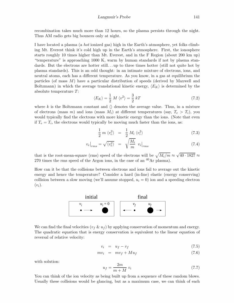
Langmuir’s Probe 141

recombination takes much more than 12 hours, so the plasma persists through the night.Thus AM radio gets big bounces only at night.

I have located a plasma (a hot ionized gas) high in the Earth’s atmosphere, yet folks climb-ing Mt. Everest think it’s cold high up in the Earth’s atmosphere. First, the ionospherestarts roughly 10 times higher than Mt. Everest, and in the F Region (about 200 km up)“temperature” is approaching 1000 K, warm by human standards if not by plasma stan-dards. But the electrons are hotter still. . . up to three times hotter (still not quite hot byplasma standards). This is an odd thought: in an intimate mixture of electrons, ions, andneutral atoms, each has a different temperature. As you know, in a gas at equilibrium theparticles (of mass M) have a particular distribution of speeds (derived by Maxwell andBoltzmann) in which the average translational kinetic energy, 〈EK〉 is determined by theabsolute temperature T :

〈EK〉 = 1

2M 〈v2〉 = 3

2kT (7.2)

where k is the Boltzmann constant and 〈〉 denotes the average value. Thus, in a mixtureof electrons (mass m) and ions (mass Mi) at different temperatures (say, Te > Ti), youwould typically find the electrons with more kinetic energy than the ions. (Note that evenif Te = Ti, the electrons would typically be moving much faster than the ions, as:

1

2m 〈v2e 〉 =

1

2Mi 〈v2i 〉 (7.3)

ve∣

∣

rms=√

〈v2e 〉 =

√

Mi

mvi∣

∣

rms(7.4)

that is the root-mean-square (rms) speed of the electrons will be√

Mi/m ≈√40 · 1827 ≈

270 times the rms speed of the Argon ions, in the case of an 40Ar plasma).

How can it be that the collisions between electrons and ions fail to average out the kineticenergy and hence the temperature? Consider a hard (in-line) elastic (energy conserving)collision between a slow moving (we’ll assume stopped, ui = 0) ion and a speeding electron(vi).

vi ui = 0

initialvf uf

final

We can find the final velocities (vf & uf ) by applying conservation of momentum and energy.The quadratic equation that is energy conservation is equivalent to the linear equation ofreversal of relative velocity:

vi = uf − vf (7.5)

mvi = mvf +Muf (7.6)

with solution:

uf =2m

m+Mvi (7.7)

You can think of the ion velocity as being built up from a sequence of these random blows.Usually these collisions would be glancing, but as a maximum case, we can think of each

142 Langmuir’s Probe

blow as adding a velocity of ∆u = 2mvi/(m+M) in a random direction. Consider the ionvelocity vector before and after one of these successive blows:

uf = ui +∆u (7.8)

u2f = u2i + (∆u)2 + 2 ui ·∆u (7.9)

Now on average the dot product term will be zero (i.e., no special direction for ∆u), so onaverage the speed-squared increases by (∆u)2 at each collision. Starting from rest, after Ncollisions we have:

u2f = N (∆u)2 (7.10)

1

2M u2f = N

1

2M (∆u)2 (7.11)

= N1

2M

[

2m

m+Mvi

]2

(7.12)

= N4m

m+M

M

m+M

1

2mv2i (7.13)

Thus for argon, N ≈ 18, 000 hard collisions are required for the ion kinetic energy to buildup to the electron kinetic energy. Note that in nearly equal mass collisions (e.g., betweenan argon ion and an argon atom), nearly 100% of the kinetic energy may be transferred inone collision. Thus ions and neutral atoms are in close thermal contact; and electrons arein close contact with each other. But there is only a slow energy transfer between electronsand ions/atoms. In photoionization, electrons receive most of the photon’s extra energy askinetic energy. Slow energy transfer from the fast moving electrons heats the ions/atoms.When the Sun goes down, the electrons cool to nearly the ion temperature.

Note that the hottest thing near you now is the glow-discharge plasma inside a fluorescentbulb: Te > 3× 104 K. . . hotter than the surface of the Sun, much hotter than the tungstenfilament of an incandescent light bulb. The cool surface of the bulb gives testimony to thelow plasma density (ne ∼ 1016–1017 m−3) inside the bulb. Containing this hot but rarefiedelectron gas heats the tube hardly at all — when the plasma’s heat gets distributed overhugely more particles in the glass envelope, you have a hugely reduced average energy, andhence temperature.

Plasma People

Irving Langmuir (1881–1957)

Born in Brooklyn, New York, Langmuir earned a B.S. (1903) in metallurgical engineeringfrom Columbia University. As was common in those days, he went to Europe for advancedtraining and completed a Ph.D. (1906) in physical chemistry under Nobel laureate WaltherNernst at University of Gottingen in Germany. Langmuir returned to this country, takingthe job of a college chemistry teacher at Stevens Institute in Hoboken, New Jersey. Dis-satisfied with teaching, he tried industrial research at the recently opened General ElectricResearch Laboratory3 in Schenectady, New York. Langmuir’s work for G.E. involved the

3G.E. calls this lab, which opened in 1900, the “first U.S. industrial laboratory devoted to research,innovation and technology”, but Edison’s Menlo Park “invention factory” (1876) would often claim thathonor. Bell Labs (founded 1925), with six Nobel prizes in physics, would probably claim to be the world’spreeminent industrial research lab, but the break up of the “Ma Bell” monopoly has also reduced Bell Labs.

Langmuir’s Probe 143

then fledgling4 electric power industry. He begin with improving the performance of incan-descent electric light bulb. (Langmuir is in the inventors hall of fame for patent number1,180,159: the modern gas-filled tungsten-filament incandescent electric light.) His workwith hot filaments naturally led to thermionic emission and improvements in the vacuumtriode tube that had been invented by Lee de Forest5 in 1906. Working with glow dischargetubes (think of a neon sign), he invented diagnostic tools like the Langmuir probe to in-vestigate the resulting “plasma” (a word he coined). “Langmuir waves” were discovered inthe plasma. Along the way he invented the mercury diffusion pump. In high vacuum, thinfilms can be adsorbed and studied. As he said in his 1932 Nobel prize lecture:

When I first began to work in 1909 in an industrial research laboratory, Ifound that the high-vacuum technique which had been developed in incandescentlamp factories, especially after the introduction of the tungsten filament lamp,was far more advanced than that which had been used in university laboratories.This new technique seemed to open up wonderful opportunities for the study ofchemical reactions on surfaces and of the physical properties of surfaces underwell-defined conditions.

In 1946, Langmuir developed the idea of cloud seeding, which brought him into contact withmeteorologist Bernard Vonnegut, brother of my favorite author Kurt Vonnegut. That’s howLangmuir became the model for Dr. Felix Hoenikker, creator of “ice-nine” in the novel Cat’sCradle. In fact Langmuir created the ice-nine idea (a super-stable form of solid water, withresulting high melting point, never seen in nature for want of a seed crystal) for H.G. Wellswho was visiting the G.E. lab.

Lyman Spitzer, Jr (1914–1997)

Lyman Spitzer was born in Toledo, Ohio, and completed his B.A. in physics from Yale in1935. For a year he studied with Sir Arthur Eddington at Cambridge, but that did notwork out so he returned to this country and entered Princeton. He completed his Ph.D. in1938 under Henry Norris Russell, the dean of American astrophysics. Following war workon sonar, he returned to astrophysics. His 1946 proposal for a large space telescope earnedhim the title “Father of the Hubble Space Telescope”.

Because of the bend in The Curve of Blinding Energy6, the lowest energy nuclei are ofmiddle mass (e.g., 56Fe). Thus nuclear energy can be released by breaking apart big nuclei(like 235Ur and 239Pu): fission as in the mis-named atomic bomb or by combining smallnuclei (like 2H deuterium and 3H tritium): fusion as in the hydrogen bomb. In 1943 EdwardTeller and Stanislaw Ulam started theoretical work on bombs based on thermonuclear fusionthen called “super” bombs. The end of WWII slowed all bomb work, but the explosion ofthe first Russian atomic bomb, “Joe 1”, in 1949, rekindled U.S. bomb work. This history ofrenewed interest in H-bomb work is mixed up with Russian espionage—real and imagined,

4Although not germane to my topic, I can’t resist mentioning the famous AC (with Tesla and Westing-house) vs. DC (with Edison, J.P. Morgan, and G.E.) power wars just before the turn of the century. Thebattle had a variety of bizarre twists, e.g., each side inventing an electric chair based on the opposite powersource aiming to prove that the opponent’s source was more dangerous than theirs. Easy voltage transfor-mation with AC guaranteed the victory we see today in every electrical outlet worldwide. Unfortunatelythe AC frequency did not get standardized so its 60 Hz here and 50 Hz in Europe.

51873–1961; “Father of Radio”, born Council Bluffs, Iowa, B.S & Ph.D. in engineering from Yale6Title of an interesting book by John McPhee; ISBN: 0374515980; UF767 .M215 1974

144 Langmuir’s Probe

“McCarthyism”, and the removal of Robert Oppenheimer’s7 security clearance in 1954.8

Our piece of the fusion story starts with Spitzer’s 1951 visit with John Wheeler9 in LosAlamos at just the right moment. The building of the Super, in response to Joe 1, had beenfailing: difficult calculations showed model designs would not ignite. Energy lost by thermalradiation and expansion cooled the “bomb” faster than nuclear energy was released.10 Butjust before Spitzer arrived, Ulam and Teller had come up with a new method (radiationcoupling for fuel compression) that Oppenheimer called “technically sweet”. Meanwhile, ina story Hollywood would love, Argentine president Juan Peron announced that his protege,Ronald Richter an Austrian-German chemist, working in a secret island laboratory hadachieved controlled fusion. The story (of course) fell apart in less than a year, but itgot both Spitzer and funding agencies interested. Spitzer’s idea (the “Stellarator”) was amagnetically confined plasma that would slowly fuse hydrogen to helium, releasing nuclearenergy to heat steam and turn electrical generators. Spitzer and Wheeler hatched a planto return to Princeton with a bit of both projects (of course funded by the government11):Project Matterhorn B would work on bombs and Project Matterhorn S would work onstellarators. Matterhorn B made calculations for the thermonuclear stage of the test shotMike (1 Nov 1952)—the first H-bomb. The device worked even better than they hadcalculated.

From 1951 until 1958 stellarator research was classified. Optimistic projections12 for fusionreactors were believed by all—after all physicists had completed key projects (atomic bomb,radar, H-bomb) like clockwork. Why should controlled fusion be much different from thecarefully calculated fusion of an H-bomb? Early hints of fusion success (neutron emission)turned out to be signs of failure: “instabilities” or disturbances that grew uncontrollablyin the plasma. Turbulence—the intractable problem in hydrodynamics13 from the 19th

century—came back to bite physics in the 1950s. Instead of the hoped-for “quiescent”plasma, experiment found large amplitude waves: a thrashing plasma that easily escapedthe magnetic field configurations physicists had thought should confine it. In 1961 Spitzerturned directorship of the Princeton Plasma Physics Laboratory (PPPL) over to MelvinGottlieb, and largely returned to astrophysical plasmas.

7J. Robert Oppenheimer (1904–1967): born New York, NY, Ph.D. (1927) Gottingen. Directed atomicbomb work at Los Alamos during WWII; ‘father of the atomic bomb’.

8See: Dark Sun, by Richard Rhodes, UG1282.A8 R46 19959John Archibald Wheeler (1911-2008): born Jacksonville, FL, B.S.+Ph.D. (1933) Johns Hopkins, Feyn-

man’s major professor at Princeton in 1942. Famous book: Gravitation. Coined the word “black hole”.10Curve of Binding Energy p. 64: One day, at a meeting of people who were working on the problem of

the fusion bomb, George Gamow placed a ball of cotton next to a piece of wood. He soaked the cotton withlighter fuel. He struck a match and ignited the cotton. It flashed and burned, a little fireball. The flamefailed completely to ignite the wood which looked just as it had before—unscorched, unaffected. Gamowpassed it around. It was petrified wood. He said, “That is where we are just now in the development of thehydrogen bomb.”

11The U.S. Atomic Energy Commission (AEC) initiated the program for magnetic fusion research underthe name Project Sherwood. In 1974 the AEC was disbanded and replaced by the Energy Research andDevelopment Administration (ERDA). In 1977, ERDA in turn was disbanded and its responsibilities trans-ferred to the new Department of Energy (DOE). Since 1977, DOE has managed the magnetic fusion researchprogram.

12An August 1954 report on a theoretical Model D Stellarator (only Model B, with a 2” tube, had actuallybeen built), using assumptions that proved false, projected a power output approximately four times thatof Hoover Dam. The usual joke is that controlled fusion will always be just ten years away.

13Turbulence in hydrodynamics is one of the Clay Millennium Prize Problems (essentially Nobel + Hilbertfor mathematics in this century): 1 million dollars for a solution!

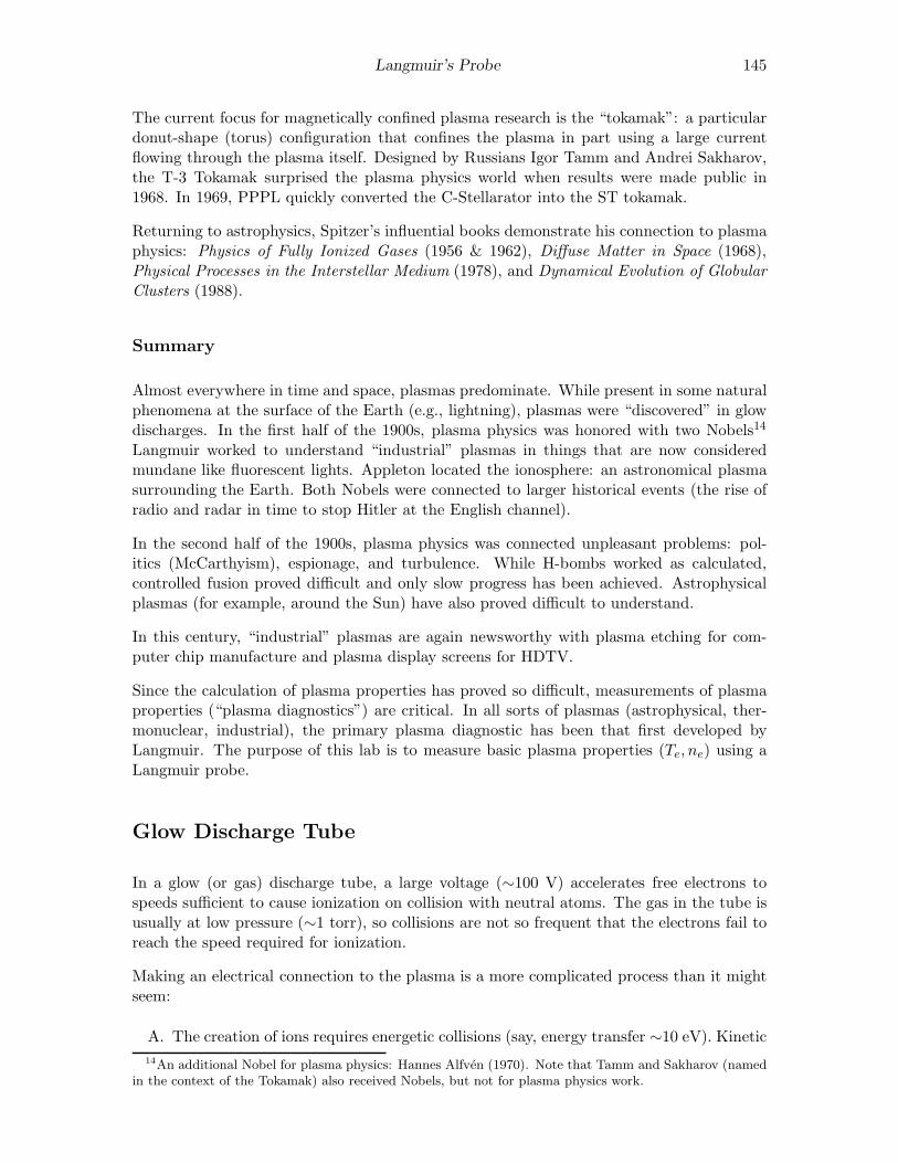
Langmuir’s Probe 145

The current focus for magnetically confined plasma research is the “tokamak”: a particulardonut-shape (torus) configuration that confines the plasma in part using a large currentflowing through the plasma itself. Designed by Russians Igor Tamm and Andrei Sakharov,the T-3 Tokamak surprised the plasma physics world when results were made public in1968. In 1969, PPPL quickly converted the C-Stellarator into the ST tokamak.

Returning to astrophysics, Spitzer’s influential books demonstrate his connection to plasmaphysics: Physics of Fully Ionized Gases (1956 & 1962), Diffuse Matter in Space (1968),Physical Processes in the Interstellar Medium (1978), and Dynamical Evolution of GlobularClusters (1988).

Summary

Almost everywhere in time and space, plasmas predominate. While present in some naturalphenomena at the surface of the Earth (e.g., lightning), plasmas were “discovered” in glowdischarges. In the first half of the 1900s, plasma physics was honored with two Nobels14

Langmuir worked to understand “industrial” plasmas in things that are now consideredmundane like fluorescent lights. Appleton located the ionosphere: an astronomical plasmasurrounding the Earth. Both Nobels were connected to larger historical events (the rise ofradio and radar in time to stop Hitler at the English channel).

In the second half of the 1900s, plasma physics was connected unpleasant problems: pol-itics (McCarthyism), espionage, and turbulence. While H-bombs worked as calculated,controlled fusion proved difficult and only slow progress has been achieved. Astrophysicalplasmas (for example, around the Sun) have also proved difficult to understand.

In this century, “industrial” plasmas are again newsworthy with plasma etching for com-puter chip manufacture and plasma display screens for HDTV.

Since the calculation of plasma properties has proved so difficult, measurements of plasmaproperties (“plasma diagnostics”) are critical. In all sorts of plasmas (astrophysical, ther-monuclear, industrial), the primary plasma diagnostic has been that first developed byLangmuir. The purpose of this lab is to measure basic plasma properties (Te, ne) using aLangmuir probe.

Glow Discharge Tube

In a glow (or gas) discharge tube, a large voltage (∼100 V) accelerates free electrons tospeeds sufficient to cause ionization on collision with neutral atoms. The gas in the tube isusually at low pressure (∼1 torr), so collisions are not so frequent that the electrons fail toreach the speed required for ionization.

Making an electrical connection to the plasma is a more complicated process than it mightseem:

A. The creation of ions requires energetic collisions (say, energy transfer ∼10 eV). Kinetic

14An additional Nobel for plasma physics: Hannes Alfven (1970). Note that Tamm and Sakharov (namedin the context of the Tokamak) also received Nobels, but not for plasma physics work.

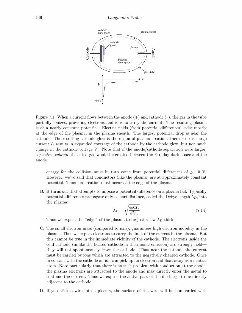
146 Langmuir’s Probe

Cat

hode A

node

plasma

plasma sheath

cathodeglow

cathodedark space

xV

−60 V

Faradaydark space

glass tube

Figure 7.1: When a current flows between the anode (+) and cathode (–), the gas in the tubepartially ionizes, providing electrons and ions to carry the current. The resulting plasmais at a nearly constant potential. Electric fields (from potential differences) exist mostlyat the edge of the plasma, in the plasma sheath. The largest potential drop is near thecathode. The resulting cathode glow is the region of plasma creation. Increased dischargecurrent Ic results in expanded coverage of the cathode by the cathode glow, but not muchchange in the cathode voltage Vc. Note that if the anode/cathode separation were larger,a positive column of excited gas would be created between the Faraday dark space and theanode.

energy for the collision must in turn come from potential differences of ∼> 10 V.However, we’ve said that conductors (like the plasma) are at approximately constantpotential. Thus ion creation must occur at the edge of the plasma.

B. It turns out that attempts to impose a potential difference on a plasma fail. Typicallypotential differences propagate only a short distance, called the Debye length λD, intothe plasma:

λD =

√

ǫ0kTee2ne

(7.14)

Thus we expect the “edge” of the plasma to be just a few λD thick.

C. The small electron mass (compared to ions), guarantees high electron mobility in theplasma. Thus we expect electrons to carry the bulk of the current in the plasma. Butthis cannot be true in the immediate vicinity of the cathode. The electrons inside thecold cathode (unlike the heated cathode in thermionic emission) are strongly held—they will not spontaneously leave the cathode. Thus near the cathode the currentmust be carried by ions which are attracted to the negatively charged cathode. Oncein contact with the cathode an ion can pick up an electron and float away as a neutralatom. Note particularly that there is no such problem with conduction at the anode:the plasma electrons are attracted to the anode and may directly enter the metal tocontinue the current. Thus we expect the active part of the discharge to be directlyadjacent to the cathode.

D. If you stick a wire into a plasma, the surface of the wire will be bombarded with

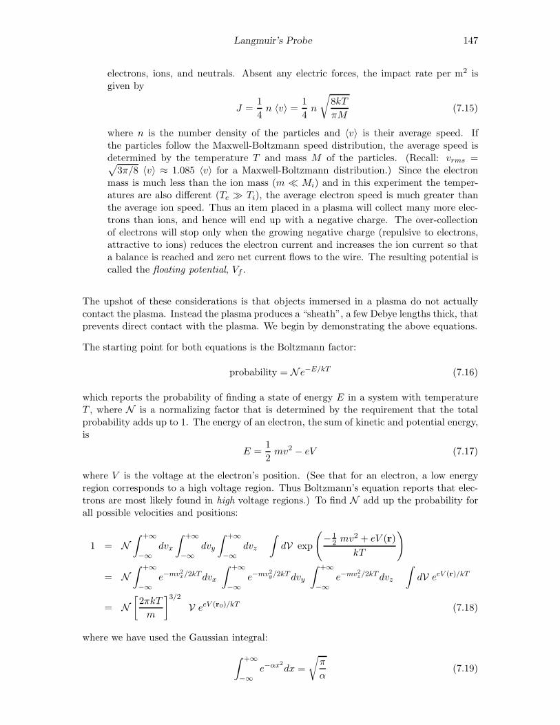
Langmuir’s Probe 147

electrons, ions, and neutrals. Absent any electric forces, the impact rate per m2 isgiven by

J =1

4n 〈v〉 = 1

4n

√

8kT

πM(7.15)

where n is the number density of the particles and 〈v〉 is their average speed. Ifthe particles follow the Maxwell-Boltzmann speed distribution, the average speed isdetermined by the temperature T and mass M of the particles. (Recall: vrms =√

3π/8 〈v〉 ≈ 1.085 〈v〉 for a Maxwell-Boltzmann distribution.) Since the electronmass is much less than the ion mass (m ≪ Mi) and in this experiment the temper-atures are also different (Te ≫ Ti), the average electron speed is much greater thanthe average ion speed. Thus an item placed in a plasma will collect many more elec-trons than ions, and hence will end up with a negative charge. The over-collectionof electrons will stop only when the growing negative charge (repulsive to electrons,attractive to ions) reduces the electron current and increases the ion current so thata balance is reached and zero net current flows to the wire. The resulting potential iscalled the floating potential, Vf .

The upshot of these considerations is that objects immersed in a plasma do not actuallycontact the plasma. Instead the plasma produces a “sheath”, a few Debye lengths thick, thatprevents direct contact with the plasma. We begin by demonstrating the above equations.

The starting point for both equations is the Boltzmann factor:

probability = N e−E/kT (7.16)

which reports the probability of finding a state of energy E in a system with temperatureT , where N is a normalizing factor that is determined by the requirement that the totalprobability adds up to 1. The energy of an electron, the sum of kinetic and potential energy,is

E =1

2mv2 − eV (7.17)

where V is the voltage at the electron’s position. (See that for an electron, a low energyregion corresponds to a high voltage region. Thus Boltzmann’s equation reports that elec-trons are most likely found in high voltage regions.) To find N add up the probability forall possible velocities and positions:

1 = N∫ +∞

−∞dvx

∫ +∞

−∞dvy

∫ +∞

−∞dvz

∫

dV exp

(

−12 mv

2 + eV (r)

kT

)

= N∫ +∞

−∞e−mv2x/2kTdvx

∫ +∞

−∞e−mv2y/2kTdvy

∫ +∞

−∞e−mv2z/2kTdvz

∫

dV eeV (r)/kT

= N[

2πkT

m

]3/2

V eeV (r0)/kT (7.18)

where we have used the Gaussian integral:

∫ +∞

−∞e−αx2

dx =

√

π

α(7.19)

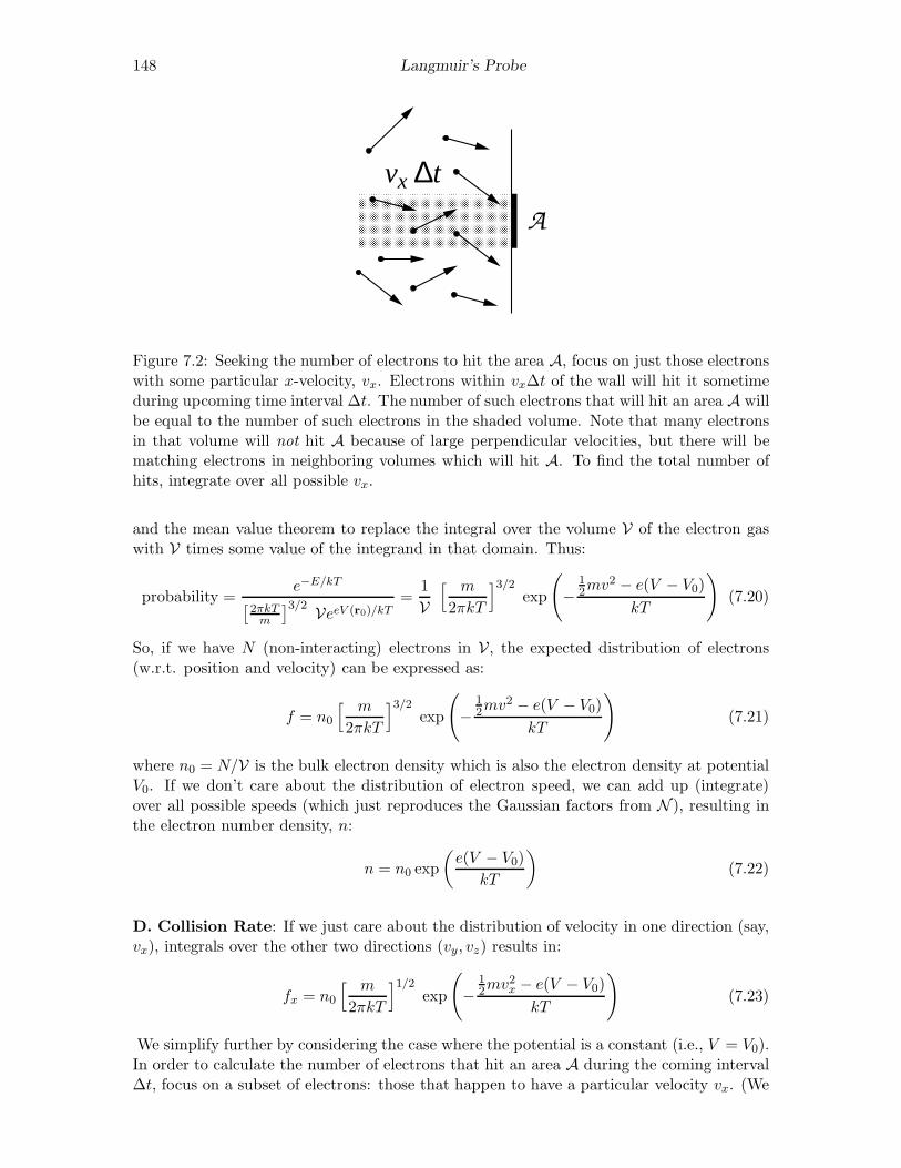
148 Langmuir’s Probe

A

CCCCCCCCCCCCCCCCCCCCCCCCCCCCCCCCCCCCCCCCCCCCCCCCCCCCCCCCCCCCCCCCCCCCCCCCCCCCCCCCCCCCCCCCCCCCCCCCCCCCCCCCCCCCCCCCCCCCCCCCCCCCCCCCCCCCCCCCCCCCCCCC

vx ∆t

Figure 7.2: Seeking the number of electrons to hit the area A, focus on just those electronswith some particular x-velocity, vx. Electrons within vx∆t of the wall will hit it sometimeduring upcoming time interval ∆t. The number of such electrons that will hit an area A willbe equal to the number of such electrons in the shaded volume. Note that many electronsin that volume will not hit A because of large perpendicular velocities, but there will bematching electrons in neighboring volumes which will hit A. To find the total number ofhits, integrate over all possible vx.

and the mean value theorem to replace the integral over the volume V of the electron gaswith V times some value of the integrand in that domain. Thus:

probability =e−E/kT

[

2πkTm

]3/2 VeeV (r0)/kT=

1

V[ m

2πkT

]3/2exp

(

−12mv

2 − e(V − V0)

kT

)

(7.20)

So, if we have N (non-interacting) electrons in V, the expected distribution of electrons(w.r.t. position and velocity) can be expressed as:

f = n0

[ m

2πkT

]3/2exp

(

−12mv

2 − e(V − V0)

kT

)

(7.21)

where n0 = N/V is the bulk electron density which is also the electron density at potentialV0. If we don’t care about the distribution of electron speed, we can add up (integrate)over all possible speeds (which just reproduces the Gaussian factors from N ), resulting inthe electron number density, n:

n = n0 exp

(

e(V − V0)

kT

)

(7.22)

D. Collision Rate: If we just care about the distribution of velocity in one direction (say,vx), integrals over the other two directions (vy, vz) results in:

fx = n0

[ m

2πkT

]1/2exp

(

−12mv

2x − e(V − V0)

kT

)

(7.23)

We simplify further by considering the case where the potential is a constant (i.e., V = V0).In order to calculate the number of electrons that hit an area A during the coming interval∆t, focus on a subset of electrons: those that happen to have a particular velocity vx. (We

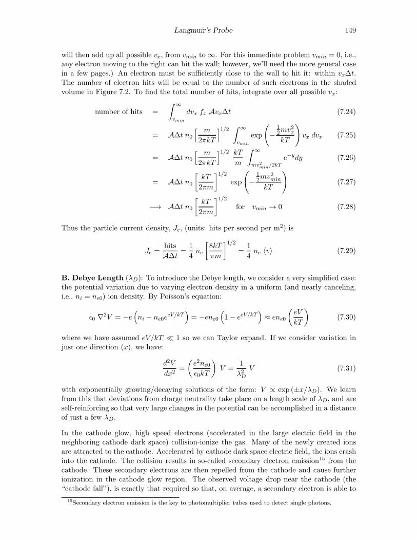
Langmuir’s Probe 149

will then add up all possible vx, from vmin to ∞. For this immediate problem vmin = 0, i.e.,any electron moving to the right can hit the wall; however, we’ll need the more general casein a few pages.) An electron must be sufficiently close to the wall to hit it: within vx∆t.The number of electron hits will be equal to the number of such electrons in the shadedvolume in Figure 7.2. To find the total number of hits, integrate over all possible vx:

number of hits =

∫ ∞

vmin

dvx fx Avx∆t (7.24)

= A∆t n0

[ m

2πkT

]1/2∫ ∞

vmin

exp

(

−12mv

2x

kT

)

vx dvx (7.25)

= A∆t n0

[ m

2πkT

]1/2 kT

m

∫ ∞

mv2min/2kTe−ydy (7.26)

= A∆t n0

[

kT

2πm

]1/2

exp

(

−12mv

2min

kT

)

(7.27)

−→ A∆t n0

[

kT

2πm

]1/2

for vmin → 0 (7.28)

Thus the particle current density, Je, (units: hits per second per m2) is

Je =hits

A∆t=

1

4ne

[

8kT

πm

]1/2

=1

4ne 〈v〉 (7.29)

B. Debye Length (λD): To introduce the Debye length, we consider a very simplified case:the potential variation due to varying electron density in a uniform (and nearly canceling,i.e., ni = ne0) ion density. By Poisson’s equation:

ǫ0 ∇2V = −e(

ni − ne0eeV/kT

)

= −ene0(

1− eeV/kT)

≈ ene0

(

eV

kT

)

(7.30)

where we have assumed eV/kT ≪ 1 so we can Taylor expand. If we consider variation injust one direction (x), we have:

d2V

dx2=

(

e2ne0ǫ0kT

)

V =1

λ2DV (7.31)

with exponentially growing/decaying solutions of the form: V ∝ exp (±x/λD). We learnfrom this that deviations from charge neutrality take place on a length scale of λD, and areself-reinforcing so that very large changes in the potential can be accomplished in a distanceof just a few λD.

In the cathode glow, high speed electrons (accelerated in the large electric field in theneighboring cathode dark space) collision-ionize the gas. Many of the newly created ionsare attracted to the cathode. Accelerated by cathode dark space electric field, the ions crashinto the cathode. The collision results in so-called secondary electron emission15 from thecathode. These secondary electrons are then repelled from the cathode and cause furtherionization in the cathode glow region. The observed voltage drop near the cathode (the“cathode fall”), is exactly that required so that, on average, a secondary electron is able to

15Secondary electron emission is the key to photomultiplier tubes used to detect single photons.

150 Langmuir’s Probe

Cat

hode A

node

plasma

glass tube

LangmuirProbe V, I power

supply

approx−60 V

plasma sheath

Voltage (V)

Cur

rent

(µA

)

0 2−2−4−6

0

20

40

60

80

100

−204 6

D C B A

floatingpotential

Vf

plasmapotential

Vp

Figure 7.3: At its simplest, a Langmuir probe is just a wire stuck into the plasma. Ofcourse, electrical contact with the plasma is limited by the plasma sheath. An externalpower supply allows the probe’s voltage to be adjusted and the resulting current measured.The characteristics of the plasma can be determined by careful analysis of the resulting IVrelationship.

reproduce itself through the above mechanism. Clearly the cathode fall depends both onthe gas (how easy it is to ionize) and the cathode material (how easy is it to eject secondaryelectrons). Luckily we will not need to understand in detail the processes maintainingthe discharge near the cathode. A properly operating Langmuir probe does not utilizesecondary electron emission, that is we limit voltage drop near the probe to much less thanthe cathode fall.

Langmuir Probe Theory

As stated above, if a wire is stuck into a plasma, instead of connecting to the plasmapotential (Vp) it instead charges to a negative potential (the floating potential: Vf < Vp)so as to retard the electron current enough so that it matches the ion current. An equalflow of electrons and ions—zero net current— is achieved and charging stops. If the wireis held at potentials above or below Vf , a net current will flow into the plasma (positive I:plasma electrons attracted to the probe), or out from the plasma (negative I: plasma ionsattracted to the probe). Figure 7.3 displays a Langmuir probe IV curve dividing it up intofour regions (A–D):

A. When the Langmuir probe is well above the plasma potential it begins to collect someof the discharge current, essentially replacing the anode.

B. When the probe is at the plasma potential (left side of region B), there is no plasmasheath, and the surface of the probe collects ions and electrons that hit it. The electroncurrent is much larger than the ion current, so at Vp the current is approximately:

Ip = eA1

4ne

[

8kTeπm

]1/2

(7.32)

Langmuir’s Probe 151

where A is the area of the probe. For V > Vp, the sheath forms, effectively expandingslightly the collecting area. Thus the probe current increases slightly and then levelsoff in this region.

C. When the Langmuir probe’s potential is below Vp, it begins to repel electrons. Onlyelectrons with sufficient kinetic energy can hit the probe. The minimum approachvelocity vmin allowing a probe hit can be determined using conservation of energy:

1

2mv2min − eVp = −eV (7.33)

1

2mv2min = e(Vp − V ) (7.34)

where the probe is at potential V . Equation 7.27 then reports that the resultingelectron current is

I = eA ne

[

kTe2πm

]1/2

exp

(

−e(Vp − V )

kTe

)

(7.35)

For V ≪ Vp, very few of the electrons have the required velocity. At V = Vf theelectron current has been suppressed so much that it equals the ion current. (The ioncurrent is always present in region C, but typically for V > Vf it is “negligible” incomparison to the electron current.)

D. In this region the probe is surrounded by a well developed sheath repelling all electrons.Ions that random-walk past the sheath boundary will be collected by the probe. Asthe sheath area is little affected by the probe voltage, the collected ion current isapproximately constant. (At very negative voltages, V ∼ −60 V, secondary electronemission following ion hits leads to large currents, and a glow discharge.) The equationfor this ion current is a bit surprising (that is not analogous to the seeming equivalentelectron current in region B):

Ii ≈ −1

2eA ni uB (7.36)

where uB is the Bohm16 velocity—a surprising combination of electron temperatureand ion mass:

uB =√

kTe/Mi (7.37)

Note that Equation 7.15 would have suggested a similar result but with the thermalvelocity rather than the Bohm velocity.

Region D: Ion Current

As shown in Figure 7.4, consider bulk plasma (ni = ne = n0, located at x = 0 with a plasmapotential we take to be zero Vp = 0) near a planar Langmuir probe (located at x = b biasedwith a negative voltage). In the bulk plasma, the ions are approaching the probe with a

16David Bohm (1917–1992) Born: Wiles-Barre, PA, B.S. (1939) PSU, joined Communist Party (1942),Ph.D. (1943) Berkeley — Oppenheimer’s last student before he became director at Los Alamos. Cited forcontempt by McCarthy’s House Un-American Activities Committee, Bohm was arrested in 1950. Althoughacquitted at trial, he was nevertheless blacklisted, and ended up in London.

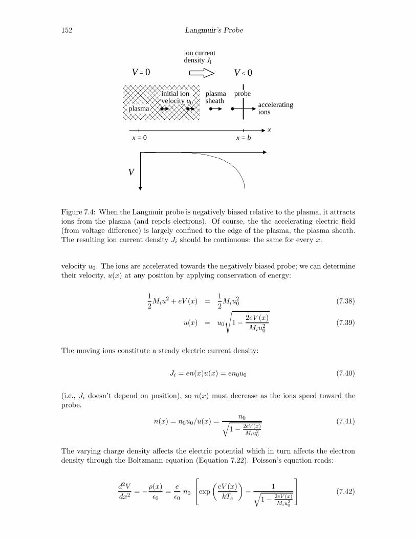
152 Langmuir’s Probe

plasmasheath

probe

xx = bx = 0

acceleratingions

ion currentdensity Ji

V = 0

&&&&&&&&&&&&&&&&&&&&&&&&&&&&&&&&&&&&&&&&&&&&&&&&&&&&&&&&&&&&&&&&&&&&&&&&&&&&&&&&&&&&&&&&&&&&&&&&&&&&&&&&&&&&&&&&&&&&&&&&&&&&&&&&&&&&&&&&&&&&&&&&&&&&&&&&&&&&&&&&&&&&&&&&&&&&&&&&&&&&&&&&&&&&&&

plasma

V

V < 0

initial ionvelocity u0

Figure 7.4: When the Langmuir probe is negatively biased relative to the plasma, it attractsions from the plasma (and repels electrons). Of course, the the accelerating electric field(from voltage difference) is largely confined to the edge of the plasma, the plasma sheath.The resulting ion current density Ji should be continuous: the same for every x.

velocity u0. The ions are accelerated towards the negatively biased probe; we can determinetheir velocity, u(x) at any position by applying conservation of energy:

1

2Miu

2 + eV (x) =1

2Miu

20 (7.38)

u(x) = u0

√

1− 2eV (x)

Miu20(7.39)

The moving ions constitute a steady electric current density:

Ji = en(x)u(x) = en0u0 (7.40)

(i.e., Ji doesn’t depend on position), so n(x) must decrease as the ions speed toward theprobe.

n(x) = n0u0/u(x) =n0

√

1− 2eV (x)Miu2

0

(7.41)

The varying charge density affects the electric potential which in turn affects the electrondensity through the Boltzmann equation (Equation 7.22). Poisson’s equation reads:

d2V

dx2= −ρ(x)

ǫ0=

e

ǫ0n0

exp

(

eV (x)

kTe

)

− 1√

1− 2eV (x)Miu2

0

(7.42)

Langmuir’s Probe 153

The first step in solving most any differential equation, is to convert it to dimensionlessform. We adopt dimensionless versions of voltage, position, and velocity:

V =eV

kTe(7.43)

x =x

λD= x

[

n0e2

ǫ0kTe

]1/2

(7.44)

u0 =u0uB

=u0

√

kTe/Mi

(7.45)

If we multiply Equation 7.42, by e/kTe, we find:

d2V

dx2=

1

λ2D

exp(V )− 1√

1− 2Vu20

(7.46)

ord2V

dx2= exp(V )− 1

√

1− 2Vu20

(7.47)

First let’s simplify notation, by dropping all those tildes.

d2V

dx2= exp(V )− 1

√

1− 2Vu20

(7.48)

The physical solution should show the neutral plasma picking up a positive charge densityas we approach the probe (as electrons are repelled and ions attracted to the probe). Ther.h.s. of Equation 7.48 is proportional to the charge density ne − ni which is nearly zero atx = 0 (where V = 0) and monotonically declines as x approaches the probe (where V < 0).If we Taylor expand the r.h.s., we find:

ne − ni ∝ exp(V )− 1√

1− 2Vu20

≈(

1 + V +1

2V 2 + · · ·

)

−(

1 +1

u20V +

3

2u40V 2 + · · ·

)

=

(

1− 1

u20

)

V +1

2

(

1− 3

u40

)

V 2 + · · · (7.49)

Thus u0 ≥ 1 is required for ni > ne when V < 0. Maximizing the extent of charge neutralityrequires u0 = 1. As shown in Figure 7.5, the choice u0 = 1 works throughout the V < 0range (i.e., beyond the range of convergence of the Taylor’s series).

Note that we can numerically solve this differential equation using Mathematica:

NDSolve[v’’[x]==Exp[v[x]]-1/Sqrt[1-2 v[x]/u0^2],v[0]==0,v’[0]==0,v,x,0,20]

but, it’s not quite that simple. The unique solution with these boundary conditions, isV = 0 everywhere. There must be some small electric field (V ′(0) < 0 ⇐⇒ E > 0) at x = 0due to probe. The smaller the choice of E, the more distant the probe. See Figure 7.6.

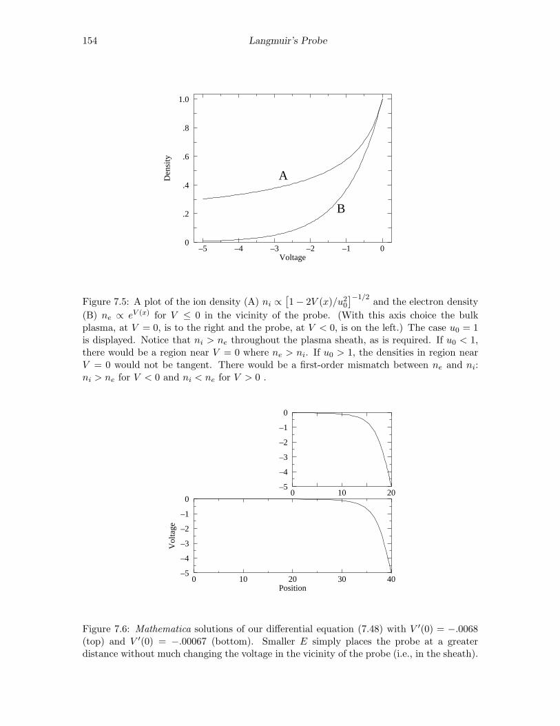
154 Langmuir’s Probe

–5 –4 –3 –2 –1 0

1.0

.8

.6

.4

.2

0

Voltage

Den

sity

A

B

Figure 7.5: A plot of the ion density (A) ni ∝[

1− 2V (x)/u20]−1/2

and the electron density

(B) ne ∝ eV (x) for V ≤ 0 in the vicinity of the probe. (With this axis choice the bulkplasma, at V = 0, is to the right and the probe, at V < 0, is on the left.) The case u0 = 1is displayed. Notice that ni > ne throughout the plasma sheath, as is required. If u0 < 1,there would be a region near V = 0 where ne > ni. If u0 > 1, the densities in region nearV = 0 would not be tangent. There would be a first-order mismatch between ne and ni:ni > ne for V < 0 and ni < ne for V > 0 .

0 10 20 30 40

0

–1

–2

–3

–4

–5

Position

Vol

tage

0 10 20

0

–1

–2

–3

–4

–5

Figure 7.6: Mathematica solutions of our differential equation (7.48) with V ′(0) = −.0068(top) and V ′(0) = −.00067 (bottom). Smaller E simply places the probe at a greaterdistance without much changing the voltage in the vicinity of the probe (i.e., in the sheath).

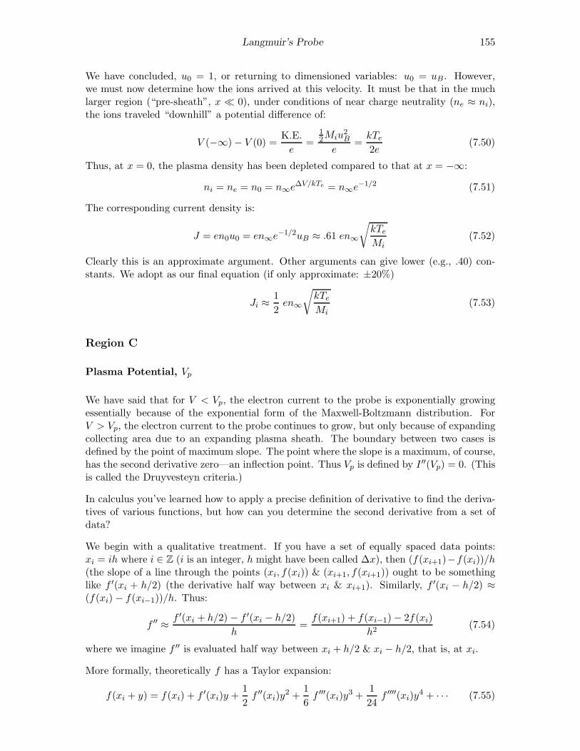
Langmuir’s Probe 155

We have concluded, u0 = 1, or returning to dimensioned variables: u0 = uB . However,we must now determine how the ions arrived at this velocity. It must be that in the muchlarger region (“pre-sheath”, x ≪ 0), under conditions of near charge neutrality (ne ≈ ni),the ions traveled “downhill” a potential difference of:

V (−∞)− V (0) =K.E.

e=

12Miu

2B

e=kTe2e

(7.50)

Thus, at x = 0, the plasma density has been depleted compared to that at x = −∞:

ni = ne = n0 = n∞e∆V/kTe = n∞e

−1/2 (7.51)

The corresponding current density is:

J = en0u0 = en∞e−1/2uB ≈ .61 en∞

√

kTeMi

(7.52)

Clearly this is an approximate argument. Other arguments can give lower (e.g., .40) con-stants. We adopt as our final equation (if only approximate: ±20%)

Ji ≈1

2en∞

√

kTeMi

(7.53)

Region C

Plasma Potential, Vp

We have said that for V < Vp, the electron current to the probe is exponentially growingessentially because of the exponential form of the Maxwell-Boltzmann distribution. ForV > Vp, the electron current to the probe continues to grow, but only because of expandingcollecting area due to an expanding plasma sheath. The boundary between two cases isdefined by the point of maximum slope. The point where the slope is a maximum, of course,has the second derivative zero—an inflection point. Thus Vp is defined by I ′′(Vp) = 0. (Thisis called the Druyvesteyn criteria.)

In calculus you’ve learned how to apply a precise definition of derivative to find the deriva-tives of various functions, but how can you determine the second derivative from a set ofdata?

We begin with a qualitative treatment. If you have a set of equally spaced data points:xi = ih where i ∈ Z (i is an integer, h might have been called ∆x), then (f(xi+1)−f(xi))/h(the slope of a line through the points (xi, f(xi)) & (xi+1, f(xi+1)) ought to be somethinglike f ′(xi + h/2) (the derivative half way between xi & xi+1). Similarly, f ′(xi − h/2) ≈(f(xi)− f(xi−1))/h. Thus:

f ′′ ≈ f ′(xi + h/2) − f ′(xi − h/2)

h=f(xi+1) + f(xi−1)− 2f(xi)

h2(7.54)

where we imagine f ′′ is evaluated half way between xi + h/2 & xi − h/2, that is, at xi.

More formally, theoretically f has a Taylor expansion:

f(xi + y) = f(xi) + f ′(xi)y +1

2f ′′(xi)y

2 +1

6f ′′′(xi)y

3 +1

24f ′′′′(xi)y

4 + · · · (7.55)

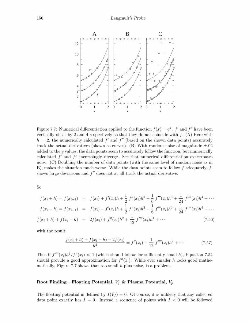
156 Langmuir’s Probe

0 1 2

12

10

8

6

4

2

A

0 1 2

B

0 1 2

C

ƒ

ƒ´´

ƒ´

x x x

Figure 7.7: Numerical differentiation applied to the function f(x) = ex. f ′ and f ′′ have beenvertically offset by 2 and 4 respectively so that they do not coincide with f . (A) Here withh = .2, the numerically calculated f ′ and f ′′ (based on the shown data points) accuratelytrack the actual derivatives (shown as curves). (B) With random noise of magnitude ±.02added to the y values, the data points seem to accurately follow the function, but numericallycalculated f ′ and f ′′ increasingly diverge. See that numerical differentiation exacerbatesnoise. (C) Doubling the number of data points (with the same level of random noise as inB), makes the situation much worse. While the data points seem to follow f adequately, f ′

shows large deviations and f ′′ does not at all track the actual derivative.

So:

f(xi + h) = f(xi+1) = f(xi) + f ′(xi)h+1

2f ′′(xi)h

2 +1

6f ′′′(xi)h

3 +1

24f ′′′′(xi)h

4 + · · ·

f(xi − h) = f(xi−1) = f(xi)− f ′(xi)h+1

2f ′′(xi)h

2 − 1

6f ′′′(xi)h

3 +1

24f ′′′′(xi)h

4 + · · ·

f(xi + h) + f(xi − h) = 2f(xi) + f ′′(xi)h2 +

1

12f ′′′′(xi)h

4 + · · · (7.56)

with the result:

f(xi + h) + f(xi − h)− 2f(xi)

h2= f ′′(xi) +

1

12f ′′′′(xi)h

2 + · · · (7.57)

Thus if f ′′′′(xi)h2/f ′′(xi) ≪ 1 (which should follow for sufficiently small h), Equation 7.54should provide a good approximation for f ′′(xi). While ever smaller h looks good mathe-matically, Figure 7.7 shows that too small h plus noise, is a problem.

Root Finding—Floating Potential, Vf & Plasma Potential, Vp

The floating potential is defined by I(Vf ) = 0. Of course, it is unlikely that any collecteddata point exactly has I = 0. Instead a sequence of points with I < 0 will be followed

Langmuir’s Probe 157

by points with I > 0, with Vf lying somewhere between two measured points. We seek tointerpolate to find the best estimate for Vf .

We begin with the generic case, where we seek a root, i.e., the x value such that y(x) = 0.We start with two data points (x1, y1) and (x2, y2) with y1 < 0 and y2 > 0. The lineconnecting these two points has equation:

y =∆y

∆x(x− x1) + y1 =

y2 − y1x2 − x1

(x− x1) + y1 (7.58)

We seek the x value for which the corresponding y value is zero:

∆y

∆x(x− x1) + y1 = y = 0 (7.59)

x− x1 = −y1∆x

∆y(7.60)

x = x1 − y1∆x

∆y(7.61)

In the case of the floating potential (I(Vf ) = 0), our (xi, yi) are a sequence of voltages withmeasured currents: xi = Vi, yi = I(Vi), and we can apply the above formula to find thevoltage, Vf where the current is zero.

The same generic result can be used to estimate the plasma potential, where I ′′(Vp) = 0.Here xi = Vi, yi = I ′′(Vi). Just as in the floating voltage case, it is unlikely that anycollected data point exactly has I ′′ = 0. Instead a sequence of points with I ′′ > 0 will befollowed by points with I ′′ < 0, with Vp lying somewhere between two measured points.You will apply the generic interpolate formula to find the best estimate for Vp.

Electron Temperature, Te

If we combine Equation 7.36 for the ion current with Equation 7.35 for the electron current,we have an estimate for the total current through out Region C:

I = −1

2eA ni uB +

1

4eA ne

[

8kTeπm

]1/2

exp

(

−e(Vp − V )

kTe

)

(7.62)

=1

2eA nuB

−1 +

[

2Mi

πm

]1/2

exp

(

−e(Vp − V )

kTe

)

(7.63)

= k1 + k2 exp ((V − Vp)/k3) (7.64)

Use of this equation is based on a long list of assumptions (e.g., constant collection area A,Maxwell-Boltzmann electron speed distribution, ni = ne = n. . . ). These assumptions arenot exactly true, so we do not expect this equation to be exactly satisfied: we are seeking asimplified model of reality not reality itself. By fitting this model equation to measured IVdata, we can estimate the parameters k1, k2, k3. Since k3 = kTe/e we can use it to estimatethe electron temperature. Similarly, k1 represents a measure of the ion current from which(once Te is known) ni can be calculated using Equation 7.36.

In order to start a non-linear fit as in Equation 7.64, we need initial estimates for theparameters ki. Measurement of Vf (where I = 0) and Equation 7.63, provide an estimate

158 Langmuir’s Probe

for Te:

0 = I =1

2eA n uB

−1 +

[

2Mi

πm

]1/2

exp

(

e(Vf − Vp)

kTe

)

(7.65)

1 =

[

2Mi

πm

]1/2

exp

(

e(Vf − Vp)

kTe

)

(7.66)

0 =1

2ln

[

2Mi

πm

]

−(

e(Vp − Vf )

kTe

)

(7.67)

e

kTe(Vp − Vf ) =

1

2ln

[

2Mi

πm

]

(7.68)

kTee

=2(Vp − Vf )

ln[

2Mi

πm

] (7.69)

Notice that the unit for k3 = kTe/e is volts, so ek3 = kTe in units of J or, most simply,k3 = kTe in units eV17 (since eV=e×Volt). It is common practice in plasma physics toreport “the temperature” [meaning kT ] in eV.

The ion current k1 can be estimated from the “saturated current” in Region D, i.e., thenearly constant current a volt or so below Vf . (For future convenience, we name this“saturated current” in Region D, Ii.)

See that for V = Vp, I = k1 + k2. Since the ion current is “negligible” for most of region C,we can estimate k2 from the measured current near Vp. (For future convenience, we namethe current actually measured at the data point just below Vp, Ip.)

Plasma Number Density, n

Given kTe, we have several of measuring n:

A. measured Ii and Equation 7.36, and

B. measured Ip and Equation 7.32,

Additionally we could use the fit values of Ii or Ip (k1 or k2, in Equation 7.64). Thesemethods will give answers that differ by a factor of 5 or more! When different ways ofmeasuring the same thing give different results, “systematic error” is the name of theproblem. The source of this problem is our imperfect model of current flow in RegionC (all those inaccurate assumptions). In particular, both (A) and (B) are hindered by theassumption of a Maxwell-Boltzmann speed distribution. (In fact measurements in Region Care commonly used tomeasure18 that speed distribution.) Often fit parameters are preferredto individual data points (essentially because the fit averages over several data points), butthat is not the case here. Thus the method considered most accurate is (A), although it

17Recall: 1 eV = 1.6022 × 10−19 J is the energy an electron gains in going through a potential differenceof 1 V.

18For example, Langmuir probes have been used to measure the electron speed distribution in the plasmathat gives rise to aurora (northern lights). The results show a non-Maxwellian speed distribution: lots ofhigh-speed “suprathermal” electrons.

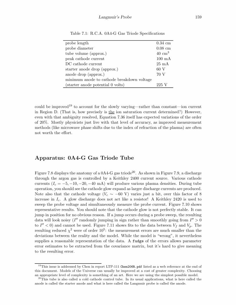
Langmuir’s Probe 159

Table 7.1: R.C.A. 0A4-G Gas Triode Specifications

probe length 0.34 cmprobe diameter 0.08 cmtube volume (approx.) 40 cm3

peak cathode current 100 mADC cathode current 25 mAstarter anode drop (approx.) 60 Vanode drop (approx.) 70 Vminimum anode to cathode breakdown voltage(starter anode potential 0 volts) 225 V

could be improved19 to account for the slowly varying—rather than constant—ion currentin Region D. (That is, how precisely is the ion saturation current determined?) However,even with that ambiguity resolved, Equation 7.36 itself has expected variations of the orderof 20%. Mostly physicists just live with that level of accuracy, as improved measurementmethods (like microwave phase shifts due to the index of refraction of the plasma) are oftennot worth the effort.

Apparatus: 0A4-G Gas Triode Tube

Figure 7.8 displays the anatomy of a 0A4-G gas triode20. As shown in Figure 7.9, a dischargethrough the argon gas is controlled by a Keithley 2400 current source. Various cathodecurrents (Ic = −5,−10,−20,−40 mA) will produce various plasma densities. During tubeoperation, you should see the cathode glow expand as larger discharge currents are produced.Note also that the cathode voltage (Vc ∼ −60 V) varies just a bit, over this factor of 8increase in Ic. A glow discharge does not act like a resistor! A Keithley 2420 is used tosweep the probe voltage and simultaneously measure the probe current. Figure 7.10 showsrepresentative results. You should note that the cathode glow is not perfectly stable. It canjump in position for no obvious reason. If a jump occurs during a probe sweep, the resultingdata will look noisy (I ′′ randomly jumping in sign rather than smoothly going from I ′′ > 0to I ′′ < 0) and cannot be used. Figure 7.11 shows fits to the data between Vf and Vp. Theresulting reduced χ2 were of order 105: the measurement errors are much smaller than thedeviations between the reality and the model. While the model is “wrong”, it neverthelesssupplies a reasonable representation of the data. A fudge of the errors allows parametererror estimates to be extracted from the covariance matrix, but it’s hard to give meaningto the resulting error.

19This issue is addressed by Chen in report LTP-111 Chen206R.pdf listed as a web reference at the end ofthis document. Models of the Universe can usually be improved at a cost of greater complexity. Choosingan appropriate level of complexity is something of an art. Here we are using the simplest possible model.

20This tube is also called a cold cathode control tube. In its usual applications, what is here called theanode is called the starter anode and what is here called the Langmuir probe is called the anode.

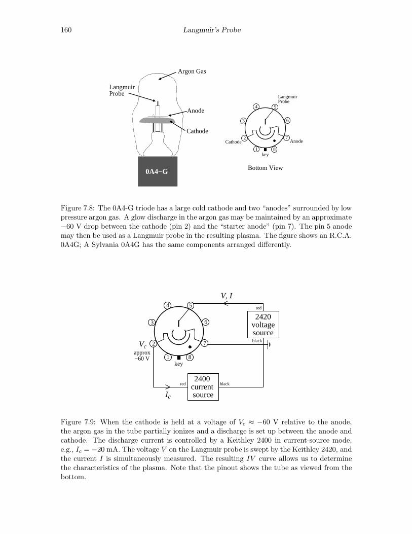
160 Langmuir’s Probe

Cathode

Anode

LangmuirProbe

Argon Gas

0A4−G

1

2

8

7

6

54

3

key

LangmuirProbe

Cathode Anode

Bottom View

Figure 7.8: The 0A4-G triode has a large cold cathode and two “anodes” surrounded by lowpressure argon gas. A glow discharge in the argon gas may be maintained by an approximate−60 V drop between the cathode (pin 2) and the “starter anode” (pin 7). The pin 5 anodemay then be used as a Langmuir probe in the resulting plasma. The figure shows an R.C.A.0A4G; A Sylvania 0A4G has the same components arranged differently.

1

2

8

7

6

54

3

key

2420voltagesource

2400current source

approx−60 V

Ic

Vc

V, I

red black

red

black

Figure 7.9: When the cathode is held at a voltage of Vc ≈ −60 V relative to the anode,the argon gas in the tube partially ionizes and a discharge is set up between the anode andcathode. The discharge current is controlled by a Keithley 2400 in current-source mode,e.g., Ic = −20 mA. The voltage V on the Langmuir probe is swept by the Keithley 2420, andthe current I is simultaneously measured. The resulting IV curve allows us to determinethe characteristics of the plasma. Note that the pinout shows the tube as viewed from thebottom.

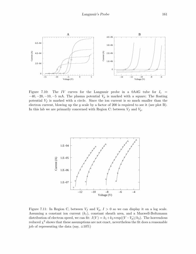
Langmuir’s Probe 161

–15 –10 –5 0 5

6.E–04

4.E–04

2.E–04

0

A

Voltage (V)

Cur

rent

(A

)

–14 –12 –10 –8 –6

4.E–06

3.E–06

2.E–06

1.E–06

0

B

Voltage (V)

Cur

rent

(A

)

Figure 7.10: The IV curves for the Langmuir probe in a 0A4G tube for Ic =−40,−20,−10,−5 mA. The plasma potential Vp is marked with a square; The floatingpotential Vf is marked with a circle. Since the ion current is so much smaller than theelectron current, blowing up the y scale by a factor of 200 is required to see it (see plot B).In this lab we are primarily concerned with Region C: between Vf and Vp.

–12 –10 –8 –6 –4

1.E–04

1.E–05

1.E–06

1.E–07

Voltage (V)

Cur

rent

(A

)

Figure 7.11: In Region C, between Vf and Vp, I > 0 so we can display it on a log scale.Assuming a constant ion current (k1), constant sheath area, and a Maxwell-Boltzmanndistribution of electron speed, we can fit: I(V ) = k1+k2∗exp((V −Vp)/k3). The horrendousreduced χ2 shows that these assumptions are not exact, nevertheless the fit does a reasonablejob of representing the data (say, ±10%)

162 Langmuir’s Probe

Computer Data Collection

As part of this experiment you will write a computer program to control the experiment.Plagiarism Warning : like all lab work, this program is to be your own work! Programsstrikingly similar to previous programs will alarm the grader. I understand that program-ming may be new (and difficult) experience for you. Please consult with me as you writethe program, and test the program (with tube disconnected!) before attempting a finaldata-collecting run.

In the following I’m assuming the probe voltage V is stored in array v(i), probe currentI is stored in array a(i), and the second derivative of prove current I ′′ is stored in arrayapp(i). Your program will control all aspects of data collection. In particular it will:

0. Declare and define all variables.

1. Open (i.e., create integer nicknames—i.e., iunit—for) the enets gpib1 and gpib2.

2. Initialize the source-meters which must be told the maximum voltage and current tooccur during the experiment. For the 2420, you can limit V, I to 25. V and .005 A;For the 2400, limit V, I to 100. V and 0.1 A;

3. Display the status of all devices before starting data collection.

4. Open files:

(a) VI.dump.dat (intended for all V, I, I ′′ of probe, with comments (!) for cathodeIc, Vc)

(b) VI.fit.dat (intended for Region C: V, I, δI, I ′′ of probe, with comments forcathode Ic, Vc, calculated Vf , Vp, estimated Te, measured Ii, Ip, and the numberof data points. The data points in this file are for fitting Equation 7.64:

f(x) = k1+ k2 ∗ exp((x− k4)/k3) (7.70)

Note that k4=Vp is a constant, not an adjustable parameter.)

5. Tell the 2400 source-meter to source a cathode current, Ic = −20 mA

6. Let the system sleep for 60 seconds to approach thermal equilibrium.

7. Repeat the below data collection process six times. Since you will need just threerepeats for each Ic, this will probably produce more data than is needed. Howeversome data sets may be noisy because of unstable (moving, flickering) cathode glow.Noisy data will have multiple sign changes in calculated I ′′; Discard this data. Ifone run of this program fails to produce enough good data (three repeats), simplyrename the data files (to preserve the data produced in the initial run), and re-runthe program.

Do the following for four different Ic: 5, 10, 20 40 mA (e.g., acath=-.005*2**j forj=0,3). Thus there will be 4× 6 voltage sweeps.

(a) Tell the 2400 source-meter to source a cathode current, Ic

(b) Let the system sleep for 10 seconds to approach thermal equilibrium.

Langmuir’s Probe 163

(c) Tell the 2420 to perform a linear probe voltage sweep from Vmin to Vmax, includ-ing N data points (say, N = 100). In Figure 7.10, you can see that the choicemade was Vmin = −15. and Vmax = +5., but your choices will vary and mustbe determined by trial and error (see below). The aim is to find a range thatincludes from a few volts below Region C to a few volts above Region C for everycathode current Ic.

(d) Turn off the probe voltage.

(e) Repeat (a) thus obtaining up-to-date values for Ic, Vc

(f) Write a comment (‘!’) line to the file VI.dump.dat containing Ic, Vc from the2400.

(g) Write a line to the file VI.dump.dat containing the first probe (V, I) data point:v(1), a(1)

(h) Do for i=2,N-1 the following:

i. Calculate I ′′ and store the value in the ith spot of an array i.e.,app(i)=a(i+1)+a(i-1)-2*a(i).

ii. Write the probe data: V, I, I ′′, i.e., v(i), a(i), app(i), to the file VI.dump.dat

(i) Write a line to the file: VI.dump.dat containing the last (i=N) data point V, I.

(j) Find the data point just before Vf with code21 like:

do i=2,N-1

if(a(i)>0.and.a(i+1)>0)goto 100

enddo

100 ivf=i-1

if(ivf.lt.15) STOP

The final line halts the program if ivf< 15, as we need Region D data to find theion current, Ii. If the program STOPs, Vmin will need to be reduced to capturethis data, and the program re-run.

(k) Using Equation 7.61 and the data points at ivf and ivf+1, find Vf . Note: in thegeneral case Equation 7.61, we were seeking x such that y(x) = 0; Here we areseeking Vf which is defined as the voltage such that I(Vf ) = 0, so, for example,x1 →v(ivf), y1 →a(ivf), and x→ Vf .

(l) Find the data point just before Vp with code22 like:

do i=ivf+1,N-2

if(app(i)<0.and.app(i+1)<0)goto 200

enddo

STOP

200 ivp=i-1

Note that the program is halted if the plasma potential has not been found beforewe run out of data. In that case Vmax will need to be increased to capture thisdata, and the program re-run.

21The check for two successive data points gone positive is done to avoid mistaking one point of noise forVf .

22The check for two successive data points with I ′′ < 0 is done to avoid mistaking one point of noise forVp

164 Langmuir’s Probe

(m) Using Equation 7.61 and the data points at ivp and ivp+1, find Vp. Note Vpis defined as the voltage such that I ′′(Vp) = 0, so, for example, x1 →v(ivp),y1 →app(ivp) , and x→ Vp.

(n) Write comment lines to the file: VI.fit.dat recording:

i. Ic, Vc, Vf , Vp (also print this to the screen, so you can monitor data collec-tion)

ii. ’!set k1= ’,a(ivf-15),’ k2= ’,a(ivp),’ k3= ’, 0.18615*(Vp − Vf )The aim here is to record basic plasma parameters (which are also neededas an initial guess in the fit to Equation 7.70) in a format that allows easycopy and paste into plot and fit. k1 is the measured ion current Ii; k2 isthe measured current at Vp (denoted Ip); k3 is an estimate for kTe/e, theelectron temperature in eV.Notes: The estimate for k3 is based on Equation 7.69 where 0.18615 =2/ ln(2Mi/πm). We are assuming that ivf-15 is far enough below Vf (i.e.,in Region D) that Ii = a(ivf− 15). You should check (after the fact) thatthis is the case, i.e., Vf − v(ivf− 15) ≫ k3. If this condition is not met,simply use a larger offset than 15 and re-run the program.

iii. ’!set k4= ’, Vp, ’ npoint= ’, ivp-ivf

k4 is the (not adjusted) plasma potential, Vp, whereas k1-k3 are varied fromthe above initial guesses to get the best fit to Equation 7.70 in Region C.

(o) For i=ivf+1,ivp write the probe data V, I, δI, I ′′ to the file VI.fit.dat withone V, I, δI, I ′′ data ‘point’ per line.

8. Turn off the output of the 2400.

9. Close all files.

Data Analysis

If all has gone well you have three good data sets for four different Ic, something like 1000data points. We could spend the next semester analyzing this data! Instead I suggest belowa simplified analysis scheme.

Start by making a composite plot similar to Figure 7.10A showing one IV curve for each ofthe four Ic. For these plots, choose Vmin & Vmax so that all behaviors (Regions A–D) aredisplayed. Make a similar plot showing three IV curves for one of the four Ic. The aim hereis to test for reproducibility; because of time limitations we’ll just check the reproducibilityof this one selected Ic. (I’ll call this selected Ic data set I∗c .) These six data sets (one IVcurve is on both plots) will be analyzed in greater detail. In order to properly fit the data,you will want to have more than 15 data points in the region between Vf and Vp (this mayrequire reducing the range Vmin through Vmax for the probe voltage sweep so it focuses juston Region C: say from about 4 V negative of the lowest Vf to 2 V positive of the highestVp and then re-taking the data). Additionally you should find that all six data sets haveapproximately the same number of data points.

Electron Temperature in eV: k3Fit Equation 7.70 to the six data sets. Note that the file itself contains the required initialguesses for adjusted parameters k1-k3 and the fixed value for k4. Expect to see large

Langmuir’s Probe 165

reduced χ2 which signals a too-simple model. No definite meaning can be attached to errorestimates from such poor fits, nevertheless some sort of nonsense needs to be reported.On page 16 we explored options for dealing with such ‘unusual’ fits. Option #5: ‘In direcircumstances’ you can use fudge command in fit to change your errors so that a reducedχ2 near one will be obtained. A re-fit with these enlarged errors then gives a new covariancematrix from which an estimate of parameter errors can be determined. Parameter valueswithin the range allowed by these errors would produce as good (or bad) a fit to the dataas the ‘best’ values. As the name suggests fudge is not exactly legitimate23 , neverthelessit is what Linfit has been silently doing all these years. Option #4: ‘Bootstrap’ the data:repeatedly fit subsets of the data and see how the resulting fit parameters vary with themultiple fits. This is essentially a way to repeat the experiment without taking new data.The fit command boots will report the results of nboot (default: 25) re-fits to subsets ofyour data along with the standard deviation of the fit parameters. Using either option, weare particularly interested in the some estimate of error in fit value of k3: use the squareroot of the appropriate diagonal element of the covariance matrix of a fudged fit or thereported standard deviation of k3 from a bootstrap.

For I∗c , compare the two errors for k3: σ (standard deviation of 3 fit values of k3) and thatfrom the fudged covariance matrix. Are they in the same ballpark (say, within a factor oftwo)?

Calculate the electron temperature of the plasma both in eV and K. Comment on therelationship (if any) between Te and Ic.

Plasma Number Density: nWe are interested in two sorts of ‘error’ in the plasma density n: reproducibility and anestimate of ‘systematic’ error. In the first case we’re asking: “given the same Ic is applied,how much do conditions in the plasma vary?” In the second case we interested in what theactual value of n is. We can estimate this systematic error by measuring n by two differentmethods:24 n calculated using Ii (Method A: let’s call this ni) and n calculated using Ip(Method B: let’s call this np). Let’s be clear here: ni, np, ne, n are all supposed to be thesame thing: the number of electrons (or ions) per m3 in the plasma. So

npni

=−Ip/Ii

√

2Mi/πm(7.71)

should be one; but it won’t be: systematic error is present!

In your lab notebook record these results in tables similar that shown in Table 7.225. (Forthis example, I selected I∗c = 20 mA.) Note particularly to record exactly the proper numberof significant figures in these tables! You should also copy & paste each full fit report into along concatenated file and include the resulting file in your notebook. As previously noted,the reduced χ2 for these fits is likely to be “horrendous”. Pick out your highest reduced χ2

fit, and plot the fitted function along with the data points on semi-log paper. (The resultsshould look similar to Figure 7.11, but with just one data set.) Do the same for the bestfit.

23for further discussion see: http://www.physics.csbsju.edu/stats/WAPP2 fit.html24See page 158; we are discussing here only methods A and B; methods using the fit parameters k1 and

k2 would be additional options.25The spreadsheet gnumeric may be of use.

166 Langmuir’s Probe

Table 7.2: Simplified data table for reporting Langmuir Probe results.

k3 Ic k3 fit σ(V) (mA) (V) error

40

20

105

Ii Ic median σ % error ni % error(A) (mA) Ii in Ii (m−3) in ni

40

20

10

5

Ip Ic median σ % error np/ni(A) (mA) Ip in Ip

40

20

10

5

Calculate26 n for each Ic based on the median Ii. Comment on the relationship (if any)between n and Ic. Make a power-law fit and log-log plot of the data27

Derive Equation 7.71. Calculate the np/ni and see that n has systematic error, i.e., ncalculated from Ip will be several times larger than the value of n calculated from Ii. Thisproves that there are problems with our simple theory.

Miscellaneous Calculations: ‘Lawson Product’ nτ , λD, fpIn 1957 J. D. Lawson determined that power generation from thermonuclear fusion requiredtemperature, plasma density n and the plasma confinement time τ to meet certain criteria:a temperature of at least 104 eV with the product: nτ > 1021 m−3 · s. We can estimate τbecause we know that our plasma is moving toward any surface at the Bohm velocity uB .Given that typically the plasma is within about 1 cm of a wall, find how long it remainsconfined, and calculate the “Lawson product” nτ for the I∗c plasma. (It is possible todirectly measure the plasma confinement time by using a scope to time the decay of theplasma when the glow discharge is suddenly turned off.)

Calculate the Debye length (λD, Eq. 7.14) and the plasma frequency (fp, Eq. 7.1) for I∗c .Compare λD to the diameter of the Langmuir probe. Will the sheath substantially expandthe collecting area A? According to Koller (p. 140, reporting the results of Compton &Langmuir28) the mean free path of an electron in a 1 torr argon gas is 0.45 mm. Compare

26http://www.physics.csbsju.edu/cgi-bin/twk/plasma.html can do this in one click.27I’d use WAPP+ : http://www.physics.csbsju.edu/stats/WAPP2.html.28Rev. Mod. Phys. 2 (1930) 208

Langmuir’s Probe 167

your λD to this electron mean free path.

Report Checklist

1. Write an introductory paragraph describing the basic physics behind this experiment.For example, why does the Langmuir probe current increase exponentially with probevoltage? Why is it that probe currents allow the calculation of plasma density? (Thismanual has many pages on these topics; your job is condense this into a few sentencesand no equations.)

2. Computer program: Print out a copy of your program and tape it into your labnotebook.

3. Plots:

(a) Similar to Figure 7.10A showing one IV curve for each of the four Ic.

(b) Similar to Figure 7.10A but showing three IV curves for I∗c .

(c) Two plots similar to Figure 7.11, showing the Region C fit to the data. (Theseplots are to display the best and worst reduced χ2; Record the reduced χ2 oneach plot.)

(d) Power law fit and log-log plot of four (Ic, n) data points.

4. Tabulated results from six fits for k3 (Te) at four different cathode currents includingfudged or bootstrapped results for δk3 and the standard deviation of three k3 for I∗c .You should copy & paste each full fit report into a long concatenated file. Print thatfile and tape it into your notebook. Record the identifying letter on your tube.

5. Tabulated results for measured Ii and Ip at four different cathode currents includingreproducibility errors estimated from the standard deviation.

6. Calculations (self-document spreadsheet or show sample calculations):

(a) kTe in units if eV for four Ic with estimates for errors.

(b) Te in units of K for four Ic.

(c) n calculated from median Ii and k3 for four Ic (with and estimate of reproducibil-ity error)

(d) np/ni calculated from median Ii and Ip (which provides an estimate of systematicerror)

(e) λD

(f) fp

(g) Lawson product at I∗c

7. Derivation of np/ni (Eq. 7.71).

8. Answers to the questions posed in the Data Analysis section:

(a) Are they in the same ballpark?

(b) Comment on the relationship (if any) between Te and Ic.

168 Langmuir’s Probe

(c) Comment on the relationship (if any) between n and Ic.

(d) Will the sheath substantially expand the collecting area A?

(e) Compare your λD to this electron mean free path.

9. Discussion of errors:

(a) Two methods were used to find “errors” in the electron temperature, Te: (A)fudged/bootstrap error from a fit and (B) σ from lack of reproducibility. Whatis the meaning and significance of fudged/bootstrap error? What is the meaningand significance of reproducibility error? How would you respond to the question:“What is the error in Te?” (Note a few sentences are required, not a number!)

(b) Two methods were used to find the plasma number density, n: methods basedon Ii and Ip. What is the meaning and significance of the fact that two differentways of measuring n produced different results. How would you respond to thequestion: “What is n?” (Note a few sentences are required, not a number!)

(c) Consider any one of the basic plasma parameters (n, Te, Vf , Vp) measured in thislab. Report any evidence that there is systematic error in the parameter. Reportyour best guess for the total error (systematic and random) in the parameter.Report how this error could be reduced.

Comment: Uncertainty

Area: Systemic Error

Both methods of calculating plasma density (ni and np) used the probe area A, which en-tered as an overall factor. The probe area was calculated based on the probe geometry datalisted in Table 7.1 which was supplied by reference #9 with no uncertainties. Clearly if theactual probe geometry differs from that in Table 7.1 there will be a systematic error in bothmethods of calculating n. If I guess the uncertainty in length and diameter measurementsbased on the number of supplied sigfigs, I find a 6% uncertainty in A. In 2008 a Sylvania0A4G tube was destroyed, and I took the opportunity to measure the the probe. The re-sults29 were quite different from those reported in Table 7.1: A was about 20% larger forthis Sylvania tube then for the RCA tube of reference #9. (The Sylvania/GE 0A4G alsolooks different from the RCA 0A4G.)

There is an additional significant problem: because the plasma sheath extends several λDbeyond the physical probe, there will be particle collection beyond the surface area of theprobe—the effective area is larger than the geometric surface area; we have made a SphericalCow by the simple assumption of A = πdℓ. A glace at Fig. 7.6 on page 154, shows thatthe plasma sheath extends about 10 × λD for ∆V ∼ 5 × kTe/e, which amounts to a largecorrection to probe diameter. Since the plasma sheath for ions30 in Region D has no reasonto be identical to the plasma sheath for electrons at the plasma potential, the effective Ain the two methods is probably not the same, and hence A does not really cancel out inderiving Eq. 7.71.

29diameter= 0.025”, length= .2”, the surrounding metal can is about 2 cm×3 cm.30For example, the mean free path for an electron is much larger than the mean free path for an ion

(approximately 4√2×).

Langmuir’s Probe 169

While we have lots of systematic and spherical cow error in our measurement of Te and n,it should also be emphasized that we do have ‘the right end of the stick’.

Interpreting Results

Inspection of Figure 7.11 shows the unmistakable signs of “large reduced χ2 ”: The fittedcurve misses many error bars. The miss might be called “small”, but the error bar issmaller still (in fact too small to show in this figure). The plasma density calculated fromIi disagrees with that calculated from Ip. What should be recorded as our uncertainty inTe and n? The problem is the result of using simplified theory. What can we conclude fromthe fits using inexact31 theory?

First the exponential IV relationship is clearly reflecting the Boltzmann factor at work. Tothe extent that there is an electron temperature, our k3 estimate must be fairly accurate.

On the other hand our n values disagree by a factor of three, and there are reasons tosuggest (e.g., uncertain A) the systematic error may be even larger. The disagreementbetween ni and np could be improved by better theory. (The assumed Maxwell-Boltzmannspeed distribution, collisions, varying collecting areas due to sheath expansion, . . . can becorrected —see particularly References 3 & 5.) However, for many practical purposes oneis interested in reproducible control rather measurement. One might be told that: “siliconwafer etching is to proceed when the indicated n reaches 1014 m−3” with no concern forwhat n actually is. Usually the reproducibility error found in the lab is only a few percent,which is often good enough for industrial control.

Of course, physics is most interested in reality, and what we have found is systematic error:two different ways of measuring n disagree. While one might argue that calculation of nbased on Ii is more robust than that based on Ip, fundamentally what is needed is additionalmethods of determining n to resolve the problem (see Reference 8). This is also beyond theaims of this lab. The best physics you can do based on this data is to report our estimatederrors with a clear warning that the systematic errors may be larger than the reporteduncertainty.

References

1. Maxwell & Benedict Theory of Gaseous Conduction and Electronics 1941 Chapter X

2. Koller Physics of Electron Tubes 1937 Chapter X

3. ed. Huddlestone & Leonard Plasma Diagnostic Techniques 1965 Chapter 4 by F. F.Chen Dewey 537.16028 H87

4. Chen Introduction to Plasma Physics and Controlled Fusion 1984 p. 295

5. ed. Auciello & Flamm Plasma Diagnostics 1989 Volume 1: Discharge Parameters andChemistry, Chapter 3 by N. Hershkowitz (ILL Madison)

6. Hutchinson Principles of Plasma Diagnostics 2001 Chapter 3 (ILL Bemidji)

31Note that all theory is inexact.

170 Langmuir’s Probe

7. http://www.physics.uiowa.edu/~fskiff/Physics_132/Lab%20Manual/B4Langmuir.PDF

8. http://www.ee.ucla.edu/~ffchen/Publs/Chen206R.pdf

9. I. Alexeff, J. T. Pytlinski, and N. L. Oleson Am. J. Phys. 45 (1977) 860–866, alsosee Am. J. Phys. 45 (1977) 1196–1199, Am. J. Phys. 46 (1978) 1276–1278, Am. J.Phys. 52 (1984) 753–754

Appendix A: fit

fit is a non-linear least-squares fitting program that allows you to fit (at most) nine param-eters of a function to data contained in a file. The function must be expressed as a singleline of intrinsic Fortran functions, real numbers, operations (+, -, *, /, ** or ^) and ad-justable parameters K1-K9. Both plot and fit use the prompt “*” to request commandsfor action from the user.

A typical fit session begins by using the editor to create a data file. When creating thedata file, follow this convention: reserve the first line of the file for an identifying sentence,and follow that line with columns of data separated by tabs or spaces. Typically you willput x values in the first column, y values in the second column, and y-errors (if available)in the third column. fit assumes this file is called fit.dat, but other filenames may beSET.

Once you have created the file, start the program by typing fit to the linux $ prompt:

$ fit

*

(At any time you may exit fit by holding down the Ctrl key and simultaneously hittingD. Note: the common windoze command Ctrl C kills programs rather than copies; simplyhighlight by sweeping with mouse and then hit the center mouse button to paste at thedesired location.) SET fit’s FILE variable equal to the filename of the file you just createdby typing:

* SET FILE=filename

If you have no y-errors (an unlikely situation!), inform the program by typing

* SET YECOL=0

(Don’t forget to hit the Return or Enter key after each line. Note: you cannot edit theselines using arrow keys: you must backspace!)

If any other columns are out of place, reSET fit’s other column location variables: XCOL

and YCOL. Note that fit will use no more than 512 data points. When fit is properlyinformed about your file type:

171

172 Appendix A: fit

* READ

and fit will read your data into its internal data storage area.

The next step is to tell fit the function you want it to fit to your data. As stated above,you must be able to express this function in one line using the intrinsic Fortran functions(e.g., log, log10, asin, ...), constant real numbers (e.g., 2, 6.03e23), operations (+,-, *, /, ** or ^), and (possibly) varying parameters (K1-K9). Examples:

* set f(x)=k1*exp(-((x-k2)/k3)**2)

* set f(x)=k1*(1-exp(k2*x))

* set f(x)=k1/sqrt((x-k2)^2+k3^2)

The function should be typed without using spaces. Note that the program automaticallytakes the absolute value of negative numbers raised to a power (e.g., (−2)3 = 8), but theSQRT of a negative number is zero. Use repeated multiplications to simulate integer powers(e.g., x3 = x ∗ x ∗ x), if the proper sign is required. Note that the default f(x) is thepolynomial k1+ k2 ∗ x+ k3 ∗ x2 + · · ·+ k9 ∗ x8, defined with repeated multiplication.

Now it’s time to SET your initial guess for the K parameters that occur in your function,with a command like:

* SET K1=3.14159 K2=4

Unlike linear least squares programs like WAPP+you must provide a moderately accurateinitial guess for each adjustable parameter. Time spent in careful consideration of parametervalues will be repaid many-fold. Bad initial parameter guesses will result in program crashes,long computer fit times, and inaccurate computer results. fit will step into the first chi-square (χ2) valley (χ2 minimum) it finds, and then stay there; so you must start fit close tothe right valley. It is advisable to try several different starting guesses for your parametersto find the path that leads to the lowest value of χ2.

Once you have a good initial guess for your K parameters, you may ask the computer toiterate to a minimum χ2. Of course, you must also tell the computer what K parameters itshould vary to find that minimum:

* fit

Enter list of Ks to vary, e.g. K1-K3,K5:

After you tell the computer what ks to vary, the machine will start its search. How doesfit know when to stop? It will, of course, never reach the exact valley bottom (i.e., χ2

minimum). If fit “finished” there is some evidence of convergence: either χ2 changedhardly at all during its last downward step (∆χ2=DELCHI, default=.1), or the parameters’first KSIG digits (default=4) didn’t change during its last downward step. Note: unchangingdigits for one step, should not be interpreted as unchanging digits for lots more steps, norshould it be interpreted as an error. If fit “quit” then it’s sick of trying (SET by NITER,

Appendix A: fit 173

default=100), so you should assume more steps are needed to reach the valley bottom. Thissuggests something is wrong. . . your initial guesses, the function, the data.

Once fit has quit or finished, it will print out summary results. Longer versions of theresults (including the covariance matrix needed to figure errors1) may be printed, typed onthe screen or placed in a file, at the users option. Always retain a copy of successful fitresults! Sometimes the found χ2 is so “bad” that you will be tempted to FUDGE, i.e., adjustyour y-errors until you get a reduced-χ2 of one. If you FUDGE be sure to write down whyyou think this cheating was justified.

A good way to estimate errors is to repeat the experiment lots of times. However very oftenthe required time is not available. fit provides a possibility legitimate way to simulateactual repeats: it repeatedly fits using random subsets of your data. This process is calledbootstrapping and it is invoked by the command BOOTST.

The command

* PRINT

will display your data (x, y, y-error, and f(x)) on the screen. fit will mark (?, !, :) pointsthat are 3, 2, or 1 y-errors away from f(x). Use this feature to see which data points arepoorly fit. Alternatively, you may use the program plot to display your data with fittedcurve.

You may find it helpful to do some parameter stepping yourself before you hand the finalfit over to fit. Put in a parameter guess, enter

* CHI

to find the resulting χ2, modify your guess and repeat the process.

fitting functions to data is an important and frustrating part of your education in physics.Good luck!

Report problems and/or suggestions to Tom Kirkman.

1If the reduced χ2 suggests a reasonable fit, the parameter uncertainties may be calculated from thesquare root of the corresponding diagonal element of the covariance matrix.

174 Appendix A: fit

Special Commands

Start—in a terminal type: fit$linux command — do any linux command from inside fit@filename — execute indirectly a file of fit commandsCtrl D — to exit programExamples:

* $ls *.dat

* @test.fit

fit Commands

(unambiguous abbreviations and lowercase allowed)

Syntax:

* COMMAND

* COMMAND VARIABLENAME = value, VARIABLENAME = value ...

Examples:

* SET K1=0, K2=1, K3=-1, F(X)=K1+K2*X**2+K3*X**4

* re yec=0, fi=expt.dat

BOOTST performs a bootstrap with NBOOT iterations

CHI calculates χ2 using F(X), Ks, and data.

FIT fits F(X) to your data (requests list of Ks to vary)

FUDGE destroys existing y-errors and renorms them so χ2 = NPOINT

HELP displays these messages

PRINT displays data stored in program and F(X) (marks large-deviation points)

READ reads data from FILE: see XCOL, YCOL, YECOL, ROW, IBEGIN, NPOINT, FILE

SET allows you to set variables values without doing any action

SHOW shows variable values

WRITE writes x, y, y-error, and f(x) to FILE

Appendix A: fit 175

fit Variables

A constant for use in F(X) (0)

B same(Note: A and B are used in WINDOW(X): WINDOW(X)=1 iff a ≤ x ≤ b, else zero)

C same

CHISQ most recent value of χ2 calculated

DELCHI fit stops if a step results in a χ2 change less than DELCHI (.1)

F(X) function use: A, ABS, ACOS, ASIN, ATAN, B, C, COS, COSH, EXP, INORM,

K, K1-K9, LOG, LOG10, NORM, PI, SIN, SINH, SQRT, TAN, TANH, WINDOW,

X, any real number, operations +, -, *, /, **, or ^

( K1+X*(K2+X*(K3+X*(K4+X*(K5+X*(K6+X*(K7+X*(K8+X*K9))))))) )

FILE READ/WRITEs data with this filename (fit.dat)

IBEGIN first array element used during CHI, FIT, READ, PRINT, WRITE (1)

K1-K9 possibly adjustable variables in F(X)

KSIG fit stops after a step if all Ks retain KSIG unchanged digits (4)

NBOOT number of bootstrap iterations performed (25)

NITER fit stops if more than NITER test steps are needed (100)

NPOINT number of points used during CHI, FIT, READ, PRINT, WRITE (512)

ROW first row of data in FILE (2)

SEED if negative, re-initializes random generator’s seed (-1)

XCOL column of x data in FILE — used during READ (1)

YCOL column of y data in FILE — used during READ (2)

YECOL column of y-error data in FILE — used during READ (3)Note: unread y-errors default to 1

176 Appendix A: fit

Appendix B: plot

plot is a general purpose, advanced plotting program. plot can be frustrating to usebecause it assumes you know what you want to do and actually mean what you say—so ifyou don’t know what you’re doing and don’t know what you say means to the machine, youcan draw a mess fast. Of course, after you know the program you should be able to drawa beautiful graph as fast as you drew that mess.

The most unusual feature of plot is the way you give values to the parameters needed todraw a graph, e.g., the size of the graph, maximum and minimum values, etc. Instead ofasking you if you want to change each of those 39 parameters, plot allows you to set themin any order, at any time you want. For example, if you want to change the minimum valueof x to 0, you type

* SET XMIN=0

(Don’t forget to hit the Return or Enter key after each line. Note: you cannot edit theselines using arrow keys: you must backspace!)

So the first thing you need to know is the name of the parameters. You will find a completelist at the end of this appendix but let me mention three important sets of parameters now.The first set determines the way the axes look: XMIN, XMAX, XSCALE and similarly for y.XMIN and XMAX should be self explanatory. XSCALE determines the nature of the scale:

XSCALE=1 is a linear (normal) scale;

XSCALE=2 is a logarithmic scale (distance in plot is proportional to log x);

XSCALE=3 is an inverse scale (distance in plot is proportional to 1x); and

XSCALE=4 is a probability scale (distance in plot is related to erf−1(x)).

(Note: you will rarely actually set XMIN and XMAX as there are autoscale commands, butyou will often be setting the type of scale.)

The second set determines how the program finds the proper data to plot. Basically to getnumbers (x, y, and errors) into the program you need to make a file with the editor. Thefirst line of this file should be a one-line description of the data in the file (i.e., free fall

experiment - trial #2). The following lines should consist of data—an x value, somespaces (or tabs or commas), the corresponding y value, some spaces, and the correspondingabsolute error in y. Thus when looked at as a whole, the first column will consist of xvalues, the second column the corresponding y values, etc. If you called this file plot.dat

177

178 Appendix B: plot

you have made a file exactly in the default manner. The program will be able to READ thisfile without telling it anything. If you put the x values in column 2, you will have to informthe program by typing

* SET XCOL=2

That is, XCOL is a variable that tells the program which column contains the x values.Similarly, YCOL, YECOL (y-error) and XECOL (x-error) are variable names. If you have noerrors, tell the program by typing

* SET YECOL=0

If you didn’t call your file plot.dat, you must tell the program by typing

* SET FILE=filename

Note the above SETing does not actually change the data inside the program. The datainside the program is only changed when you:

* READ

Finally the third set determines how functions are plotted.

* SET F(X)=SIN(PI*X)

* SET PMIN=-1 PMAX=1

* FCURVE

FCURVE will plot the function in the domain PMIN to PMAX (the “p” is for parameter—remember xmin and xmax have another meaning). Note that the border parameters (ymin,ymax, etc.) must be appropriately1 set before the function curve is added to the plot. F(X)can be set using the usual computer syntax2 for algebra. There are eleven built-in functionsthat correspond to the usual WAPP+ functions with the usual parameters A, B, and C.These can be plotted by SETting the function number NFUNCT to a value between 1 and 11.NFUNCT=0 (the default) plots the function F(X).

You use SET to tell the program on how you want your data displayed. To actually displaydata you need action commands. The sequence:

* READ

* SCALE

* BORDER

* DPOINT

1FSCALE will find appropriate ymin, ymax, etc., based on the function f(x) and domain PMIN to PMAX, butmore commonly the border parameters — including PMIN and PMAX — are set to fit the data with SCALE

2Note that you must use * for multiplication not just juxtaposition.

Appendix B: plot 179

tells the program to read the data (from the previously set FILE); SCALE tells the programto find appropriate XMIN, etc. given the data contained in the program; BORDER tells theprogram to display the graph outline you have described; DPOINT tells the program to plotthe data points. Type FCURVE to plot your function. Another useful command is HELP—ittypes out a listing of the commands and the variables.

Actually all this SETting and commanding can be done together as shown below: (note onecommand per line, but you may define several variables)

* READ YECOL=0, FILE=freefall1.dat

* SCALE

* BORDER TITLE=’Free Fall’, XLABEL=’Time (s)’, YLABEL=’Z (m)’

* DPOINT

* FCURVE PMIN=0, PMAX=.65, NFUNCT=10, A=0, B=0, C=4.9

Two final comments: The equal signs and commas in the above example make the readingof the line easier—but they make the typing of the line harder. You may substitute spacesfor them to make typing easier. Similarly, one gets tired of typing in the full command incapitals—lowercase and any unambiguous abbreviations may also be used. Thus instead ofthe above you may type:

* re yec 0 fi freefall1.dat

* sc

* bo tit ’FREE FALL’ xl ’TIME (s)’ yl ’Z (m)’

* dp

* fc pmin 0 pmax .65 nfu 10 a 0 b 0 c 4.9

Getting Hardcopy Plots

Now that you have a plot displayed on the terminal, you should want a copy of the screento put in your lab notebook. The command PCOPY will make a copy of the displayed plot tothe file specified by PFILE. If PFILE=" " (as it is by default), the output goes to the printer.

Special Commands

Start—in a terminal type: plot$linux command — do any linux command from inside plot@filename — execute indirectly a file of plot commandsCtrl D — to exit programExamples:

* $ls *.dat

* @fet.plt

Report problems/suggestions to Tom Kirkman.

180 Appendix B: plot

plot Commands

(unambiguous abbreviations and lowercase allowed)

Syntax:

* COMMAND

* COMMAND VARIABLENAME = value, VARIABLENAME = value ...

Examples:

* BORDER XMIN=0, XMAX=1, YMIN=-1, YMAX=1, TITLE=’now is the time’

* bo xmi 0 xma 1 ymi -1 yma 1 ti ’now is "the time"’

BORDER draws a border for a graph

CLEAR clears the screen

CROSSH digitizing mode—using the mouse move the ‘crosshair’ to the desired point. Holdthe Shift key and click; the x and y value at crosshair is reported.

DCURVE connects with a LINE NPOINT data points, starting with IBEGIN.

DPOINT plots NPOINT individual data points starting with IBEGIN; point symbol deter-mined by POINT, error bars by XECOL and YECOL

FCURVE plots the function NFUNCT for p from PMIN to PMAX in NSTEP steps. p = x forNFUNCTs 0–11, NFUNCT=0 displays F(X), link in funct(x,y,p,nfunct) for NFUNCT >11

FSCALE finds appropriate mins and maxs for x and y axes for FCURVE

HELP displays these messages

LABEL writes LABEL to the right of most recent CROSSHair

PCOPY copies plot to printer (lpr -Plp) or to PFILE

PRINTD displays data stored in program

READ reads data from FILE— see XCOL, YCOL, XECOL, YECOL, ROW, IBEGIN, NPOINT

SCALE finds appropriate min and max for x and y axes from NPOINT data pairs startingat IBEGIN (automatic 5% excess unless scale=0). Room for error bars included ifx & y ECOL not zero

SET allows you to set variables values without doing any action

SHOW shows variable values

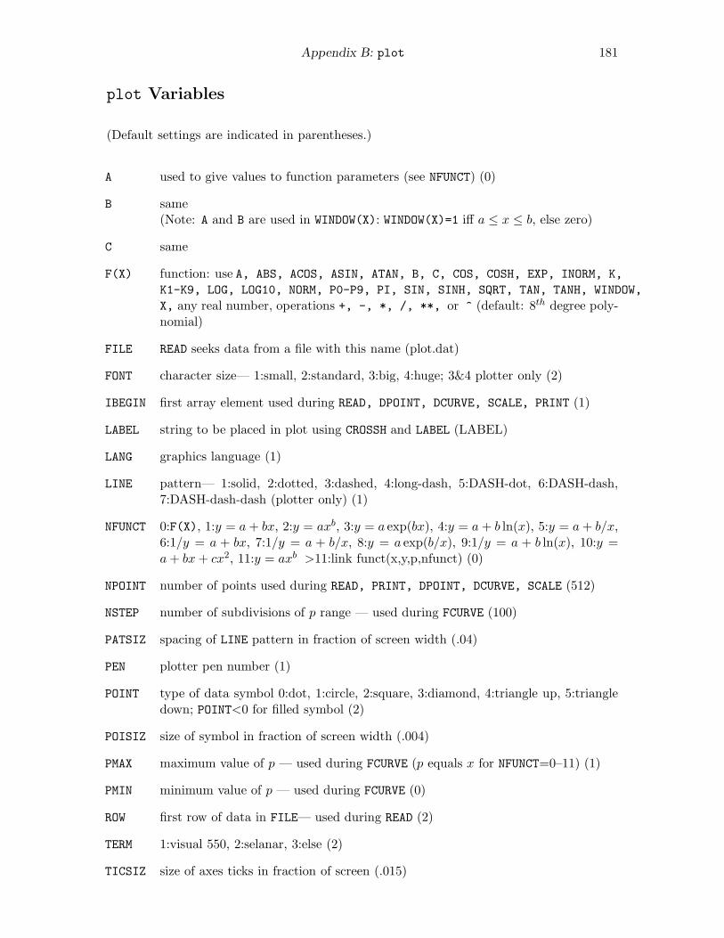
Appendix B: plot 181

plot Variables

(Default settings are indicated in parentheses.)

A used to give values to function parameters (see NFUNCT) (0)

B same(Note: A and B are used in WINDOW(X): WINDOW(X)=1 iff a ≤ x ≤ b, else zero)

C same

F(X) function: use A, ABS, ACOS, ASIN, ATAN, B, C, COS, COSH, EXP, INORM, K,

K1-K9, LOG, LOG10, NORM, P0-P9, PI, SIN, SINH, SQRT, TAN, TANH, WINDOW,

X, any real number, operations +, -, *, /, **, or ^ (default: 8th degree poly-nomial)

FILE READ seeks data from a file with this name (plot.dat)

FONT character size— 1:small, 2:standard, 3:big, 4:huge; 3&4 plotter only (2)

IBEGIN first array element used during READ, DPOINT, DCURVE, SCALE, PRINT (1)

LABEL string to be placed in plot using CROSSH and LABEL (LABEL)

LANG graphics language (1)

LINE pattern— 1:solid, 2:dotted, 3:dashed, 4:long-dash, 5:DASH-dot, 6:DASH-dash,7:DASH-dash-dash (plotter only) (1)

NFUNCT 0:F(X), 1:y = a+ bx, 2:y = axb, 3:y = a exp(bx), 4:y = a+ b ln(x), 5:y = a+ b/x,6:1/y = a + bx, 7:1/y = a + b/x, 8:y = a exp(b/x), 9:1/y = a + b ln(x), 10:y =a+ bx+ cx2, 11:y = axb >11:link funct(x,y,p,nfunct) (0)

NPOINT number of points used during READ, PRINT, DPOINT, DCURVE, SCALE (512)

NSTEP number of subdivisions of p range — used during FCURVE (100)

PATSIZ spacing of LINE pattern in fraction of screen width (.04)

PEN plotter pen number (1)

POINT type of data symbol 0:dot, 1:circle, 2:square, 3:diamond, 4:triangle up, 5:triangledown; POINT<0 for filled symbol (2)

POISIZ size of symbol in fraction of screen width (.004)

PMAX maximum value of p — used during FCURVE (p equals x for NFUNCT=0–11) (1)

PMIN minimum value of p — used during FCURVE (0)

ROW first row of data in FILE— used during READ (2)

TERM 1:visual 550, 2:selanar, 3:else (2)

TICSIZ size of axes ticks in fraction of screen (.015)

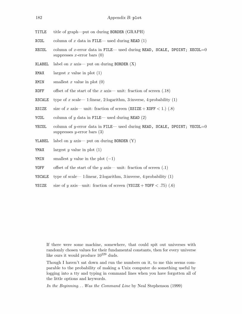
182 Appendix B: plot

TITLE title of graph—put on during BORDER (GRAPH)

XCOL column of x data in FILE— used during READ (1)

XECOL column of x-error data in FILE— used during READ, SCALE, DPOINT; XECOL=0suppresses x-error bars (0)

XLABEL label on x axis— put on during BORDER (X)

XMAX largest x value in plot (1)

XMIN smallest x value in plot (0)

XOFF offset of the start of the x axis— unit: fraction of screen (.18)

XSCALE type of x scale— 1:linear, 2:logarithm, 3:inverse, 4:probability (1)

XSIZE size of x axis— unit: fraction of screen (XSIZE+ XOFF < 1.) (.8)

YCOL column of y data in FILE— used during READ (2)

YECOL column of y-error data in FILE— used during READ, SCALE, DPOINT; YECOL=0suppresses y-error bars (3)

YLABEL label on y axis— put on during BORDER (Y)

YMAX largest y value in plot (1)

YMIN smallest y value in the plot (−1)

YOFF offset of the start of the y axis— unit: fraction of screen (.1)

YSCALE type of scale— 1:linear, 2:logarithm, 3:inverse, 4:probability (1)

YSIZE size of y axis—unit: fraction of screen (YSIZE+ YOFF < .75) (.6)

If there were some machine, somewhere, that could spit out universes withrandomly chosen values for their fundamental constants, then for every universelike ours it would produce 10229 duds.

Though I haven’t sat down and run the numbers on it, to me this seems com-parable to the probability of making a Unix computer do something useful bylogging into a tty and typing in command lines when you have forgotten all ofthe little options and keywords.

In the Beginning. . .Was the Command Line by Neal Stephenson (1999)

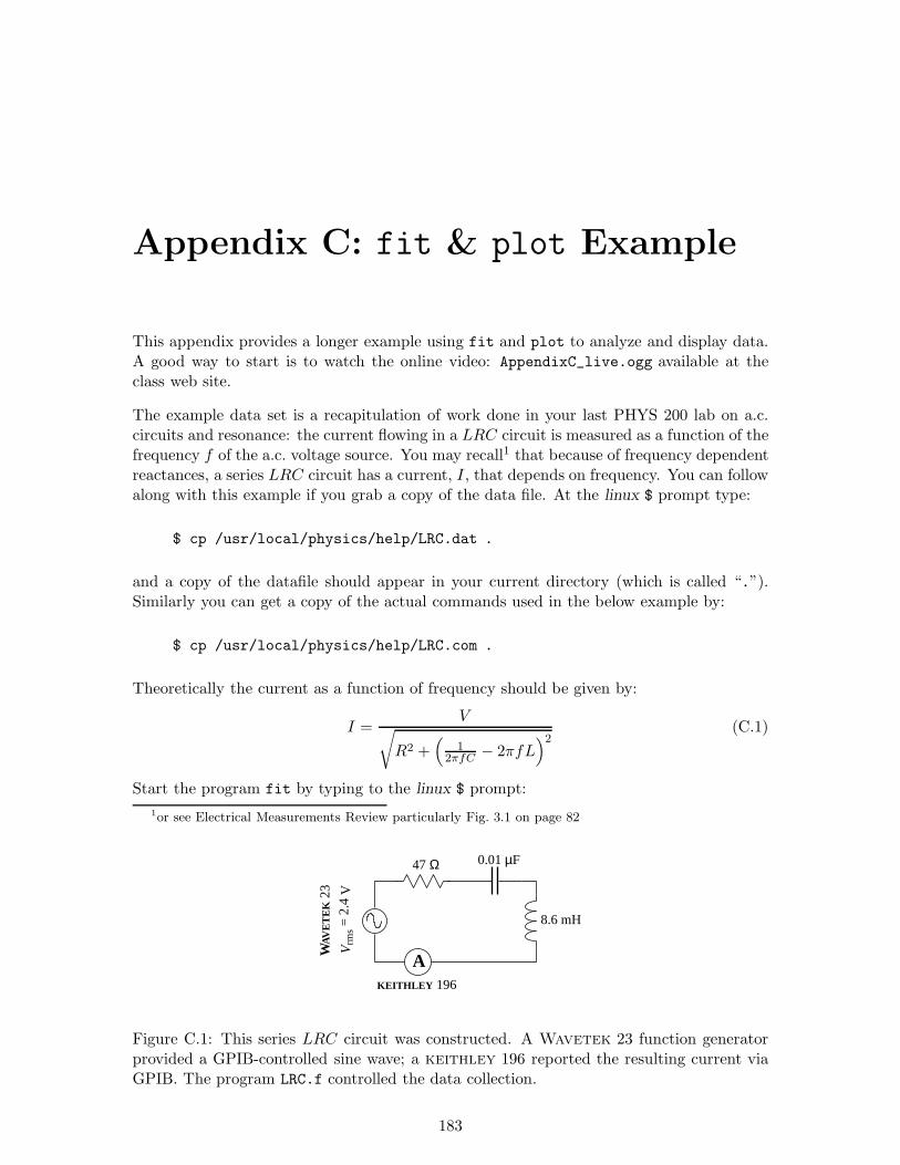
Appendix C: fit & plot Example

This appendix provides a longer example using fit and plot to analyze and display data.A good way to start is to watch the online video: AppendixC_live.ogg available at theclass web site.

The example data set is a recapitulation of work done in your last PHYS 200 lab on a.c.circuits and resonance: the current flowing in a LRC circuit is measured as a function of thefrequency f of the a.c. voltage source. You may recall1 that because of frequency dependentreactances, a series LRC circuit has a current, I, that depends on frequency. You can followalong with this example if you grab a copy of the data file. At the linux $ prompt type:

$ cp /usr/local/physics/help/LRC.dat .

and a copy of the datafile should appear in your current directory (which is called “.”).Similarly you can get a copy of the actual commands used in the below example by:

$ cp /usr/local/physics/help/LRC.com .

Theoretically the current as a function of frequency should be given by:

I =V

√

R2 +(

12πfC − 2πfL

)2(C.1)

Start the program fit by typing to the linux $ prompt:

1or see Electrical Measurements Review particularly Fig. 3.1 on page 82

0.01 µF

Vrm

s = 2

.4 V

A

47 Ω

KEITHLEY 196

WA

VE

TE

K 2

3

8.6 mH

Figure C.1: This series LRC circuit was constructed. A Wavetek 23 function generatorprovided a GPIB-controlled sine wave; a keithley 196 reported the resulting current viaGPIB. The program LRC.f controlled the data collection.

183

184 Appendix C: fit & plot Example

$ fit

*

The program responds with its own prompt: * . We need to tell fit the name of the datafilewe want to analyze and then read in that data:

* set file=LRC.dat

* read

freq(Hz) I(A) dI(A) by default this line ignored!

READ Done.

The first line of the file (freq(Hz). . . ) is simply echoed back as a way of confirming thatyou are reading the intended file. It should be noted the file LRC.dat was written in thedefault form, with x values in the first column (XCOL=1) , y values in the second column(YCOL=2), and y-error values in the third column (YECOL=3). Next we need to tell fit whatfunction should match the data.

* set f(x)=k1/sqrt(k2^2+(1/(2*pi*k3*x)-2*pi*k4*x)^2)

where V = k1, R = k2, C = k3, L = k4 and f = x. For nonlinear fits we must always givestarting parameter estimates. In this case that’s easy as I measured the component valueswhen I built the circuit:

* set k1=2.4 k2=47 k3=1e-8 k4=.0086

Next I command a fit: please adjust the parameters k1–k4 to achieve the smallest possiblereduced χ2:

* fit

Enter list of Ks to vary, e.g. K1-K3,K5 k1-k4

FIT finished with change in chi-square= 1.5258789E-04

6 iterations used

REDUCED chi-squared= 3.790897 chi-squared= 363.9261

K1= 2.262721 K2= 190.7750 K3= 0.9930065E-08

K4= 0.8230284E-02

Display covariance/curvature matrices? No, Screen, File [N,S,F]

The result is pretty much as expected: reduced χ2 is high, but in the usually acceptablerange, the parameters are close to my original guess, with the exception of k2 = R. Onreflection even R is OK as the inductor itself has resistance (77.8 Ω) and according toFig. 3.1 on page 82, the function generator also has an internal 50 Ω resistor. Thus:47 + 77.8 + 50 = 167.8 Ω should have been expected. Currently fit is asking if I want tolook at the covariance matrix, but I’ll delay replying No, Screen, or File until I look at thefitted curve.

I start another terminal to display, using the program plot, what the fitted curve lookslike: at the linux $ prompt I type:

Appendix C: fit & plot Example 185

$ plot

A new blue terminal (labeled plot.exe) pops up with its own * prompt. Exactly as withfit I must tell the program the name of the datafile and then read in the data:

* set file LRC.dat

* read

freq(Hz) I(A) dI(A) by default this line ignored!

READ Done.

The x-data (frequency) ranges from 10000 to 30000; y-data (current) ranges from .002 to.012. I could set by hand those ranges (e.g., XMIN=10000), but its much easier to have theprogram make what it thinks are reasonable choices using the command:

* scale

I could now draw a border and display the datapoints, but first I tell plot the proper axeslabels:

* set xlabel=’Frequency (Hz)’ ylabel="RMS Current (A)" title=Resonance

* border

* dpoint

Plot is to use exactly the same function as fit:

* set f(x)=k1/sqrt(k2^2+(1/(2*pi*k3*x)-2*pi*k4*x)^2)

and I can copy&paste2 from the fit screen the values fit found for those parameters:

* set K1= 2.262721 K2= 190.7750 K3= 0.9930065E-08

* set K4= 0.8230284E-02

Then I can have plot display that function curve and print a hardcopy:

* fcurve

* pcopy

2Warning repeated: Ctrl C kills not copies; highlight and middle-mouse for copy

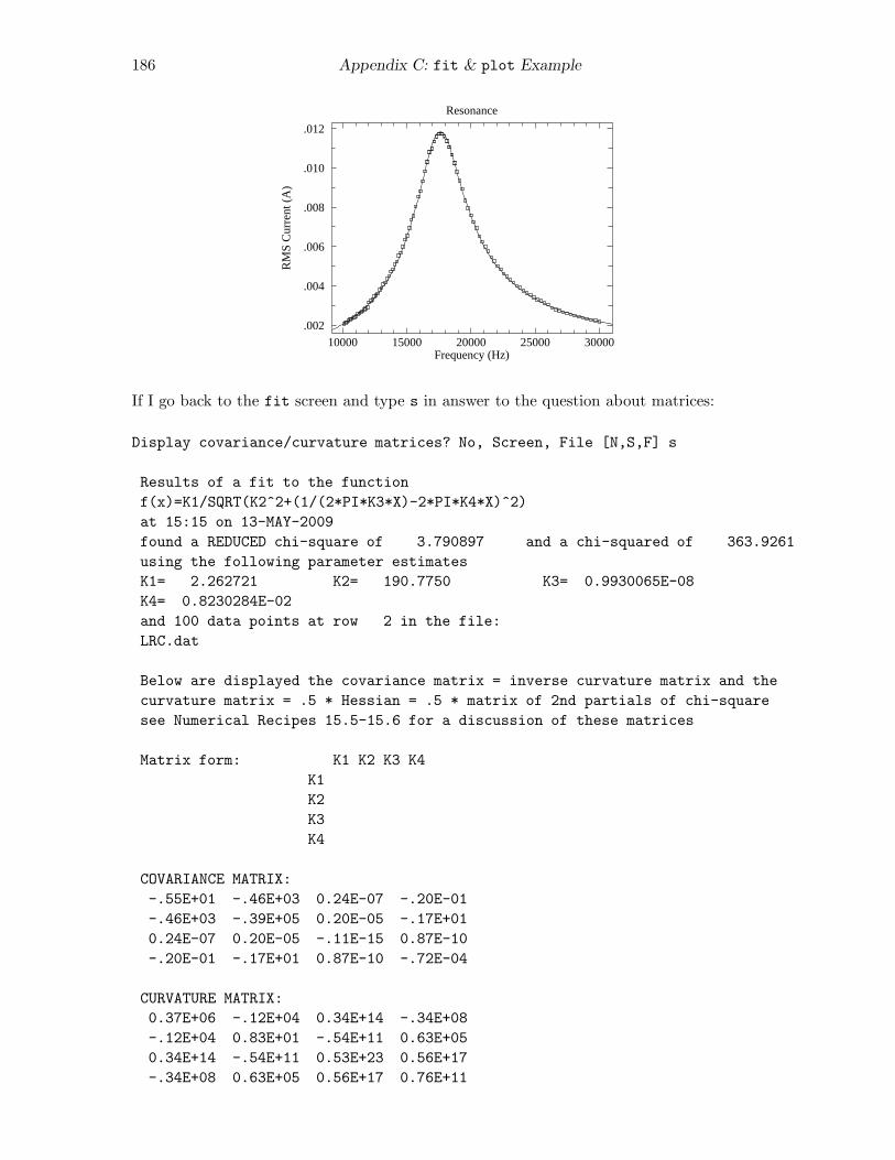
186 Appendix C: fit & plot Example

10000 15000 20000 25000 30000

.012

.010

.008

.006

.004

.002

Resonance

Frequency (Hz)

RM

S C

urre

nt (

A)

If I go back to the fit screen and type s in answer to the question about matrices:

Display covariance/curvature matrices? No, Screen, File [N,S,F] s

Results of a fit to the function

f(x)=K1/SQRT(K2^2+(1/(2*PI*K3*X)-2*PI*K4*X)^2)

at 15:15 on 13-MAY-2009

found a REDUCED chi-square of 3.790897 and a chi-squared of 363.9261

using the following parameter estimates

K1= 2.262721 K2= 190.7750 K3= 0.9930065E-08

K4= 0.8230284E-02

and 100 data points at row 2 in the file:

LRC.dat

Below are displayed the covariance matrix = inverse curvature matrix and the

curvature matrix = .5 * Hessian = .5 * matrix of 2nd partials of chi-square

see Numerical Recipes 15.5-15.6 for a discussion of these matrices

Matrix form: K1 K2 K3 K4

K1

K2

K3

K4

COVARIANCE MATRIX:

-.55E+01 -.46E+03 0.24E-07 -.20E-01

-.46E+03 -.39E+05 0.20E-05 -.17E+01

0.24E-07 0.20E-05 -.11E-15 0.87E-10

-.20E-01 -.17E+01 0.87E-10 -.72E-04

CURVATURE MATRIX:

0.37E+06 -.12E+04 0.34E+14 -.34E+08

-.12E+04 0.83E+01 -.54E+11 0.63E+05

0.34E+14 -.54E+11 0.53E+23 0.56E+17

-.34E+08 0.63E+05 0.56E+17 0.76E+11

Appendix C: fit & plot Example 187

The error results are a total disaster! The usual rule is that the error in a parameter is givenby the square root of the diagonal element of the covariance matrix. Thus (supposedly):

δk1 =√

−.55× 101 (C.2)

δk2 =√

−.39× 105 (C.3)

δk3 =√

−.11× 10−15 (C.4)

δk4 =√

−.72× 10−4 (C.5)

Clearly this is some sort of nonsense as the errors cannot be imaginary. Further note thatin every case |δki| ∼ ki.

A hint about what’s going on is gained by making a different starting guess for the valuesof the parameters:

* set k1=240 k2=.47 k3=1e-7 k4=.00086

Fit results show the same reduced χ2, but with radically different parameters:

REDUCED chi-squared= 3.790896 chi-squared= 363.9260

K1= 0.2419768 K2= 20.40159 K3= 0.9285606E-07

K4= 0.8801518E-03

There is a curve of (L,R,C, V ) values that produces exactly the same resonance curve.Substituting

L → αL (C.6)

C → C/α (C.7)

R → αR (C.8)

V → αV (C.9)

(C.10)

into Eq. C.1 results in an unchanged function (the α cancels out).

We can rewrite our function with just three parameters:

I =I0

√

1 +Q2(

f0f − f

f0

)2(C.11)

where:

I0 = V/R (C.12)

Q =

√

L/C

R(C.13)

f0 =1

2π√LC

(C.14)

(C.15)

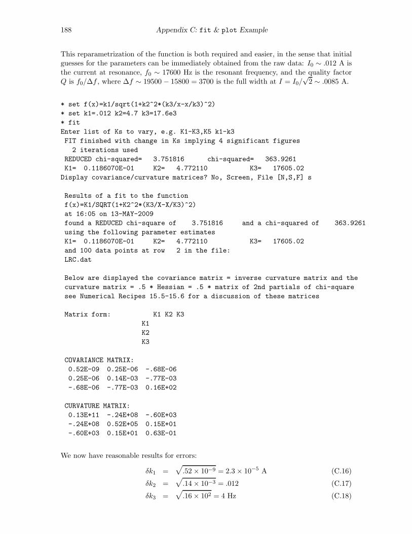
188 Appendix C: fit & plot Example

This reparametrization of the function is both required and easier, in the sense that initialguesses for the parameters can be immediately obtained from the raw data: I0 ∼ .012 A isthe current at resonance, f0 ∼ 17600 Hz is the resonant frequency, and the quality factorQ is f0/∆f , where ∆f ∼ 19500 − 15800 = 3700 is the full width at I = I0/

√2 ∼ .0085 A.

* set f(x)=k1/sqrt(1+k2^2*(k3/x-x/k3)^2)

* set k1=.012 k2=4.7 k3=17.6e3

* fit

Enter list of Ks to vary, e.g. K1-K3,K5 k1-k3

FIT finished with change in Ks implying 4 significant figures

2 iterations used

REDUCED chi-squared= 3.751816 chi-squared= 363.9261

K1= 0.1186070E-01 K2= 4.772110 K3= 17605.02

Display covariance/curvature matrices? No, Screen, File [N,S,F] s

Results of a fit to the function

f(x)=K1/SQRT(1+K2^2*(K3/X-X/K3)^2)

at 16:05 on 13-MAY-2009

found a REDUCED chi-square of 3.751816 and a chi-squared of 363.9261

using the following parameter estimates

K1= 0.1186070E-01 K2= 4.772110 K3= 17605.02

and 100 data points at row 2 in the file:

LRC.dat

Below are displayed the covariance matrix = inverse curvature matrix and the

curvature matrix = .5 * Hessian = .5 * matrix of 2nd partials of chi-square

see Numerical Recipes 15.5-15.6 for a discussion of these matrices

Matrix form: K1 K2 K3

K1

K2

K3

COVARIANCE MATRIX:

0.52E-09 0.25E-06 -.68E-06

0.25E-06 0.14E-03 -.77E-03

-.68E-06 -.77E-03 0.16E+02

CURVATURE MATRIX:

0.13E+11 -.24E+08 -.60E+03

-.24E+08 0.52E+05 0.15E+01

-.60E+03 0.15E+01 0.63E-01

We now have reasonable results for errors:

δk1 =√

.52× 10−9 = 2.3 × 10−5 A (C.16)

δk2 =√

.14× 10−3 = .012 (C.17)

δk3 =√

.16× 102 = 4 Hz (C.18)

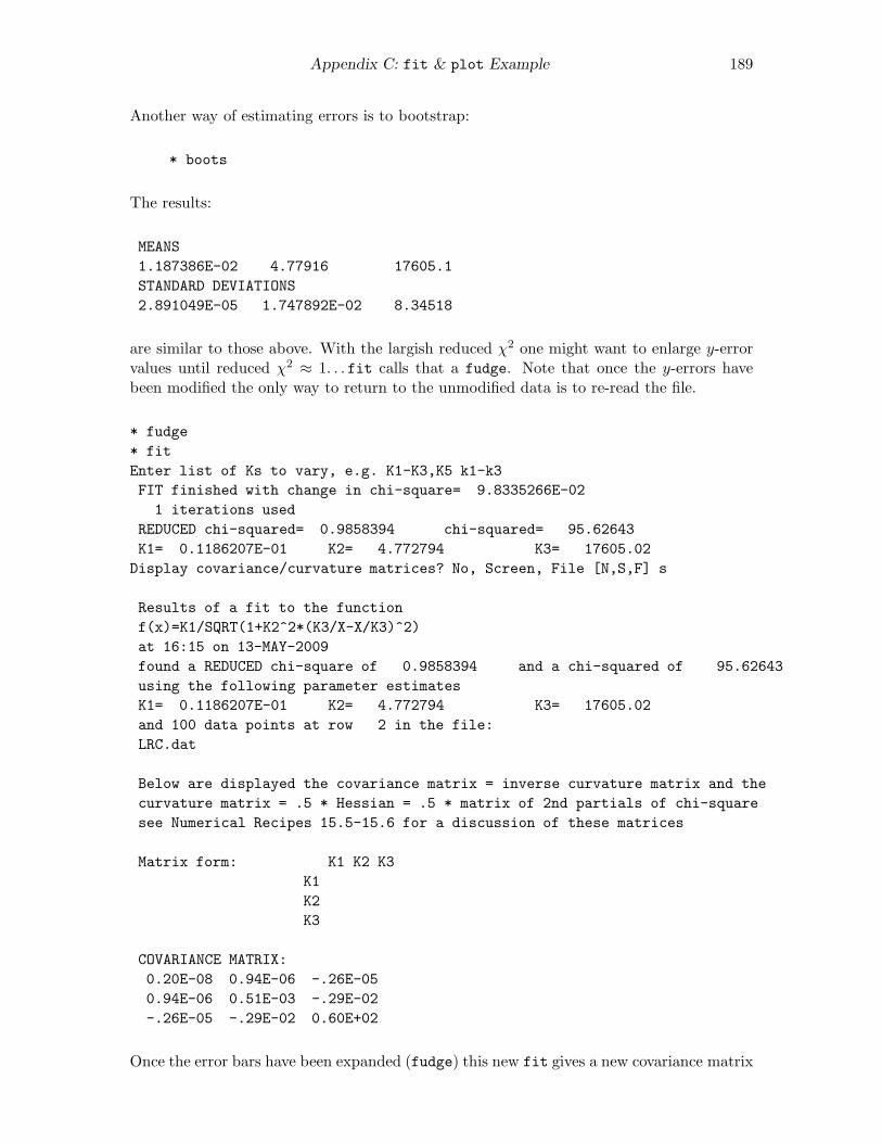
Appendix C: fit & plot Example 189

Another way of estimating errors is to bootstrap:

* boots

The results:

MEANS

1.187386E-02 4.77916 17605.1

STANDARD DEVIATIONS

2.891049E-05 1.747892E-02 8.34518

are similar to those above. With the largish reduced χ2 one might want to enlarge y-errorvalues until reduced χ2 ≈ 1. . . fit calls that a fudge. Note that once the y-errors havebeen modified the only way to return to the unmodified data is to re-read the file.

* fudge

* fit

Enter list of Ks to vary, e.g. K1-K3,K5 k1-k3

FIT finished with change in chi-square= 9.8335266E-02

1 iterations used

REDUCED chi-squared= 0.9858394 chi-squared= 95.62643

K1= 0.1186207E-01 K2= 4.772794 K3= 17605.02

Display covariance/curvature matrices? No, Screen, File [N,S,F] s

Results of a fit to the function

f(x)=K1/SQRT(1+K2^2*(K3/X-X/K3)^2)

at 16:15 on 13-MAY-2009

found a REDUCED chi-square of 0.9858394 and a chi-squared of 95.62643

using the following parameter estimates

K1= 0.1186207E-01 K2= 4.772794 K3= 17605.02

and 100 data points at row 2 in the file:

LRC.dat

Below are displayed the covariance matrix = inverse curvature matrix and the

curvature matrix = .5 * Hessian = .5 * matrix of 2nd partials of chi-square

see Numerical Recipes 15.5-15.6 for a discussion of these matrices

Matrix form: K1 K2 K3

K1

K2

K3

COVARIANCE MATRIX:

0.20E-08 0.94E-06 -.26E-05

0.94E-06 0.51E-03 -.29E-02

-.26E-05 -.29E-02 0.60E+02

Once the error bars have been expanded (fudge) this new fit gives a new covariance matrix

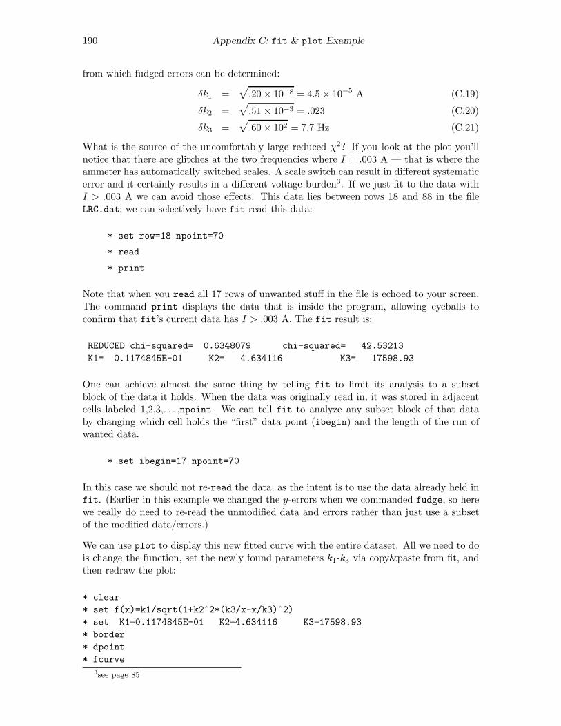
190 Appendix C: fit & plot Example

from which fudged errors can be determined:

δk1 =√

.20× 10−8 = 4.5 × 10−5 A (C.19)

δk2 =√

.51× 10−3 = .023 (C.20)

δk3 =√

.60× 102 = 7.7 Hz (C.21)

What is the source of the uncomfortably large reduced χ2? If you look at the plot you’llnotice that there are glitches at the two frequencies where I = .003 A — that is where theammeter has automatically switched scales. A scale switch can result in different systematicerror and it certainly results in a different voltage burden3. If we just fit to the data withI > .003 A we can avoid those effects. This data lies between rows 18 and 88 in the fileLRC.dat; we can selectively have fit read this data:

* set row=18 npoint=70

* read

* print

Note that when you read all 17 rows of unwanted stuff in the file is echoed to your screen.The command print displays the data that is inside the program, allowing eyeballs toconfirm that fit’s current data has I > .003 A. The fit result is:

REDUCED chi-squared= 0.6348079 chi-squared= 42.53213

K1= 0.1174845E-01 K2= 4.634116 K3= 17598.93

One can achieve almost the same thing by telling fit to limit its analysis to a subsetblock of the data it holds. When the data was originally read in, it was stored in adjacentcells labeled 1,2,3,. . . ,npoint. We can tell fit to analyze any subset block of that databy changing which cell holds the “first” data point (ibegin) and the length of the run ofwanted data.

* set ibegin=17 npoint=70

In this case we should not re-read the data, as the intent is to use the data already held infit. (Earlier in this example we changed the y-errors when we commanded fudge, so herewe really do need to re-read the unmodified data and errors rather than just use a subsetof the modified data/errors.)

We can use plot to display this new fitted curve with the entire dataset. All we need to dois change the function, set the newly found parameters k1-k3 via copy&paste from fit, andthen redraw the plot:

* clear

* set f(x)=k1/sqrt(1+k2^2*(k3/x-x/k3)^2)

* set K1=0.1174845E-01 K2=4.634116 K3=17598.93

* border

* dpoint

* fcurve

3see page 85

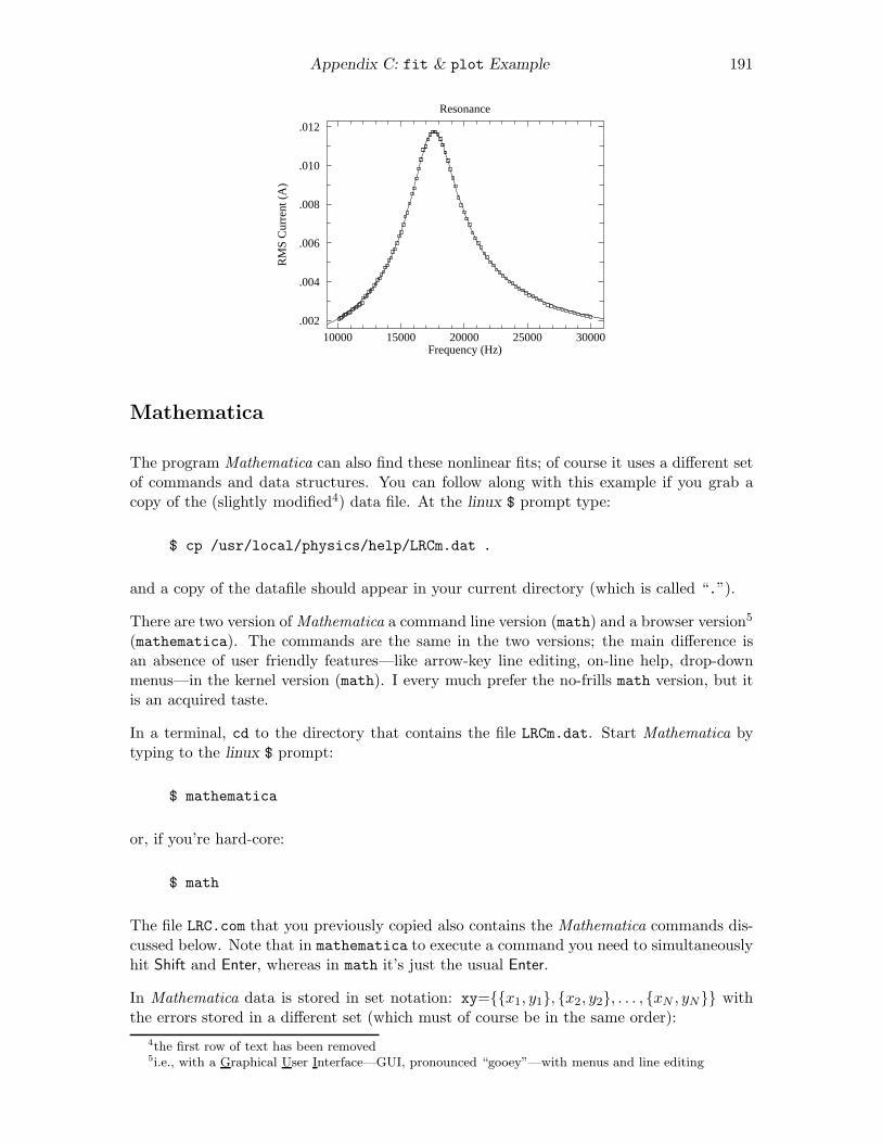
Appendix C: fit & plot Example 191

10000 15000 20000 25000 30000

.012

.010

.008

.006

.004

.002

Resonance

Frequency (Hz)

RM

S C

urre

nt (

A)

Mathematica

The program Mathematica can also find these nonlinear fits; of course it uses a different setof commands and data structures. You can follow along with this example if you grab acopy of the (slightly modified4) data file. At the linux $ prompt type:

$ cp /usr/local/physics/help/LRCm.dat .

and a copy of the datafile should appear in your current directory (which is called “.”).

There are two version of Mathematica a command line version (math) and a browser version5

(mathematica). The commands are the same in the two versions; the main difference isan absence of user friendly features—like arrow-key line editing, on-line help, drop-downmenus—in the kernel version (math). I every much prefer the no-frills math version, but itis an acquired taste.

In a terminal, cd to the directory that contains the file LRCm.dat. Start Mathematica bytyping to the linux $ prompt:

$ mathematica

or, if you’re hard-core:

$ math

The file LRC.com that you previously copied also contains the Mathematica commands dis-cussed below. Note that in mathematica to execute a command you need to simultaneouslyhit Shift and Enter, whereas in math it’s just the usual Enter.

In Mathematica data is stored in set notation: xy=x1, y1, x2, y2, . . . , xN , yN withthe errors stored in a different set (which must of course be in the same order):

4the first row of text has been removed5i.e., with a Graphical User Interface—GUI, pronounced “gooey”—with menus and line editing

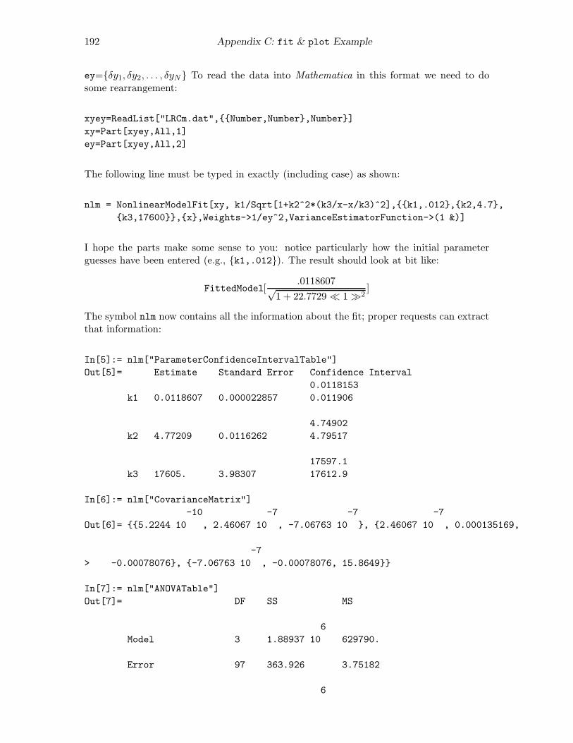
192 Appendix C: fit & plot Example

ey=δy1, δy2, . . . , δyN To read the data into Mathematica in this format we need to dosome rearrangement:

xyey=ReadList["LRCm.dat",Number,Number,Number]

xy=Part[xyey,All,1]

ey=Part[xyey,All,2]

The following line must be typed in exactly (including case) as shown:

nlm = NonlinearModelFit[xy, k1/Sqrt[1+k2^2*(k3/x-x/k3)^2],k1,.012,k2,4.7,

k3,17600,x,Weights->1/ey^2,VarianceEstimatorFunction->(1 &)]

I hope the parts make some sense to you: notice particularly how the initial parameterguesses have been entered (e.g., k1,.012). The result should look at bit like:

FittedModel[.0118607√

1 + 22.7729 ≪ 1 ≫2]

The symbol nlm now contains all the information about the fit; proper requests can extractthat information:

In[5]:= nlm["ParameterConfidenceIntervalTable"]

Out[5]= Estimate Standard Error Confidence Interval

0.0118153

k1 0.0118607 0.000022857 0.011906

4.74902

k2 4.77209 0.0116262 4.79517

17597.1

k3 17605. 3.98307 17612.9

In[6]:= nlm["CovarianceMatrix"]

-10 -7 -7 -7

Out[6]= 5.2244 10 , 2.46067 10 , -7.06763 10 , 2.46067 10 , 0.000135169,

-7

> -0.00078076, -7.06763 10 , -0.00078076, 15.8649

In[7]:= nlm["ANOVATable"]

Out[7]= DF SS MS

6

Model 3 1.88937 10 629790.

Error 97 363.926 3.75182

6

Appendix C: fit & plot Example 193

Uncorrected Total 100 1.88974 10

Corrected Total 99 377421.

ParameterConfidenceIntervalTable gives us the fitted parameters with usual errors. Aswith fit, these estimates are the square root of the diagonal elements of the CovarianceMatrix.The quality of the fit is available in the ANOVATable: the Error row, the SS column is theχ2 and the MS column is the reduced χ2.

Mathematica needs some help to do plots with error bars. Additionally the error bars andthe data need to be put together in exactly the right way:

Needs["ErrorBarPlots‘"]

bar=Map[ErrorBar,ey]

xyEB=Transpose[xy,bar]

ErrorListPlot[xyEB]

Show[ErrorListPlot[xyEB], Plot[nlm[x], x, 10000, 30000], Frame->True]

194 Appendix C: fit & plot Example

Appendix D: Linux Commands

195

196 Appendix D: Linux Commands

Appendix E: Error Formulae

197

198 Appendix E: Error Formulae

Uncertainty Formulae

In the below equations the quantities a, b, c, . . . have uncertainties δa, δb, δc, . . . whereasthe quantities K, k1, k2, . . . are “constants” (like π or 2) with zero error or quantitieswith so small error that they can be treated as error-free (like the mass of a proton:mp = (1.67262158 ± .00000013) × 10−27 kg or Avogadro’s number NA = (6.02214199 ±.0000047)×1023). This table reports the error in a calculated quantity R (which is assumedto be positive). Note that a quantity like δa is called an absolute error; whereas the quantityδa/a is called the relative error (or, when multiplied by 100, the percent error). The oddPythagorean-theorem-like addition (e.g., δR =

√δa2 + δb2) is called “addition in quadra-

ture”. Thus the formula for the error in R = K ab/cd could be stated as “the percent errorin R is the sum of the percent errors in a, b, c and d added in quadrature”.

Equation Uncertainty

R = a+K δR = δa (E.1)

R = K aδR

R=δa

aor δR = |K| δa (E.2)

R =K

a

δR

R=δa

aor δR =

|K| δaa2

(E.3)

R = K ak1δR

R=

|k1| δaa

or δR = |k1Kak1−1| δa (E.4)

R = a± b δR =√

δa2 + δb2 (E.5)

R = k1a+ k2b δR =

√

(k1δa)2 + (k2δb)

2 (E.6)

R = K abδR

R=

√

(

δa

a

)2

+

(

δb

b

)2

(E.7)

R = Ka

b

δR

R=

√

(

δa

a

)2

+

(

δb

b

)2

(E.8)

R = f(a) δR = |f ′(a)| δa (E.9)

R = Kab

cd

δR

R=

√

(

δa

a

)2

+

(

δb

b

)2

+

(

δc

c

)2

+

(

δd

d

)2

(E.10)

R = Kak1bk2

ck3dk4δR

R=

√

(

k1δa

a

)2

+

(

k2δb

b

)2

+

(

k3δc

c

)2

+

(

k4δd

d

)2

(E.11)

R = f(a, b, c, d) δR =

√

(

∂f

∂aδa

)2

+

(

∂f

∂bδb

)2

+

(

∂f

∂cδc

)2

+

(

∂f

∂dδd

)2

(E.12)

Appendix E: Error Formulae 199