physics 200 laboratory manual - tools for science
TRANSCRIPT

PHYSICS 200LABORATORY MANUAL
FOUNDATIONS OF PHYSICS II
Spring 2010

2

Contents
Introduction . . . . . . . . . . . . . . . . . . . . . . . . . . . . . . . . . . . . . . . 5
1. Field Superposition . . . . . . . . . . . . . . . . . . . . . . . . . . . . . . . . . 11
2. Equipotentials and Electric Field Lines . . . . . . . . . . . . . . . . . . . . . . 17
3. The Digital Oscilloscope . . . . . . . . . . . . . . . . . . . . . . . . . . . . . . 25
4. Electrical Circuits . . . . . . . . . . . . . . . . . . . . . . . . . . . . . . . . . . 37
5. RC Circuits . . . . . . . . . . . . . . . . . . . . . . . . . . . . . . . . . . . . . 49
6. Ohmic & Non-Ohmic Circuit Elements . . . . . . . . . . . . . . . . . . . . . . 57
7. e/m of the Electron . . . . . . . . . . . . . . . . . . . . . . . . . . . . . . . . . 63
8. Helmholtz Coils . . . . . . . . . . . . . . . . . . . . . . . . . . . . . . . . . . . 69
9. AC Circuits . . . . . . . . . . . . . . . . . . . . . . . . . . . . . . . . . . . . . 75
Appendix A — Least Squares Fits . . . . . . . . . . . . . . . . . . . . . . . . . . 85
Appendix B — Meter Uncertainty Specifications . . . . . . . . . . . . . . . . . . 93
Appendix C — Uncertainty Formulae . . . . . . . . . . . . . . . . . . . . . . . . 97
3

4

Introduction
Purpose
By a careful and diligent study of natural laws I trust that we shall at leastescape the dangers of vague and desultory modes of thought and acquire a habitof healthy and vigorous thinking which will enable us to recognise error in allthe popular forms in which it appears and to seize and hold fast truth whetherit be old or new. . . [But] I have no reason to believe that the human intellect isable to weave a system of physics out of its own resources without experimentallabour. Whenever the attempt has been made it has resulted in an unnaturaland self-contradictory mass of rubbush. James Clerk Maxwell
Physics and engineering rely on quantitative experiments. Experiments are designed sim-plifications of nature: line drawings rather than color photographs. The hope is that bystripping away the details, the essence of nature is revealed. (Of course, the critics of sciencewould argue that the essence of nature is lost in simplification: a dissected frog is no longer afrog.) While the aim of experiment is appropriate simplification, the design of experimentsis anything but simple. Typically it involves days (weeks, months, . . . ) of “fiddling” beforethe experiment finally “works”. I wish this sort of creative problem-oriented process couldbe taught in a scheduled lab period, but limited time and the many prerequisites make thisimpossible. Look for more creative labs starting next year!
Thus this Lab Manual describes experiences (“labs”) that are a caricature of experimentalphysics. Our labs will typically emphasize thorough preparation, an underlying mathemati-cal model of nature, good experimental technique, analysis of data (including the significanceof error) . . . the basic prerequisites for doing science. But your creativity will be circum-scribed. You will find here “instructions” which are not a part of real experiments (wherethe methods and/or outcomes are not known in advance). In my real life as a physicist, Ihave little use for “instructions”, but I’m going to try and force you to follow them in thiscourse. (This year: follow what I say—not what I do.)
The goals of these labs are therefore limited. You will:
1. Perform experiments that illustrate the foundations of electricity and magnetism.
2. Become acquainted with some commonly used electronic lab equipment (meters,scopes, sources, etc).
3. Perform basic measurements and recognize the associated limitations (which, whenexpressed as a number, are called uncertainties or errors).
5
6 Introduction
4. Practice the methods which allow you to determine how uncertainties in measuredquantities propagate to produce uncertainties in calculated quantities.
5. Practice the process of verifying a mathematical model, including data collection, datadisplay, and data analysis (particularly graphical data analysis with curve fitting).
6. Practice the process of keeping an adequate lab notebook.
7. Experience the process of “fiddling” with an experiment until it finally “works”.
8. Develop an appreciation for the highs and lows of lab work. And I hope: learn tolearn from the lows.
Lab Schedule
The lab schedule can be found in the course syllabus. You should be enrolled in a lab sectionfor PHYS 200 and you should perform and complete the lab that day/time. Problemsmeeting the schedule should be addressed—well in advance—to the lab manager.
Materials
You should bring the following to each lab:
• Lab notebook. You will need three notebooks: While one is being graded, the otherswill be available to use in the following labs. The lab notebook should have quad-ruledpaper (so that it can be used for graphs) and a sewn binding (for example, Ampad#26–251, available in the campus bookstores). The notebooks may be “used” (forexample, those used in PHYS 191).
• Lab Manual (this one)
• The knowledge you gained from carefully reading the Lab Manual before you attended.
• A calculator, preferably scientific.
• A straightedge (for example, a 6” ruler).
• A pen (we prefer your lab book be written in ink, since you’re not supposed to erase).
Before Lab:
Since you have a limited time to use equipment (other students will need it), it will be toyour advantage if you come to the laboratory well prepared. Please read the description ofthe experiment carefully, and do any preliminary work in your lab notebook before you cometo lab. Note carefully (perhaps by underlining) questions included in the lab description.Typically you will lose points if you fail to answer every question.
Introduction 7
During Lab:
Note the condition of your lab station when you start so that you can return it to that statewhen you leave. Check the apparatus assigned to you. Be sure you know the function ofeach piece of equipment and that all the required pieces are present. If you have questions,ask your instructor. Usually you will want to make a sketch of the setup in your notebook.Prepare your experimental setup and decide on a procedure to follow in collecting data.Keep a running outline in your notebook of the procedure actually used. If the procedureused is identical to that in this Manual, you need only note “see Manual”. Nevertheless,an outline of your procedure can be useful even if you aim to exactly follow the Manual.Prepare tables for recording data (leave room for calculated quantities). Write your datain your notebook as you collect it!
Check your data table and graph, and make sample calculations, if pertinent, to see ifeverything looks satisfactory before going on to something else. Most physical quantities willappear to vary continuously and thus yield a smooth curve. If your data looks questionable(e.g., a jagged, discontinuous “curve”) you should take some more data near the points inquestion. Check with the instructor if you have any doubts.
Complete the analysis of data in your notebook and indicate your final results clearly. Ifyou make repeated calculations of any quantity, you need only show one sample calculation.Often a spreadsheet will be used to make repeated calculations. In this case it is particularlyimportant to report how each column was calculated. Tape computer-generated data tables,plots and least-squares fit reports into your notebook so that they can be examined easily.Answer all questions that were asked in the Lab Manual.
CAUTION: for your protection and for the good of the equipment, please check with theinstructor before turning on any electrical devices.
Lab Notebook
Your lab notebook should represent a detailed record of what you have done in the labora-tory. It should be complete enough so that you could look back on this notebook after ayear or two and reconstruct your work.
Your notebook should include your preparation for lab, sketches and diagrams to explainthe experiment, data collected, initial graphs (done as data is collected), comments ondifficulties, sample calculations, data analysis, final graphs, results, and answers to questionsasked in the Lab Manual. NEVER delete, erase, or tear out sections of your notebook thatyou want to change. Instead, indicate in the notebook what you want to change and why(such information can be valuable later on). Then lightly draw a line through the unwantedsection and proceed with the new work.
DO NOT collect data or other information on other sheets of paper and then transfer toyour notebook. Your notebook is to be a running record of what you have done, not aformal (all errors eliminated) report. There will be no formal lab reports in this course.When you have finished a particular lab, you turn in your notebook.
Ordinarily, your notebook should include the following items for each experiment.

8 Introduction
NAMES. The title of the experiment, your name, your lab partner’s name, and your labstation number.
DATES. The date the experiment was performed.
PURPOSE. A brief statement of the objective or purpose of the experiment.
THEORY. At least a listing of the relevant equations, and what the symbols represent.Often it is useful to number these equations so you can unambiguously refer to them.
Note: These first four items can usually be completed before you come to lab.
PROCEDURE. This section should be an outline of what you did in lab. As an absoluteminimum your procedure must clearly describe the data. For example, a column ofnumbers labeled “voltage” is not sufficient. You must identify how the voltage wasmeasured, the scale settings on the voltmeter, etc. Your diagram of the apparatus(see below) is usually a critical part of this description, as it is usually easier to drawhow the data were measured than describe it in words. Sometimes your procedurewill be identical to that described in the Lab Manual, in which case the proceduremay be abbreviated to something like: “following the procedure in the Lab Manual,we used apparatus Z to measure Y as we varied X”. However there are usually detailsyou can fill in about the procedure. Your procedure may have been different fromthat described in the Lab Manual. Or points that seem important to you may nothave been included. And so on. This section is also a good place to describe anydifficulties you encountered in getting the experiment set up and working.
DIAGRAMS. A sketch of the apparatus is almost always required. A simple blockdiagram can often describe the experiment better than a great deal of written expla-nation.
DATA. You should record in your notebook (or perhaps a spreadsheet) a concurrentrecord of your relevant observations (the actual immediately observed data not arecopied version). You should record all the numbers (including every digit displayedby meters) you encounter, including units and uncertainties. If you find it difficult tobe neat and organized while the experiment is in progress, you might try using theleft-hand pages of your notebook for doodles, raw data, rough calculations, etc., andlater transfer the important items to the right-hand pages. This section often includescomputer-generated data tables, graphs and fit reports — just tape them into yourlab book (one per page please).
You should examine your numbers as they are observed and recorded. Was there anunusual jump? Are intermediate data points required to check a suspicious change?The best way to do this is to graph your data as you acquire it or immediatelyafterward.
CALCULATIONS. Sample calculations should be included to show how results areobtained from the data, and how the uncertainties in the results are related to theuncertainties in the data (see Appendix C). For example, if you calculate the slope ofa straight line, you should record your calculations in detail, something like:
v2 − v1
t2 − t1=
(4.08 − .27) cm/wink
(15 − 1) wink= 0.27214 cm/wink2 (1)
Introduction 9
The grader must be able to reproduce your calculated results based on what youhave recorded in your notebook. The graders are told to totally disregard answersthat appear without an obvious source. It is particularly important to show how eachcolumn in a spreadsheet hardcopy was calculated (quick & easy via ‘self documenting’equations).
RESULTS/CONCLUSIONS. You should end each experiment with a conclusion thatsummarizes your results — what were your results, how successful was the experiment,and what did you learn from it.
This section should begin with a carefully constructed table that collects all of yourimportant numerical results in one place. Numerical values should always includeunits, an appropriate number of significant digits and the experimental error.
You should also compare your results to the theoretical and/or accepted values. Doesyour experimental range of uncertainty overlap the accepted value? Based on yourresults, what does the experiment tell you?
DISCUSSION/CRITIQUE. As a service to us and future students we would appreciateit if you would also include a short critique of the lab in your notebook. Pleasecomment on such things as the clarity of the Lab Manual, performance of equipment,relevance of experiment, timing of the experiment (compared to lecture) and if thereis anything you particularly liked or disliked about the lab. This is a good place toblow off a little steam. Don’t worry; you won’t be penalized, and we use constructivecriticisms to help improve these experiments.
QUICK REPORT. As you leave lab, each lab group should turn in a 3”×5” quick reportcard. You will be told in lab what information belongs on your card. These cards godirectly to the instructor who will use them to identify problems.
Drop off your lab notebook in your lab instructor’s box. Note: The TA’s cannot accept latelabs. If for some reason you cannot complete a lab on time, please see the lab manager (LynnSchultz) in PEngel 139 or call 363–2835. Late labs will only be accepted under exceptionalcircumstances. If an exception is valid, the lab may still be penalized depending on howresponsibly you handled the situation (e.g., did you call BEFORE the lab started?).
Grading
Each lab in your notebook will be graded separately as follows:
9–10 points: A8–8.9 points: B7–7.9 points: C6–6.9 points: D0–5.9 points: Unsatisfactory

10 Introduction

1. Field Superposition
Purpose
The universe is filled with sources of electric and magnetic fields. In this lab you will testthe principle that the field produced by several sources simultaneously is just the vectorsum of the fields produced by each source individually.
Introduction
From Coulomb’s law we know the electric field produced by an isolated charged particle.In a universe of zillions of electrons and protons this result would be without value if welacked a method of finding the field resulting from multiple sources. Electric fields (andalso magnetic fields) combine in the simplest possible way: by vector addition1.
In this experiment we find it convenient to work with magnetic fields rather than electricfields. We have a readily available source of natural magnetic field from the Earth; we canproduce controlled magnetic fields using electromagnets; and we can easily measure thedirection of the magnetic field using an ordinary compass. While you have not yet coveredmagnetic fields in lecture, all you will need to know about them for this lab is that the sourceof magnetic field is electric current and that the magnetic field produced by a current isproportional to that current. Permanent magnets result from orbiting, spinning electronsin iron; Electromagnets result from the easily measured current flowing through copperwires that make up the windings of the coil. (Similar electric currents flowing through themetallic core of the Earth power the Earth’s magnetic field.) Just as an electric field isproportional to the charge that is its source, so the magnetic field of an electromagnet isproportional to its current.
Apparatus
• 1 power supply
• 1 digital multimeter
1Electricity and magnetism is really just one example, as these two things are, as Einstein showed, reallyjust different aspects of one thing: Fµν . Note that many other force fields (for example that in Einstein’stheory of gravity called general relativity) do not satisfy this simple combination rule.
11
12 1: Field Superposition
B
I
I
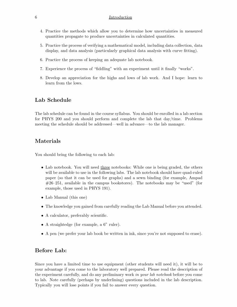
Figure 1.1: Magnetic field lines through a finite solenoid of coils carrying current I.
• 1 solenoid assembly
• 1 compass
• 1 set of leads
Theory
Solenoid
A solenoid is a length of wire wound around a cylinder. Mathematically it is easiest to thinkabout a solenoid as a series of circular loops of wire each carrying the same current, but infact the wire is a tightly spaced helix (spiral). Figure 1.1 shows the magnetic field lines ofa solenoid carrying a current I. The result is perhaps a bit surprising: the magnetic fieldgoes through the core of the cylinder as the current winds around the edge of the cylinder.In a month or so you’ll learn how to calculate the magnetic field for such a solenoid, butfor this lab it is enough to know that the magnetic field is everywhere proportional to thecurrent. In particular, the magnetic field, B, at he center of our solenoid (where we will bedoing our experiment) is given by:
Bs = aI. (1.1)
where I is the electric current flowing around the solenoid (measured in ampere, denoted“A”) and a = 1.14 × 10⁻³ T/A. (The unit of magnetic field is tesla, denoted “T”.) Thesolenoid will be used as an adjustable source of magnetic field.
Earth’s Magnetic Field
The magnetic field of the Earth varies with position and time. However, during the courseof this lab, at your particular lab table, the Earth’s field may be considered constant inmagnitude and direction. (That is the currents producing the Earth’s magnetic field willnot change much during this experiment.) Generally speaking the Earth’s field points north,however here in the northern hemisphere it also points down. The inclination of the field isquite large (over 70) at our latitude.

1: Field Superposition 13
A
Power Supply
Solenoid & Compass Assembly
N
Figure 1.2: Solenoid circuit.
Compass
The needle of a compass points in the direction of the magnetic field it experiences. Wesay that a compass needle shows north, because that is (generally speaking) the directionof the Earth’s magnetic field. The needle is a magnetic dipole made of a small permanentmagnet. Just as an electric dipole feels a torque aligning it to the external electric field, soa magnetic dipole twists until it is aligned with the external magnetic field. We will use thecompass to show us the direction of the magnetic field that results from the superpositionof the Earth’s field with that of the solenoid. While the compass is graduated in degrees,we will find it convenient to work in radians, and so the conversion factor 360 = 2π radianshould be applied to all angles.
Setup
As shown in Figure 1.2, the compass is placed in the center of the solenoid, and the apparatusis oriented so that with no current flowing the compass needle points perpendicular to thecoil-axis in the direction “N”, i.e., θ = 0. When a current is sent through the coil, theneedle will be deflected to point in the direction of the resulting magnetic field. The currentwill be supplied by an adjustable power supply, and accurately measured with a digitalmultimeter. (For more information on the operation of the multimeter see Figure 4.2 onpage 40.) If we denote the magnetic field of the Earth by Be and the magnetic field of thesolenoid by Bs, the resulting total magnetic field should be the vector sum of the two. Asshown in Figure 1.3, we predict
tan θ =Bs
Be=
a
BeI (1.2)
Thus a graph of tan θ vs. I should be a straight line.
Note: since the compass needle is only free to rotate in the horizontal plane, only thehorizontal components of the magnetic field are detected. Thus Be above is actually justthe horizontal component of the Earth’s magnetic field. (Of course, the solenoid has beenoriented so that its field is fully horizontal.) At our latitude it turns out that the verticalcomponent of the Earth’s field is more than twice as large as the horizontal component.

14 1: Field Superposition
Be
Bs
com
bine
d B
θ
Figure 1.3: Adding two magnetic fields: Be from the Earth and Bs from the solenoid. Theangle of the resulting magnetic field is called θ.
Procedure
Position the solenoid/compass assembly such that the compass needle is aligned with north(N) on the compass housing. Without moving the assembly, connect the power supply inseries with the assembly and multimeter as shown in Fig. 1.2. Set the multimeter functionto measure DC amps, denoted: A, on the 20 mA range. After your instructor checksthe circuit, take a series of readings from the compass and multimeter while increasing thecurrent from power supply.
Record about ten well-spaced readings. (Readings should be spaced by about 2 mA or 5,but it is a waste of time to try to make I or θ a round number. Don’t include the θ = 0,I = 0 starting condition as a measurement.)
Reverse the leads on the power supply and take a similar set of measurements. For this lastset of measurements the current, the angle, and the tangent of the angle will be negative.When the measurements have been completed, turn off the power supply and check to seeif the compass is still aligned to the north. If the solenoid/compass assembly has moved,the measurements should be redone.
Calculations will be easier if you put your measured values into a spreadsheet. The uncer-tainty in the current (δI) can be accurately determined from Table 4.1 on page 45, howeverfor this lab an error of 0.5% should be accurate enough. The uncertainty in the compassreading (δθ) must be estimated based on your ability to read the compass scale. Typically,for an analog scale, the uncertainty is estimated to be ± half of the smallest scale division.You may wish to assign a larger uncertainty if you believe the compass is unusually difficultto read. Because computers generally assume angles are in radians, you will need to convertboth θ and δθ to radians!
Lab Report
1. From your uncertainty in θ, determine an uncertainty for each value of y = tan θ.According to calculus, this is:
δ(tan θ) = δθ/(cos θ)2 = δθ(
1 + tan2 θ)
= δθ(1 + y2) (1.3)
1: Field Superposition 15
(This formula can be entered into WAPP+ directly.) Alternatively you can estimateerrors from the difference | tan(θ + δθ) − tan θ| ≈ δ(tan θ). Print your spreadsheetand include it in your notebook. (Remember to self-document your spreadsheet orshow sample calculations.) Make sure you’ve clearly displayed how each column wascalculated.
2. Use WAPP+ (Goggle “wapp+” to find it) to determine the line best approximatingyour tan θ versus I data. (Enter the current and its uncertainty in amperes, not mA.)Tape the fit report and plot in your notebook.
3. Using the best-fit slope, calculate the Earth’s magnetic field, Be, at SJU. (Actuallythis is just the horizontal component of of the Earth’s magnetic field.) A “ballpark”value for Be is 1.5 × 10⁻⁵ T, but magnetic materials in the building will affect theresult. Using the uncertainty in slope, calculate the resulting uncertainty in Be.
4. Complete your lab report with a conclusion and lab critique.

16 1: Field Superposition

2. Equipotentials and Electric FieldLines
A new concept appeared in physics, the most important invention since Newton’stime: the field. It needed great scientific imagination to realize that it is not thecharges nor the particles but the field in the space between the charges and theparticles that is essential for the description of physical phenomena. The fieldconcept proved successful when it led to the formulation of Maxwell’s equationsdescribing the structure of the electromagnetic field.
Einstein & Infield The Evolution Of Physics 1938
Purpose
To explore the concepts of electrostatic potential and electric field and to investigate therelationships between these quantities. To understand how equipotential curves are definedand how they can display the behavior of both the potential and field.
Introduction
Every electric charge in the universe exerts a force on every other electric charge in theuniverse. Alternatively we can introduce the intermediate concept of an electric field. Wethen say that the universe’s charge distribution sets up an electric field ~E at every point inspace, and then that field produces the electric force on any charged particle that happensto be present. The electric field ~E is defined in terms of things we can measure if we bringa “test charge” q to the spot where we want to measure ~E. The electric field is then definedin terms of the total force, ~F, experienced by that test charge q:
~E = ~F/q (2.1)
Note that the field exists independently of any charges that might be used to measure it.For example, fields may be present in a vacuum. At this point is is not obvious1 that the
1Star Wars Episode IV :LUKE: You don’t believe in the Force, do you?HAN: Kid, I’ve flown from one side of this galaxy to the other. I’ve seen a lot of strange stuff, but I’ve
17

18 2: Equipotentials and Electric Field Lines
field concept really explains anything. The utility of the electric field concept lies in thefact that the electric field exists a bit independently of the charges that produce it. Forexample, there is a time delay between changes in the source charge distribution and theforce on distant particles due to propagation delay as the field readjusts to changes in itssource.
The electric force ~F does work (~F · ∆~r) on a charge, q, as it is moved from one point toanother, say from A to B. This work results in a change in the electrical potential energy∆U = UB − UA of the charge. In going from a high potential energy to a low potentialenergy, the force does positive work: WAB = −∆U . Consider, for a moment, a line or surfacealong which the potential energy is constant. No work is done moving along such a line orsurface, and therefore the force cannot have a component in this direction: Electric forces(and hence the electric fields) must be perpendicular to surfaces of constant potentialenergy. This concept is central to our experiment.
Example: Gravitational potential energy. Consider a level surface parallel to thesurface of the Earth. The potential energy mgh does not change along such a surface. Andof course, both the gravitational force m~g, and the gravitational field ~g are perpendicularto this surface, just as we would expect from the above reasoning. Electrical fields andpotential energies are less intuitive because less familiar, but they work in much the sameway.
We can define a new quantity, the potential difference ∆V = VB − VA between points Aand B, in the following way:
∆V =∆U
q= −WAB
q(2.2)
where WAB is the work done by the electric force as the test charge q is moved from A to B.Although the potential energy difference ∆U = UB −UA does depend on q, the ratio ∆U/q(and therefore ∆V ) is independent of q. That is, in a manner analogous to the electric field,potential difference does not depend on the charge q used in its definition, but only on thecharge distribution producing it. Also, since ~F is a conservative force, WAB (and hence thepotential difference) does not depend on the path taken by q in moving from A to B.
Finally, note that only the potential difference has been defined. Specifying the potentialitself at any point depends on assigning a value to the potential at some convenient (andarbitrary) reference point. Often we choose the potential to be zero “at infinity”, i.e., faraway from the source charges, but this choice is arbitrary. Moreover, if we measure onlypotential differences, the choice of “ground” (zero volts) doesn’t matter.
Apparatus
• DC power supply
never seen anything to make me believe there’s one all-powerful force controlling everything. There’s nomystical energy field that controls my destiny.
Of course, we should replace “force” in the above with “field”.

2: Equipotentials and Electric Field Lines 19
DC Source
DMM +
–– +
Probe
Figure 2.1: Electric field mapping circuit.
• digital multimeter (DMM)
• conductive paper with electrode configurations (2)
• card board
• graph paper
• push pins
You will be provided two electrode configurations drawn with a special type of conductingink (graphite suspension) on a special carbon impregnated paper, as sketched in Fig. 2.1.The paper has a very high, but finite, resistance, which allows small currents to flow.Nevertheless, since there is a big difference between the resistance of the conducting inkand the paper, the potential drop within the ink-drawn electrodes is negligible (less than1%) of that across the paper. The potential differences closely resemble those under strictlyelectrostatic (no current) conditions.
Theory
In this experiment you will use different configurations and orientations of electrodes whichhave been painted on very high resistance paper with conducting ink. When the electrodesare connected to a “battery” (actually a DC power supply: a battery eliminator) an electricfield is set up that approximates the electrostatic conditions discussed in lecture. Undertruly electrostatic conditions the charges would be fixed, and the battery could be discon-nected and the electric field would continue undiminished. However, in this experiment thebattery must continue to make up for the charge that leaks between the electrodes throughthe paper. These currents are required for the digital multimeter (DMM) to measure thepotential difference. Nevertheless, the situation closely approximates electrostatic condi-tions and measurement of the potential differences will be similar to those obtained understrictly electrostatic conditions.

20 2: Equipotentials and Electric Field Lines
A 2 A 1
A 4
A 5
B 1 B 2
B 4
B 3
B 5
C 1
C 2
C 3
C 4
C 5
A 3
Figure 2.2: Some equipotential curves for the circle-line electrodes.
Consider Fig. 2.2 where the electrodes are a circle and a line. Suppose we fix one electrodeof the digital multimeter (DMM) at some (arbitrarily chosen) point O and then, using thesecond electrode as a probe, find that set of points A1, A2, A3, . . . such that the potentialdifferences between any of these points and O are equal:
VA1O = VA2O = VA3O = . . . . (2.3)
Hence the potentials at points A1, A2, A3, . . . are equal. In fact, we can imagine a continuumof points tracing out a continuous curve, such that the potential at all the points on thiscurve is the same. Such a curve is called an equipotential. We label this equipotentialVA. We could proceed to find a second set of points, B1, B2, B3, . . . such that the potentialdifference VBnO is the same for n = 1, 2, 3, . . .; i.e.,
VB1O = VB2O = VB3O = . . . . (2.4)
This second set of points defines a second equipotential curve, which we label VB . Theactual values of the potentials assigned to these curves, VA and VB , depend on our choiceof the reference potential VO. However, the potential difference between any two points onthese two equipotentials does not depend on our choice of VO; that is,
(VA − VO) − (VB − VO) = VA − VB (2.5)
and so the potential difference VA − VB can be determined from the measured values VAO
and VBO. A mapping of electrostatic equipotentials is analogous to a contour map oftopographic elevations, since lines of equal elevation are gravitational equipotentials. Theelevation contours are closed curves; that is, one could walk in such a way as to remainalways at the same height above sea level and eventually return to the starting point.Likewise, electrostatic equipotentials are closed curves. The electric field at a given pointis related to the spatial rate of change of the potential at that point, i.e., the gradient, inthe potential. Continuing the analogy with the contour map, we find the electric field is

2: Equipotentials and Electric Field Lines 21
∆xQ
P
V
V+∆V
(a) Two equipotential curves and the mini-mum distance, ∆x, between them.
(b) Orthogonal sets of curves — equipotentials and fieldlines.
Figure 2.3: Equipotential curves
analogous to the slope of the landscape, with the direction of the electric field correspondingto the direction of steepest slope at the point in question. Thus, as shown in Figure 2.3(a),with one equipotential at potential V and a second, nearby one, at potential V + ∆V , themagnitude of the electric field at point P is approximated by
E ≈∣
∣
∣
∣
−∆V
∆x
∣
∣
∣
∣
, (2.6)
where ∆x is the minimum distance between the two equipotentials. Using the minimumvalue of ∆x guarantees that the ‘derivative’
∣
∣−∆V∆x
∣
∣ is largest at the point P . (The derivative
in any direction is determined by the gradient of V : dV = ~∇V ·d~r; the electric field is closelyrelated to the gradient: ~E = − ~∇V . ) The direction of the electric field is in the direction of∆x, either from P to Q, or in the opposite direction, from Q to P , depending upon whether∆V is negative or positive. The minus sign in Eq. (2.6) simply means that the electric fieldis in the direction of decreasing potential. One more property of the gradient is importantto note: the gradient is perpendicular to the tangent to the equipotential at point P , asshown in Fig. 2.3(a). Thus, the electric field is perpendicular to the equipotential curves.
We can now envision two entire families of curves, as illustrated in Figure 2.3(b): the first, aset of equipotentials, and the second, a set of curves whose tangent at a point indicates thedirection of the electric field at that point. The members of the latter family, the electricfield lines, are also called “lines of force” because the electric field is in the direction inwhich a positive charge q would move if it were placed at that point. As mentioned earlier,the equipotentials form closed curves (no beginning, no end), while the field lines starton positive charge and end on negative charge. The two families of curves are orthogonal(perpendicular), because at any given point, say P , the tangent to the equipotential throughP is perpendicular to the field line through P . The direction of a field line is in the directionof the electric field.
The arrows on field lines indicate the direction of the electric field.
Conventionally, equipotential are selected with their potentials in a sequence of uniformsteps (i.e., constant ∆V ). The spacing (∆x) between the equipotentials then immediately

22 2: Equipotentials and Electric Field Lines
gives the relative strength of the corresponding electric field at the point: small ∆x corre-sponding to large E.
Conventionally, the spacing of the field lines is also designed to give a qualitative measureof the magnitude (strength) of the electric field; that is, the field is stronger where thefield lines are more concentrated. (In 3 dimensional space we talk about the “density offield lines”, meaning the number of lines per cross sectional area. In our plane figures, thiscorresponds to the separation between the field lines.) Once the equipotentials have beenmapped, the field lines can be found by drawing the orthogonal family of curves.
Procedure
1. A pair of electrodes have been defined by a pattern painted with conducting silver inkon black high resistance paper. Record (copy or trace) the electrode patterns onto apiece of graph paper. Make copies for each lab partner.
2. Place one of the conductive sheets on the cork board. Connect each painted electrodeto the power supply (battery eliminator) using a positive (+, red) or negative (−,black) wire and a pushpin. Do not break the conducting path of the painted electrodewith a pushpin hole—instead the pushpin should be placed directly alongside thepainted electrode. The pushpin will then press and hold the ring terminal of the wireto the painted electrode without scraping off the paint. You can hold the sheet inplace with additional pins at corners. Connect the black (negative, common or “com”)terminal of the DMM to the negative terminal on the power supply. (Figure 4.2 onpage 40 briefly describes the operation of the multimeter.) You will use the (red) probeconnected to the other voltage terminal of the DMM to measure voltage difference.
3. Have your lab instructor check your set-up. The DMM should be set to read DC Volts(function V), with a range of 20 Volts. Set the power supply to about 10 VoltsDC.
4. With the free probe of the DMM, touch the positive electrode and record the potentialdifference VPO between the two points probed by the DMM. Press firmly to make goodelectrical contact; however, do not puncture or otherwise damage the paper (or thepainted electrode). Touch the DMM probe to various points on the positive electrode.(This may not be possible if the electrode itself is very small, i.e., a “point charge”.)Each electrode should be an equipotential; if the potential seems to vary check thatyou have firm connections to the electrode and contact your instructor if you cannotcorrect the problem.
Touch the free probe of the DMM to the negative electrode and record the (nearlyzero) reading VNO. (Again: this electrode should also be an equipotential. If youcannot achieve an equipotential electrode by reseating the ring terminal on the paintedelectrode, contact your instructor.) In both readings, O refers to a fixed location atthe negative terminal of the power supply. VNO and VPO are the potential differencesbetween the negative (N) and positive (P ) electrodes, and the reference O. ComputeVPN , the potential difference between the positive and negative electrodes.
5. In the vicinity of the negative electrode, find a point where the DMM reads 2.0 Voltsas the free probe is touched to the paper. Remember, do not puncture or otherwise

2: Equipotentials and Electric Field Lines 23
damage the paper. Record this point as accurately as you can on the (white) graphpaper.
Now move the free probe of the DMM to another nearby point where the reading isagain 2.0 V and again record this point on your graph paper. Obtain a series of suchpoints, all corresponding to a DMM reading of 2.0 V, by gradually moving the probefrom point to point. Eventually the set of points will close on itself or, perhaps, gooff the edge of the paper.
6. Repeat the previous step for some other DMM readings, say 3.0 V, 4.0 V, 5.0 V, 6.0V, 7.0 V, and 8.0 V. You should obtain at least five sets of equipotential points.
7. Draw the equipotential curves on the graph paper by connecting the points at thegiven potential with a smooth curve. Each such curve is an equipotential and can belabeled by the appropriate DMM reading.
8. Repeat Steps 2 through 7 for the second electrode configuration.
Analysis
Show your equipotentials to the lab instructor. The instructor will assign a point — call itP — where you should find the electric field.
Carry out the following steps:
1. Draw the tangent to the equipotential through P . (P may have been selected so thatis does not lie on an equipotential you have measured. Nevertheless you should beable to estimate the orientation of that unmeasured equipotential by comparison withthe neighboring, measured equipotentials.)
2. Draw the perpendicular to this tangent through P .
3. Find the distance ∆x, by measuring in cm using a ruler, between two adjacent equipo-tentials, which differ by ∆V . Find the magnitude and direction of the electric field~E at point P , i.e. ~EP . Record the magnitude and indicate the direction by a vectorplaced at P on the graph paper. (∆x could also be defined as the shortest distancebetween the adjacent equipotentials measured along a line the goes through the pointP .)
4. Sketch the field lines orthogonal to the equipotentials for this configuration of elec-trodes, and indicate their direction by small arrowheads. (See Figure 2.3(b).)
5. Repeat Step 4 for the second electrode configuration.

24 2: Equipotentials and Electric Field Lines

3. The Digital Oscilloscope
Purpose
To become familiar with two common lab instruments used with time varying electricalsignals (AC). The function generator produces simple AC signals; the oscilloscope is usedto measure AC signals.
Apparatus
• oscilloscope
• multimeter (DMM)
• function generator
• battery
• microphone
• BNC cables (2)
• “T” adapter
• Banana plug cable with BNC adapter
Introduction
Communication requires signals that change in time. Modern (high volume) electrical com-munication requires electrical signals (voltages, currents) that change rapidly. The digitalmultimeters we’ve used to measure voltage and current can not detect quickly changingsignals (for example AM radio signals) and have significant limitations even at moderatefrequencies (e.g., 20 kHz: the high-frequency end of audio signals).
This laboratory will introduce you to the oscilloscope, which will then be used to observeseveral different electrical signals and make quantitative measurements of their character-istics. Before coming to lab you should study the following description of the oscilloscope,and start to learn the uses of the controls. A drawing of the oscilloscope you will be usingin the laboratory is included here to help you get started (see Figure 3.1 on page 28).
25

26 3: The Digital Oscilloscope
A typical oscilloscope has a lot of knobs and switches, and can be a bit intimidat-ing at first acquaintance. It helps to keep in mind that for all the complications,the oscilloscope is nothing more than a very fast voltmeter that displays a graphof voltage as a function of time!
Types of oscilloscopes
Several methods are available to produce a visual display of voltage vs. time. For slowlyvarying signals a mechanical system such as a strip chart recorder is adequate. (Suchrecorders are often used for electrocardiogram (ECG) displays.) However, the inertia ofa mechanical system makes rapidly changing signals difficult to measure. Even the com-paratively low frequency (60 Hz — 60 cycles/sec) of our AC power lines cannot readily bemeasured with a mechanical system. Therefore, more sophisticated instruments must beemployed for signals that change with time more quickly.
Analog Oscilloscope
Electrons, with the smallest mass (and hence inertia) of any charged particle, are ideallysuited to replace the movable pen of a strip-chart recorder. This technology is at the heartof the analog oscilloscope. High speed electrons are produced at one end of a vacuum tube(the “cathode ray tube” or CRT); when they slam into the far end of the tube a bit of lightis produced. These flashes of light are the ink that is used to draw the graph. The electronbeam (the pen) is deflected by voltages applied to parallel plates near the source of theelectron beam.
The CRT is by now an old technology, but it is by no means obsolete—many TVs andcomputer monitors continue to use this method of rapidly drawing pictures.
Digital Oscilloscope
Modern oscilloscopes are based on digital technology—they do not use the deflection of amoving electrons to measure voltages. The process is indirect, but even easier to understand.A very fast voltmeter simply repeatedly measures the voltage and a computer is usedto display the results as a graph. Thus these oscilloscopes are essentially single-purposecomputers with LCD displays. Lacking a big monitor and mouse, it can be a bit awkwardmoving through the menus used to control the display, but we hope this lab will be a firststep in becoming proficient with this ubiquitous device.
These oscilloscopes measure voltage at the rate of up to one billion samples per second(that is, 109 samples/sec = GS/s) and display the results continuously in real time. Notethat if the signal isn’t repeating itself, a plot of a billion points per second is not goingto be useful. Thus the aim of an oscilloscope is to obtain a “steady trace” that shows anapparently unchanging plot made by rapidly replacing nearly identical cycles. We can thenobserve “slow” changes in the signal. Alternatively a “snapshot” of the signal can be takenand displayed for as long as we like.
The large number of menu and action buttons on the front panel of the oscilloscope can be
3: The Digital Oscilloscope 27
confusing so, for the experiments we will be doing, only the necessary buttons and controlswill be described. It might be helpful if you check off each step in the instructions when ithas been completed. Accidentally skipping a step may cause confusion during later steps.
Lab Report
This report will follow a format that is different from the one used in your previous labs.You should keep a log and commentary on the steps given in the instructions. Includesketches of observed waveforms and answers to any questions asked in the instructions.There are a few calculations to be made but most the report will consist of your commentsand observations.
Operating Basics
Think of an oscilloscope as a device that (usually) measures voltage as a function of time.Voltage is plotted on the vertical axis (y-axis), and time on the horizontal axis (x-axis).
The face of the oscilloscope is divided into functional areas. The display area on the leftside of the instrument face is the computer’s screen. The display generally shows a 8 × 10grid used to plot voltage vs. time. (The approximately cm size units on the grid areknown as divisions, so the y scale is typically given in volts/div and the x scale isin sec/div.) In addition to plots of the waveform(s) being measured, numerical waveformdetails, instrument control settings and menu options may be presented in the display.. Themenu buttons near the top right hand side of the oscilloscope, cause different menu optionsto appear in the rhs of the display next to a column of buttons used for selection. Theseselection buttons are the action (i.e., selection) area. The control area brings together themost frequently used controls that change the time and voltage scales used in the graph.Voltage scales are selected by the vertical controls and the time scale is selected bythe horizontal control. Another set of controls (trigger) allows flexibility in how thewaveform is detected.
Procedure
A. Starting Out
Push in the power switch on the top of the oscilloscope and wait for the instrument togo though a self-check. In a few seconds the graphical display should appear along witha menu window. The menu window that appears will be whatever the previous user hadset up before the scope was turned off. To make sure that all lab groups start with samesettings, you will need to go though a few preliminary steps.
1. Press the save/recall button in the menu section.

28 3: The Digital Oscilloscope
Figure 3.1: Tektronix TDS 220 Digital Oscilloscope
2. When the save/rec window appears in the action area, the top box in the menushould have Setups highlighted. If it doesn’t, press the button to the right of the boxuntil Setups is highlighted.
3. The third box will highlight a setup number. Make sure 1 is highlighted.
4. The bottom box and adjacent button is used to Recall the selected setup. Press thebutton and look at the bottom which should briefly display the message “Setup 1recalled”. The bottom of the display should then read:CH1 500mV M 1.00ms CH1 0.00V
The first number refers to the vertical (y) scale: 0.5 volts/div; the second refers tothe horizontal (x) scale: .001 sec/div.
5. You should never save a setup!
6. Press the measure button in the menu section.
7. When the measure menu window in the action area, you are ready to start theexperiment.
Notice that the time axis will appear darker than the rest of the grid and, if you look closely,you will see some random dots appear and disappear near the time axis. The display isactively graphing voltage but, without a source being connected to the scope, only somerandom low-voltage “noise” is being observed.
Next, connect a battery to the scope input—your instructor will show you how. Adjust thevolts/div control for CH 1 in the vertical section of the control area so the increased

3: The Digital Oscilloscope 29
FREQUENCY RANGE Hz
2M200k20k2k200202(f/10)
SYM
SWEEP
STOP RATE AM/SWEEP IN SWEEP OUT
SETSTART
SETSTOP
PULL FOR LOG PULL FOR ON
AMPLITUDE MODULATION
MAIN OUTAUX OUT
AMPLITUDE
ATTENUATORFUNCTION
DC OFFSETSYMMETRY
ONEXT
INT OFF
TTL/CMOS±10V MAX 600 Ω 50 ΩFREQUENCY (START)
−20 dB
2 MHz Sweep/Function Generator model 19
DisplaySelect
2.0
1.8
1.6
1.41.21.0
.8.6
.4
.2
.002
WAVETEK
+−
0
maxmax
!
Figure 3.2: Wavetek Model 19 Function Generator
potential difference fits in the plot. For the selected scale (0.5 volts/div) the y valueshould have increased by 3 div for a 11
2V battery. Note that you can obtain an approximate
measurement of the battery voltage by multiplying the y value (in divisions) by the scalefactor (in volts/div). It is important to understand that an oscilloscope is nothing morethan a sophisticated voltmeter! Record your measured battery voltage.
B. Applying a Sine Wave with a Function Generator
A drawing of the Wavetek Model 19 function generator is given in Figure 3.2.
1. Connect a BNC1 cable from the main/out BNC of the function generator to theCH 1 input of the scope.
2. Before turning on the function generator, push in the 20K frequency range buttonand the sine wave (leftmost:
) function button. All other buttons should be off(out).
3. Adjust the frequency, symmetry and dc offset knobs to their mid position.
4. The amplitude knob should be set at approximately 25 percent.
5. Have a TA check your settings then turn the function generator on.
6. The scope display may appear chopped or distorted. Press the autoset button nearthe upper right corner of the scope face. When you connect to a new voltage sourcethe autoset feature may save some time in obtaining a good (steady, properly scaled)display of the waveform.
7. You should now see a recognizable sine wave on the display. Notice the informationat the bottom of the display. The value of each scale division will be listed. Vertical(CH 1) units will be V or mV per div and horizontal (M) units will be ms or µs perdiv. A division (div) is about a cm on the screen; the screen is 8 × 10 divisions.
1According to Wiki, this denotes “bayonet Neill-Concelman” connector. This coaxial cable connector isvery commonly used when signals below 1 GHz are being transmitted.

30 3: The Digital Oscilloscope
It is important to remember that the function generator is the source of this signal,while the oscilloscope is just measuring and displaying the signal. An oscilloscope,when properly used, should have little or no effect on the signal it is displaying.
C. Scale Adjustments
1. In the CH 1 vertical control area, try adjusting the volts/div knob. Notice howthe appearance of the waveform changes because the vertical scale units (listed atthe bottom left of the display) have been changed. Please note that the actual signal(produced and controlled by the function generator) is not changing, rather you areonly controlling the display of that signal on the scope.
2. Do the same with the horizontal sec/div knob. Now bring the settings back towhere you started by pressing the autoset button.
D. Measure Menu
The top of the action area should be labeled MEASURE; if not push the measure button inmenu area. (Recall that you pushed the measure menu button in part A-6.) The bottomfour boxes in the action area should all read CH 1 and None. The top box should have Typehighlighted.
1. Starting with the second box, press the button to the immediate right until it readsFreq.
2. For the third box select Period.
3. For the fourth, Pk-Pk (peak-to-peak voltage difference) and the fifth, Mean.
4. Look at the numbers displayed in each box. The frequency should be very close tothe value displayed by the function generator. Try reading the graph scales directlyand see if you agree with the period and peak-to-peak values displayed in the boxes.(Record your results both in divisions and converted to seconds and volts.) Sketchthe displayed waveform. (Be sure to include scale factors!) Record the four valuesmeasured.
5. The mean should be close to zero since the sine wave voltage alternates between equalpositive and negative peaks. The dc offset knob on the function generator can beused to change the mean value — try it while observing the display.
6. Set the dc offset knob as close to zero as possible before proceeding.
E. Triggering
In this exercise, the function generator will be adjusted to produce a sine wave of changingamplitude.

3: The Digital Oscilloscope 31
1. In the amplitude modulation section of the function generator, press the on buttonand turn the knob fully clockwise to its maximum position.
The display should appear unstable. What you are experiencing is persistence ofvision. With a 100 µs sec/div setting, it only takes one millisecond for a graphicaldisplay to be refreshed. Your vision cannot respond that quickly, so you are seeingmultiple graphs. Of course, no change would be observed if the continuously plottedwaveforms were identical.
2. To see a single graph, press the run/stop button in the top-right menu area. If youpress the button repeatedly, you will notice that the waveform changes in appearance.Previously persistence of vision caused an overlapping of these different waveformsand the display seemed unstable.
3. To improve the stability of the waveform display, the method by which the oscilloscopecommences graphing (triggering) can be adjusted. To make this adjustment, in thetrigger section of the control area find and push the menu button.
4. The trigger window should now be displayed in the action area. Press the actionbutton adjacent to the Mode box until Normal is highlighted.
5. Turn the level knob (in the trigger control area) and notice the arrow (-) verti-cally moving on the right side of the display. As you move this arrow up and down,you should notice a change in the stability of the display. If you move it too far thedisplay will stop being refreshed just as it did when you pressed the run/stop button.
6. You may find it helpful to increase the time per division (horizontal scale), in orderto see more clearly how the amplitude of the sine wave is changing and the effect ofchanging the triggering level.
By adjusting the trigger level you are changing the voltage which starts or triggersthe graphing process. (“Starts” is perhaps the wrong word, as this trigger pointis displayed by default in the center of the screen.) Choosing a fairly high triggerlevel can select a unique (the highest) peak to be repeatedly displayed resulting in astable display. There are several other options for triggering which you may wish toinvestigate. The trigger window now in the action area offers triggering on a Rising orFalling voltage (Slope button). It also offers different triggering Modes. The Normalmode allows the oscilloscope to acquire a waveform only when it is triggered. The Automode keeps acquiring or graphing even without a trigger. The Single mode acquires awaveform then stops the display. The run/stop button must be pressed to acquireanother waveform. There are additional triggering options that will not be covered inthis lab.
7. Turn off the amplitude modulation on the function generator.
F. Sine Wave Measurements
1. Using a “T” adapter connect the function generator to both the oscilloscope and theDMM. (The Digital Multi Meter is displayed in Fig. 4.2 on page 40.) Set the DMMfunction to AC volts (
V) and range to 20.

32 3: The Digital Oscilloscope
Figure 3.3: Relationships among V0, Vpp, and Vrms
2. The amplitude of the function generator should be set anywhere from 25 to 50percent. Use a frequency a bit less than 1 kHz. Make whatever adjustments arenecessary to obtain a full screen display of the sine wave.
3. Press the cursor menu button and observe the cursor window in the action area.
4. Press the button to the right of the Type box until Voltage is highlighted. Notice thattwo dashed horizontal lines appear. These lines can be moved up and down with thetwo position knobs in the vertical section of the control area. The cursor windowwill display the voltage corresponding to the two lines along with the difference (Delta)between the two.
5. Adjust the two cursors to coincide with the positive and negative peaks of the sinewave. Record the peak-to-peak (Delta) voltage.
6. Read and record the voltage on the DMM. (The two values will not be the same.)Using Table 4.1 on page 45 determine the error in your DMM reading.
7. Now change the Type box to highlight Time. You will see two vertical dashed lines.The same two position knobs, which were used to position the cursors before, canbe used to position the new cursors.
8. Adjust the cursors to find the period (Delta) of one sine wave cycle.
G. Sine Wave Calculations
The voltage measured by the DMM is known as the rms (root-mean-square) voltage. For asine wave, the relationship between peak-to-peak voltage and rms voltage is:
Vrms =V0√
2=
Vpp
2√
2
Figure 3.3 illustrates relationships among the amplitude V0, the peak-to-peak voltage Vpp,and the root-mean-square voltage Vrms. Be sure you understand these concepts beforebeginning the calculations outlined below.

3: The Digital Oscilloscope 33
1. Check your peak-to-peak (scope) and rms (DMM) measurements and see if they agreewith the equation. The oscilloscope uncertainty can be determined from the Resolu-tion and Accuracy table at the end of this chapter.
2. Calculate the sine wave frequency, f from the period, T using the formula:
f =1
T
Compare the calculated frequency to that displayed by the function generator. Thefunction generator uncertainty can be determined from the Resolution and Accuracytable.
3. We have used cursors here to measure quantities that could have been easily deter-mined using the measure menu. Typically the cursors are reserved for less standard-ized measurements.
4. Disconnect the DMM before proceeding.
H. Separating AC and DC Signals
1. Adjust the dc offset knob on the function generator; the waveform should moveupward on the display. (You may also need to make the trigger level more positiveto obtain a stable waveform.) The function generator is now producing a signal of theform:
A sin(ωt) + B
The constant voltage B is being combined with (added to) the sinusoidal signal ofamplitude A. The oscilloscope has the ability to automatically ignore the constantvoltage that is actually there (i.e., to separate and display just the AC part of acombined signal).
2. Press the CH 1 menu button located in the vertical section of the control area.
3. Find the Coupling box for CH 1 in the action area. Change the highlighted selectionfrom DC to AC. Notice how the waveform is again centered vertically in the display.By selecting AC, the constant (DC) component of the waveform has been removedfrom the display—it is of course still present in the signal produced by the functiongenerator. See that the dc offset knob on the function generator is no longer effec-tive in changing the display. (The mean value of the signal produced by the functiongenerator is still changed by the dc offset knob, but the scope is continuously re-moving that offset from the display.) The purpose of AC coupling is to allow you tofocus on the changing component of the signal by removing the steady component.
I. Audio Signal
1. Disconnect the function generator from the scope and connect the microphone to thescope’s CH 1 input. Select CouplingAC, if that is not already the case. Try to sing,hum or whistle a sustained tone into the microphone (press the autoset button whiletrying to produce the tone).

34 3: The Digital Oscilloscope
The autoset feature may not work if the signal is too weak. If this happens, amessage will appear at the bottom of the display stating “unable to autoset”. You willthen need to manually adjust the vertical and horizontal scales along with the triggerto obtain a good display. Another problem that may occur when using autoset isa change in the trigger coupling. autoset may introduce a filter that rejects highfrequencies, low frequencies or noise. To see if this has happened, hit to the triggermenu button and check the Coupling item in the action area. You may need to changeit back to AC. As you become more familiar with the scope, you may decide to dispensewith autoset and always make manual selections.
2. Sketch and describe the waveform produced by your audio signal. (Scales please!)
3. Change the coupling selection back to DC before proceeding. (In general, use DCcoupling unless the situation requires AC, i.e., a small AC signal on top of a large DCoffset.)
J. Dual Channel Operation
This oscilloscope has the ability to measure and display two signals simultaneously. You’vebeen using the CH 1 input; channel 2 (CH 2) has its inputs and controls just to the rightof those for channel 1.
1. Disconnect the microphone. Connect the aux BNC output of the function generatorto channel 2 and the main out BNC output to channel 1.
2. Set the amplitude of the function generator to approximately 25%. In the verticalsection of the control area, press the CH 2 menu button. Notice the appearance of asecond waveform.
3. Press autoset. The two waveforms may be positioned vertically on the display byturning the two position knobs. (Note that the position knobs do not affect thesignal produced by the function generator, just the display of that waveform.) Positionthe waveforms so they are both clearly visible. The vertical scales (volts/div) forboth waveforms may be changed independently but only one time scale can be selected.Try adjusting the two vertical scales.
4. Change the amplitude of the function generator and note how the two waveformsare affected differently.
5. From the trigger menu, either waveform can be used as a trigger by selecting theappropriate Source. Try both sources.
6. Close channel 2 by again hitting the CH 2 menu button.
K. Complex Waveform
In this last exercise, you will investigate a signal that is a composite of several differentwaveforms. The electrical wiring and instruments in the lab room produce the signal.
3: The Digital Oscilloscope 35
1. Disconnect the BNC cable from channel 1 of the oscilloscope and replace it with aBNC/banana plug adapter connected to one of the longer banana plug leads. Makesure the adapter is firmly pushed onto the BNC jack for channel 1.
2. Use what you have learned about the oscilloscope settings to obtain a stable display.Determine at least two frequencies that are part of this complex waveform. (Use thethe cursor tool.) Sketch the waveform and list any frequencies that you were able tomeasure. Recall: anytime you sketch a scope display it is critical to include the x andy scale factors. (They are displayed on the bottom of the screen.)
Analysis and Discussion
Be sure that all calculations, comparisons and answers to questions called for in the abovesections are accurate and complete.
Critique of the Lab
Comment on the clarity of the Lab Manual, the performance of the equipment, the relevanceof the experiment, and your pleasure or displeasure with the experiment. Please be honest.This critique will not affect your grade, and serves to help us improve the lab experience.

36 3: The Digital Oscilloscope
Resolution and Accuracy
Wavetek Model 19 Function Generator
Display Accuracy
Frequency: ± 1 digit on 2 kHz to 2 MHz ranges;< or = 1.5% of full scale on 2 Hz to 200 Hz ranges
Amplitude: Typically 5% of range at 1 kHz.
DC offset: Typically 2% of reading.
Resolution: 0.05% maximum on all ranges
Tektronix TDS 200-Series Digital Oscilloscope
Vertical Measurement Accuracy in Average Acquisition Mode (> 16 waveforms)
DC measurement with ± (4% × reading + 0.1 div + 1 mV)vertical position at zero
DC measurement with ± [3% × (reading + vertical position) + 1% of verticalvertical position not at zero position + 0.2 div]. Add 2 mV for settings from
2 mV/div to 200 mV/div. Add 50 mV for settingsfrom > 200 mV/div to 5 V/div.
Delta volts measurement ± (3% × reading + 0.05 div)
Horizontal Measurement Accuracy
Delta time measurement ± (1 sample interval* + .01% × reading + 0.6 ns)Single-shot sample mode
Delta time measurement ± (1 sample interval* + .01% × reading + 0.4 ns)> 16 averages
*Sample interval = (s/div)/250

4. Electrical Circuits
Purpose
To become familiar with the three most common electrical quantities: current, voltage,and resistance, and two of the most common lab instruments: power supply and digitalmultimeter. To practice drawing a schematic circuit and building a real circuit that matches.
Introduction
In this lab, you will investigate some of the electrical principles involved in simple DC (directcurrent) circuits. The electronic revolution, beginning with folks like Edison and Marconiand continuing today at Intel, is based on understanding these simple principles. Thesecircuits, in their most basic form, continue today in things like flashlights and householdwiring. But even the most up-to-date electronics (like a microprocessor with more than abillion interconnections in a chip the size of a dime) follow the circuit principles (Kirchhoff’sRules) explored in this lab. Of course in order to design and characterize circuits you willneed to become familiar with two common electrical test instruments: the digital multimeter(DMM) and the power supply. You will do the following in this lab:
1. Become familiar with common resistors used in circuits and determine their resistancebased on a color code.
2. Become familiar with the operation and use of a power supply.
3. Wire your own DC circuits based on your own schematic circuit diagrams.
4. Become familiar with the operation and use of multimeters by measuring currents,voltages, and resistances.
5. Note the importance of the polarity of meters in analyzing DC circuits.
6. Become aware of the accuracy limitations of meter readings.
7. Test the equations used to find the equivalent resistance of resistors in series and inparallel.
37
38 4: Electrical Circuits
Apparatus
• 1 power supply
• 1 digital multimeter (DMM)
• 2 resistors
• 1 plug-in board with connecting wires
• 2 small bulbs
Series and Parallel Circuits
a c
b
R 1 R 2
I 1 I 2
(a) Series
R 1
R 2
I 1
I 2
I a I b
b a
Junction
(b) Parallel
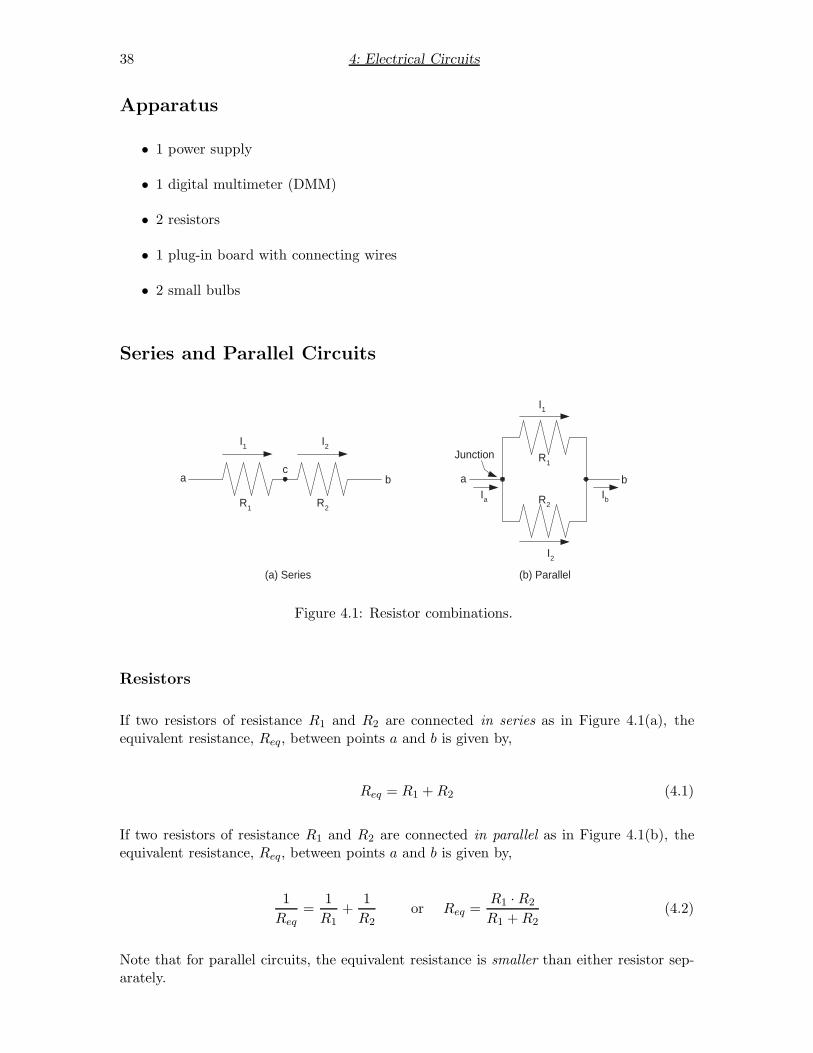
Figure 4.1: Resistor combinations.
Resistors
If two resistors of resistance R1 and R2 are connected in series as in Figure 4.1(a), theequivalent resistance, Req, between points a and b is given by,
Req = R1 + R2 (4.1)
If two resistors of resistance R1 and R2 are connected in parallel as in Figure 4.1(b), theequivalent resistance, Req, between points a and b is given by,
1
Req=
1
R1
+1
R2
or Req =R1 · R2
R1 + R2
(4.2)
Note that for parallel circuits, the equivalent resistance is smaller than either resistor sep-arately.

4: Electrical Circuits 39
Currents in Series and Parallel Circuits
Current is the flow of electric charge (something like the flow of water). There can be noaccumulation of electric charge in a circuit — what comes in must go out somewhere elsein the circuit. Hence in Figure 4.1(a) the charge flowing from a into R1 must flow out ofR1 into R2 and through R2 to b. As a result we can say that the current, I1 through R1
is equal to the current, I2, through R2. In a series circuit the current has no branchingoptions, and hence must be the same throughout the circuit.
Now what about the current in Figure 4.1(b)? In this case, we say that the two resistorsR1 and R2 are connected in parallel. The current from a, Ia, must split into two parts,with part of the current, I1, going through R1 and the balance, I2, going through R2. Toavoid a buildup of charge at the junction where the current divides, the total current outof the junction, I1 + I2, must be equal to the total current into the junction, Ia. That is,Ia = I1 + I2. As we continue through to b, a similar argument applies to junction where thecurrent recombines. The total current into the junction must equal the total current out,that is, I1 + I2 = Ib. Combining these two results leads us to conclude that
Ia = I1 + I2 = Ib (4.3)
Voltages (Potential Differences) in Series and Parallel Circuits
Next we ask, what makes charge flow? Consider the analogy of water flowing in a systemof pipes. Water flows because there is a difference of pressure between two points in thesystem. In electrical circuits, charge flows because there is a potential difference (a voltagedrop) between the points.
Consider the circuit in Figure 4.1(a) again. There will be a current through the resistorR1 if there is a potential difference between the two points a and c. We call the differenceof potential between points a and c (the voltage across R1) Vac. Similarly the potentialdifference between the two points c and b (the voltage across R2) is Vcb. Since the changeof potential from a to c is Vac and the change from c to b is Vcb, then the total change froma to b is
Vab = Vac + Vcb (4.4)
In Figure 4.1(b), there must likewise be a well-defined potential difference between thepoints a and b. Consequently, in a parallel circuit, the voltage drop across the two resistorsmust be the same.
Moving water around a pipe loop requires a mechanical pump (a source of pressure differ-ence). In an analogous fashion, moving electrons around a circuit loop requires a powersource (a source of potential difference). Batteries and power supplies (“battery eliminators”that plug into a wall outlet) are common examples of such source of potential difference.Whatever the name, DC power supplies will have a positive (or “high potential”), terminal(often colored red) and a negative (low potential) terminal (often colored black). The po-tential difference, V , produced by our lab power supplies is adjustable whereas it is fixed

40 4: Electrical Circuits
V V A A Ω FREQ
mACOM
POWER
10AVΩHz
FUNCTION RANGE
TRUE RMS DIGITAL MULTIMETER DM−441B
200 200202
mVΩ kHzV mA k Ω
A MΩ HOLD
NPN
PNPE B C E
ZERO ADJ
1000V
MAX
1000V 750V
2000 10
hFEhFE
Figure 4.2: The DM-441B digital multimeter. When used as a volt/ohm meter, the leftmostinputs (“VΩHz” and “COM”) are used. When used as an ammeter, the bottom inputs(“mA” and “COM”) are used. “COM” refers to common or ground: the low terminal. Thefunction buttons determine the mode of the multimeter: V (voltmeter), A (ammeter), andΩ (ohmmeter). AC modes are denoted with
and DC modes are denoted with . Notethat accurate measurement requires you use the appropriate range: the smallest possiblewithout producing an overscale (a flashing display).
for a charged battery (e.g., a 112
V D cell, 9 V “transistor” battery, 12 V car battery, . . . )The symbol used to represent a power supply is:
V
The positive electrode is the high potential terminal and the negative is the low potentialterminal.
Multimeters
We will use multimeters that can be set in either a current-measuring mode or a voltage-measuring mode. In the current-measuring mode the multimeter is called an ammeter,represented by the symbol
A
and in the voltage-measuring mode, it is called a voltmeter, represented by the symbol
V

4: Electrical Circuits 41
V R
(a)
V R
(b)
V R
(c)
A A
V
Figure 4.3: Simple circuit showing how to connect a multimeter as an ammeter and avoltmeter.
Please note: All meters come with specifications indicating their accuracy. See Table4.1 at the end of this lab for DM-441B multimeter accuracies. Note that the uncertaintydepends on the scale used, thus in addition to the result displayed by the DMM you mustalso record the scale used to properly calculate errors. Alternatively you can get in thehabit of recording every digit displayed by the DMM, as that will also tell which scale wasused and make error calculations easier (since the meaning of “1 dgt” will be clear). If youdo not follow these instructions you will have to repeat your measurements!!!
Now we will put all this information together and build a circuit that will allow us to testEqs. (4.3) and (4.4) experimentally.
Figure 4.3(a) is a simple circuit with a power supply and a resistor. Suppose that we wantto measure the current through the resistor, and the potential difference (voltage drop)across it. We must determine how to place the meters in a circuit when we want to measureeither current or voltage.
• Figure 4.3(b) shows where to place an ammeter to measure the current through theresistor. Note that to measure the current through the wire, we place the ammeter sothat this current must pass (no choice) through the ammeter — hence the ammeterand the resistor are in series in the circuit. In order to measure the current in anexisting circuit, a wire must be cut and an ammeter inserted (bridging the cut sectionof wire).
• Figure 4.3(c) shows where to place the multimeter in voltage measuring mode (volt-meter) to measure the potential difference (voltage) across the resistor. Note that weare measuring the difference of potential between two points — one on either side ofthe resistor. The voltmeter and resistor are parallel to each other in the circuit. Inorder to measure the voltage difference in an existing circuit, simply jump the twolocations with the voltmeter.
In short: Ammeters substitute for a wire (in order to sample the full current). Inserting anammeter into a circuit requires “cutting” a wire. On the other hand, using a voltmeters doesnot require disrupting the circuit; simply connect two locations and measure the potentialdifference.

42 4: Electrical Circuits
Procedure
This lab involves two sets of (unrelated) measurements:
1. You will use resistor color codes (see Appendix) to determine the resistances of two re-sistors. Then, using the multimeter as an ohmmeter, you will measure the resistancesof the two resistors separately and then in series and parallel circuits. The valuesobtained from the color codes and the multimeters should agree within experimentalerror.
2. You will use the multimeter in ammeter and voltmeter modes to measure currentsand voltages in series and parallel circuits (“Kirchhoff’s Rules”).
Measurement of resistances using color codes and an ohmmeter
1. Use the color code listed in Table 4.2 below, to determine the resistance of yourresistors, including an estimate of the uncertainty.
2. Use your multimeter to measure the same resistances. You must set the function toΩ and the range to a range that is larger than the resistance you want to measure.Ask the instructor for assistance. Measure and record the resistances of R1 and R2
separately. Leave room in your data table for the uncertainties.
3. Finally, use the multimeter to measure the equivalent resistances for series and parallelcircuits.
(a) Connect the two resistors in series (Fig. 4.1(a)) and measure their equivalentresistance in series. In your notebook draw a schematic circuit diagram showinghow you connected the ohmmeter to the resistors.
(b) Connect the two resistors in parallel (Fig. 4.1(b)) and measure their equivalentresistance in parallel. (Check that you are using the proper—smallest possible—scale.) In your notebook draw a schematic circuit diagram showing how youconnected the ohmmeter to the resistors.
Measurement of currents and voltages in series and parallel circuits
10 V R 1 R 2
I 1 I 2 I a
Figure 4.4: Two resistors connected in a parallel circuit.
1. Prepare the circuit shown in Fig. 4.4. DO NOT turn on the power supply until thecircuit has been checked by the lab instructor. Ask the lab instructor to explain the

4: Electrical Circuits 43
operation of the power supply and learn how to adjust it to get the 10 V potentialdifference needed for these measurements.
2. Use Ohm’s law to make rough calculations of the current you expect in the circuit.When using the multimeter in current measuring mode you must set the range to avalue higher than the current in the circuit to avoid damaging the meter. Plan yourprocedure for measuring the currents, Ia, I1, and I2. You will need to rearrange thewires in your circuit for each measurement so that the ammeter is getting the desiredcurrent. Draw a circuit diagram showing the placement of the ammeter in the circuitfor each measurement. Be sure to use the proper DMM inputs for current (mA), selectthe DC amps function ( A), and insert the meter with the correct “polarity”, that iswith the positive terminal connected to the high potential side of the circuit (positiveof the meter facing the positive of the power supply). Check with the instructorBEFORE turning on any power. Measure and record the three currents.
3. Next, with the ammeter removed from the circuit, measure the voltage across R1 andthe voltage across R2. (Use the proper DMM inputs for voltage, select the DC voltsfunction ( V), and be sure to use the right polarity.) Draw the circuits used tomeasure the two voltages.
10 V R 2
I 2 R 1
I 1
Figure 4.5: Two resistors connected in a series circuit.
4. Prepare the circuit shown in Fig. 4.5. Have the circuit checked by the instructor beforeturning on any power.
5. Measure and record the current through each resistor. Draw a circuit diagram showingthe placement of the ammeter in the circuit for each measurement.
6. Measure and record the voltage across each resistor. Also measure the voltage ofthe power supply. Is this the same as the sum of the voltages across the resistors?Draw a circuit diagram showing the placement of the voltmeter in the circuit for eachmeasurement.
DMM as a component checker
A DMM is often used to check the behavior of various electrical components. As a littleproject, we have put two small light bulbs in the lab. Using only a multimeter, find thefaulty bulb. Explain carefully your procedure, and why you think each bulb is or is notgood.

44 4: Electrical Circuits
Analysis
Resistors
1. Compare the color code values for the resistances of R1 and R2 with your DMMmeasured values. Are they the same within the manufacturer’s tolerance and theaccuracy of the meter used? Make a table of the color code values and your ownmeasurements.
2. Using the DMM measured values of R1 and R2, calculate the equivalent resistance forthe resistors connected in series and in parallel. Compare these values with your DMMmeasured values. Do they agree within the accuracy of the meters? Use Appendix3 as a guide to finding the uncertainty in the equivalent resistance of two resistorsconnected in parallel and Appendix B Eq. B.5 for resistors connected in series.
Currents and Voltages
1. For the parallel circuit, Fig. 4.4, does Eq. (4.3) hold within the accuracy of the meters?Explain.
2. Were the voltages across the parallel resistors the same?
3. For the series circuit, Fig. 4.5, does Eq. (4.4) hold within the accuracy of the meters?Explain.
4. Were the currents through series resistors the same?
5. What do your data tell you about the current drawn by two resistors when connectedin series compared to when they are connected in parallel?

4: Electrical Circuits 45
Appendix 1 — Multimeter Uncertainties
Most meters have accuracies specified by the manufacturer. Table 4.1 reproduces the speci-fications for the DM-441B multimeter provided by its manufacturer. Note that the accuracydepends on the function, and sometimes on the range. Your instructor will have the specifi-cations for any other meters that we may use. In the table, the letters “dgt” stand for leastsignificant digit — the right-most digit on the display; “4 dgt” means 4× whatever a 1 inthe right-hand digit (and zeros everywhere else) would correspond to. (In the below table“Resolution” is the same thing as “1 dgt”.) Note that the value of 1 dgt always changeswith the range, so you need to record both the range and the value when you take data.Some of the expressions are a bit complex. It may help to use a spreadsheet to calculatethem.
Table 4.1: DM-441B Multimeter Resolution and Accuracy
Function Range Resolution Accuracy
Resistance 200Ω 0.01Ω ±(2% + 5 dgt)2 KΩ 0.1Ω ±(0.2% + 2 dgt)20 KΩ 1Ω200 KΩ 10Ω2000 KΩ 100Ω ±(0.5% + 2 dgt)20 MΩ 1 KΩ
DC Voltage 200 mV 10µV ±(0.1% + 4 dgt)2 V 100µV20 V 1 mV200 V 10 mV1000 V 100 mV ±(0.15% + 4 dgt)
DC Current 2 mA 0.1µA ±(0.5% + 1 dgt)20 mA 1µA200 mA 10µA2000 mA 100µA
10 A 1 mA ±(0.75% + 3 dgt)
AC Voltage 200 mV 10 µV ±(0.5% + 20 dgt)(45 Hz – 1 kHz) 2 V 100 µV
20 V 1 mV200 V 10 mV750 V 100 mV ±(1% + 20 dgt)
Examples: A resistance reading of 71.49 Ω (on the 200 Ω scale) has an uncertainty of:71.49×2%+5 dgt = 1.43+.05 = 1.48 ≈ 1.5 Ω. A DC voltage reading of 6.238 V (on the 20 Vscale) has an uncertainty of: 6.238× 0.1% + 4 dgt = .0062 + .004 = .0102 ≈ .010 V. An ACvoltage reading of 6.238 V (on the 20 V scale) has an uncertainty of: 6.238×0.5%+20 dgt =.0312 + .020 = .0412 ≈ .041 V.

46 4: Electrical Circuits
Appendix 2 — Resistor Color Codes
Resistors have colored bands on them to specify their resistance. The colored bands aroundthe body of a color-coded resistor represent its value in ohms. These colored bands aregrouped toward one end of the resistor body. Starting with this end of the resistor, the firstband represents the first digit of the resistance value; the second band represents the seconddigit; the third band represents the number by which the first two digits are multiplied.A fourth band of gold or silver represents a tolerance (or uncertainty) of ±5% or ±10%respectively. The absence of a fourth band indicates a tolerance of ±20%. The physical sizeof a resistor is related to its power rating. Size increases progressively as the power rating isincreased. The diameters of 1/2 watt, 1 watt, and 2 watt resistors are approximately 1/8”,1/4”, and 5/16” respectively.
Color 1st digit 2nd digit Multiplier Tolerance
black 0 0 1 —
brown 1 1 10 —
red 2 2 100 —
orange 3 3 1000 —
yellow 4 4 10,000 —
green 5 5 100,000 —
blue 6 6 106 —
violet 7 7 107 —
gray 8 8 108 —
white 9 9 109 —
gold — — 0.1 5%
silver — — 0.01 10%
First digit
Second digit
Multiplier
Tolerance
Yellow = 4
Violet = 7
Orange = 1000
Silver = + 10%
47,000 ohms =
47 K
Red = 2
Red = 2
Green = 100,000
22 x 100,000 ohms =
2.2 M
No band = + 20%
Table 4.2: Resistor Color Code
Appendix 3 — Finding the uncertainty in the equivalent resistance of two re-sistors in parallel
1. We start with our measurements: R1 ± δR1 and R2 ± δR2.
2. The equivalent resistance is of course
1
Req=
1
R1
+1
R2
.

4: Electrical Circuits 47
3. We define a new variable u ≡ 1/R, in terms of which the above equation becomes
ueq = u1 + u2.
4. We calculate the uncertainties in both u’s using the techniques you learned in Physics191:
δu
u=
δR
Rusing the form R = K/a.
In our case,
δu = uδR
R
δu =1
R
δR
Ror
δu =δR
R2
Use this result to find δu1 and δu2.
5. It is now easy to find δueq =√
(δu1)2 + (δu2)2 (since the generic form is R = a + b)
6. Finally, to find δReq , we do the same process in reverse: Follow the reasoning above,and persuade yourself that
δReq = R2eq δueq.
Use this procedure to find δReq from δR1 and δR2. A spreadsheet may help to make thesecalculations more organized and less tedious! It’s even easier in Mathematica.

48 4: Electrical Circuits

5. RC Circuits
Purpose
The purpose of this experiment is to investigate circuits with time-varying signals, whichalmost always involve capacitors.
Introduction
Ideally the current through a resistor responds instantaneously to changes in applied voltage,instant by instant following Ohm’s Law: I = V/R. This is not true of capacitors: theresulting current flow through a capacitor depends on history and time, not just the appliedvoltage. This time lag between voltage and current is put to use in most every circuit whichhas changing voltages or currents (“AC”). For example, capacitors are used in ‘filtering’AC signals (e.g., boosting the bass—low frequency—but not the treble), in fully electronicsound sources (synthesizer, audio oscillators), and in tuned circuits used to select TV orradio frequencies.
The rate at which a capacitor charges or discharges is governed by an exponential law. Inthis experiment, we will investigate the behavior of capacitors as they charge and discharge.Since we expect this behavior to involve exponential functions, the data analysis techniquesdescribed in the Appendices to the Physics 191 laboratory manual will be useful—youshould review them as needed.
Theory
Figure 5.1 shows an idealized circuit for studying the charging and discharging of a capacitor.
Charging: We first consider the case when the switch is put in position 1 to charge thecapacitor. Applying Kirchhoff’s first rule to this circuit yields:
V0 − IR − Q
C= 0, (5.1)
49

50 5: RC Circuits
R
C−Q−Q
+QV0+
1
2
Figure 5.1: Simple charging/discharging circuit for a capacitor.
where V0 is the emf supplied by the power supply, Q the charge stored on the capacitorplates, and I the current in the circuit. Note that:
I =dQ
dt, (5.2)
and hence Eq. (5.1) can be written:
V0 − RdQ
dt− 1
CQ = 0. (5.3)
This equation is a differential equation that can be solved for Q to give
Q = CV0
[
1 − exp
(
− t
RC
)]
(5.4)
where we have assumed that the charge on the capacitor at t = 0 was zero. We can usethis equation to find both the voltage drop across the capacitor, VC and the current in thecircuit as functions of time. Consider first the voltage drop. If we divide Eq. (5.4) by thecapacitance C and use the definition of capacitance C = Q/V , we obtain
VC = Q/C = V0
[
1 − exp
(
− t
RC
)]
. (5.5)
Now consider the current: If we take the derivative of Eq. (5.4) with respect to time, weobtain
I =dQ
dt=
V0
Rexp
(
− t
RC
)
(5.6)
which allows us to find the voltage across the resistor using Ohm’s law: VR = IR.
Consider Eq. (5.4) first: It says that if we close the switch in position 1, the charge on thecapacitor, Q, will increase with the time t. In the limit as t → ∞, exp (−t/RC) → 0 and
Q → Q∞ = CV0, (5.7)
which is the final charge on the capacitor. Figure 5.2(a) shows Q plotted as a function oftime — Q approaches Q∞ asymptotically. Similarly, Eq. (5.5) shows that the voltage dropVC across the capacitor approaches V0 in the limit.
In all of these equations, the rate at which the capacitor charges is governed by the factor(t/RC), that is RC sets the scale for time variation. We find it useful to define the timeconstant τ ≡ RC.

5: RC Circuits 51
t
Q∞
Q = Q∞ (1 − e−t /τ)
t1=τ
τ = R C
Q1=.63 Q∞
Q
(a) Charge, Q, as a function of time.
t
I0
I = I0 e−t /τ
I1 = .37 I0
t1=τ
τ = R C
I
(b) Current, I , as a function of time.
Figure 5.2: Charging capacitor: charge and current as a function of time.
Exercise: Show that RC has dimensions of time by working out the dimensionsof both R and C in terms of the fundamental quantities mass, length, time, andelectric charge. Note that we could have predicted this result in advance, since theargument of an exponential must be dimensionless.
To see the significance of the time constant, consider the following argument: If t1 = τ = RCis put into Equation 5.4, we obtain:
Q1 = CV0 [1 − exp (−1)] = CV0
(
1 − 1
e
)
, (5.8)
Thus,
Q1 = Q∞
(
1 − 1
e
)
≈ 0.63 × Q∞ (5.9)
This result says that at time t1 = RC the charge is within 1/e of its final value Q∞.
Note that if t = τ = RC is used in Equation 5.6 we get:
I1 =V0
Rexp (−1) =
1
e
(
V0
R
)
=1
eI0 ≈ 0.37 × I0. (5.10)
Figure 5.2(b) shows I plotted as a function of t (Equation 5.6). I approaches zero asymp-totically as t → ∞. The current has its maximum value, I0, initially (i.e., just after theswitch is placed in position 1) and thereafter declines exponentially. Note that I0 = V0/R.
Discharging: Consider next the case when the capacitor is discharging. Suppose thatthe capacitor has a charge Q0 on it and the switch is moved to position 2 (Figure 5.1),Kirchhoff’s first rule yields:
IR − Q
C= 0. (5.11)
But I = dQdt , so Equation 5.11 becomes:
RdQ
dt− 1
CQ = 0. (5.12)
The solution to this differential equation is:
Q = Q0 exp
(
− t
RC
)
(5.13)

52 5: RC Circuits
C
R
VR
VC
toS
cop
e
Fu
nct
ion
Ge
ne
rato
r
ground
Figure 5.3: Experimental setup to determine the time constant of an RC circuit.
where we have assumed the capacitor has charge Q0 initially. If we again apply the definitionof capacitance C = Q/V to this result, we find that the voltage drop across the capacitoras a function of time is
VC = V0e−t/τ (5.14)
where we have substituted for the time constant τ = RC. If we again consider the timet1 = τ , then:
V1 = V0 e−1 ≈ 0.37 × V0. (5.15)
Hence in a time equal to the time constant, the capacitor discharges to a voltage which is1/e of its initial value. Note, also, that if we differentiate Equation 5.13 with respect totime we get the discharging current:
I =dQ
dt= − Q0
RCe−t/τ . (5.16)
The negative sign tells us that it has the opposite direction as the charging current, andsince C = Q0/V0:
I = −V0
Re−t/τ = −I0 e−t/τ , (5.17)
where I0 = V0/R is just the initial current. Again, if desired, the voltage across the resistorcould be found using Ohm’s law: VR = IR.
How can we measure the time constant in the laboratory? The theory indicates that, if wecould measure Q, V , or I as a function of time, the time constant τ could be determinedby fitting the theoretical equation (for Q(t), V (t), or I(t)) to the experimental data. Eitherthe charging or discharging of the capacitor, or both, could be used. The circuit shown inFigure 5.3 will allow you to measure the voltage, VC , across the capacitor; or if the capacitorand resistor are interchanged, you may measure on the oscilloscope the voltage across theresistor, VR. (Why is it necessary to interchange these components, rather than just movethe oscilloscope leads?) If you measure VC , then Q may be obtained from Q = VCC. Ifyou measure VR then I is obtained from I = VR/R. In this lab you will measure VC as afunction of time, and then fit the resulting data to the expected exponential form Eq. 5.14.
To simulate the situation developed in the theory above the function generator should be setto the square wave mode. A square wave can be thought of as a d.c. voltage that is turnedon and off at regular intervals. Thus, the square wave alternately charges the capacitor,and allows it to discharge. You will simultaneously observe both the square wave and VC
by using the both channels of the oscilloscope.

5: RC Circuits 53
The oscilloscope will also be used to measure the voltage across the resistor. If you are atall hazy on how to use the oscilloscope, you should review the write-up for the oscilloscopeexperiment you performed earlier this semester.
Procedure
Qualitative Analysis
1. Set up the circuit. Initially set the resistance R ∼ 10 kΩ, and capacitance C ∼0.1 µF. Connect the output from the function generator to the CH 1 scope input andVC from your circuit to the CH 2 input. Have your lab instructor check your circuit.
2. Recall the oscilloscope’s Setup 1. (See the digital oscilloscope lab, page 27, for details.)At this point the scope will only be displaying CH 1. Hit the CH 2 menu button sothe scope will display both channels.
3. Set the function generator to the 200 Hz frequency range, an amplitude of about50%, and a square wave ( ) function. Hit autoset on the scope. Check to see thatthe scope is displaying a square wave and that the scope’s display responds properlywhen you adjust the function generator’s frequency and amplitude knobs. Notethat you can use the vertical position knobs to locate the traces anywhere you wanton the display. (For the below Quantitative Analysis, we will want them to exactlysuperimpose, but that may make viewing/sketching difficult.) Start with identicalvertical scales (volts/div the same for CH 1 and CH 2), but if CH 2 looks flat, blowup that scale so you can see its behavior—autoscale can help!
4. Observe the effects of changing the function generator frequency, f , as well as thevalues of R and C. (Keep the resistance in the range: 100 Ω < R < 100 kΩ.)
5. Let T = 1/f be the period of the square wave. Make careful sketches in your notebookof the wave forms you obtain for T ≫ RC and T ≪ RC. (Adjust scope scale factorsto maintain a meaningful plot of the signal: the signal should be at least 3 divisionshigh with at most two cycles on screen.) Be sure to give the values of T , R, C, andRC for each sketch and record each axis scale. Give a careful explanation of the shapeof each waveform. (Note: 10 ≫ 1. If the disparity between T and RC is too large youmay obscure what’s going on.)
6. Rearrange your circuit to measure VR. Note that since the scope measures voltagerelative to ground, we must arrange the circuit so that one end of the resistor is atground and the other end is attached to the scope probe. Thus the desired circuit willhave resistor and the capacitor swapped compared to the circuit in Figure 5.3. Theeasy way to swap the R and C components is actually to just reverse the leads fromthe function generator. . . Can you see why this works?
For the same conditions you used in part 5, make sketches of the wave forms observed.
Quantitative Analysis
Now, we will take data for VC , the voltage across the capacitor, as a function of time. Ifthese data are consistent with an exponential, we should be able to find the time constant

54 5: RC Circuits
τ from the B value of the fit. (Of course you will want to compare the value of τ calculatedfrom the fit to that suggested by theory: RC.)
First, be sure that you rearrange the circuit so that you are again measuring VC , the voltageacross the capacitor.
Find values of R and C that result in a nice dis-charging pattern on the oscilloscope. (triggerSlopeFalling may be helpful.) Use the horizontalposition knob to move the start of the discharge cy-cle to the middle of the first division of time, i.e.,near the left hand side of the screen. (The end of thedischarge cycle should be off the rhs of the screen.)
Vo
τ
.37 Vo
With CH 1 and CH 2 on the same scale and positioned with the same zero value, the CH 2trace should have discharged to essentially the CH 1 value by the right hand side of thedisplay. You will need to fiddle a bit with the scope scales (both volts/div and sec/div)and positions (both horizontal and vertical), the values of R and C, and the functiongenerator frequency to achieve a proper display.
When you have achieved a proper display, hit the cursor button in the scope’s menu area.In the action area select: TypeVoltage and SourceCH2. Line up the bottom cursor (usingthe position knobs) with the final discharge voltage V∞ (the bottom of the CH 1 squarewave). Record the numerical value corresponding to V∞. To measure VC , move the othercursor so that it crosses the CH 2 curve at the desired time and record Delta as VC .
Make a table reporting values of time and VC at every full-division (vertical line) time divi-sion. In an adjacent column record the vertical scale used when the voltage was measured.Leave room for a column for the error in VC (δV ). (The formula for the uncertainty in volt-age can be found in the manufacturer’s specifications recorded on page 36.) As the voltagedifference gets smaller you must change vertical scales (maintaining the equality betweenthe CH 1 scale and CH 2 scale). This will require vertically repositioning the graphs andthe cursors to accommodate the changed scale. (Don’t change the horizontal positiononce you’ve started to take data!) Collect 8 or 9 data points (which often requires two orthree scale changes).
Hints for Making Accurate VC vs. Time Measurements
Proper instrument use always requires setting the proper scale (range), which is typically themost sensitive range without producing an out-of-range reading. For scope measurementsyou should change to a more sensitive range if what you’re trying to measure is smallerthan about 3 divisions. Usually such a change is easy: just turn the volts/div knob, butfor this experiment much more is required:
• The CH 1 vertical position must match the CH 2 vertical position, i.e., the zero-location of the two channels must match. In addition, the CH 1 and CH 2 verticalscales must match.
• Initially note the little markers: 1- and 2- on the left hand side of the screen: theymark the location of zero volts for each channel. You can assure zero-location equality

5: RC Circuits 55
by moving these markers (using the position knob in the vertical section of thecorresponding channel) so that they are superimposed. When you turn a positionknob the numerical position of the marker is displayed on the bottom of the screen.Make sure these numerical values match for the two channels!
• Once you enter cursor mode, the position knobs do not move the plots. (Insteadthey move the cursors.) To exit cursor mode, and thus activate the position knobsfor vertical plot adjustment, you must hit either channel’s menu button.
• For the larger time data points, VC approaches its asymptotic value (V∞), and theCH 1 and CH 2 vertical scales must be changed to blow up the ever smaller differencebetween VC and V∞. At these more sensitive scales, the zero-point markers will beoff the top of the screen, and so you must line them up just using the numerical valueof the vertical position displayed on the bottom of the screen when the channel’sposition knob is turned.
• There is a limit to selecting a properly sensitive scale: while the zero level may be off-screen it may not be more than 10 divisions high. You will typically reach this limitafter 2–3 scale changes and then be forced to make relatively high-error measurementsfor the remaining points with Delta corresponding to a few divisions or even a fractionof a division.
• Record the value of the cursor marking V∞. As you change vertical scales this numer-ical value should be the same! (But see following.)
• The V∞ produced by the function generator may not be exactly constant, in whichcase you should measure its value at the same vertical grid line (time) as CH 2 VC .
• Each time you record a voltage measurement, also record the scale in use for thatmeasurement; the scale is required to calculate the error! (The scale isdisplayed at the bottom of the screen.)
• Use of a spreadsheet will make calculating δV easier.
• Be sure to accurately measure voltages at the grid time divisions as we will be ne-glecting the uncertainty in time.
Lab Report
Use WAPP+ to fit an exponential function to your voltage vs. time data. Produce a normalplot and a semi-log plot. Attach these plots along with the fit report in your lab notebook.Comment on whether your data are indeed consistent with exponential behavior.
Calculate value of τ and its error using the computer fit B value and its error. (Sinceτ = −1/B, what is the uncertainty in τ?) Calculate the expected value of τ (and its error)from the readings on the variable resistor and capacitor. (The readings on the variableresistors are good to ±10% and the readings on the variable capacitors are good to ±20%.What is the uncertainty in the product RC?) Within the limits of error, are these τ equal?Make a nice table properly reporting both numerical values for τ (including error and units).

56 5: RC Circuits
Critique of the Lab
Comment on the clarity of the Lab Manual, the performance of the equipment, the relevanceof the experiment, etc. This critique will help us improve the lab experience.

6. Ohmic & Non-Ohmic CircuitElements
Purpose
To extend your knowledge of DC circuits to nonlinear circuit elements.
Introduction
The purpose of this lab is to extend your knowledge of DC circuits to include circuit elementsfor which the relationship between current and voltage is not a simple linear function.Such circuit elements are called non-linear or non-ohmic devices. Non-ohmic components,particularly those involving semiconducting PN junctions, are critical to the operation ofmost any modern electronic device. (Before the invention of transistors in 1947, vacuumtubes were the non-linear components of choice.) In 1939 electrical engineers Bill Hewlettand Dave Packard made innovative use of the non-linear behavior of a light bulb in designingthe Model 200A audio oscillator—the first product of the Hewlett-Packard Company.
In this experiment we will investigate three common circuit elements to investigate linear(ohmic) and two types of non-linear behavior. We will use digital multimeters (DMM) torecord how the current, I, through a circuit element depends on the voltage drop, V , acrossit. We will go on to use techniques of graphical analysis that you learned in Physics 191 toinvestigate the functional relationship between I and V for a resistor, a diode, and a lightbulb. You may find it useful to review the Appendices in the Physics 191 lab manual asyou perform this analysis.
Apparatus
• 1 power supply
• 2 digital multimeters
• 1 circuit bread-board
• 1 resistor: 2.7 kΩ
• 1 diode (2N3904 transistor with collector and base wired together)
57

58 6: Ohmic & Non-Ohmic Circuit Elements
• 1 light bulb
Theory
Ohm’s law states that the current flowing through a circuit element is proportional to theapplied voltage:
V = IR, (R is a constant) (6.1)
The proportionality constant, R, is called the resistance of the circuit element and is in-dependent of I and V . Circuit elements that obey this relationship are called linear orohmic. Although there is no device that displays perfectly ohmic characteristics, manycircuit elements are nearly ohmic over a wide range of currents and voltages.
In general, circuit elements display non-linear behavior. For such circuits, the current isnot directly proportional to the applied voltage; V/I ≡ R is not a constant. In such caseswe convert Ohm’s Law into a definition of a non-constant resistance:
R ≡ V
I(6.2)
NOTE: Ohm’s Law states that for many materials V/I is a constant—whereas for non-ohmic materials V/I changes along with the current and voltage. Equation (6.2) is notequivalent to Eq. (6.1), even though they look alike. Equation (6.1) indicates that for alinear circuit element a plot of I versus V yields a straight line. Equation (6.2) is a definitionof a (potentially non-constant) R. For non-ohmic materials a plot of I versus V will showsome sort of curvature. If the graph is a curve (i.e., if the slope changes) it is sometimesuseful to define a dynamic resistance, r:
1
r≡ dI
dV(6.3)
Procedure
Examine the apparatus for this experiment. With the assistance of the lab instructor,become familiar with the operation of the multimeters and power supply. Always havethe lab instructor check your circuits before turning on the power supply! Notethat you will make graphs of current on the y-axis vs. voltage on the x-axis . If the graphis a straight line, the slope of this graph (a constant) will be the inverse of resistance, i.e.,1/R. If the graph has curvature, the slope of the graph varies with V and is 1/r.
Linear Circuit Elements
Build the circuit shown in Figure 6.1 using the circuit breadboard and banana plug con-nectors. You will measure current through the resistor as a function of voltage across theresistor for voltages up to 9 V. (Such measurements define what is called the IV character-istic of a circuit element.) Use the color code on the resistor (page 46) to find the resistance

6: Ohmic & Non-Ohmic Circuit Elements 59
R
A
V
P.S.
Figure 6.1: Linear circuit. Here P.S. stands for the power supply.
of the resistor, and then use Ohm’s law, Eq. (6.1) to find the maximum current expectedfor this range of voltage. Set the initial range on each multimeter to accommodate themaximum current and voltage. Be sure to have your instructor check these range settingsbefore you proceed. When the circuit is ready, make a table listing the current and voltagedata and the errors associated with your measurements.
NOTE: The accuracies of the DM-441B multimeters are given on page 45. For this DMM(and most any meter) the accuracy depends on the range, so you must record the rangeused in addition to the value to calculate the error. Of course, you should always use anymeter on its most sensitive scale that avoids an out-of-range reading. (On a DM-441B, anout-of-range measurement is displayed as a flashing display.) In analyzing your data it willbe helpful if you record every digit (even trailing 0s) displayed on the DMM.
Measure the current as the voltage is varied from .5 V to 9 V; record at least a dozen well-spaced data points. (Why shouldn’t you use 0 V as a point?) Plot the current I (on they-axis) versus the voltage V (on the x-axis). The plotted data points should vary smoothly.If any data points look suspicious, recheck them while the circuit is still intact. When youare satisfied that the data accurately reflect the experimental conditions, turn down thevoltage and shut off the power supply to prepare for the next part of the experiment.
Non-Linear Circuit Elements
Diode
Add a diode to your circuit, as shown in Fig. 6.2(a). The symbol
is used to represent a diode and the arrow indicates the direction of the current (positivecharge). In this experiment, we are using a transistor with two terminals wired together asthe diode—it turns out that its behavior is closer to that of a theoretically “ideal” diodethan the inexpensive diodes used in power supplies.
You should take data from about 0.5 V (lower if your ammeter can handle very low cur-rents) to about 0.8 volts, and measure using at least 10 voltages, approximately equallyspaced, within this range. You will need to frequently adjust the range of the ammeter to

60 6: Ohmic & Non-Ohmic Circuit Elements
A
V
P.S.
R
(a) Nonlinear circuit with a diode.
A
V
P.S.
(b) Nonlinear circuit with a light bulb.
Figure 6.2: Nonlinear circuits.
accommodate this current, which should grow rapidly as the voltage is increased. Haveyour instructor check the circuit before turning on the power supply — it canbe tricky to be sure the polarity is correct. As before, measure, record and plotthe IV characteristics for the diode. Again: when the currents are small, use the lowerranges on the multimeter to reduce your experimental uncertainty—but remember that theuncertainties do depend on the ranges, so you must record the range used in addition tothe DMM reading.
Next we will investigate the effects of changing the direction of the current flow throughthe diode. Reverse the direction of the diode in the circuit and observe the current as thevoltage is increased to about 1 V. You need not record data points during this part of theexperiment, but note your observations of the circuit’s behavior in your lab notebook. Asalways, turn down the voltage when done and shut off the power supply.
Light Bulb
We will now investigate the IV characteristics of a light bulb using the circuit shown inFig. 6.2(b); replace the diode with the bulb.
Do not exceed the voltage rating of the light bulb—if you aren’t sure, stop at the point thebulb seems to be extremely bright. Collect IV data following a procedure similar to thatused for the diode and resistor. Try to collect data using a wide range of voltages, with,say, Vmin ∼ 1
10Vmax When you have completed taking data, turn down and shut off all
equipment.
Analysis
Using WAPP+ (Goggle “wapp+” to find it or use LINFIT) analyze the three sets of currentvs. voltage data. There will be uncertainties in both voltage and current, so be sure youcalculate error in both the x and y coordinates. (Show sample calculations or self-documentyour spreadsheet!) Attach in your notebook the fit reports and five plots (resistor: normal,

6: Ohmic & Non-Ohmic Circuit Elements 61
diode: normal and semilog, bulb: normal and log-log).
1. Resistor: Use the computer data analysis program to determine the resistance andits uncertainty. Comment on the quality of the least-squares fit. Does your resultagree with the color code resistance value1 to within the specified resistor tolerance?
2. Diode: Solid state physics predicts that an ideal diode will obey an exponentialrelationship:
I = I0 exp
(
eV
kT
)
(6.4)
where e = 1.602 × 10⁻¹⁹ C is the absolute value of the charge of the electron,k = 1.3805 × 10⁻²³ J/K is Boltzmann’s constant, and T is the absolute tempera-ture (in Kelvins). Fit your data to an exponential and use B to find the “theoretical”temperature (with an error). Measure the actual temperature in the lab, and see ifthe result of your least-squares fit is consistent with this result, within experimentaluncertainty. Don’t be too surprised if there is a mismatch: real diodes are differentfrom ideal diodes!
3. Bulb: Very approximate theory suggests a power law relationship between I and V :
I = AV 3/5 (6.5)
Fit your data to both a power law and one of the other optional functional forms.Which one works best? (Why?) Does the better functional form actually produce agood fit? (Explain!) Compare the computer-fit power to crude theory’s value of 3
5.
In your lab report, qualitatively discuss the effects of varying the voltage across thesedevices.
Critique of the Lab
Comment on the clarity of the Lab Manual, the performance of the equipment, the relevanceof the experiment, and your pleasure or displeasure with the experiment. Please be honest.This critique will not affect your grade, and serves to help us improve the lab experience.
1see Table 4.2 page 46

62 6: Ohmic & Non-Ohmic Circuit Elements

7. e/m of the Electron
Purpose
In this experiment you will measure the charge-to-mass ratio e/m of the electron. Anotherimportant purpose of the experiment is to enhance your understanding of the use of electricand magnetic fields to control beams of charged particles. The production and control ofa beam of charged particles (electrons or ions) is fundamental to the operation of particleaccelerators (CERN and Fermilab), electron microscopes, mass spectrographs, televisions,microwave ovens, etc.
Introduction
In 1897 the British physicist J. J. Thomson reported on his investigations of “cathode rays”(an electrical current flowing through a vacuum) and concluded that the rays were reallystreams of negatively charged particles (“corpuscles”). This work is usually cited1 as thediscovery of the electron2, the first substructure discovered in atoms3. While a great dealof electrical technology was created without an understanding of the fundamental natureof electricity (e.g., Edison: electric lighting, Bell: telephone), the discovery of the electronallowed the development of much more sophisticated devices like the triode vacuum tube4
(for early radio) and the transistor5 (the basis for all of modern electronics).
Theory
The Ealing e/m apparatus (Figure 7.1) will be used in this experiment. The apparatusconsists of a vacuum tube that encloses an electron gun and an external pair of Helmholtzcoils to produce a magnetic field. Inside the electron gun, electrons are boiled off the
1For example: http://www.aip.org/history/electron/2The word “electron” was actually coined by G. Johnstone Stoney a bit earlier (1891) to denote the unit
of charge found in electrolysis experiments. This idea of a chemical “atom of charge” goes back to the 1830sand Michael Faraday.
3To the Greek philosophers “atoms” were by definition indivisible, so the modern atom with parts (elec-trons and quarks) differs from the the original atom. While “splitting the atom” would be self-contradictoryto Democritus, we retain the term “atom” for the chemical elements even as the search continues for trueatoms: possible substructure inside electrons and quarks.
4Lee DeForest, 19075Shockley, Brattain and Bardeen, 1947
63

64 7: e/m of the Electron
Figure Key
A = Anode of electron gun
B = Space occupied by magnetic field
E = Envelope of vacuum tube
G = Electron gun details
S = Electron beam
H = Helmholtz coils
Z = Heater filament of gun within cathode F = Focusing element of gun
M = Mirror scale to measure beam diameter
W = Lamp to illuminate mirror scale
C, P, J, K, L, N,
R, D =
Various connectors and controls as labeled on front panel
Figure 7.1: Diagram of e/m apparatus.
heated cathode, collimated by the focusing element, and accelerated by the electric fieldproduced by the large voltage difference between the cathode and the anode. Once outsidethe electron gun, the electric field is nearly zero, and the electrons respond to the magneticfield produced by the coils. In general, the force on an electron is governed by the Lorentzrelation:
~F = q(
~E + ~v × ~B)
. (7.1)
In this equation ~F is the force vector on a particle of charge q, moving with velocity vector~v in an electric field, ~E, and a magnetic field, ~B. We denote the charge of an electron byq = −e.
Inside the electron gun, the electrons in the beam gain kinetic energy as they move toregions of lower potential energy (qV ) due to conservation of energy. If the acceleratingvoltage is V the following relationship gives the kinetic energy of the electrons as they leavethe gun:
eV =1
2mv2. (7.2)
If the electron beam is directed with velocity perpendicular to the magnetic field, theelectrons will move in a circular path with the Lorentz force (perpendicular to both ~B and~v) providing the centripetal force. Under these circumstances, the magnitude of the Lorentz

7: e/m of the Electron 65
uniform B field
electron gun
hotcathode
anodeacceleratingvoltage, V
Ele
ctric
Fie
ld, E
rvelocity
magneticforce
Figure 7.2: Schematic diagram of the e/m apparatus. Electrons from the hot cathode areaccelerated by a potential difference V . They enter a uniform B field and move in a circleof radius r due to the magnetic force: q ~v × ~B.
force, given by Equation (7.1), is:F = evB (7.3)
and the magnitude of the centripetal acceleration of the electron is:
a =v2
r, (7.4)
where r is the radius of the circular path. Applying Newton’s second law, F = ma, we have
evB = mv2
r, (7.5)
where m is the mass of the electron. Though we may set up an expression for e/m imme-diately from Equation (7.5), we elect instead to solve for the velocity of the electron herein order to eliminate it from the final equation. Thus we have:
v =erB
m. (7.6)
Now substitute this expression for v into Equation (7.2) and solve for e/m in terms of thelaboratory parameters V , r, and B:
e/m =2V
r2B2. (7.7)
V and r are directly measurable and so we now consider how to find B.
As you may have already learned, the magnetic field B along the axis of a circular coil isgiven by
B =µ0R
2I
2 (R2 + x2)3/2, (7.8)

66 7: e/m of the Electron
where x is the distance along the axis of symmetry of a single current loop of radius Rcarrying a current I. Since there are N current loops in each coil and the loops are arrangedso that their fields add constructively and contribute equally, we have a total field of
B =µ0R
2NI
(R2 + x2)3/2. (7.9)
The Helmholtz coil configuration calls for x = R/2 for each coil. If we substitute this resultinto Eq.(7.9), we obtain a total magnetic field between the coils of:
B =8√125
µ0NI
R. (7.10)
This value for B, derived for the central point on the axis between the Helmholtz coils,closely approximates6 B at the position of the electron beam (which is typically a few cmfrom the center point).
Now substituting the permeability of free space, µ0 = 4π × 10−7 T · m/A; the number ofturns in each coil, N = 130; and the radius of the coils, R = 0.15 m; into Equation (7.10)gives
B =(
7.79 × 10⁻⁴ T/A)
I. (7.11)
Finally, we substitute the expression for B from Equation (7.11) into Equation (7.7) toarrive at an experimentally measurable value of e/m:
e/m =2V
(6.07 × 10⁻⁷) I2r2. (7.12)
Please derive the last two equations as part of your lab report—it would be a good idea todo so before coming to lab. Be sure you include units in your derivation, and in particular,show that the units of e/m are C/kg.
Procedure
PLEASE DO NOT TURN ON ANY POWER SUPPLIES WITHOUT THELAB INSTRUCTOR’S APPROVAL!!!
Possible experimental approaches
In studying Equation (7.12) to determine an appropriate way to make measurements in thelab, we find several approaches are available to us. For example, Equation (7.12) could bewritten as:
V =
[
(
6.07 × 10⁻⁷) (
r2)
(e/m)
2
]
I2. (7.13)
6When typical values of r, x, and R from the Ealing apparatus are used in an exact formula for B off theaxis and compared with (7.10), we are in error by less than 1%. Helmholtz coils are designed to produce alarge region of nearly constant B.

7: e/m of the Electron 67
Now if we keep r constant, a plot of V vs. I2 would yield a slope, S, given by:
S =
(
6.07 × 10⁻⁷) (
r2)
(e/m)
2. (7.14)
Hence,
e/m =2S
(6.07 × 10⁻⁷) r2. (7.15)
Therefore, if we select a value of r and then record a sequence of values of I and V , one canplot V vs. I2, determine the slope, and calculate e/m.
One might also hold the current constant, and measure V as a function of r. Feel free toexplore such alternative approaches.
Error analysis
If you use the procedure outlined above, use the following scheme for error analysis:
• Error in the accelerating voltage V : If you are using the Pasco SF-9585A high voltagepower supply, assume the uncertainty is the least count of the display (that is, 1 volt).(We don’t have specifications for this power supply, but we have checked several ofthem with a multimeter, and this uncertainty looks reasonable to us. Feel free tocheck it yourself!)
• Error in I2: First find the error in I using the table at the end of the ElectricalCircuits experiment, page 45. Then use the techniques developed in the appendicesof the Physics 191 lab manual to find the uncertainty in I2.
• Error in radius r: Estimate this uncertainty from your measurements: How accuratelycan you measure r?
• Assuming the graph of V vs I2 is a straight line, do a fit using errors in both x andy (that is, in both I2 and V ). The fit will give you the uncertainty in the slope S.
• Finally, calculate the uncertainty in e/m taking Eq. (7.15) as your starting point.Note that you will need to use both the uncertainty in the slope, and the uncertaintyin r2, which you should calculate from your estimate of the uncertainty in r using thetechniques you learned in Physics 191.
Detailed experimental procedure
Connect a DC power supply through an ammeter to the Helmholtz coils (check polarity).This ammeter will measure I which should never exceed 2 A. ONLY USE ENOUGH CUR-RENT TO BEND THE ELECTRON BEAM — TOO MUCH CURRENT COULD HARMTHE COILS.
Connect a 6 volt AC source to the electron gun heater (i.e., switch the Pasco SF-9585AAC power source to 6). Connect a high voltage DC source (up to 300 volts) to the electrongun electrodes (note polarity). The power supply voltmeter will measure V across theelectrodes.

68 7: e/m of the Electron
Measurement of the electron orbit radius r is difficult (because the beam is enclosed byglass and hence can not be placed adjacent to the scale) and mis-measurement is common.Parallax error will be avoided only if you carefully align the beam and its reflection in themirrored scale. Measure the left and right sides of the orbit separately and be sure they lieon a diameter (i.e., the mirrored scale should go through the center of the circle). Also, forreasons that you should think about (and record in your notebook), use the outside edgeof the electron beam when determining r.
If you select the approach discussed above you might select r equal to about 4.5 cm andvary V in about 10 volt steps from 150 to 250 volts. CHECK WITH INSTRUCTORBEFORE TURNING THE POWER ON!! Be sure to record all pertinent informa-tion.
Lab Report
1. Tabulate experimental measurements and calculated quantities, particularly the un-certainties.
2. Use WAPP+ (Goggle “wapp+” to find it or use LINFIT) to plot and fit your data.Include the plot and the fit report in your notebook.
3. Answer the following questions:
(a) Why use the outside edge of the electron beam when determining r?
(b) Describe, briefly, how electric and magnetic fields are used to control the particlebeam in a circular particle accelerator.
4. Carefully report the results you found for e/m, including experimental error and units.Compare it to the accepted7 value (1.75882015±0.00000004×10¹¹ C/kg) and discusspossible reasons for any discrepancy.
5. Include any other conclusions, observations, discussion and a lab critique.
7CODATA, 2006

8. Helmholtz Coils
Purpose
In this experiment we shall investigate the magnetic field, B, as a function of position, forthree fairly simple current configurations. We will use the emf induced by a continuouslychanging B (Faraday’s Law) to measure B.
Apparatus
• Helmholtz coils
• function generator
• oscilloscope
• search coil
• apparatus for mounting the search coil on the axis of the Helmholtz coils (benchclamps, heavy rods, and nylon cord)
Theory
One Current Loop
On the axis of a circular wire coil carrying a current I, the magnetic field B is given by
B =µ0NI
2
R2
(x2 + R2)3/2. (8.1)
Here x is the distance along the axis, measured from the center of the coil; R is the radiusof the coil; and N is the number of turns. The direction of B is along the axis of the coil.See your text and class notes for a full derivation and discussion of this result. Our purposehere will be to confirm the x dependence of Equation 8.1.
69

70 8: Helmholtz Coils
Helmholtz Coils
Two identical current loops on the same axis, and separated by a distance equal to theradius of either loop, constitute a set of Helmholtz coils1 . (See Figure 7.1 on page 64 in thee/m experiment in this manual). Such a geometry produces a reasonably uniform magneticfield in the space between the coils:
B =8√125
µ0NI
R. (8.2)
The derivation of this result is long, but not terribly difficult, and may be found in mostintermediate level texts on electricity and magnetism. In this experiment, we will seewhether the field is in fact constant.
Helmholtz Coil with the direction of the current reversed in one coil
If we reverse the direction of the current in one coil, the fields of the two coils will both stillbe along the axis, but in opposite directions. Consequently, instead of adding in the regionbetween the coils to produce a uniform field, they will cancel, and so produce a null field atthe center of the coils. We will attempt to confirm this prediction, and in the process, willuse an important feature of the oscilloscope.
Measurement of B
The Helmholtz coils are described in the e/m lab in this manual. The glass tube used forthe e/m measurement will be removed. Measurement of magnetic fields is always a bitindirect. Unchanging magnetic fields can be measured with a Hall Probe, however thesedevices require calibration and analysis would be confused by the presence of the Earth’smagnetic field. Consequently, in this experiment our field measuring system is designedto be sensitive only to changing magnetic fields. We will drive our coils with a sinusoidalcurrent (using a function generator) so that a sinusoidally varying magnetic field will beproduced:
B = B0 sin ωt (8.3)
Faraday’s Law tells us that a time-varying magnetic field creates an electric field, and soinduces a voltage in any conductor that happens to be present. We will, therefore, detectthe magnetic field by the voltage induced in a small ‘search’ coil. By connecting the searchcoil to an oscilloscope, we will be able to measure the induced emf, and that emf will beproportional to the magnetic field. More precisely, Faraday’s law states that
E = −dΦB
dt, (8.4)
where E is the emf induced in the search coil, and ΦB is the magnetic flux through thesearch coil, defined by
ΦB =
∫
~B · n dA (8.5)
1Named in honor of Hermann von Helmholtz (1821–94).
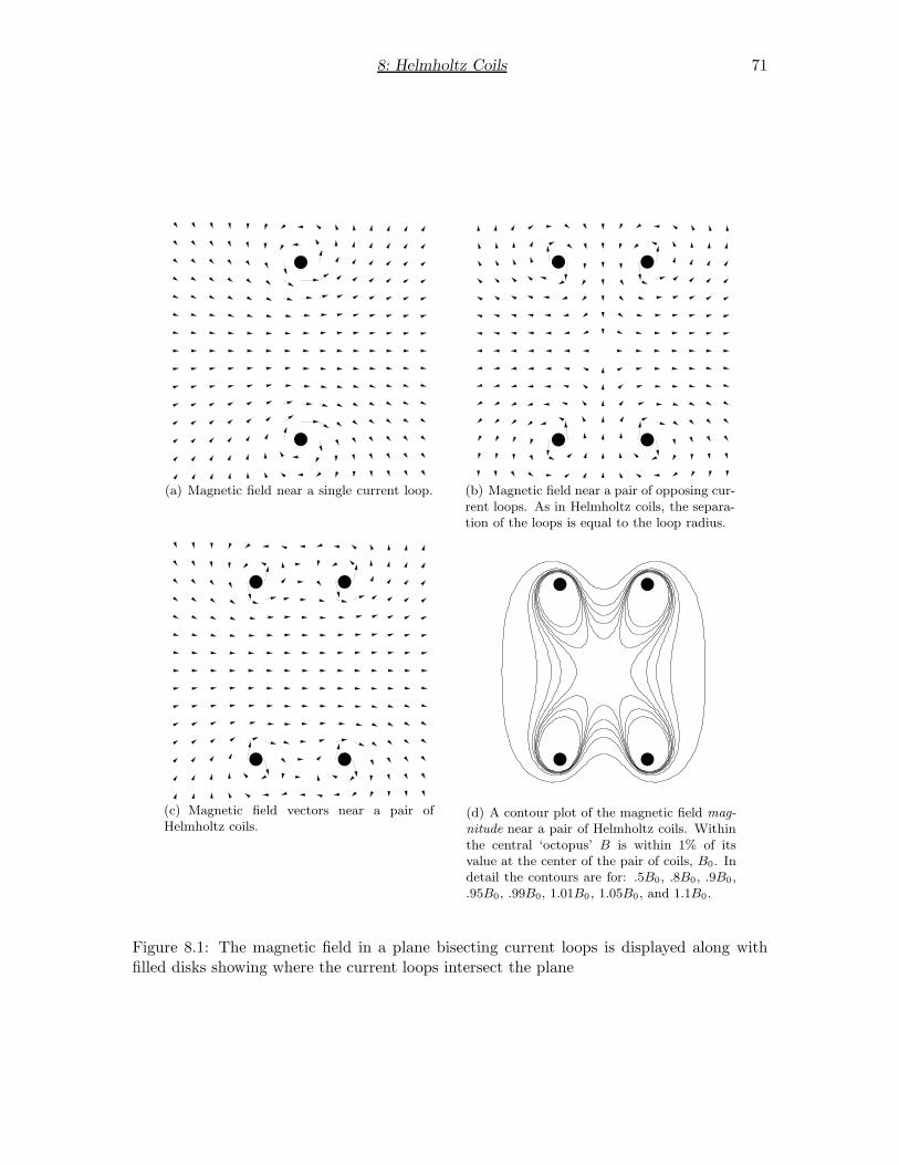
8: Helmholtz Coils 71
(a) Magnetic field near a single current loop. (b) Magnetic field near a pair of opposing cur-rent loops. As in Helmholtz coils, the separa-tion of the loops is equal to the loop radius.
(c) Magnetic field vectors near a pair ofHelmholtz coils.
(d) A contour plot of the magnetic field mag-
nitude near a pair of Helmholtz coils. Withinthe central ‘octopus’ B is within 1% of itsvalue at the center of the pair of coils, B0. Indetail the contours are for: .5B0, .8B0, .9B0,.95B0, .99B0, 1.01B0 , 1.05B0, and 1.1B0.
Figure 8.1: The magnetic field in a plane bisecting current loops is displayed along withfilled disks showing where the current loops intersect the plane

72 8: Helmholtz Coils
where the integral is over the effective area of the search coil. Both ~B and ΦB vary sinu-soidally with time, and hence the induced emf also varies sinusoidally with time:
E = −dΦB
dt= −ω cos ωt
∫
~B0 · n dA (8.6)
and expect to see a sine wave on the oscilloscope. The point to understand here is that theemf induced in the coil is proportional to B0, the amplitude of the magnetic field. (Theproportionality constant between the magnetic field and the voltage displayed on the scopeis not difficult to calculate. However, we will not need it for this lab.)
Procedure
1. Mount the search coil so that it moves along the axis of the coils. Describe yourprocedure. How can you be sure that the search coil is precisely on-axis? Be carefulnot to damage the coil or the cable connection to it.
2. Power up the digital scope and recall the oscilloscope’s Setup 1. (See the digitaloscilloscope lab, page 27, for details.) We will want to measure the Cyc RMS voltageon CH 1. (The measure menu is described in section D, page 30.) Before turning onthe function generator, push in the 20K frequency range button, the sine wave(leftmost:
) function button, and turn the frequency and amplitude knobsto middle positions.
3. Single Coil: Connect the function generator to one of the Helmholtz coils (not both).Place the search coil at the center of the coil, and observe the signal from the searchcoil on the oscilloscope. Adjust the frequency of the function generator for maximumresponse, and record that frequency. You should define the point x = 0 to be at thepoint where the voltage is a maximum—approximately the center of the coil.
Record the voltage of the search coil as a function of distance along the axis of thecoil, using as wide a range of distances as possible. (Take at least 15 data points forvalues of x up to about 1 meter.) Of course, as x is increased the voltage will getsmaller. Change the vertical scale (volts/div) of the oscilloscope when the signalyou’re measuring is smaller than about 3 divisions. (Use of the proper scale allows usto ignore the constant in the complex error formula on page 36; Instead you can usea simple error estimate of 3% for RMS voltage.)
Convert your independent variable to z = x2 + R2 where R = .15 ± .005 m. UsingEq. C.12, the error in z is given by:
δz =√
(2xδx)2 + (2RδR)2 (8.7)
Use a spreadsheet for this calculation! Fit your data to an equation of the formy = AzB . Then see if your results are consistent with Eq. (8.1), which predictsB = −1.5.
Be sure that your results are consistent with a power law, using the appropriate log-log graph. This step often helps correct problems in your procedure, if your data donot initially fall on a straight line.

8: Helmholtz Coils 73
4. Connect both Helmholtz coils and the function generator in series so that the currentin the coils is going in the same direction. Measure the field as a function of positionbetween the coils. Record data out to about x = ±20 cm. (Note that the point x = 0is now defined to be the midpoint on the axis between the two coils.) Present yourresults graphically2. How nearly constant is the field between the coils?
5. Reverse the direction of the current through one of the Helmholtz coils — your in-structor will show you how. See if the field has a sharp minimum at x = 0.
While the Cyc RMS voltage reported by the scope will always be positive it is never-theless possible to confirm that the direction of the field changes half-way between theHelmholtz coils. (That is the voltage should be recorded as negative on one side of thecoil pair.) To observe this effect, trigger the oscilloscope by connecting the functiongenerator’s AUX OUT to the ext trig input of the oscilloscope. Using the scope’strigger menu set SourceExt for external triggering. Be sure you understand howthe external trigger works, and why you need to use it here! Note that with the searchcoil at one side of the coil pair the central peak displayed on the scope will be positive,whereas on the other it will be negative. Record your observations, and explain howthe scope’s display shows that the direction of the field changes at x = 0 (i.e., that Bchanges sign there).
Again, record the field (now with proper sign!) as a function of position between thecoils. Record data out to about x = ±20 cm and present your results graphically.
Lab Report
Carefully summarize your results and answer all questions asked in the lab. Be sure toinclude a discussion of how well your single coil measurements agree with the theoreticalpredictions. As usual, attach your fit report and plots (single coil normal, single coil log-log,Helmholtz coil normal, and anti-Helmholtz coil normal) inside your notebook. Include anycritique you can, commenting on the clarity of the Lab Manual, the performance of theequipment, the relevance of the experiment, etc.
2For plotting without function fitting, follow the link near the top of the WAPP+ page.

74 8: Helmholtz Coils

9. AC Circuits
Introduction
Circuits with time dependent signals (“AC circuits”) are more interesting and useful thancircuits where the voltages and currents are constant. It should be no surprise that goingfrom V (t) = constant to V (t) = anything opens up lots of possible behaviors, but even ifwe limit the voltages and currents to sinusoidal behavior, we have three (rather than justone) parameters to consider— amplitude, A, frequency f , and phase φ:
A sin(2πft + φ) (9.1)
It will save space in writing equations if we define the angular frequency, ω = 2πf .
The three basic AC circuit elements are the capacitor (C), the inductor (L) and the resistor(R). In order to understand the behavior of different AC circuit element combinations, wewill look at one simple yet important circuit, the series LRC circuit, and examine how theamplitude and phase angle vary with frequency.
Theory
First consider the AC behavior of resistors, capacitors, and inductors individually. Forthe purposes of discussion, let the source of emf that we connect these elements across bedescribed by
V (t) = V0 sin(ωt + φ), (9.2)
Resistor: If a resistor is connected across the AC voltage source described by Eq. (9.2),then the resulting current can be determined from the relationship I = V/R. Therefore:
I(t) =V (t)
R=
V0
Rsin(ωt + φ) = I0 sin(ωt + φ). (9.3)
Note that the current has the same frequency f and phase φ as the applied emf and thatthe relationship between the peak voltage V0 and peak current I0 is that given by Ohm’slaw: V0 = I0R. We usually measure AC quantities in root-mean-square (rms) terms, butconverting both peak values to rms leaves the Ohm’s law relationship intact, so Vrms =IrmsR.
75

76 9: AC Circuits
Capacitor: A capacitor is a device whose charge is directly proportional to the appliedvoltage:
Q = CV (9.4)
Recalling that the current is the derivative of the charge with respect to time we can write:
I =dQ
dt= C
dV
dt. (9.5)
If the capacitor is connected across the source of emf described by Eq. (9.2), then theresulting current is
I(t) = Cd
dt(V0 sin(ωt + φ)) = ωCV0 cos(ωt + φ) = I0 cos(ωt + φ). (9.6)
This can be rearranged as:
I(t) = ωCV0 sin(
ωt + φ +π
2
)
. (9.7)
Note that the phase angle for the current in this case is (φ + π/2)—the current leads theapplied voltage by π/2 or 90 (a.k.a. the voltage lags the current by 90: ICE)—and theamplitude is I0 = ωCV0
We can rearrange the sinusoidal amplitudes this equation to look like the Ohm’s law:
V0 = I0
1
ωC= I0 XC (9.8)
where quantity 1/ωC has units of resistance (ohms) and is called the capacitive reactance,XC .
Inductor: An inductor is a device that can store/release magnetic energy. The magneticenergy is a result of the device’s magnetic field which is in turn proportional to the currentflowing through the device. In an AC circuit, this energy is alternately stored and releasedas the current through the inductor causes the magnetic field to increase and decrease. Theinduced emf created by the inductor’s changing magnetic field is E = −LdI/dt. Therefore,when an inductor is connected to the source of emf described by Eq. (9.2) the loop lawbecomes:
V0 sin(ωt + φ) = LdI
dt. (9.9)
Integrating both sides with respect to t gives a relationship involving the current I and theapplied emf:
I(t) = − V0
ωLcos(ωt + φ) =
V0
ωLsin
(
ωt + φ − π
2
)
. (9.10)
Now the phase angle (φ − π/2) indicates that the current lags behind the applied voltageby π/2, a quarter cycle. (Or equivalently the voltage leads the current by 90: ELI.) The

9: AC Circuits 77
R C
L V S
Figure 9.1: LRC series circuit with an AC source.
quantity ωL has units of resistance (ohms) and is called the inductive reactance, XL = ωL.As before we find an Ohm’s Law like relationship between the peak (or rms) quantities:
V0 = I0 ωL = I0 XL (9.11)
LRC Circuit: When these three elements are combined together in one circuit, as inFig. 9.1, the analysis becomes a bit more complicated. To make the algebra as simple aspossible we assume1
I(t) = I0 cos(ωt) (9.12)
and seek the (phase shifted) source voltage as a function of time, V (t), which is consistentwith this choice:
V (t) = V0 cos(ωt + ϕ) (9.13)
To find the phase angle ϕ and the current amplitude I0, we start with the equation derivedfrom the loop law:
V0 cos(ωt + ϕ) − ∆VR − ∆VC − ∆VL = 0. (9.14)
Here ∆VR is just the voltage drop across the resistor,
∆VR = IR = I0R cos(ωt), (9.15)
∆VC is the voltage drop across the capacitor,
∆VC =Q
C=
∫
I dt
C=
I0
ωCsin(ωt) = I0XC sin(ωt), (9.16)
and ∆VL is the voltage drop across the inductor,
∆VL = LdI
dt= −ωLI0 sin(ωt). (9.17)
Thus, the loop law gives the following:
1There is no loss of generality in this choice; it amounts to choosing the instant t = 0 to be when thecurrent peaks.

78 9: AC Circuits
V0 cos(ωt + ϕ) = RI0 cos(ωt) − ωLI0 sin(ωt) +1
ωCI0 sin(ωt)
V0 cos(ϕ) cos(ωt) − V0 sin(ϕ) sin(ωt) = RI0 cos(ωt) −(
ωL − 1
ωC
)
I0 sin(ωt)
= RI0 cos(ωt) − (XL − XC) I0 sin(ωt)
We can conclude:
V0 cos ϕ = RI0
V0 sin ϕ = (XL − XC) I0 (9.18)
Dividing yields the phase angle, ϕ:
tan ϕ =sin ϕ
cos ϕ=
XL − XL
C. (9.19)
Adding the squares yields:
V 20 = V 2
0
(
cos2 ϕ + sin2 ϕ)
=(
R2 + (XL − XC)2)
I20 (9.20)
Solving now for I0 we find that:
I0 =V0
√
R2 + (XL − XC)2. (9.21)
Now we have the expressions for the frequency-dependent amplitude I0 and phase angle ϕof the voltage (relative to the current) in the circuit, in terms of the constant parametersV0, L,C, and R. Note that the frequency f dependence is hidden within the reactances:
XC =1
ωC, XL = ωL, (9.22)
where ω = 2πf .
To simplify a bit more and to help in studying the amplitude and phase functions, definethe impedance of the circuit as
Z =√
R2 + (XL − XC)2, (9.23)
At Resonance
At some frequency it will happen that XC = XL. Clearly, the impedance [Eq. (9.23)] isthen minimized, becoming simply R, and the phase angle [Eq. (9.19)] goes to zero. Since2πf = ω, this frequency satisfies

9: AC Circuits 79
1
2πfC= 2πfL, (9.24)
so the resonance frequency is found to be:
fres =1
2π√
LC. (9.25)
This equation can be rearranged to yield:
C =1
L(2π)2f−2res (9.26)
which is a better match for your fitting equation.
At resonance, Z reaches its minimum value, R, so the current amplitude reaches its maxi-mum value, V0/R. And the phase relationships of the voltages around the circuit at reso-nance are summarized as:
VS = V0 cos ωt
VR = I0R cos ωt
VC =1
ωCI0 sin ωt =
1
ωCI0 cos(ωt − 90)
VL = −ωLI0 sin ωt = ωLI0 cos(ωt + 90) (9.27)
In this form it is clear that the voltage drop across the resistor is in phase with the appliedvoltage, the voltage drop across the capacitor lags the applied voltage by a quarter cycle,and the voltage drop across the inductor leads the applied voltage by a quarter cycle.
Near Resonance
The voltage across the resistor is given by Ohm’s law: VR = I0R, where the current I0 isgiven by Eq. 9.21. Using the expression for reactance Eq. 9.22, we find:
VR =V0R
√
R2 +(
12πfC − 2πfL
)2(9.28)
This equation defines a bell-shaped function displayed in Fig. 9.2.
Procedure
Oscilloscope connections
We want to examine the amplitudes and phase relationships of voltages across the differentcomponents in an LRC circuit. This cannot be done using a DMM. (The DMM does
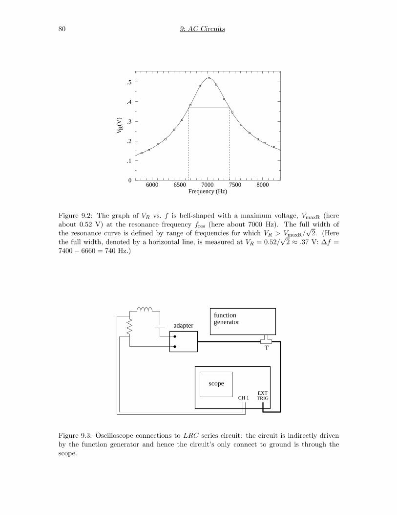
80 9: AC Circuits
6000 6500 7000 7500 8000
.5
.4
.3
.2
.1
0
Frequency (Hz)
V (
V)
R
Figure 9.2: The graph of VR vs. f is bell-shaped with a maximum voltage, VmaxR (hereabout 0.52 V) at the resonance frequency fres (here about 7000 Hz). The full width ofthe resonance curve is defined by range of frequencies for which VR > VmaxR/
√2. (Here
the full width, denoted by a horizontal line, is measured at VR = 0.52/√
2 ≈ .37 V: ∆f =7400 − 6660 = 740 Hz.)
functiongenerator
T
scopeEXTTRIGCH 1
adapter
Figure 9.3: Oscilloscope connections to LRC series circuit: the circuit is indirectly drivenby the function generator and hence the circuit’s only connect to ground is through thescope.

9: AC Circuits 81
not report phase information—just rms voltage—and in addition it cannot measure at the“high” frequencies used in this lab.)
The oscilloscope is a high speed voltmeter and it can display waveforms and hence phaserelationships. However, a scope’s black lead is internally connected to ground and hencecan’t be connected to any other voltage without creating a “short circuit”. This problem canbe avoiding if the circuit being measured has no connection to ground. Then the scope’sblack lead can be connected any place in the circuit—forcing that place to be ground—but creating no ground conflict. Thus your circuit must be driven indirectly through thefunction generator adapter box.
In displaying successively the VR, VL, and VC waveforms on the scope, you must make surethe scope always displays the spot t = 0 in the same location. (Of course, you should alsomaintain the same horizontal scale.) Thus (as in the Helmholtz Coils experiment), you usethe external trigger feature of the scope. Use a T adapter to send the function generator’soutput both to the circuit and to the ext trig input of the scope. Using the triggermenu, select SourceExt . When the input signal is increasing and goes through a valueof zero, the oscilloscope is told to start drawing the trace of the measured signals. Thistriggering point should be in the center of the display and is marked with a little triangleat the top of the display. (Turning the horizontal position knob allows you to move thelocation of the trigger point on the display.)
If the trace of the measured signal starts at zero and is increasing (i.e., looks like a sinewave), then that signal is in phase with the triggering signal. On the other hand if thetrace of the input signal starts at its maximum value and then decreases (i.e., looks like acosine wave), then you know that the input signal leads the triggering signal by 90. Also ifthe input signal starts at its minimum value and then increases (i.e., looks like an invertedcosine wave), then you know that the input signal lags the triggering signal by 90. Externaltriggering is a very powerful tool and is used frequently in all kinds of applications. If youare having trouble, don’t be afraid to ask the lab instructor for help!
1. After turning the scope on, press the save/recall menu button. (See page 27.)Make sure the number 5 is displayed in the Setup box. Press the button next to theRecall box. The message “Setup 5 recalled” should temporarily appear in the lowerleft section of the display and bottom of the display should then read:CH1 20.0mV M 100µs Ext 0.00V
2. Press the trigger menu button. Notice that the slope is set to Rising and the sourceis set to Ext. When you use the autoset feature, the trigger source is reset to CH1;you must then by hand reselect SourceExt.
If you become lost in a series of menus, Setup 5 can always be recalled from thesave/recall menu.
Note that each channel (i.e., input) on the oscilloscope actually has two connections. One,called the pin, is the center conductor of the coaxial cable and is the red (positive) input.The other, called shell or black, is a shield that is wrapped around the central conductorto reduce stray electrical signals (noise). This surrounding shell is grounded—actuallyconnected to the ground in the wall outlet—shielding the center signal wire.
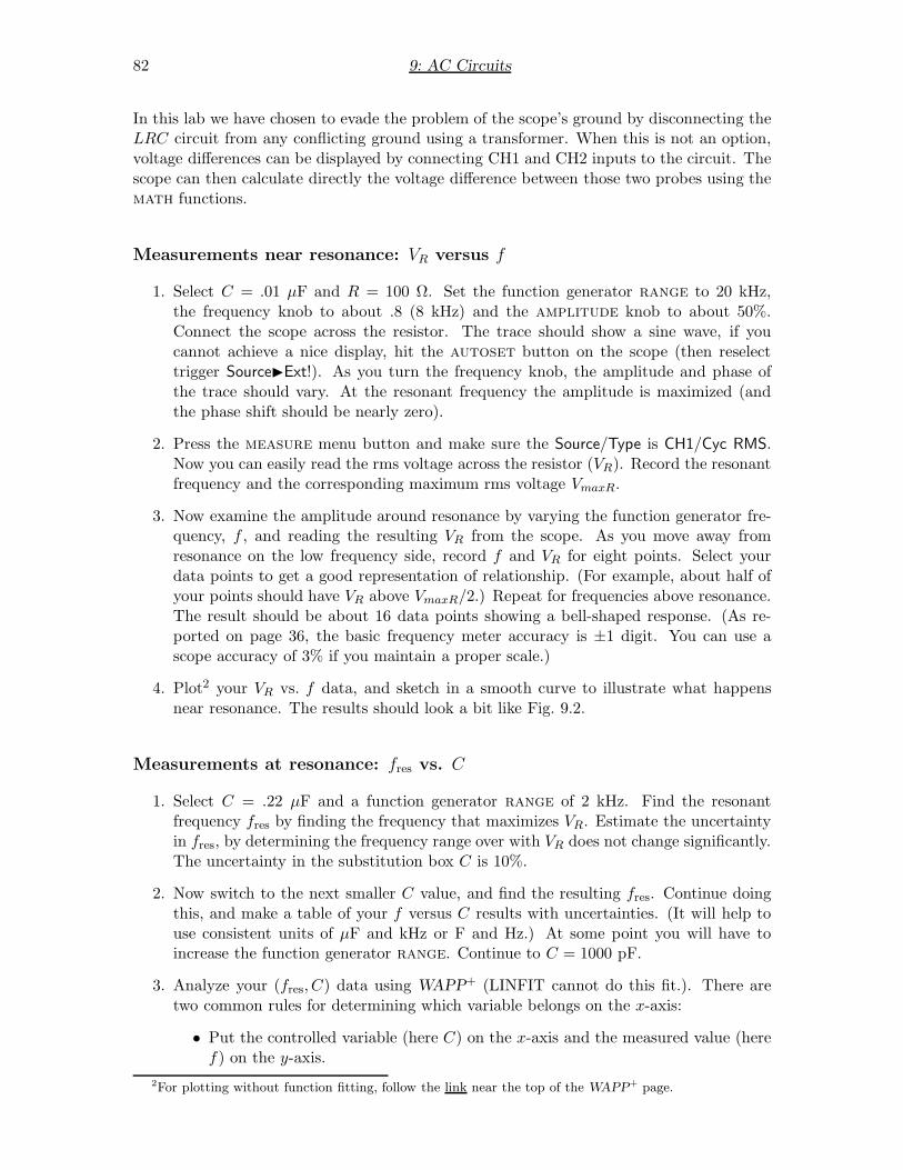
82 9: AC Circuits
In this lab we have chosen to evade the problem of the scope’s ground by disconnecting theLRC circuit from any conflicting ground using a transformer. When this is not an option,voltage differences can be displayed by connecting CH1 and CH2 inputs to the circuit. Thescope can then calculate directly the voltage difference between those two probes using themath functions.
Measurements near resonance: VR versus f
1. Select C = .01 µF and R = 100 Ω. Set the function generator range to 20 kHz,the frequency knob to about .8 (8 kHz) and the amplitude knob to about 50%.Connect the scope across the resistor. The trace should show a sine wave, if youcannot achieve a nice display, hit the autoset button on the scope (then reselecttrigger SourceExt!). As you turn the frequency knob, the amplitude and phase ofthe trace should vary. At the resonant frequency the amplitude is maximized (andthe phase shift should be nearly zero).
2. Press the measure menu button and make sure the Source/Type is CH1/Cyc RMS.Now you can easily read the rms voltage across the resistor (VR). Record the resonantfrequency and the corresponding maximum rms voltage VmaxR.
3. Now examine the amplitude around resonance by varying the function generator fre-quency, f , and reading the resulting VR from the scope. As you move away fromresonance on the low frequency side, record f and VR for eight points. Select yourdata points to get a good representation of relationship. (For example, about half ofyour points should have VR above VmaxR/2.) Repeat for frequencies above resonance.The result should be about 16 data points showing a bell-shaped response. (As re-ported on page 36, the basic frequency meter accuracy is ±1 digit. You can use ascope accuracy of 3% if you maintain a proper scale.)
4. Plot2 your VR vs. f data, and sketch in a smooth curve to illustrate what happensnear resonance. The results should look a bit like Fig. 9.2.
Measurements at resonance: fres vs. C
1. Select C = .22 µF and a function generator range of 2 kHz. Find the resonantfrequency fres by finding the frequency that maximizes VR. Estimate the uncertaintyin fres, by determining the frequency range over with VR does not change significantly.The uncertainty in the substitution box C is 10%.
2. Now switch to the next smaller C value, and find the resulting fres. Continue doingthis, and make a table of your f versus C results with uncertainties. (It will help touse consistent units of µF and kHz or F and Hz.) At some point you will have toincrease the function generator range. Continue to C = 1000 pF.
3. Analyze your (fres, C) data using WAPP+ (LINFIT cannot do this fit.). There aretwo common rules for determining which variable belongs on the x-axis:
• Put the controlled variable (here C) on the x-axis and the measured value (heref) on the y-axis.
2For plotting without function fitting, follow the link near the top of the WAPP+ page.

9: AC Circuits 83
• Put the small error quantity on the x-axis and the large error quantity on they-axis. The 10% error in C is in this case almost certainly larger than your errorestimate for f .
Following this last rule use C = Y and f = X and fit the data to the power lawfunction Y = AXB . In this case Eq. (9.26) requires B = −2, so you must hold Bfixed with that value. You will use the A parameter from the fit to find the inductanceL.
Measurements of phase relationships at resonance
1. Return to C = .01 µF and adjust the frequency for resonance. Reduce the functiongenerator amplitude to approximately 20%. (This frequency and amplitude should bemaintained for the following measurements.) Make sure the scope is set for Externaltriggering. Use the oscilloscope to measure the rms voltage across the resistor. Recordthe rms voltage and make a careful sketch of the waveform. Be sure to record timeand voltage scale factors! (See page 28 if you’ve forgotten where the scale factors aredisplayed. It will be necessary to change the vertical (voltage) scale; do not changethe time scale.) Pay careful attention to the trace around the trigger point (markedwith a triangle at the top of the display).
2. Without changing the order of the oscilloscope leads, move the leads around thecircuit to measure the voltages across the capacitor and inductor. For each recordthe voltage, sketch the waveforms and record time and voltage scale factors. If thesesignals are too large to measure on any scale, reduce the function generator amplitude,and remeasure VR as per #1 above.
3. Finally, measure the voltage, VS , across the source (i.e., across the pins of the adapter)..Record the voltage and sketch the waveform.
Lab Report
1. VR vs. f Plot:
(a) The power dissipated by the resistor is P = VRIR = V 2R/R. At resonance this
reaches a maximum value Pmax = V 2maxR/R. There are two frequencies at which
the power is half the maximum value; that is, where VR = VmaxR/√
2. CalculateVmaxR/
√2 and, using your sketched curve, find these two frequencies and their
difference ∆f , which is an indication of the width of the resonance.
(b) Resonant circuits are usually specified by the dimensionless “Q-factor”, where
Q ≡ fres
∆f(9.29)
Large Q corresponds to a “sharper” (narrower) resonance curve. Calculate Q foryour circuit.
2. C vs. fres fit: Calculate L (don’t forget units and error) from the fit value for A.

84 9: AC Circuits
3. From your sketches of the waveforms of VR, VC , VL and VS , determine the phasedifferences between the voltages. Do they agree with the theory, as summarized inEqs. (9.27)?
4. Include any critique you can, commenting on the clarity of the Lab Manual, theperformance of the equipment, the relevance of the experiment, etc.

Appendix A — Least Squares Fits
References
Our treatment of the method of least squares in this appendix is necessarily brief and in-complete. At some point in your career, you are likely to need to learn more than can beprovided here about least-squares fits. The following books provide increasingly sophisti-cated discussions of the least-squares method:
• John R. Taylor, An Introduction to Error Analysis, second edition, (University ScienceBooks, 1997).
The Physics Department requires this book for all second year and higher laboratorycourses, and we recommend it for anyone planning to major in physics or engineering.
• Philip R. Bevington & D. Keith Robinson, Data Reduction and Error Analysis forthe Physical Sciences (McGraw-Hill, 2002)
• William H. Press et al, Numerical Recipes: The Art of Scientific Computing, thirdedition, (Cambridge University Press, 2007) especially chapter 15.http://www.nrbook.com/b/bookfpdf/f15-2.pdf
Introduction
The foundation of “curve fitting” is determining the function that provides the “best possi-ble” approximation to a set of experimental observations (xi, yi) i = 1, 2, . . . , N . Whileyour eye is an excellent judge of “best possible” we seek a standardized (and automated)method of determining the “best” (and particularly the uncertainty that should be attachedto the resulting parameters—e.g., slope and intercept of an approximating line).
Method of Least Squares
The method of least squares is the most commonly used technique1 for fitting data to afunction. Suppose, for example, that we have a set of experimental data that lie roughly
1http://www.physics.csbsju.edu/stats/fitting lines.html discusses some other, less common, ap-proaches.
85

86 Appendix A — Least Squares Fits
along a straight line. We want to find the “best” values of slope B and intercept A for theequation
y = A + Bx (A.1)
that will describe the data. The problem is that the data don’t usually fall exactly on anyone line. This is hardly surprising as the data generally have experimental uncertainties.The method of least squares provides a commonly used mathematical criterion for findingthe “best” fit. Suppose, for example, that our data points are (xi, yi) for i = 1, 2, . . . N .
For any point, the deviation
yi − (A + Bxi) (A.2)
is the difference between the experimental value yi and the value calculated from the (asyet unknown) equation for a straight line at the corresponding location xi. Usually thisdeviation will have approximately the same magnitude as your experimental uncertaintyor “error bar.” The method of least squares finds the “best” fit by finding the values of Aand B that minimize these deviations not just for a single data point but for all the data.More specifically, it does so by finding the minimum in the quantity called the reducedchi-squared statistic:
χ2 ≈ 1
N
N∑
i=1
[yi − f(xi)]2
σ2i
. (A.3)
For our special case in which the function is a straight line, this equation becomes
χ2 =1
N − 2
N∑
i=1
[yi − (A + Bxi)]2
σ2i
(A.4)
where N is the number of data points, f(x) is the fitting function, and the σ’s are thestandard deviations—or more intuitively, the uncertainties (or “errors”)—associated witheach y value. In the second expression, N − 2 is the number of “degrees of freedom” for Ndata points fit to a line.
Once a fit has been found (i.e., we have found the values of A and B that minimize reducedchi-square), we need some way of determining how good the fit is, that is: are the data welldescribed by this line or is the relationship more complex (for example, quadratic). Onegood visual check is to compare the fitted solution to the data graphically — that is, plotthe function and your data on the same graph, and see how well the function describes yourdata. Another easy way to check the fit is to see if the deviations are significantly larger thanthe corresponding uncertainty or show a pattern, for example, being consistently positivein some ranges of x and negative in others. These deviations are listed on the computer-generated fit report.
IMPORTANT: It turns out that our reduced chi-squared statistic provides another, moreabstract criterion for goodness of fit. Statistical theory tells us that a good fit correspondsto a reduced chi-squared value of about one.
It is not hard to understand this result intuitively. Notice that each term in the chi-squaresum, (deviation/error)2, should be nearly one and we have N such terms, which in the end

Appendix A — Least Squares Fits 87
d (cm) T (C)
1 16 ± 42 183 354 445 586 627 648 70
Table A.3: Sample data of temperature as a function of distance along a metal rod.
are divided by N − 2. That is reduced chi-square represents something like the averagedeviation divided by the expected deviation squared. Take a look at the reduced chi-squareequation, and be sure you understand this point.
More or less arbitrarily, the fitting program assumes that any value of reduced chi-square(χ2) between 0.25 and 4 represents a reasonably good fit. Otherwise, the program warnsyou that your fit may not be valid.
There are two common reasons why the value of the reduced chi-squared statistic might notbe close to one. First, you may have picked an inappropriate fitting function: If your datadescribe a curve and you try to fit them to a straight line, for example, you will certainlyget a bad fit! Look at a graph of your data along with the fitting function and see how wellthe two agree.
Second, you may have overestimated or underestimated your experimental uncertainties.In this case, your fit may be all right, but your uncertainties are nevertheless leading toa value of reduced chi-squared significantly larger or smaller than one. In this case, DONOT try to correct the problem by guessing at the errors until you get a reasonable reducedchi-squared value!! Instead, see if you can figure out why your estimates of the experimentalerror are off. If you can’t, talk to your instructor or simply say in your lab notebook thatyour estimates of experimental error are apparently wrong, and you are not sure why. Thisapproach is not only honest, it is much more in the spirit of scientific inquiry! And as apractical matter, whoever grades your lab is more likely to be favorably impressed by astatement that you don’t understand something than by an obvious attempt to “fudge”your error estimates!
Using Errors in Both x and y
Most treatments of the method of least squares, and many computer programs that useit, assume that the only experimental uncertainties are in y — in other words, that anyuncertainty in x can be neglected. This assumption is reasonably accurate in a surprisingnumber of cases. Nevertheless, in many experiments there will be significant uncertaintiesin both the x and y values and our fitting program is designed to include both of them.
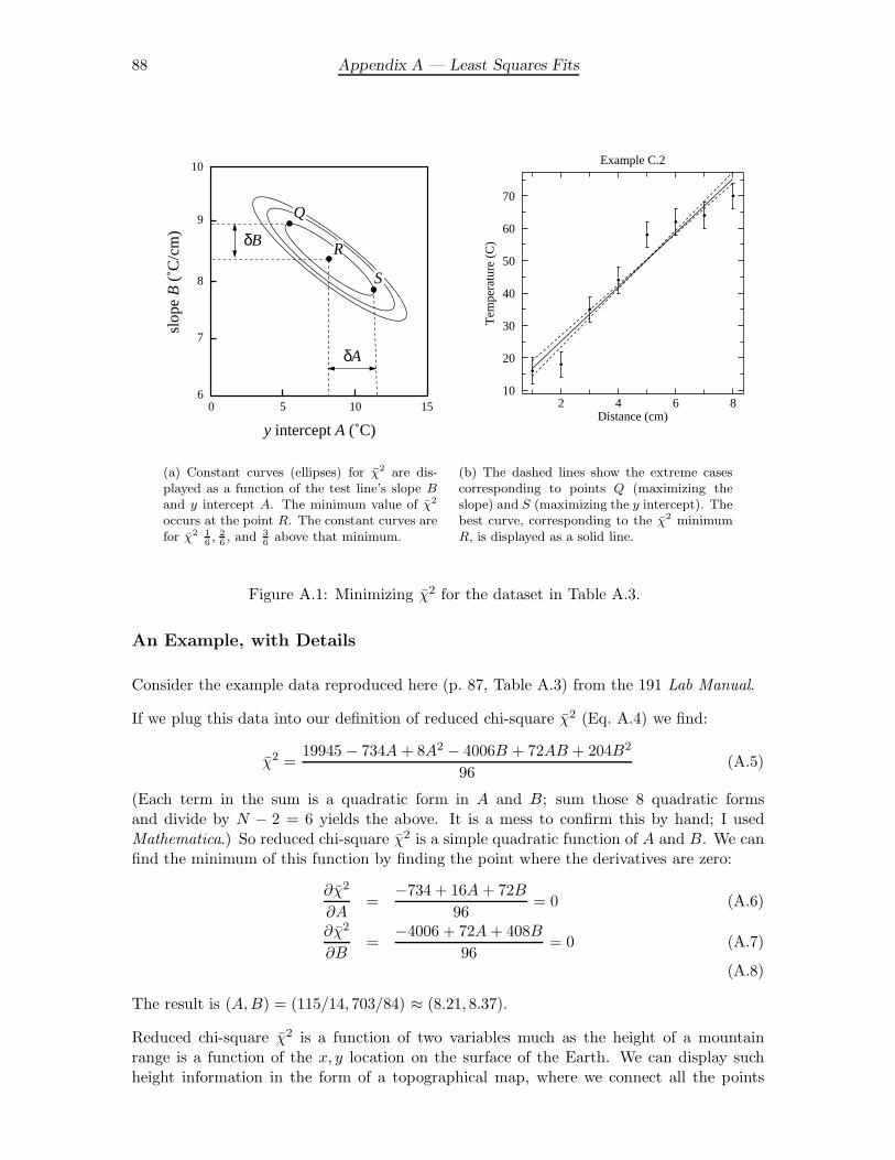
88 Appendix A — Least Squares Fits
6
7
8
9
10
0 5 10 15
y intercept A (˚C)
slop
e B (
˚C/c
m)
δA
δB
Q
R
S
(a) Constant curves (ellipses) for χ2 are dis-played as a function of the test line’s slope B
and y intercept A. The minimum value of χ2
occurs at the point R. The constant curves arefor χ2 1
6, 2
6, and 3
6above that minimum.
2 4 6 8
70
60
50
40
30
20
10
Example C.2
Distance (cm)
Tem
pera
ture
(C
)(b) The dashed lines show the extreme casescorresponding to points Q (maximizing theslope) and S (maximizing the y intercept). Thebest curve, corresponding to the χ2 minimumR, is displayed as a solid line.
Figure A.1: Minimizing χ2 for the dataset in Table A.3.
An Example, with Details
Consider the example data reproduced here (p. 87, Table A.3) from the 191 Lab Manual.
If we plug this data into our definition of reduced chi-square χ2 (Eq. A.4) we find:
χ2 =19945 − 734A + 8A2 − 4006B + 72AB + 204B2
96(A.5)
(Each term in the sum is a quadratic form in A and B; sum those 8 quadratic formsand divide by N − 2 = 6 yields the above. It is a mess to confirm this by hand; I usedMathematica.) So reduced chi-square χ2 is a simple quadratic function of A and B. We canfind the minimum of this function by finding the point where the derivatives are zero:
∂χ2
∂A=
−734 + 16A + 72B
96= 0 (A.6)
∂χ2
∂B=
−4006 + 72A + 408B
96= 0 (A.7)
(A.8)
The result is (A,B) = (115/14, 703/84) ≈ (8.21, 8.37).
Reduced chi-square χ2 is a function of two variables much as the height of a mountainrange is a function of the x, y location on the surface of the Earth. We can display suchheight information in the form of a topographical map, where we connect all the points

Appendix A — Least Squares Fits 89
that are at the same altitude. In a similar way we can display the function χ2(A,B), byshowing the collection of points where χ2(A,B) equals some constant. (See Figure A.1(a).)Since χ2(A,B) is a simple quadratic form the resulting constant curves are ellipses, and the‘topography’ is quite simple with a single valley, oriented diagonally, with minimum at thepoint R. The uncertainly in the best fit parameters is determined by topography aroundthat minimum: how much can a parameter vary before the resulting line is a detectablyworst fit. The definition of ‘detectably worst’ is where the chi-square sum has increasedby one unit above the minimum. The extreme points Q and S are displayed in the abovefigure along with the corresponding lines.
In more complicated situations, the chi-square topography can become much more complex,with several local valleys (which makes finding the global minimum more difficult). In thesimplest cases (like that discussed above) the derivatives of chi-square are easily solvedlinear equations with a unique solution (hence just one valley). These cases are known aslinear least squares.
You may be surprised at the relatively small range of variation implied by the parametererrors and displayed in Fig. A.1(b). Recall that the parameters are estimates of averagebehavior revealed by the assumed unbiased deviations. So much as the standard deviationof the mean is smaller than the standard deviation (and in fact can get arbitrarily smallwith sufficiently large data sets), so too the parameter uncertainties become increasinglysmall with large data sets. As a result the systematic errors must dominate the randomerrors for sufficiently large data sets, in which case the computer reported errors are notrelevant.
Introduction to WAPP+
There are many computer programs that can do least-squares fits. In this laboratory wewill use the web-based program WAPP+ located at:http://www.physics.csbsju.edu/stats/WAPP2.html.I suggest you add it to your favorites2.
On the opening page of WAPP+ you must report the format of your data, particularlyfor the uncertainty in your data:
• No y error
Select this if your y data has no error (unlikely) or if you have no estimate for thaterror (rare) or if you have been told that the error is “negligible”.
• Enter a formula for y error
It is not uncommon to have a simple formula for your errors. In the simplest possiblecase your error may be a constant. Often you will know the error as a fraction(or percentage) of the y value. Very occasionally you may know a fairly complexformula for the error. (For example, in Physics 200, one error is calculated from:(y^2+1)*pi/90.) If you have such a formula, you may supply it to the program to
2a Google for “wapp+” will provide a link or you can hit the statistics link on the Physics homepage:www.physics.csbsju.edu

90 Appendix A — Least Squares Fits
calculate the errors for you. Alternatively you could use a spreadsheet or calculatorto calculate those errors and just enter them along with your data.
• Enter y error for each data point
Sometimes errors are estimated as part of the experiment by repeating the experimentand looking for deviations. In this case the errors are likely to be different for eachdata point and there will be no formula to apply.
Exactly analogous boxes must be checked to indicate the nature of x errors.
There are two ways of entering your data into the computer: copy & paste from a spread-sheet (the usual approach because using a spreadsheet is often required for other parts ofthe experiment) or entering each number into its own box on the web page. I would alwaysopt for the former (“bulk” or copy & paste), but if you really want to you may use the
latter (“pointwise data entry”). The following paragraphs assume Do Bulk was selected.)
On the second page of WAPP+ you must enter your data+errors and select which functionapplies to your data.
If you selected to enter errors with a formula, boxes to enter those formulae appear on thetop of the page. For example, in Lab 1 you are told that the error in x is 0.5% and theerror in y is given by the formula: δθ(1 + y2), where δθ might be estimated as .035 rad, soyou would enter:
y-error= .035*(1+y^2)
x-error= .005*x
If you selected individualized errors, you will enter those errors along with the correspondingdata. Two options are provided: you may do a “Block Copy & Paste” of all the data anderrors (and perhaps columns to be ignored) or you may use the “Column Copy & Paste”area to separately paste each column of the requested data. (In either case the columnheadings should be a reminder of what you reported you were going to provide. E.g., if youare presented with a “X Errors” option or a “XE” column, you told the program on theprevious page that you would supply individualized x-errors.)
I usually use the “Block Copy & Paste” pseudo spreadsheet. There WAPP+ presents a bigarea to enter numbers with multiple-choice column headers:
column1 column2 column3 column4 column5 column6
None None None None None None
Often I arrange my spreadsheet so that x, δx, y, δy are in adjacent columns in which case Iwould select:
column1 column2 column3 column4 column5 column6
X X Errors Y Y Errors None None
Sometimes you will have a column of irrelevant data between required data: no problem,just tell WAPP+ to Ignore the irrelevant column.
Note: The apparent grid of cells and columns in the “Block Copy & Paste” web-form,

Appendix A — Least Squares Fits 91
in fact, have no meaning: it’s just an image to remind you that this area will be filled bypasting data from a spreadsheet. The pasted data does not have to line up in columns(the white space between the numbers is what denotes column boundaries). You do need toassure that the number of numbers in each row matches the number of columns not selectedas None. In addition, pasted data must be numbers not text (for example: column labels).Finally an extra Enter at the end of the last data item may avoid IE transfer problems.
If you decide to use “Column Copy & Paste” simply select the appropriate single columnof values in your spreadsheet and paste it into the appropriate WAPP+ column. Typicallyseveral separate copy&paste moves will be needed to fill all the columns. Of course, eachcolumn must contain the data in the same order. (Note: you can also enter some data via“Block Copy & Paste” with the remaining data supplied via “Column Copy & Paste”.)
Near the bottom of this page you select which function should fit the data.
When you Submit Data , the third page of WAPP+ arrives: this is your “fit report”.Almost always you will want to select the top region of this page, print it out, and tape itinto your notebook. Here is page generated by the data from Table A.3.
An analysis of data submitted by computer: linphys1.physics.csbsju.edu on 1-APR-2010 at13:35 indicates that a function of the form:—Linear— y = A + Bxcan fit the 8 data points with a reduced chi-squared of 1.7
FIT
PARAMETER VALUE ERROR
A = 8.214 3.1
B = 8.369 0.62
NO x-errors
ACTUAL ERROR IN CALCULATED DEVIATION
POINT X Y Y Y FROM FIT
1 1.00 16.0 +- 4.0 16.6 -0.583
2 2.00 18.0 +- 4.0 25.0 -6.95
3 3.00 35.0 +- 4.0 33.3 1.68
4 4.00 44.0 +- 4.0 41.7 2.31
5 5.00 58.0 +- 4.0 50.1 7.94
6 6.00 62.0 +- 4.0 58.4 3.57
7 7.00 64.0 +- 4.0 66.8 -2.80
8 8.00 70.0 +- 4.0 75.2 -5.17
Data Reference: 626A
It is perhaps worth reminding you that computers are usually ignorant of sigfigs and units:I would report these results as: A = 8 ± 3 C and B = 8.4 ± .6 C/cm. AlternativelyA = 8.2± 3.1 C and B = 8.37± .62 C/cm is also OK; other possibilities are incorrect andwill result in lost points.
The Data Reference: 626A at the bottom is useful and should be retained. If some problem(e.g., a computer crash) should occur, it is likely that this reference will allow you to get a

92 Appendix A — Least Squares Fits
copy of your data from the web.
The bottom part of this page allows you to make various types of plots of your results.If you click on Make Plot a fourth page pops up with links to the actual plots. Mostcommonly you will click on the PDF File, Adobe Acrobat will launch and your plot will bedisplayed, and if desired printed.
How to enter formulas: The usual syntax applies: + − * / for add, subtract, multiply,and divide respectively; ^ or ** for powers. Please note:
A/B ∗ C =AC
B(A.9)
A/(B ∗ C) =A
BC(A.10)
Mathematical functions for formulas:
ABS ACOS ASIN ATANCOS COSH ERF ERFCEXP INT LOG LOG10NINT RAN SCALE SIGNSIN SINH SQRT TANTANH GAMMA K NORMINORM PI

Appendix B — Meter UncertaintySpecifications
93
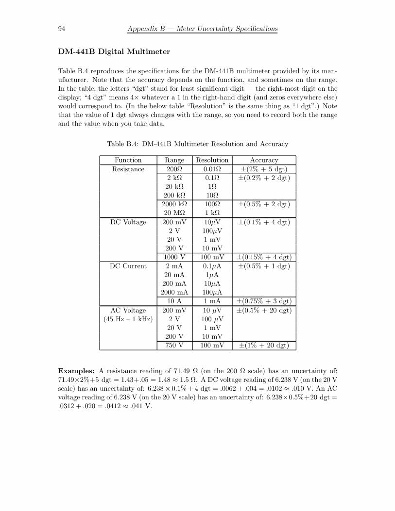
94 Appendix B — Meter Uncertainty Specifications
DM-441B Digital Multimeter
Table B.4 reproduces the specifications for the DM-441B multimeter provided by its man-ufacturer. Note that the accuracy depends on the function, and sometimes on the range.In the table, the letters “dgt” stand for least significant digit — the right-most digit on thedisplay; “4 dgt” means 4× whatever a 1 in the right-hand digit (and zeros everywhere else)would correspond to. (In the below table “Resolution” is the same thing as “1 dgt”.) Notethat the value of 1 dgt always changes with the range, so you need to record both the rangeand the value when you take data.
Table B.4: DM-441B Multimeter Resolution and Accuracy
Function Range Resolution Accuracy
Resistance 200Ω 0.01Ω ±(2% + 5 dgt)2 kΩ 0.1Ω ±(0.2% + 2 dgt)20 kΩ 1Ω200 kΩ 10Ω2000 kΩ 100Ω ±(0.5% + 2 dgt)20 MΩ 1 kΩ
DC Voltage 200 mV 10µV ±(0.1% + 4 dgt)2 V 100µV20 V 1 mV200 V 10 mV1000 V 100 mV ±(0.15% + 4 dgt)
DC Current 2 mA 0.1µA ±(0.5% + 1 dgt)20 mA 1µA200 mA 10µA2000 mA 100µA
10 A 1 mA ±(0.75% + 3 dgt)
AC Voltage 200 mV 10 µV ±(0.5% + 20 dgt)(45 Hz – 1 kHz) 2 V 100 µV
20 V 1 mV200 V 10 mV750 V 100 mV ±(1% + 20 dgt)
Examples: A resistance reading of 71.49 Ω (on the 200 Ω scale) has an uncertainty of:71.49×2%+5 dgt = 1.43+.05 = 1.48 ≈ 1.5 Ω. A DC voltage reading of 6.238 V (on the 20 Vscale) has an uncertainty of: 6.238× 0.1% + 4 dgt = .0062 + .004 = .0102 ≈ .010 V. An ACvoltage reading of 6.238 V (on the 20 V scale) has an uncertainty of: 6.238×0.5%+20 dgt =.0312 + .020 = .0412 ≈ .041 V.

Appendix B — Meter Uncertainty Specifications 95
Wavetek Model 19 Function Generator
Display Accuracy
Frequency: ± 1 digit on 2 kHz to 2 MHz ranges;< or = 1.5% of full scale on 2 Hz to 200 Hz ranges
Amplitude: Typically 5% of range at 1 kHz.
DC offset: Typically 2% of reading.
Resolution: 0.05% maximum on all ranges
Tektronix TDS 200-Series Digital Oscilloscope
Vertical Measurement Accuracy in Average Acquisition Mode (> 16 waveforms)
DC measurement with ± (4% × reading + 0.1 div + 1 mV)vertical position at zero
DC measurement with ± [3% × (reading + vertical position) + 1% of verticalvertical position not at zero position + 0.2 div]. Add 2 mV for settings from
2 mV/div to 200 mV/div. Add 50 mV for settingsfrom > 200 mV/div to 5 V/div.
Delta volts measurement ± (3% × reading + 0.05 div)
Horizontal Measurement Accuracy
Delta time measurement ± (1 sample interval* + .01% × reading + 0.6 ns)Single-shot sample mode
Delta time measurement ± (1 sample interval* + .01% × reading + 0.4 ns)> 16 averages
*Sample interval = (s/div)/250

96 Appendix B — Meter Uncertainty Specifications

Appendix C — UncertaintyFormulae
97
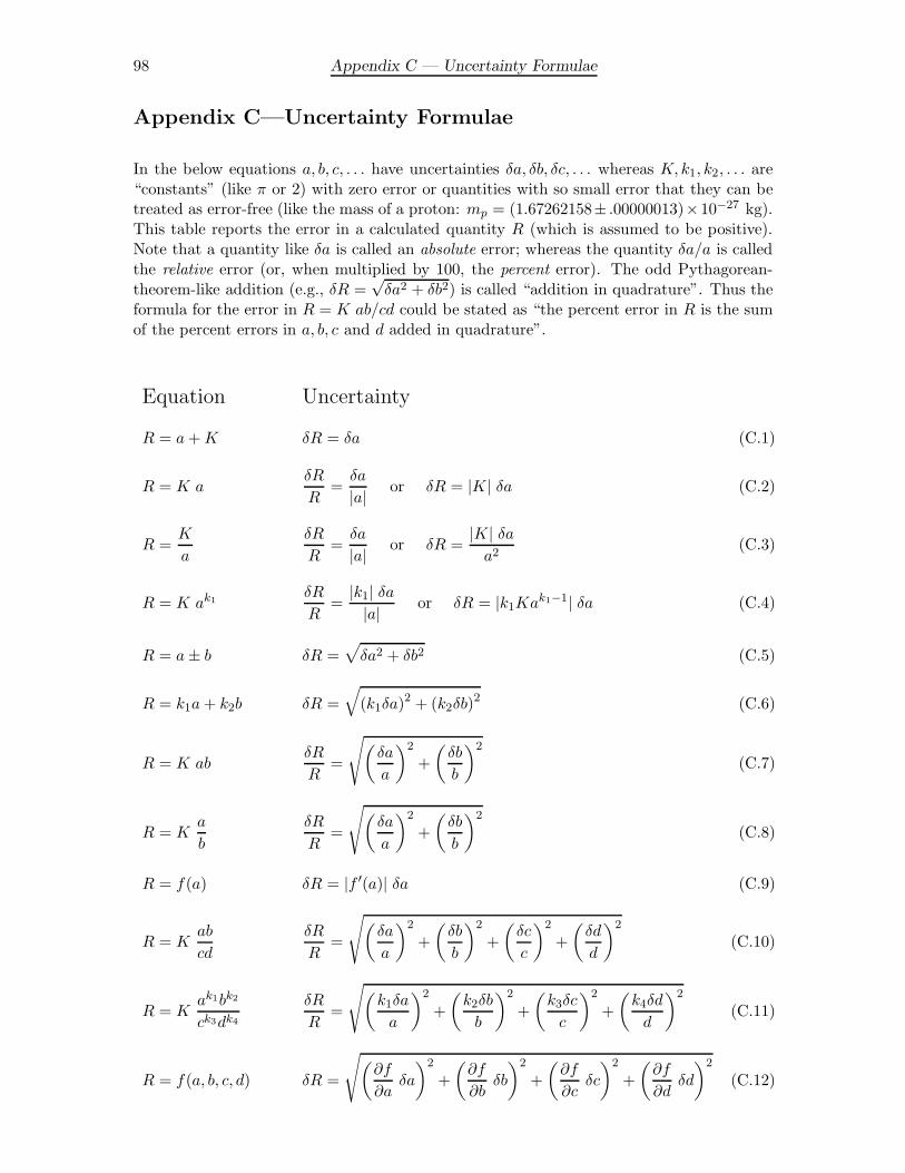
98 Appendix C — Uncertainty Formulae
Appendix C—Uncertainty Formulae
In the below equations a, b, c, . . . have uncertainties δa, δb, δc, . . . whereas K,k1, k2, . . . are“constants” (like π or 2) with zero error or quantities with so small error that they can betreated as error-free (like the mass of a proton: mp = (1.67262158± .00000013)×10−27 kg).This table reports the error in a calculated quantity R (which is assumed to be positive).Note that a quantity like δa is called an absolute error; whereas the quantity δa/a is calledthe relative error (or, when multiplied by 100, the percent error). The odd Pythagorean-theorem-like addition (e.g., δR =
√δa2 + δb2) is called “addition in quadrature”. Thus the
formula for the error in R = K ab/cd could be stated as “the percent error in R is the sumof the percent errors in a, b, c and d added in quadrature”.
Equation Uncertainty
R = a + K δR = δa (C.1)
R = K aδR
R=
δa
|a| or δR = |K| δa (C.2)
R =K
a
δR
R=
δa
|a| or δR =|K| δa
a2(C.3)
R = K ak1δR
R=
|k1| δa
|a| or δR = |k1Kak1−1| δa (C.4)
R = a ± b δR =√
δa2 + δb2 (C.5)
R = k1a + k2b δR =
√
(k1δa)2 + (k2δb)2 (C.6)
R = K abδR
R=
√
(
δa
a
)2
+
(
δb
b
)2
(C.7)
R = Ka
b
δR
R=
√
(
δa
a
)2
+
(
δb
b
)2
(C.8)
R = f(a) δR = |f ′(a)| δa (C.9)
R = Kab
cd
δR
R=
√
(
δa
a
)2
+
(
δb
b
)2
+
(
δc
c
)2
+
(
δd
d
)2
(C.10)
R = Kak1bk2
ck3dk4
δR
R=
√
(
k1δa
a
)2
+
(
k2δb
b
)2
+
(
k3δc
c
)2
+
(
k4δd
d
)2
(C.11)
R = f(a, b, c, d) δR =
√
(
∂f
∂aδa
)2
+
(
∂f
∂bδb
)2
+
(
∂f
∂cδc
)2
+
(
∂f
∂dδd
)2
(C.12)