International Journal of Mass Spectrometry and Ion Processes, 13 (1986) 109-125 Elsevier Science Publishers B.V., Amsterdam - Printed in The Netherlands

109

PEAK SHAPE DETERMINATION IN LASER MICROPROBE MASS ANALYSIS

A. VERTES, P. JUHASZ and L. MATUS

Central Research Institute for Physics, Hungarian Academ_v of Sciences,

P.O. Box 49, H-l 525 Budapest (Hungaty)

(Received 2 May. 1986)

ABSTRACT

Potential distribution and ion trajectory calculations involving time development of the ion motion in laser microprobe mass spectrometers have been performed. Potential distribu- tion calculations were based on the Fourier transformation technique since this offers improved effectiveness. The time-dependent ion trajectories that were calculated showed different flight times for ions with different initial conditions.

Transmission properties of the angle focusing “einzel” lens are discussed with special emphasis on lens potential and ion formation position dependence. Qualitative agreement with experimental findings is demonstrated.

It was shown that, if the geometrical parameters of the instrument are optimized, an arrangement promising similar performance to that of LAMMA 500 can be obtained but with more compact design.

Peak shape calculations were carried out for different initial kinetic energy and departing angle distributions. Peak broadening, shift, and asymmetry could be explained in terms of the width of ion energy distribution. However, no dramatic broadening was observed according to the second-order energy focusing property of the ion reflector.

INTRODUCTION

Laser ionization mass spectrometry has gained considerable importance since the end of the seventies and the beginning of the eighties when commercially available instruments (e.g. LAMMA 500, Leybold-Heraeus, Cologne, F.R.G.) became widely available. Their popularity is supported by the high throughput performance, high absolute sensitivity (1O-‘x to 10e20 g) and local analysis capability (down to 1-2 pm lateral resolution).

It quickly became apparent, however, that no simple interpretation of the spectra was possible. The energy spread of ions in laser-produced plasmas at power densities of the order of 10” W cm- * typically exceeds several hundred eV [l], whereas local thermal equilibrium calculations predicted

0168-1176/86/$03.50 C, 1986 Elsevier Science Publishers B.V.

110

0.4-1.1 eV [2]. The difficulties related to spectrum interpretation can be divided into two groups. Physical processes during the interaction of laser light with the solid target and the microplasma on the one hand and transmission properties of the analysis and detection system on the other are the main factors influencing the type and quantity of the ions detected.

Several attempts have been made to try to understand the basic processes as well as the instrumental effects in laser ionization ion sources and mass spectrometers. Progress in this field would be beneficial in order to achieve firmer ground for qualitative and quantitative evaluation of mass spectra.

The basic processes occurring in laser-induced plasmas have been dis- cussed from the point of view of the similar conditions obtaining in the thermonuclear fusion [3] and heavy-ion sources [4]. Mauney and Adams [5] developed a method of measuring the initial kinetic energy distribution of ions in laser-induced plasmas. Their experiment was based on the energy cut-off property of the ion reflector in the laser microprobe mass analyser (LAMMA) instrument. Michiels et al. [6] employed the method to measure ion energy distributions in microplasmas on TiO, targets. Another approach to the problem of LAMMA spectra is to focus on the transmission proper- ties of the instrument itself and Michiels et al. [7] discovered ion discrimina- tion effects in the LAMMA instrument which were mainly due to aberra- tions of the “einzel” lens in the ion optical system.

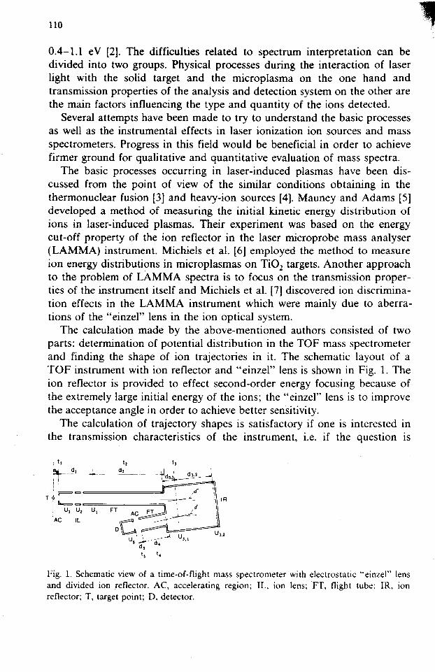
The calculation made by the above-mentioned authors consisted of two parts: determination of potential distribution in the TOF mass spectrometer and finding the shape of ion trajectories in it. The schematic layout of a TOF instrument with ion reflector and “einzel” lens is shown in Fig. 1. The ion reflector is provided to effect second-order energy focusing because of the extremely large initial energy of the ions; the “einzel” lens is to improve the acceptance angle in order to achieve better sensitivity.

The calculation of trajectory shapes is satisfactory if one is interested the transmission characteristics of the instrument, i.e. if the question

in is

Fig. 1. Schematic view of a time-of-flight mass spectrometer with electrostatic “einzel” lens and divided ion reflector. AC, accelerating region; IL, ion lens; .FT, flight tube; IR, ion reflector; T, target point; D, detector.

111

whether or not a given ion with fixed initial energy and departing angle will travel through the spectrometer and hit the detector. It is equally important, however, to know the flight time related to that particular trajectory. This will, of course, vary from trajectory to trajectory and hence produce a flight time distribution for each type of ion. Consequently, the spectrum consists of peaks of different shape instead of sharp lines.

Our goal is to investigate the role of different factors influencing peak shapes with special emphasis on instrumental effects. To achieve this, we calculate the potential distribution in different parts of the instrument. The next step is to trace trajectory shapes and determine corresponding flight times. At the same time, this procedure gives us the opportunity to explore the optimal electrode geometry for a laser ionization mass spectrometer or even to propose a new version with divided ion reflector promising more compactness and the same performance.

METHODS OF CALCULATION

Ion trajectories are easy to follow in field-free regions or in homogeneous electrostatic fields using well-known classical mechanical formulae. We have to apply them to ion drift in the flight-tube of the time-of-flight (TOF) mass spectrometer and to the ion reflector where, in a homogeneous field, second-order energy focusing takes place IS].

More computational work is needed in the case of inhomogeneous regions where, in general, the potential field cannot be given in closed analytical form but as a numerical solution of the Laplace equation. It forms a Dirichlet problem together with the boundary condition. lon trajectories are then solutions of equations of motion containing field-gradients which were determined previously. This kind of calculation has been carried out for the “einzel’‘-type ion lens.

Our task is then to determine the electrostatic potential distribution within the ion lens and then to integrate the equations of motionnumeri- tally. In the remaining part of the TOF mass spectrometer, analytical formulae may be utilized.

For determining potential maps of electrostatic lenses, numerous well- studied methods are at hand [9.10]: here. we mention the most widespread. The most exact and general method of calculating a potential distribution with arbitrary boundary condition is the charge-density method [ll]. which does not contain any additional assumption concerning the boundary condi- tion. However, it is often useful to make reasonable assumptions to simplify numerical solution (e.g. to consider the boundary continuous, which is not the case with the “einzel” lens, i.e. separated rings).

The most widespread technique is the numerical solution of Laplace’s

112

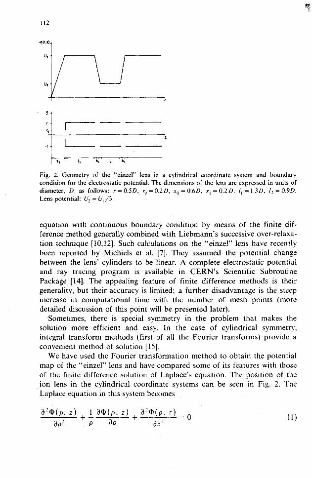
Fig. 2. Geometry of the “einzel” lens in a cylindrical coordinate system and boundary condition for the electrostatic potential. The dimensions of the lens are expressed in units of diameter, D, as follows: r=0.5D,.ro=0.2D, s,=OhD, s,=O.ZD, 1,=1.30, 1?=0.9D. Lens potential: Uz = U,/3.

equation with continuous boundary condition by means of the finite dif- ference method generally combined with Liebmann’s successive over-relaxa- tion technique [10,12]. Such calculations on the “einzel” lens have recently been reported by Michiels et al. [7]. They assumed the potential change between the lens’ cylinders to be linear. A complete electrostatic potential and ray tracing program is available in CERN’s Scientific Subroutine Package [14]. The appealing feature of finite difference methods is their generality, but their accuracy is limited; a further disadvantage is the steep increase in computational time with the number of mesh points (more detailed discussion of this point will be presented later).

-Sometimes, there is special symmetry in the problem that makes the solution more efficient and easy. In the case of cylindrical symmetry, integral transform methods (first of all the Fourier transforms) provide a convenient method of solution [15].

We have used the Fourier transformation method to obtain the potential map of the “einzel” lens and have compared some of its features with those of the finite difference solution of Laplace’s equation. The position of the ion lens in the cylindrical coordinate systems can be seen in Fig. 2. The Laplace equation in this system becomes

113

with the boundary conditions

@(T, z) = f(z)

@(p, 0) = 0

(2a)

(2b) where r is the lens’ radius and potential changes between the cylinders are considered linear.

Taking the Fourier transform with respect to z, we get

a2F#] + 1 %[@I ap2 P aP -

cd2 = 0 (3)

where F,[ a’] is the complex Fourier transform of potential distribution

F_[Q] =/= e-‘“‘Q,(p, z) dz (4) --cc

Equation (3) has a regular solution: the modified Bessel function of zeroth order, I,, with which the complete solution of Eq. (4) with boundary conditions (2a) and (2b) can be written as

(5)

where F_[ f] is the Fourier transform of boundary condition (2a). The Fourier transformation method has some advantages over the finite

difference method, mainly concerning accuracy and computational time. Equation (5) is an analytical solution of the Dirichlet problem in the radial variable (not approximate) and it can also be made arbitrarily accurate axially by increasing the number of axial mesh points. The total number of mesh points in the finite difference method is limited; for example, it should not exceed 2900 in the CERN program [14], whereas the Fourier transfor- mation method has less strong limitations in this respect. We used an 80 x 512 mesh, i.e. 40960 mesh points.

Let us consider a mesh that covers the lens containing M X N points. In the case of the finite difference method (with successive over-relaxation), the computational time varies approximately as 6( A4 x N )’ [lb]; for the Fourier transformation method, this dependence is 2NM log, M, if A4 is an integer power of 2 [17]. From these features, the Fourier transformation method seems to be more convenient, quicker, and more accurate in cylindrically symmetric problems than are finite difference techniques.

Most calculations and discussions dealing with particle trajectories in electrostatic lenses are based on the numerical integration of the so-called ray equation

d2p 1 + (dp/dz)2 dp @D(p, -_) -= -- d;’ WP, 4 d,_ a: I

(6)

&.$.“. J,

114

where space-charge effects are neglected [18]. This equation can be sim- plified if one utilizes the paraxial condition, i.e. d@/dp = 0, thus, the first term of the right-hand side of Eq. (6) vanishes and we get the well-known paraxial equation, which is often accurate enough for planning and optimiz- ing electrostatic lenses [9,13].

Sometimes we need not only the shapes of trajectories but also their time evolution. This is the case, for example, if we wish to predict peak shapes from accurately calculated flight times. For this purpose, we apply the classical equations of motion in Newtonian form

d%(t) e d@‘(P, 4 --_=-- dt* m ap

Pa)

d*z( t ) e wp, Z) p=-- dt* m aZ

with the initial conditions

p(0) = z(0) = 0

dP(O) dt=l) 0.P

Wo) dt=” 0.:

Pb)

(84

Gw

(84 To avoid superfluous calculations such as estimation of first time deriva-

tives and relatively inaccurate extrapolations (these are consequences of the implicit character of Newtonian equations), we applied the Cowell-Numerov method which is particularly suitable for integrating differential equations of the form 1191

_Y”= f(& y) (9)

For Eq. (9), the scheme _

h2 Y ?l+1 = 2Yn -Yn-l+ ,,un+, + lO_L +fn-d

yields the solution with local truncation error h6Yv’( n)/240, where h is the integration stepsize and yvl( n) the value of the sixth derivative at the n th point (in time).

Care must be taken with the implicit nature of Eq. (10): it contains the (n + l)th function value, f,, 1, which means that, in Eq. (ll), there are two unknown quantities. We have thus had to use some reasonable extrapolation

to fn+1 which, of course, may significantly increase the above-mentioned truncation error. It is easy, however, to prove that, even with linear extrapo- lation, h can always be chosen in such a way that if potential gradients are

115

everywhere bounded, the error of the potential map (between the mesh points) will dominate the overall error of the trajectory tracing procedure.

This integration technique has been used to determine ion trajectory shapes and flight times in the ion lens and its results determined the initial conditions for ion motion in the remaining part of the TOF apparatus.

The TOF instrument with ion reflector is illustrated in Fig. 1. Flight times, as mentioned earlier, can be calculated by classical mechanical formulae. The initial conditions are given by the initial kinetic energy exit position and angle at the end of the ion lens. The total flight time may be written as

t = t, + t, + t, + t, + t,

where t, is the flight time in the ion lens. The remaining terms are

(11)

t, = 2m4,1 2eUl ‘I2

e(U,., - UI) [i 1 sin a - 2eUl

m i m sin’ (Y’ - 2e( U,.,

+ 2m4.z 2eZJ, l/2

44.2 - u,.J [ -sin2 a’ - 2e(U3,, - U,)/m

IyI I

l/2

Ul J/m i I

(12b)

1 coseco,[d, - [%)li2 sin G(sin 8 - cos cd)t3] (12~)

cos (Yg - 2eU, -cos2 a0 - 2e( U, - U,)/m

m

(124 where the symbols are the same as for Fig. 1; y0 gives the initial distance from the axis of the flight tube, (Y,, is the initial angle of the drift, and (Y’ = 90” - s + CYc).

We have dealt with single and double stage ion reflectors. The latter offers a more compact experimental set-up, with the same efficiency in energy focusing, than a homogeneous reflector [20].

For actual peak shape calculations, we chose a reference trajectory characterized by zero initial kinetic energy and coincidence with the axis of the flight tube. We calculated the time deviation between particles on ion trajectories with systematically varied initial conditions and particles on the reference trajectory.

As an ensemble of systematically varied initial conditions, one can accept an initial angular and kinetic energy distribution of laser-induced ions for

I 116

modelling the situation immediately after ionization. This initial distribution is modified by the ion lens. The new angular and kinetic energy distribution (after passing the ion lens) can be determined by Cowell-Numerov integra- tion of Eqs. (7a) and (7b). Only those trajectories have to be followed for which their respective deflection from the reference trajectory does not exceed the angle acceptance of the remaining part of the instrument, i.e. those that can be seen from the active surface of the detector. Flight times are then calculated using Eqs. (12a)-(12d), giving the total time associated with a single trajectory.

Calculations were performed on an IBM PC microcomputer. The numeri- cal methods described above do not require a mini or mainframe, unlike finite difference methods; they can readily be implemented by personal computers. A typical run time for potential map determination on a 40960 point mesh takes about 4 min. A 500-step integration of equations of motion lasts for about 6 s trajectory-‘. (The source code is available upon request.)

RESULTS AND DISCUSSION

The accelerating region and the ion lens were first investigated separately. Similar lenses are well described in the literature from the point of view of imaging and focusing behaviour [13], but no flight time characteristics are available. Properties especially interesting are flight times belonging to different trajectories, residual angle divergence after the lens, and transmis- sion as a function of lens potential as well as position of ion formation.

The limiting aperture cuts out rays with large initial energy and departing angle in accordance with the inequality

a2 xc

sin’ cyO.- a sin(2cw,) (13)

where x = Ekin/Ul and a = r,/2s,. Trajectories satisfying this condition were traced further.

The relative time deviation as a function of initial kinetic energy (in units of accelerating voltage) for different departing angles is shown in Fig. 3. Particles travelling along the axis showed a pronounced decrease in flight time with increasing energy. Tilting the vector of initial velocity compensates this effect because of the increased path and consequently flight time, in accordance with the curved trajectory in inhomogeneous field regions. At 60” departing angle (curve d) considerable energy focusing of the “einzel” lens can be observed. This unexpected feature may have further potential for specific applications, where a combination of angle and energy focusing in

117

Fig. 3. Relative deviation in flight times and residual divergence of trajectories for the “einzel” lens at different initial ion energies. Curves a, b, c, d, and e correspond to 0, 20, 40, 60, and 80’ departing angles, respectively.

one step would be beneficial. The obvious shortcoming of this solution would be the much poorer transmission than otherwise provided by the lens. The curves in Fig. 3 corresponding to angles larger than 20” stop at energies leading to trajectories which hit the wall inside the lens.

The other set of curves in Fig. 3 describes the dependence of residual deflection beyond the lens on initial kinetic energy at different departing angles. It is demonstrated that the lens operates quite well for rays with departing angles below 20”.

We also varied the lens potential to see what effect this would have on its transmission. We took 961 trajectories of uniform energy and isotropic departing angle distributions for ions at the target point. The energy was increased from 0 to 6.6% of the accelerating voltage, while the departing angle was varied from 0 to 90” in 31 steps each. A particle has been claimed to be transmitted if its residual deflection did not exceed 1 or 0.1” depending on the rigour of the definition. Both curves show a definite maximum, as can be seen in Fig. 4. Optimal lens voltages for 1 and 0.1” residual divergence are U/U, = 0.36 and U/U, = 0.31, respectively.

It is interesting to compare these curves with the measured transmission characteristics of the LAMMA 500 instrument. Investigation of the ion optical properties of the LAMMA 500 with continuous ion source provided ion current data as a function of lens potential [5]. Since no field penetration from the lens to the accelerating region occurs, the current values are proportional to the transmission of the lens itself. The experimental points scaled in arbitrary units are also displayed in Fig. 4. Its shape is fairly

118

Fig. 4. Transmission of “einzel” lens as a function of reduced lens potential for two different values of the allowed residual angle divergence (1 and 0.1’). The experimental curve (exp.) is from ref. 5 where the ion current in LAMMA 500 was measured as a function of lens potential. (The data of ref. 5 are displayed here in arbitrary current units.)

similar to the curve corresponding to 0.1” residual divergence. The positions of their maxima are almost identical. There are, however, marked differences too. The experimental curve starts from almost zero and exhibits steeper increase and faster decay than the calculated curve.

In this way, we arrive at the conclusion that the angle acceptance of the instrument after the lens is close to O.l”, and besides the lens there are other factors, e.g. the energy cut-off of the ion reflector, governing the overall transmission of the instrument. Furthermore, there is another possible origin of the differences, viz. the fact that the experimental points are results obtained with a thermal ion source supplying much less energetic ions than the ones we used in our model for laser excitation.

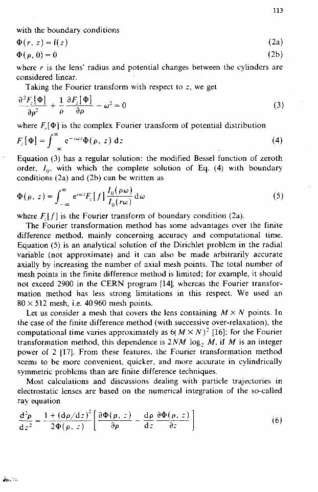
A similar set of calculations was carried out to explore the effect of the axial position of ion formation -on the transmission. We fixed the lens potential at U/U, = 0.33 and varied the origin of ion trajectories in the range of 0.0 < z,/s, c 0.35. As expected, monotonic decrease of transmis- sion was observed in the case of lo residual angle divergence. Surprisingly enough, this was not the case for 0.1”. The maximum transmission belongs to trajectories starting from z,/s, = 0.05 in front of the target point. This astonishing effect is probably due to unbalanced chromatic aberration, i.e. energy dispersion of the electrostatic lens. Mauney and Adams measured the ion current as a function of filament position in their continuous thermal ionization ion source and found monotonic decay (51, which also supports our idea since the ions in this experiment were practically monoenergetic. Calculated and measured curves are given in Fig. 5.

119

Fig. 5. Axial position of ion forination also has a considerable influence on lens transmission. The axial position from the target point is expressed in units of the length of accelerating region, s,,. The origin and units for the experimental curve are the same as in Fig. 4.

In order to determine the optimal geometry for energy focusing, one has to investigate the flight time formulae Eqs. (11) and (12). The relative flight time deviation for the whole instrument has been calculated as a function of the initial energy of the ions. We applied a global condition for resolving peaks M and M + 1

maxIT(M, E,;,)/T(M, 0) - 11 +C T(M+ l,O)/T(M, 0) - 1 (14)

whenever 0 < Ekin < E,,, where E,,, is the energy acceptance. of the spec- trometer. This is a more strict condition for energy focusing than the usual second-order local criterion based on derivatives of Eqs. (11) and (12) with respect t0 Ekin.

Optimal geometry was sought with a computer code for solving multi-di- mensional non-linear extremum problems. To speed up computations we replaced t, with its simplified value neglecting the time shift due to the lens potential. This is, of course, an approximation forced by practical reasons and can be justified only by experimental facts. The set of independent variables, sO, d, + d2 + d,; d,.,, d,.2; 8; U3,1/U3,2, forms a six-dimensional parameter space for a divided, and a five-dimensional sub-space for a single ion reflector, obeying L&/d,., = U3.,/d,., in the latter case. Our domain of interest in the parameter space has been greatly limited by technological and practical constraints, such as compactness, electrical insulation of different parts, etc.

Inequality (14) served as the criterion for finding optimal parameters. In the case of M = 250 and E,,, = 200 eV, the right-hand side = 0.002 whereas the left-hand side < 0.0003 if we choose sg = 5 mm. d, + d, + d, = 1390

120

mm, d3 1 + 4.2 = 430 mm, d, = 10 mm, S = 4”. Lfl = - 3000 V, rj; 1 + Q2 = 500 q, U, = - 5000 V. This single-stage instrument reminded us very much of the commercially available LAMMA 500, having s0 = 5.75 mm, d, + d, + d, = 1469.25 mm, d, 1 + d,., = 407.6 mm, d, = 10 mm and 8 = 3”.

However, if a double-stage ion reflector was introduced, we could achieve a more compact design with similar performance. The principle of the double-stage ion reflector is to instantly decelerate the ions in a high field gradient first stage and then turn these slow particles back in a low field gradient second stage in order to perform energy focusing. Because the particle’s orbit can be more depressed than in the single-stage reflector, the reflector itself can be much more compact. In fact, optimizing with the same procedure, we obtained slightly better resolving power than with a single- stage instrument using the geometrical parameters s0 = 5 mm, d, + d, + d, = 1630 mm, d3.1 = 20 mm, d,.2 = 210 mm, d, = 10 mm, and 8 = 5”. The corresponding potentials are U, = - 3000 V, U,,, = - 1500 V, Qz = 500 V and V, = - 5000 V. As we can see, the depth of the ion reflector here is about 53% of its single-stage counterpart.

This development is important for two reasons: first, it needs half as large a vacuum chamber, resulting in faster pumping down and usually a better vacuum or requiring a less powerful pump, Second, we need half as large a homogeneous electric field, which is easier to produce with the same degree of distortion. The only price we have to pay for these improvements is the construction and mounting of a conducting net into the reflector to provide the well-defined breakpoint in the field throughout its whole cross-section.

In order to explore the relation between the properties of the ion cloud at the target point and the peak shapes in the time-of-flight spectrum, we investigated four different cases. The spread in initial kinetic energy and level of departing angle divergence was set independently to “high” and “low” values. The arrangement investigated had a geometry identical with the LAMMA 500, operating at .r/, = - 3000 V, U, = - lo00 V, and U,,, + U,,, = 200 V. For a better test of mass resolution, we chose two ions with masses m/z = 249 and m/z = 250. Initial kinetic energy and angle diver- gence distributions were taken to be uniform, ‘which is, of course a very rough approximation but which can still demonstrate the effect of the different factors. A large spread was represented by 0 eV < Ekin -C 200 eV and - 90” < (Ye < 90” while the narrower distributions corresponded to 0 eV<E,,<20eVand -9” <(Y,,<~O.

Experimental peak shapes are sensitive to the bandwidth of the detecting system. The higher the overall bandwidth, the more structured the peaks may appear. The overall bandwidth is a combination of individual band- widths of the multiplier, the preamplifier and the transient recorder. Its typical value in the case of LAMMA 500 is somewhere below 100 MHz. The

121

Time of flight (,US)

Fig. 6. Calculated p’eak shapes in LAMMA 500 for a doublet at m/z = 249 and m/z = 250. Accelerating and lens potentials are U, = - 3000 V and Uz = - 1000 V, respectively. The departing angle distribution is uniform in the range - 90” to + 90”. Time resolution of the calculations corresponds to 230 MHz overall bandwidth. The vertical lines mark the flight times on reference trajectories. (a) Uniform initial energy distribution of ions with energies up to 200 eV. (b) Similar energy distribution with 20 eV upper limit.

“bandwidth” in time-of-flight calculations is limited by the time step in Cowell-Numerov integration of the equations of motion and by the number of breakpoints in the TOF histogram leading to peak shapes. The time step in the integration procedure was near to 1 ns, while the distance of breakpoints in the histogram was chosen to be 4.4 ns. This led to a 230 MHz bandwidth, providing a somewhat more sensitive mathematical tool for peak shape determination than the experimental set-up itself.

The two common features of all four investigated cases are asymmetry in the peak shapes and negative shift of the average flight times from the corresponding reference values (see Figs. 6 and 7). These effects are due to the energy-focusing property of the ion reflector producing mainly a nega- tive time lag for ions with non-zero kinetic energy. Comparing the two extreme cases in Figs. 6(a) and 7(b), it is also obvious that peak asymmetry is closely related to the large spreads whereas delay from the reference particle is less sensitive to the width of initial distributions.

It is worth mentioning that there is a correlation between the shoulder on the left side of the peaks and the large departing angle divergence of the

122

I

160! I m/l - 249 m/z-260

14c ! I O.V*Eki, < 2OON

0 i

! g 2701

m/z- 249 m/r * 266

62.381 62.461

Timm of fli@t (p)

Fig. 7. The parameters are similar to those of Fig. 6 except for the pronounced orientation of the particle’s initial velocity. This situation is modelled by a uniform departing angle distribution which is limited to the range - 9O to + 9”. (a) Ion energies extend up to 200 eV. (b) Similar calculation with ten times less energetic ions.

ions. This could even lead to twin peaks as in the case of m/z = 249 in Fig. 6(a). With better time resolution for the detecting system, the twin peaks became more common. Another striking observation is that peak maxima are much closer to the reference time for beams with large initial angle divergence than at anisotropic forward-oriented angle distributions.

It is also obvious, on the basis of these calculations, that peak shapes are not very sensitive to the initial properties of the ion cloud, i.e.- energy and

TABLE 1

Empirical rules relating peak shapes to initial properties of the ions

Energy spread Angle divergence Peak shapes

figh

I&h

Low

Low

J%&

Low

I&h

Low

Very asymmetric peaks with shoulder on left side Asymmetric peaks, maximum below reference time Asymmetric peaks, maximum at reference time Symmetric peaks

123

angle distributions. However, we can extract empirical rules from Figs. 6 and 7 relating these features qualitatively with peak shapes, as summarized in Table 1.

Since different ionic species may have different distributions, even in the same plasma, it is also possible to classify the ions simply by inspecting their time-of-flight spectrum.

Further calculations could include more realistic initial distributions of energy and departing angle but, as we have seen, peak shapes are only moderately sensitive to these parameters. On the other hand, it is also clear from the literature that charged particles in laser-induced plasmas exhibit a very broad variety of energy and impulse distributions depending on target material and laser parameters.

SUMMARY

Two steps are necessary to describe a laser ionization mass spectrum. The first is a model of the plasma generated by the laser pulse. This model should produce the time development of density, energy, and impulse distributions of different ions. This is far too complicated a problem even on the phenomenological level applying hydrodynamics. The second step is the mathematical model of the mass spectrometer itself. This model would use the above-mentioned plasma characteristics as input and provide the mass spectrum as output. Our present aim was to establish this second model and to try to find some correlation between the peak shapes and the parameters of artificial initial distributions.

To solve this problem, we introduced the Fourier transformation method to calculate potential distributions in inhomogeneous field regions of the spectrometer. In the case of cylindrical symmetry, this method turned out to be more effective than conventional finite difference or charge-density methods. After determining the potential distributions, charged particle trajectories were traced by direct integration of equations of motion by the Cowell-Numerov method.

In order to explore discrimination effects, we investigated the transmis- sion properties of the limiting aperture and an “einzel” lens having geomet- rical data identical with the LAMMA 500. Transmission of this angle focusing element as a function of lens potential showed a maximum at U/U, = 0.31, in rather good agreement with experimental data. Another set of calculations was carried out to find the dependence of transmission on the axial position of ion formation. It was remarkable that the calculated transmission had a maximum before the target point, unlike the experimen- tal curve. Relative time deviation and residual angle divergence after leaving

124

the inhomogeneous field region at different initial kinetic energies showed that the lens performs best at departing angles smaller than 20”.

Having the mathematical model of a laser ionization time-of-flight mass spectrometer with ion reflector at our disposal, it was a great challenge to determine the optimal geometry of the instrument. We found an optimal geometry for a single-stage ion reflector, which was quite close to that of the LAMMA 500. However, it also turned out that the application of a divided ion reflector would provide more compact design. Optimal geometrical data of this second version were also calculated.

For peak shape calculations, we used artificial model distributions of energy and departing angle. The results of the calculations can be sum- marized in the following way. Large energy and angle spread show up in highly asymmetric peaks with a pronounced shoulder on the left side. In some cases, especially at higher bandwidths, twin peaks may appear. The other extreme case with low spread in both distributions led to nice, almost symmetric peaks, as was expected. There is only a minor difference between the other two versions we investigated. Large energy spread,with small angle divergence, and vice versa, resulted in equally asymmetric peaks. The only systematic difference was the position of the peak maximum relative to the reference time.

Finally, we should mention that, since there are ion optical elements in the instrument especially for energy and angle focusing, peak shapes are not very sensitive to their initial distributions. This also means that there is no chance of extracting information about the functional form of these distri- butions by analysing time-of-flight peak shapes on the original instrument.

ACKNOWLEDGEMENTS

We are indebted to Professor R. Gijbels and M. De Wolf (Universitaire Instelling Antwerpen, Belgium) for helpful discussions and for performing reference trajectory calculations with their CERN ray tracing program.

REFERENCES

1 R. Dinger, K. Rohr and H. Weber, J. Phys. D, 13 (1980) 2301. 2 N. Furstenau, Fresenius Z. Anal Chem., 308 (1981) 201. 3 P. Mulser, Z. Naturforsch. Teil A, 25 (1970) 282. 4 H. Yasuda and T. Sekiguchi, Jpn. J. Appl. Phys.. 18 (1979) 2245. 5 T. Mauney and F. Adams, Int. J. Mass Spectrom. Ion Processes, 59 (1984) 103. 6 E. Michiels, T. Mauney, F. Adams and R. Gijbels, Int. J. Mass Spectrom. Ion Processes.

61 (1984) 231. 7 E. Michiels, M. De Wolf and R. Gijbels. Scanning Electron Microsc., (3) (1985) 947.

125

8 B.A. Mamyrin, V.I. Karatajev, D.V. Smikk and V.A. Zagulin, Sov. Phys. JETP, 37 (1973) 452.

9 B. Paszkowski. Electron Optics. Elsevier, New York, 1968, pp. 211-218. 10 T. Mulvey and M.J. Wallington, Rep. Prog. Phys., 36 (1971) 347. 11 F.H. Read, J. Phys. E, 4 (1971) 562. 12 L. Fox, Numerical Solution of Ordinary and Partial Differential Equations, Pergamon

Press, Oxford. 1962, pp. 289-294. 13 E. Harting and F.H. Read, Electrostatic Lenses, Elsevier, New York, 1976, pp. 111-172. 14 J. Homsby, CERN Computer Centre, Program Library, D300. 15 J.C. Tranter, Integral Transforms in Mathematical Physics, Methuen, London, 1956, pp.

32-45. 16 J.W. Sheldon, in A. Ralston and H.S. Wilf (Eds.), Numerical Methods for Digital

Computers, Wiley, New York, 1960, p. 155. 17 R.C. Singleton, Commun. ACM, 10 (1967) 647. 18 J. Homsby, CERN Computer Centre, Program Library, W726. 19 W: Ledermann (Ed.), Handbook of Applicable Mathematics, Vol. 3, Wiley, New York,

1981, pp. 350-352. 20 W. Gohl, R. Kutscher, H.J. Laue and H. Wollnik, Int. J. Mass Spectrom. Ion Phys., 48

(1983) 411.