adiabatic expansions - bcam€¦ · adiabatic expansions Íñigo l. egusquiza university of the...
TRANSCRIPT

Adiabatic Expansions
Íñigo L. Egusquiza University of the Basque Country, UPV/EHU
Quantum Days in Bilbao IV BCAM, Bilbao, July 2014

OUTLINE
• Adiabatic elimination in physics
• Singular perturbation. Invariant manifold method
• Iteration and convergence
• Hermiticity of the effective hamiltonian
• Examples

Adiabatic Elimination
• Widely separated scales
• Effective evolution of the lowest energy sector?
• Widespread application, specific names and techniques:
• Born-Oppenheimer
• Schrieffer-Wolff
• Bloch wave operator
• Effective lagrangians
• Adiabatic elimination in quantum optics
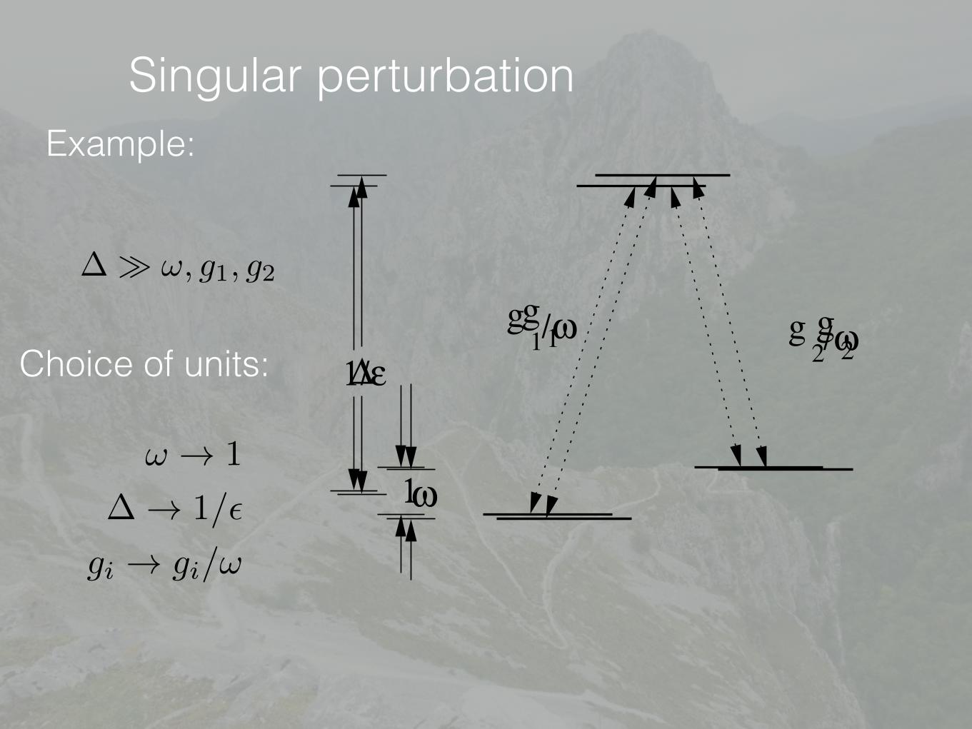
Singular perturbationExample:
2
ω
∆
g g1
� � !, g1, g2
Choice of units:
! ! 1
� ! 1/✏
gi ! gi/!
/ω
1
g1 21/ε
g /ω

Singular dynamical system
i↵̇ = �1
2↵+
g1!�
i�̇ =1
2� +
g2!�
i✏�̇ = � +✏
!(g1↵+ g2�)

Secular terms
First order perturbation
↵(t) = ↵(0)
✓1 + ✏
ig21t
!2
◆eit/2
+ ✏2ig1g2!2
�(0) sin(t/2) +O(✏2)
Secular Term

Singular perturbation techniques
• Multiple scales • Lindstet - Poincaré • Averaging • Dynamical Renormalisation Group • …
Our choice here:
Invariant manifold

Invariant manifold methodGiven a flow in a manifold, which are the submanifolds that are invariant under the flow….
… and can be determined perturbatively?Additional structure present, is it preserved in the embedding? !
Hamiltonian flow, e.g.

Translation to quantum mechanics
Schrödinger’s equation: i~@t = H
Invariance: existence of an operator (for Bloch) such that
B
HBH ✓ BHHB = BHB
Bloch equation
[H,B]B = 0
B2 = B ; B† 6= B

Further constraints
By itself, it is not very useful: Fully solving Bloch’s equation is equivalent to diagonalising the Hamiltonian
Need additional input for usefulness

Feshbach partitioning
Assume existence of projector P onto an uncoupled low energy sector
/ω
1
g1 21/ε
g /ω
P
Q = 1� P

Feshbach and BlochRestriction on the Bloch operator B
• Size of the subspace:
• Bloch-Feshbach alignment:
rank(B) = rank(P )
BP = B
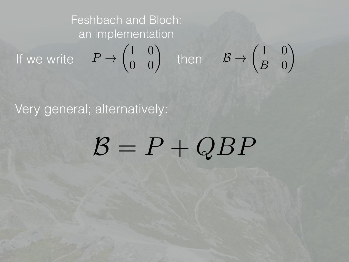
Feshbach and Bloch: an implementation
If we write P !✓1 00 0
◆then B !
✓1 0B 0
◆
Very general; alternatively:
B = P +QBP

Feshbach and Bloch: an implementation
Same basis,
H =
✓PHP PHQQHP QHQ
◆= ~
✓! ⌦†
⌦ �
◆
Bloch
[H,B]B = 0 , ⌦+�B = B! +B⌦†B

Separated energy scales
H = ~✓! ⌦†
⌦ �
◆with invertible � and
✏ = k��1k k!k ⌧ 1
✏0 = k��1k k⌦k ⌧ 1

Separated scales: equations of motion
Define ↵ = P
� = Q
Equations of motion:
Also ⌧ = k!kt
i@⌧↵ =!
k!k↵+⌦†
k!k�
i✏@⌧� = k��1k⌦↵+ k��1k��
= ✏⌦
k!k↵+ k��1k��Singular perturbation

Bloch operator and separated scales
Equation: ⌦+�B = B! +B⌦†B
Alternatively: B = ���1⌦+��1B! +��1B⌦†B
= T (B)
If scales are separated:
kT (A)k ✏0�1 + kAk2
�+ ✏kAk

Bloch operator and separated scales
kT (A)k ✏0�1 + kAk2
�+ ✏kAk
0.5 1.0 1.5 2.0 2.5 3.0
0.5
1.0
1.5
2.0
2.5
3.0
Iteration

Result (A)
If there is separation of scales there is a (small) solution of Bloch’s equation
which can be built iteratively or perturbatively
(small: )kBk = O(✏0)

Iteration/perturbationB(0) = 0
B(k+1) = ThB(k)
i
= ���1⌦+��1B(k)! +��1B(k)⌦†B(k)
B(0) = 0
B(1) = ���1⌦
B(2) = ���1⌦���2⌦! +��2⌦⌦†��1⌦

Iteration/perturbationB(1) = ���1⌦
B(2) = ���2⌦!
B(k+1) = ��1B(k) +��1k�1X
l=1
B(k�l)⌦†B(l)
B(1) = ���1⌦
B(2) = ���2⌦!
B(3) = ���3⌦! +��2⌦⌦†��1⌦
B(k) �kX
l=1
B(l) = O⇣��(k+1)
⌘

Result (B)
Resummation of the secular terms!
he↵ = ! + ⌦†B
i@t↵ = he↵↵

Effective hamiltoniansh(k)e↵ = ! + ⌦†B(k)
h(k)e↵ = ! +kX
l=1
⌦†B(l)
h(1)e↵ = ! � ⌦†��1⌦
h(2)e↵ = h(1)
e↵ + ⌦†��2⌦⌦†��1⌦
� ⌦†��2⌦!
Not hermitian!

Why not hermitian?Essentially, he↵ ⇠ PHB
Physically, =
✓↵B↵
◆
Carries a fraction of the norm
Total norm: † = ↵† �1 +B†B
�↵

Hermitian hamiltonian
hB =�1 +B†B
�1/2he↵
�1 +B†B
��1/2
is hermitian if a solution of Bloch’s equationB
• Similarity transformation • Isospectral • Induces approximations • Hermitian approximations?

Hermitian Hamiltonian If a solution of Bloch’s equationB
�1 +B†B
� �! + ⌦†B
�= ! + ⌦†B +B†⌦+B†�B
sohB =
�1 +B†B
�1/2he↵
�1 +B†B
��1/2
=1p
1 +B†B
�! + ⌦†B +B†⌦+B†�B
� 1p1 +B†B
amenable to hermitian approximations

Connection to other approaches
Equivalence to unitary transformations with perturbative exponents
X =
✓1 �B†
B 1
◆0
@1p
1+B†B0
0
1p1+BB†
1
A
= exp
arctanh
✓0 �B†
B 0
◆�
block diagonalises the hamiltonian, if solution of Bloch

Connection to other approaches
Interleaves projectors
XP = PXXwith exact projector onto the dressed low
energy sector
PX

Examples: Lambda system
2
ω
∆
g g1
20 40 60 80 100 120D t
0.2
0.4
0.6
0.8
1.0
p
Exacth(4)e↵
!

Examples: Lambda system
2
ω
∆
g g1
20 40 60 80 100 120D t
0.2
0.4
0.6
0.8
1.0
p
Exacth(4)e↵
h(10)B

Example: phenomenological time of arrival
H =p2
2m+
~⌦(x)2
�x
� ~ (2�(x) + i�)
4(1� �
z
)
Question: what is the effective evolution of the spatial wave function of the (1 0)T
component?

Example: phenomenological time of arrival
Bloch equation:
B =⌦
2�+ i�+
1
m~1
2�+ i�
⇥B, p2
⇤� 1
2�+ i�B⌦B
Conditions:• Small kinetic energy • Either detuning or
dissipation dominates over Rabi

Example: phenomenological time of arrival
Effective potential W =~2⌦B
Adiabatic approximations:
W
(1)(x) =~2
⌦2(x)
2�(x) + i�
W
(2)(x, p) = W
(1)(x)� ~2
⌦4(x)
(2�(x) + i�)3
� ~2m
⌦
2�+ i�
"~✓
⌦
2�+ i�
◆00+ 2i
✓⌦
2�+ i�
◆0p
#
Non local term

Conclusions
• Adiabatic elimination in quantum optics is another instance of a general structure
• Separation of energy scales leads to singular perturbation dynamical systems
• The invariant manifold method resums secular terms • Guaranteed existence of scale separated Bloch
operator • Explicit construction of hermitian effective
hamiltonians

Thank you!