additive models with spatio-temporal data
TRANSCRIPT

Environ Ecol StatDOI 10.1007/s10651-014-0283-6
Additive models with spatio-temporal data
Xiangming Fang · Kung-Sik Chan
Received: 7 July 2013 / Revised: 10 February 2014© Springer Science+Business Media New York 2014
Abstract Additive models (AMs) have been widely used in environmental, biolog-ical, and ecological studies. While the procedure for fitting an AM to independentdata has been well established, the currently available methods for fitting AMs withcorrelated data are not completely satisfactory in practice. We propose a new approachbased on penalized likelihood method to fit AMs for spatio-temporal data. Both maxi-mum likelihood and restricted maximum likelihood estimation schemes are developed.Conditions for asymptotic posterior normality are investigated for the case with fixedspatial correlation structure and no temporal dependence. We also propose a newmodel selection criterion for comparing AMs with and without spatial correlation.The proposed methods are illustrated by both simulation study and real data analysison the abundance distribution of Alaska plaice in eastern Bering Sea.
Keywords Additive models · Matérn model · Maximum likelihood · Penalizedlikelihood · Restricted maximum likelihood
1 Introduction
In geostatistics, modeling both the mean structure and the covariance structure is oftenof interest. When the mean relationships are complex and can not be easily modeled byspecific linear or non-linear functions, an additive model (AM) or generalized additive
Handling Editor: Ashis SenGupta.
X. Fang (B)Department of Biostatistics, East Carolina University, Greenville, NC 27834, USAe-mail: [email protected]
K.-S. ChanDepartment of Statistics and Actuarial Science, University of Iowa, Iowa City, IA 52242, USA
123
Environ Ecol Stat
model (GAM) can be a natural choice. Due to their flexibility in model specification,(generalized) AMs have seen a variety of applications. Examples include Hastie andTibshirani (1995), Lehmann (1998), Frescino et al (2001), Guisan et al (2002), andDominici et al (2002).
Much research has been devoted to fitting an AM/GAM with independent data usingspline methods (Wahba 1990; Green and Silverman 1994; Gu 2002; Wood 2006).However, only limited work has been done for correlated data. Several researchershave restricted their attention to longitudinal data with normally distributed responsesand have incorporated a nonparametric time function in linear mixed models (Zegerand Diggle 1994; Zhang et al 1998). Xue et al (2010) investigated GAMs for lon-gitudinal data. For more general cases, Lin and Zhang (1999) proposed generalizedadditive mixed models (GAMMs) which suffer from bias problems especially whenthe random effects are correlated. Wood (2006) included GAMMs in his R packagemgcv based on Lin and Zhang’s approach. He pointed out that GAMM fitting is not asnumerically stable as GAM fitting and will occasionally fail, especially when the corre-lation in the data is explicitly modelled, which is probably because of the confoundingbetween correlation and nonlinearity. Fahrmeir and Lang (2001) and Fahrmeir et al(2004) proposed a full Bayesian approach which estimates the mean structure andthe covariance parameters simultaneously. Since all inferences are based on MCMCsimulations, the computational cost of the Bayesian approach may be high, particu-larly when the sample size is large. Therefore, its practical feasibility deserves carefulconsideration.
We propose an alternative approach to fit an AM with correlated data via the penal-ized likelihood approach in the hope of avoding the complexity of the mixed modelapproach and the high computation cost of the Bayesian approach. Although the pro-posed approach does not assume any specific correlation structure, particular attentionwill be given to the spatial correlation defined by the Matérn class (Matérn 1986). TheMatérn class is a rich family of autocovariance functions taking the general form
K (h) = σ 2 (h/φ)ν
2ν−1Γ (ν)Kν(h/φ),
where h is the distance between two data points, σ 2 is the variance parameter, ν is thesmoothness parameter, φ is the range parameter, and Kν(x) is the modified Besselfunction of the second kind with order ν. The smoothness parameter ν controls thebehavior of the autocorrelation function for observations that are seperated by smalldistances. The Matérn class includes the exponential correlation function with ν = 0.5and the Gaussian correlation function as a limiting case when ν → ∞.
Some of the Matérn model parameters are not consistently estimable under fixeddomain asymptotics (Ying 1991; Stein 1999; Zhang 2004). What if we have repeatedmeasurements at the sampling locations? To answer this question, situations for thespatio-temporal data, where the spatial design is assumed to be fixed with temporallyindependent repeated measurements, are investigated by studying the conditions forasymptotic posterior normality. Data satisfying the aforementioned conditions areincreasingly collected in science, for example, large-scale annual fisheries monitoringdata; see Sect. 8.
123
Environ Ecol Stat
Statistical inference of the proposed methods will be developed based on the fact thatthe penalized likelihood function has a Bayesian interpretation: a function proportionalto the posterior density with some suitable prior. Asymptotic posterior normality hasbeen an important topic in Bayesian inference, see, e.g. Walker (1969) and Sweeting(1992). Here, we study conditions under which asymptotic posterior normality holdsin the spatio-temporal case. As temporal independence is a strong assumption ofour analysis, a model diagnosis method is developed to check the assumption ofindependence across time for the spatio-temporal data.
Our work is motivated by the needs for analyzing a set of spatio-temporal data onthe abundance of various fish species collected from the annual bottom trawl surveysin the eastern Bering Sea (EBS) since 1987 (see Sect. 8), although we shall only usedata on Alaska plaice (AP) for illustration. The availability of such large-scale spatio-temporal data affords a unique opportunity for assessing the possibly nonlinear effectsof environmental conditions on the spatial distribution of a fish species and the extentof the spatial correlation. Such knowledge provides valuable information for fisheriesmanagement of EBS fish stocks.
The rest of the paper is organized as follows. In Sect. 2, we introduce the AM withspatially correlated but temporally independent data. A detailed description of our newapproach for fitting AMs with correlated data is given in Sect. 3. In Sect. 4, conditionsfor asymptotic posterior normality under the spatio-temporal case are investigated. Asimulation study on the performance of the new approach is given in Sect. 5, and amodel diagnosis method for checking the assumptions of independence across timeis developed in Sect. 6. Also, we propose a model selection criterion based on theBayesian framework in Sect. 7 to compare different candidate models. Finally, theproposed methodology is applied to modeling the distribution of AP in the EBS, withthe main aim of exploring the environmental effects on the spatial distribution of APand the extent of spatial correlation.
2 A class of spatio-temporal models
Consider the AM
Yt = f1(x1t ) + f2(x2t ) + · · · + fm(xmt ) + et , t = 1, 2, 3, . . . , T (1)
where Yt ∈ Rn0 with n0 the number of observations from n0 sites for each time periodt (it is straightforward to extend to the case of non-constant number of sites); x j t arethe values of covariates x j at time t , and whose value at site s is denoted by x jt (s);f j (x j t ) denotes the vector consisting of f j (x jt (s)), s = 1, 2, . . . , n0 where f j areunknown smooth functions; et ∼ N (0, Σ t (θ)) with Σ t (θ) defined by some spatialcovariogram function K .
3 Parameter estimation
For simplicity, we describe our new fitting approach using a special case of Model (1)where t = m = 1, i.e., there are only one time period and one smooth function. The
123

Environ Ecol Stat
approach can be easily adapted for multiple smooth functions and multiple time-perioddata.
3.1 Model
Suppose the model is
Yi = f (xi ) + εi , i = 1, 2, . . . , n,
where xi is a d-vector of the covariates; f is a unknown smooth function with secondorder derivative; and the errors ε = (ε1, . . . , εn)′ have a multivariate normal distrib-ution with mean 0 and covariance matrix Σθ where θ are the covariance parameters.Consider the problem of estimating θ and f based on data Y = (Y1, Y2, . . . , Yn)′
and x =⎛⎝
x′1
. . .
x′n
⎞⎠. As in GAMs with uncorrelated errors, this goal can be achieved by
maximizing the penalized log likelihood
�P = −n
2log(2π) − 1
2log |Σθ | − 1
2(Y − f(x))′Σ−1
θ (Y − f(x)) − 1
2λJ ( f ), (2)
where f(x) = [ f (xi ), i = 1, . . . , n]′, λ is the smoothing parameter controlling thetradeoff between the model fit and the smoothness of the regression function, and Jis a roughness penalty functional (Wood 2006).
It is hard to maximize �P with respect to θ and f simultaneously. Therefore, we pro-pose an iterative algorithm which maximizes the penalized log likelihood alternativelywith respect to the covariance parameters and the smooth functions.
3.2 Penalized maximum likelihood estimation
The algorithm for covariance parameter estimation is as follows:Step 1 Start with some initial value of θ , say θ (0). One way to find an initial estimate ofθ is to fit a variogram model to the residuals from an AM assuming independent errors.Then treat θ as known and select the value of λ and estimate the smooth function f .
For fixed θ , maximizing (2) becomes
maxf
{−1
2(Y − f(x))′Σ−1
θ (Y − f(x)) − 1
2λJ ( f )
}.
It can be shown that for fixed θ the solution of f to the above maximization problemis a natural cubic spline if d = 1 and a natural thin-plate spline if d > 1 (Green andSilverman 1994). Thus f(x) can be represented as a linear function of the spline basis,i.e., f(x) = Xβ for some unknown parameters β and X is the design matrix of thespline basis function. Moreover, J ( f ) = β ′Sβ for some known symmetric matrix
123
Environ Ecol Stat
S, see Wood (2006). Hence the maximization problem is equivalent to the penalizedweighted least squares problem
minβ
{||Σ−1/2
θ (Y − Xβ)||2 + λβ′Sβ
}
ormin
β
{||Y − Xβ||2 + λβ
′Sβ
}(3)
where Σ−1/2θ is any square root matrix of Σ−1
θ such that(Σ
−1/2θ
)′Σ
−1/2θ = Σ−1
θ ,
Y = Σ−1/2θ Y and X = Σ
−1/2θ X.
The smoothing parameter can be estimated by a number of criteria, e.g. crossvalidation (CV) or generalized cross validation (GCV). Here, we shall estimate λ byminimizing the GCV
V = n||Y − AY||2[n − tr(A)]2
,
where A = X(X′X + λS)−1X′.With known θ and λ, the minimization problem (3) admits a unique solution, i.e.,
β = (X′X+λS)−1X′Y = (XΣ−1θ X+λS)−1X′Σ−1
θ Y, if XΣ−1θ X+λS is of full rank.
Denote the selected λ and the corresponding estimated β as λ(1) and β(1) respec-tively.Step 2 Let λ = λ(1) and β = β(1), and try to find a new estimate of θ .
With λ and β fixed, maximizing (2) becomes
maxθ
{−1
2(Y − Xβ)′Σ−1
θ (Y − Xβ) − 1
2log |Σθ |
}.
Clearly the solution is the MLE of θ with β(1) plugged in. Denote the new estimateof θ as θ (1).Step 3 Stop if ||θ (1)−θ (0)||
||θ (0)|| < 10−4. Otherwise, let θ (0) = θ (1) and repeat Steps 1–3.
Treating the penalty as a prior, the inference of the penalized maximum likelihood(ML) estimator will be based on the fact that the penalized likelihood, as proportionalto the posterior density of β and θ , asymptotically has an normal distribution thatcenters on the penalized likelihood estimator. This will be more carefully studiedbelow. For the moment, we outline the asymptotic inference procedures. Conditionalon the covariates, the standard errors of θ can be obtained based on the informationmatrix or the observed information matrix from the penalized log likelihood defined
by (2). Since E ∂2�P∂θ∂β ′ = 0, the Fisher information matrix can be verified to equal
I =(
X′Σ−1θ X + λS 0
0 −E ∂2�P∂θ∂θ ′
).
123

Environ Ecol Stat
Thus under some suitable regularity conditions (Wood 2006), it can be expected that,
β·∼ N
(β, (X′Σ−1
θ X + λS)−1)
and
θ·∼ N
(θ ,
(−E
∂2�P
∂θ∂θ ′)−1
).
The fitted smooth function f is given by Xβ. Now the covariance matrix of f equals
Var(f) = XVar(β)X′ = X(
X′Σ−1θ X + λS
)−1X′,
and we may thus construct (pointwise) confidence intervals (CIs) for the smoothfunction. If there are more than two smooth functions in the model, the correspondingsubmatrix of X, subset of β and submatrix of Var(β) can be used to estimate eachcomponent smooth function and construct CIs for each of them. Note that for themodel to be then identifiable, the model matrix and the estimated coefficients for anAM are for the centered smooth functions, which means each of the estimated smoothfunctions sums to zero across the data. (An intercept is implicitly included in a modelwith two or more smooth functions).
3.3 Penalized restricted maximum likelihood estimation
Maximum likelihood estimation tends to underestimate the covariance parameters,while the restricted maximum likelihood (REML) estimation is less biased (Corbeiland Searle 1976). For unpenalized likelihood, the restricted likelihood is the averageof the likelihood over all possible values of regression coefficients β, i.e.,
L R(θ) =∫
L(β, θ)dβ,
where β is given a non-informative prior.A penalized likelihood can be thought of as imposing some prior beliefs about the
likely characteristics of the correct model, which means we need to specify a priordistribution on β and θ . We assume that, given the smoothing parameter, θ has a flatprior over its parameter space Θ and is independent of β. Moreover, the (improper)prior of β equals
p(β|λ) = |D+|1/2
(2π)m/2 exp
{−1
2λβ ′Sβ
}
where m is the number of strictly positive eigenvalues of S and D+ is the diagonalmatrix with all those strictly positive eigenvalues of S arranged in descending order
123

Environ Ecol Stat
on the leading diagonal. This prior is appropriate since it makes explicit the belief thatsmooth functions are more likely than wiggly ones, but gives equal probability densityto all models of equal smoothness (see Wood 2006, page 190). In fact, the penaltyterm in the penalized likelihood corresponds to this prior.
With the prior given above, the restricted penalized likelihood function equals
L R(θ |Y) =∫
f (Y|β, θ)p(β|θ)dβ
= |D+|1/2
(2π)(n+m)/2|Σθ |1/2exp
{−1
2(Y − Xβ)′(Y − Xβ)
}√(2π)p
|X′X|
where Y =(
Σ−1/2θ Y
0
), X =
(Σ
−1/2θ XB
), β = (X′X)−1X′Y, p = dim(β), and
B is any matrix such that B′B = λS. After some algebra, the penalized restrictedlog-likelihood function can be expressed as
�R(θ |Y) = log L R(θ |Y)
∝ −1
2log(|Σθ |) − 1
2log
(|X′Σ−1
θ X + λS|)
−1
2Y′
[Σ−1
θ − Σ−1θ X
(X′Σ−1
θ X + λS)−1
X′Σ−1θ
]Y.
Penalized restricted likelihood estimation can then be carried out iteratively using ascheme similar to that for ML estimation, except that Step 2 is modified as follows:With fixed λ, maximizing �R with respect to θ gives the REML estimate θ (1). Steps 1and 3 are exactly the same as before. Also, the standard errors of the REML estimatorand the CIs for θ can be obtained based on the information matrix from the penalizedrestricted log likelihood.
4 Asymptotic posterior normality
As described in the previous section, given a fixed set of basis functions, model (1)can be rewritten as
Yt = Xtβ + et , t = 1, 2, 3, . . . , T, (4)
and the corresponding penalized log likelihood equals
�P =−T · n0
2log(2π) − T
2log |Σθ | − 1
2
T∑t=1
(Yt − Xtβ)′Σ−1θ (Yt − Xtβ) − 1
2β ′Sβ.
Note that the smoothing parameters are assumed known and hence absorbed into thematrix S.
For fixed smoothing parameters, the maximum penalized likelihood estimator canbe interpreted as the posterior mode under a suitable prior density. Recall the jointprior density of β and θ is given by
123

Environ Ecol Stat
p(β, θ) = |D+|1/2
(2π)m/2 exp
{−1
2β ′Sβ
}. (5)
Hence the posterior density equals
p(β, θ |data) = p(β, θ)p(Y|β, θ)/∫
p(Y|β, θ)p(β, θ)dβdθ
=|D+|1/2 exp
{− 1
2
∑Tt=1(Yt − Xtβ)′Σ−1
θ (Yt − Xtβ) − 12β ′Sβ
}
(2π)(m+T ·n0)/2|Σθ |T/2∫
p(Y|β, θ)p(β, θ)dβdθ
(6)
which is exactly the penalized likelihood up to a normalization constant. Note that theanalysis in this section is also conditional on the design matrix X.
Below, we state a theorem on the asymptotic posterior normality for AMs underthe spatio-temporal setting where the spatial design does not change over time, i.e.,Σ t (θ) = Σθ for all t , and the random errors are temporally independent, i.e.,τ(|t1 − t2|) = 1 if t1 = t2 and 0 otherwise. Thus the random vectors et1 and et2are independent for t1 �= t2. The proof is provided in the appendix. The temporalindependence assumption is a strong assumption. We will study the issue of checkingthe validity of this assumption later.
Theorem 1 Consider the spatio-temporal model (4) with fixed spatial design andtemporally independent data. Let φ0 = (β0, θ0) ∈ Φ = Rk ×Θ be the true parametervalue, where Θ is a relatively compact, open convex subset of Rl . Suppose the priorfor φ = (β, θ) ∈ Φ is defined by (5), the covariogram function K (·|θ) is twicedifferentiable w.r.t. θ , and the covariance matrix Σθ is invertible and continuous overΘ . Furthermore, assume the following conditions are satisfied:
(A1) for fφ(Yt ) = − ∂2l(φ|Yt )
∂φφ′ , ∃ δ0 > 0 and a finite, integrable function M(Yt ) such
that sup|φ−φ0|<δ0
∥∥ fφ(Yt )∥∥
max ≤ M(Yt ) where ‖ · ‖max is the maximum norm;
(A2) for fθ (et ) =(
∂
∂θ′ X
′tΣ
−1θ
)et , ∃ δ1 > 0 and a finite, integrable functions M1(et )
such that sup|θ−θ0|<δ1‖ fθ (et )‖max ≤ M1(et );
(A3) 1T
∑Tt=1
∂∂θ
X′tΣ
−1θ Xt is bounded, uniformly for θ ∈ Θ in probability;
(A4) over the closure of Θ , − 1T
∂2l(φ)
∂θ∂θ ′ is positive definite and a continuous functiona.s.;
(A5) infθ∈Θ λmin
(1T
∑Tt=1 X
′tΣ
−1θ Xt
)> 0 a.s., where λmin(A) denotes the mini-
mum eigenvalue of a symmetric matrix A.
Then there exists a sequence of local maxima of the posterior density defined by (6)
aroundφ0 such that the posterior density of(
J1/2T
)′ (φ − φT
)converges in probability
123
Environ Ecol Stat
to the standard multivariate normal distribution, where J1/2T is the left Cholesky square
root of JT =[
JT (β) 00 JT (θ)
]with the diagonal blocks
JT (β) =T∑
t=1
XtΣ−1θ
Xt + S
and
JT (θ) = −∂2l(φ)
∂θ∂θ ′∣∣∣β=β,θ=θ
.
Several remarks are in order. Note that this theorem implies that the (normalized)penalized likelihood function asymptotically approaches the normal density with meanφT and variance matrix J−1
T . Recall that in Sect. 3, the variance matrix of θ is given by
the inverse negative Hessian matrix w.r.t. θ and the variance matrix of β is given by
the posterior variance(
X′Σ−1θ
X + S)−1
which is also the inverse negative Hessian
matrix w.r.t. β. Therefore, this theorem provides a justification, in the case of spatio-temporal model, of the way that inferential procedures of β and θ are outlined inSect. 3.
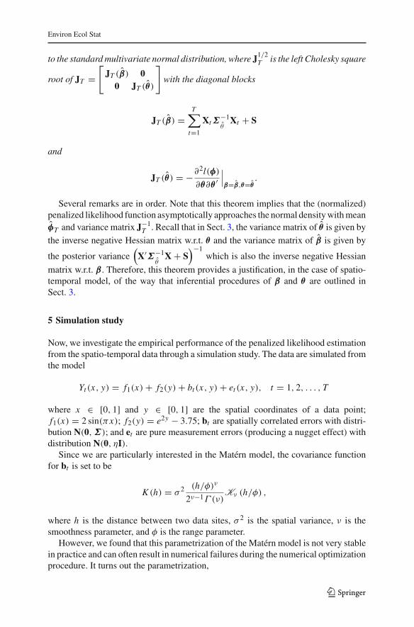
5 Simulation study
Now, we investigate the empirical performance of the penalized likelihood estimationfrom the spatio-temporal data through a simulation study. The data are simulated fromthe model
Yt (x, y) = f1(x) + f2(y) + bt (x, y) + et (x, y), t = 1, 2, . . . , T
where x ∈ [0, 1] and y ∈ [0, 1] are the spatial coordinates of a data point;f1(x) = 2 sin(πx); f2(y) = e2y − 3.75; bt are spatially correlated errors with distri-bution N(0,Σ); and et are pure measurement errors (producing a nugget effect) withdistribution N(0, ηI).
Since we are particularly interested in the Matérn model, the covariance functionfor bt is set to be
K (h) = σ 2 (h/φ)ν
2ν−1Γ (ν)Kν (h/φ) ,
where h is the distance between two data sites, σ 2 is the spatial variance, ν is thesmoothness parameter, and φ is the range parameter.
However, we found that this parametrization of the Matérn model is not very stablein practice and can often result in numerical failures during the numerical optimizationprocedure. It turns out the parametrization,
123

Environ Ecol Stat
Table 1 Covariance parameter estimation
Sample True value ML REML
Mean Median SD SD* Mean Median SD SD*
100 × 1 σ 2 = 1 0.520 0.477 0.229 0.208 34.88 0.991 291.7 0.772
υ = 2 4.349 4.118 2.606 2.222 3.087 2.555 2.453 2.510
ρ = 0.045 0.028 0.010 0.056 0.012 10.19 0.028 125.1 0.115
η = 0.1 0.090 0.092 0.036 0.032 0.088 0.091 0.038 0.034
400 × 1 σ 2=1 0.581 0.527 0.251 0.208 9.266 0.947 137.8 0.572
υ = 2 3.200 3.023 1.459 1.318 2.302 2.075 1.123 1.083
ρ = 0.045 0.027 0.017 0.028 0.014 4.315 0.042 108.0 0.050
η = 0.1 0.101 0.101 0.010 0.010 0.099 0.100 0.011 0.011
100 × 5 σ 2=1 0.903 0.900 0.155 0.146 1.002 0.999 0.176 0.169
υ = 2 2.358 2.165 0.900 1.006 2.210 2.020 0.849 0.931
ρ = 0.045 0.046 0.038 0.032 0.028 0.053 0.044 0.036 0.032
η = 0.1 0.099 0.100 0.015 0.014 0.099 0.099 0.015 0.015
100 × 10 σ 2=1 0.949 0.951 0.106 0.112 1.000 1.004 0.113 0.123
υ = 2 2.174 2.137 0.590 0.512 2.117 2.081 0.576 0.506
ρ = 0.045 0.046 0.040 0.026 0.018 0.049 0.043 0.027 0.019
η = 0.1 0.100 0.100 0.011 0.010 0.099 0.100 0.011 0.009
K (h) = σ 2
(hνρ
)ν
2ν−1Γ (ν)Kν
(h
νρ
),
where ρ = φ/ν, performs much better numerically. From now on, we will use thisnew parameterization of the Matérn model. So the parameters of interest here areθ = (σ 2, ν, ρ, η)′.
The random fields bt are independently simulated on the same set of locationsand from the same normal distribution N(0, Σ) where Σ is defined by the Matérncovariogram with σ 2 = 1, ν = 2, ρ = 0.045. The measurement errors et aresimulated from the normal distribution N(0, ηI) where η = 0.1. There are 100locations, so the total sample size is 100 × T . The fitting results, which are basedon 1,000 replicates for T = 1, 500 for T = 5 and 200 for T = 10, are shown inTables 1 and 2. As extremely large and extremely small estimates can be producedin estimating the covariance parameters, in addition to the sample means and samplestandard deviations we also include the medians and values of a more robust standarddeviation SD* to summarize the simulation results. Let IQR denote the interquartilerange. The robust standard deviation SD* = IQR/1.349, which estimates the standarddeviation if data are normally distributed. To evaluate the estimation of the smoothfunctions, we calculated the mean square errors of the fitted functions and the 95 % CIcoverage proportion, which is the proportion of data points that are covered by their95 % CIs.
123
Environ Ecol Stat
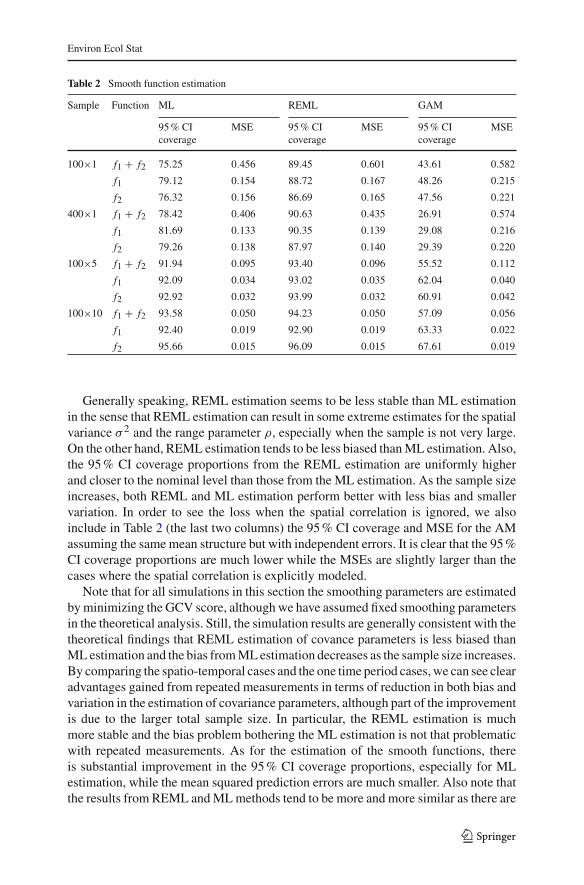
Table 2 Smooth function estimation
Sample Function ML REML GAM
95 % CIcoverage
MSE 95 % CIcoverage
MSE 95 % CIcoverage
MSE
100×1 f1 + f2 75.25 0.456 89.45 0.601 43.61 0.582
f1 79.12 0.154 88.72 0.167 48.26 0.215
f2 76.32 0.156 86.69 0.165 47.56 0.221
400×1 f1 + f2 78.42 0.406 90.63 0.435 26.91 0.574
f1 81.69 0.133 90.35 0.139 29.08 0.216
f2 79.26 0.138 87.97 0.140 29.39 0.220
100×5 f1 + f2 91.94 0.095 93.40 0.096 55.52 0.112
f1 92.09 0.034 93.02 0.035 62.04 0.040
f2 92.92 0.032 93.99 0.032 60.91 0.042
100×10 f1 + f2 93.58 0.050 94.23 0.050 57.09 0.056
f1 92.40 0.019 92.90 0.019 63.33 0.022
f2 95.66 0.015 96.09 0.015 67.61 0.019
Generally speaking, REML estimation seems to be less stable than ML estimationin the sense that REML estimation can result in some extreme estimates for the spatialvariance σ 2 and the range parameter ρ, especially when the sample is not very large.On the other hand, REML estimation tends to be less biased than ML estimation. Also,the 95 % CI coverage proportions from the REML estimation are uniformly higherand closer to the nominal level than those from the ML estimation. As the sample sizeincreases, both REML and ML estimation perform better with less bias and smallervariation. In order to see the loss when the spatial correlation is ignored, we alsoinclude in Table 2 (the last two columns) the 95 % CI coverage and MSE for the AMassuming the same mean structure but with independent errors. It is clear that the 95 %CI coverage proportions are much lower while the MSEs are slightly larger than thecases where the spatial correlation is explicitly modeled.
Note that for all simulations in this section the smoothing parameters are estimatedby minimizing the GCV score, although we have assumed fixed smoothing parametersin the theoretical analysis. Still, the simulation results are generally consistent with thetheoretical findings that REML estimation of covance parameters is less biased thanML estimation and the bias from ML estimation decreases as the sample size increases.By comparing the spatio-temporal cases and the one time period cases, we can see clearadvantages gained from repeated measurements in terms of reduction in both bias andvariation in the estimation of covariance parameters, although part of the improvementis due to the larger total sample size. In particular, the REML estimation is muchmore stable and the bias problem bothering the ML estimation is not that problematicwith repeated measurements. As for the estimation of the smooth functions, thereis substantial improvement in the 95 % CI coverage proportions, especially for MLestimation, while the mean squared prediction errors are much smaller. Also note thatthe results from REML and ML methods tend to be more and more similar as there are
123

Environ Ecol Stat
more repeated measurements, although for small to moderately large sample size theREML method generally has less bias and coverage rates closer to the 95 % nominallevel than the ML method. All these results imply that the AM with Matérn correlationstructure is much more tractable in the spatio-temporal case than the one-time-periodcase.
6 Checking temporal independence
So far, we have assumed that data are temporally independent. Next, we propose anapproach to check the validity of this assumption. Again, consider the spatio-temporalmodel defined by Eq. (1) with fixed spatial design. We assume that the temporalcorrelation and the spatial correlation are separable, i.e., the covariance of observationsat time t1, location s1 and time t2, location s2 can be written as
Cov(Yt1(s1), Yt2(s2)
) = Cov(et1(s1), et2(s2)
) = τ(|t1 − t2|)K (|s1 − s2|)
where τ is a temporal autocorrelation function (the temporal variance has beenabsorbed into K (|s1 − s2|). In other words, the temporal correlation scheme is inde-pendent of the spatial correlation scheme.
Let s1, s2, . . . , sn0 be the spatial locations and et (s) be the error term at location sand time t . Define et ≡ 1
n0
∑sn0s=s1 et (s). Then
Cov(et1 , et2
) = 1
n20
Cov
⎛⎝
sn0∑u=s1
et1(u),
sn0∑v=s1
et2(v)
⎞⎠
= τ(|t1 − t2|)∑sn0
u=s1
∑sn0v=s1 K (|u − v|)
n20
(7)
Since∑sn0
u=s1
∑sn0v=s1 K (|u−v|)n2
0is constant over time, Cov
(et1 , et2
)retains the temporal
correlation structure of the data. Therefore, it is reasonable to check the assumptionof independence across time by checking if there is autocorrelation among {εt , t =1, 2, . . . , T }, where εt is the average residual over all sampling locations at time t .
Note that the above argument is approximately correct even if the spatial locationsare not fixed over time provided that the number of sites is large and the sites arewell spread out. To see this, suppose s1, s2, . . . , sn0 are iid with density function h(s).Then (7) converges to τ(|t1 − t2|)
∫ ∫K (|u − v|)h(u)h(v)dudv as n0 → +∞. As∫ ∫
K (|u − v|)h(u)h(v)dudv does not depend on time, Cov(et1 , et2) still retains thetemporal correlation structure of the data.
7 Model selection
We propose a model selection criterion based on the marginal likelihood or evidence,which selects the model that asymptotically has the highest posterior probability,
123
Environ Ecol Stat
assuming uniform model prior probabilities. As before, we shall treat the penalty assome prior information. The analysis will be conditional on the estimated smoothingparameters which are henceforth treated as fixed numbers throughout this section. Forspatially correlated data, the exact marginal likelihood is generally intractable. (It,however, admits a closed-form solution for the case of independent, Gaussian data).We use the Laplace approximation (Tierney and Kadane 1986; Wong 1989) to derivean approximate formula for the marginal likelihood.
7.1 Additive models with correlated data—ML estimation
For simplicity, we consider the case of an AM with spatially correlated data and noreplication. Extension to the case of multi-yearly data is straightforward. The modelcan be rewritten as
Y = Xβ + e,
where e ∼ N (0,Σθ ) and θ ∈ Θ is the vector of the covariance parameters. Thepenalized log likelihood equals
−1
2log |Σθ | − 1
2(Y − Xβ)′Σ−1
θ (Y − Xβ) − 1
2β ′Sβ.
Note that the smoothing parameters are absorbed into the matrix S. Recall the jointprior density for β and θ is given by (5). The marginal likelihood of the model thenequals
∫p(y|β, θ)p(β, θ)dβdθ =
∫p∗(β, θ)dβdθ
where
p∗(β, θ) = |D+|1/2
(2π)(n+m)/2|Σθ |1/2exp
{−1
2(y − Xβ)′Σ−1
θ (y − Xβ) − 1
2β ′Sβ
}.
Let
�p∗ ≡ log p∗(β, θ)
= −n + m
2log(2π) + 1
2log |D+| − 1
2log |Σθ |
−1
2(y − Xβ)′Σ−1
θ (y − Xβ) − 1
2β ′Sβ,
and
Λ = − ∂2�p∗
∂(β, θ)∂(β, θ)′|β=β,θ=θ
=[
X′Σ−1θ X + S − ∂
∂θ ′ X′Σ−1θ (y − Xβ)
− ∂∂θ
(Y − Xβ)′Σ−1θ X − ∂2�p∗
∂θ∂θ ′
]
β=β,θ=θ .
123
Environ Ecol Stat
Since E[
∂∂θ ′ X′Σ−1
θ (y − Xβ)]
= 0, the off-diagonal blocks of Λ can be approximated
by 0 as β is close to the true value.By Laplace’s method, the marginal likelihood of the model equals
E ≡∫
p∗(β, θ)dβdθ ≈ p∗(β, θ)
√(2π)k+l
|Λ|
=√
(2π)k+l |D+|(2π)n+m |Σ
θ||Λ| exp
{−1
2(y − Xβ)′Σ−1
θ(y − Xβ) − 1
2β
′Sβ
}
where k = dim(β) and l = dim(θ). Hence, the log marginal likelihood equals
logE ≈ −n − m + k + l
2log(2π) + 1
2log |D+| − 1
2log |Σ
θ|
−1
2log |Λ| − 1
2(y − Xβ)′Σ−1
θ(y − Xβ) − 1
2β
′Sβ.
For the case of AM without spatial correlation, the log marginal likelihood is obtainedas above but with θ reduced to a single variance parameter and �
θreplaced by a
diagonal matrix.
7.2 Additive models with correlated data—REML estimation
In the previous section, we applied the Laplace method to the (β, θ) parameterizationwhich generally operates on a very high-dimensional parameter space as the dimensionof β is usually high. A more accurate approximation may be obtained by first inte-grating out β from the posterior density before applying the Laplace approximation,which yields the following approximation:
logE ≈ k + l − n − m
2log(2π) + 1
2log |D+| − 1
2log |Σ
θ|
−1
2log |Λ| − 1
2log |X′Σ−1
θX + S|
−1
2y′ [Σ−1
θ− Σ−1
θX(X′Σ−1
θX + S)−1X′Σ−1
θ
]y,
where k = dim(β), l = dim(θ), and Λ = − ∂2�p∗∂θ∂θ ′ |θ=θ
; here θ is the REML estimatorof θ and
�p∗ = −n − m + k
2log(2π) + 1
2log |D+| − 1
2log |X′Σ−1
θ X + S|
−1
2log |Σθ | − 1
2y′ [Σ−1
θ − Σ−1θ X(X′Σ−1
θ X + S)−1X′Σ−1θ
]y.
123

Environ Ecol Stat
7.3 Simulation study
Although the model selection criteria derived in the previous section can be usedto compare nested or non-nested models, we are particularly interested in choosingbetween AMs with and without spatial correlation in this simulation study. For thespatially correlated AM, we simulated data from the model
Y (x, y) = f1(x) + f2(y) + b(x, y) + e(x, y),
where x ∈ [0, 1] and y ∈ [0, 1] are the spatial coordinates of a data point; f1(x) =1+2x ; f2(y) = −3y; b is the spatially correlated error with Matérn covariogram withσ 2 = 1, ν = 2, ρ = 0.045; and e is the pure measurement error from the normaldistribution with mean 0 and variance η varied from 0.1, 0.5, 1 and 10. The samplesize is 200. We also simulated data from the AM with the same mean structure butwith spatially independent noise, i.e., b is absent but η ranges from 1.1, 1.5, 2 and 11to match the overall noise variance of the spatially correlated AM.
We analyze each simulated dataset in three ways: (1) an AM assuming independentdata; (2) an AM assuming Matérn-correlated data by ML estimation; and (3) an AMassuming Matérn-correlated data by REML estimation. The log marginal likelihoodis calculated for each case denoted by logE.gam, logE.ml or logE.reml respectively.The above procedure is repeated 500 times independently. Table 3 displays the relativefrequencies that the criterion of maximum marginal model probability picks the truemodel, i.e., logE.gam is greater than logE.ml and logE.reml for the independent datacases and vice versa for the correlated data cases. When the data are actually inde-pendent and we fit an AM with spatial correlation, the fitting procedure tends to failbecause the Matern covariogram is non-identifiable. When the estimation of the cor-related AM fails while that of the independent AM succeeds, we count the logE.gamas the largest value since logE.ml and logE.reml are missing.
It can be seen that the proposed criterion works well in picking the correct modelfor the independent data. For the correlated data, the criterion also has a good chanceof selecting the true model, especially when the nugget is relatively small comparingto the spatial variance. As the nugget η increases, the proposed criterion has a slightlybetter chance of selecting the true model when the data are independent and a lowerchance to pick the true model when the data are correlated. This is, however, expected.As the nugget increases, the spatial correlation is increasingly irrelevant and thus
Table 3 Proportion of times that the proposed criterion selects the true model
Variance η = 1.1 η = 1.5 η = 2 η = 11
Independent data P(logE.gam>logE.ml) 0.756 0.794 0.822 0.868
P(logE.gam>logE.reml) 0.792 0.798 0.832 0.866
Nugget η = 0.1 η = 0.5 η = 1 η = 10
Correlated data P(logE.ml>logE.gam) 0.954 0.680 0.626 0.360
P(logE.reml>logE.gam) 0.968 0.824 0.738 0.356
123

Environ Ecol Stat
Table 4 Proportion of times that the proposed criterion selects the true model: spatio-temporal data
Sample distribution 200 × 1 50 × 4 20 × 10 200 × 2
Independent P(logE.gam>logE.ml) 0.756 0.850 0.862 0.788
Data P(logE.gam>logE.reml) 0.792 0.854 0.840 0.796
Correlated P(logE.ml>logE.gam) 0.954 0.920 0.810 0.998
Data P(logE.reml>logE.gam) 0.968 0.930 0.796 1
increasingly difficult to detect. For the extreme case where the nugget is ten times ofthe spatial variance, the data are actually more like independent data and we have onlyabout one third chance of selecting the true model. Also, it seems the estimation method(ML or REML) has little effect on model selection when the data are independent,but for correlated data, REML estimation seems to result in a more effective modelselection criterion.
Next, we extend the simulation to include spatio-temporal data from an AM with thesame smooth functions given above. The errors are independent across different timeperiods, but either spatially correlated or spatially independent within each time period.With fixed spatial design, temporally independent repeated measurements are taken ateach location such that the total sample size is still 200. For all the spatially correlateddata, the parameters of the Matérn covariogram are σ 2 = 1, ν = 1, ρ = 0.045 withnugget 0.1. For the spatially independent data, the error variance is 1.1.
Table 4 shows the results, which are again based on 500 replicates. In general, theproposed criterion performs well with at least 75 % chance of success in picking thecorrect model for all the cases studied here. The criterion works particularly well whenthe data are spatially correlated. Even for the case with only 20 fixed data sites, theproposed criterion can select the true model about 80 % of the time. As there are morerepeated measurements with total sample size fixed, the criterion gains power fromrepeated measurements for the independent data, but for the spatially correlated data,the performance of the criterion gets relatively worse. This may be due to two possiblereasons. First, the temporal independence of the data could eliminate some spatialcorrelation comparing to the one-period case. Second, as the sample size per timeperiod decreases, there is some information loss in estimating the mean structure. Thebenefit from repeated measurements can be clearly seen for the correlated data whencomparing the 200 × 1 and the 200 × 2 cases. It is interesting to note that there is nosubstantial improvement for the independent data when adding one more observationat each location. Actually, this phenomenon holds even if the spatial design is randomacross time periods (results unreported).
8 Case study
Since 1979, the Resource Assessment and Conservation Engineering Division (RACE)of the Alaska Fisheries Science Center conducts annual bottom trawl survey in the EBSfor monitoring the condition of demersal fish and crab stocks in the EBS continentalshelf; see Acuna and Kotwicki (2006). These annual surveys generally covered a
123

Environ Ecol Stat
-175 -170 -165 -160
5456
5860
62Fitted Values of log(CPUE)
Longitude
Latit
ude
-2
-1
0
1
2
3
4
Contour Plot of s(x)+s(y)
Longitude
Latit
ude
-1
-1
-1
-0.50
0 0.5
0.5
1
1
1.5
-175 -170 -165 -160
5658
6062
200 400 600 800 1000 1200
-6-4
-20
2
x
s(x,
8.24
)
6200 6400 6600 6800
-6-4
-20
2y
s(y,
7.82
)
0 2 4 6 8 10
-6-4
-20
2
SURF_TEMP
s(S
UR
F_T
EM
P,1
.25)
-2 0 2 4 6 8
-6-4
-20
2
BOTTOM_TEMP
s(B
OT
TO
M_T
EM
P,4
.99)
50 100 150 200
-6-4
-20
2
DEPTH
s(D
EP
TH
,6.3
5)
1 2 3 4 5 6 7
-6-4
-20
2
phi
s(ph
i,8.6
5)
1985 1990 1995 2000 2005
-6-4
-20
2
YEAR
s(Y
EA
R,1
)
140 160 180 200 220
-6-4
-20
2
DATE
s(D
AT
E,1
)
Fig. 1 Estimated smooth functions (REML)
major portion of the EBS that included 395 sampling sites (See the upper-left panel ofFig. 1 for the sampling region). Sampling was done by trawling for 30 min at stationscentered in a 20×20 nautical mile grid covering the survey area. At each station, speciescomposition of the catch was determined. Here, we study the abundance distribution
123

Environ Ecol Stat
of the AP, a kind of flatfish, using the bottom trawl survey data from 1985 to 2007. Forsimplicity, we only focus on the spatio-temporal distribution of adult male AP withlength >273 mm.
The response variable is the AP abundance at a sampling site, which is measuredby catch per unit effort (CPUE). The explanatory variables of interest include the sam-pling position defined by longitude and latitude, the bottom depth in meters (DEPTH),sea surface temperature (SURF_TEMP), bottom temperature (BOTTOM_TEMP),smoothness of the bottom (phi) which is defined as the negative base-2 log of meangrain size, Julian day of sampling (DATE), and the year of sampling (YEAR). Sam-ples with zero density or missing values in any variable were removed, resulting in atotal of 3,763 data points left for the analysis. The log transformation was applied tothe response variable to normalize the distribution and reduce heteroscedasticity. Thelongitude and latitude are in degrees. In order to make it easier to interpret the distance,the locations are transformed into the Universal Transverse Mercator (UTM) coordi-nate system in kilometers such that the distance between two sites is their geodesicdistance.
We assume that data from different years are independent after the year effecthas been accounted for by a smooth function in the mean structure. Specifically, letYt (x, y) be the natural logarithm of CPUE at UTM location (x, y) in year t . Then theproposed model can be written as
Yt (x, y) = s1(x) + s2(y) + s3(DEPTH(x,y))
+ s4(SURF_TEMP(x,y)) + s5(BOTTOM_TEMP(x,y))
+ s6(phi(x,y)) + s7(DATEt ) + s8(YEARt )
+ bt (x, y) + et (x, y), (8)
where si are unknown smooth functions of the covariates, bt are the spatially correlatederrors with distribution N(0,Σ), and et are the independent measurement errors withdistribution N(0, ηI).
First, an AM assuming (spatially and temporally) independent errors is fitted (i.e.,bt (x, y) is ignored). Figure 2a shows the variogram of the fitted residuals, whichindicates that there is spatial correlation among the residuals. Thus an AM with inde-pendent errors seems to be inadequate for the data. We have also fitted a similar modelwith non-additive mean spatial effects where the additive functions s1(x)+s2(y) in (8)are replaced by s(x, y). However, the residuals still appear to be spatially correlated.As the use of non-additive mean spatial effects [i.e., the unknown smooth functions(x, y)] may confound with spatial correlation, henceforth we restrict the analysis tothe mean function defined by (8).
Then we fit an AM with spatially correlated, but temporally uncorrelated errorsusing both ML and REML estimation. We employed the Matérn covariogram formodeling the spatial correlation. For the ML estimation, the covariance parameters
with standard errors in parentheses are estimated to be σ 2 = 0.859 (0.224), ν = 0.765(0.461), ρ = 45.318 (37.314) and η = 0.526 (0.221). Their REML counterparts
are given by σ 2 = 0.862, (0.201), ν = 0.794 (0.447), ρ = 45.310 (35.336) andη = 0.555 (0.198). Note that the estimates from the two estimation methods are quite
123

Environ Ecol Stat
0 100 200 300 400 500
0.0
0.5
1.0
1.5
Variogram of Residuals
Distance
Sem
ivar
iogr
am(a) Additive model assuming spatially independent errors
0 100 200 300 400 500
0.0
0.5
1.0
1.5
Variogram of Residuals
Distance
Sem
ivar
iogr
am
0 100 200 300 400 5000.
00.
51.
01.
5
Variogram of Standardized Residuals
Distance
Sem
ivar
iogr
am
(b) Additive model assuming spatially correlated errors: ML Estimation
0 100 200 300 400 500
0.0
0.5
1.0
1.5
Variogram of Residuals
Distance
Sem
ivar
iogr
am
0 100 200 300 400 500
0.0
0.5
1.0
1.5
Variogram of Standardized Residuals
Distance
Sem
ivar
iogr
am
(c) Additive model assuming spatially correlated errors: REML Estimation
Fig. 2 Variograms of residuals
close, which is consistent with the simulation results in Sect. 5 when there is a largenumber of time periods. The variograms of the standardized residuals (see Fig. 2b, c)are fairly flat, which suggests that the Matérn covariogram has adequately explainedalmost all the spatial correlation and the standardized residuals are approximatelyindependent. For the three fits mentioned above, the log marginal likelihoods arerespectively log E.gam = −6, 103.961, log E.ml = −5, 915.503, log E.reml =−5, 864.719, which indicates that the models with spatial correlation are preferredand REML estimation is slightly better than ML estimation.
The estimated smooth functions are shown in Fig. 1. There is not much differencein the estimated smooth functions between the ML and REML estimation methods,hence only the REML estimates are shown in Fig. 1. The upper-left panel showsthe image plot of the fitted values of log(CPUE) which captures very well the majorpattern of the observed values (not shown in the figure). All the smooth terms otherthan surface temperature and the year effect are highly significant. In general, we foundthe following relationships between the explanatory variables and the abundance ofAP. (1) The surface temperature has no significant effect on the abundance distribution
123

Environ Ecol Stat
Table 5 p values of Ljung–Box test for temporal independence
Method lag 1 lag 2 lag 3 lag 4 lag 5 lag 6
ML 0.617 0.464 0.638 0.791 0.783 0.624
REML 0.620 0.458 0.636 0.789 0.782 0.635
after bottom temperature and bottem depth are taken into account. (2) Male APs seemto like relatively cold environment. There were more male adult APs at locations wherethe bottom temperature is around 0 ◦C. The abundance tends to decrease as bottomtemerature increases. (3) There were more male APs at loctions with the bottom deptharound 50 m. As the ocean gets deeper, the abundance of AP tends to decrease. (4)There were more male APs at locations where the bottom is not too smooth or toorough (phi is between 3 and 5). (5) There was no significant difference in the abundanceof APs from year to year during the period of the study. (6) There were less male adultAPs on early sampling days and more on late days. Besides the seasonal effect, thismay be an artifact of the traveling route of the cruises.
So far, we have assumed temporal independence. To check this assumption, theLjung–Box test (Ljung and Box 1978) is used to test for independence in spatiallyaveraged residuals. The Ljung–Box test statistic is Q = T (T + 2)
∑sk=1 r2
k /(T − k),where T is the number of observations, s is the number of coefficients to test forautocorrelation, and rk is the autocorrelation coefficient (for lag k). If the samplevalue of Q exceeds a critical value from a Chi-square distribution with s degrees offreedom, then at least one value of rk is statistically different from zero at the specifiedsignificance level. The Null Hypothesis is that none of the autocorrelation coefficientsup to lag s are different from zero. The test p-values for a maximum lag up to 6 areshown in Table 5. All the p values are >0.45, which lends support to the temporalindependence assumption for the AP data.
9 Conclusion and discussion
In this paper, we developed a new approach to fit AMs with correlated data, as analternative to the numerically less stable GAMM framework and the computationallyexpensive Bayesian method. Meanwhile, we also studied the properties of the Matérncorrelation model under the AM framework. In general, REML estimation tends tobe better than ML in terms of bias and CI coverage for the smooth functions, but MLestimation of the covariance parameters is more stable. However, it can be expected thatthe two methods tend to perform similarly when the sample size is large enough. Thevariations of the estimates sometimes seem to be large, but this is not surprising. Manyauthors have reported difficulties in likelihood estimation of covariance parameters(Mardia and Watkins 1989; Diggle et al 1998; Zhang 2002). In many parts of thispaper, we assume the random errors are temporally independent, which is a strongassumption. However, the temporal correlation can often be mostly accounted for byincluding a smooth function of time in the mean structure. Then the random errors canbe reasonably assumed to be temporally independent. Our experience with the annual
123

Environ Ecol Stat
fisheries data suggests this is usually the case unless there is very strong temporalcorrelation among the data. We have been focusing on the Gaussian data, i.e., theAMs, in this paper. It is of interest to make the methodology workable for all GAMswith correlated data. Also, all the inference has assumed fixed smoothing parameters.It would be nice to incorporate the randomness of the smoothing parameters.
Acknowledgments We thank Lorenzo Ciannelli and Valerio Bartolino for valuable discussions on theAP dataset and our work. KSC is grateful to the US National Science Foundation (NSF-0934617) for partialfinancial support.
10 Appendix: Proof of Theorem 1
We begin the proof by restating some results from Sweeting (1992).Let (ΩT ,AT ) be a family of measurable spaces, where T ∈ T is a discrete or
continuous time parameter. Let xT ∈ ΩT be the observed data up to and including timeT . Let PT
φ be the corresponding probability measures defined on (ΩT ,AT ), wherethe parameter φ ∈ Φ, an open subset of R
p. Assume that, for each T ∈ T and φ ∈ Φ,PT
φ is absolutely continuous with respect to a σ -finite measure μT and let pT (xT |φ)
be the associated density of PTφ . The log-likelihood function lT (φ) = log pT (xT |φ)
is assumed to exist a.e. (μT ). Let UT (φ) = l′T (φ) be the vector of first-order partial
derivatives of lT (φ) w.r.t. φ and define JT (φ) = −l′′T (φ), the observed information
matrix at φ. Let Mp be the space of all real p × p matrices and M+p be the space
of all p × p positive definite matrices. Let λmax(A), λmin(A) denote the maximumand minimum eigenvalues of a symmetric matrix A ∈ Mp. The spectral norm ‖ · ‖ inMp is ‖A‖2 = sup(|Ax|2 : |x|2 = 1) = λmax(A′A). The matrix A1/2 will denote theleft Cholesky square root of A in M+
p . Let φ0 be the true underlying parameter value.
Write JT 0 = JT (φ0), UT 0 = UT (φ0), and WT = B−1/2T JT 0(B
−1/2T )′ where BT are
AT -measurable matrices in M+p . The matrices BT are chosen such that the sequence
(WT ) is stochastically bounded in M+p . Let N∗
T (c) ={φ : |(B1/2
T )′(φ − φ0)| < c}
and �∗T (c) = supφ∈N∗
T (c)
∥∥∥B−1/2T (JT (φ) − JT (φ0))(B
−1/2T )′
∥∥∥.
Consider the following conditions:
C1. (Prior distribution) The prior distribution of φ is absolutely continuous withrespect to Lebesgue measure, with prior density π(φ) continuous and positivethrough Φ and zero on Φc.D2. (Smoothness) The log-likelihood function lT (φ) is a.e. (μT ) twice differen-tiable with respect to φ throughout Φ.D3. (Compactness) (B−1/2
T UT 0) is stochastically bounded.
D4. (Information growth) B−1T
p→ 0.
D5. (Information continuity) �∗T (c)
p→ 0 for every c > 0.D6. (Nonlocal behavior) For each T ∈ T there exists a non-random open convexset CT containing φ0 which satisfies(i) PT (JT (φ)) > 0 on CT ) → 1.
(ii) π(φ) is eventually bounded on CT .
123

Environ Ecol Stat
(iii) {pT (xT |φ0)}−1|BT |1/2∫φ �∈CT
pT (xT |φ)π(φ)dφp→ 0.
The following two lemmas of Sweeting (1992) are helpful for checking D6(iii).
Lemma 1 Assume conditions D2–D6(i) with BT = JT 0. Then (i) with probabilitytending to one as T → ∞, there is a unique solution φT of l
′T (φ) = 0 in CT at which
point lT (φ) assumes its maximum value over this region; and (ii) (J1/2T 0 )′(φT − φ0) is
stochastically bounded.Note that the result (ii) of Lemma 5.1 implies that the penalized likelihood estimator
of φ is consistent with 1/√
T converge rate.
Lemma 2 Assume conditions C1, D2–D5 and D6(i), (ii). Suppose further that CT ⊃C where C is a fixed neighborhood of φ0 and that, with probability tending to one,supφ∈RT −CT
pT (xT |φ) = supφ∈∂CTpT (xT |φ), where RT is some non-random neigh-
borhood of φ0 and ∂CT denotes the boundary of CT , i.e., ∂CT = CT ∩ CcT . Then if({λmin(BT )}−1 log λmax(BT )
)is stochastically bounded we have
QT ≡ {pT (xT |φ0)}−1|BT |1/2∫
φ∈RT −CT
pT (xT |φ)π(φ)dφp→ 0.
Here is the main result of Sweeting (1992).
Theorem A1 Assume conditions C1, D2–D6. Then
fT (z|xT )=|JT |−1/2πT
(φT +
(J−1/2
T
)′z|xT
)p→ (2π)−p/2 exp{−|z|2/2} asT →∞
where fT (z|xT ) is the posterior density of ZT =(
J1/2T
)′(φ − φT ), JT = JT (φT ),
and πT (φ|xT ) is the posterior density of φ based on the data up to time T .
The theorem above implies the convergence of the posterior distribution of ZT tothe standard p-dimensional normal distribution. In other words, the posterior of φ isasymptotically multivariate normal with mean φT and variance matrix J−1
T .Now, we are ready to prove Theorem 1 by verifying the conditions of Theorem A1.
C1. The prior for φ, p(φ) = |D+|1/2
(2π)m/2 exp{− 1
2β ′Sβ}, which indicates φ has flat
prior on Θ , clearly satisfies C1.D2. The penalized log-likelihood equals
lT (φ) = −1
2
T∑t=1
(Yt − Xtβ)′Σ−1θ (Yt − Xtβ) − T
2log |Σθ | − 1
2β ′Sβ.
Clearly the log-likelihood is twice differentiable with respect to β. Thus D2 holdsas long as Σθ or the covariogram function K (·|θ) is twice differentiable withrespect to θ .
123

Environ Ecol Stat
D3. Let BT = T Ik+l . Then WT = 1T JT 0
a.s.→ In0(φ0), where n0 is the samplesize for each time period and In0 is the expected Fisher information for one time
period. Thus (WT ) is stochastically bounded. Since Eφ0
[B−1/2
T JT 0
(B−1/2
T
)]=
1T Eφ0 [JT 0] = In0(φ0) and Eφ0 [JT 0] = Eφ0 [UT 0U
′T 0], then Eφ0
∣∣∣B−1/2T UT 0
∣∣∣2 =tr(In0(φ0)) and D3 holds.D4. It is trivial that D4 holds.
Before moving on to D5, we first give a lemma which is from Example 19.8 in vander Vaart (1998) (p272).
Lemma 3 Let F = { fθ : θ ∈ Θ} be a collection of measurable functions withintegrable envelope function F indexed by a compact metric space Θ such that themap θ �→ fθ (x) is continuous for every x. Then F is Donsker and hence the law oflarge numbers and central limit theorem hold uniformly in f ranging over F .
D5. �∗T (c) = supφ∈N∗
T (c)
∥∥ 1T JT (φ) − 1
T JT (φ0)∥∥, where
N∗T (c) =
{φ : |√T (φ − φ0)| < c
}.
Let fφ(Yt ) = − ∂2l(φ|Yt )
∂φφ′ . Under the assumption that lT (φ) is twice differentiable, themap φ �→ fφ(Yt ) is continuous. Suppose ∃ δ0 > 0 and a finite, integrable functionM(Yt ) such that sup|φ−φ0|<δ0
∥∥ fφ(Yt )∥∥
max ≤ M(Yt ) where ‖ · ‖max is the maximum
norm. Then by Lemma 3, 1T JT (φ) = 1
T
∑Tt=1 fφ(Yt )
a.s.→ Eφ0 fφ(Yt ) uniformly asT → +∞. Since N∗
T (c) → φ0 as T → +∞,
supφ∈N∗
T (c)
∥∥Eφ0 fφ(Yt ) − Eφ0 fφ0(Yt )∥∥ = sup
φ∈N∗T (c)
∥∥Eφ0 fφ(Yt ) − In0(φ0)∥∥ → 0.
Also, as T → +∞, 1T JT (φ0)
a.s.→ Im(φ0). Thus supφ∈N∗T (c) ‖ 1
T JT (φ)− 1T JT (φ0)‖ →
0 as T → +∞.
D6. (i). Let ε > 0 be a small number to be determined and CT = {β : |β − β0| <
ε} × Θ . It is equivalent to check if 1T JT (φ) is positive definite on CT .
1
TJT (φ) =
[1T
∑Tt=1 X
′tΣ
−1θ Xt + 1
T S −1T
∂∂θ ′
∑Tt=1 X′
tΣ−1θ (Yt − Xtβ)
−1T
∂∂θ
∑Tt=1(Yt − Xtβ)′Σ−1
θ Xt −1T
∂2l(φ)
∂θ∂θ ′
]
The off-diagonal block matrix is
1
T
∂
∂θ ′T∑
t=1
X′tΣ
−1θ (Yt − Xtβ)
= 1
T
T∑t=1
∂
∂θ ′ X′tΣ
−1θ (Yt − Xtβ0 + Xtβ0 − XT β)
123

Environ Ecol Stat
= 1
T
T∑t=1
∂
∂θ ′ X′tΣ
−1θ (Yt − Xtβ0) + 1
T
T∑t=1
∂
∂θ ′ X′tΣ
−1θ Xt (β0 − β)
= 1
T
T∑t=1
∂
∂θ ′ X′tΣ
−1θ et + 1
T
T∑t=1
∂
∂θ ′ X′tΣ
−1θ Xt (β0 − β).
Let fθ (et ) =(
∂
∂θ′ X
′tΣ
−1θ
)et . Then the map θ �→ fθ (et ) is continuous. Suppose
∃ δ1 > 0 and a finite, integrable functions M1(et ) such that sup|θ−θ0|<δ1‖ fθ (et )‖max ≤
M1(et ). By Lemma 3,
1
T
T∑t=1
∂
∂θ′ X
′tΣ
−1θ et = 1
T
T∑t=1
fθ (et )a.s.→ Eθ0 fθ (et ) =
(∂
∂θ′ X
′tΣ
−1θ
)Eθ0 [et ] = 0
uniformly as T → +∞. Therefore, 1T
∑Tt=1
∂∂θ ′ X
′tΣ
−1θ et is op(1). Next, consider
when |β − β0| < ε,
1
T
T∑t=1
∂
∂θ′ X
′tΣ
−1θ Xt (β0 − β)
= |β0 − β| 1
T
T∑t=1
∂
∂θX
′tΣ
−1θ Xt
β0 − β
|β0 − β| = |β0 − β|Op(1)
provided that 1T
∑Tt=1
∂∂θ
X′tΣ
−1θ Xt is bounded uniformly in probability.
Thus, the off diagonal blocks are negligible as ε can be chosen to be small enough, ifthe two diagonal blocks are positive definite with eigenvalues bounded away from zeroover CT . The preceding condition on the diagonal blocks holds under the assumptions(A4) and (A5). Of course, Σθ needs to be invertible and continuous over Θ .
(ii) The prior for φ, p(φ) = |D+|1/2
(2π)m/2 exp{− 12β ′Sβ}, is bounded on CT .
(iii) Let RT = Φ and C = CT . BT = JT 0 = ∑Tt=1 Jt = T · 1
T
∑Tt=1 Jt → T Im(φ0),
which is equivalent to BT = T Ik+l . Thus by Lemma 1, with probability tending toone as T → +∞, there is a unique maximizer of lT (φ) in the open set CT . Then withprobability tending to one supφ∈RT −CT
pT (YT |φ) = supφ∈∂CTpT (YT |φ). This can
be proved by contradiction. Suppose supφ∈RT −CTpT (YT |φ) is obtained at some point
inside the open set RT − CT . Then that point would be a local maximizer of lT (φ),which contradicts the concavity of lT (φ) which can only have one local maximizer overan open, convex parameter space. Since ({λmin(BT )}−1 log λmax(BT )) = ( 1
T log(T ))
is stochastically bounded, by Lemma 2 we have
QT ≡ {pT (YT |φ0)}−1|BT |1/2∫
φ∈RT −CT
pT (YT |φ)π(φ)dφp→ 0.
123

Environ Ecol Stat
This complete the proof of Theorem 1 which readily follows from Theorem A1.
References
Acuna E, Kotwicki S (2006) 2004 bottom trawl survey of the Eastern Bering Sea continental shelf: AFSCprocess report 2006–09. Alaska Fisheries Science Center, NOAA, National Marine Fisheries Service,Seattle, WA
Corbeil R, Searle S (1976) Restricted maximum likelihood (reml) estimation of variance components inthe mixed model. Technometrics 18(1):31–38
Diggle P, Tawn J, Moyeed R (1998) Model-based geostatistics. J R Stat Soc Ser C 47(3):299–350Dominici F, McDermott A, Zeger S, Samet J (2002) On the use of generalized additive models in time-series
studies of air pollution and health. Am J Epidemiol 156(3):193–203Fahrmeir L, Lang S (2001) Bayesian inference for generalized additive mixed models based on markov
random field priors. J R Stat Soc Ser C 50(2):201–220Fahrmeir L, Kneib T, Lang S (2004) Penalized structured additive regression for space–time data: a bayesian
perspective. Stat Sinica 14:731–761Frescino T, Edwards T, Moisen G (2001) Modeling spatially explicit forest structural attributes using
generalized additive models. J Veg Sci 12(1):15–26Green P, Silverman B (1994) Nonparametric regression and generalized linear models: a roughness penalty
approach. Chapman & Hall, LondonGu C (2002) Smoothing spline ANOVA models. Springer, New YorkGuisan A, Edwards T, Hastie T (2002) Generalized linear and generalized additive models in studies of
species distributions: setting the scene. Ecol Model 157(2–3):89–100Hastie T, Tibshirani R (1995) Generalized additive models for medical research. Stat Methods Med Res
4(3):187–196Lehmann A (1998) Gis modeling of submerged macrophyte distribution using generalized additive models.
Plant Ecol 139(1):113–124Lin X, Zhang D (1999) Inference in generalized additive mixed models by using smoothing splines. J R
Stat Soc Ser B 61(2):381–400Ljung GM, Box GEP (1978) On a measure of lack of fit in time series models. Biometrika 65(2):297–303Mardia KV, Watkins AJ (1989) On multimodality of the likelihood in the spatial linear model. Biometrika
76(2):289–295Matérn B (1986) Spatial variation, 2nd edn. Springer, BerlinStein ML (1999) Interpolation of spatial data: some theory for kriging. Springer, New YorkSweeting TJ (1992) On the asymptotic normality of posterior distributions in the multiparameter case.
Bayesian Stat 4:825–835Tierney L, Kadane JB (1986) Accurate approximations for posterior moments and marginal densities. J Am
Stat Assoc 81(393):82–86van der Vaart AW (1998) Asymptotic statistics. Cambridge University Press, CambridgeWahba G (1990) Spline models for observational data. SIAM, PhiladelphiaWalker AM (1969) On the asymptotic behaviour of posterior distributions. J R Stat Soc Ser B 31(1):80–88Wong R (1989) Asymptotic approximations of integrals. Academic Press, San DiegoWood SN (2006) Generalized additive models: an introduction with R. Chapman & Hall/CRC, Boca Raton,
FLXue L, Qu A, Zhou J (2010) Consistent model selection fro marginal generalized additive model for
correlated data. J Am Stat Assoc 105(492):1518–1530Ying Z (1991) Asymptotic properties of a maximum likelihood estimator with data from a gaussian process.
J Multivar Anal 36(2):280–296Zeger S, Diggle P (1994) Semi-parametric models for longitudinal data with applications to cd4 cell numbers
in hiv seroconverters. Biometrics 50:689–699Zhang D, Lin X, Raz J, Sowers M (1998) Semi-parametric stochastic mixed models for longitudinal data.
J Am Stat Assoc 93(442):710–719Zhang H (2002) On estimation and prediction for spatial generalized linear mixed models. Biometrics
56:129–136Zhang H (2004) Inconsistent estimation and asymptotically equal interpolations in model-based geostatis-
tics. J Am Stat Assoc 99:250–261
123

Environ Ecol Stat
Xiangming Fang is Assistant Professor of Department of Biostatistics at East Carolina University,Greenville, NC, USA.
Kung-Sik Chan is Professor of Department of Statistics and Actuarial Science at University of Iowa,Iowa City, IA, USA.
123