spatio-temporal patterns in a mechanical model for ... publications/50.pdf · spatio-temporal...

J. Math. Biol. (1995) 33:489-520 ,Jewrael d

Mathematical Mology

© Springer-Verlag 1995

Spatio-temporal patterns in a mechanical model for mesenchymal morphogenesis

G. A. Ngwa, P. K. Maini

Centre for Mathematical Biology, Mathematical Institute, 24-29 St Giles'~ Oxford OX1 3LB, England

Received 15 February 1994; received in revised form 10 June 1994

Abstract. We present an in-depth study of spatio-temporal patterns in a simplified version of a mechanical model for pattern formation in mesenchymal morphogenesis. We briefly motivate the derivation of the model and show how to choose realistic boundary conditions to make the system well-posed. We firstly consider one-dimensional patterns and carry out a nonlinear perturbation analysis for the case where the uniform steady state is linearly unstable to a single mode. In two-dimensions, we show that if the displacement field in the model is represented as a sum of orthogonal parts, then the model can be decomposed into two sub-models, only one of which is capable of generating pattern. We thus focus on this particular sub-model. We present a nonlinear analysis of spatio-temporal patterns exhibited by the sub-model on a square domain and discuss mode interaction. Our analysis shows that when a two-dimensional mode number admits two or more degenerate mode pairs, the solution of the full nonlinear system of partial differential equations is a mixed mode solution in which all the degenerate mode pairs are represented in a frequency locked oscillation.

Key words: Spatio-temporal - Degenerate modes - Periodic patterns - Hopf bifurcation

1 Introduction

In biology, the study of the development of an embryo from fertilization to birth is known as embryology. Embryonic development is a stable process which follows a ground plan laid down early in gestation. How this develop- mental plan is laid down and interpreted has stimulated a great deal of experimental and theoretical research. The development of biological structure and form is known as morphogenesis. We hereafter refer to the collective

490 G.A. Ngwa, P. K. Maini

mechanisms that lead to the formation of the precursors necessary for specify- ing various biological structures as pattern formation.

Two main types of models have been proposed as possible pattern formation mechanisms in a variety of morphogenetic situations: chemical pre- pattern models and mechanochemical models. From these, two main types of patterns have been identified and studied: stationary or spatial patterns and spatio-temporal patterns (see Murray [15] for a comprehensive review). Sta- tionary spatial patterns that arise from the mechanochemical models have been analysed and studied in great detail (see, for example, Bentil [1], Perelson et al. [19]) while detailed mathematical and numerical analyses of mechanochemical models that exhibit spatio-temporal patterns is still lacking.

The key embryonic cells involved in primary pattern formation are the mesenchymal (fibroblasts) and epithelial (or epidermal) cells. Mesenchymal cells are capable of independent movement within the fibrous material, the extracellular matrix (ECM hereafter), in which they are embedded. Epidermal cells cannot move freely and are only capable of stretching, thickening or folding. The properties of these two kinds of cells (elasticity and mobility) allow a developing embryo the freedom to stretch and arrange its cells in aggregates. These cell aggregations are an example of spatial patterning, a very common and vital phenomenon in development biology.

In 1983, Oster et al. [14] proposed a mechanical model for morphogenesis which was based on the above physical processes. Their analysis showed that these properties can conspire to produce spatial patterns in cell density. This model was extended to include chemical effects on the physical properties of cells and ECM (Oster et al. [18]). The full mechanochemical model is very complicated but several different simplified versions of the model studied thus far have been shown to exhibit wide-ranging pattern formation properties. See, for example, Perelson et al. [19], Maini and Murray [111 Bentil [1].

Here we study spatio-temporal patterns in a simplified version of the mechanical model detailed in Murray [15]. Although our analysis is carried out on a simplified version of the model, it can be extended to more complicated versions of the mechanical and mechanochemical models. In Section 2 we briefly outline the model equations and investigate the appropriate boundary conditions for the model. We carry out a linear analysis in Section 3 for the model in one-dimension and show that the uniform steady state can be driven linearly unstable via a Hopf bifurcation. We then perform a nonlinear bifurcation analysis for the case where the uniform steady state goes unstable to a single mode solution. We investigate the stability of the resulting amplitude equations.

The two-dimensional model is considered in Section 4. Linear analysis and numerical simulation show that the uniform steady state can be driven unstable and evolve to a spatio-temporal solution. In Section 5 we note that the model in two-dimensions can be decomposed into two sub-models, one of which cannot give pattern, the other of which can. This has been overlooked in previous studies of this system. Hence we can consider only the pattern forming sub-model. We further simplify the model and consider the nonlinear

Spatio-temporal patterns in a mechanical model 491

interaction of degenerate modes. In Section 6 we carry out a nonlinear perturbation analysis for the case of mode interaction and analyse the resulting amplitude equations. We compare our analytical solutions with those from numerical simulation. In particular we show that the system evolves to a solution composed of all degenerate modes in a frequency locked oscillation.

2 The mechanical model

The basic mechanical model is a continuum model based on two key experimental observations: (i) cells move on a tissue substratum which is made up of a fibrous extracellular matrix (ECM) [7] (ii) cells can generate very large traction forces which deform the ECM [6]. In this paper, we consider a simplified version of the mechanical model in which convection and diffusion are assumed to be the dominant transport processes for cells (we refer the reader to the original paper of Oster et al. [14] for full details). The model focuses on pattern formation in the dermis only.

The model consists of two conservation equations for cell and matrix densities, respectively, and a force balance equation for the ECM. We denote by c(r, t) and p(r, t) the cell and ECM densities, respectively, at position r and time t and by u(r, t) the displacement vector of the deformed matrix, that is, a material point in the matrix initially at a position r is deformed to position r + u in time t. The simplified model takes the form:

(i) cell conservation equation: Assuming that convection and diffusion are the dominant transport processes, we have

O'-t= - V " c-~- + V . ( D V c ) + r c ( N - c )

L y ) d i f f u s i o n m i t o s i s c o n v e c t i o n

where D is the diffusion coefficient, and rN is the linear mitotic rate. (ii) matrix conservation equation: We assume that matrix secretion is

negligible on the time scale of interest and that matrix moves only due to convection. Hence

~P - V . p =

k ) Y

convect ion

(iii) mechanical force balance: The celI-ECM milieu is assumed to be a linear isotropic visco-elastic continuum with stress tensor a and strain tensor 8. The coupling between the cells and ECM is in the traction forces generated by cells as they move in the ECM. Using the standard equilibrium equations from the theory of elasticity and including viscous effects, the simplest practical coupling requires that the restraining forces arising from the attachment of the cells to the underlying basal membrane (assumed propor- tional to the ECM density and its subsequent displacement from the


unstrained position) should balance with the stress generated by the cells and ECM (assuming that we are at low Reynolds number). This leads to the equation

I ~ ae ~OI + exs + e2OI + p x ( c ) l l - sou = 0 V . 1-~ + #2 0tj , ~ , ~ visc~ous elastic traction external

forces

where ! is the unit tensor and

= ½(Vu + ruT), 0 = V . u ,

E Ev zc = - - , e2= l + ~ c 2" el l + v ( l + v ) ( 1 - 2 v ) and ~ ( c ) = - -

Here, E and v are, respectively, the Young's modulus and Poisson ratio, #1 and #2 are positive constants representing the shear and bulk viscosities while s, z and ¢ are positive constants. The nondimensionalised model takes the form

Ce - - D V 2 c + V ' C U t - - rc(1 -- c) = 0

V . (~et + flOtI + exe + e20I + p,(c)l) = spu (1)

Pt + V. pu~ = 0

where the variables and parameters are now nondimensional.

2.1 Boundary conditions

We briefly discuss here the nature of the boundary conditions that may be imposed on the system (1). For simplicity, we shall assume that the cells and ECM have the same behaviour on the boundary of the domain and hence satisfy the same type of boundary conditions; namely homogeneous Neumann boundary conditions. Although we will consider spatio-temporal solutions of the model equations, to determine the boundary conditions we consider the time independent counterpart of (1), viz

DV2c + r c ( 1 - c) = ~ }

V . (el* + e201 + px(c)I) - spu ' (2)

because if the spatial component of the solution satisfies the boundary conditions, then the spatio-temporal solution will also satisfy the boundary conditions. The only realistic uniform steady state of this system is given by p = c = 1, u = 0o Here, (2) does not have an equation for p so that if p is not constant, the nature of the displacement field defined by this system (and hence the boundary displacements) depends not only on the behaviour of c in the region of consideration, but also strongly on p.

Proposition 2.1. Let f2 be a rectangular region in ~l 2 with Lipschitz boundary F and outward unit normal n. Let c, p, ul and u2 ~ LE(Q). I f c, p and u satisfy


(2) in the region I~ with V c . n = V p . n = 0 on F, then the boundary displacements that must be imposed on the vector u are of the form

( ~u~ ~u~'~ , .n=O, axl, ).n onr=O (31

where ui, i = 1, 2 is the displacement in the ith coordinate direction.

This means that the normal component of displacement, together with the normal derivative of its tangential component must vanish on the boundary.

Proof. We give the proof for an arbitrary n-dimensional domain f2 and the case n = 2 follows. Consider the linearisation of (2) about the uniform steady state. Let X be the vector X = (c, u, p) and .oq ° be the linear operator acting on the linear system, ie.,

~ X = .W(c, u, p) = V. (el~ + ezOI + (~xP + ZzC)I) - su = 0 o (4)

0

Here, we only require that ~ has the following properties: (i) the inverse of exists and is unique, (ii) the adjoint operator ~ * exists and (iii) the

Fredholm alternative theorem holds for the system £zX =f . For any linear differential operator ~ acting on the vector function X satisfying certain boundary conditions, repeated integration by parts gives the relation between LZ and LZ* in the form

( (x* , ~ex> - ( x , z * x * > ) = g(x , X*) (5)

where R(X, X*) represents the boundary contributions from X and X*. To simplify the analysis, we will choose the domain of definition of ~ * such that R(X, X*) from (5) vanishes for all X in the domain of definition of £Z. In general, this requirement is enough, for it determines not only the boundary conditions for X but also indicates the possible boundary conditions for X*. We construct L~ o* from the linear system and repeated integration by parts shows that

R = Jo { - D [ V " c*Vc - V. cVc*] + (el + e2) [V. (u*. Vu) - V. (u. Vu*)]

+ ( 2 + e2) [V. (u x curlu*) - V.(u* x curlu)]

+ V. [zlpu* + z2cu*-]}dQ. (6)

Using the divergence theorem, for the case where O c ~n, n => 3, or Greens formula in the plane, for the case where £2 c ~2, we find that R will vanish if and only if

u . n = u * . n = O , ( u * x c u r l u ) . n = ( u x c u r l u * ) . n = O o n r (7)

494 Go A. Ngwa, P. K. Maini

Therefore, in two space dimensions, for a rectangular domain, the result (3) follows. It follows that prescribing boundary displacements also determines the type of boundary conditions that can be imposed on the cell and ECM densities in the full nonlinear time dependent equations.

3 One-dimensional analysis

In this section, we consider the one-dimensional version of the mechanical model derived in Section 2 and investigate its pattern formation potential. In one-dimension, the system (1), with boundary and initial conditions, is

8c D ~2c (~ (13 ~U) O-t- -3~xZ + -~x -~ - r c ( 1 - c) = O

~3u 32u ~ + ~,Tx ~ + (p~(c)) = spu

~p a(~u) a ~ + ~ p N =0

in f2 (8)

Oc 8p . . . . u = O o n x = O , 1 V t > O (9) ax ~x

p = l , c = l + f ( x ) , u = O i n f ] f o r t = 0 , (10)

where # = ~ + fl, E = el + e2, f~ = {x; x ~ [0, 1]} and f (x ) is a random perturbation such that [f(x)l ~ 1.

3.1 Linear analysis

We linearize the system about the realistic uniform steady state, to obtain the system

Oc OZc ~Zu - - D_-- - -~ + + r c = 0

3Su OZu 3 ~ + ~ ~ + ~ ('r~p + "r2¢) - su = 0 (11)

Op 82u ~-T + 0--~ =0

together with boundary conditions (9). Here

z(1 -- ¢) (12) z and z2 = - - ~ = 1 + ~ (1 + & "


If 2 is an eigenvalue that measures the temporal growth rate of a disturbance with wave number k, then to satisfy the boundary data,

(c, p, u) = (ac cos(kx), ap cos(kx), a, sin(kx))exp(2t) (13)

where k is discrete (=nn), and ac, ap and au are arbitrary constants. Substitu- ting the solution form (13) into (11) leads to a linear algebraic system of equations whose solvability condition gives the dispersion relation; a polynomial in 2(k2):

2[a(k2)2 2 + b(k2)2 + d(k2)] = 0 (14)

where a(k 2) = btk 2

b(k 2) = D#k 4 + (rbt + E - zl - z2)k 2 + s (15)

d(k 2) = [Dk 2 + r] [ ( E - zl)k 2 + s] .

In equation (14) we note that ifz = 0 then the functions b(k 2) and d(k 2) are both positive giving Re(2(k2)) < 0 Vk 2. This implies, from (13), that all disturb- ances will decay exponentially with time and the system will return to its spatially uniform steady state. We therefore take z > 0 as the bifurcation parameter.

Some algebra shows that for E - zl > 0, the system loses stability at the critical wave number k 2 and the critical bifurcation parameter z¢ where

z~ = ~ _+ 1 "4- ~)2 and k~ = o (16)

A further investigation shows that the inequalities

(T1 + z2 -- E - r/z) 2 (r/z + E)(1 + 4) 2 s - <0 , < z < E ( I + ~ ) (17)

4D/~ 2

must be satisfied and it is clear that at (k~, ze), b(k~)= 0 and 2 is purely imaginary whenever d(k~, zc)> 0. Thus, when z is increased from z~, the corresponding 2 is complex with positive real part and we have a Hopf bifurcation. For the statement and proof of the Hopf bifurcation theorem, see, for example, Hassard et al. [8]. As it is easily verified that all the conditions necessary for a Hopf bifurcation are satisfied, it is clear that the uniform steady state will become linearly unstable only to spatio-temporal patterns.

With the boundary conditions (9), the wave number kc is discrete and takes the form

By choosing ~, D, E, s, r and ~ appropriately, (16) gives z~ and we can isolate a particular mode n from (18). See, for example, Perelson et al [19].


3.2 Nonlinear analysis o f spatio-temporal patterns

At the bifurcation point, the solution of the linear equations may be written in the form

(c, p, u) = {aexp(iogt + ikx) + bexp ( - io~ t + ikx)} + cc (19)

where a and b are generalized proportionality functions of time only, and cc denotes complex conjugate. Here we investigate the long time behaviour of the solution (19) with wave number kc, when T is perturbed from zc, of the system (8) with boundary data (9) near the bifurcation point (kc, z¢).

Substituting (cf Lara and Murray 1-171)

"/7 = "C c -~- /~2V, /~ ~ 1, v = _+ 1 (20)

into (8), the linear growth rate 2(k 2) changes as follows:

2(k2,z) ~ 2(k2,z, + e2v) = 2(k2,z~) + e2v + O(e4).

Thus exp(2(k2, z)t + ikx) -* exp(2(k2,z~ + e2v)t + ikx) ,~ a(~2t)exp(2(k 2, z~)t + ikx) where a(e2t) ok 2 = exp(~l(k~,~c)e t). From the definition of 2, we readily show that

{ 2c0 + i(Dk 2 + r)(1 + ~) 2(k 2, zc) = - ico

82 tkL,o) 2kt(1 "~- ~)2(D ' Oz 209 - i(Dk 2 + r)(1 + ~) 2(k2,zc) = log.

2#(1 + ~)2o9 '

(21)

The above shows that the amplitude a(e2t) has an initial growth rate (positive) and phase given by the real and imaginary parts of the expression in (21) and also indicates that the solution to the perturbed problem of the form (19) will have a and b as generalized functions of e2t. Therefore, we introduce a new variable T = e2t and consider two time regimes t and T which may now be regarded as independent variables. Hence,

d z 0 (22) St "ot + ~ - ~ "

We further assume that c, p and u are functions of x, T, t and e and thus can be represented as a regular expansion in e such that when e = O, the system is at the uniform steady state, that is

qt = qto + ~ e"qt. (23) n = l

where 0 = (c, p, u), ~Oo = (1, 1, 0) and qt. = (e., p., u.). Substituting (23) into the perturbed system and equating coefficients of like powers of 8 to zero, reduces it to a hierarchy of linear equations for qt. of the form L(qt.) = R. where


R., n > 2 are functions of ~,._ l, ~0,-2 . . . . . Ol. In particular,

L =

~2

~ - D ~ x 2 + r 0

0 c~t

~2

t~tax ~2

~xt~t ~3 82

(24)

R 1 = O, R 2 =

(

Ox t t )

s p l u l - ~ x ( z 2 p i c l + zsc 2)

, (25)

g 3 =

where

/

- - ~ P ' + c~ x J - ~x P 2 - ~ + P l & j

~3U 1 s ( p l t t 2 + p 2 U l ) - - # ~ x 2 0 T ~X ( ' c2 (p i c2 + p2Ci ) -1-

2z3clc2 + zaplc 2 + z4c 3) - v ( ~ dPI z__2 dcl \ zc + z, J

(26)

Tc zc(1 - 4) Zc~(~ - 3) zc~(64 - 42 - 1) "~1 = - %2 = - - "C 3 = a n d .~4

1 + 4' (1 + 4) 2 , (1 + 4) 3 (1 + ~)4

Note that at O(~) we simply have the linearized system L(~I) = 0. Substituting (19) into this linear system, and noting that the vectors a and b are of the form a = (a~, ap, a.) and b -- (be, bp, b.), shows that the proportionality constants may be written in the form a = hap and b = wibp where vl and wl are the eigenvectors that span the null space of the linearized system with components (vii, ViE, Via) T and (Wu, w12, wl3) T given by

v~= i w + ~ - - ~ 2 + r ' l ' and w~'= Dk 2 - ~ r - i 0 9 ,

Assuming, for notational simplicity, that ap -- a(T) and bp = b(T), the solution at O(e) is

d/1 = {vla(T)exp(io~t) + Wl b(T)exp(- iogt)} exp(ikcx) + cc

where the generalized functions a(T) and b(T) remain to be determined.


At O(e 2) we have the system L(02)=R2. Substituting the O(e) sotution into R2 yields a non-homogeneous system with homogeneous boundary conditions. Closer observation shows that terms of the form exp(_+ iogt +_ ik~x), which are in fact solutions ofL(02) = 0, that will introduce unbounded perturbations in the solution do not appear in Rz. Hence the solution at O(e 2) takes the form 0z = O h + 0~ where O h and 0~ are such that

L(0~ ) = 0 and L(0~)=R2 o (28)

We thus have O~ = (r2a2(T)exp(kot) + w2b2(T)exp(-icot))exp(ik¢x) + cc where the functions a2 and b2 can be determined by a higher order calculation in the analysis. Using the method of undetermined coefficients, we obtain a solution for 0~ in the form

O~ = Sl az exp(2(icot + ik~x)) + $2~ z exp(-2(icot + ikcx))

+ Sab 2 exp(2(--icot + ikcx)) + $4[~ 2 exp(2(icot - ik~x))

+ Ssab exp(2ik~x) + S6gtD exp(-2ik~x) + $7 ab exp(2icot)

+ Ssgtb exp(-2ia)t) + S9(T) (29)

such that L(0~) = R2. Let B(ico, k~) be the complex matrix

t ico + Dk 2 + r 0 ikcico i B(ie), kc) = 0 ico ikcioJ

"c2ikc ~tikc - #k2ico - Ek~ - s

corresponding to the linear operator L, with inverse denoted B - x. Then, using the second of (28), we can calculate the vectors S; , j = 1 . . . . . 9 that appear in (29). This therefore determines the solution at O(e2).

At O(e3), L(O3) = R3. At this stage, terms of the form exp(+ic0t _+ ik~x), which are secular terms, appear in R3. These will introduce unbounded terms in the solution and must be suppressed. Isolating these terms, we write R3 as

R3 = - ~ + Xlva + X2aa 2 + Xaabb exp(icot + ikcx)

+ Iio - ~ + Ylvb + Y2bb 2 + ¥3ba8 exp(-i~ot + ik~x)

+ terms involving only exp(+2ico _+ 2ik~x) + cc. (30)

where, X~ and Y~, i = 0, 1, 2, 3 are the coefficients of the terms in R3 of the form shown in (26).

By the Fredholm Alternative, a solution of the non-homogeneous problem L(0a) = Ra with homogeneous boundary conditions exists if and only ifR3 is orthogonal to the bounded solutions of the adjoint homogeneous problem,


L*(qtF) = 0, where L* is the adjoint of L and 0F is the associated adjoint variable. Hence, we define the inner product

(L(03),0,)= lim 1 f f f ~ (31)

Now if Oa and OF are periodic in space with period 2rc/k¢, we perform the double integration over one period in space and demand that in the limit as T ~ m, (31) should vanish. This is the solvability condition. Now the solution of the adjoint homogeneous problem at (k~, Tc) takes the form

~k* = v 3. a 3. exp(iogt + ik~x) + w Fb*e x p ( - i ox + ik~x) -4-. cc (32)

where the superscript • indicates adjoint variables. The solvability condition yields two complex-valued equations for the amplitudes a and b of the form

( x° a )] ~ . ~ + X~av + X2aa 2 + X3abD = 0 ]

(r ) a,~. ~ o ~ + g~bv + Y~Db 2 + g3aba 0

(33)

where the bar denotes complex conjugate. Here, we can show that, for the linear partial differential equation in

question, the linear solution (19) will satisfy the boundary conditions if b = 6. Therefore one of the equations in (33) is redundant and we only need to consider

Oa a--T + oqva + azSa 2 = 0 (34)

where

.x l + x3) ~1= ~ .X ° and e 2 = ~F.X °

Since a is complex, we set a(T) = R(T)exp(iO(T)), where R is the magnitude of a and 0 the phase. Substituting this into (34) yields two equations for R(T) and O(T) of the form

dR d T + ~ v R + ~ R 3 = O, R dO - - dT + ~zixvR + ~x~R3 = 0 (35)

• . i where ~, and aJ,, k -= 1, 2 are real, and ~k = e[ + ~k. Notice that the equation for 0 decouples and can therefore be computed once R is obtained. The time independent solution, R °, of the first of (35) satisfies R ° = 0 or (R°) 2 = -e~v/e~o For the case where a non-zero time independent solution for R exists, 0 ( T ) = - ( e ~ + c ~ ( R ° ) 2 ) T + ~ where ~: is a constant of integration°


3.3 Stability of the amplitude equation

We investigate the linear stability of the time independent solution of the amplitude equation by substituting R = R ° + ~(r), where I/~(r)l ~ 1 into the first of (35) to obtain the linear equation

d~ d--f + (~Iv + 3~i(R°)2) /~(r) = 0 . (36)

This shows that R ° = 0 is stable if a~v > 0 and unstable otherwise, while the solution defined by (R°) 2 = -(~'lv/~'2)> 0 will be stable if ct~v < 0, and unstable otherwise. Hence the two time independent solutions cannot be stable simultaneously. Here, we expect e~v, the linear growth factor in the amplitude equation, to agree with the linear prediction. Some algebra shows that

(2¢o - i(Dk2 + r)(l + ~)) ~lv = - 2#(1 + ~)2o9 v,

which agrees with the linear prediction (21) from the linear stability analysis. This corresponds to the case 2(k~ 2, zc) = ion. The case for 2(k~, zc) = - ie) is the complex conjugate of this expression°

The trivial solution R e = 0 bifurcates to the non-trivial solution at e~v = 0. Therefore, when the non-trivial time independent solution exists, it will be stable for ely < 0, and unstable for e[v > 0. Now, the first of (35) has the general solution

R2 = - x l ~ v (37) tcl~ - exp(2~vT)

where ~:i is a constant of integration. The general solution (37) indicates that for ~ v < 0, the bifurcation is supercritical if a[ > 0 and subcritical otherwise. In the event of a supercritical bifurcation, the second of (35) gives O(T) and we deduce that, in the limit as T ~ oo, the amplitude function oscillates in time with a finite amplitude and phase given by

- ( e l ez - e~ei)vT R2(T~) = --e~v ~ ' a'2 ' o(roo) = ~ + a constant. (38)

Hence, the leading order behaviour of the solution on the t-scale is

p(x, t)l = + epl(x, t) + O(e 2) (39)

u(x, t) ] ~u~ (x, t) + 0(~ 2) where

C I ( X , t) = IvxalR(e2t)cos(cot + 0(e2t) + TH)cos(k,x)

#1 (x, t) = R (ezt) cos (O)t + O(e2t)) cos (k~x)

ul (x, t) R~;t)cos( n) = cot + 0(~2t) + ~ sin(k~x)

and 711 = arg(vll), k~ = n~, n = 1, 2 . . . . , e = x/@- - z~).


These solutions oscillate in time with frequency 2n/~0 + 0(82). Since we are only interested in the leading order behaviour of the asymptotic solution of the original partial differential equations, the above approximation is sufficient.

4 The two-dimensional model

Although the spatial pattern formation potential of the mechanical model in one-dimension has been widely investigated, see, for example, Perelson et al. [19], Murray et al. [14], Bentil [1] and the book by Grindrod [5], the analysis of two-dimensional spatial and spatio-temporal patterns generated by the mechanical model is still lacking.

Here, we extend the one-dimensional linear analysis to cover the two- dimensional case and present some numerical simulations which illustrate the spatio-temporal pattern formation potential of the two-dimensional model. We choose the obvious extension of the one-dimensional boundary conditions for the cell and ECM densities and use Proposition 2.1 to determine the boundary conditions for the components of the two-dimensional displacement.

4.1 Linear analysis and numerical simulation

The two-dimensional model in component form has four equations: two defining the cell and ECM densities and two defining the displacements in the x- and y- directions. For algebraic simplicity we set u = (U, W),

OW OU 1 c u r l u = ~x ~y e + f l = / ~ ' 2 e + f l = 7 '

1 el + e2 = E, ~ el + e2 =/30 (40)

and write the two-dimensional system as

8C DV2c_FV.c(SU) & - ~ - - r c ( 1 - c) = 0 (41 )

V [#--~+EU +-~y curl 7-~+eoU + (p~(c))-spU=O (42)

V z/' a W + E w ~ - ~ c u r l ( ~ C [ U + ~ o U ~ l + ~_---(pz(c))-spW 0 [ ~ --~- i ~x L \ ~t / j ioy =

(43)

at+v.p =o, (44)

502 G. Ao Ngwa, P. K. Maini

together with the boundary and initial conditions

a u Vc.n=Vp.n=(U,W).n= ~-x' .n=0; onF, V t > O (45)

c(x, y, O) = 1 + f (x, y), p(x, y, O) = 1 )k Vx, y~12 t = 0 (46)

U(x, y, O) = W(x , y, O) 0 f

where ] f (x, y)l ~ 1. As usual, we linearize the field equations (41)-(44) about the spatially

uniform steady state p = c = 1, U = W = 0, and easily establish that on the unit square with the boundary conditions (45), the spatial eigenfunctions for the time dependent linear equations are respectively,

(c, p) oc (cos (kx) cos (ly), cos (kx) cos (ly)) = (4)c(x, y), dpp(x, y)) (47)

(U, W) oc (sin (kx) cos (ly), cos (kx) sin (ly)) = (c~, (x, y), c~w (x, y)) J

where k and i are integer multiples of rr that cannot be zero simultaneously° Although k and l are discrete quantities, for notational simplicity, we consider them as continuous variables and seek solutions to the linearized system of the form;

(c, p, U, W) oc ~P(x, y)exp(2t) (48)

where • is the eigenfunction vector with components ~bc, q~p, ~b, and ~bw given in (47). Here, ),(K 2) measures the temporal growth of the disturbance with wavenumber K = [k[, where k = (k, l). Substituting (48) into the linear system, the solvability condition gives a polynomial equation for ~,(K 2) which, after some algebra, simplifies to

2P1 (K 2, 2){a(K2)22 + b(K2)2 + d(K2)} = 0 (49)

where K 2 = k 2 + 12, a(K 2) = #K 2 and,

b(K 2) = D#K 4 + (E + rl~ -- zl - - "~2)K 2 -k- s

d(K 2) = (DK 2 + r) ((E - "cl)K 2 + s)

eK 2 e lK 2 P1 (K 2, 4) = --T- + - - 5 - + s.

The dispersion relation (49) is simply that of the one-dimensional case (14) multiplied by the extra factor P1 ( K2, 2) which gives a negative root for 2 and hence is negligible from a pattern formation viewpoint. Therefore the linear analysis of Section 3.1 carries over to the two-dimensional case; that is, the system will exhibit a Hopf bifurcation at the point in the parameter space where


and kc = ,,/k 2 + 12 is the critical mode number for a wave vector k = (k,/). We note here that for solutions on the unit square satisfying the boundary conditions (45), a wave vector k is admissible if and only if

k~ = Ikl 2 = x /~D = (n2 + m2)7c2 (51)

1

where m and n are positive integers that are not zero simultaneously. Here, we consider the numerical simulation of the full system in the

two-dimensional case using a finite difference numerical scheme and the information from this linear analysis. For the cell and ECM equations, standard five-point formulae may be used, while for the two coupled equations defining the displacement field, at least a nine-point difference formula is needed to capture the essential feature of the system. The discrete equations are then solved by any appropriate method. Here, we employ an iterative approach using the SOR scheme (see Ngwa [16] for full details). To illustrate a typical spatio-temporally oscillating solution we show the spatial profile of the cell density c at selected times. The solution profile for p is similar to that of c and its spatial variation is made up of the appropriate eigenfunction given in (47). Since the vector u represents the displacement or deformation of the ECM in such a way that a material point initially at position r in the ECM is displaced to position r + u, we also depict the typical displacement field.

Example. The parameter set

#=0 .01 , E=10 .0 , D=0 .01 , s=99.747, ~=0.125, r = 0 .2 5 (52)

gives zc = 6.743 and the wave number k~ = 32z 2 which corresponds to the wave vector (k, l) = (47z, 4r 0. Accordingly, the uniform steady state is linearly unstable to the eigenfunction c = cos(4nx)cos(4rcy) which dominates the nonlinear solution. Here, for z = 6.744, 2 = 0.004 + i12.136. See Figs. 1 and 2.

In the above example the initial data are chosen as random perturbations about the uniform steady state cell density c = 1 using the NAG routing G05CAF. The ECM density p and displacements U and W were left unper- turbed at their steady state values.

5 Alternative view of the two-dimensional model

The linear analysis of Section 4.1 shows that the dispersion relation in the two-dimensional case can be factorized into the form (49) where the roots with positive real part must satisfy the one-dimensional dispersion relation. Here we present an equivalent formulation of the model equations using the fact that every vector field Vcan be decomposed into two parts: a divergence free rotational part and an irrotational part, and show that if we decompose the displacement field in our model in this way, then the rotational part decays to zero for large times and hence does not contribute to the pattern forming potential of the model. Hence, if we discard the rotational part of the vector

504 G. A° Ngwa, P. K. Maini

°

(~) (~i) (~i~)

°,.00J l lg °,.0o °

0.8 ~ 0.8 o.s ~ 0.8 .1, "a'ac.~,t • ,y .a~, I ~..a~c~j, v .a,~a

(~v) (v) (vi) Fig. 1. Numerical simulation of the model equations for the parameter set (52) showing the spatial variation of the cell density c at different times. This parameter set gives (k, l) = (4n, 4n). Accordingly, the uniform steady state is linearly unstable to the eigenfunction cos (4nx)cos(4r~y) which dominates the solution in the nonlinear regime. This particular solution oscillates in time with period p ,~ 0.518. Number of grid points is 40 x 40. Solution shown at times (i) t = 300.103, (ii) t = 300.207, (iii) t = 300.311, (iv) t = 300.414, (v) t = 300.623, (vi) t = 300.673 approximately covering the behaviour of the solution over one oscillation. At this point, the solution has zero growth rate in time but oscillates continuously in time

X X

(~) (b) Fig. 2a, b. Displacement field (U, W) associated with solution profiles (i) and (ii) for the simulation shown by Fig. 1


field, the resultant model with only irrotational displacements, is a sub-model of the system that contains the terms which are essential for generating spatio-temporal patterns.

The decomposition we apply here is a Helmholtz decomposition; see, for example, [131. Details on the ideas concerning the decomposition of vector fields defined in an n-dimensional vector space of square integrable functions can be found in the books by Dautray and Lions [2], Girault and Raviart [3], [4],

5.1 Rotational correction o f the displacement

Recall the mechanical model:

ct - DV2c + V . cut - rc(1 - c) = 0

V. ( ~ + flO~I + e l r + e201 + p~(c, T)I) = spu (53)

P, + V. put = 0

where ~ = ½(Vu + Vur), 0 = V. u, ,(c, z) = ~ . Let I2 c ~2 be a unit square with Lipschitz boundary F. Here, we simply assume the existence of functions ~b and p such that

u = V~b + p (54)

with u. n = 0 on F and V .p = 0 in O. The representation (54) is the unique decomposition of u into an irrotational part, V~b, and a divergence free, rotational part, p.

Considering the strain tensor ~ in the form 8 = ½(Vu + Vu r) and substituting u in the form (54) and rearranging gives

V(/~V2~b, + EV2~b + Or(C, T)) - spV~ + ½V2(~p, + elp) - spp = 0 . (55)

Now, (55) represents a unique decomposition of the trivial vector field, 0, into irrotational and divergence free (rotational) parts. Thus each is identically zero. We thus have the new formulation

c~t DV2c + V " c ~ ( V ¢ + p ) - r c ( 1 - c ) = O "

.( 2oep_ff ) 0-~ + V " p (V~b+p) = 0 inf2 (56)

/

+ - s p p = o

Vop = 0.

0c ,3p 04 ~n ~n = p ' n = O ' -~n = u ' n o n F .


We show here that for u in the form (54), the underlying form of the resulting solutions is the same as in Section 4.

Consider the equation for p and linearize about the steady state p = 0, p = 1 to get the linear problem

~ V p t + V 2 p - s p = O , V . p = O in

p.n=O on (57)

In order to characterize the function p, we define the set

0k(Q) = {0; V20 = - k 2 0 in f2, 0 = 0 on F } .

Then, we put

P = ( ~ , ~-~), ~ c u r I p = - V 2 0 , 0 ~ 0 k ( O ) •

Using (59), we write (57) in terms of 0 ~ 0k(O) as

(58)

(59)

--~ 2 V40' - 2 V4o + sV20 = 0 in f2, 0 = 0 on F + (60)

Hence, the function

O oc sin(mrcx)sin(nrcy) ~ ~/k(~'~), k 2 = (m 2 d- n2)7~ 2 (61)

where m and n are non-zero integers. From (59), using (61), we verify that V.p -- 0 in f2 a n d p . n = 0 on F and that the linearization about the uniform steady state c -- p -- 1, q~ -- ~k -- 0 gives the spatial eigenfunction of the linearized version of (56) as

(c, p) oc (cos (krcx) cos (lrcy), cos (krcx) cos (lrcy)) (~b, 0) oc (cos (krcx) cos (Ircy), sin (krcx) sin(/ny)) J (62)

where k and l are integers. The relation u = V~b + p then gives the spatial eigenfunctions for u in the form u oc (sin(kx)cos(ly), cos(kx)sin(/y)). Since the eigenfunctions agree with (47), the solution of the linearized system here may differ from that of the original model (53) only by an arbitrary constant.

The linear growth rate of the decomposed equations is identical to that of the original partial differential equation. This can be verified as follows: put

= A(t )~ in (60) to obtain the equation

k+ dA elk+ A _ skzA = O o (63) 2 dt 2

Hence A(t) oc exp(2t) where 2 satisfies ctk22 + e~k 2 + 2s = 0 and is precisely the factor P~ (k 2, 2) given in (49). Therefore A(t) will decay to zero, as t ~ oo. Hence we shall set p = 0 in the new formulation (56).

Spatio-temporal patterns in a mechanical model 507,

5.2 The biharmonic equation formulation

Taking the divergence of the second of (56) yields the equation

#V4t~t + EV4~b + V2(p'~(c, z)) - sV.(pVt~) = 0, (64)

Clearly, (64) requires two boundary conditions on ¢ since it is of fourth order. To determine this extra condition, we consider the matrix conservation equation, linearize about the steady state p = 1, ¢ = 0 and integrate in time to have the linear solution p = 1 - V2¢. Hence,

~p 0V:¢ ~ - ~ = 0 o n F =~ ~n = 0 o n F (65)

is the extra boundary condition needed. We can linearize about the uniform steady state p = c = 1, ¢ = 0 and

easily verify that the eigenfunctions of the linear system are of the form (c, p, ¢ ) = A cos(kx)cos(ly) where k and / integer multiples of ~z. We can also show that a solution of the linear system of the form (c,p, ¢) =Aexp(2t)cos(kx)cos(ly) leads to a dispersion relation for the growth rate 2 which agrees with the factorized two-dimensional dispersion relation (49). Thus the results from that section carry over.

5.3 Constant matrix formulation

Here we consider a version of the model where we set the matrix density p to be constant, normalized at unity (Murray, 1989 1-15]). This simplifies the model greatly and it now takes the form

ct - DV2c + V. (cV¢~) - rc(1 - c) = 0 (66)

V(pV2¢t + EV2¢ + z(c, z)) = sV¢.

Integrating the ¢ equation over 12 yields

where g(t) is further demand that solutions of c and ¢ be restricted to the class of solutions satisfying V20 + k2O = 0, in f2 with VO" n = 0 on F, then g(t) clearly satisfies

g(t) = ~ ,(c, z)dxdy (68)

where A~ is the area of 12. Linearizing (67) about the steady state c = 1, q5 = 0, we readily establish that in the time independent steady state solution,

Ct - - D V 2 C + V" (cVC,) = rc(1 - c) t # V 2 ¢ t + E V 2 ¢ + ~ ( c , z ) s ¢ + g ( t ) , inf2 (67)

V c . n = V ¢ . n = 0 o n F

a generalised time dependent constant of integration. If we

508 G.A. Ngwa, Po K. Maini

9(t)= T(1, z), a constant, and the eigenfunctions of this system are (c, ~b) oc cos (knx) cos (lny). Hence, the growth rate 2 satisfies the quadratic

+ (DK 2 + r)(EK 2 + s) = 0 . (69)

Here, for ~ < 1, if z __< 0 then the uniform steady state is stable to small perturbations. As z increases from zero, the coefficient of 2 can become negative and the real part of 2 can become positive leading to linear instabil- ity. In this case, the uniform steady state first loses linear stability at a critical wave number k~ and a critical coupling parameter % given by

( E + # r + 2 ~ x / / ~ ) ( l + ~ ) 2 k ~ = s and zc= 1 - ~ ' < 1 (70) o

Again 2(k~, zc) = + i~o and we have a Hopf bifurcation. We note that on the unit square, given the boundary conditions Vc.n = Vq~.n = 0 on F, kc is discrete and is such that k~ z = (n2~ 2 + m2~ z) where m and n are the mode numbers, hereafter referred to as a mode pair. Since our domain ~ is a square, and the wave number depends only on Ikl, different combinations of m and n will give rise to the same transverse wave number kc and a multimodal interaction may be observed. When this occurs, we say that the mode pair (m, n) is deoenerate; that is, there are several pairs of integers (m, n) corresponding to the same k~ for which (51) will hold. For the given parameters/~, D and

s for which k~ = s x / ~ , let the number Q = k2c/r~ 2 be an integer. Then, we seek integers m and n for which (51) is satisfied. Clearly for certain values of Q, there will be more than one admissible mode pair. For example, Q = 5, then 5 = 12 + 22 = 22 + 12 and we have two mode pairs (1, 2) and (2, 1). If Q = 50, we have 50 = 52 + 52 = 12 + 72 = 72 + 12 giving three pairs (5, 5), (7, 1) and (1, 7). Each of these satisfy (51) and, by (69), will each have the same initial growth rate 2. In general, suppose that for a given Q there are N admissible mode pairs, then the resulting solution to the linear problem will be linear combination of all N-pairs. Next, we investigate the modal interactions that arise when the wave number with positive growth rate has two or more mode pairs.

6 Analysis of spatio-temporal patterns in 2-D

From the previous section, the most general solution of the linearized system at the bifurcation point (k~, "co) may be represented as a linear combination of all the possible N-pairs, (k j, l j), j = 1, 2, ..., N for all j such that k~ = k~ + l~. Hence, at bifurcation,

= ~ (Aj exp (io~t) cos (kjx) cos (ljy) + cc) (71) J


where, as usual, cc represents complex conjugate, Here, we investigate the long time behaviour of this solution when nonlinear effects are taken into account.

6.1 Two-dimensional degenerate mode interaction

Suppose we perturb the bifurcation parameter z by writing ~ = ~¢ + eEv, v = _ 1. Then, the system (67) is modified appropriately and the temporal growth rate 2 becomes

2(k~, ~c + ~2v) = + ico + (1 - ¢)

2#(1 + 0 2 ezv + 0(~4). (72)

Hence, the initial growth rate of the perturbed system is exp(l - OeZvt/2(1 + ¢)2#), a real and positive term. As before, we introduce a long time scale T = ~zt and consider the two time regimes, t and T as in Section 3.2, equation (22). Next we expand each of the variables in a power series about the steady state by writing

49= ~ dO,,. c=1+ Z dc. g(t)=go+ ~ dgi (73) i=1 i=I i=l

where ~bi, ci and 0i are functions of x, y, t and T. F r o m (68), we have

1 + zm(~dcj) }dxdy (74) g(t,Z)=__~afa{m~=l( 1 ezv~ o~ .-1 -~c /1 \ j = 1

where z(m- 1)(1 ' Zc)

Zm-- (m-- l ) [ ' m = l , 2 , . . o , (75)

and s ("- 1)(1, vc) is the (m - 1)th derivative of ~(c, z) with respect to c evaluated at c = 1, z = ~. Substituting these expansions into the system (67) and equating powers of e gives the hierarchical set of equations

L ¢i = Ri (76)

where L is a linear operator of the form

DV 2 + r

L = (77) (1, ~c)

V 2 __&0 ~)

#V 2 ~ + EV E - s I /

that acts on the column vector (q, c~i) r.


At O(e),R1 = 0 leading to the system

At O(e 2)

and we have the system

L(~2) =R2 in ~, V c 2 . n = V ~ 2 . n = O on F 1

f (79)

g2(t, T) = -~-~ ~ F2(x, y, t, T)dxdy

where F2(x, y, t, T) = ~2c2 + ~3c~ + vzl/z~. At O(e 3)

( c~cl ~ 2 ~ 1 ~9~b2 c~4h)l c~T v ~-~-- 2rclc2- V . ( c I V - ~ - + c2V---~-

R 3 = , g3(t' T) - #V2 ~'101 ~-'2 Cl - 2"c3clc2 - c ]

giving the system

L (~33)=Ra~ ('in £2, Vc3.n=Vqb3.n=Oy, t, on F[ t (80)

g~(t, T) = Ja F3(x, T)dxdy J

where F3(x, y, t, T) = ~2c3 + 2z3clc2 + vz2c~/z, + z4c~. In general, for each power of e, we have a non-homogeneous partial differential equation system with homogeneous boundary conditions.

6.2 The amplitude equations

We proceed to solve each equation in turn: since the eigenvalue 2(k z, ~) is multiple in the sense described above, a separated solution of the form (71) satisfies the boundary conditions and thus is the general solution of the linear system at the bifurcation point. At O(~), gl (t, T) = 0 and the equation set is identical to the linear system as expected. Apart from the implementation of the integral constraint, the solution procedure here follows step by step in a similar fashion to the one-dimensional case. That is, at 0(~2), secular terms do not arise in the solution. At O(~3), secular terms arise and are suppressed


using the solvability conditions imposed by the Fredholm alternative theorem. This then gives rise to the amplitude equation which we state in the general form

1 e q q dAq 1 N ~ N

j = l m = l n = l

+ "-'2c=J"'"'qA~j~,,~,% "~ + GJ3 .. . . . q.~jAmA,) = 0 (81)

for each q, where the quantities G~ .... . q = Gi(+kj, +_kin, +_k,, +_kq), i = 1, 2, 3, j, m, n; q = 1, 2, . . . , N are functions of the wave numbers and the critical traction parameter -C~o These terms arise from consideration of combinations o f ( + k j, + k~, +_ k,, +_ kq) for which kj +km + kn + kq = 0 which are precisely the secular terms in the system at O(ea). Equation (81) defines the first order amplitude functions Aq, q = 1, .. . , N. It shows how the growth rate of a solution characterized by the mode pair (kq, lq) interacts with all the other mode pairs with the same wave number.

When N = 1, (81) collapses to the single equation that can be rearranged to give

dAq dZ + aqAq + flqA2q.~q = 0 . (82)

This is similar to equation (34) which governs the amplitude in the one- dimensional case discussed in Section 3. Hence, the results from that section carry over.

6.3 Bimodal solutions

In contrast to the case N = 1, the corresponding analysis for N > 2 is considerably complicated owing to the presence of conjugate terms in (81) which precludes the kind of amplitude/phase decoupling which occurs in the case N = 1. When N = 2, the mode pairs (k, l) are such that kx = 12, kz = 11 and the general system (81) reduces to a pair of complex equations for the complex amplitudes At, i = 1, 2 of the form

dAx d--T" + ~oAt + ~IA~A1 + ~2AxA2A2 + aaA~/il = 0

dA2 (83) d--T + ~oA2 +/~IALL +/~2A1A2,~l + #3A~L = 0

where ~i and fli, i = 0, 1, 2, 3 are functions of the wave numbers k j, j = 1, 2 obtained from the evaluation of G j .. . . . q, i = 1, 2, 3 at (kj, kin, k,, kq).

The interaction between the two mode pairs manifests itself in the presence of terms of the form A I A 2 A 2 in the complex amplitude equation (83). As usual, we substitute

r ' r r • i Az = R~e ~°', aj = aj + ia), flj = fl j + l f l j , j ~-- O, 1, 2, 3, l = 1, 2 (84)


into (83) and equate real and imaginary parts to get the four coupled equations

dR1 ~ 3 a~2,1(O)R1R22 0 ] dT + ~'ovRl + aiR1 + = ?

dR2 , a J d T + YovR2 + &R2 + fl'~,2(O)Rzg~ = 0

(85)

4ol } R1 -d~ + ai°vR1 + ailR3x + aiz'l(O)RxR~ = 0

dO2 n 2 - ~ + fliovR2 + flilR3, + fl~,2(O)R2 R2 = 0

(86)

where r a2,1(O) = ~E + ~ cos(20) - G cos(20) ,

fl~,2(O) = fl~ + fl~ cos(20) + fl~sin(20),

~ , l ( O ) = ct~ + a~ s i n ( 2 0 ) - a~ cos(20) ,

fl~,2(O) = fl~2 +/3~ cos(20) - fl~ s in(20) ,

and O is the phase difference 02 - 01 which, for non-zero R1 and R2 satisfies the equation

d O

dT • i 2 i 2 "

- - -4:- fl~V -- 0~0 v + fll R 2 - ~ R 2 + fl2.2(O)Rt - ~t'2,1(O)R 2 = 0 . (87)

6,4 Linear stability analysis for bimodal solutions

Let the steady state (time independent) solutions of (85) be represented by R °, with associated phases 0 °, i = 1, 2. The trivial solution R ° = 0 is always unstable (stable) when a~v and fl~v are both less (greater) than zero, for the stability of this steady state is governed by the linearized version of (85), namely

d/~l dR2 d--T + a~v/~l = 0, - ~ + fl'ovR2 = 0 (88)

where R~ ,~ 1, i = 1, 2 is a perturbation from the trivial steady state. Thus, the stability of the uniform steady state of the original partial differential equation system is also determined by ~ v and fl~v. Accordingly, we expect ~ v = fl~v and this is easily verified by calculating the coefficient of the linear term in the amplitude equation and comparing with (72) which will also show that ~OV i = floVo In addition to the trivial solution R ° = O, two other steady state solutions for the real amplitudes R~ with an associated phase O~ are


identified (cf Magolis [123):

I (Ia) R ° = 0 , (R°) 2 - - e L Y

(Ib) R ° = 0 , (R°) 2 = - f l ~ v fll

} ---71 > o, h-Y + ~'o~ + ~i(R°) ~ = 0

d0 o - - > 0 , ~ + f l ~ v + f l i ( R ° ) 2 = 0

II (R°) 2 = fl]~¢i -- fl~,2a~,~ > 0, (R°) 2 =

together with the associated phases (case II)

d0 ° . . dT + u~v + col(R°) 2 + c¢2,~(Oo)(R°) 2 = 0

d0° i o 2 d---T + fl~v + fl](R°) 2 + fl2, i(Oo)(R1) = 0

(89)

> o (9o) r r r r

where Oo, the steady state phase difference, is defined for non-zero R ° and R ° by the equation

i 0 2 i 0 2 fl'ov ='or + fl'~(IC°Y =~(R°) ~ + fl~,~(Oo)(R~) o . - - - e2,1(Oo)(R2) = (91)

The inequalities in (89) and (90), which are necessary conditions for the given solutions to exist, determine whether bifurcations are supercritical or subcritical. The steady state phase difference O0 is determined from (91) as follows: set x = cos(2Oo), y = sin(2Oo) so that x 2 + y2 = 1 and substitute the non-zero real amplitudes R ° and R ° into (91) to get

Co + cax + czy + % x y + C4 X2 + cSy 2 = 0, X 2 + y2 = 1 (92) where

r r i r r i r i " c3 2 ( ~ f l ~ + ~ 3 f l ~ ) , c , ~3fl3 c5 = = ~ 3 f l ~ - f l ~ The conic section given in (92) intersects the circle x 2 + y2 = 1 in at most four points and each of these four points represents the solution for the steady state phase difference Oo. For a given 00, admissible solutions are those for which R °, j = 1, 2, are positive.

We now analyse the single mode solution branches (89) for linear stability. Consider first the branch I(a): a small perturbation/~l away from the steady state R ° satisfies the first order equation

d/~l 2~v/~1 = 0, d0° dT ~ + 2~(R°) 2 = 0o

From the preceding section, we conclude that if - a ~ v > 0 (<0) along this branch then the bifurcation is supercritical (subcritical). However for a

514 G.A. Ngwa, P, K. Maini

supercritical ( - 0 ~ v > 0) solut ion to be stable, it must be stable also with respect to the per turbat ion/~2 from the steady state R ° = 0, which for/~2 ~ 1 is determined by the solut ion of

d~2 + {flroV + (fir2. + l f l 3 [ C°s(z))(R°)2}/~2 = 0 (93)

d T

where X = 202 - Arg(fla) - 200 is determined as follows: consider the corresponding phase equat ion for 02 given by (86). Since R ° = 0, a corresponding 0 ° is not determined and thus there is no a priori reason to place any smallness condi t ion on the phase angle 02 associated with the complex per turbat ion /~2exp(i02). Therefore, we consider the small perturbat ions 0~,/~1 and /~2 away from the quantities 0 °, R ° and R ° in the phase equation for 02 and take only first order terms i n / ~ , 0~ and/~2 to have the nonlinear equat ion

d02 /~2 -~ - + fl~v/~2 + [fig + fl~ cos(202 - 20 °)

-- fl~ sin(202 - 20°)] (R°)2/~ 2 = 0 .

Fo r small but non-zero /~2, if we set X = 2 0 2 - 200 - A r g ( ~ a ) then Z is determined by the nonl inear equat ion

dx d-T - 21fla I (R°) 2 sin(x) = -2 ( f l~ - ~ ) ( R ° ) 2 . (94)

Now X has equil ibrium points at

sin(z) = - - (95) I/~31

which exist when I/~-~1__<1/~31. For notat ional simplicity, we set a = 2lflal (R°) 2 and b = 2(fl~ - e l ) (R°) 2 and establish that (94) has a general solut ion defined for any constant x by

I a ( b c ) a 2 ~. -~ (i) ~ + c tan - T ; ]bl > a; c 2 = 1 - ~ e > 0

tan Z = (ii) ~_a--~-- ~ +1; b= ++_a (96)

(iii) -~ + c tanh T - ~ ; Ibl < a; - c 2 = 1 - b~, c > 0 .

The solut ion (96) shows that when Ibl < a, Z will tend to one of the equilib- r ium points given by (95) as T ~ oo. In this case, X(oo) is a constant and hence cos(z(oo)) is determined. Therefore from (93) we have

- \ff°v~t'le, -e'°vff2) T ['3'~°V frc°s(z(x)) o (97) log(/~2) =

Since CdoV=fl~oV, we have that if -fl~oV/e~ > 0 and, in addition, fl~ - 0t~ < I fla I, in which case Z will tend to one of its equilibrium points, then


/~2 will grow (decay) depending on whether

~] - fll ~ [f131 1 - f-fl~--- > 0 (<0) . (98) \ t/hi

On the other hand, if ]fl~ - a~l > I/hi, the situation is quite different. In the notation of the general solution (96), this is the case (i). Here, • is periodic and hence the perturbation/~2 will be periodic. Careful consideration of the case (i) in (96), shows that

csin(2x + ~co - beT) cos (z(T)) =

a 1 + ~ cos(2t¢ + Xo - bcT)

fT 1 { a } => cos(;~(T))dT = - l o g 1 + cos(2x + ~o - beT) + x 1 a

where tan(xo) = bc/a, ~1 is a constant of integration and a, b and c are defined as in (96). Using the last expression in (97), together with a = 2 [fla[ (R°) 2 and • ~v = fl~v, gives the solution for/~2

{a ? ( " ) / ~ 2 = x i l + ~ c o s ( 2 x + K o - b c r ) exp - - ~ - i t e l - f l ~ ) T . (99)

Hence, if -fl~v/e~ > 0, then /~2 will grow (decay) if e~ - fl~ > 0 (< 0). Therefore, whether X is oscillatory or not, the stability of the perturbed equation (93) depends crucially on the sign of a~ - fl~. From (99), referring to (98), we deduce that the oscillations in )~ do not alter the stability conditions significantly.

In summary the stability of the solution branch I(a) depends crucially on the sign of a~ - fl~. For fl~v = ~ v < 0, if e~ is positive, then the single mode solution branch I(a) is always unstable when a] - fl~ > 0 and stable otherwise. If e~ is negative, the reverse of the inequality holds. The stability analysis of the solution branch I(b) is analogous.

The linear stability analysis of the type II solutions is straightforward because 0F and 02 ° are known. Therefore, defining the small perturbations /~i R i R°and05 Oj o • = - ^ = - O j , j = 1, 2, so that the phase difference also has a perturbation 0 = 0 - 0o, the growth or decay of the solutions is determined by the eigenvalues of the matrix of the linearized system which may be written in the form

dr d---T + Br = 0 (100)

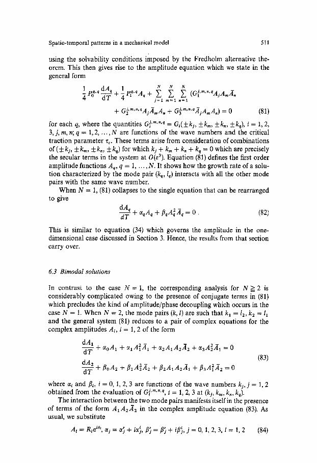
where r = ( / ~ 1 , / ~ 2 , 0 ) T and B the Jacobian matrix evaluated at R °, i = 1, 2, O °. We look for solutions of (100) of the form r = to exp(aT) and the solvability condition is [aI + B[ = 0. In this case, the analysis is straightforward and will be omitted. We show, by means of an example (see Table 1), the existence of stable solutions of type II and present numerical simulations of the amplitude equations for some parameter values (see Figs. 3 and 4).


Table 1. Table summarizing the linear stability for the amplitude equation for the case N = 2 for example (102). Here the linear analysis indicates two stable solutions of type II occurring when the steady state phase difference 20 0 ~ +__~/2 (see Fig. 5) and the other at 20 o ~ + rt/6.3. In this case all the single solution branches are unstable. Hence, small perturbations when the system indicates two-mode interaction will result in solutions of type II

cos(20 °) sin(20°)(R°)2xl0 -4 (R°)2xl0 -4 a(1, 2, 3) l(a, b) II

0.083 0.997 1.2 0.86 0.43, - 0.21, - 0.87 unstable unstable 0.083 - 0.997 2.9 2.2 - 0.5, - 0.6, - 2.7 unstable stable 0.879 0.478 0.98 0.83 0.02, - 0.02, - 0.64 unstable unstable 0.879 - 0.478 2.6 2.3 - 0.01, - 0.8, - 2.5 unstable stable

0.0250

0.0225

0.0200

0.0175

0.0156

0.0125

0.0100

o.oo75

0.0050

0.0025'

0.030

0.025

0.020

O. 015'

O.01d

0.005"

so' lo6 1so' 2od 256 306 s6 106 ls6 206 256 306

(b)

Fig. 3a, b. Numerical solution of the amplitude equations (81) for the parameter set (102) illustrating the case N - 2. a (i) and (ii) are, respectively, R1 and Rz as functions time. b (i), (ii) are the amplitude functions Re(Rz exp(i01)) and Re(R2 exp(i02)) plotted against time. Here, RI and R2 are of finite size and the observed solution is in a frequency locked oscillation in which the eigenfunetions corresponding to the two mode pairs (1, 2) and (2, 1) interact continuousIy


Fig. 4. Numerical calculation of the amplitude function for the case N = 2 from the numerical simulations of the full decomposed model plotted against time for the parameter set (102). The plots here agree closely with those of Fig. 3

We can calculate the l imiting value of the phase difference as follows: suppose tha t the ampl i tudes R~, j = 1, 2 ~ Ry as T ~ ~ . Then the limiting phase difference O will satisfy the equat ion

where

dO + Bo + Ao s in (20 + ~) = 0 (101)

d--~

tan(~) = - fl~(R°)2 - a~(R°)2 fl~(RO) 2 + ~ (RO) 2, B0 = (fl] - ~)2(R~)Z + (fit - ~])(R°) 2

Ao = {(fl~(R°) 2 - ~ ( n ° ) 2 ) 2 + (fl~(R°) 2 + ~(R°)2)2} 1/2,

This has a general solut ion of the form (96) and clearly shows the behaviour of O, the phase difference, for all times. When O is bounded for all times and non-osci l la tory, the result ing solutions represent a frequency locked oscilla- t ion in which the phase difference is constant.

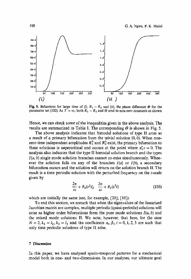
Example . The p a r a m e t e r set

/2 = 1.0, E = 5.0, D = 0.0125, s = 30.44, ~ = 0.025, r = 0.125 (102)

gives zc = 6.852 and the mode n u m b e r k~ = 5~ 2 which corresponds to the m o d e pairs (i , 2) and (2, 1). Hence the solutions characterized by these two m o d e pairs will interact. F o r e 2 = 0.0024, z = 6.8544. Evaluat ing the coefficients in the ampl i tude equat ions we have

a'oV = fl'oV = - 0.4640v, ~ v = fl'oV = 0, al = 36106.479 - 13259.248i,

a2 -- 3505.793 - 7615.846i, a3 = 2481.750 + 2939.747i,

fl~ = 16933.138 - 7912.699i, f12 = 4072.114 + 2042.421i,

f13 = 1 9 1 5 . 4 2 9 - 6 7 1 8 . 5 2 0 i ,

518 G. Ao Ngwa, P. K~ Maini

9E-4

8E-4'

~E-4

6E-4"

5E-4"

4E-4"

2~-4"

1E-4

1.4"

1.2'

1.0"

0.8"

0.6"

O. 4"

0,2

50' 100 15o' 200' 2s0' 300' ,...<

50' 106 ls0' 200" 250̀

(i) 300'

Fig. 5. Behaviour for large time of (i), R1 - R2 and (ii), the phase difference O for the parameter set (102). As T --* ~, both R1 - R2 and (9 tend to non-zero constants as shown

Hence, we can check some of the inequalities given in the above analysis. The results are summarized in Table 1. The corresponding (9 is shown in Fig. 5.

The above analysis indicates that bimodal solutions of type II arise as a result of a primary bifurcation from the trivial solution (0, 0). When non- zero time independent amplitudes R ° and R ° exist, the primary bifurcation to these solutions is supercritical and occurs at the point where ~ v = 0. The analysis also indicates that the type II bimodal solution branch and the types I(a, b) single mode solution branches cannot co-exist simultaneously. When- ever the solution falls on any of the branches l(a) or l(b), a secondary bifurcation occurs and the solution will return on the solution branch II. The result is a time periodic solution with the perturbed frequency on the t-scale given by

2re 2re + 01(~2t ) , - - + 02(~2t) (103)

o,) o )

which are initially the same (see, for example, 1-20], EIO]). To end this section, we remark that when the eigenvalues of the linearized

Jacobian matrix are complex, multiple periodic (quasi-periodic) solutions will arise as higher order bifurcations from the pure mode solutions I(a, b) and the mixed mode solutions II. We note, however, that here, for the case N = 2, k l = 12, kz = 11 and the coefficients ~, ]~, i = O, 1, 2, 3 are such that only time periodic solutions of type II arise.

7 Discussion

In this paper, we have analysed spatio-temporal patterns for a mechanical model both in one- and two-dimensions. In our analyses, our ultimate goal


has been to calculate the amplitude function that governs the spatio-temporal behaviour of the solutions for large time.

In the one-dimensional analysis, we have considered only cases where the uniform steady state is unstable to a solution with one mode number. The problem of bifurcations to solutions involving more that one mode number in the linear regime is a more complicated one and is still under investigation. In the one-dimensional case, we gave a detailed nonlinear analysis of the full nonlinear system and determined the leading order approximation to the amplitude function.

For the two-dimensional case, we presented an alternative reformulation of the two-dimensional model and justified it by showing that its underlying solutions agree with those of the original model. We explored the notion of mode degeneracy in the linear analysis of the system: that is, we considered the case where two or more mode pairs, associated with the same transverse wave number on a square domain, have the same growth rate in the linear regime. We further presented a detailed nonlinear analysis of spatio-temporal degenerate mode interaction. Our analysis has shown that, for the non-degenerate case, the behaviour of the system is a natural extension of the one-dimensional single mode solution. For the case where there are two degenerate mode pairs, a preliminary investigation showed that there are four possible time independent solutions for the amplitudes associated with each mode pair: the trivial solution, two single mode solutions (types I(a,) and I(b)) and a bimodal solution (type II). A further analysis showed that the only stable solution is the bimodal solution whereby the amplitude functions associated with each of the degenerate mode pairs are in a frequency locked oscillation. In this case, the solution of the full nonlinear system near the bifurcation point will be made up of some proportions of the eigenfunctions associated with those degenerate modes. This was verified by a numerical example. Although we only presented results for a single parameter set, we have considered several parameter sets and have verified in each case that the numerical solutions to the full model agree with the analytic solutions derived.

From our analysis on the simplified model, and for the parameter values we have used in the examples considered, we have not been able to locate any other stable solutions, aside from the bimodal solution of type II. We have no reason, however, to believe that in an analysis of spatio-temporal patterns in the full mechanochemical model, the situation will remain the same.

We remark that, to date, we do not know whether spatio-temporal patterns have any direct applications in the context in which the mechanochemical model was developed, namely embryonic development. However, the protrusive and regressive behaviour of cellular filopodia has been modelled as a spatio-tcmporal phenomenon (Lewis and Murray [9]). Moreover, spatio-temporal patterns abound in many biological and chemical systems. In this paper, we have shown how the mechanical model can be reduced by the Helmholtz decomposition to a much simpler sub-model and we have presented a framework for analysing spatio-temporal patterns and mode interactions within that system.

520 G.A. Ngwa, Po K. Maini

Acknowledgements. PKM would like to thank the Department of Applied Mathematics, University of Washington, Seattle and for support from the Robert F. Philip Endowment.

References

1. Bentil, D. E.: Dynamic Aspects of Pattern Formation in Embryology and Epidemi- ology. PhD thesis, Oxford University (1990)

2. Dautray, R. and Lions, J. -L.: Mathematical Analysis and Numerical Methods for Science and Technology, volume 2 & 3. Springer-Verlag (1988). Spectral Theory and Applications

3. Girault, V. and Raviart, P. -A.: Finite Element Approximation of the Navier-Stokes Equations, volume 749. Springer-Verlag, Berlin, Heidelberg, New York (1979). Lecture notes in Mathematics

4. Girault, Vo and Raviart, P. -A.: Finite Element Methods for Navier-Stokes Equations: Theory and algorithms, volume 5. Springer-Verlag, Berlin, Heidelberg, New York (1986). Springer Series in Computational Mathematics

5. Grindrod, P.: Patterns and Waves: The Theory and Applications of Reaction-Diffusion Equations. Clarendon Press, Oxford (1991). Oxford Applied Mathematics and Com- puting Science Series

6. Harris, A. K., Stopak, D. and Wild, D.: Fibroblast traction as a mechanism for collagen morphogenesis. Nature 290, 249-251 (1981)

7. Harris~ A. K., Ward, P. and Stopak, D.: Silicone rubber substrate; a new wrinkle in study of cell locomotion. Science. 208, 177-179 (1980)

8. Hassard, B. D., Kazarinoff, N. D. and Wan, Y. -H.: Theory and Application of Hopf Bifurcation, volume 41. Cambridge University Press (1981). Lond. Math. Soc. Lecture Notes

9. Lewis, M. A. and Murray, J. D.: Analysis of dynamic and stationary pattern formation in the cell cortex. J. Math. Biol. 31, 25-71 (1992)

10. Magolis, S. B. and Matkowsky, B. J.: New modes of quasi periodic combustion near a degenerate hopf bifurcation point. SIAM J. Appl. Math. 48, 828-853 (1988)

11. Maini, P. K. and Murray, J. D.: A nonlinear analysis of a mechanochemical model for biological pattern formation. SIAM J. Appl. Math. 48, 1064-1072 (1988)

12. Margolis, S. B.: New routes to quasi-periodic combustions of solids and high-density fluids near resonant hopf bifurcation points. SIAM J. Appl. Math. 51, 693-726 (1991)

13. Morton, K. W. and Baines, M. J.: Numerical Methods for Fluid Dynamics III, volume 17. Clarendon Press, Oxford (1988). The Institute of Mathematics and its Applications Conference Series

14. Murray, J. D. and Oster, G. F.: Mechanical aspects of mesenchymal morphogenesis. J. Embryol. Morph. 78, 83-125 (1985)

15. Murray, J° D.: Mathematical Biology. Springer Verlag, Berlin, Heidelberg (1989) 16. Ngwa, G. A.: The Analysis of Spatial and Spatio-temporal Patterns in Models for

Morphogenesis. PhD thesis, Oxford University (1993) 17. Ochoa, F. L. and Murray, J. D.: A nonlinear analysis for spatial structure in a reaction

diffusion model. Bull. Math. Biol. 45(6), 917-930 (1983) 18. Oster, G. F., Murray, J. D. and Maini, P. K,: A model for chondrogenic condensations

in the developing limb; the role of extracellular matrix and cell tractions. J. Embryol. Morph. 89, 93-112 (1985)

19. Perelson, A. S., Maini, P. K., Murray, J. D., Hyman, J. M. and Oster, G. F.: Nonlinear pattern selection in a mechanochemical model for morphogenesis. J. Math. Biol. 24, 525-541 (1986)

20. Steen, P. H. and Davis, S. H.: Quasi periodic oscillations near a point of strong resonance. SIAM J. Appl. Math. 42, 1345-1368 (1982)

spatio-temporal patterns in a mechanical model for ... publications/50.pdf · spatio-temporal...

Documents