adaptive scheduling for operating room management
TRANSCRIPT

University of Kentucky University of Kentucky
UKnowledge UKnowledge
Theses and Dissertations--Mechanical Engineering Mechanical Engineering
2017
ADAPTIVE SCHEDULING FOR OPERATING ROOM MANAGEMENT ADAPTIVE SCHEDULING FOR OPERATING ROOM MANAGEMENT
Honghan Ye University of Kentucky, [email protected] Author ORCID Identifier:
http://orcid.org/0000-0001-5329-7344 Digital Object Identifier: https://doi.org/10.13023/ETD.2017.095
Right click to open a feedback form in a new tab to let us know how this document benefits you. Right click to open a feedback form in a new tab to let us know how this document benefits you.
Recommended Citation Recommended Citation Ye, Honghan, "ADAPTIVE SCHEDULING FOR OPERATING ROOM MANAGEMENT" (2017). Theses and Dissertations--Mechanical Engineering. 88. https://uknowledge.uky.edu/me_etds/88
This Master's Thesis is brought to you for free and open access by the Mechanical Engineering at UKnowledge. It has been accepted for inclusion in Theses and Dissertations--Mechanical Engineering by an authorized administrator of UKnowledge. For more information, please contact [email protected].

STUDENT AGREEMENT: STUDENT AGREEMENT:
I represent that my thesis or dissertation and abstract are my original work. Proper attribution
has been given to all outside sources. I understand that I am solely responsible for obtaining
any needed copyright permissions. I have obtained needed written permission statement(s)
from the owner(s) of each third-party copyrighted matter to be included in my work, allowing
electronic distribution (if such use is not permitted by the fair use doctrine) which will be
submitted to UKnowledge as Additional File.
I hereby grant to The University of Kentucky and its agents the irrevocable, non-exclusive, and
royalty-free license to archive and make accessible my work in whole or in part in all forms of
media, now or hereafter known. I agree that the document mentioned above may be made
available immediately for worldwide access unless an embargo applies.
I retain all other ownership rights to the copyright of my work. I also retain the right to use in
future works (such as articles or books) all or part of my work. I understand that I am free to
register the copyright to my work.
REVIEW, APPROVAL AND ACCEPTANCE REVIEW, APPROVAL AND ACCEPTANCE
The document mentioned above has been reviewed and accepted by the student’s advisor, on
behalf of the advisory committee, and by the Director of Graduate Studies (DGS), on behalf of
the program; we verify that this is the final, approved version of the student’s thesis including all
changes required by the advisory committee. The undersigned agree to abide by the statements
above.
Honghan Ye, Student
Dr. Wei Li, Major Professor
Dr. Haluk E. Karaca, Director of Graduate Studies

ADAPTIVE SCHEDULING FOR OPERATING ROOM MANAGEMENT
_________________________________
THESIS _________________________________
A thesis submitted in partial fulfillment of the
requirement for the degree of Master of Science in Mechanical Engineering in the College of Engineering at the University of Kentucky
By
Honghan Ye
Lexington, Kentucky
Co-Directors: Dr. Wei Li, Assistant Professor of Mechanical Engineering
and Dr. Fazleena Badurdeen, Associate Professor of Mechanical Engineering
Lexington, Kentucky
2017
Copyright© Honghan Ye 2017

ABSTRACT OF THESIS
ADAPTIVE SCHEDULING FOR OPERATING ROOM MANAGEMENT The perioperative process in hospitals can be modelled as a 3-stage no-wait flow shop. The utilization of OR units and the average waiting time of patients are related to makespan and total completion time, respectively. However, minimizations of makespan and total completion time are NP-hard and NP-complete. Consequently, achieving good effectiveness and efficiency is a challenge in no-wait flow shop scheduling. The average idle time (AIT) and current and future idle time (CFI) heuristics are proposed to minimize makespan and total completion time, respectively. To improve effectiveness, current idle times and future idle times are taken into consideration and the insertion and neighborhood exchanging techniques are used. To improve efficiency, an objective increment method is introduced and the number of iterations is determined to reduce the computation times. Compared with three best-known heuristics for each objective, AIT and CFI heuristics can achieve greater effectiveness in the same computational complexity based on a variety of benchmarks. Furthermore, AIT and CFI heuristics perform better on trade-off balancing compared with other two best-known heuristics. Moreover, using the CFI heuristic for operating room (OR) scheduling, the average patient flow times are decreased by 11.2% over historical ones at University of Kentucky Health Care. KEYWORDS: Operating Room Scheduling, No-wait Flow Shop, Makespan and Total Completion Time, Trade-off Balancing, Heuristics.
Honghan Ye Student’s Signature
04/07/2017 Date

ADAPTIVE SCHEDULING FOR OPERATING ROOM MANAGEMENT
By
Honghan Ye
Dr. Wei Li Co-Director of Thesis
Dr. Fazleena Badurdeen Co-Director of Thesis
Dr. Haluk E. Karaca Director of Graduate Studies
04/18/2017 Date

iii
ACKNOWLEDGMENTS
First of all, I want to thank Dr. Wei (Mike) Li for taking me on as his student. His
critical thinking for doing research inspires me to construct my own research topic. In
addition, Dr. Li provided timely and instructive comments and help at every stage of the
thesis process, allowing me to finish this program on time.
Next, I want to thank Dr. Jawahir and Dr. Badurdeen for agreeing to be a part of
my committee. Each individual provided a wealth of insight that guided and challenged
my thinking in and out of class. I am truly grateful to Dr. Miao at HFUT for helping me to
start in this research field in my undergraduate study.
In addition to the technical and academic assistance above, I want to thank my
parents for always encouraging me so that I can go through all the ups and downs. I thank
my friends for taking the time with me to offer their friendship and laughter. I thank my
lab mate Amin for his kind help in my research and life. Finally, I want to thank my
roommates for their care and support.

iv
TABLE OF CONTENTS
Acknowledgments ............................................................................................................. iii
List of Tables .................................................................................................................... vi
List of Figures .................................................................................................................. vii
Chapter One: Introduction
1.1 Background ........................................................................................................1
1.2 Motivation ..........................................................................................................2
1.3 The challenges in no-wait flow shop scheduling ...............................................5
1.4 The contribution .................................................................................................8
1.5 The structure of this thesis .................................................................................9
Chapter Two: Literature review
2.1 Heuristics for no-wait flow shop to minimize Cmax and ∑Cj ...........................11
2.1.1 Heuristics for no-wait flow shop to minimize Cmax .........................12
2.1.2 Heuristics for no-wait flow shop to minimize ∑Cj ..........................14
2.2 Heuristics for multi-objective optimization in no-wait flow shop ...................17
2.3 Statistical process control in operating room scheduling ................................19
Chapter Three: Methodology
3.1 Problem description .........................................................................................22
3.2 Initial Sequence Algorithm (ISA) ....................................................................25
3.3 AIT heuristic to min(Cmax) ...............................................................................27
3.4 CFI heuristic to min(ƩCj) .................................................................................30
3.5 Objective increment method to calculate total completion time (TCT) .........35
Chapter Four: Case study
4.1 Schemes to carry out case studies ....................................................................38
4.2 Results of case study on Fm |nwt| Cmax problems .............................................41
4.2.1 Small-scale instances .......................................................................41
4.2.2 Large-scale instances .......................................................................43
4.3 Results of case study on Fm |nwt| ∑Cj problems ..............................................46
v
4.3.1 Small-scale instances .......................................................................46
4.3.2 Large-scale instances .......................................................................48
4.4 Trade-off balancing ..........................................................................................53
4.5 Case study on UKHC historical data ...............................................................56
Chapter Five: Conclusion and future work
5.1 Concluding remarks .........................................................................................62
5.2 Future work ......................................................................................................64
References ..........................................................................................................................67
Vita .....................................................................................................................................77

vi
LIST OF TABLES
Table 2.1: The summary of heuristics to minimize Cmax ..................................................12
Table 2.2: The summary of heuristics to minimize ∑Cj ....................................................15
Table 3.1: Processing times of a 6-job 5-machine instance ..............................................27
Table 3.2: Distance matrix for an example to min(Cmax) ...................................................30
Table 3.3: Processing times of a 5-job 4-machine instance. ..............................................33
Table 3.4: Distance matrix for an example to min(ƩCj) ....................................................34
Table 4.1: Average Relative and Maximum percent deviations (ARPD & MPD) for small-
scale instances to min(Cmax) (%) ........................................................................................42
Table 4.2: Average Relative and Maximum percent deviations (ARPD & MPD) for large-
scale instances to min(Cmax) (%) ........................................................................................43
Table 4.3: ANOVA results to min(Cmax) (95% Confidence Interval) ...............................45
Table 4.4: Paired t-tests results to min(Cmax) (α=0.05) .....................................................46
Table 4.5: Average Relative and Maximum percent deviations (ARPD & MPD) for small-
scale instances to min(∑Cj) (%) .........................................................................................47
Table 4.6: Average Relative and Maximum percent deviations (ARPD & MPD) for large-
scale instances to min(∑Cj) (%) ........................................................................................49
Table 4.7: ANOVA results to min(∑Cj) (95% Confidence Interval) ...............................51
Table 4.8: Paired t-tests results to min(∑Cj) (α=0.05) ......................................................51
Table 4.9: CPU times of four heuristics for large-scale instances to min(∑Cj) .................53
Table 4.10: APFT (minutes) and standard deviation for four heuristics and UKHC .......57

vii
LIST OF FIGURES
Figure 1.1: The perioperative process .................................................................................3
Figure 1.2: Decision making problems and complexity .....................................................6
Figure 2.1: The control chart of effective service rate of surgery type 1 (S1) ...................20
Figure 3.1: Distance between two adjacent jobs ................................................................23
Figure 4.1: Deviations of Cmax as the number of jobs or machines increases ....................44
Figure 4.2: Deviations of TCT as the number of jobs or machines increases ....................50
Figure 4.3: The deviation from upper bound with the value of r ......................................52
Figure 4.4: The performances of each heuristic given different values of α .....................56
Figure 4.5: Capability analysis of average patient flow times in 250 days .......................59
Figure 4.6: X-bar&R charts of average patient flow times ................................................60
1
Chapter 1 Introduction
1.1 Background
Operating rooms (OR) are the most cost and revenue intensive areas in hospitals.
In 2002, there were 36.5 million hospital stays in the United States, with an average length
of stay of 4.5 days and an average cost of $10,400 per stay. About 21.8% of hospital stays
in 2012 were surgical (Weiss and Elixhauser, 2014). In surgical procedures, ORs have been
estimated to account for over 40% of total expenditure of a hospital (Denton et al., 2007).
On the one hand, the operating rooms are one of most important resources, which has the
largest cost and revenues (Ghazalbash et al, 2012). Mean hospital costs of surgical stays
are $21,200 in 2012, which is 2.5 times the mean costs of $8,500 for medical stays and
nearly 5 times the mean costs of $4,300 for maternal and neonatal stays (Moore et.al, 2014).
On the other hand, because of the aging population, there is a sharply increasing trend of
demand for surgical services in recent years (Etzioni et al., 2003). There were around 51
million inpatient surgical procedures performed in the United States in 2010, according to
the latest data from the Centers for Disease Control and Prevention (Hall and Owings,
2014).
Long waiting time, a large number of emergencies, and resource overload are
coming along with this increasingly demand in healthcare systems (Meskens et.al 2013).
Therefore, hospital managers are continuously looking for new methods to increase the
utilization of OR units and to reduce the average waiting time of patients (Cardoen et al.,
2010). From flow shop perspective, the utilization of an OR unit is defined as the workload
divided by the completion time of the last patient, where workload is the sum of case times.
The average waiting time is defined as the length of time that a patient stays in the

2
perioperative (periop) process, which consists of the preoperative (preop), intraoperative
(intraop), and postoperative (postop) stages. Average waiting time can be represented by
the average flow time in a flow shop, which is the total completion time divided by the
number of patients. Minimization of maximum completion time or makespan can improve
OR utilization, which directly reduces surgical overtime and its cost. Minimization of
average waiting time can improve patient flow through the periop process, which improves
patient throughput and generates more revenue.
1.2 Motivation
OR scheduling is extraordinarily complicated. The scheduling process must take
different surgical specialties into consideration, each of which has different priorities,
procedures, and case times. It also should consider different resources for specialties and
surgical procedures. Resources include human resources (e.g., surgeons, anesthesiologists,
nurses, and staff), equipment used in different periop stages (e.g., induction equipment,
surgical instruments, and electro-medical equipment). In addition, the scheduling process
must take into account the disturbances across the periop process, such as emergency cases,
cancellations, or no-shows, variations in case times due to surgical complexities, post-
anesthesia care units (PACU) boarding, and length of stay in the periop process (Bosse et
al., 2013). Another consideration is about different preferences of stakeholders involved in
scheduling processes (Glouberman and Mintzberg, 2001), which might possibly be in
conflict.
Typically, the three stages of the periop process are shown in Figure 1.1 (Gupta,
2007). There are many operations in each stage. For example, the collection of patient
information and the preparation for surgeries occur in the preop stage, surgeries occur in

3
ORs in the intraop stage, and PACU, intensive care units (ICU), or ward for recovery are
in the postop stage. Each stage requires different resources to accommodate specific patient
needs. For simplicity, we model the OR scheduling problem across the periop process as a
3-stage no-wait flow shop.
Figure 1.3: The perioperative process
The three stages in the periop process are tightly coupled, because performance of
one stage affects the performance of adjacent stages. This is also the characteristic of a 3-
stage no-wait flow shop. For example, the delay of patients from a preop unit to ORs lowers
OR utilization, especially for the first case (Roberts et al., 2015), which is the performance
of stage 1 affects that of stage 2. Marcon and Dexter (2006) studied the impact of OR
performance on PACU staffing, and found the performance of stage 2 affects that of stage
3. These two examples show how upstream stages affect downstream stages. Downstream
stages can affect upstream stages as well. For example, when all postop beds are occupied,
blocking occurs between the intraop and postop stages. Consequently, case times are
extended because patients cannot be transferred out of ORs in the absence of recovery beds
in PACU or ICU (Augusto et al., 2010; Wang et al., 2015). This scenario is accentuated
with PACU boarding, which means patients stay in PACU overnight (Price et al., 2011).
Therefore, the 3-stage no-wait flow shop is suitable to model the periop process, in which
no waiting time between stages is allowed.
Preoperative Intraoperative Postoperative

4
To evaluate OR scheduling across the periop process, there are two main
performance measures: OR utilizations and average waiting time. From flow shop
perspective, Cmax,2 as the maximum completion time of the intraop stage affects OR
utilization, because utilization equals to the workload divided by the working period, and
the working period is equal to the completion time of the last job (Cmax,2) minus the start
time of the first job. 𝐶𝐶̅=∑Cj,3/n as the average completion time of the postop stage affects
average waiting time, which is the total completion time in the postop stage (∑Cj,3) divided
by the number of patients (n) (Pinedo, 2014). There are several other objectives to evaluate
the performance of the periop process. The objective of throughput is closely related to the
average patient waiting time. According to the Little’s Law, the average inventory in a
system equals the average cycle time (which includes waiting time and processing time)
times the average throughput (Little, 1961). The objective of leveling resources is mainly
to develop a schedule by smoothing resource occupancies without over usage. Leveling
resources involves the utilization and average flow time in each of the three stages across
the periop process. Therefore, maximum completion time and average completion time are
most important performance measures, which define the utilizations and average waiting
times.
ORs are the largest cost center and the greatest revenue source simultaneously for
hospitals (Ghazalbash et al, 2012). OR scheduling affects the progression of surgical cases
going through the periop process. Most hospitals use a three-phase block scheduling
framework to plan this progression. OR planning is phase 1, focusing on long-term
strategies, where resources and services are allocated to OR blocks. OR scheduling is phase
2, focusing on medium-term tactics, where a master surgical schedule (MSS) is generated.

5
The MSS generates the number of available surgical suites, operation hours, and OR block
times for a type of services. Case sequencing is phase 3, focusing on short-term execution
of MSS, where daily surgical cases are sequenced by operating rooms (Banditori et al.,
2013, Cardoen et al., 2010).
Different sequencing methods can address stakeholders’ objectives differently. For
example, the longest processing time (LPT) rule is recommended to improve OR utilization
(Magerlein and Martin, 1978; Gupta and Denton, 2008). The shortest processing time (SPT)
rule is recommended to reduce the number of case delays and to speed up patient flows
across the periop process (Testi et al., 2007). Both approaches give rise to schedule slippage
in that we cannot generate the best solutions of OR utilization and patient time
simultaneously through LPT and SPT rules. Therefore, it’s of great interest and importance
to balance different performance measures and to achieve adaptive scheduling and control.
1.3 The challenges in no-wait flow shop scheduling
Given the above complexities in OR scheduling across the periop process, we
model it as min(Cmax and ∑Cj) problems for a 3-machine no-wait flow shop. Therefore, we
have the following challenges in no-wait flow shop scheduling.
For the convenience of describing scheduling problems in no-wait flow shop, we
use Fm |nwt| Cmax to denote minimization of makespan and Fm |nwt| ∑Cj to denote
minimization of total completion time, where Fm is for a flow shop problem with m
machines, nwt for the constraint of no-wait, and Cmax for the objective to minimize
maximum completion time and ∑Cj for the objective of minimize total completion time
(Graham et al., 1979).

6
No-wait flow shop scheduling problems are categorized as combinatorial
optimization problems in which the feasible region is countable (Garey and Johnson, 2002).
The complexity of different classes of problems in combinational optimization is shown in
Figure 1.2. Fm |nwt| Cmax problems have been proved to be NP-hard when the number of
machines is larger than or equal to three, and Fm |nwt| ∑Cj problems are NP-complete when
the number of machines is larger than or equal to two (Garey and Johnson, 2002; Röck,
1984). For an NP-complete or NP-hard problem, we cannot describe the problem by
polynomials completely, or in other words, we cannot optimally solve the problem in a
polynomial time. As a result of the NP-hardness or NP-completeness, it is extremely time
consuming to find optimal solutions by using exact methods even for moderate-scale
problems (Ding et al., 2014). Consequently, the complexity of these problems makes it
difficult to optimally improve OR utilization and/or reduce average waiting time, although
optimal solutions can be derived for 2-machine flow shop production to minimize Cmax
(Johnson, 1954), and for 1-machine production to minimize ∑Cj. (Pinedo, 2014).
Figure 1.4: Decision making problems and complexity (Samarghandi, 2011)

7
Given 𝐶𝐶̅=∑Cj/n, we can see that the completion time of the last job n (Cmax) is
included in ∑Cj. If n is fixed, minimization of total completion time, min(∑Cj), is the same
as min(𝐶𝐶̅ ). However, min(Cmax) does not necessarily mean min(∑Cj), or vice versa,
although Cmax is included in ∑Cj. These two scheduling objectives are inconsistent. In the
investigation of OR scheduling methods (Li et al., 2014), the authors found these two
common OR scheduling objectives were inconsistent. One objective of min(Cmax) is to
minimize the maximum completion time for the last surgical case of the day. The second
scheduling objective of min (∑Cj) is to minimize the total completion time of an OR’s daily
slate, which is analogous to minimizing the average completion time if the number of
surgeries (n) is fixed, i.e., to min (𝐶𝐶̅), where j = 1,…,n. This inconsistency partially explains
why delays can occur between any two perioperative stages -- improving utilization in any
stage may reduce patient flow out of that stage, i.e., minimizing Cmax may maximize ∑Cj.
Consequently, such inconsistency between min(Cmax) and min (∑Cj) makes it more
difficult to improve OR utilization and reduce average waiting time at the same time, which
is a multi-objective optimization problem.
As OR management concerns evolve, on the one hand, the system changes over
time and the relationship among system components creates inconsistencies in system
performance (Davis et al., 2013; Beck et al., 2014; Pellegrino, 2015). Therefore, an OR
scheduling process must adapt to changing relationships and facilitate OR management as
concerns evolve. On the other hand, OR schedules are constructed as static timetables, with
little ability to adapt to dynamic changes in demand (e.g., emergency cases or case time
variation). With the time goes by, OR planning, scheduling, and control are interacted with
each other. For example, if the performance at this time is not good as expected, it may

8
affect the schedulers to adjust scheduling at next time, or even affect the OR manager to
change resource allocation at the next planning time. Consequently, the complexity of the
interaction between OR planning, scheduling, and control makes it difficult to achieve
adaptive scheduling in perioperative process.
1.4 The contribution
The contribution of our work comes from three aspects: (1) new methods to
min(Cmax) and min(∑Cj) for no-wait flow shop respectively; (2) a trade-off balancing
function to evaluate trade-off between Cmax and ∑Cj; (3) a validation of the CFI heuristic
based on the historical data at University of Kentucky HealthCare (UKHC), along the time
horizon.
First, we propose an initial sequence algorithm (ISA), based on which we propose
an average idle time (AIT) heuristic to min(Cmax), and a current and future idle time (CFI)
heuristic to min(∑Cj) for no-wait flow shop scheduling. In the ISA, we treat current idle
time and future idle time differently by a lever concept introduced in Li et al (2011).
Consequently, in the initial sequence, we assign higher weights to current idle times
generated by jobs in the head of a sequence than those generated by jobs in the tail of the
sequence. In both AIT and CFI heuristics, search techniques of insertion and neighborhood
exchanging are used to further improve the solutions generated by the ISA. Based on a
variety of benchmarks and randomly generated instances, our AIT and CFI heuristics
perform better than other best-known existing heuristics for no-wait flow shop scheduling.
Second, we introduce a trade-off balancing (TOB) function for no-wait flow shop
scheduling to evaluate trade-off between Cmax and ∑Cj. In the evaluation scheme, we assign

9
different preferences to each objective. The results show that the proposed heuristics
perform better than the LS (Laha and Sapkal, 2014) and CH (Li et al., 2008) heuristics.
Third, we use statistical process control (SPC) and control charts to validate our
CFI heuristic for operating room (OR) scheduling across the periop process in a healthcare
system. The results indicate that potentially 3,000 additional patients could be served in a
year if our CFI heuristic was applied for sequencing.
1.5 The structure of this thesis
The rest of the thesis is organized as follows:
The chapter 2 provides a thorough literature review, including current status of
heuristics to minimize the Cmax and ∑Cj, current status of multi-objective optimizations in
no-wait flow shop scheduling, and statistical process control in OR scheduling.
The chapter 3 gives the methodology of the proposed heuristics. The problem
description of no-wait flow shop is provided first. Then the initial sequence algorithm (ISA)
is proposed to generate the initial sequence. Based on ISA, the AIT and CFI heuristics are
given in detail to minimize Cmax and ∑Cj, respectively. The increment objective method is
introduced to reduce the computational complexity from O(n) to O(1) when using
neighborhood exchanging technique to calculate the total completion time.
The chapter 4 provides the results of case study. First, the performance of AIT and
CFI heuristics will be compared with other existing heuristics based on a variety of
benchmarks and generated data. Second, by using trade-off balancing (TOB) function,
based on the Taillard’s benchmarks, the performances of the trade-off between Cmax and
∑Cj for each heuristic are compared. Last, based upon the historical data at the University
of Kentucky HealthCare, the SPC charts with the CFI heuristic and UKHC are presented.

10
The chapter 5 presents the conclusions and directions for future research.

11
Chapter 2 Literature review
This chapter focuses on the literature review on three topics. First, heuristics
currently for single objective optimization of no-wait flow shop scheduling are introduced,
which are to minimize maximum completion time (Cmax) and total completion time (∑Cj),
respectively. Second, heuristics currently for multi-objective optimizations of no-wait flow
shop scheduling are presented. Finally, statistical process control (SPC) methods are
introduced for operating room scheduling.
2.1 Heuristics for no-wait flow shop to minimize Cmax and ∑Cj
Minimizations of Cmax and ∑Cj are NP-hard and NP-complete problems for no-wait
flow shop production, and it is extremely time consuming to find optimal solutions using
exact methods for such problems. There are mainly two ways to find near-optimal solutions
by using heuristics and meta-heuristics (Ruiz and Maroto, 2005). The heuristics can be
grouped into constructive heuristic and improvement heuristics. The constructive heuristics
build a feasible schedule from scratch, such as the NEH heuristic (Nawaz et al., 1983),
while the improvement heuristics improve the performance of feasible schedules by
applying some search techniques, such as neighborhood exchanging (Dannenbring, 1997).
Meta-heuristics start from an initial schedule constructed by constructive or improvement
heuristics, and generate better performance by iterations until a stopping criterion is
satisfied, such as the computation time, the number of iterations, etc. Typical examples of
meta-heuristics are simulated annealing (Ogbu and Smith, 1990), tabu search (Moccellin,
1995), genetic algorithms (Murata et al., 1996). Compared to heuristics, meta-heuristics
can generate better results in general, but have much higher computational complexities

12
and take much longer computation time to solve even for moderately scaled instances.
Consequently, with such a high computation burden, meta-heuristics are not commonly
applied in industry where problem scales are changing from moderate to large. Therefore,
heuristics with small computational efforts are proposed to minimize Cmax and ∑Cj
respectively in the thesis for adaptive scheduling.
2.1.1 Heuristics for no-wait flow shop to minimize Cmax
Table 2.1 shows a summary of the heuristics for the Fm |nwt| Cmax problems
reviewed in a chronological order.
Table 2.1: The summary of heuristics to minimize Cmax Year Author(s) Acronym Comments
1976 Bonney and Gundry BG Based on a slope index
1980 King and Spachis KS Minimum covering level
1993 Gangadharan and
Rajendran GR
The jobs with increasing trends in
processing time are processed ahead
1994 Rajendran RAJ Adjacent jobs match and put last job
with short processing time
2008 Framinan and Nagano FN Based on Farthest Insertion
Travelling Salesman Procedure
2008 Li et al. CH Based on job insertion and
interchange techniques
2009 Laha and Chakraborty LC Based on job insertion considering
two consecutive jobs as a block
2016 Ye et al. ADT Based on average departure time
Bonney and Gundry (1976) and King and Spachis (1980) pioneered constructive
heuristics for solving Fm |nwt| Cmax problems. Bonney and Gundry (1976) proposed a slope

13
index method to sequence jobs. King and Spachis (1980) proposed a minimum covering
level (MCL) method for solving Fm |nwt| Cmax problems.
Gangadharan and Rajendran (1993) and Rajendran (1994) proposed two heuristics,
named GR and RAJ, to solve the same problem. GR heuristic first sequences jobs in an
increasing or decreasing trend of their times, then uses an insertion technique to improve
the performance of the initial sequence. RAJ heuristic makes the adjacent jobs “match”,
similar to the GR heuristic based on the increasing or decreasing trend of a job, as much as
possible in order to minimize the inter-job delays and has the last job with short processing
time. The computational results showed that GR and RAJ heuristics were superior to the
heuristics proposed by BG heuristic (Bonney and Gundry, 1976) and KS heuristic (King
and Spachis, 1980).
Framinan and Nagano (2008) proposed a new heuristic based on Farthest Insertion
Travelling Salesman Procedure (FITSP) (Syslo, 1983), and compared this new heuristic
with random ordering, descending sum of processing times, and RAJ initial sequence
(Rajendran, 1994). The experimental results showed that the new heuristic performed
better than other three heuristics.
Based on the objective increment method, Li et al. (2008) proposed a composite
heuristic (CH) using job insertion and exchange techniques, and experimental results
showed that the CH heuristic performed better than the GR (Gangadharan and Rajendran,
1993) and RAJ (Rajendran, 1994) heuristics and used the least CPU time for the same
instances.
Laha and Chakraborty (2009) proposed a constructive heuristic (LC) to solve Fm
|nwt| Cmax problems. The principle of job insertion in the LC heuristic is that every two

14
consecutive jobs are selected as a block from the initial sequence, which is to be inserted
into a partial sequence, and each job in the block is inserted into each possible position of
the partial sequence. Through each insertion, choose the best partial sequence with the
smallest makespan and update the partial sequence until all jobs from the initial sequence
have been inserted into the partial sequence. The computational results showed that the LC
heuristic was significantly better than the GR (Gangadharan and Rajendran, 1993), RAJ
(Rajendran, 1994) heuristics.
Ye et al. (2016) proposed an average departure time (ADT) heuristic to minimize
Cmax for no-wait flow shop production. They first proposed the initial sequence based on
the average of idle times, and then use group and insertion techniques to improve the initial
solutions. The computational results showed that the ADT heuristic performed better than
GR (Gangadharan and Rajendran, 1993), RAJ (Rajendran, 1994), and modified NEH
(Nawaz et al., 1983) heuristics.
Overall, many researchers adopt the insertion and exchange techniques to improve
the initial solutions for solving Fm |nwt| Cmax problems. However, the properties of no-wait
flow shop scheduling still needs investigation to generate more effective and efficiency
heuristics.
2.1.2 Heuristics for no-wait flow shop to minimize ∑Cj
Table 2.2 shows a summary of the heuristics for the Fm |nwt| ∑Cj problems reviewed
in a chronological order.

15
Table 2.2: The summary of heuristics to minimize ∑Cj Year Author(s) Acronym Comments
1990 Rajendran and
Chaudhuri
RC Based on preference relations
2000 Bertolissi BER Temporary flow time
2004 Aldowaisan and
Allahverdi
PH1(p) NEH insertion scheme and pair-wise
exchange
2010 Framinan et al. FNM Insertion and exchange neighborhood
techniques
2013 Gao et al. IB Improved Bertolissi heuristic
2013 Sapkal and Laha SL Priority on the bottleneck
2014 Laha et al. PSI Penalty-shift-insertion scheme
2014 Laha and Sapkal LS Based on average departure time
Rajendran and Chaudhuri (1990) proposed an RC heuristic based on the preference
relations for the Fm |nwt| ∑Cj problems. According to the results of computational
experiments, their RC heuristic was more effective on the Fm |nwt| ∑Cj problems than BG
heuristic (Bonney and Gundry, 1976) and KS heuristic (King and Spachis, 1980).
Bertolissi (2000) proposed a BER heuristic to min (∑Cj) based on an initial
sequence and job insertion technique. The initial sequence is generated by comparing
temporary flow times of each pair of jobs. Job insertion technique is applied to improve
the performance by the initial sequence. The computational results showed that the BER
heuristic performed better than RC heuristic (Rajendran and Chaudhuri, 1990) and BG
heuristic (Bonney and Gundry, 1976).
Aldowaisan and Allahverdi (2004) proposed six improved heuristics by using three
different search methods, first by the same insertion scheme as in the NEH heuristic
(Nawaz et al., 1983), second by the same insertion technique as in Rajendran and Ziegler

16
(1997), and third by the adjacent pair-wise neighborhood exchanging method. The NEH
heuristic is considered to be the best constructive heuristic to minimize makespan for
permutation flow shop production (Kalczynski and Kamburowski, 2007). Among the six
improved heuristics, the PH1(p) heuristic performed significantly better than the heuristic
proposed by RC heuristic (Rajendran and Chaudhuri, 1990) and the genetic algorithm
proposed by Chen et al (1996).
Framinan et al. (2010) proposed an FNM constructive heuristic to minimize total
completion time based on insertion and exchange neighborhood techniques. The results of
their case studies showed that the FNM heuristic performed better than the RC heuristic
proposed by Rajendran and Chaudhuri (1990), the PH1(p) heuristic by Aldowaisan and
Allahverdi (2004), BER heuristic by Bertolissi (2000), and the heuristic by Fink and Voß
(2003).
Using the constructive procedure as in Laha and Chakraborty (2009), Gao et al.
(2013) proposed two constructive heuristics, the improved standard deviation (ISD)
heuristic and the improved Bertolissi (IB) heuristic, which were developed from the
standard deviation heuristic by Gao et al. (2011) and the BER heuristic (Bertolissi, 2000),
respectively. The results of their case studies showed that the IB heuristic performed better
than the NEH (Nawaz et al., 1983) and BER heuristic (Bertolissi, 2000).
Sapkal and Laha (2013) proposed an efficient heuristic (SL heuristic) to minimize
total flow time. The initial sequence is generated based on the assumption that the priority
of a job in the initial sequence is given by the sum of processing times on the bottleneck
machine. An insertion technique, the same as that in LC heuristic proposed by Laha and
Chakraborty (2009), is applied to improve the performance of the initial sequence. The

17
results showed that the SL heuristic performed better than RC heuristic (Rajendran and
Chaudhuri, 1990) and BER heuristic (Bertolissi, 2000).
Laha et al. (2014) proposed a penalty-shift-insertion (PSI) heuristic for Fm |nwt| ∑Cj
problems, and their computational experiments showed that the PSI heuristic was relatively
more effective and efficient than other heuristics in the literature at the time.
Recently, Laha and Sapkal (2014) proposed an improved LS heuristic, and results
showed that the LS heuristic performed better than the PH1(p) heuristic (Aldowaisan and
Allahverdi, 2004) and the FNM heuristic (Framinan et al., 2010).
2.2 Heuristics for multi-objective optimization in no-wait flow shop
Although in the past decades, efforts have been made to obtain high-quality
solutions with acceptable computation times by optimizing a single objective, multi-
objective optimization is more reasonable for flow shop production scheduling in reality,
because some objectives are inconsistent, such as min(Cmax) and min(ƩCj) as indicated in
Li et al., (2014). Allahverdi and Aldowaisan (2002) proposed a PAAH heuristic to
minimize a weighted sum of makespan and total completion time based on insertion and
exchange techniques. By their computational results, the PAAH heuristic performed better
than existing heuristics for the single objective of Cmax and ∑Cj, such as RC heuristic
(Rajendran and Chaudhuri, 1990), GR (Gangadharan and Rajendran, 1993), RAJ
(Rajendran, 1994), and a genetic local search algorithm for multi-objective in flow shop
(Ishibuchi and Murata, 1998).
Liao et al. (2008) proposed an evolutionary algorithm and Liu et.al (2008) proposed
a new hybrid genetic algorithm. Both methods are for no-wait flow shop production to
minimize both makespan and total flow time. A non-dominated sorting strategy and an

18
objective increment strategy are integrated into these two methods. Their experimental
results showed that the proposed methods outperformed the PAAH heuristic (Allahverdi
and Aldowaisan, 2002) and other heuristics.
There are several other multi-objectives for no-wait flow shop scheduling.
Allahverdi and Aldowaisan (2004) proposed hybrid simulated annealing (SA) and genetic
algorithm (GA) algorithms for the no-wait flow shop problem with makespan and
maximum lateness criteria, and showed that the hybrid approach was efficient. Pan et.al
(2008) proposed a novel particle swarm optimization algorithm for no-wait flow shop
scheduling problems with makespan and maximum tardiness criteria. Jevadi et al. (2008)
proposed a fuzzy multi-objective linear programming (FMOLP) model to minimize the
weighted mean completion time and weighted earliness. This model provided a systematic
framework that facilitated the fuzzy decision-making process until a satisfactory solution
was obtained. Ruiz and Allahverdi (2009) proposed local search methods to minimize the
weighted sum of makespan and maximum lateness. The local search methods are mainly
based on the genetic algorithms and iterated greedy procedures. The computational results
showed that their algorithms performed better than the PAAH heuristic (Allahverdi and
Aldowaisan, 2002) and the heuristic proposed by Allahverdi and Aldowaisan (2004). Pan
et al (2009) proposed a novel discrete differential evolution (DDE) algorithm to minimize
makespan and maximum tardiness. The computational results showed that DDE algorithm
performed better than the HDE algorithm (Qian et al., 2009) and IMMOGLS2 algorithm
(Ishibuchi et al. 2003). Xie and Li (2012) proposed an evolved discrete harmony search
(EDHS) algorithm to minimize makespan, total flow time, and maximum tardiness.

19
From the literature review above, we found that there is a very limited number of
papers to address the multi-objective no-wait flow shop scheduling problem by using
heuristics, while most researchers adopted meta-heuristics, such as SA, GA and local
search, to solve this problem. We assign different weights to different objectives as
introduced in the PAAH heuristic (Allahverdi and Aldowaisan, 2002), to evaluate the
trade-off between Cmax and ∑Cj based on our proposed and compared heuristics.
2.3 Statistical process control in operating room scheduling
Statistical process control (SPC) is a branch of statistics that combines a time series
with historical data, generating good insights of scheduling in a more understandable way
for decision makers. Conventional statistical analysis methods do account for natural
variations without a time series. Therefore, it is a good way to use SPC and control charts
to provide decision-makers to determine if changes in processes are making a real
difference in outcomes.
The theory of statistical process control (SPC) was developed by Dr. Walter
Shewhard (1931), and was popularized worldwide by Dr. W Edwards Deming (2000). The
basic principles of SPC include (Benneyan et al., 2003):
• Individual measurement from any process will display a variation;
• If the data is from a stable common cause process, the variability is predictable
within a knowable range that can be calculated from statistical model such as
Gaussian, binomial, or Poisson distribution;
• If the data is from a special cause process, measured values will deviate in some
observable way from these random distribution models;

20
• Assuming that the data are in control, we can establish the statistical control limits
and test for data that deviate from predictions, providing statistical evidence of a
change.
The control charts are the key tools of statistical process control (SPC). The control
chart consists of two parts: one is the series of measurement plotted in the time order, and
the other are three horizons lines, including center line (the mean line), the upper control
limit (UCL) and lower control limit (LCL). Figure 2.1 shows an example of control chart
of effective service rate of surgery type 1 (S1) with time series. To interpret the control
chart in Figure 2.1, the series of measurements of effective service rate is plotted as the
black line. The green line is the center line, we can obtain the mean service rate is 0.7708.
Besides, there are two red lines to present the UCL (0.8231) and LCL (0.7185). The data
between the UCL and LCL in the Figure 2.1 are considered as the common cause variation.
However, there are three red points in the line falling outside the control limits. These data
are indications of special cause variation, which means these data are out of control.
Figure 2.1: The control chart of effective service rate of surgery type 1 (S1)

21
Where to draw the UCL and LCL is an important factor in the control charts. If the
limits are too narrow, there is a high risk to have ‘type I error’. Type I error means we
mistakenly consider some data as the special cause variations, which in fact they are
common cause variations. If the limits are too wide, there is a high risk to have ‘type II
error’. Type II error means we consider some data as common cause variations, which in
fact they are special cause variations. It is recommended that the control limits are set as
±3 SD (standard deviation) for detecting a significant change while achieving a rational
balance between two types of risks (Shewhard, 1931).
Above all, the statistical process control (SPC) and control charts are good tools to
monitor the process and evaluate the performance, especially in the healthcare environment,
such as flash sterilization rate, surgical site infections, etc. (Benneyan et al., 2003).

22
Chapter 3 Methodology
This chapter gives the methodology of our work. First, the problem description of
no-wait flow shop is given in details. Second, the initial sequence algorithm (ISA) is
illustrated based on the performance of current idle time and future idle time. Finally, the
proposed AIT heuristic to min(Cmax) and the CFI heuristic to min(ƩCj) are presented
respectively, of which an increment method is used to reduce the computational
complexities. Moreover, a neighborhood exchanging technique is used in the CFI heuristic.
3.1 Problem description
The following notations are used in problem description and formulation.
π: a sequence of n jobs, π = [J1, J2, …, Jj-1, Jj, …, Jn];
n: the number of jobs;
m: the number of machines;
pj,i: the processing time of job j on machine i, where j=1…n and i=1…m;
STj,i: the start time of job j on machine i;
CTj,i: the completion time of job j on machine i;
𝑑𝑑𝑗𝑗−1,𝑗𝑗𝑖𝑖 : the potential distance between completion time of job j-1 and start time of
job j on machine i;
𝐷𝐷𝑗𝑗−1,𝑗𝑗: the distance between two adjacent jobs’ completion times on the last
machine.

23
(a) Before shifting (b) After shifting
Figure 3.1: Distance between two adjacent jobs (Ye et al. 2016)
The calculation of Cmax and ∑Cj for no-wait flow shop production will be illustrated
as follows. First, we assume the start time of job j on the first machine equals to the
completion time of job j-1 on the last machine as shown in Figure 3.1(a) and Equation (3-
1). Meanwhile, there is no waiting time on intermediate machines for each job.
Accordingly, the start time of job j on machine i and the completion time of job j-1 on
machine i in Figure 3.1(a) can be formulated by Equations (3-2) and (3-3).
Given initial conditions that CT0,m = 0, pj,0 = 0, p0,i = 0, ∑ 𝑝𝑝𝑗𝑗,𝑘𝑘0𝑘𝑘=1 = 0, and
∑ 𝑝𝑝𝑗𝑗,𝑘𝑘𝑚𝑚𝑘𝑘=𝑚𝑚+1 = 0,
𝑆𝑆𝑆𝑆𝑗𝑗,1 = 𝐶𝐶𝑆𝑆𝑗𝑗−1,𝑚𝑚 where j=1,2,…,n (3-1)
𝑆𝑆𝑆𝑆𝑗𝑗,𝑖𝑖 = 𝑆𝑆𝑆𝑆𝑗𝑗,1 + �𝑝𝑝𝑗𝑗,𝑘𝑘
𝑖𝑖−1
𝑘𝑘=1
where j=1,2,…,n and i=1,2,…,m (3-2)
𝐶𝐶𝑆𝑆𝑗𝑗,𝑖𝑖 = 𝐶𝐶𝑆𝑆𝑗𝑗,𝑚𝑚 − � 𝑝𝑝𝑗𝑗,𝑘𝑘
𝑚𝑚
𝑘𝑘=𝑖𝑖+1
where j=1,2,…,n and i=1,2,…,m (3-3)
Since the job is processed continuously on all machines, the start time of job j on
machine i equals to its start time on the first machine plus the sum of its processing times
on machines 1 to i-1 as shown in Equation (3-2). Similarly, the completion time of job j-1

24
on machine i equals to its completion time on the last machine minus the sum of its
processing times on machine i+1 to m as shown in Equation (3-3).
Consequently, the potential distances between the start time of job j and the
completion time of job j-1 on machine i can be formulated by Equation (3-4).
𝑑𝑑𝑗𝑗−1,𝑗𝑗𝑖𝑖 = 𝑆𝑆𝑆𝑆𝑗𝑗,𝑖𝑖 − 𝐶𝐶𝑆𝑆𝑗𝑗−1,𝑖𝑖 = 𝑆𝑆𝑆𝑆𝑗𝑗,1 − 𝐶𝐶𝑆𝑆𝑗𝑗−1,𝑚𝑚 + �𝑝𝑝𝑗𝑗,𝑘𝑘
𝑖𝑖−1
𝑘𝑘=1
+ � 𝑝𝑝𝑗𝑗−1,𝑘𝑘
𝑚𝑚
𝑘𝑘=𝑖𝑖+1
= �𝑝𝑝𝑗𝑗,𝑘𝑘
𝑖𝑖−1
𝑘𝑘=1
+ � 𝑝𝑝𝑗𝑗−1,𝑘𝑘
𝑚𝑚
𝑘𝑘=𝑖𝑖+1
(3-4)
These potential distances between the start times of job j and the completion times
of job j-1 can be reduced by shifting job j to the left with the amount of the minimum of
these potential distances as in Figure 3.1(b), i.e., min(𝑑𝑑𝑗𝑗−1,𝑗𝑗𝑖𝑖 ) for i = 1…m. In other words,
there exists at least one machine 𝑖𝑖, where 𝑆𝑆𝑆𝑆𝑗𝑗,𝑖𝑖 equals to 𝐶𝐶𝑆𝑆𝑗𝑗−1,𝑖𝑖 (1 ≤ 𝑖𝑖 ≤ 𝑚𝑚). Hence, the
distance between jobs j and j-1 on the last machine 𝐷𝐷𝑗𝑗−1,𝑗𝑗 can be calculated by the total
processing time of job j on all machines minus the minimum 𝑑𝑑𝑗𝑗−1,𝑗𝑗𝑖𝑖 (𝑖𝑖 = 1 …𝑚𝑚) as shown
in Equation (3-5):
𝐷𝐷𝑗𝑗−1,𝑗𝑗 = �𝑝𝑝𝑗𝑗,𝑘𝑘 − min{𝑖𝑖}
𝑑𝑑𝑗𝑗−1,𝑗𝑗𝑖𝑖
𝑚𝑚
𝑘𝑘=1
= �𝑝𝑝𝑗𝑗,𝑘𝑘 − min{𝑖𝑖}
��𝑝𝑝𝑗𝑗,𝑘𝑘
𝑖𝑖−1
𝑘𝑘=1
+ � 𝑝𝑝𝑗𝑗−1,𝑘𝑘
𝑚𝑚
𝑘𝑘=𝑖𝑖+1
�𝑚𝑚
𝑘𝑘=1
(3-5)
= max{𝑖𝑖}
��𝑝𝑝𝑗𝑗,𝑘𝑘
𝑚𝑚
𝑘𝑘=𝑖𝑖
− � 𝑝𝑝𝑗𝑗−1,𝑘𝑘
𝑚𝑚
𝑘𝑘=𝑖𝑖+1
�

25
Therefore, the calculation of 𝐶𝐶𝑚𝑚𝑚𝑚𝑚𝑚 for a sequence π = [J1…Jn] can be transferred
to the calculation of the total processing time of first job in the sequence and sum of
𝐷𝐷𝑗𝑗−1,𝑗𝑗 (𝑗𝑗 = 2,3, … ,𝑛𝑛) as follows in Equation (3-6):
𝐶𝐶𝑚𝑚𝑚𝑚𝑚𝑚(𝜋𝜋) = �𝑝𝑝𝜋𝜋(1),𝑖𝑖
𝑚𝑚
𝑖𝑖=1
+ �𝐷𝐷𝜋𝜋(𝑗𝑗−1),𝜋𝜋(𝑗𝑗)
𝑛𝑛
𝑗𝑗=2
(3-6)
Similarly, the calculation of total completion time (TCT) for a sequence π = [J1…Jn]
can be transferred to the calculation of the sum of the completion time of each job in the
sequence as follows in Equation (3-7):
𝑆𝑆𝐶𝐶𝑆𝑆(𝜋𝜋) = �𝑝𝑝𝜋𝜋(1),𝑖𝑖
𝑚𝑚
𝑖𝑖=1
+ �(�𝑝𝑝𝜋𝜋(1),𝑖𝑖
𝑚𝑚
𝑖𝑖=1
+ �𝐷𝐷𝜋𝜋(𝑘𝑘−1),𝜋𝜋(𝑘𝑘)
𝑗𝑗
𝑘𝑘=2
)𝑛𝑛
𝑗𝑗=2
(3-7)
= 𝑛𝑛�𝑝𝑝𝜋𝜋(1),𝑖𝑖
𝑚𝑚
𝑖𝑖=1
+ �(𝑛𝑛 − 𝑗𝑗 + 1)𝐷𝐷𝜋𝜋(𝑗𝑗−1),𝜋𝜋(𝑗𝑗)
𝑛𝑛
𝑗𝑗=2
3.2 Initial Sequence Algorithm (ISA)
We use the initial sequence algorithm (ISA) to construct an initial sequence, where
we assign higher weights to current idle times generated by jobs in the head of the sequence
than those generated by jobs in the tail of the sequence. The steps of ISA are as follows:
Step 1: Set the position index k=1, the set of sequenced jobs S=∅ and the set of
unsequenced jobs U={all jobs}.
Step 2: Select the jth job (denoted as J[j]) in U (j=1,…,n–k+1), place it into the
position k in S, and calculate the average processing time (APTi) of all jobs
in U except the selected J[j] on each machine. Set up an artificial job, and its
processing time on each machine equals to APTi (Liu and Reeves, 2001; Li
and Freiheit, 2016). Append this artificial job to J[j], that is the artificial job

26
is located on the (k+1)th position in S.
Step 3: Calculate the idle time between J[j] and the (k–1)th job in S, which is
considered as the current idle time CI(j)=∑ �𝐶𝐶𝑗𝑗,𝑖𝑖 − 𝑝𝑝𝑗𝑗,𝑖𝑖 − 𝐶𝐶𝑘𝑘−1,𝑖𝑖�𝑚𝑚𝑖𝑖=1 , where
𝐶𝐶0,𝑖𝑖 = 0 ∀ 𝑖𝑖. Calculate the idle time between J[j] and the artificial job, which
is considered as the future idle time FI(j)= ∑ �𝐶𝐶𝑘𝑘+1,𝑖𝑖 − 𝐴𝐴𝐴𝐴𝑆𝑆𝑖𝑖 − 𝐶𝐶𝑘𝑘,𝑖𝑖�𝑚𝑚𝑖𝑖=1 . The
index function f(j)=(n–k)*CI(j)+FI(j) is computed. For j=1,…,n–k+1, each
job in U has its own index function value, and we remove the job which has
the minimum value of f(j) from U and put it into the kth position in S. Set
k=k+1.
Step 4: If k < n, go to Step 2, otherwise, append the last one job in U to the last
position in S, and output S as the initial sequence π0.
To illustrate main procedures of the ISA heuristic in detail, we take a 6-job 5-
machine instance as an example, which is the same as in Li et al. (2008). The main steps
are listed as follows, and the processing time of each job on each machine can be found in
Table 3.1.
1) Set S=∅ and the U={J1, J2, J3, J4, J5, J6}.
2) Consider J1 in the 1st position of S, and the average processing times of J2, J3, J4, J5
and J6 on each machine are computed as APTi=[46.4, 53.8, 57, 42.4, 38.4], which
equal to the processing times of an artificial job. Append this artificial job to J1, and
we can obtain the current idle time of 150, and future idle time of 262.4. The index
function value for J1, namely f(1), is 1012.4. We can consider J2 in the 1st position
of S and obtain f(2)=1596.8. Similarly, we can obtain f(3)=1430.8, f(4)=1146,

27
f(5)=945.2, and f(6)=822.8. Hence, we remove J6 that has the minimum f value
from U and put it into the 1st position of S.
3) For the 2nd position in S, we can do the similar procedure as in Step 2 in ISA, and
obtain the index function values f for each job in U, which are f=[648.25, 1452.8,
991.5, 960.75, 379.5]. Hence we remove J5 from U and put it into the 2nd position
of S. Similarly, we generate the initial sequence π0 as {J6, J5, J1, J4, J3, J2}.
Table 3.1: Processing times of a 6-job 5-machine instance
M1 M2 M3 M4 M5
J1 72 68 9 1 48
J2 83 83 31 66 90
J3 11 90 74 72 36
J4 89 7 57 37 31
J5 44 62 41 13 22
J6 5 27 82 24 13
3.3 AIT heuristic to min(Cmax)
The AIT heuristic consists of three phases: phase 1 for initial sequence generation,
phase 2 for the insertion and neighborhood exchanging, and phase 3 for iteration
improvement. In phase 1, we take both current idle times and future idle times into
consideration to generate the initial sequence based on the ISA as in Section 3.2. In phase
2, we apply the insertion and neighborhood exchanging techniques to improve solutions.
In phase 3, we use iterations to further improve solutions.
The techniques of insertion and neighborhood exchanging are used to improve
solutions found by the ISA. In addition, when using insertion and neighborhood
exchanging techniques, an objective increment method (Li et al., 2008) is used to calculate

28
the increment of makespan (∆Cmax), reducing the computational complexity of calculating
Cmax from O(n) to O(1).
Assume there are four jobs to be scheduled and the distance matrix 𝐷𝐷4×4 has been
calculated in advance. For a temporary sequence π1=[J1,J2,J3], 𝐶𝐶𝑚𝑚𝑚𝑚𝑚𝑚(𝜋𝜋1) = ∑ 𝑝𝑝𝜋𝜋(1),𝑖𝑖𝑚𝑚𝑖𝑖=1 +
𝐷𝐷𝜋𝜋(1),𝜋𝜋(2) + 𝐷𝐷𝜋𝜋(2),𝜋𝜋(3) using Equation (3-6). Assume J4 will be inserted into the second
position of π1 and the sequence will be updated as π2 =[J1,J4,J2,J3]. The objective increment
is ∆𝐶𝐶𝑚𝑚𝑚𝑚𝑚𝑚1= D1,4+D4,2–D1,2 Then 𝐶𝐶𝑚𝑚𝑚𝑚𝑚𝑚(𝜋𝜋2) = 𝐶𝐶𝑚𝑚𝑚𝑚𝑚𝑚(𝜋𝜋1) + ∆𝐶𝐶𝑚𝑚𝑚𝑚𝑚𝑚1. In addition, if J4 and
J2 are exchanged in π2 and the sequence is updated as π3 =[J1,J2,J4,J3], the objective
increment is ∆𝐶𝐶𝑚𝑚𝑚𝑚𝑚𝑚2 = D1,2+D2,4+D4,3–D1,4–D4,2–D2,3. Then 𝐶𝐶𝑚𝑚𝑚𝑚𝑚𝑚(𝜋𝜋3) = 𝐶𝐶𝑚𝑚𝑚𝑚𝑚𝑚(𝜋𝜋2) +
∆𝐶𝐶𝑚𝑚𝑚𝑚𝑚𝑚2. Therefore, by the objective increment method, the makespan can be calculated
without computing makespan for the whole sequence.
The steps for the AIT heuristic are as follows:
Step 1: Compute the distance matrix 𝐷𝐷𝑛𝑛×𝑛𝑛 and obtain the initial sequence π0 using
ISA. Let Cmax0 be the makespan of π0. Set the current best makespan Cmaxb=
Cmax0, the current best sequence πb=π0, and the number of iterations r
changes from 1 to 5 (the experiment shows that when r exceeds 5, there is
little improvement of solutions) for Steps 2 to 6.
Step 2: Select first two jobs from πb, and choose the partial sequence with a smaller
Cmax. Set k=3.
Step 3: Select kth job in πb and insert it in all possible positions of the current partial
sequence. Calculate ∆𝐶𝐶𝑚𝑚𝑚𝑚𝑚𝑚 for all resultant temporary sequences. The
temporary sequence whose job position has the minimum ∆𝐶𝐶𝑚𝑚𝑚𝑚𝑚𝑚 is selected
as the current sequence. Next, exchange the position of each job in the

29
current sequence with that of the rest jobs. Among sequences generated by
neighborhood exchanging, if one sequence yields the smallest negative
∆Cmax, set this sequence as the current sequence, otherwise, keep the current
one. k=k+1.
Step 4: Repeat Step 3 until all jobs are scheduled, and set the current sequence as
πr with Cmaxr.
Step 5: If Cmaxr < Cmaxb, set Cmaxb = Cmaxr and πb=πr.
Step 6: For j=1 to n–1, insert the jth job in πr into n–j possible positions in the
forward direction. If these sequences generate a lower Cmax than Cmaxb, then
update πb and Cmaxb.
Step 7: Update r=r+1. If r ≤ 5, return to Step 2; otherwise, go to Step 8.
Step 8: Output the final πb and Cmaxb.
The computational complexity is O(mn2) for Step 1, which computes 𝐷𝐷𝑛𝑛×𝑛𝑛 by Eq.
(3-5) and generates the initial sequence, O(n3) for Step 3 and 4, which results from the
insertion and neighborhood exchanging techniques using the objective increment method,
and O(n2) for Step 6, which generates n(n–1)/2 sequences and calculates corresponding
makespan with O(1) Therefore, the computational complexity of the AIT heuristic is
O(n3+mn2), which is the same as that of the LC, ADT and CH heuristics. An example,
which is the same as the example in Table 3.1, is given below to illustrate the main steps
of the AIT heuristic.
1) The distance matrix 𝐷𝐷𝑛𝑛×𝑛𝑛 calculated by Equation (3-5) is shown in Table 3.2. From
the ISA, we obtain the initial sequence π0 ={J6, J5, J1, J4, J3, J2} and Cmax0=616. Set
Cmaxb=616, πb ={J6, J5, J1, J4, J3, J2}, and r=1.
30
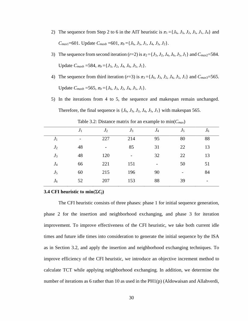
2) The sequence from Step 2 to 6 in the AIT heuristic is π1 ={J6, J3, J2, J5, J1, J4} and
Cmax1=601. Update Cmaxb =601, πb ={J6, J5, J1, J4, J3, J2}.
3) The sequence from second iteration (r=2) is π2 ={J3, J2, J4, J6, J5, J1} and Cmax2=584.
Update Cmaxb =584, πb ={J3, J2, J4, J6, J5, J1}.
4) The sequence from third iteration (r=3) is π3 ={J6, J3, J2, J4, J5, J1} and Cmax3=565.
Update Cmaxb =565, πb ={J6, J3, J2, J4, J5, J1}.
5) In the iterations from 4 to 5, the sequence and makespan remain unchanged.
Therefore, the final sequence is {J6, J3, J2, J4, J5, J1} with makespan 565.
Table 3.2: Distance matrix for an example to min(Cmax)
J1 J2 J3 J4 J5 J6
J1 - 227 214 95 80 88
J2 48 - 85 31 22 13
J3 48 120 - 32 22 13
J4 66 221 151 - 50 51
J5 60 215 196 90 - 84
J6 52 207 153 88 39 -
3.4 CFI heuristic to min(ƩCj)
The CFI heuristic consists of three phases: phase 1 for initial sequence generation,
phase 2 for the insertion and neighborhood exchanging, and phase 3 for iteration
improvement. To improve effectiveness of the CFI heuristic, we take both current idle
times and future idle times into consideration to generate the initial sequence by the ISA
as in Section 3.2, and apply the insertion and neighborhood exchanging techniques. To
improve efficiency of the CFI heuristic, we introduce an objective increment method to
calculate TCT while applying neighborhood exchanging. In addition, we determine the
number of iterations as 6 rather than 10 as used in the PH1(p) (Aldowaisan and Allahverdi,

31
2004) and LS (Laha and Sapkal, 2014) heuristics. Six iterations reduce the computation
time and maintain effectiveness of the CFI heuristic. The steps of the CFI heuristic are as
follows:
Step 1: Compute the distance matrix 𝐷𝐷𝑛𝑛×𝑛𝑛 and obtain the initial sequence π0 using
ISA. Let TCT0 be the total completion time of π0. Set the current best total
completion time TCTb=TCT0, the current best sequence πb=π0, and the
number of iterations r from 1 to 6 for Steps 2 to 6.
Step 2: Select first two jobs from πb, and choose the partial sequence with a smaller
TCT.
Step 3: First, apply the NEH insertion technique (Nawaz et al., 1983) to the obtained
partial sequences, select the best partial sequence with minimum TCT as
current sequence. Next, exchange the position of each job in the current
sequence with that of the rest jobs. Among sequences generated by
interchanging, the objective increment method is used to calculate ∆TCT. If
one sequence yields the smallest negative ∆TCT, set this sequence as the
current sequence, otherwise, keep the current one.
Step 4: Repeat Step 3 until all jobs are scheduled, and set the current sequence as πr
with TCTr.
Step 5: If TCTr< TCTb, set TCTb=TCTr and πb=πr.
Step 6: For j=1 to n–1, insert the jth job in πr into n–j possible positions in the forward
direction. If these sequences generate a lower TCT than TCTb, then update πb
and TCTb.

32
Step 7: Update r=r+1. If r≤6, return to Step 2; otherwise, go to Step 8. (Note: the
condition r≤6 is concluded from a case study.)
Step 8: Output the final πb and TCTb.
While using neighborhood exchanging technique in Step 3, an objective increment
method is introduced to calculate TCT. For example, there are five jobs scheduled and the
distance matrix D5×5 is computed. For the sequence π={J1, J2, J3, J4, J5},
TCTπ=5∑ 𝑝𝑝𝜋𝜋(1),𝑖𝑖𝑚𝑚𝑖𝑖=1 +∑ (𝑛𝑛 − 𝑗𝑗 + 1)𝐷𝐷𝜋𝜋(𝑗𝑗−1),𝜋𝜋(𝑗𝑗)
5𝑗𝑗=2 using Equation (3-7). Let J1 and J2 be
exchanged, and update the sequence as π’={J2, J1, J3, J4, J5}. The objective increment is
∆TCT = 5(∑ 𝑝𝑝2,𝑖𝑖𝑚𝑚𝑖𝑖=1 − ∑ 𝑝𝑝1,𝑖𝑖
𝑚𝑚𝑖𝑖=1 ) + 4(D2,1–D1,2) + 3(D1,3–D2,3). 𝑆𝑆𝐶𝐶𝑆𝑆𝜋𝜋′ = 𝑆𝑆𝐶𝐶𝑆𝑆𝜋𝜋 + ∆𝑆𝑆𝐶𝐶𝑆𝑆.
Therefore, using the objective increment method, the TCT can be calculated without
computing TCT for the whole sequence. The details of the objective increment method are
provided in section 3.5.
The main computational burden of the CFI heuristic is determined by the NEH
insertion and neighborhood exchanging techniques in Step 3. The computational
complexity for the NEH insertion is O(n3) including calculating TCT with O(n) when
selecting the best insertion position. The computational complexity for neighborhood
exchanging technique is also O(n3) including calculating TCT with O(1) when selecting
the best exchanged pair. Therefore, the overall computational complexity of the CFI
heuristic is O(n3), which is the same as that of the PH1(p) and LS heuristics, and less than
that of the FNM heuristic.
To illustrate the main steps of the CFI heuristic, we provide a 5-job 4-machine
instance as shown in Table 3.3, which is the same as in Bertolissi (2000).

33
• Initial sequence algorithm
Step 1: S=∅ and the U={J1, J2, J3, J4, J5}.
Step 2: Consider J1 in the 1st position of S, the processing times of J2, J3, J4, and J5 on
each machine are the average processing times. APTi = [18, 15.25, 13.75, 15.5].
Append this artificial job to J1, and we can obtain the current idle time of 48,
and future idle time of 13.25. The index function value for J1, namely f(1), is
205.25. We can consider J2 in the 1st position of S and obtain f(2)=211.
Similarly, we can obtain f(3)=199.25, f(4)=222.25, and f(5)=230.25. Hence, we
remove J3 that has the minimum f value from U and put it into the 1st position
of S.
Step 3: For the 2nd position in S, we can do the similar procedure as in Step 2, and
obtain the index function values f for each job in U, which are f = [155, 53.33,
153, 100.33]. Hence we remove J2 from U and put it into the 2nd position of S.
Similarly, we generate the initial sequence π0 as {J3, J2, J1, J5, J4}.
• CFI heuristic
The distance matrix 𝐷𝐷𝑛𝑛×𝑛𝑛 calculated by Equation (3-5) is shown in Table 3.4. From
the ISA, we obtain initial sequence π0 ={J3, J2, J1, J5, J4,} and TCT0=501. Set TCTb=501,
πb ={J3, J2, J1, J5, J4}, and r=1.
Table 3.3: Processing times of a 5-job 4-machine instance.
M1 M2 M3 M4
J1 12 24 12 13
J2 20 3 19 11
J3 19 20 3 15
J4 14 23 16 14
J5 19 15 17 22

34
We can select first two jobs, J3 and J2, from the initial sequence, and obtain a TCT
of 129 for a partial sequence {J3, J2}. Exchange the two jobs and obtain a TCT of 130 for
a partial sequence {J2, J3}. Hence, we fix the relative positions of two jobs as a partial
sequence of {J3, J2}.
Inserting J1 from the initial sequence to each possible position of the partial
sequence {J3, J2}, we can have the following partial sequences, {J1, J3, J2}, {J3, J1, J2} and
{J3, J2, J1} with partial TCTs of 228, 250, 229, respectively. Hence, we choose the partial
sequence of {J1, J3, J2} as the current sequence with the minimum partial TCT of 228. The
neighborhood exchanging method is applied, and the following partial sequences are
examined, {J3, J1, J2}, {J2, J3, J1} and {J1, J2, J3} with ∆𝑆𝑆𝐶𝐶𝑆𝑆𝑇𝑇 of 22, 10 and 13, respectively.
None of these values is lower than 0, therefore, the current sequence remains as {J1, J3, J2}.
Insert J5 from the initial sequence to each possible position of the current sequence,
and the following partial sequences are examined: {J5, J1, J3, J2}, {J1, J5, J3, J2}, {J1, J3, J5,
J2} and {J1, J3, J2, J5} with partial TCTs of 376, 376, 372, and 359, respectively. Hence,
we choose {J1, J3, J2, J5} as the current sequence with the minimum partial TCT of 359.
The neighborhood exchanging method is applied, and the following partial sequences are
examined: {J3, J1, J2, J5}, {J2, J3, J1, J5}, {J5, J3, J2, J1}, {J1, J2, J3, J5}, {J1, J5, J2, J3} and
Table 3.4: Distance matrix for an example to min(ƩCj)
J1 J2 J3 J4 J5
J1 - 17 15 28 29
J2 28 - 24 34 40
J3 31 15 - 35 36
J4 19 16 15 - 25
J5 13 11 15 14 -

35
{J1, J3, J5, J2} with ∆𝑆𝑆𝐶𝐶𝑆𝑆𝑇𝑇 of 36, 16, 36, 20, 18, and 13, respectively. None of these values
is lower than 0, therefore, the current sequence remains as {J1, J3, J2, J5}.
Insert J4 from the initial sequence to each possible position of the current sequence
and the following candidates are tried: {J4, J1, J3, J2, J5}, {J1, J4, J3, J2, J5}, {J1, J3, J4, J2,
J5}, {J1, J3, J2, J4, J5} and {J1, J3, J2, J5, J4} with TCTs of 526, 532, 542, 503 and 504.
Hence, we choose {J1, J3, J2, J4, J5} as the current sequence with minimum TCT of 503.
The neighborhood exchanging method is applied and the following partial sequences are
examined: {J3, J1, J2, J4, J5},{J2, J3, J1, J4, J5},{J4, J3, J2, J1, J5},{J5, J3, J2, J4, J1},{J1, J2,
J3, J4, J5},{J1, J4, J2, J3, J5},{J1, J5, J2, J4, J3},{J1, J3, J4, J2, J5},{J1, J3, J5, J4, J2},and {J1,
J3, J2, J5, J4} with ∆𝑆𝑆𝐶𝐶𝑆𝑆𝑇𝑇 of 50, 32, 22, 54, 37, 46, 34, 39, 14 and 1. None of these values
is lower than 0, therefore, the current sequence remains as {J1, J3, J2, J4, J5} with TCT 503.
After using insertion and neighborhood interchanging methods, we obtain π1={J1,
J3, J2, J4, J5} and TCT1=503. Since TCT1 is larger than TCTb, the πb remains unaltered with
TCTb 501. For j=1 to 4, insert jth job into each possible position of π1 in the forward
direction and get the following sequences: {J3, J1, J2, J4, J5}, {J3, J2, J1, J4, J5}, {J3, J2, J4,
J1, J5}, {J3, J2, J4, J5, J1}, {J1, J2, J3, J4, J5}, {J1, J2, J4, J3, J5}, {J1, J2, J4, J5, J3}, {J1, J3, J4,
J2, J5}, {J1, J3, J4, J5, J2} and {J1, J3, J2, J5, J4}.553, 510, 514, 510, 540, 541, 540, 542, 531,
and 504. None of these values is lower than TCTb, the πb remains unaltered with TCTb 501
and is used for further process till r=6 iterations are completed. Hence, the final sequence
is {J3, J2, J1, J5, J4} with TCT 501.
3.5 Objective increment method to calculate total completion time (TCT)
Assume there is a sequence π={J1, J2,…, Jj-1, Jj,…, Jn}, and the corresponding TCT
is TCTπ. When π(k) and π(j) (0<k<j≤n) in π are exchanged, the new sequence π’ is generated,

36
the difference of TCT between π’ and π, i.e., ∆𝑆𝑆𝐶𝐶𝑆𝑆(𝑘𝑘, 𝑗𝑗), can be calculated by one of the
following conditions:
Condition 1: k=1 and j=2
∆𝑆𝑆𝐶𝐶𝑆𝑆(𝑘𝑘, 𝑗𝑗) = 𝑛𝑛��𝑝𝑝𝜋𝜋′(𝑘𝑘),𝑖𝑖
𝑚𝑚
𝑖𝑖=1
−�𝑝𝑝𝜋𝜋(𝑘𝑘),𝑖𝑖
𝑚𝑚
𝑖𝑖=1
� + (𝑛𝑛 − 1)�𝐷𝐷𝜋𝜋′(𝑘𝑘),𝜋𝜋′(𝑗𝑗) − 𝐷𝐷𝜋𝜋(𝑘𝑘),𝜋𝜋(𝑗𝑗)�
+ (𝑛𝑛 − 2)�𝐷𝐷𝜋𝜋′(𝑗𝑗),𝜋𝜋′(𝑗𝑗+1) − 𝐷𝐷𝜋𝜋(𝑗𝑗),𝜋𝜋(𝑗𝑗+1)�
Condition 2: k=1 and j=3,…,n–1
∆𝑆𝑆𝐶𝐶𝑆𝑆(𝑘𝑘, 𝑗𝑗) = 𝑛𝑛��𝑝𝑝𝜋𝜋′(𝑘𝑘),𝑖𝑖
𝑚𝑚
𝑖𝑖=1
−�𝑝𝑝𝜋𝜋(𝑘𝑘),𝑖𝑖
𝑚𝑚
𝑖𝑖=1
�
+ (𝑛𝑛 − 1)�𝐷𝐷𝜋𝜋′(𝑘𝑘),𝜋𝜋′(𝑘𝑘+1) − 𝐷𝐷𝜋𝜋(𝑘𝑘),𝜋𝜋(𝑘𝑘+1)�
+ (𝑛𝑛 − 𝑗𝑗 + 1)� 𝐷𝐷𝜋𝜋′(𝑗𝑗−1),𝜋𝜋′(𝑗𝑗) − 𝐷𝐷𝜋𝜋(𝑗𝑗−1),𝜋𝜋(𝑗𝑗)� + (𝑛𝑛
− 𝑗𝑗)(𝐷𝐷𝜋𝜋′(𝑗𝑗)𝜋𝜋′(𝑗𝑗+1) − 𝐷𝐷𝜋𝜋(𝑗𝑗),𝜋𝜋(𝑗𝑗+1))
Condition 3: k=1 and j=n
∆𝑆𝑆𝐶𝐶𝑆𝑆(𝑘𝑘, 𝑗𝑗) = 𝑛𝑛��𝑝𝑝𝜋𝜋′(𝑘𝑘),𝑖𝑖
𝑚𝑚
𝑖𝑖=1
−�𝑝𝑝𝜋𝜋(𝑘𝑘),𝑖𝑖
𝑚𝑚
𝑖𝑖=1
�
+ (𝑛𝑛 − 1)�𝐷𝐷𝜋𝜋′(𝑘𝑘),𝜋𝜋′(𝑘𝑘+1) − 𝐷𝐷𝜋𝜋(𝑘𝑘),𝜋𝜋(𝑘𝑘+1)� + 𝐷𝐷𝜋𝜋′(𝑗𝑗−1),𝜋𝜋′(𝑗𝑗)
− 𝐷𝐷𝜋𝜋(𝑗𝑗−1),𝜋𝜋(𝑗𝑗)
Condition 4: k=2,3,…,n–2 and j=k+1
∆𝑆𝑆𝐶𝐶𝑆𝑆(𝑘𝑘, 𝑗𝑗) = (𝑛𝑛 − 𝑘𝑘 + 1)� 𝐷𝐷𝜋𝜋′(𝑘𝑘−1),𝜋𝜋′(𝑘𝑘) − 𝐷𝐷𝜋𝜋(𝑘𝑘−1),𝜋𝜋(𝑘𝑘)�
+ (𝑛𝑛 − 𝑘𝑘)� 𝐷𝐷𝜋𝜋′(𝑘𝑘),𝜋𝜋′(𝑗𝑗) − 𝐷𝐷𝜋𝜋(𝑘𝑘),𝜋𝜋(𝑗𝑗)�
+ (𝑛𝑛 − 𝑗𝑗)� 𝐷𝐷𝜋𝜋′(𝑗𝑗),𝜋𝜋′(𝑗𝑗+1) −𝐷𝐷𝜋𝜋(𝑗𝑗),𝜋𝜋(𝑗𝑗+1)�
Condition 5: k=2,3,…,n–3 and j=k+2,…,n–1

37
∆𝑆𝑆𝐶𝐶𝑆𝑆(𝑘𝑘, 𝑗𝑗) = (𝑛𝑛 − 𝑘𝑘 + 1)� 𝐷𝐷𝜋𝜋′(𝑘𝑘−1),𝜋𝜋′(𝑘𝑘) − 𝐷𝐷𝜋𝜋(𝑘𝑘−1),𝜋𝜋(𝑘𝑘)�
+ (𝑛𝑛 − 𝑘𝑘)� 𝐷𝐷𝜋𝜋′(𝑘𝑘),𝜋𝜋′(𝑘𝑘+1) −𝐷𝐷𝜋𝜋(𝑘𝑘),𝜋𝜋(𝑘𝑘+1)�
+ (𝑛𝑛 − 𝑗𝑗 + 1)� 𝐷𝐷𝜋𝜋′(𝑗𝑗−1),𝜋𝜋′(𝑗𝑗) − 𝐷𝐷𝜋𝜋(𝑗𝑗−1),𝜋𝜋(𝑗𝑗)�
+ (𝑛𝑛 − 𝑗𝑗)� 𝐷𝐷𝜋𝜋′(𝑗𝑗),𝜋𝜋′(𝑗𝑗+1) −𝐷𝐷𝜋𝜋(𝑗𝑗),𝜋𝜋(𝑗𝑗+1)�
Condition 6: k=2,3,…n–2 and j=n
∆𝑆𝑆𝐶𝐶𝑆𝑆(𝑘𝑘, 𝑗𝑗) = (𝑛𝑛 − 𝑘𝑘 + 1)� 𝐷𝐷𝜋𝜋′(𝑘𝑘−1),𝜋𝜋′(𝑘𝑘) − 𝐷𝐷𝜋𝜋(𝑘𝑘−1),𝜋𝜋(𝑘𝑘)�
+ (𝑛𝑛 − 𝑘𝑘)� 𝐷𝐷𝜋𝜋′(𝑘𝑘),𝜋𝜋′(𝑘𝑘+1) −𝐷𝐷𝜋𝜋(𝑘𝑘),𝜋𝜋(𝑘𝑘+1)� + 𝐷𝐷𝜋𝜋′(𝑗𝑗−1),𝜋𝜋′(𝑗𝑗)
− 𝐷𝐷𝜋𝜋(𝑗𝑗−1),𝜋𝜋(𝑗𝑗)
Condition 7: k=n–1 and j=n
∆𝑆𝑆𝐶𝐶𝑆𝑆(𝑘𝑘, 𝑗𝑗) = 2�𝐷𝐷𝜋𝜋′(𝑘𝑘−1),𝜋𝜋′(𝑘𝑘) − 𝐷𝐷𝜋𝜋(𝑘𝑘−1),𝜋𝜋(𝑘𝑘)� + 𝐷𝐷𝜋𝜋′(𝑘𝑘),𝜋𝜋′(𝑗𝑗) − 𝐷𝐷𝜋𝜋(𝑘𝑘),𝜋𝜋(𝑗𝑗)
Hence, the TCT of new sequence π’ can be calculated by the following equation:
𝑆𝑆𝐶𝐶𝑆𝑆𝜋𝜋′ = 𝑆𝑆𝐶𝐶𝑆𝑆𝜋𝜋 + ∆𝑆𝑆𝐶𝐶𝑆𝑆
Therefore, the calculation of TCT for the new sequence can be reduced from O(n)
to O(1).

38
Chapter 4 Case study
To test the performance of our proposed heuristics on Fm |nwt| Cmax and Fm |nwt|
ƩCj problems, we have done a series of case studies, and the results are presented in this
chapter. First, we provide the schemes to generate the data and evaluate the heuristic
performance. Second, for each single objective, the computational results of all compared
heuristics are given from the perspectives of effectiveness and efficiency. Third, we
introduce trade-off balancing function to evaluate of trade-off between min(Cmax) and
min(∑Cj) for each heuristic. Finally, statistical process control (SPC) is used to evaluate
the performance of the CFI heuristic along time horizon based on University of Kentucky
HealthCare historical data.
4.1 Schemes to carry out case studies
First, to evaluate the performance of the AIT heuristic on solving Fm |nwt| Cmax
problems, we compare the AIT heuristic with the LC (Laha and Chakraborty, 2009), ADT
(Ye et al., 2016) and CH (Li et al., 2008) heuristics. Second, to evaluate the performance
of the CFI heuristic on solving Fm |nwt| ∑Cj problems, we compare the CFI heuristic with
the PH1(p) (Aldowaisan and Allahverdi, 2004), the FNM (Framinan et al., 2010), and LS
(Laha and Sapkal, 2014) heuristics.
For effectiveness, we use the average relative percentage deviation (ARPD),
maximum percentage deviation (MPD), and percentage of the best solutions (PBS) to
evaluate each heuristic based on both small-scale and large-scale instances. Analysis of
variance (ANOVA) techniques and paired t-tests are used to statistically verify the
improvement on effectiveness based on large-scale instances. To evaluate efficiency, we

39
use the computation times based only on large-scale instances, as the computation times
for the small-scale instances are negligible.
For small-scale instances, the number of jobs is 5, 6, 7, or 8, and the number of
machines is 5, 10, 15, 20, or 25. Thus, there are 20 combinations. For each combination,
30 instances are generated randomly, and the processing times for each instance are
integers, following a uniform distribution in [1, 99]. In total, there are 600 instances in
small-scale.
For large-scale instances, Taillard’s benchmarks (Taillard, 1994) are classic and
commonly used to test the performance of heuristics for flow shop scheduling. Taillard’s
benchmarks consist of 120 instances in 12 combinations, with 10 instance for each
combination, where the number of jobs is 20, 50, 100, 200 or 500, and the number of
machines is 5, 10 or 20.
For Fm |nwt| Cmax problems, three criteria are used to evaluate the effectiveness of
each heuristic (Ye et al., 2016; Li et al., 2008):
(1) Average relative percent deviation (ARPD):
𝐴𝐴𝐴𝐴𝐴𝐴𝐷𝐷 =1𝑁𝑁�
𝑀𝑀𝑖𝑖(𝐻𝐻) − 𝐵𝐵𝐵𝐵𝑇𝑇𝐵𝐵𝑘𝑘𝑛𝑛𝑘𝑘𝑘𝑘𝑛𝑛𝑖𝑖𝐵𝐵𝐵𝐵𝑇𝑇𝐵𝐵𝑘𝑘𝑛𝑛𝑘𝑘𝑘𝑘𝑛𝑛𝑖𝑖
× 100𝑁𝑁
𝑖𝑖=1
(4-1)
(2) Maximum percent deviation (MPD):
𝑀𝑀𝐴𝐴𝐷𝐷 = max𝑖𝑖=1,…,𝑁𝑁
�𝑀𝑀𝑖𝑖(𝐻𝐻) − 𝐵𝐵𝐵𝐵𝑇𝑇𝐵𝐵𝑘𝑘𝑛𝑛𝑘𝑘𝑘𝑘𝑛𝑛𝑖𝑖
𝐵𝐵𝐵𝐵𝑇𝑇𝐵𝐵𝑘𝑘𝑛𝑛𝑘𝑘𝑘𝑘𝑛𝑛𝑖𝑖� × 100
(4-2)
where, 𝑀𝑀𝑖𝑖(𝐻𝐻) is the makespan obtained by heuristic H for an instance i in a
combination. N is the number of instances for each combination. N is 30 for small-
scale instances but is 10 for large-scale instances. 𝐵𝐵𝐵𝐵𝑇𝑇𝐵𝐵𝑘𝑘𝑛𝑛𝑘𝑘𝑘𝑘𝑛𝑛𝑖𝑖 is the optimal

40
solution for small-scale instances by using exhaustive enumeration. However, for
large-scale instances, 𝐵𝐵𝐵𝐵𝑇𝑇𝐵𝐵𝑘𝑘𝑛𝑛𝑘𝑘𝑘𝑘𝑛𝑛𝑖𝑖 is the best makespan among all four heuristics.
(3) Percentage of the best solutions (PBS)
PBS is the percentage of instances for which a heuristic achieves the best
performance among the four heuristics. The row total for PBS does not necessarily
sum to 100% since some heuristics may tie on the best performance for some
instances.
Similarly, for Fm |nwt| ∑Cj problems, three similar criteria are used to evaluate
effectiveness of each heuristic:
(1) Average relative percent deviation (ARPD):
𝐴𝐴𝐴𝐴𝐴𝐴𝐷𝐷 =1𝑁𝑁�
𝑆𝑆𝐶𝐶𝑆𝑆𝑖𝑖(𝐻𝐻)− 𝐵𝐵𝐵𝐵𝑇𝑇𝐵𝐵𝑘𝑘𝑛𝑛𝑘𝑘𝑘𝑘𝑛𝑛𝑖𝑖𝐵𝐵𝐵𝐵𝑇𝑇𝐵𝐵𝑘𝑘𝑛𝑛𝑘𝑘𝑘𝑘𝑛𝑛𝑖𝑖
× 100𝑁𝑁
𝑖𝑖=1
(4-3)
(2) Maximum percent deviation (MPD):
𝑀𝑀𝐴𝐴𝐷𝐷 = max𝑖𝑖=1,…,𝑁𝑁
�𝑆𝑆𝐶𝐶𝑆𝑆𝑖𝑖(𝐻𝐻) − 𝐵𝐵𝐵𝐵𝑇𝑇𝐵𝐵𝑘𝑘𝑛𝑛𝑘𝑘𝑘𝑘𝑛𝑛𝑖𝑖
𝐵𝐵𝐵𝐵𝑇𝑇𝐵𝐵𝑘𝑘𝑛𝑛𝑘𝑘𝑘𝑘𝑛𝑛𝑖𝑖� × 100 (4-4)
𝑆𝑆𝐶𝐶𝑆𝑆𝑖𝑖(𝐻𝐻) is the total completion time obtained by heuristic H for an instance i in a
combination. N is the number of instances for each combination. N is 30 for small-
scale instances but is 10 for large-scale instances. 𝐵𝐵𝐵𝐵𝑇𝑇𝐵𝐵𝑘𝑘𝑛𝑛𝑘𝑘𝑘𝑘𝑛𝑛𝑖𝑖 is the optimal
solution for small-scale instances by using the exhaustive enumeration method.
However, for large-scale instances, the best known solutions are from Qi et al.
(2016), who proposed the best known upper bounds for Fm |nwt| ∑Cj problems
based on Taillard’s benchmarks.
(3) Percentage of the best solutions (PBS)

41
PBS is the percentage of instances for which a heuristic achieves the best
performance among the four heuristics. The row total for PBS does not necessarily
sum to 100% since some heuristics may tie on the best performance for some
instances.
4.2 Results of case study on Fm |nwt| Cmax problems
4.2.1 Small-scale instances
For small-scale instances, the results are shown in Table 4.1. The AIT heuristic
achieves the best performance on ARPD of 0.23%, on MPD of 5.14%, and on PBS of
82.17%.
As shown in Table 4.1 for small-scale instances, with respect to ARPD, the CH
heuristic achieves an average of 0.30%, better than 1.28% of the LC heuristic and 0.62%
of the ADT heuristic. However, the AIT heuristic achieves the smallest average of 0.23%,
which has a 23.3% improvement over the CH heuristic. With regard to MPD, the CH
heuristic achieves 5.18%, smaller than 11.42% of the LC heuristic and 7.00% of the ADT
heuristic. The AIT heuristic also achieves the smallest MPD of 5.14%. With respect to
PBS, the CH heuristic achieves 76.50%, better than 63.33% and 48.5% of the ADT and
LC heuristics, respectively. However, the AIT heuristic achieves the best PBS of 82.17%.
Overall, the AIT heuristic achieves the best performances in ARPD, MPD and PBS in
small-scale instances, compared with the LC, ADT, and CH heuristics.

42
Table 4.1: Average Relative and Maximum percent deviations (ARPD & MPD) for
small-scale instances to min(Cmax) (%)
Size LC ADT CH AIT
n m ARPD MPD ARPD MPD ARPD MPD ARPD MPD
5 5 0.75 11.42 0.52 3.44 0.10 3.08 0.17 5.14
10 0.71 4.17 0.70 6.11 0.21 4.11 0.00 0.00
15 1.05 5.86 0.28 3.61 0.01 0.43 0.01 0.43
20 0.79 3.48 0.12 1.79 0.27 3.96 0.13 3.96
25 1.06 5.74 0.30 3.92 0.11 1.48 0.07 1.48
6 5 0.87 6.16 0.35 4.20 0.14 4.20 0.37 4.76
10 1.31 5.06 0.33 4.05 0.33 3.52 0.19 3.61
15 1.75 6.28 0.84 5.93 0.21 2.06 0.23 3.86
20 1.09 5.20 0.28 1.83 0.24 2.00 0.12 1.24
25 0.61 5.55 0.75 3.11 0.11 1.18 0.14 2.47
7 5 1.24 7.32 0.89 5.52 0.32 1.96 0.20 1.79
10 1.65 6.27 0.59 2.87 0.58 5.18 0.48 4.88
15 2.17 7.84 0.93 3.78 0.58 3.79 0.40 4.55
20 1.08 3.90 0.55 3.53 0.46 4.42 0.18 1.83
25 1.48 6.48 0.63 3.30 0.46 3.30 0.31 3.80
8 5 1.71 7.00 1.38 7.00 0.41 3.72 0.12 2.06
10 1.54 8.05 0.74 5.27 0.34 2.82 0.44 3.54
15 1.56 7.84 0.76 3.77 0.37 2.13 0.25 2.52
20 1.75 6.82 0.70 3.13 0.40 2.26 0.31 1.79
25 1.47 7.36 0.79 3.96 0.25 1.55 0.49 3.58
All instances 1.28 11.42 0.62 7.00 0.30 5.18 0.23 5.14
PBS 48.50 63.33 76.50 82.17

43
4.2.2 Large-scale instances
For large-scale instances, the results are shown in Table 4.2. The AIT heuristic
achieves the best performance on ARPD of 0.23% and on PBS of 65.83%, but not on MPD
of 2.95%.
Table 4.2: Average Relative and Maximum percent deviations (ARPD & MPD) for large-scale instances to min(Cmax) (%)
Size LC ADT CH AIT n m ARPD MPD ARPD MPD ARPD MPD ARPD MPD 20 5 2.20 3.89 2.21 5.38 0.97 2.28 0.24 0.99 10 3.09 6.14 2.26 4.45 0.58 2.22 0.80 2.95 20 2.09 6.46 0.92 3.07 1.04 2.32 0.61 1.91
50 5 3.24 4.72 3.68 4.97 0.78 2.14 0.07 0.68 10 2.40 4.11 2.24 3.90 0.66 1.69 0.06 0.49 20 2.69 6.27 1.33 2.12 0.36 1.46 0.26 1.26
100 5 2.85 4.24 4.29 5.20 0.47 1.12 0.20 1.47 10 2.91 4.20 2.00 2.77 0.50 1.06 0.05 0.50 20 2.38 3.77 1.32 1.91 0.26 1.21 0.25 0.94
200 10 2.57 3.26 2.04 3.05 0.50 1.61 0.13 0.47 20 2.51 3.22 1.48 2.10 0.46 0.92 0.06 0.41
500 20 2.67 3.39 1.89 2.53 1.10 1.71 0.00 0.00 All instances 2.63 6.46 2.14 5.38 0.64 2.32 0.23 2.95
PBS 0.83 5.83 29.17 65.83
As shown in Table 4.2, the LC heuristic achieves ARPD of 2.63%, MPD of 6.46%
and PBS of 0.83%. The ADT heuristic achieves ARPD of 2.14%, MPD of 5.38% and PBS
of 5.83%, better than the LC heuristic. The CH heuristic obtains ARPD of 0.64%, MPD of
2.32%, and PBS of 29.17%, and performs the best among the LC, ADT, and CH heuristics.
The AIT heuristic achieves the smallest ARPD of 0.23%, 64% improvement over the CH
heuristic. Besides, the AIT heuristic obtains the largest PBS of 65.83% among all four

44
heuristics, although the MPD of the AIT heuristic is 2.95%, close to 2.32% of the CH
heuristic, and smaller than those of the LC and ADT heuristics, which are 6.46% and 5.38%,
respectively.
ARPDs of heuristics for large-scale instances are used to plot the trend of deviations
as the number of jobs or machines increases, as shown in Figure 4.1.
(a) Deviation of Cmax by no. of jobs (%);
(b) Deviation of Cmax by no. of machines (%)
Figure 4.1: Deviations of Cmax as the number of jobs or machines increases

45
As the number of jobs increases from 20 to 500, Figure 4.1(a) shows that the
deviation of the AIT heuristic is smaller than those of other three heuristics. The trends of
the LC and ADT heuristics are relatively flat as the number of jobs increases. However, the
trend of the CH heuristic is going up when the number of jobs is larger than 100, whereas
the trend of the AIT heuristic is continuously going downwards as the number of jobs
increases.
Figure 4.1(b) plots the trend of ARPDs against the number of machines, ranging
from 5 to 20 machines. The trend obtained by the ADT heuristic continuously goes
downwards as the number of machines increases. However, the trends obtained by the LC,
CH and AIT heuristics are relatively flat, when the number of machines increases from 5
to 20. Among four heuristics, the deviation of the AIT heuristic is the smallest.
To verify the effectiveness of the AIT heuristic, two statistical analyses are
conducted based on ARPDs for large-scale instances. First, the analysis of variance
(ANOVA) is used to test the difference among the ARPDs of the LC, ADT, CH and AIT
heuristics. As shown in Table 4.3, the results show that the difference of ARPDs among
four heuristics is statistically significant at 95% confidence interval with p-value=0.000.
Second, paired t-tests on the ARPD are performed to validate whether there are
significant differences among the LC, ADT, CH and AIT heuristics. As shown in Table 4.4,
the estimates for mean differences between the AIT heuristic and other heuristics are all
Table 4.3: ANOVA results to min(Cmax) (95% Confidence Interval)
Source DF SS MS P
Heuristics 3 482.3 160.782 0.000
Error 476 437 0.918
Total 479 919.3

46
smaller than 0 with p-value=0.000, and the 95% confidence intervals for mean differences
fall into the negative interval, indicating that the ARPD of the AIT heuristic is significantly
smaller than those of other three heuristics at confidence level α=0.05.
We use the amount of CPU time to measure the efficiency of each heuristic. All
four heuristics are programmed in Matlab and run on a Dell Precision T1700 with Intel
Core i5-4590 CPUs of 3.3 GHz. For 500-job 20-machine instances, we have run one case
for 100 times and obtain the average CPU time, which is 38.31 seconds for the AIT
heuristic, and 21.97, 4.98, and 5.27 seconds for the CH, ADT, and LC heuristics,
respectively. The performance of the AIT heuristic on deviation justifies the additional
computation time, although the AIT heuristic uses the insertion and neighborhood
exchanging techniques and generates more sequences than the other three heuristics.
Overall, the AIT heuristic outperforms other heuristics on ARPD, MPD and PBS
criteria. Moreover, the deviation of makespan for the AIT heuristic has a decreasing trend
as the number of jobs or machines increases. Since all four heuristics have the same
computational complexity, the AIT heuristic statistically performs better than the other
three heuristics for no-wait flow shop production to min(Cmax).
4.3 Results of case study on Fm |nwt| ∑Cj problems
4.3.1 Small-scale instances
Table 4.4: Paired t-tests results to min(Cmax) (α=0.05)
AIT vs. LC ADT CH
p-value 0.000 0.000 0.000
Estimate for mean
difference –2.407 –1.911 –0.414
95% CI for mean difference (–2.618, –2.196) (–2.183, –1.639) (–0.574, –0.254)

47
For small-scale instances, the results are shown in Table 4.5. The CFI heuristic
achieves the best performance on ARPD of 0.06%, on MPD of 2.98%, and on PBS of 88%.
Table 4.5: Average relative and maximum percent deviation (ARPD & MPD) for
small-scale instances to min(∑Cj) (%)
Size PH1(p) FNM LS CFI
n m ARPD MPD ARPD MPD ARPD MPD ARPD MPD
5 5 0.41 5.94 0.18 2.08 0.18 2.09 0.05 1.36
10 0.13 1.36 0.09 1.93 0.06 1.36 0.06 0.79
15 0.27 2.77 0.28 3.38 0.07 0.77 0.01 0.30
20 0.07 0.43 0.03 0.43 0.01 0.24 0.01 0.24
25 0.06 1.31 0.01 0.41 0.04 1.31 0.04 1.02
6 5 0.46 3.93 0.24 3.93 0.06 0.75 0.01 0.37
10 0.38 5.61 0.38 5.61 0.20 2.43 0.01 0.32
15 0.28 4.11 0.20 2.33 0.26 4.11 0.12 2.33
20 0.40 3.09 0.16 0.98 0.25 3.09 0.02 0.29
25 0.16 1.69 0.05 0.93 0.03 0.64 0.00 0.00
7 5 0.51 5.99 0.30 1.95 0.23 1.95 0.03 0.54
10 0.50 2.60 0.22 1.20 0.31 2.00 0.06 1.82
15 0.46 4.65 0.14 0.92 0.34 3.71 0.12 1.28
20 0.49 3.76 0.34 2.54 0.25 2.52 0.08 1.11
25 0.16 0.98 0.09 0.87 0.21 1.97 0.05 0.85
8 5 0.53 3.07 0.39 3.21 0.35 1.98 0.25 2.98
10 0.40 3.86 0.34 3.64 0.42 3.64 0.11 1.01
15 0.61 3.47 0.44 3.47 0.31 2.19 0.13 1.19
20 0.50 2.77 0.41 1.81 0.32 1.81 0.08 0.69
25 0.57 2.80 0.28 2.80 0.23 2.32 0.07 0.72
All instances 0.37 5.99 0.23 5.61 0.21 4.11 0.06 2.98
PBS 65 73 75 88

48
As shown in Table 4.5 for small-scale instances, with respect to ARPD, the LS
heuristic achieves 0.21%, better than the PH1(p) heuristic of 0.37% and FNM heuristic of
0.23%. The CFI heuristic achieves the smallest ARPD of 0.06% from the optimal. With
regard to MPD, the LS heuristic achieves 4.11%, smaller than the PH1(p) of 5.99% and
FNM heuristic of 5.61%. The CFI heuristic also achieves the smallest MPD of 2.98%. With
respect to PBS, the LS and FNM heuristics are very close, 75% and 73%, respectively,
better than the PH1(p) heuristic of 65%. The CFI heuristic reaches 88% of the best solutions,
17% improvement over the LS heuristic.
4.3.2 Large-scale instances
For large-scale instances, the results are shown in Table 4.6. The CFI heuristic
achieves the best performance on ARPD of 2.08% and on PBS of 53%, but not on MPD of
7.05%.
As shown in Table 4.6, the PH1(p) heuristic achieves ARPD of 3.47%, MPD of
7.15% and PBS of 7%. The FNM heuristic achieves ARPD of 2.74%, MPD of 5.33% and
PBS of 12%, better than the PH1(p) heuristic. The LS heuristic obtains ARPD of 2.33%,
MPD of 4.91%, and PBS of 30%, better than the PH1(p) and FNM heuristics on
effectiveness. The CFI heuristic achieves the smallest ARPD of 2.08% and the largest PBS
of 53% among all four heuristics, although the MPD of the CFI heuristic is not as good as
the FNM and LS heuristics.

49
ARPDs of heuristics for large-scale instances are used to plot the trend of deviations
as the number of jobs or machines increases, as shown in Figure 4.2.
As the number of jobs increases from 20 to 500, Figure 4.2 (a) shows that the
deviations of all four heuristics are very close when the number of jobs is 20, and then
increase when the number of jobs changes from 20 to 100. In addition, as the number of
jobs increases from 100 to 500, the deviation of the CFI heuristic drops the fastest
compared with those of other three heuristics.
Figure 4.2 (b) plots the trend of ARPDs against the number of machines, ranging
from 5 to 20 machines. The trends obtained by the PH1(p) and LS heuristics go downwards
Table 4.6: Average relative and maximum percent deviation (ARPD & MPD) in
Taillard’s benchmark to min(∑Cj) (%)
Size PH1(p) FNM LS CFI
n m ARPD MPD ARPD MPD ARPD MPD ARPD MPD
20 5 1.60 5.21 1.27 2.55 1.38 3.26 0.87 3.03
10 1.36 3.25 1.61 3.89 1.06 2.92 1.34 3.52
20 1.50 4.43 1.13 2.87 0.85 2.30 0.74 1.47
50 5 4.02 6.84 3.31 5.33 2.38 4.91 2.19 4.12
10 3.03 5.51 3.03 4.76 2.02 3.82 2.14 3.69
20 2.69 4.35 2.79 4.88 1.97 4.19 1.35 1.91
100 5 5.94 7.15 3.44 4.55 3.75 4.72 3.35 5.35
10 4.58 5.43 3.41 4.63 2.87 4.73 3.07 7.05
20 3.89 5.18 3.19 3.97 2.61 3.37 2.53 4.89
200 10 4.98 6.04 3.84 4.16 3.61 4.44 3.49 4.30
20 4.47 5.12 3.67 4.60 2.96 4.01 2.88 4.38
500 20 3.62 4.86 2.21 2.41 2.50 3.11 0.98 1.78
All instances 3.47 7.15 2.74 5.33 2.33 4.91 2.08 7.05
PBS 7 12 30 53

50
as the number of machines increases from 5 to 15, whereas the deviations of both the FNM
and CFI heuristics go up. However, when the number of machines increases from 10 to 20,
the deviation of the CFI heuristic drops faster than those of other heuristics and reaches to
the lowest point of deviations.
(a) Deviation of TCT by no. of jobs (%);
(b) Deviation of TCT by no. of machines (%)
Figure 4.2: Deviations of TCT as the number of jobs or machines increases

51
To verify effectiveness of the CFI heuristic, two statistical analyses are conducted
based on the large-scale instances. Firstly, the analysis of variance (ANOVA) is used to
test whether the ARPDs of the PH1(p), FNM, LS and CFI heuristics are the same or
whether some ARPDs are different. The ANOVA results from Table 4.7 show that the
difference among heuristics is statistically significant with p-value=0.000.
Secondly, paired t-tests on the ARPD are performed to validate whether or not there
are significant differences among the PH1(p), FNM, LS and CFI heuristics. Table 4.8
shows the summarized results of the paired t-test for confidence level α=0.05. As Table 4.8
indicates, the CFI heuristic significantly outperforms the other three heuristics.
Computation times are used to evaluate efficiency of each heuristic. All four
heuristics are programmed in Matlab and run on a Dell Precision T1700 with Intel Core i5-
4590 CPUs of 3.3 GHz.
Table 4.7: ANOVA results to min(∑Cj) (95% Confidence Interval)
Source DF SS MS P
Heuristics 3 134.27 44.76 0.000
Error 476 890.40 1.87
Total 479 1024.68
Table 4.8: Paired t-test results to min(∑Cj) (α=0.05)
CFI vs. PH1(p) FNM LS
p-value 0.000 0.000 0.012
Estimate for mean
difference –1.397 –0.664 –0.2517
95% CI for mean difference (–1.659,–1.135) (–0.886,–0.442) (–0.4461,–0.0573)

52
Figure 4.3: The deviation from upper bound with the value of r
In order to improve efficiency of the CFI heuristic, we determine the number of
iterations r by changing r from 1 to 16 based on large-scale instances. We calculate the
deviations from upper bound for each value of r. Figure 4.3 indicates that when the value
of r is larger than or equal to 6, the deviation asymptotically reaches to the same level of
2.08%, which means our CFI heuristic generates all possible sequences in 6 iterations.
Therefore, we set the number of iterations r as 6.
The average computation time (in seconds) required for large-scale instances by
each heuristic is given in Table 4.9. On average, the CFI heuristic uses less CPU time than
the LS heuristic, but more CPU time than the PH1(p) and FNM heuristics. Although the
computational complexity of the FNM heuristic is O(n4), higher than that of the LS and
CFI heuristics, respectively, the FNM heuristic takes less computation time, because there
are 10 iterations in the LS heuristic and 6 in our CFI heuristic. Overall, the CFI heuristic
achieves the best effectiveness in less computation time among three popular heuristics.

53
(Unit: seconds)
4.4 Trade-off balancing
For bi-objective optimization of Cmax and ∑Cj, we introduce the trade-off balancing
function to evaluate the performance of each heuristic. The trade-off balancing function is
shown in Equation (4-5) as follows:
𝑆𝑆𝑇𝑇𝐵𝐵(𝛼𝛼) = 𝛼𝛼𝐶𝐶𝑚𝑚𝑚𝑚𝑚𝑚𝑁𝑁 + (1 − 𝛼𝛼)𝑆𝑆𝐶𝐶𝑆𝑆𝑁𝑁 (4-5)
Where the 𝛼𝛼 is the preference or weight for the objective of Cmax, 𝐶𝐶𝑚𝑚𝑚𝑚𝑚𝑚𝑁𝑁 is the
normalized value of Cmax and 𝑆𝑆𝐶𝐶𝑆𝑆𝑁𝑁 is the normalized value of TCT. We compare our AIT
heuristic and CFI heuristic with LS and CH heuristics based on large-scale instances. We
have chosen 𝛼𝛼 to be 0, 0.25, 0.5, 0.75, and 1. If 𝛼𝛼 is less than 0.5, we give more preference
to TCT and give more preference to Cmax when 𝛼𝛼 is greater than 0.5. The following Figure
4.4 shows how the performances of each heuristic behave given different value of 𝛼𝛼.
Table 4.9: CPU times of four heuristics for large-scale instances to min(∑Cj)
n m PH1(p) FNM LS CFI
20 5 0.00 0.02 0.10 0.06
10 0.00 0.01 0.10 0.05
20 0.00 0.01 0.09 0.06
50 5 0.02 0.10 0.71 0.44
10 0.02 0.10 0.72 0.44
20 0.02 0.10 0.72 0.46
100 5 0.09 0.80 4.10 2.66
10 0.10 0.83 4.23 2.78
20 0.12 0.86 4.17 2.81
200 10 0.69 9.24 28.78 19.26
20 0.77 9.38 28.65 19.51
500 20 10.64 283.49 467.04 319.58
All instances 1.04 25.41 44.95 30.68

54
(a) The trade-off balancing when 𝛼𝛼 = 0
(b) The trade-off balancing when 𝛼𝛼 = 0.25
0
0.2
0.4
0.6
0.8
1
1.2
20 50 100 200 500
TOB
No. of Job
α=0
LS
CH
AIT
CFI
0
0.1
0.2
0.3
0.4
0.5
0.6
0.7
0.8
0.9
20 50 100 200 500
TOB
No. of Job
α=0.25
LS
CH
AIT
CFI

55
(c) The trade-off balancing when 𝛼𝛼 = 0.5
(d) The trade-off balancing when 𝛼𝛼 = 0.75
0
0.1
0.2
0.3
0.4
0.5
0.6
0.7
0.8
20 50 100 200 500
TOB
No. of Job
α=0.5
LS
CH
AIT
CFI
0
0.1
0.2
0.3
0.4
0.5
0.6
0.7
0.8
0.9
20 50 100 200 500
TOB
No. of Job
α=0.75
LS
CH
AIT
CFI

56
(e) The trade-off balancing when 𝛼𝛼 = 1
Figure 4.4: The performances of each heuristic given different values of 𝛼𝛼
From Figure 4.4, given different values of 𝛼𝛼, we can see that both AIT and CFI
heuristics obtain the best performance. When the preference is given more to Cmax, the AIT
heuristic performs the best. When the preference is given more to the TCT, the CFI heuristic
performs the best. Besides, the trends obtained by the AIT and CFI heuristics go
downwards as the number of jobs increases from 20 to 500, whereas the trends of both the
LS and CH heuristics go up. In addition, when the number of job is 500, the performances
of AIT and CFI heuristic almost converge together, which indicates that the initial sequence
algorithm (ISA) plays an important role to generate the final solutions, since both heuristics
use the same ISA to generate initial sequence. Overall, our proposed heuristics have better
performances to minimize the trade-off than the other two heuristics.
4.5 Case study on UKHC historical data
To validate our CFI heuristic for operating room (OR) scheduling across the periop
process in a healthcare system, we carry out a case study based on historical OR data from
0
0.2
0.4
0.6
0.8
1
1.2
20 50 100 200 500
TOB
No. of Job
α=1
LS
CH
AIT
CFI

57
University of Kentucky HealthCare (UKHC), in which the first come first serve (FCFS)
rule is used for OR scheduling, especially for emergencies.
The historical data set obtained from UKHC consists of almost 30,000 cases in 365
consecutive days from 2013 to 2014. UKHC schedules operating rooms on weekdays, and
opens emergency rooms on weekends and holidays, thus the number of cases on weekends
and holidays is much less than that on weekdays. Therefore, removing data on weekends
and holidays, we have more than 27,000 cases in 50 weeks with 5 days a week, i.e., in 250
days. First, we compare the sequences of the PH1(p), FNM, LS, and CFI heuristics with
the UKHC ones based on average patient flow time (APFT), which equals to the total
completion time divided by the number of patients served in a day. Second, we use
statistical process control (SPC) techniques to compare the process capability based on
APFTs generated by our CFI heuristic and the actual UKHC data.
Table 4.10 shows the APFTs and standard deviations for four heuristics and the
actual UKHC data. As shown in Table 4.10, our CFI heuristic can achieve the smallest
APFT with the smallest standard deviation.
Table 4.10: APFT (minutes) and standard deviation for four heuristics and UKHC
PH1(p) FNM LS CFI UKHC
APFT 545.19 544.83 544.91 544.74 613.09
Standard deviation 40.91 40.85 40.88 40.82 56.20
Using SPC techniques, we generate process capabilities for both CFI and the
UKHC data as shown in Figure 4.5. The user-defined lower specification limit (LSL) and
upper specification limit (USL) are set as 400 and 700 minutes, respectively, according to
the historical data from UKHC. The process capabilities cp and cpk are defined as 𝑐𝑐𝑝𝑝 =
𝑈𝑈𝑈𝑈𝑈𝑈−𝑈𝑈𝑈𝑈𝑈𝑈6𝜎𝜎
and 𝑐𝑐𝑝𝑝𝑘𝑘 = min(𝑈𝑈𝑈𝑈𝑈𝑈−𝜇𝜇3𝜎𝜎
, 𝜇𝜇−𝑈𝑈𝑈𝑈𝑈𝑈3𝜎𝜎
), where µ is the average patient flow time and σ is

58
the standard deviation for the process performance (Montgomery, 2007). Process
capability cp indicates if the outcomes of a process are within the control limits. With the
fixed range of specification limits, which is USL − LSL, the larger the cp, the less the
variation in process, which is 6σ. Process capability index cpk indicates if the outcomes are
centered around the average performance. The larger the cpk, the less likely that the
outcomes will fall outside the limits, LSL or USL. As shown in Figure 4.5, the cp is 1.21
for our CFI heuristic and 0.90 for the UKHC data, and the cpk is 1.17 for our CFI heuristic
and 0.52 for the UKHC data. Obviously, the APFTs generated by our CFI heuristic are
more centered within the specification limits and with less variation, compared to those
from historical UKHC data.

59
(a) Process Capability of CFI
(b) Process Capability of UKHC
Figure 4.5: Capability analysis of average patient flow times in 250 days
Moreover, we generate the Xbar-R charts based on APFTs in 250 days as shown in
Figure 4.6. The APFT is 544.7 minutes for our CFI heuristic, and 613.1 minutes for the
data from UKHC. The improvement in average patient flow times can be calculated by
(613.1 − 544.7)/613.1=11.2%. The range of variation on our CFI heuristic is 205.5 minutes,
less than that of 275.4 minutes for the UKHC data.

60
(a) By CFI
(b) By UKHC
Figure 4.6: X-bar&R charts of average patient flow times
These results from X-bar&R charts support those of cp and cpk, and the 11.2%
improvement in average patient flow time indicates that potentially 3,000 additional
patients could be served in a year if our CFI heuristic was applied for sequencing. However,
in practice, OR scheduling and control is affected by many other factors in addition to

61
sequencing, such as emergencies, the availability of patients in the waiting list, surgical
staff, and equipment, etc. These realities are reflected in the UKHC data.
Based on the above case studies, we have test the effectiveness, efficiency and
robustness of our AIT and CFI heuristics. Compared with the best known heuristics for Fm
|nwt| Cmax and Fm |nwt| ƩCj problems, such as LC, ADT and CH heuristics for Cmax and
PH1(p), FNM and LS heuristics for ƩCj, our heuristics outperform them significantly. In
addition, for bi-objective optimization, our heuristics perform better than others based on
the trade-off balancing function. Last, compared with actual performance at UKHC, our
CFI heuristic can potentially serve 3,000 additional patients.
62
Chapter 5 Conclusion and future work
5.1 Concluding remarks
ORs are the largest cost center and the greatest revenue source simultaneously for
hospitals (Ghazalbash et al, 2012). To achieve high utilization of OR units and reduce
average waiting times are two main objectives in the 3-stage periop process. In the 3-stage
periop process, the performance of one stage affects the performances of adjacent stages,
which is also characteristic of a three-stage no-wait flow shop. The upstream stages affect
downstream stages to influence the utilization and patient flow, and downstream stages can
affect upstream stages as well, such as blocking and PACU boarding. Therefore, the 3-
stage no-wait flow shop is suitable to model the periop process, in which no waiting time
between stages is allowed.
No-wait flow shop production is common in industry, where no waiting time is
allowed between intermediate operations. Minimization of makespan (Cmax), which relates
to utilizations, for no-wait flow shop production has been proven to be NP-hard and
minimization of total completion time (∑Cj), which relates to average waiting time, has
been proven to be NP-complete. It is extremely time consuming to find optimal solutions
using exact methods for such problems. Therefore, heuristics are widely used to find near
optimal solutions for production scheduling in manufacturing. To min(Cmax), the LC, ADT,
and CH heuristics are three typical ones developed recently (Laha and Chakraborty, 2009,
Ye et al., 2016; Li et al., 2008), and to min(∑Cj), the PH1(p), FNM, and LS heuristics are
three typical ones in the literature (Aldowaisan and Allahverdi, 2004; Framinan et al., 2010;
Laha et al., 2014). These heuristics can obtain good solutions in a reasonable time, even
for large-scale instances. However, there are some shortcomings of their heuristics, such

63
as high computational complexity in the FNM heuristic, lack of large-scale computational
experiment in the LS heuristic.
To enhance effectiveness and efficiency beyond these heuristics, we propose the
AIT heuristic to min(Cmax) and the CFI heuristic to min(∑Cj) for no-wait flow shop
production. To improve effectiveness, we first take the current idle times and future idle
times into consideration, proposing an initial sequence algorithm, and then use the insertion
and neighborhood exchanging methods to further improve the solutions.
To increase efficiency, we first introduce an objective increment method to reduce
the computational complexity from O(n) to O(1) in calculating total completion time, and
then set the number of iterations in our AIT and CFI heuristic to further reduce the
computation times.
Compared with the LC, ADT and CH heuristics for the Fm |nwt| Cmax problems,
based on 600 small-scale instances, our AIT heuristic achieves the best performance on
average relative percentage deviation (ARPD) of 0.23%, maximum percentage deviation
(MPD) of 5.14%, and the percentage of the best solutions (PBS) of 82.17%. Based on
large-scale instances in Taillard’s benchmarks, our AIT heuristic achieves the best
performance on ARPD of 0.23% and PBS of 65.83%, although not on the MPD of 2.95%.
Compared with the PH1(p), FNM and LS heuristics for the Fm |nwt| ∑Cj problems,
based on 600 small-scale instances, our CFI heuristic achieves the best performance on
ARPD of 0.06%, MPD of 2.98%, and PBS of 88%. Based on large-scale instances in
Taillard’s benchmarks, our CFI heuristic achieves the best performance on ARPD of 2.08%
and PBS of 53%, although not on the MPD of 7.05%. In addition, on average, the CPU

64
time of our CFI heuristic is 30.68 seconds, based on Taillard’s benchmarks, less than the
44.95 seconds of the LS heuristic.
In the trade-off balancing, our AIT and CFI heuristics outperform the LS and CH
heuristics. When the preference is given more to Cmax, the AIT heuristic performs the best.
When the preference is given more to the ∑Cj, the CFI heuristic performs the best. Besides,
the trends obtained by the AIT and CFI heuristics go downwards as the number of jobs
increases from 20 to 500, whereas the trends of both the LS and CH heuristics go up.
In a case study using historical data from UKHC, we found our CFI heuristic can
achieve 11.2% improvement in average patient flow times over UKHC’s performance, and
the average patient flow times generated by our CFI heuristic are under better process
control with less variation. This means additional patients can potentially be served and
there is a greater control of OR management across the peri-operative process.
Overall, our AIT and CFI heuristics can achieve good effectiveness and efficiency
for no-wait flow shop scheduling and operating room scheduling.
5.2 Future work
Variation in processing times is a common disturbance to flow shop production in
manufacturing or healthcare systems, which consequently generates an uneven workflow
on the production lines. Cao, Patterson, and Bai (2005) have concluded that the main source
of variations in processing time is the variation in actual processing times from their
expected values. The difficulty to handle the variation in processing time is that we do not
exactly know how the current variations and performance will impact on the future overall
performance. One topic of our future work is adaptive production control by resequencing

65
jobs for this type of disturbances that the overall system performance can be under control
in an acceptable range.
Besides variations in processing time, there are trade-offs between different
objectives. Li et al. (2014) proved that the objectives of min(Cmax) and min(∑Cj) are not
consistent in traditional permutation flow shop scheduling problems. The limitation of
current work focuses on the evaluation scheme of trade-off for each single-objective
heuristic, not addressing the root causes of trade-offs in no-wait flow shop production
scheduling. The root cause of trade-off in flow shop scheduling is unbalanced cycle time
at different stages in production lines. Therefore, another topic of our future work is to
establish effective and efficient heuristics for multi-objective optimization in no-wait flow
shop based on balancing cycle times at each stage.
The third topic of our future work is to apply these heuristics to the hybrid no-wait
flow shop, in which there exist parallel machines at each stage. Based on the second future
work, we want to extend 3-machine flow shop to hybrid no-wait flow shop, which relates
to the resource allocation at each stage. On the one hand, from the second topic of future
work, we can find how sequencing changes the cycle time in no-wait flow shop scheduling.
On the other hand, different schemes of resource allocation affect the cycle time of each
machine at each stage as well. Therefore, it is important and meaningful to study the
following three questions: (1) given the fixed resources, how sequencing affects cycle time?
(2) Given the fixed sequencing method, how can we obtain better performances by
adjusting the resource allocation scheme? (3) How do the resource allocation scheme and
sequencing interact with each other to affect the performance of the systems?

66
Overall, the future work will focus on achieving adaptive scheduling in operating
rooms scheduling when (1) disturbances occur in systems; (2) optimizing different
inconsistent objectives, and (3) resource allocation and sequencing interact with each other.

67
References:
Allahverdi, A., and Aldowaisan, T. (2002). No-wait flowshops with bicriteria of makespan
and total completion time. Journal of the Operational Research Society, 53(9), 1004-
1015.
Aldowaisan, T., and Allahverdi, A. (2004). New heuristics for m-machine no-wait
flowshop to minimize total completion time. Omega, 32(5), 345-352.
Allahverdi, A., and Aldowaisan, T. (2004). No-wait flowshops with bicriteria of makespan
and maximum lateness. European Journal of Operational Research, 152(1), 132-147.
Augusto, V., Xie, X., and Perdomo, V. (2010). Operating theatre scheduling with patient
recovery in both operating rooms and recovery beds. Computers & Industrial
Engineering, 58(2), 231-238.
Banditori, C., Cappanera, P., and Visintin, F. (2013). A combined optimization–simulation
approach to the master surgical scheduling problem. IMA Journal of Management
Mathematics, 24(2), 155-187.
Beck, R., Pahlke, I., and Seebach, C. (2014). Knowledge exchange and symbolic action in
social media-enabled electronic networks of practice: A multilevel perspective on
knowledge seekers and contributors. MIS quarterly, 38(4), 1245-1270.
Benneyan, J. C., Lloyd, R. C., and Plsek, P. E. (2003). Statistical process control as a tool
for research and healthcare improvement. Quality and Safety in Health Care, 12(6),
458-464.
Bertolissi, E. (2000). Heuristic algorithm for scheduling in the no-wait flow-shop. Journal
of Materials Processing Technology, 107(1), 459-465.

68
Bonney, M. C., and Gundry, S. W. (1976). Solutions to the constrained flowshop
sequencing problem. Journal of the Operational Research Society, 27(4), 869-883.
Bosse, G., Mtatifikolo, F., Abels, W., Strosing, C., Breuer, J. P., and Spies, C. (2013).
Immediate outcome indicators in perioperative care: a controlled intervention study
on quality improvement in hospitals in Tanzania. PloS one, 8(6), e65428.
Cao, Q., Patterson, J. W., and Bai, X. (2005). Reexamination of processing time uncertainty.
European journal of operational research, 164(1), 185-194.
Cardoen, B., Demeulemeester, E., and Beliën, J. (2010). Operating room planning and
scheduling: A literature review. European journal of operational research, 201(3),
921-932.
Chen, C. L., Neppalli, R. V., and Aljaber, N. (1996). Genetic algorithms applied to the
continuous flow shop problem. Computers & Industrial Engineering, 30(4), 919-929.
Dannenbring, D. G. (1977). An evaluation of flow shop sequencing heuristics.
Management science, 23(11), 1174-1182.
Davis, K., Mazzuchi, T., and Sarkani, S. (2013). Architecting technology transitions: A
sustainability‐oriented sociotechnical approach. Systems Engineering, 16(2), 193-
212.
Deming, W. E. (2000). Out of the Crisis. MIT press.
Denton, B., Viapiano, J., and Vogl, A. (2007). Optimization of surgery sequencing and
scheduling decisions under uncertainty. Health care management science, 10(1), 13-
24.

69
Ding, J., Song, S., Zhang, R., and Wu, C. (2014, July). Minimizing makespan for a no-wait
flowshop using tabu mechanism improved iterated greedy algorithm. In Evolutionary
Computation (CEC), 2014 IEEE Congress on (pp. 1906-1911). IEEE.
Etzioni, D. A., Liu, J. H., Maggard, M. A., and Ko, C. Y. (2003). The aging population and
its impact on the surgery workforce. Annals of surgery, 238(2), 170-177.
Fink, A., and Voß, S. (2003). Solving the continuous flow-shop scheduling problem by
metaheuristics. European Journal of Operational Research, 151(2), 400-414.
Framinan, J. M., and Nagano, M. S. (2008). Evaluating the performance for makespan
minimisation in no-wait flowshop sequencing. Journal of materials processing
technology, 197(1), 1-9
Framinan, J. M., Nagano, M. S., and Moccellin, J. V. (2010). An efficient heuristic for total
flowtime minimisation in no-wait flowshops. The International Journal of Advanced
Manufacturing Technology, 46(9-12), 1049-1057.
Gao, K. Z., Pan, Q. K., and Li, J. Q. (2011). Discrete harmony search algorithm for the no-
wait flow shop scheduling problem with total flow time criterion. The International
Journal of Advanced Manufacturing Technology, 56(5-8), 683-692.
Gao, K., Pan, Q., Suganthan, P. N., and Li, J. (2013). Effective heuristics for the no-wait
flow shop scheduling problem with total flow time minimization. The International
Journal of Advanced Manufacturing Technology, 66(9-12), 1563-1572.
Gangadharan, R., and Rajendran, C. (1993). Heuristic algorithms for scheduling in the no-
wait flowshop. International Journal of Production Economics, 32(3), 285-290.
Garey, M. R., and Johnson, D. S. (2002). Computers and intractability: a guide to the theory
of NP-completeness. New York: freeman.

70
Ghazalbash, S., Sepehri, M. M., Shadpour, P., and Atighehchian, A. (2012). Operating
room scheduling in teaching hospitals. Advances in Operations Research, 2012, 16
pages.
Glouberman, S., and Mintzberg, H. (2001). Managing the care of health and the cure of
disease—Part I: Differentiation. Health care management review, 26(1), 56-69.
Graham, R. L., Lawler, E. L., Lenstra, J. K., and Kan, A. R. (1979). Optimization and
approximation in deterministic sequencing and scheduling: a survey. Annals of
discrete mathematics, 5, 287-326.
Gupta, D. (2007). Surgical suites' operations management. Production and Operations
Management, 16(6), 689-700.
Gupta, D., and Denton, B. (2008). Appointment scheduling in health care: Challenges and
opportunities. IIE transactions, 40(9), 800-819.
Hall, M. J., and Owings, M. (2014). Rural and urban hospitals’ role in providing inpatient
care, 2010. Population, 17, 12.
Ishibuchi, H., and Murata, T. (1998). A multi-objective genetic local search algorithm and
its application to flowshop scheduling. IEEE Transactions on Systems, Man, and
Cybernetics, Part C (Applications and Reviews), 28(3), 392-403.
Ishibuchi, H., Yoshida, T., and Murata, T. (2003). Balance between genetic search and
local search in memetic algorithms for multiobjective permutation flowshop
scheduling. IEEE transactions on evolutionary computation, 7(2), 204-223.
Javadi, B., Saidi-Mehrabad, M., Haji, A., Mahdavi, I., Jolai, F., and Mahdavi-Amiri, N.
(2008). No-wait flow shop scheduling using fuzzy multi-objective linear
programming. Journal of the Franklin Institute, 345(5), 452-467.

71
Johnson, S. M. (1954). Optimal two-and three-stage production schedules with setup times
included. Naval Research Logistics (NRL), 1(1), 61-68.
Kalczynski, P. J., and Kamburowski, J. (2007). On the NEH heuristic for minimizing the
makespan in permutation flow shops. Omega, 35(1), 53-60.
King, J. R., and Spachis, A. S. (1980). Heuristics for flow-shop scheduling. International
Journal of Production Research, 18(3), 345-357.
Laha, D., and Chakraborty, U. K. (2009). A constructive heuristic for minimizing
makespan in no-wait flow shop scheduling. The International Journal of Advanced
Manufacturing Technology, 41(1-2), 97-109.
Laha, D., Gupta, J. N., and Sapkal, S. U. (2014). A penalty-shift-insertion-based algorithm
to minimize total flow time in no-wait flow shops. Journal of the Operational
Research Society, 65(10), 1611-1624.
Laha, D., and Sapkal, S. U. (2014). An improved heuristic to minimize total flow time for
scheduling in the m-machine no-wait flow shop. Computers & Industrial Engineering,
67, 36-43.
Li, X., Wang, Q., and Wu, C. (2008). Heuristic for no-wait flow shops with makespan
minimization. International Journal of Production Research, 46(9), 2519-2530.
Li, W., and Freiheit, T. I. (2016). An effective heuristic for adaptive control of job
sequences subject to variation in processing times. International Journal of
Production Research, 54(12), 3491-3507.
Li, W., Nault, B. R., Xue, D., and Tu, Y. (2011). An efficient heuristic for adaptive
production scheduling and control in one-of-a-kind production. Computers &
Operations Research, 38(1), 267-276.

72
Li, W., Mitchell, V. L., and Nault, B. R. (2014, January). Inconsistent Objectives in
Operating Room Scheduling. In IIE Annual Conference. Proceedings (p. 727).
Institute of Industrial Engineers-Publisher.
Liao, X. P., Deng, J., and Li, X. P. (2008, July). An evolutionary algorithm for constraint
flow shops with multi-criteria optimization. In Machine Learning and Cybernetics,
2008 International Conference on (Vol. 2, pp. 904-908). IEEE.
Liu, Y. G., Zhu, X., and Li, X. P. (2008, July). A new hybrid genetic algorithm for the bi-
criteria no-wait flowshop scheduling problem with makespan and total flow time
minimization. In Machine Learning and Cybernetics, 2008 International Conference
on (Vol. 2, pp. 883-888). IEEE.
Liu, Jiyin, and Colin R. Reeves. "Constructive and composite heuristic solutions to the P//
∑ Ci scheduling problem." European Journal of Operational Research 132.2 (2001):
439-452.
Little, J. D. (1961). A proof for the queuing formula: L= λ W. Operations research, 9(3),
383-387.
Magerlein, J. M., and Martin, J. B. (1978). Surgical demand scheduling: a review. Health
services research, 13(4), 418.
Marcon, E., and Dexter, F. (2006). Impact of surgical sequencing on post anesthesia care
unit staffing. Health Care Management Science, 9(1), 87-98.
Meskens, N., Duvivier, D., and Hanset, A. (2013). Multi-objective operating room
scheduling considering desiderata of the surgical team. Decision Support Systems,
55(2), 650-659.

73
Moccellin, J. V. (1995). A new heuristic method for the permutation flow shop scheduling
problem. Journal of the Operational research Society, 46(7), 883-886.
Montgomery, D. C. (2007). Introduction to statistical quality control. John Wiley & Sons.
Moore, B., Levit, K., and Elixhauser, A. (2014). Costs for Hospital Stays in the United
States, 2012. HCUP Statistical Brief, 181.
Murata, T., Ishibuchi, H., and Tanaka, H. (1996). Genetic algorithms for flowshop
scheduling problems. Computers & Industrial Engineering, 30(4), 1061-1071.
Nawaz, M., Enscore, E. E., and Ham, I. (1983). A heuristic algorithm for the m-machine,
n-job flow-shop sequencing problem. Omega, 11(1), 91-95.
Ogbu, F. A., and Smith, D. K. (1990). The application of the simulated annealing algorithm
to the solution of the n/m/Cmax flowshop problem. Computers & Operations
Research, 17(3), 243-253.
Pan, Q. K., Wang, L., and Qian, B. (2008). A novel multi-objective particle swarm
optimization algorithm for no-wait flow shop scheduling problems. Proceedings of
the Institution of Mechanical Engineers, Part B: Journal of Engineering Manufacture,
222(4), 519-539.
Pan, Q. K., Wang, L., and Qian, B. (2009). A novel differential evolution algorithm for bi-
criteria no-wait flow shop scheduling problems. Computers & Operations Research,
36(8), 2498-2511.
Pellegrino, G. (2015). Obsolescence, presentification, revolution: Sociotechnical discourse
as site for in fieri futures. Current Sociology, 63(2), 216-227.
Pinedo, M.L. (2014). Scheduling: theory, algorithms, and systems. Springer: New York.

74
Price, C., Golden, B., Harrington, M., Konewko, R., Wasil, E., and Herring, W. (2011).
Reducing Boarding in a Post‐Anesthesia Care Unit. Production and Operations
Management, 20(3), 431-441.
Qi, X., Wang, H., Zhu, H., Zhang, J., Chen, F., and Yang, J. (2016). Fast local
neighborhood search algorithm for the no-wait flow shop scheduling with total flow
time minimization. International Journal of Production Research, 54(16), 4957-4972.
Qian, B., Wang, L., Huang, D. X., Wang, W. L., and Wang, X. (2009). An effective hybrid
DE-based algorithm for multi-objective flow shop scheduling with limited buffers.
Computers & Operations Research, 36(1), 209-233.
Rajendran, C. (1994). A no-wait flowshop scheduling heuristic to minimize makespan.
Journal of the Operational Research Society, 45(4), 472-478.
Rajendran, C., and Chaudhuri, D. (1990). Heuristic algorithms for continuous flow‐shop
problem. Naval Research Logistics (NRL), 37(5), 695-705.
Rajendran, C., and Ziegler, H. (1997). An efficient heuristic for scheduling in a flowshop
to minimize total weighted flowtime of jobs. European Journal of Operational
Research, 103(1), 129-138.
Roberts, S., Saithna, A., and Bethune, R. (2015). Improving theatre efficiency and
utilisation through early identification of trauma patients and enhanced
communication between teams. BMJ quality improvement reports, 4(1), u206641-
w2670.
Röck, H. (1984). The three-machine no-wait flow shop is NP-complete. Journal of the
ACM (JACM), 31(2), 336-345.

75
Ruiz, R., and Allahverdi, A. (2009). New heuristics for no-wait flow shops with a linear
combination of makespan and maximum lateness. International Journal of Production
Research, 47(20), 5717-5738.
Ruiz, R., and Maroto, C. (2005). A comprehensive review and evaluation of permutation
flowshop heuristics. European Journal of Operational Research, 165(2), 479-494.
Samarghandi, H. (2011). Scheduling optimization of manufacturing systems with no-wait
constraints.
Sapkal, S. U., and Laha, D. (2013). A heuristic for no-wait flow shop scheduling. The
International Journal of Advanced Manufacturing Technology, 68(5-8), 1327-1338.
Shewhart, W. A. (1931). Economic control of quality of manufactured product. ASQ
Quality Press.
Syslo, M. M. (1983). NP-complete problems on some tree-structured graphs: a review.
Universität Bonn. Institut für Ökonometrie und Operations Research.
Taillard, E. (1993). Benchmarks for basic scheduling problems. European Journal of
Operational Research, 64(2), 278-285.
Testi, A., Tanfani, E., and Torre, G. (2007). A three-phase approach for operating theatre
schedules. Health Care Management Science, 10(2), 163-172.
Wang, Y., Tang, J., Pan, Z., and Yan, C. (2015). Particle swarm optimization-based
planning and scheduling for a laminar-flow operating room with downstream
resources. Soft Computing, 19(10), 2913-2926.
Weiss, A. J., and Elixhauser, A. (2014). Overview of hospital stays in the United States,
2012. HCUP Statistical Brief, 180.

76
Xie, G., and Li, J. (2012). Evolved discrete harmony search algorithm for multiobjective
no-wait flow shop scheduling problem. In The 2nd International Conference on
Computer Application and System Modeling (pp. 791-794).
Ye, H., Li, W., and Miao, E. (2016). An effective heuristic for no-wait flow shop
production to minimize makespan. Journal of Manufacturing Systems, 40, 2-7.

77
Vita NAME: Honghan Ye
EDUCATION: Bachelor of Engineering 2015 Department of Instrument Science and Opto-electronic Engineering HeFei University of Technology, Hefei, China
AWARDS: National Science Foundation: Student Travel Award 2017 National Science Foundation: Student Travel Award 2016 National Scholarship Award (China) 2014 National Scholarship Award (China) 2013 National Scholarship Award (China) 2012
PUBLICATIONS AND PRESENTATIONS Publications in referred international journals 1. Ye, H.H., W. Li., E.M. Miao. 2016. An effective heuristic for no-wait flow shop
production to minimize makespan. Journal of Manufacturing Systems, 40 (2), 2-7. DOI: 10.1016/j.jmsy.2016.05.001.
2. Ye, H.H., W. Li, A. Abedini. 2017. An improved heuristic for no-wait flow shop production to minimize makespan. Journal of Manufacturing Systems. In press. DOI: 10.1016/j.jmsy.2017.04.007.
3. Ye, H.H., W. Li, A. Abedini, B. Nault. 2017. An effective and efficient heuristic for no-wait flow shop production to minimize total completion time. Computers and Industrial Engineering. 108, 57-69. DOI: 10.1016/j.cie.2017.04.002.
Publications in referred international conferences 1. Abedini, A., H. Ye, W. Li. 2016. Operating room planning under surgery type and
priority constraints. Procedia Manufacturing (44th North American Manufacturing Research Conference), 5, 15-25. DOI: 10.1016/j.promfg.2016.08.005.
2. Abedini, A., W. Li, H. Ye. 2017. An optimization model for operating room scheduling to reduce blocking across the perioperative process. 45th North American Manufacturing Research Conference. (Accepted)
Presentations 1. Ye, H.H., W. Li., E.M. Miao. An effective heuristic for no-wait flow shop
production to minimize makespan. Paper presented at 44th North American Manufacturing Research Conference, June 27-July 1, 2016, Virginia Tech, Blacksburg, Virginia, United States.