ORIGINAL PAPER

K. Guney Æ N. Sarikaya

Adaptive neuro-fuzzy inference system for the computationof the bandwidth of electrically thin and thickrectangular microstrip antennas

Received: 10 March 2004 / Accepted: 27 August 2004 / Published online: 29 October 2004� Springer-Verlag 2004

Abstract A new method based on the adaptive neuro-fuzzy inference system (ANFIS) for calculating thebandwidth of the rectangular microstrip antennas withthin and thick substrates is presented. The ANFIS is aclass of adaptive networks which are functionallyequivalent to fuzzy inference systems. It combines thepowerful features of fuzzy inference systems with thoseof neural networks to achieve a desired performance. Ahybrid learning algorithm based on the least squaremethod and the backpropagation algorithm is used toidentify the parameters of ANFIS. The bandwidth re-sults obtained by using ANFIS are in excellent agree-ment with the experimental results available in theliterature.

Keywords Microstrip antenna Æ Bandwidth Æ ANFIS ÆNeuro-fuzzy inference system

1 Introduction

Microstrip antennas (MSAs) offer a number of uniqueadvantages over other types of antennas, such as lowprofile, light weight, conformal structure, low cost, andease of integration with microwave integrated circuit ormonolithic microwave integrated circuit components [1–13]. Because of these attractive properties, MSAs have

extensively been used in commercial and military com-munication systems. In MSA designs, it is important todetermine the bandwidth of the antenna accurately be-cause the bandwidth is a critical parameter of a MSA.Several techniques [1–33], varying in accuracy andcomputational effort, have been proposed and used tocalculate the bandwidth of a rectangular MSA, as this isone of the most popular and convenient shapes. Theanalytical techniques use simplifying physical assump-tions, but generally offer simple and analytical solutionsthat are well-suited for an understanding of the physicalphenomena and for antenna computer-aided design(CAD). These analytical techniques are known astransmission-line models (radiation losses are includedin the attenuation coefficient of the propagation con-stant) and cavity models (radiation losses are included inthe effective loss tangent of the dielectric). However,these techniques are not suitable for many structures, inparticular, if the thickness of the substrate is not verythin. Most of the limitations of analytical techniques canbe overcome by using the numerical techniques. Thenumerical techniques are based on an electromagneticboundary problem, which leads to an expression as anintegral equation, using proper Green functions, eitherin the spectral domain, (the SDA method), or directly inthe space domain, using the method of moments.Without any initial assumption, the choice of testfunctions and the path integration appear to be morecritical during the final, numerical solution. Exactmathematical formulations in rigorous numericalmethods involve extensive numerical procedures,resulting in round-off errors, and may also need finalexperimental adjustments to the theoretical results.These methods also suffer from the fact that any changein the geometry (patch shape, feeding method, additionof a cover layer, etc.) requires the development of a newsolution. Furthermore, most of the previous theoreticaland experimental work has been carried out only withelectrically thin MSAs, normally of the order ofh/kd £ 0.14, where h is the thickness of the dielectricsubstrate and kd is the wavelength in the substrate.

K. Guney (&)Department of Electronic Engineering,Faculty of Engineering, Erciyes University,38039 Kayseri, TurkeyE-mail: kguney@erciyes.edu.trTel.: +90-352-4375744Fax: +90-352-4375784

N. Sarikaya (&)Department of Aircraft Electrical and Electronics,Civil Aviation School, Erciyes University,38039 Kayseri, TurkeyE-mail: nurcanb@erciyes.edu.tr

Electrical Engineering (2006) 88: 201–210DOI 10.1007/s00202-004-0271-1

Recent interest has developed in radiators etched onelectrically thick substrates. This interest is primarily fortwo major reasons. First, as these antennas are used forapplications with increasingly higher operating fre-quencies, and consequently shorter wavelength, evenantennas with physically thin substrates become thickwhen compared to a certain wavelength. Second, thebandwidth of the rectangular MSA is typically verysmall for low profile, electrically thin configurations.One of the techniques to increase the bandwidth is toincrease the thickness proportionately. The design ofMSA elements having wider bandwidth is an area ofmajor interest in MSA technology, particularly in thefields of electronic warfare, communication systems, andwideband radars. Consequently, this problem, particu-larly the bandwidth aspect, has received considerableattention.

The problem in the literature is that a method thatis as simple as possible for calculating the bandwidthof electrically thin and thick rectangular MSAs shouldbe obtained, but the theoretical results obtained byusing the method must be in good agreement with theexperimental results. In this work, a new methodbased on the adaptive neuro-fuzzy inference system(ANFIS) [34, 35] for efficiently solving this problem ispresented. First, the antenna parameters related to thebandwidth are determined, then the bandwidth, whichdepends on these parameters, is calculated by usingANFIS.

The fuzzy inference system (FIS) is a popular com-puting framework based on the concepts of fuzzy settheory, fuzzy if-then rules, and fuzzy reasoning [35]. TheANFIS is an FIS implemented in the framework of anadaptive fuzzy neural network, and is a very powerfulapproach for building complex and nonlinear relation-ships between a set of input and output data. It com-bines the explicit knowledge representation of FIS withthe learning power of artificial neural networks (ANNs).Fast and accurate learning, excellent explanation facili-ties in the form of semantically meaningful fuzzy rules,the ability to accommodate both data and existing ex-pert knowledge about the problem, and good general-ization capability features have made neuro-fuzzysystems popular in the last few years [34–39]. Because ofthese fascinating features, the ANFIS in this paper isused to model the relationship between the parametersof the rectangular MSAs and the measured bandwidthresults.

In previous works [40–42], we successfully utilizedANFIS to compute the resonant frequency of triangularMSAs and the input resistance of rectangular and cir-cular MSAs. We also proposed FISs [31, 43] and ANNs[30, 32, 44–53] for computing accurately the variousparameters of the rectangular, circular, and triangularMSAs, and pyramidal horn antennas. In the followingsections, the bandwidth of an MSA and the ANFIS aredescribed briefly, and the application of ANFIS to thecomputation of the bandwidth of a rectangular MSA isthen explained.

2 Bandwidth of a microstrip patch antenna

Figure 1 illustrates a rectangular patch of width W andlength L over a ground plane with a substrate of thick-ness h and a relative dielectric constant �r. The band-width of this MSA can be determined from thefrequency response of its equivalent circuit. For a par-allel-type resonance, the bandwidth is expressed as [18]

BW ¼ 2G

xrdBdx

��xr

ð1Þ

where Y=G+jB is the input admittance at the angularresonant frequency xr. For a series-type resonance, G isreplaced by R and B is replaced by X in Eq. (1), whereZ=R+jX is the input impedance at resonance.

The bandwidth of a MSA can also be expressed as [1]

BW ¼ s� 1

QT

ffiffisp ð2Þ

where s is the voltage standing wave ratio (VSWR) andQT is the total quality factor. The total quality factor,QT , can be written as

1

QT¼ Pd þ Pc þ Pr þ Ps

xrWTð3Þ

where Pd is the power lost in the lossy dielectric sub-strate, Pc is the power lost in the imperfect conductor, Pr

is the power radiated in the space waves, Ps is the powerradiated in the surface waves, and WT is the total energystored in the patch at resonance.

From all of the methods and formulas presented inthe literature [1–33] we see that only three parameters, h/kd, W, and the dielectric loss tangent tand, are needed todescribe the bandwidth. The wavelength in the dielectricsubstrate, kd, is given as

kd ¼k0ffiffiffiffierp ¼ c

frffiffiffiffierp ð4Þ

where k0 is the free space wavelength at the resonantfrequency fr, and c is the velocity of electromagneticwaves in free space. In this work, the bandwidth of the

Fig. 1 Geometry of rectangular microstrip antenna

202

rectangular MSAs is calculated by using a new methodbased on ANFIS. Only three parameters, h/kd, W, andtand, are used in computing the bandwidth.

3 Architecture of adaptive neuro-fuzzyinference system (ANFIS)

The ANFIS can simulate and analysis the mappingrelation between the input and output data through alearning algorithm to optimize the parameters of a givenFIS [34, 35]. It combines the benefits of ANNs and FISsin a single model, and it can be trained with no need forthe expert knowledge usually required for the standardfuzzy logic design.

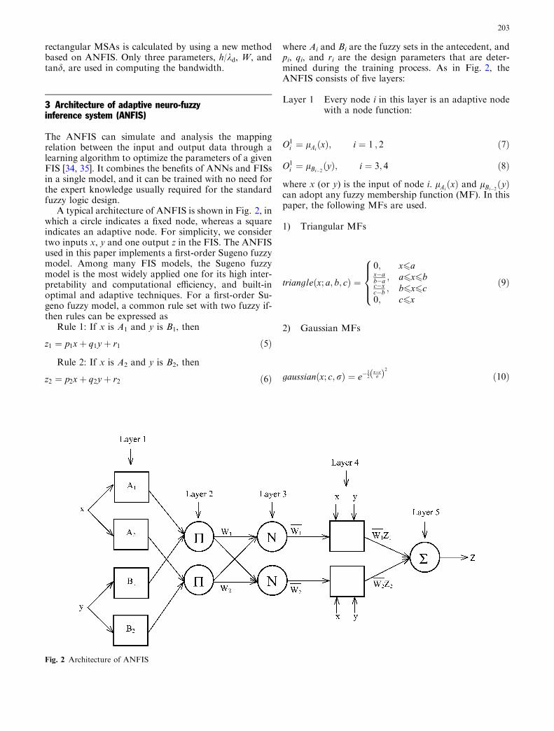
A typical architecture of ANFIS is shown in Fig. 2, inwhich a circle indicates a fixed node, whereas a squareindicates an adaptive node. For simplicity, we considertwo inputs x, y and one output z in the FIS. The ANFISused in this paper implements a first-order Sugeno fuzzymodel. Among many FIS models, the Sugeno fuzzymodel is the most widely applied one for its high inter-pretability and computational efficiency, and built-inoptimal and adaptive techniques. For a first-order Su-geno fuzzy model, a common rule set with two fuzzy if-then rules can be expressed as

Rule 1: If x is A1 and y is B1, then

z1 ¼ p1xþ q1y þ r1 ð5Þ

Rule 2: If x is A2 and y is B2, then

z2 ¼ p2xþ q2y þ r2 ð6Þ

where Ai and Bi are the fuzzy sets in the antecedent, andpi, qi, and ri are the design parameters that are deter-mined during the training process. As in Fig. 2, theANFIS consists of five layers:

Layer 1 Every node i in this layer is an adaptive nodewith a node function:

O1i ¼ lAi

ðxÞ; i ¼ 1 ; 2 ð7Þ

O1i ¼ lBi�2ðyÞ; i ¼ 3; 4 ð8Þ

where x (or y) is the input of node i. lAixð Þ and lBi�2 yð Þ

can adopt any fuzzy membership function (MF). In thispaper, the following MFs are used.

1) Triangular MFs

triangle x; a; b; cð Þ ¼

0; x6ax�ab�a ; a6x6bc�xc�b ; b6x6c0; c6x

8

>><

>>:

ð9Þ

2) Gaussian MFs

gaussian x; c; rð Þ ¼ e�12

x�crð Þ

2

ð10Þ

Fig. 2 Architecture of ANFIS

203

3) Trapezoidal MFs

trapezoid x; a; b; c; dð Þ ¼

0; x6ax�ab�a ; a6x6b

1; b6x6cd�xd�c ; c6x6d

0; d6x

8

>>>>>><

>>>>>>:

ð11Þ

where {ai, bi, ci, di, ri} is the parameter set that changesthe shapes of the MF. Parameters in this layer arenamed as the premise parameters.Layer 2 Every node in the second layer represents the

firing strength of a rule by multiplying theincoming signals and forwarding the productas:

O2i ¼ xi ¼ lAi

xð ÞlBiyð Þ; i ¼ 1 ; 2 ð12Þ

Layer 3 The ith node in this layer calculates the ratioof the ith rule’s firing strength to the sum ofall rules’ firing strengths:

O3i ¼ xi ¼

xi

x1 þ x2; i ¼ 1; 2 ð13Þ

where xi is referred to as the normalized firing strengths.Layer 4 The node function in this layer is represented

by

O4i ¼ xizi ¼ xi pixþ qiy þ rið Þ; i ¼ 1; 2 ð14Þ

where xi is the output of layer 3, and {pi, qi, ri} is theparameter set. Parameters in this layer are referred to asthe consequent parameters.Layer 5 The single node in this layer computes the

overall output as the summation of allincoming signals, which is expressed as:

O51 ¼

X2

i¼1xizi ¼

x1z1 þ x2z2x1 þ x2

ð15Þ

It is seen from the ANFIS architecture that when thevalues of the premise parameters are fixed, the overalloutput can be expressed as a linear combination of theconsequent parameters:

z ¼ x1xð Þp1 þ x1yð Þq1 þ x1ð Þr1 þ x2xð Þp2 þ x2yð Þq2

þ x2ð Þr2 ð16Þ

The least square method (LSM) can be used to findthe optimal values of the consequent parameters. When

the premise parameters are not fixed, the search spacebecomes larger and the convergence of training becomesslower. The hybrid learning algorithm [34, 35] combin-ing the LSM and the backpropagation (BP) algorithmcan be used to solve this problem. This algorithm con-verges much faster since it reduces the dimension of thesearch space of the BP algorithm. During the learningprocess, the premise parameters in layer 1 and the con-sequent parameters in layer 4 are tuned until the desiredresponse of the FIS is achieved. The hybrid learningalgorithm has a two-step process. First, while holdingthe premise parameters fixed, the functional signals arepropagated forward to layer 4, where the consequentparameters are identified by the LSM. Then, the con-sequent parameters are held fixed while the error signals,the derivative of the error measure with respect to eachnode output, are propagated from the output end to theinput end, and the premise parameters are updated bythe standard BP algorithm.

3.1 Application of ANFIS to the calculationof bandwidth

In this work, the ANFIS was used to compute thebandwidth of electrically thin and thick rectangularMSAs. For the ANFIS, the inputs are h/kd,W, and tand,and the output is the measured bandwidths BWme. TheANFIS model used for computing the bandwidth isillustrated in Fig. 3.

There are two types of data generators for antennaapplications. These data generators are the measurementand simulation. The selection of a data generator de-pends on the application and the availability of the datagenerator. The training and test data sets used in thispaper have been obtained from previous experimentalworks [28, 29], and are given in Table 1. The 27 data setsin Table 1 were used to train the ANFIS. The 6 datasets, marked with an asterisk in Table 1, were used fortesting. The training and test data sets used in this paperare also the same as those used for ANNs [30, 32] andFISs [31]. The antennas given in Table 1 vary in elec-trical thickness from 0.0065 to 0.2284, and in physicalthickness from 0.17 to 12.81 mm, and operate over thefrequency range 2.980–8.000 GHz.

Fig. 3 ANFIS model for bandwidth calculation

204

Training an ANFIS with the use of the hybridlearning algorithm to calculate the bandwidth involvespresenting it sequentially with different sets (h/kd, W,tand) and corresponding measured values BWme. Dif-ferences between the target output BWme and the actualoutput of the ANFIS are evaluated by the hybridlearning algorithm. The adaptation is carried out afterthe presentation of each set (h/kd, W, tand) until thecalculation accuracy of the ANFIS is deemed satisfac-tory according to some criterion (for example, when theerror between BWme and the actual output for allthe training set falls below a given threshold) or whenthe maximum allowable number of epochs is reached.

The number of epoch was 700 for training. Thenumber of membership functions for the input variablesh/kd, W, and tand are 4, 3, and 2, respectively. Thenumber of rules is then 24 (4·3·2=24). The MFs for theinput variables h/kd, W, and tand are the triangular,gaussian, and trapezoidal, respectively. It is clear fromEqs. (9), (10) and (11) that the triangular, gaussian, andtrapezoidal MFs are specified by 3, 2, and 4 parameters,respectively. Therefore, the ANFIS used here contains atotal of 122 fitting parameters, of which 26

(4·3+3·2+2·4=26) are the premise parameters and 96(4·24=96) are the consequent parameters.

4 Results and conclusions

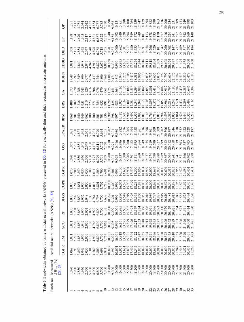
The bandwidths calculated by using ANFIS proposed inthis paper for electrically thin and thick rectangularmicrostrip patch antennas are listed in Table 1. Forcomparison, the results obtained by using the conven-tional methods [1, 16, 26, 27, 29, 33], by using ANNs [30,32], and by using FISs [31] are given in Tables 2, 3, and4, respectively. CGFR, LM, SCG, RP, BFGS, CGPB,CGPR, BR, OSS, BPALR, BPM, DRS, GA, RBFN,EDBD, DBD, BP, and QP in Table 3 represent,respectively, the bandwidths calculated by using ANNs[32] trained by conjugate gradient of Fletcher-Reeves(CGFR), Levenberg-Marquardt (LM), scaled conjugategradient (SCG), resilient backpropagation (RP), Broy-den-Fletcher-Goldfarb-Shanno (BFGS), conjugate gra-dient of Powell-Beale (CGPB), conjugate gradient ofPolak-Ribiere (CGPR), bayesian regularization (BR),one-step secant (OSS), backpropagation with adaptive

Table 1 The measured bandwidths and the bandwidths obtained from the ANFIS proposed in this paper for electrically thin and thickrectangular microstrip antennas

Patch no h(mm)

fr (GHz) h/kd W(mm)

tand Measured [28, 29]BWme (%)

Present ANFIS method

1 0.17 7.740 0.0065 8.50 0.001 1.070 1.0702 0.79 3.970 0.0155 20.00 0.001 2.200 2.2003 0.79 7.730 0.0326 10.63 0.001 3.850 3.8504 0.79 3.545 0.0149 20.74 0.002 1.950 1.9505 1.27 4.600 0.0622 9.10 0.001 2.050 2.0506 1.57 5.060 0.0404 17.20 0.001 5.100 5.1007* 1.57 4.805 0.0384 18.10 0.001 4.900 4.9268 1.63 6.560 0.0569 12.70 0.002 6.800 6.8009 1.63 5.600 0.0486 15.00 0.002 5.700 5.70010* 2.00 6.200 0.0660 13.37 0.002 7.700 7.71611 2.42 7.050 0.0908 11.20 0.002 10.900 10.90012 2.52 5.800 0.0778 14.03 0.002 9.300 9.30013 3.00 5.270 0.0833 15.30 0.002 10.000 10.00014* 3.00 7.990 0.1263 9.05 0.002 16.000 16.05915 3.00 6.570 0.1039 11.70 0.002 13.600 13.60016 4.76 5.100 0.1292 13.75 0.002 15.900 15.90017 3.30 8.000 0.1405 7.76 0.002 17.500 17.50018* 4.00 7.134 0.1519 7.90 0.002 18.200 18.30419 4.50 6.070 0.1454 9.87 0.002 17.900 17.90020 4.76 5.820 0.1475 10.00 0.002 18.000 18.00021 4.76 6.380 0.1617 8.14 0.002 19.000 19.00022 5.50 5.990 0.1754 7.90 0.002 20.000 20.00023 6.26 4.660 0.1553 12.00 0.002 18.700 18.70024 8.54 4.600 0.2091 7.83 0.002 20.900 20.90025 9.52 3.580 0.1814 12.56 0.002 20.000 20.00026 9.52 3.980 0.2017 9.74 0.002 20.600 20.60027* 9.52 3.900 0.1976 10.20 0.002 20.300 20.30728 10.00 3.980 0.2119 8.83 0.002 20.900 20.90029 11.00 3.900 0.2284 7.77 0.002 21.960 21.96030 12.00 3.470 0.2216 9.20 0.002 21.500 21.50031 12.81 3.200 0.2182 10.30 0.002 21.600 21.60032 12.81 2.980 0.2032 12.65 0.002 20.400 20.40033* 12.81 3.150 0.2148 10.80 0.002 21.200 21.183

*Test data sets

205

learning rate (BPALR), backpropagation with momen-tum (BPM), directed random search (DRS), and geneticalgorithms (GA), and the bandwidths calculated byusing the radial basis function network (RBFN) [32]trained by extended delta-bar-delta algorithm (EDBD),and the bandwidths calculated by using ANNs [30]trained by EDBD, delta-bar-delta (DBD), backpropa-gation (BP), and quick propagation (QP) algorithms.The entries of ITSA, MTSA, and CTSA in Table 4represent, respectively, the bandwidths calculated byusing FISs [31] trained by improved tabu search algo-rithm (ITSA), modified tabu search algorithm (MTSA),and classical tabu search algorithm (CTSA). The sum ofthe absolute errors between the theoretical and experi-mental results in Tables 1, 2, 3, and 4 for every methodis also listed in Table 5.

As it is seen from Table 2, the conventional methodsgive comparable results—some cases are in goodagreement with measurements, and others are far off.The bandwidth results of [16] were obtained by thestandard cavity model programmed by Pozar [54] in hisMSAnt program. This program is only valid for elec-trically thin MSAs. The method in [1] is found to yieldbandwidths of MSAs with substrates thinner than

approximately 0.17kd with reasonable accuracy; how-ever, it becomes increasingly inaccurate as the substratethickness increases. The results of an approximatebandwidth formula [26] based on a rigorous Sommerfeldsolution are not in good agreement with the measuredresults. The closed-form expression, based on the mod-ified cavity model and the exact Green’s function for agrounded dielectric slab, was proposed by Kara [29] forcomputing the bandwidth of electrically thick rectan-gular MSAs. To closely fit the measured bandwidth re-sults, the correction factor derived by means of a curve-fitting technique was also included in the closed-formexpression [29]. The results of this closed-form expres-sion are close to the experimental results only forelectrically thick configurations; as shown in Table 2.The results of Guney [27] were obtained from the curve-fitting expression based on the results of Green’s func-tion methods. It was shown by Guney [27] that theresults of the curve-fitting expression are in goodagreement with the results of moment method approach[18] and electric surface current model [21]. However, itis evident from Table 2 that the results of the curve-fitting expression are not in good agreement with themeasured results. Guney [33] also proposed a very

Table 2 Bandwidths obtained from conventional methods available in the literature [1, 16, 26, 27, 29, 33] for electrically thin and thickrectangular microstrip antennas

Patch no Measured BWme (%)[28, 29]

Conventional methods in the literature

[16] [1] [26] [29] [27] [33]

1 1.070 0.82 0.84 0.30 1.20 0.26 3.132 2.200 1.45 2.03 0.87 2.78 0.75 5.343 3.850 2.99 3.76 1.88 5.03 1.64 7.514 1.950 1.29 1.69 0.72 2.46 0.61 4.645 2.050 1.54 1.90 0.72 4.09 0.84 3.966 5.100 4.21 5.14 2.67 6.46 2.35 9.217 4.900 3.96 4.87 2.51 6.17 2.20 8.938 6.800 5.98 6.70 3.69 8.12 3.43 10.569 5.700 4.76 5.69 3.02 7.12 2.78 9.6110 7.700 7.29 7.81 4.41 9.16 4.20 11.5711 10.900 11.31 10.88 6.39 11.72 6.50 13.9912 9.300 9.14 9.26 5.36 10.42 5.26 12.7713 10.000 10.30 10.14 5.88 11.15 5.83 13.4714 16.000 18.42 15.64 9.41 15.16 10.36 17.2315 13.600 13.84 12.75 7.53 13.14 7.90 15.3616 15.900 18.06 15.73 9.35 15.11 10.50 17.1617 17.500 15.29 18.48 8.39 17.00 11.28 17.6418 18.200 13.62 20.09 8.15 17.77 12.18 18.2019 17.900 14.54 19.17 8.31 17.34 11.70 17.9120 18.000 14.08 19.46 8.19 17.47 11.80 17.9621 19.000 12.45 21.47 7.95 18.42 12.93 18.6822 20.000 10.73 23.41 7.63 19.29 14.10 19.4123 18.700 13.01 20.55 8.10 18.01 12.57 18.4624 20.900 7.85 28.24 6.76 21.26 16.49 20.9325 20.000 10.10 24.27 7.46 19.66 14.54 19.6826 20.600 8.45 27.17 7.02 20.85 16.10 20.6627 20.300 8.76 26.59 7.10 20.61 15.76 20.4528 20.900 7.63 28.64 6.67 21.40 16.65 21.0429 21.960 6.50 31.03 6.14 22.26 17.56 21.6930 21.500 6.92 30.06 6.32 21.91 17.13 21.3931 21.600 7.11 29.56 6.41 21.73 16.95 21.2632 20.400 8.26 27.39 6.90 20.92 16.07 20.6633 21.200 7.39 29.07 6.54 21.55 16.77 21.13

206

Table

3Bandwidthsobtained

byusingartificialneuralnetworks(A

NNs)

presentedin

[30,32]forelectricallythin

andthickrectangularmicrostripantennas

Patchno

Measured

BW

me(%

)[28,29]

Artificialneuralnetworks(A

NNs)

[30,32]

CGFR

LM

SCG

RP

BFGS

CGPB

CGPR

BR

OSS

BPALR

BPM

DRS

GA

RBFN

EDBD

DBD

BP

QP

11.070

1.069

1.071

1.071

1.070

1.070

1.070

1.070

1.070

1.067

1.071

1.068

1.400

1.573

1.048

1.081

1.068

1.178

1.271

22.200

2.199

2.200

2.200

2.201

2.202

2.200

2.200

2.200

2.203

2.200

2.201

2.182

2.620

2.292

2.193

2.197

2.304

2.117

33.850

3.850

3.850

3.850

3.850

3.850

3.851

3.850

3.850

3.853

3.837

3.840

3.336

3.288

3.849

3.840

3.854

3.670

3.753

41.950

1.949

1.950

1.949

1.950

1.952

1.950

1.950

1.950

1.948

1.945

1.949

1.951

1.943

1.899

1.948

1.948

1.905

2.034

52.050

2.050

2.050

2.050

2.051

2.048

2.050

2.050

2.050

2.049

2.061

2.062

2.210

2.120

2.077

2.046

2.047

2.117

2.612

65.100

5.101

5.100

5.100

5.099

5.100

5.099

5.100

5.100

5.100

5.097

5.100

5.223

4.816

5.024

4.945

5.340

5.211

4.837

74.900

4.560

4.900

4.766

4.922

4.764

4.016

4.011

5.175

4.137

4.233

4.300

4.571

4.506

4.437

4.916

4.898

4.831

4.854

86.800

6.800

6.800

6.800

6.800

6.798

6.801

6.800

6.799

6.811

6.790

6.801

6.754

7.076

6.744

6.824

6.788

6.887

6.757

95.700

5.699

5.700

5.700

5.700

5.700

5.702

5.700

5.701

5.702

5.694

5.701

5.632

5.470

5.806

5.679

5.718

5.822

5.783

10

7.700

7.811

7.763

7.862

8.132

7.639

7.719

7.691

7.869

7.760

7.705

7.536

7.891

8.061

7.968

8.006

7.865

7.727

7.730

11

10.900

10.899

10.901

10.903

10.900

10.926

10.900

10.900

10.900

10.910

10.902

10.906

11.285

11.250

11.080

10.858

10.901

11.040

10.998

12

9.300

9.299

9.299

9.305

9.299

9.301

9.300

9.301

9.302

9.271

9.301

9.298

9.425

9.451

9.471

9.336

9.287

9.155

9.085

13

10.000

10.001

10.001

9.999

10.001

9.999

9.999

9.999

9.998

10.016

9.980

9.997

9.983

9.864

9.813

9.990

10.000

10.092

10.131

14

16.000

15.954

15.918

16.161

15.995

15.890

16.063

16.100

16.337

16.396

15.982

16.182

15.924

16.167

15.940

15.975

15.862

15.940

15.851

15

13.600

13.601

13.599

13.595

13.605

13.548

13.598

13.600

13.600

13.598

13.576

13.593

13.169

13.135

13.225

13.607

13.601

13.528

13.388

16

15.900

15.899

15.901

15.899

15.902

15.919

15.902

15.901

15.905

15.900

15.905

15.906

16.003

16.086

16.106

15.881

15.917

15.994

16.100

17

17.500

17.499

17.504

17.496

17.493

17.496

17.499

17.502

17.501

17.482

17.494

17.499

17.284

17.516

17.417

17.523

17.480

17.349

17.264

18

18.200

18.345

18.422

18.217

18.179

18.365

18.297

18.300

18.311

18.395

18.458

18.537

18.340

18.394

18.381

18.254

18.433

18.372

18.339

19

17.900

17.877

17.847

17.853

17.824

17.850

17.871

17.869

17.860

17.864

17.861

17.890

17.947

17.883

17.996

17.844

17.917

17.949

17.947

20

18.000

18.023

18.055

18.048

18.066

18.051

18.035

18.034

18.019

18.049

18.036

18.010

18.129

18.046

18.170

18.016

18.091

18.101

18.129

21

19.000

19.004

19.004

19.013

19.026

19.016

18.999

18.999

19.037

19.055

19.098

19.146

19.103

19.050

19.035

19.113

19.054

19.113

19.094

22

20.000

20.000

19.991

19.998

19.991

19.989

20.000

20.000

19.974

19.919

19.801

19.764

19.893

19.801

19.733

19.818

19.766

19.878

19.883

23

18.700

18.699

18.696

18.695

18.696

18.797

18.698

18.697

18.699

18.690

18.709

18.719

18.572

18.419

18.655

18.804

18.620

18.433

18.599

24

20.900

20.919

20.897

20.897

20.893

20.887

20.903

20.906

20.888

20.927

21.009

21.016

21.135

21.136

21.076

21.009

21.101

21.170

21.163

25

20.000

20.000

20.000

20.005

20.000

19.819

20.002

20.000

19.989

19.999

19.902

19.902

19.859

19.807

19.792

19.851

19.842

19.857

19.836

26

20.600

20.600

20.592

20.606

20.579

20.610

20.596

20.604

20.667

20.612

20.596

20.593

20.969

20.917

20.797

20.608

20.760

20.916

20.900

27

20.300

20.237

20.455

20.562

20.429

20.484

20.505

20.517

20.604

20.512

20.397

20.382

20.818

20.796

20.638

20.524

20.608

20.724

20.734

28

20.900

20.873

20.910

20.889

20.921

20.913

20.891

20.883

20.841

20.958

21.046

21.033

21.247

21.190

21.175

20.977

21.147

21.241

21.231

29

21.960

21.948

21.953

21.963

21.934

21.941

21.952

21.955

21.941

21.939

21.818

21.861

21.521

21.702

21.782

21.885

21.777

21.557

21.609

30

21.500

21.545

21.520

21.506

21.573

21.583

21.522

21.523

21.571

21.503

21.552

21.526

21.439

21.435

21.513

21.495

21.469

21.412

21.433

31

21.600

21.571

21.590

21.596

21.541

21.525

21.591

21.589

21.566

21.557

21.422

21.444

21.298

21.385

21.339

21.535

21.317

21.342

21.249

32

20.400

20.405

20.401

20.400

20.414

20.494

20.401

20.401

20.402

20.403

20.528

20.520

20.499

20.646

20.479

20.500

20.592

20.569

20.498

33

21.200

21.265

21.493

21.481

21.370

21.270

21.431

21.431

21.279

21.407

21.197

21.218

21.166

21.309

21.180

21.460

21.184

21.148

21.103

207

simple bandwidth expression based on the experimentalresults for MSAs with thick substrates. As the thicknessof the substrate decreases, the accuracy of this simpleexpression decreases rapidly.

It can be seen from Tables 2, 3, 4, and 5 that theresults of all neural models and fuzzy inference systemsare better than those predicted by the conventionalmethods. These results clearly show the superiority ofartificial intelligence techniques over the conventionalmethods. When the performances of neural modelspresented in [30, 32] are compared with each other, thehighest accuracy was achieved with the ANN trained byCGFR algorithm. The best result for FISs [31] is ob-tained from the FIS trained by ITSA.

We observe that the results of ANFIS show betteragreement with the experimental results as comparedto the results of the conventional methods [1, 16, 26,27, 29, 33], ANNs [30, 32], and FISs [31]. This is clearfrom Tables 1, 2, 3, 4, and 5. The very good agree-ment between the experimental results and our com-puted bandwidth results supports the validity of theANFIS model presented in this paper. A prominentadvantage of the ANFIS model is that, after proper

training, ANFIS completely bypasses the repeated useof complex iterative processes for new cases presentedto it.

In this paper, the ANFIS is trained and tested withthe experimental data taken from the previous experi-mental works [28, 29]. It is clear from Tables 2 and 5that the theoretical bandwidth results of the conven-tional methods are not in very good agreement with theexperimental results. For this reason, the theoreticaldata sets obtained from the conventional methods arenot used in this work. Only the measured data set is usedfor training and testing the ANFIS. It also needs to beemphasized that better results may be obtained from theANFIS either by choosing different training and testdata sets from the ones used in the paper or by supplyingmore input data set values for training.

As a result, the ANFIS trained by means of themeasured data is presented to calculate accurately thebandwidth of electrically thin and thick rectangularMSAs with substrates satisfying 0.0065 £ h/kd £ 0.2284and 0.17 mm £ h £ 12.81 mm. The hybrid learningalgorithm is used to optimize the parameters of ANFIS.In this algorithm, the parameters defining the shape of

Table 4 Bandwidths obtained by using fuzzy inference systems(FISs) presented in [31] for electrically thin and thick rectangularmicrostrip antennas

Patch no MeasuredBWme

(%)[28, 29]Fuzzy inferencesystems (FISs) [31]

ITSA MTSA CTSA

1 1.070 1.070 1.070 1.0702 2.200 2.200 2.200 2.2003 3.850 3.848 3.850 3.8504 1.950 1.950 1.950 1.9595 2.050 2.051 2.050 2.0506 5.100 5.101 5.100 5.1007 4.900 4.899 4.895 4.9008 6.800 6.775 6.798 6.5959 5.700 5.699 5.711 5.67610 7.700 7.759 7.769 7.87711 10.900 10.906 10.896 11.21712 9.300 9.255 9.287 9.47613 10.000 10.003 9.994 9.86014 16.000 16.005 16.139 15.99815 13.600 13.598 13.600 13.17416 15.900 15.914 15.905 16.05017 17.500 17.450 17.324 17.44218 18.200 18.288 18.284 18.35719 17.900 17.845 17.797 17.88420 18.000 18.060 17.977 18.05021 19.000 18.955 19.110 18.98822 20.000 19.999 19.955 19.71423 18.700 18.690 18.688 18.60324 20.900 20.896 20.917 21.08025 20.000 19.997 20.035 19.79026 20.600 20.602 20.478 20.75927 20.300 20.296 20.274 20.59928 20.900 20.909 21.056 21.14529 21.960 21.960 21.973 21.74130 21.500 21.510 21.580 21.46131 21.600 21.566 21.377 21.30932 20.400 20.401 20.514 20.52633 21.200 21.221 21.173 21.178

Table 5 Sum of absolute errors between measured and calculatedbandwidths

Methods Total absolutedeviationsfrom the measureddata (%)

ANFIS Present method 0.229

Conventionalmethods in theliterature

[16] 178.69

[1] 88.76[26] 266.93[29] 23.92[27] 140.02[33] 50.51

Artificial neuralnetworks (ANNs)[30, 32]

CGFR 0.969

LM 1.009SCG 1.191RP 1.200BFGS 1.550CGPB 1.635CGPR 1.687BR 1.685OSS 2.332BPALR 2.393BPM 2.612DRS 6.332GA 7.790RBFN 4.963EDBD 2.315DBD 3.129BP 4.962QP 5.816

Fuzzy Inferencesystems (FISs)[31]

ITSA 0.562

MTSA 1.620CTSA 4.092

208

the MFs are identified by the BP algorithm while theconsequent parameters are identified by the LSM. Theresults of ANFIS are in excellent agreement withthe measurements, and better accuracy with respect tothe previous conventional and artificial intelligencetechniques is obtained. The ANFIS has the advantagesof easy implementation and good learning ability. Itmust also be emphasized that the proposed method isnot limited to the bandwidth calculation of rectangularMSAs. This method can easily be applied to other an-tenna and microwave circuit problems. Accurate, fast,and reliable ANFIS models can be developed frommeasured/simulated antenna data. Once developed,these ANFIS models can be used in place of computa-tionally intensive numerical models to speed up antennadesign.

References

1. Bahl IJ, Bhartia P (1980) Microstrip antennas. Artech House,Canton, MA

2. James JR, Hall PS, Wood C (1981) Microstrip antennas-theoryand design. Peregrinus, London

3. Gupta KC, Benalla A (1988) Microstrip antenna design. ArtechHouse, Canton, MA

4. James JR, Hall PS (1989) Handbook of microstrip antennas.IEE Electromagnetic wave series, Peregrinus, London, 1–2(28):219–274

5. Bhartia P, Rao KVS, Tomar RS (1991) Millimeter-wave mi-crostrip and printed circuit antennas. Artech House, Canton,MA

6. Hirasawa K, Haneishi M (1992) Analysis, design, and mea-surement of small and low-profile antennas. Artech House,Canton, MA

7. Pozar DM, Schaubert DH (1995) Microstrip antennas-theanalysis and design of microstrip antennas and arrays. IEEEPress, New York

8. Zurcher JF, Gardiol FE (1995) Broadband patch antennas.Artech House, Canton, MA

9. Sainati RA (1996) CAD of microstrip antennas for wirelessapplications. Artech House, Canton, MA

10. Lee KF, Chen W (1997) Advances in microstrip and printedantennas. Wiley, New York

11. Wong KL (1999) Design of nonplanar microstrip antennas andtransmission lines. Wiley, New York

12. Garg R, Bhartia P, Bahl I, Ittipiboon A (2001) Microstripantenna design handbook. Artech House, Canton, MA

13. Wong KL (2001) Compact and broadband microstrip anten-nas. Wiley, New York

14. Vandensande J, Pues H, Van De Capelle A (1979) Calculationof the bandwidth of microstrip resonator antennas. In: Pro-ceedings of 9th European microwave conference, Brighton,England, pp 116–119

15. Derneryd AG, Lind AG (1979) Extended analysis of rectan-gular microstrip resonator antenna. IEEE Trans AntennasPropagat 27:846–849

16. Carver KR, Mink JW (1981) Microstrip antenna technology.IEEE Trans Antennas Propagat 29:2–24

17. Richards WF, Lo YT, Harrison DD (1981) An improved the-ory for microstrip antennas and applications. IEEE TransAntennas Propagat 29:38–46

18. Pozar DM (1983) Considerations for millimeter wave printedantennas. IEEE Trans Antennas Propagat 31:740–747

19. Kumar G, Gupta KC (1984) Broadband microstrip antennasusing additional resonators gap coupled to the radiating edges.IEEE Trans Antennas Propagat 32:1375–1379

20. Pues HF, Van De Capelle AR (1984) Accurate transmission-line model for the rectangular microstrip antennas. In: ProcIEE Microw Antennas Propagat H 13:334–340

21. Perlmutter P, Shtrikman S, Treves D (1985) Electric surfacecurrent model for the analysis of microstrip antennas withapplication to rectangular elements. IEEE Trans AntennasPropagat 33:301–311

22. Bhattacharyya K, Garg R (1986) Effect of substrate on theefficiency of an arbitrarily shaped microstrip patch antenna.IEEE Trans Antennas Propagat 34:1181–1188

23. Chang E, Long SA, Richards WF (1986) An experimentalinvestigation of electrically thick rectangular microstripantennas. IEEE Trans Antennas Propagat 34:767–772

24. Pozar DM, Voda SM (1987) A rigorous analysis of a microstripline fed patch antenna. IEEE Trans Antennas Propagat35:1343–1350

25. Pues HF, Van De Capelle AR (1989) An impedance matchingtechnique for increasing the bandwidth of microstrip antennas.IEEE Trans Antennas Propagat 37:1345–1354

26. Jackson DR, Alexopoulos NG (1991) Simple approximateformulas for input resistance, bandwidth, and efficiency of aresonant rectangular patch. IEEE Trans Antennas Propagat39:407–410

27. Guney K (1994) Bandwidth of a resonant rectangular micro-strip antenna. Microw Opt Technol Lett 7:521–524

28. Kara M (1996) A simple technique for the calculation ofbandwidth of rectangular microstrip antenna elements withvarious substrate thicknesses. Microw Opt Technol Lett 12:16–20

29. Kara M (1996) A novel technique to calculate the bandwidth ofrectangular microstrip antenna elements with thick substrates.Microw Opt Technol Lett 12:59–64

30. Sagiroglu S, Guney K, Erler M (1999) Calculation of band-width for electrically thin and thick rectangular microstripantennas with the use of multilayered perceptrons. Int J Mi-crow Comput Aided Eng 9:277–286

31. Kaplan A, Guney K, Ozer S (2001) Fuzzy associative memoriesfor the computation of the bandwidth of rectangular microstripantennas with thin and thick substrates. Int J Electron 88:189–195

32. Gultekin S, Guney K, Sagiroglu S (2003) Neural networks forthe calculation of bandwidth of rectangular microstrip anten-nas. Appl Comput Electromagn Soc J 18:46–56

33. Guney K (2003) A simple and accurate expression for thebandwidth of electrically thick rectangular microstrip antennas.Microw Opt Technol Lett 36:225–228

34. Jang J-SR (1993) ANFIS: Adaptive-network-based fuzzyinference system. IEEE Trans Syst Man Cybern 23:665–685

35. Jang J-SR, Sun CT, Mizutani E (1997) Neuro-fuzzy and softcomputing: A computational approach to learning and ma-chine intelligence. Prentice-Hall, Englewood Cliffs, NJ

36. Brown M, Haris C (1994) Neurofuzzy adaptive modeling andcontrol. Prentice-Hall, Englewood Cliffs, NJ

37. Constantin VA (1995) Fuzzy logic and neuro-fuzzy applica-tions explained. Prentice-Hall, Englewood Cliffs, NJ

38. Lin CT, Lee CSG (1996) Neural fuzzy systems: A neuro-fuzzysynergism to intelligent systems. Prentice-Hall, EnglewoodCliffs, NJ

39. Kim J, Kasabov N (1999) HyFIS: Adaptive neuro-fuzzyinference systems and their application to nonlinear dynamicalsystems. Neural Netw 12:1301–1319

40. Guney K, Sarikaya N (2004) Adaptive neuro-fuzzy inferencesystem for the input resistance computation of rectangularmicrostrip antennas with thin and thick substrates. J Electro-magn Waves Appl 18:23–39

41. Guney K, Sarikaya N (2004) Computation of resonant fre-quency for equilateral triangular microstrip antennas with theuse of adaptive neuro-fuzzy inference system. Int J MicrowComput Aided Eng (in press)

42. Guney K, Sarikaya N (2004) Input resistance calculation forcircular microstrip antennas using adaptive neuro-fuzzy infer-ence system. Int J Infrared Millimeter Waves (in press)

209

43. Ozer S, Guney K, Kaplan A (2000) Computation of the reso-nant frequency of electrically thin and thick rectangular mi-crostrip antennas with the use of fuzzy inference systems. Int JMicrow Comput Aided Eng 10:108–119

44. Sagiroglu S, Guney K (1997) Calculation of resonant frequencyfor an equilateral triangular microstrip antenna with the use ofartificial neural networks. Microw Opt Technol Lett 14:89–93

45. Sagiroglu S, Guney K, Erler M (1998) Resonant frequencycalculation for circular microstrip antennas using artificialneural networks. Int J Microw Comput Aided Eng 8:270–277

46. Karaboga D, Guney K, Sagiroglu S, Erler M (1999) Neuralcomputation of resonant frequency of electrically thin andthick rectangular microstrip antennas. In: Proc IEE MicrowAntennas Propagat H 146:155–159

47. Guney K, Erler M, Sagiroglu S (2000) Artificial neural net-works for the resonant resistance calculation of electrically thinand thick rectangular microstrip antennas. Electromagnetics20:387–400

48. Guney K, Sagiroglu S, Erler M (2001) Comparison of neuralnetworks for resonant frequency computation of electricallythin and thick rectangular microstrip antennas. J ElectromagnWaves Appl 15:1121–1145

49. Guney K, Sagiroglu S, Erler M (2002) Design of rectangularmicrostrip antennas with the use of artificial neural networks.Neural Netw World 4:361–370

50. Guney K, Sagiroglu S, Erler M (2002) Generalized neuralmethod to determine resonant frequencies of various microstripantennas. Int J Microw Comput Aided Eng 12:131–139

51. Yildiz C, Gultekin SS, Guney K, Sagiroglu S (2002) Neuralmodels for the resonant frequency of electrically thin and thickcircular microstrip antennas and the characteristic parametersof asymmetric coplanar waveguides backed with a conductor.AEU Int J Electron Commun 56:396–406

52. Guney K, Sarikaya N (2003) Artificial neural networks forcalculating the input resistance of circular microstrip antennas.Microw Opt Technol Lett 37:107–111

53. Guney K, Sarikaya N (2004) Artificial neural networks for thenarrow aperture dimension calculation of optimum gainpyramidal horns. Electr Eng 86:157–163

54. Pozar DM (1985) Antenna design using personal computers.Artech House, Canton, MA

210