adaptive cloud simulation using position based fluids charles welton ferreira barbosa yoshinori...
TRANSCRIPT

Adaptive Cloud Simulation Using Position Based Fluids
Charles Welton Ferreira BarbosaYoshinori Dobashi
Yamamoto Tsuyoshi
Hokkaido University
Overview
• Introduction• Related Work• Proposed Method• Results• Conclusion

Introduction
• Visual simulation of clouds– synthesizing images of outdoor scenes– flight simulators, movies, computer games, etc– procedural or physically-based approaches
[Dobashi00][Schpok 2003][Gardner 1985] [Miyazaki02]

Introduction
• Physically-based approach– realistic shapes and motions– simulation of atmospheric fluid dynamics– grid-based methods only
[Dobashi00][Schpok 2003][Gardner 1985] [Miyazaki02]
Our Goal
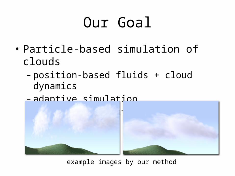
• Particle-based simulation of clouds– position-based fluids + cloud dynamics– adaptive simulation– efficient simulation using GPU
example images by our method

Overview
• Introduction• Related Work• Proposed Method• Results• Conclusion
Related Work
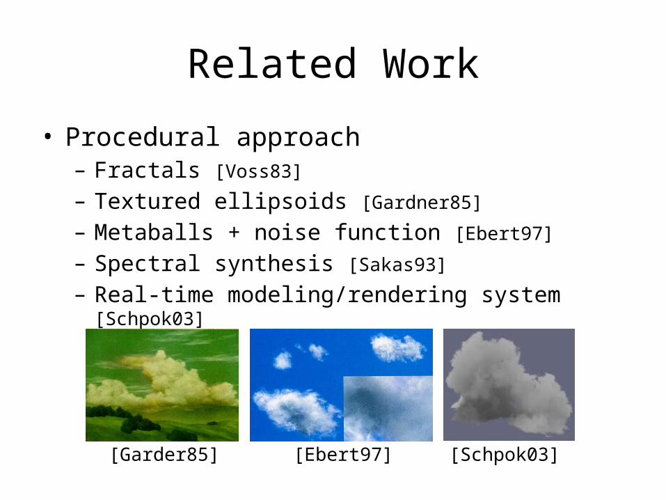
• Procedural approach– Fractals [Voss83]
– Textured ellipsoids [Gardner85]
– Metaballs + noise function [Ebert97]
– Spectral synthesis [Sakas93]
– Real-time modeling/rendering system [Schpok03]
[Garder85] [Ebert97] [Schpok03]

Related Work
• Physically-based approach– Numerical solution of atmospheric fluid dynamics
[Kajiya84, Miyazaki01, Miyazaki02, Dobashi08]
– No particle-based methods
[Miyazaki01] [Miyazaki02] [Dobashi08]

Related Work
• Particle-based methods for fluids– Smoothed particle hydrodynamics (SPH)
[Muller03, Solenthaler09, Ihmsen14]
– Position-based fluids (PBF) [Muller07, Macklin13, Macklin14]
• We use PBF for simulating clouds
[Cornelis14] [Macklin13]

Overview
• Introduction• Related Work• Proposed Method• Results• Conclusion

Proposed Method
• Overview of cloud formation process• Simulation method• Adaptive particles
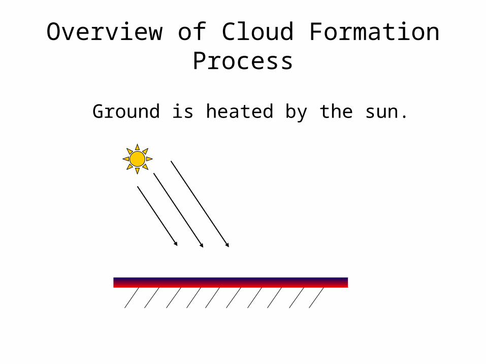
Overview of Cloud Formation Process
Ground is heated by the sun.
Overview of Cloud Formation Process
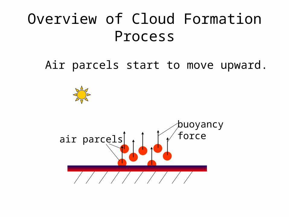
Air parcels start to move upward.
air parcels
buoyancyforce

Overview of Cloud Formation Process
Temperature of air parcels decreases.
adiabaticcooling

Overview of Cloud Formation Process
Clouds are generated due to phase transition
phase transition
(vapor cloud)

Overview of Cloud Formation Process
phase transition
latent heat is liberated due tophase transition
(vapor cloud)
Overview of Cloud Formation Process
phase transition
additional buoyancy
latent heat is liberated due tophase transition
(vapor cloud)

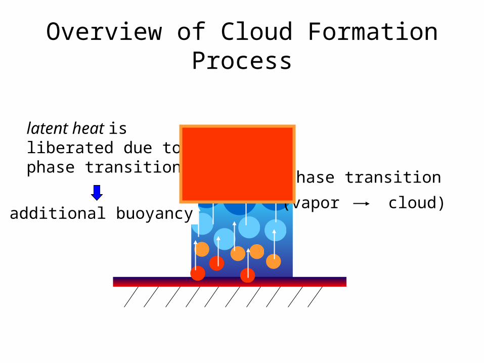
Overview of Cloud Formation Process
phase transition
additional buoyancy
further cloud growth
latent heat is liberated due tophase transition
(vapor cloud)
Proposed Method
• Overview of cloud formation process• Simulation method• Adaptive particles

Simulation Method
simulation space

Simulation Method
simulation space
(per
iodi
c bo
unda
ry) (periodic boundary)
boundary particles
boundary particles

Simulation Method
simulation space
• position, p• mass, m• velocity, (ux, uy)• temperature, T• vapor density, v• cloud density, w
position-based fluids
cloud formation
(per
iodi
c bo
unda
ry) (periodic boundary)
boundary particles
boundary particles

Simulation Method
• Processes during a single time step1. heat from the ground2. buoyancy force3. adiabatic cooling4. phase transition5. latent heat6. update particle positions with PBF

1. Heat from the Ground
• Increase temperature of particle i near ground:
ei Sdt
dT
temperature
time
temperature of external heat source
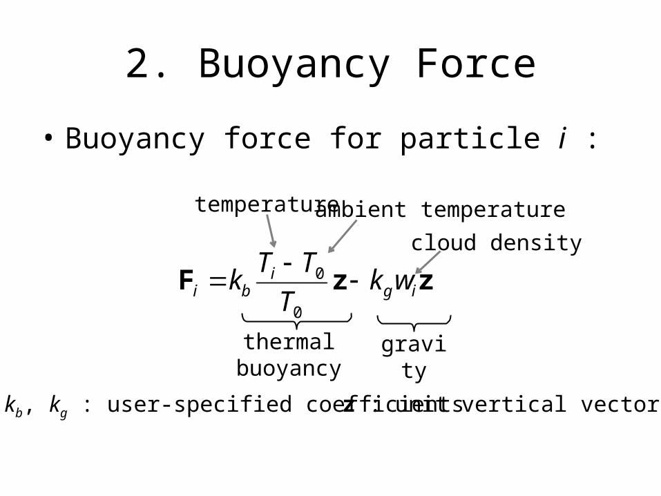
2. Buoyancy Force
• Buoyancy force for particle i :
zzF igi
bi wkT
TTk
0
0
temperature
cloud density
kb, kg : user-specified coefficients z : unit vertical vector
thermal buoyancy gravity
ambient temperature

3. Adiabatic Cooling
• Decrease temperature of particle i:
yi udt
dT
temperature
time
dry adiabatic lapse rate(user-specified)
vertical speed of particle i
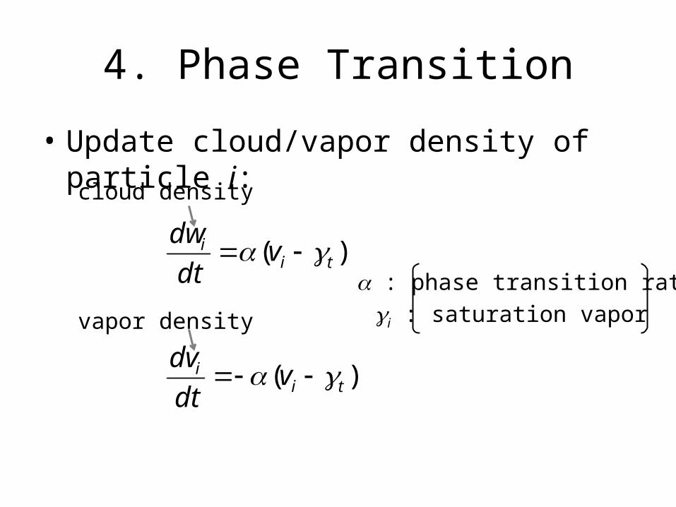
4. Phase Transition
• Update cloud/vapor density of particle i:
)( tii v
dt
dw
)( tii vdt
dv
cloud density
vapor density
a : phase transition rategi : saturation vapor
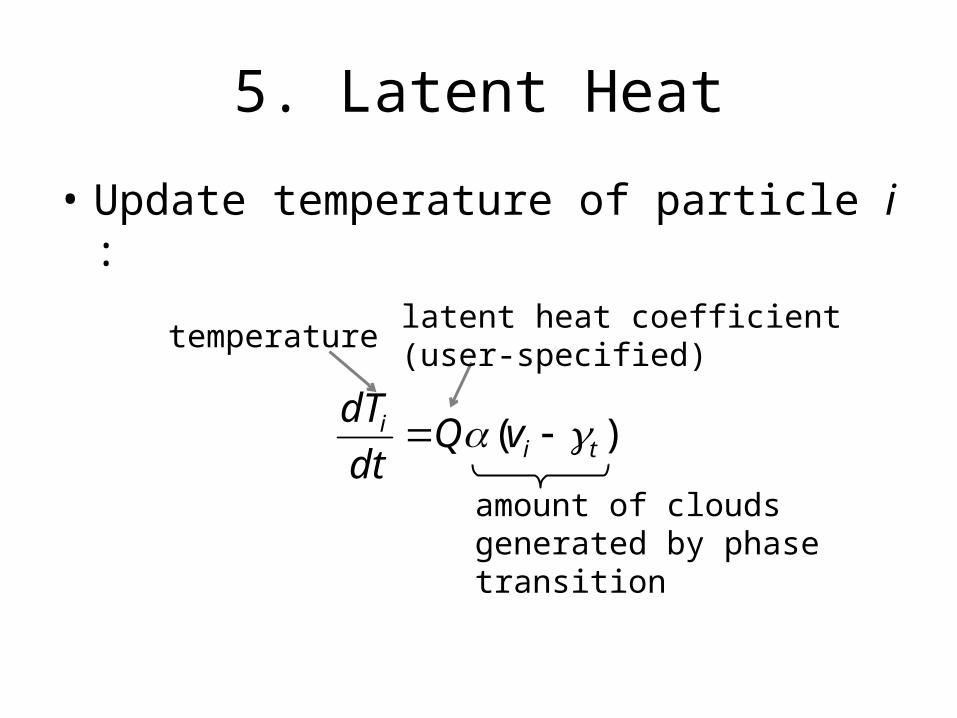
5. Latent Heat
• Update temperature of particle i :
)( tii vQdt
dT
temperaturelatent heat coefficient(user-specified)
amount of clouds generated by phase transition
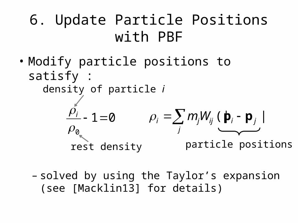
6. Update Particle Positions with PBF
• Modify particle positions to satisfy :
– solved by using the Taylor’s expansion(see [Macklin13] for details)
010
i
density of particle i
rest density
|)(| jij
ijji Wm pp
particle positions
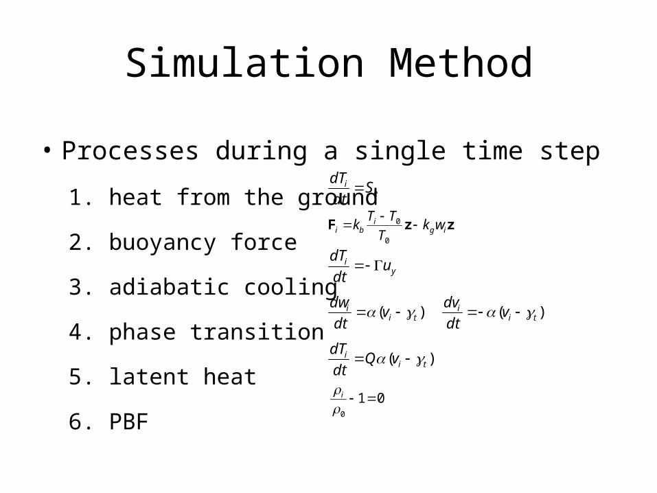
Simulation Method
• Processes during a single time step
1. heat from the ground
2. buoyancy force
3. adiabatic cooling
4. phase transition
5. latent heat
6. PBF
ei Sdt
dT
zzF igi
bi wkT
TTk
0
0
yi udt
dT
)( tii v
dt
dw )( tii vdt
dv
)( tii vQdt
dT
010
i

Experimental Result (2D)
• Scattered and unrealistic clouds• Smoothing of temperature field
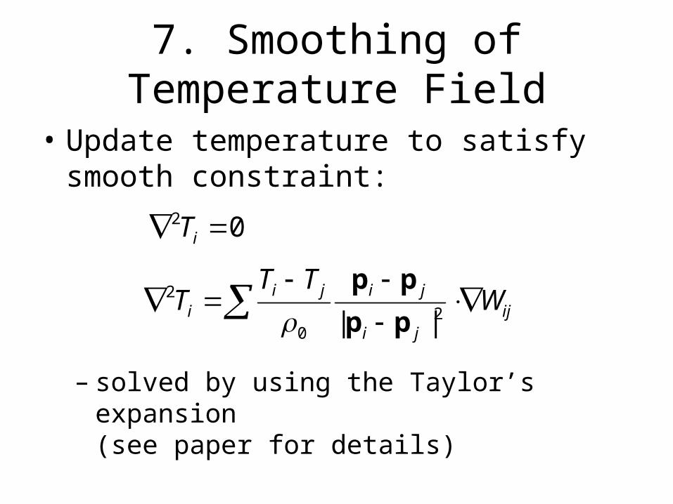
7. Smoothing of Temperature Field
• Update temperature to satisfy smooth constraint:
– solved by using the Taylor’s expansion(see paper for details)
02 iT
ijji
jijii W
TTT
20
2
|| pp
pp
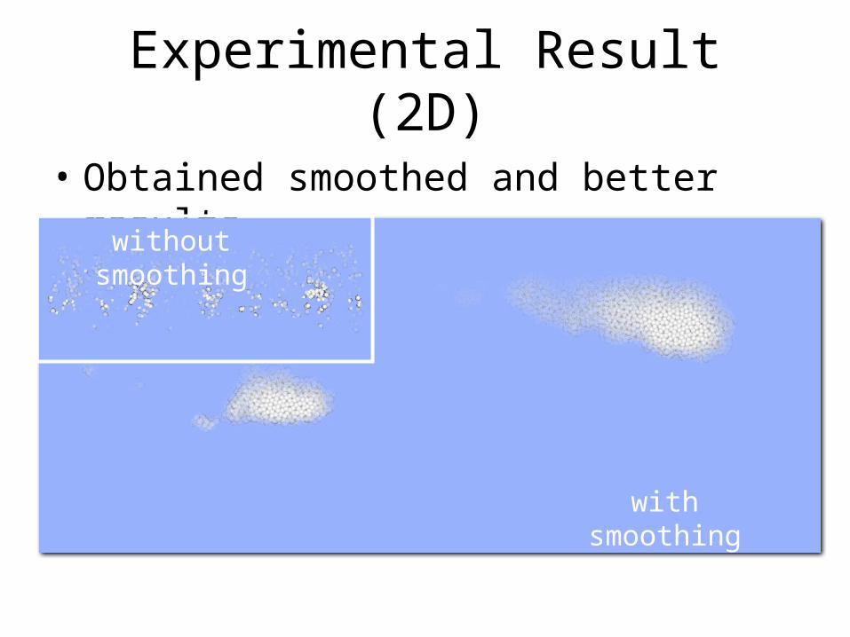
Experimental Result (2D)
• Obtained smoothed and better results
without smoothing
with smoothing
Proposed Method
• Overview of Cloud Formation Process• Simulation method• Adaptive particles
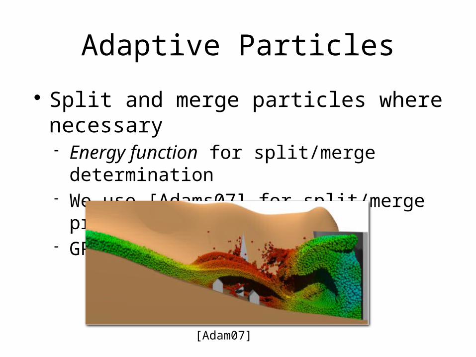
Adaptive Particles
Split and merge particles where necessary Energy function for split/merge determination We use [Adams07] for split/merge processes GPU implementation
[Adam07]

Energy Function
• Areas of interest : cloud regions– split where clouds are generated– merge where clouds disappear
• Simple energy function using cloud density:
)exp(1 icwkE cloud density
user-specified coefficient

Energy Function
)exp(1 icwkE
wi (cloud density)
E (s
hape
ene
rgy)
user-specified thresholds
cloud forming, split
no clouds, merge

GPU Implementation
• Split : straight forward• Merge : incorrect merging

GPU Implementation
• Split : straight forward• Merge : incorrect merging

GPU Implementation
• Split : straight forward• Merge : incorrect merging
thread 2
thread 3
thread 1

GPU Implementation
• Split : straight forward• Merge : incorrect merging
thread 2
thread 3
thread 1 thread 1

GPU Implementation
• Split : straight forward• Merge : incorrect merging
thread 2
thread 3
thread 1 thread 1 thread 2

GPU Implementation
• Split : straight forward• Merge : incorrect merging
thread 2
thread 3
thread 1 thread 1 thread 2
thread 3

GPU Implementation
• Split : straight forward• Merge : incorrect merging
thread 2
thread 3
thread 1
independentmerging
thread 2
thread 3
thread 1

GPU Implementation
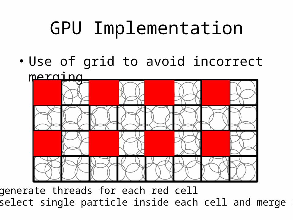
• Use of grid to avoid incorrect merging

GPU Implementation
• Use of grid to avoid incorrect merging

GPU Implementation
• Use of grid to avoid incorrect merging
generate threads for each red cell
GPU Implementation
• Use of grid to avoid incorrect merging
generate threads for each red cellselect single particle inside each cell and merge it

GPU Implementation
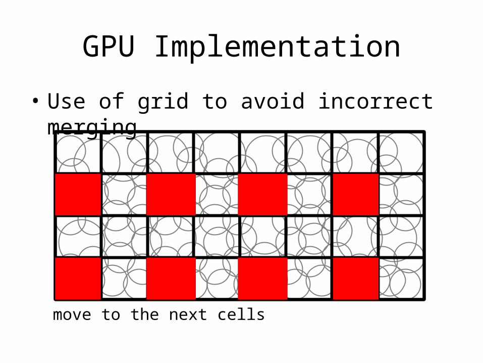
• Use of grid to avoid incorrect merging
move to the next cells

GPU Implementation
• Use of grid to avoid incorrect merging
select single particle inside each cell and merge it
GPU Implementation
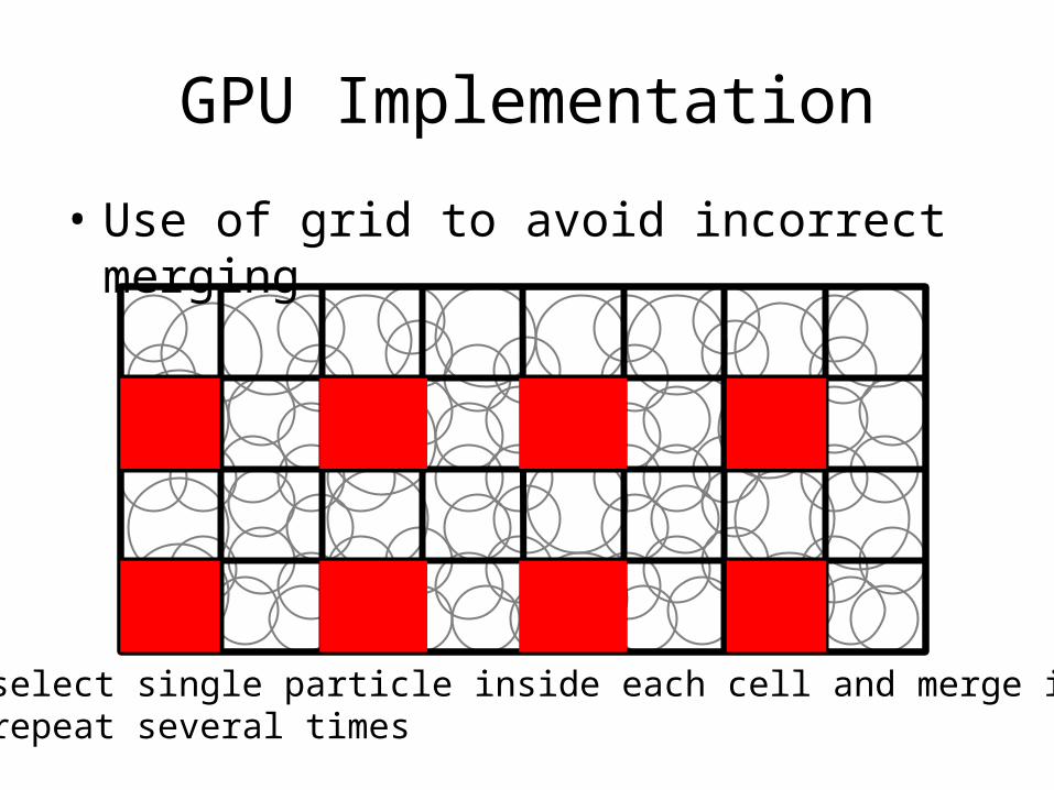
• Use of grid to avoid incorrect merging
move to the next cells
GPU Implementation
• Use of grid to avoid incorrect merging
select single particle inside each cell and merge it repeat several times
GPU Implementation
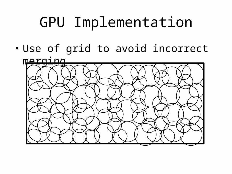
• Use of grid to avoid incorrect merging

Experimental Result (2D)
cloud density

Experimental Result (2D)
energy function

Experimental Result (2D)
subdivision level
Overview
• Introduction• Related Work• Proposed Method• Results• Conclusion
Results
• Computer– CPU: Corei7-4770K, 16 GB memory– GPU: NVIDIA GeForce GTX 780 Ti
• Rendering – mental ray (Autodesk MAYA 2014)
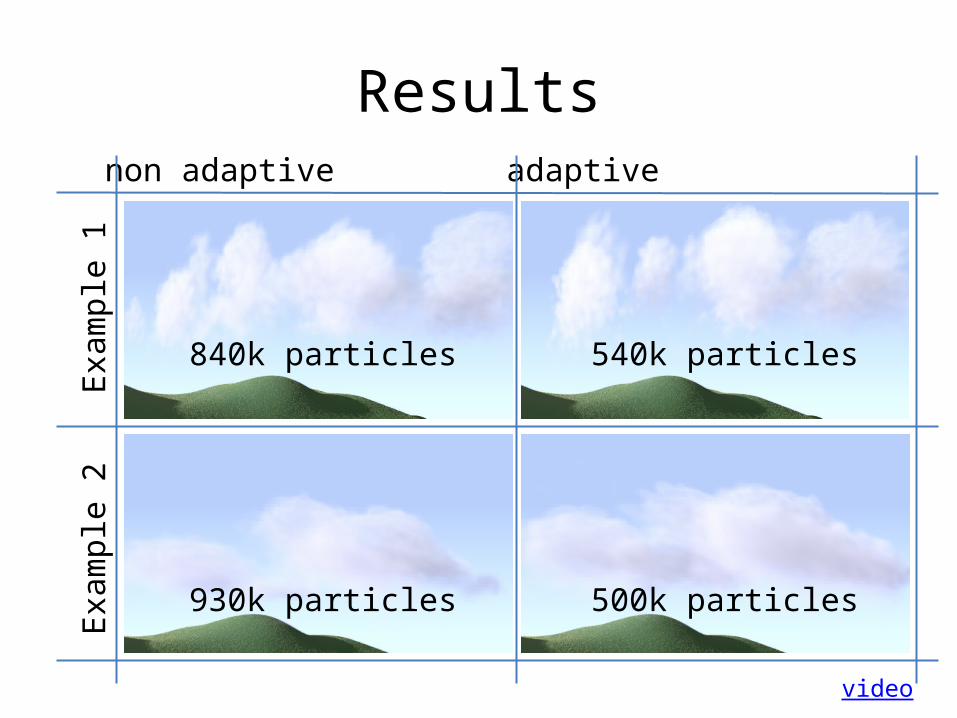
ResultsEx
ampl
e 1
Exam
ple
2
non adaptive adaptive
840k particles 540k particles
930k particles 500k particles
video

Results
• Average performance for single time stepPBF Smoothing Cloud
DynamicsSplit/Merge
Total
Ex. 1 (w/o adaptive) 1087 112 19 - 1218
Ex. 1(w adaptive) 629 65 13 30 737
Ex. 2(w/o adaptive) 1292 137 20 - 1449
Ex. 2(w adaptive) 749 72 14 31 866
[milliseconds]

Results
• Average performance for single time stepPBF Smoothing Cloud
DynamicsSplit/Merge
Total
Ex. 1 (w/o adaptive) 1087 112 19 - 1218
Ex. 1(w adaptive) 629 65 13 30 737
Ex. 2(w/o adaptive) 1292 137 20 - 1449
Ex. 2(w adaptive) 749 72 14 31 866
[milliseconds]
1.6x faster when using adaptive method
Conclusions/Future Work
• Particle-based cloud simulation– position-based fluids– smoothing of temperature field– adaptive method– GPU implementation
• Future Work– detailed shapes and motions