adabag: an r package for classification with boosting … · among the family of boosting...

JSS Journal of Statistical SoftwareAugust 2013, Volume 54, Issue 2. http://www.jstatsoft.org/

adabag: An R Package for Classification with

Boosting and Bagging

Esteban AlfaroUniversity of

Castilla-La Mancha

Matıas GamezUniversity of

Castilla-La Mancha

Noelia GarcıaUniversity of

Castilla-La Mancha

Abstract

Boosting and bagging are two widely used ensemble methods for classification. Theircommon goal is to improve the accuracy of a classifier combining single classifiers which areslightly better than random guessing. Among the family of boosting algorithms, AdaBoost(adaptive boosting) is the best known, although it is suitable only for dichotomous tasks.AdaBoost.M1 and SAMME (stagewise additive modeling using a multi-class exponentialloss function) are two easy and natural extensions to the general case of two or moreclasses. In this paper, the adabag R package is introduced. This version implementsAdaBoost.M1, SAMME and bagging algorithms with classification trees as base classifiers.Once the ensembles have been trained, they can be used to predict the class of newsamples. The accuracy of these classifiers can be estimated in a separated data set orthrough cross validation. Moreover, the evolution of the error as the ensemble growscan be analysed and the ensemble can be pruned. In addition, the margin in the classprediction and the probability of each class for the observations can be calculated. Finally,several classic examples in classification literature are shown to illustrate the use of thispackage.

Keywords: AdaBoost.M1, SAMME, bagging, R program, classification, classification trees.

1. Introduction

During the last decades, several new ensemble classification methods based in the tree struc-ture have been developed. In this paper, the package adabag for R (R Core Team 2013) isdecribed, which implements two of the most popular methods for ensembles of trees: boostingand bagging. The main difference between these two ensemble methods is that while boostingconstructs its base classifiers in sequence, updating a distribution over the training examplesto create each base classifier, bagging (Breiman 1996) combines the individual classifiers built

http://www.jstatsoft.org/

2 adabag: Classification with Boosting and Bagging in R

in bootstrap replicates of the training set. Boosting is a family of algorithms and two ofthem are implemented here: AdaBoost.M1 (Freund and Schapire 1996) and SAMME (Zhu,Zou, Rosset, and Hastie 2009). To the best of our knowledge, the SAMME algorithm is notavailable in any other R package.

The package adabag 3.2, available from de Comprehesive R Archive Network at http://CRAN.R-project.org/package=adabag, is the current update of adabag that changes the measureof relative importance of the predictor variables using the gain of the Gini index given by avariable in a tree and, in the case of the boosting function, the weight of this tree. For thisgoal, the varImp function of the caret package (Kuhn 2008, 2012) is used to get the gain ofthe Gini index of the variables in each tree.

Previously, the version 3.0 introduced four important new features: AdaBoost-SAMME isimplemented; a new function errorevol shows the error of the ensembles according to thenumber of iterations; the ensembles can be pruned using the option newmfinal in the corre-sponding predict function; and the posterior probability of each class for every observationcan be obtained. In addition, the version 2.0 incorporated the function margins to calculatethe margins for the classifiers.

Since the first version of this package, in 2006, it has been used in several classification tasksfrom very different scientific fields such as: economics and finance (Alfaro, Garcıa, Gamez, andElizondo 2008; Chrzanowska, Alfaro, and Witkowska 2009; De Bock and Van den Poel 2011),automated content analysis (Stewart and Zhukov 2009), interpreting signals out-of-control inquality control (Alfaro, Alfaro, Gamez, and Garcıa 2009), advances in machine learning (DeBock, Coussement, and Van den Poel 2010; Krempl and Hofer 2008). Moreover, adabag isused in the R package digeR (Fan, Murphy, and Watson 2012) and at least in two R manuals(Maindonald and Braun 2010; Torgo 2010).

Apart from adabag, nowadays there are several R packages dealing with boosting methods.Among them, the most widely used are ada (Culp, Johnson, and Michailidis 2012), gbm(Ridgeway 2013) and mboost (Buhlmann and Hothorn 2007; Hothorn et al. 2013). They arereally useful and well-documented packages. However, it seems that they are more focusedon boosting for regression and dichotomous classification. For a more detailed revision ofboosting packages see the intriguing CRAN Task View: “Machine Learning & StatisticalLearning” maintained by Hothorn (2013).

The paper is organized as follows. In Section 2 a brief description of the ensemble algorithmsAdaBoost.M1, SAMME and bagging is given. Section 3 explains the package functions. Thereare eight functions, three of them are specific for each ensemble family and two of them arecommon for all methods. In addition, all the functions are illustrated through a well-knownclassification problem, the iris example. This data set, although very useful for academicpurposes, is too simple. Thus, Section 4 is dedicated to provide a deep insight into the workingof the package through two more complex classification data sets. Finally, some concludingremarks are drawn in Section 5.

2. Algorithms

In this section a brief description of boosting and bagging algorithms is given. Their commongoal is to improve the accuracy of the ensemble, combining single classifiers which are asprecise and different as possible. In both cases, heterogeneity is introduced by modifying the

http://CRAN.R-project.org/package=adabag

http://CRAN.R-project.org/package=adabag

Journal of Statistical Software 3

training set where the individual classifiers are built. However, the base classifier of eachboosting iteration depends on all the previous ones through the weight updating process,whereas in bagging they are independent. In addition, the final boosting ensemble usesweighted majority vote while bagging uses a simple majority vote.

2.1. Boosting

Boosting is a method that makes maximum use of a classifier by improving its accuracy. Theclassifier method is used as a subroutine to build an extremely accurate classifier in the trainingset. Boosting applies the classification system repeatedly on the training data, but in eachstep the learning attention is focused on different examples of this set using adaptive weights,wb(i). Once the process has finished, the single classifiers obtained are combined into a final,highly accurate classifier in the training set. The final classifier therefore usually achieves ahigh degree of accuracy in the test set, as various authors have shown both theoretically andempirically (Banfield, Hall, Bowyer, and Kegelmeyer 2007; Bauer and Kohavi 1999; Dietterich2000; Freund and Schapire 1997).

Even though there are several versions of the boosting algorithms (Schapire and Freund 2012;Friedman, Hastie, and Tibshirani 2000), the best known is AdaBoost (Freund and Schapire1996). However, it can be only applied to binary classification problems. Among the versionsof boosting algorithms for multiclass classification problems (Mukherjee and Schapire 2011),two of the most simple and natural extensions of AdaBoost have been chosen, which are calledAdaBoost.M1 and SAMME.

Firstly, the AdaBoost.M1 algorithm can be described as follows. Given a training set Tn ={(x1, y1), . . . , (xi, yi), . . . , (xn, yn)} where yi takes values in 1, 2, . . . , k. The weight wb(i) isassigned to each observation xi and is initially set to 1/n. This value will be updated aftereach step. A basic classifier, Cb(xi), is built on this new training set (Tb) and is applied toevery training example. The error of this classifier is represented by eb and is calculated as

eb =n∑

i=1

wb(i)I(Cb(xi) 6= yi) (1)

where I(·) is the indicator function which outputs 1 if the inner expression is true and 0otherwise.

From the error of the classifier in the b-th iteration, the constant αb is calculated and usedfor weight updating. Specifically, according to Freund and Schapire, αb = ln ((1− eb)/eb).However, Breiman (Breiman 1998) uses αb = 1/2 ln ((1− eb)/eb). Anyway, the new weightfor the (b+ 1)-th iteration will be

wb+1(i) = wb(i) exp (αbI(Cb(xi) 6= yi)) (2)

Later, the calculated weights are normalized to sum one. Consequently, the weights of thewrongly classified observations are increased, and the weights of the rightly classified aredecreased, forcing the classifier built in the next iteration to focus on the hardest examples.Moreover, differences in weight updating are greater when the error of the single classifieris low because if the classifier achieves a high accuracy then the few mistakes take on moreimportance. Therefore, the alpha constant can be interpreted as a learning rate calculatedas a function of the error made in each step. Moreover, this constant is also used in the finaldecision rule giving more importance to the individual classifiers that made a lower error.


1. Start with wb(i) = 1/n, i = 1, 2, . . . , n

2. Repeat for b = 1, 2, . . . , Ba) Fit the classifier Cb(xi) = {1, 2, . . . , k} using weights wb(i) on Tb

b) Compute: eb =∑n

i=1wb(i)I(Cb(xi) 6= yi) and αb = 1/2 ln ((1− eb)/eb)c) Update the weights wb+1(i) = wb(i) exp (αbI(Cb(xi) 6= yi)) and normalize them

3. Output the final classifier Cf (xi) = arg maxj∈Y∑B

b=1 αbI(Cb(xi) = j)

Table 1: AdaBoost.M1 algorithm.

1. Start with wb(i) = 1/n, i = 1, 2, . . . , n

2. Repeat for b = 1, 2, . . . , Ba) Fit the classifier Cb(xi) = {1, 2, . . . , k} using weights wb(i) on Tb

b) Compute: eb =∑n

i=1wb(i)I(Cb(xi) 6= yi) and αb = ln ((1− eb)/eb) + ln(k − 1)c) Update the weights wb+1(i) = wb(i) exp (αbI(Cb(xi) 6= yi)) and normalize them

3. Output the final classifier Cf (xi) = arg maxj∈Y∑B

b=1 αbI(Cb(xi) = j)

Table 2: SAMME algorithm.

This process is repeated every step for b = 1, . . . , B. Finally, the ensemble classifier calculates,for each class, the weighted sum of its votes. Therefore, the class with the highest vote isassigned. Specifically,

Cf (xi) = arg maxj∈Y

B∑b=1

αbI(Cb(xi) = j) (3)

Table 1 shows the complete AdaBoost.M1 pseudocode.

SAMME, the second boosting algorithm implemented here, is summarized in Table 2. Itis worth mentioning that the only difference between this algorithm and AdaBoost.M1 isthe way in which the alpha constant is calculated, because the number of classes is takeninto account in this case. Due to this modification, the SAMME algorithm only needs that1 − eb > 1/k in order for the alpha constant to be positive and the weight updating followsthe right direction. That is to say, the accuracy of each weak classifier should be better thanthe random guess (1/k) instead of 1/2, which would be an appropriate requirement for thetwo class case but very demanding for the multi-class one.

2.2. Bagging

Bagging is a method that combines bootstrapping and aggregating (Table 3). If the bootstrapestimate of the data distribution parameters is more accurate and robust than the traditionalone, then a similar method can be used to achieve, after combining them, a classifier with


1. Repeat for b = 1, 2, . . . , Ba) Take a bootstrap replicate Tb of the training set Tn

b) Construct a single classifier Cb(xi) = {1, 2, . . . , k} in Tb

2. Combine the basic classifiers Cb(xi), b = 1, 2, . . . , B by the majority vote (the most oftenpredicted class) to the final decission rule Cf (xi) = arg maxj∈Y

∑Bb=1 I(Cb(xi) = j)

Table 3: Bagging algorithm.

better properties.

On the basis of the training set (Tn), B bootstrap samples (Tb) are obtained, where b =1, 2, . . . , B. These bootstrap samples are obtained by drawing with replacement the samenumber of elements than the original set (n in this case). In some of these boostrap samples,the presence of noisy observations may be eliminated or at least reduced, (as there is a lowerproportion of noisy than non-noisy examples) so the classifiers built in these sets will have abetter behavior than the classifier built in the original set. Therefore, bagging can be reallyuseful to build a better classifier when there are noisy observations in the training set.

The ensemble usually achieves better results than the single classifiers used to build the finalclassifier. This can be understood since combining the basic classifiers also combines theadvantages of each one in the final ensemble.

2.3. The margin

In the boosting literature, the concept of margin (Schapire, Freund, Bartlett, and Lee 1998) isimportant. The margin for an object is intuitively related to the certainty of its classificationand is calculated as the difference between the support of the correct class and the maximumsupport of an incorrect class. For k classes, the margin of an example xi is calculated usingthe votes for every class j in the final ensemble, which are known as the degree of support ofthe different classes or posterior probabilities µj(xi), j = 1, 2, . . . , k as

m(xi) = µc(xi)−maxj 6=c

µj(xi) (4)

where c is the correct class of xi and∑k

j=1 µj(xi) = 1. All the wrongly classified examples willtherefore have negative margins and those correctly classified ones will have positive margins.Correctly classified observations with a high degree of confidence will have margins close toone. On the other hand, examples with an uncertain classification will have small margins,that is to say, margins close to zero. Since a small margin is an instability symptom in theassigned class, the same example could be assigned to different classes by similar classifiers.For visualization purposes, Kuncheva (2004) uses margin distribution graphs showing thecumulative distribution of the margins for a given data set. The x-axis is the margin (m) andthe y-axis is the number of points where the margin is less than or equal to m. Ideally, allpoints should be classified correctly so that all the margins are positive. If all the points havebeen classified correctly and with the maximum possible certainty, the cumulative graph willbe a single vertical line at m = 1.


3. Functions

In this section, the functions of the adabag package in R are explained. As mentioned before,it implements AdaBoost.M1, SAMME and bagging with classification and regression trees,(CART, Breiman, Friedman, Olshenn, and Stone 1984) as base classifiers using the rpartpackage (Therneau, Atkinson, and Ripley 2013). Here boosted or bagged trees are used,although these algorithms can be used with other basic classifiers. Therefore, ahead in thepaper boosting or bagging refer to boosted trees or bagged trees.

This package consists of a total of eight functions, three for each method and the margins andevolerror. The three functions for each method are: one to build the boosting (or bagging)classifier and classify the samples in the training set; one which can predict the class of newsamples using the previously trained ensemble; and lastly, another which can estimate bycross validation the accuracy of these classifiers in a data set. Finally, the margin in the classprediction for each observation and the error evolution can be calculated.

3.1. The boosting, predict.boosting and boosting.cv functions

As aforementioned, there are three functions with regard to the boosting method in theadabag package. Firstly, the boosting function enables to build an ensemble classifier usingAdaBoost.M1 or SAMME and assign a class to the training samples. Any function in Rrequires a set of initial arguments to be fixed; in this case, there are six of them. Theformula, as in the lm function, spells out the dependent and independent variables. Thedata frame in which to interpret the variables named in formula. It collects the data to beused for training the ensemble. If the logical parameter boos is TRUE (by default), a bootstrapsample of the training set is drawn using the weight for each observation on that iteration. Ifboos is FALSE, every observation is used with its weight. The integer mfinal sets the numberof iterations for which boosting is run or the number of trees to use (by default mfinal =

100 iterations).

If the logical argument coeflearn = "Breiman" (by default), then alpha = 1/2 ln((1−eb)/eb)is used. However, if coeflearn = "Freund", then alpha = ln((1 − eb)/eb) is used. In bothcases the AdaBoost.M1 algorithm is applied and alpha is the weight updating coefficient.On the other hand, if coeflearn = "Zhu", the SAMME algorithm is used with alpha =ln((1− eb)/eb) + ln(k − 1). As above mentioned, the error of the single trees must be in therange (0, 0.5) for AdaBoost.M1, while for SAMME in the range (0, 1−1/k). In the case wherethese assumptions are not fulfilled, Opitz and Maclin (Opitz and Maclin 1999) reset all theweigths to be equal, choose appropriate values to weight these trees and restart the process.The same solution is applied here. When eb = 0, the alpha constant is calculated usingeb = 0.001 and when eb ≥ 0.5 (eb ≥ 1−1/k for SAMME), it is replaced by 0.499 (0.999−1/k,respectively).

Lastly, the option control that regulates details of the rpart function is also transferred toboosting specially to limit the size of the trees in the ensemble. See rpart.control for moredetails.

Upon applying boosting and training the ensemble, this function outputs an object of classboosting, which is a list with seven components. The first one is the formula used to trainthe ensemble. Secondly, the trees which have been grown along the iterations are shown.A vector which depicts the weights of the trees. The votes matrix describing, for each


observation, the number of trees that assigned it to each class, weighting each tree by itsalpha coefficient. The prob matrix showing, for each observation, an approximation to theposterior probability achieved in each class. This estimation of the probabilities is calculatedusing the proportion of votes or support in the final ensemble. The class vector is theclass predicted by the ensemble classifier. Finally, the importance vector returns the relativeimportance or contribution of each variable in the classification task.

It is worth to highlight that the boosting function allows quantifying the relative importanceof the predictor variables. Understanding a small individual tree can be easy. However,it is more difficult to interpret the hundreds or thousands of trees used in the boostingensemble. Therefore, to be able to quantify the contribution of the predictor variables tothe discrimination is a really important advantage. The measure of importance takes intoaccount the gain of the Gini index given by a variable in a tree and the weight of this tree inthe case of boosting. For this goal, the varImp function of the caret package is used to getthe gain of the Gini index of the variables in each tree.

The well-known iris data set is used as an example to illustrate the use of adabag. Thepackage is loaded using library("adabag") and automatically the program calls the requiredpackages rpart, caret and mlbench (Leisch and Dimitriadou 2012).

The dataset is randomly divided into two equal size sets. The training set is classified with aboosting ensemble of 10 trees of maximum depth 1 (stumps) using the code below. The listreturned consists of the formula used, the 10 small trees and the weights of the trees. Thelower the error of a tree, the higher its weight. In other words, the lower the error of a tree,the more relevant in the final ensemble. In this case, there is a tie among four trees with thehighest weights (numbers 3, 4, 5 and 6). On the other hand, tree number 9 has the lowestweight (0.175). The matrices votes and prob show the weighted votes and probabilities thateach observation (rows) receives for each class (columns). For instance, the first observationreceives 2.02 votes for the first, 0.924 for the second and 0 for the third class. Therefore, theprobabilities for each class are 68.62%, 31.38% and 0%, respectively, and the assigned class is"setosa" as can be seen in the class vector.

R> library("adabag")

R> data("iris")

R> train <- c(sample(1:50, 25), sample(51:100, 25), sample(101:150, 25))

R> iris.adaboost <- boosting(Species ~ ., data = iris[train, ], mfinal = 10,

+ control = rpart.control(maxdepth = 1))

R> iris.adaboost

$formula

Species ~ .

$trees

$trees[[1]]

n = 75

node), split, n, loss, yval, (yprob)

* denotes terminal node


1) root 75 46 virginica (0.29333333 0.32000000 0.38666667)

2) Petal.Length < 4.8 44 22 setosa (0.50000000 0.50000000 0.00000000) *

3) Petal.Length >= 4.8 31 2 virginica (0.00000000 0.06451613 0.93548387) *

$trees[[2]]

n= 75



1) root 75 40 versicolor (0.22666667 0.46666667 0.30666667)

2) Petal.Width < 1.7 53 18 versicolor (0.32075472 0.66037736 0.01886792) *

3) Petal.Width >= 1.7 22 0 virginica (0.00000000 0.00000000 1.00000000) *

...

$trees[[10]]

n= 75



1) root 75 42 virginica (0.21333333 0.34666667 0.44000000)

2) Petal.Width < 1.7 46 20 versicolor (0.34782609 0.56521739 0.08695652) *

3) Petal.Width >= 1.7 29 0 virginica (0.00000000 0.00000000 1.00000000) *

$weights

[1] 0.3168619 0.2589715 0.3465736 0.3465736 0.3465736 0.3465736 0.2306728

[8] 0.3168619 0.1751012 0.2589715

$votes

[,1] [,2] [,3]

[1,] 2.0200181 0.923717 0.0000000

[2,] 2.0200181 0.923717 0.0000000

...

[25,] 2.0200181 0.923717 0.0000000

[26,] 0.6337238 1.963438 0.3465736

[27,] 0.0000000 1.732765 1.2109701

...

[50,] 0.6337238 1.788337 0.5216748

[51,] 0.0000000 1.039721 1.9040144

[52,] 0.0000000 1.039721 1.9040144

...

[74,] 0.0000000 1.039721 1.9040144

[75,] 0.0000000 1.039721 1.9040144

$prob


[,1] [,2] [,3]

[1,] 0.6862092 0.3137908 0.0000000

[2,] 0.6862092 0.3137908 0.0000000

...

[25,] 0.6862092 0.3137908 0.0000000

[26,] 0.2152788 0.6669886 0.1177326

[27,] 0.0000000 0.588628 0.411372

...

[50,] 0.2152788 0.6075060 0.1772152

[51,] 0.0000000 0.3531978 0.6468022

[52,] 0.0000000 0.3531978 0.6468022

...

[74,] 0.0000000 0.3531978 0.6468022

[75,] 0.0000000 0.3531978 0.6468022

$class

[1] "setosa" "setosa" "setosa" "setosa" "setosa"





[26] "versicolor" "versicolor" "versicolor" "versicolor" "versicolor"





[51] "virginica" "virginica" "virginica" "virginica" "virginica"

[56] "virginica" "virginica" "virginica" "versicolor" "virginica"


[66] "virginica" "virginica" "virginica" "versicolor" "versicolor"

[71] "virginica" "virginica" "versicolor" "virginica" "virginica"

$importance

Sepal.Length Sepal.Width Petal.Length Petal.Width

0 0 83.20452 16.79548

attr(,"class")

[1] "boosting"

From the importance vector it can be drawn that Petal.Length is the most importantvariable, as it achieved 83.20% of the information gain. It can be graphically seen in Figure 1.

R> barplot(iris.adaboost$imp[order(iris.adaboost$imp, decreasing = TRUE)],

+ ylim = c(0, 100), main = "Variables Relative Importance",

+ col = "lightblue")

From the iris.adaboost object it is easy to build the confusion matrix for the training set


Petal.Length Petal.Width Sepal.Length Sepal.Width

Variables relative importance

020

4060

8010

0

Figure 1: Variables relative importance for boosting in the iris example.

and calculate the error. In this case, four flowers from class virginica were classified asversicolor, so the achieved error was 5.33%.

R> table(iris.adaboost$class, iris$Species[train],

+ dnn = c("Predicted Class", "Observed Class"))

Observed Class

Predicted Class setosa versicolor virginica

setosa 25 0 0

versicolor 0 25 4

virginica 0 0 21

R> 1 - sum(iris.adaboost$class == iris$Species[train]) /

+ length(iris$Species[train])

[1] 0.05333333

The second function predict.boosting matches the parameters of the generic functionpredict and adds one more (object,newdata,newmfinal = length(objects$trees),...).It classifies a data frame using a fitted model object of class boosting. This is assumed tobe the result of some function that produces an object with the same named components asthose returned by the boosting function. The newdata argument is a data frame containingthe values for which predictions are required. The predictors referred to in the right sideof formula(object) must be present here with the same name. This way, predictions be-yond the training data can be made. The newmfinal option fixes the number of trees of theboosting object to be used in the prediction. This allows the user to prune the ensemble. Bydefault, all the trees in the object are used. Lastly, the three dots deal with further argumentspassed to or from other methods.


On the other hand, this function returns an object of class predict.boosting, which is a listwith the following six components. Four of them: formula, votes, prob and class have thesame meaning as in the boosting output. In addition, the confusion matrix compares thereal class with the predicted one and, lastly, the average error is computed.

Following with the example, the iris.adaboost classifier can be used to predict the class fornew iris examples by means of the predict.boosting function, as it is shown below andthe ensemble can also be pruned. The first four components of the output are common tothe previous function output but the confusion matrix and the test data set error are hereadditionally provided. In this case, three virginica iris from the test data set were classifiedas versicolor class, so the error in this case reached 4%.

R> iris.predboosting <- predict.boosting(iris.adaboost,

+ newdata = iris[-train, ])

R> iris.predboosting

$formula

Species ~ .

$votes

[,1] [,2] [,3]

[1,] 2.0200181 0.923717 0.0000000

[2,] 2.0200181 0.923717 0.0000000

...

[25,] 2.0200181 0.923717 0.0000000

[26,] 0.6337238 1.963438 0.3465736

[27,] 0.6337238 1.963438 0.3465736

...

[50,] 0.6337238 1.963438 0.3465736

[51,] 0.0000000 1.039721 1.9040144

[52,] 0.0000000 1.039721 1.9040144

...

[74,] 0.0000000 1.039721 1.9040144

[75,] 0.0000000 1.039721 1.9040144

$prob

[,1] [,2] [,3]

[1,] 0.6862092 0.3137908 0.0000000

[2,] 0.6862092 0.3137908 0.0000000

...

[25,] 0.6862092 0.3137908 0.0000000

[26,] 0.2152788 0.6669886 0.1177326

[27,] 0.2152788 0.6669886 0.1177326

...

[50,] 0.2152788 0.6669886 0.1177326

[51,] 0.0000000 0.3531978 0.6468022

[52,] 0.0000000 0.3531978 0.6468022

...


[74,] 0.0000000 0.3531978 0.6468022

[75,] 0.0000000 0.3531978 0.6468022

$class











[51] "virginica" "virginica" "virginica" "virginica" "versicolor"


[61] "virginica" "virginica" "virginica" "virginica" "versicolor"



$confusion

Observed Class


setosa 25 0 0

versicolor 0 25 3

virginica 0 0 22

$error

[1] 0.04

Finally, the third function boosting.cv runs v-fold cross validation with boosting. As usuallyin cross validation, the data are divided into v non-overlapping subsets of roughly equal size.Then, boosting is applied on (v − 1) of the subsets. Lastly, predictions are made for the leftout subset, and the process is repeated for each one of the v subsets.

The arguments of this function are the same seven of boosting and one more, an integer v,specifying the type of v-fold cross validation. The default value is 10. On the contrary, if v isset as the number of observations, leave-one-out cross validation is carried out. Besides this,every value between two and the number of observations is valid and means that one out ofevery v observations is left out. An object of class boosting.cv is supplied, which is a listwith three components, class, confusion and error, which have been previously describedin the predict.boosting function.

Therefore, cross validation can be used to estimate the error of the ensemble without dividingthe available data set into training and test subsets. This is specially advantageous for smalldata sets.

Returning to the iris example, 10-folds cross validation is applied maintaining the numberand size of the trees. The output components are: a vector with the assigned class, the


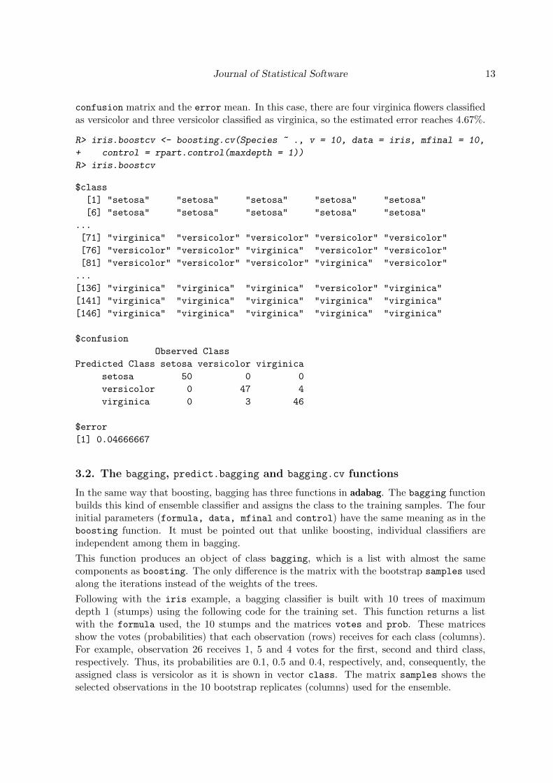
confusion matrix and the error mean. In this case, there are four virginica flowers classifiedas versicolor and three versicolor classified as virginica, so the estimated error reaches 4.67%.

R> iris.boostcv <- boosting.cv(Species ~ ., v = 10, data = iris, mfinal = 10,


R> iris.boostcv

$class



...

[71] "virginica" "versicolor" "versicolor" "versicolor" "versicolor"

[76] "versicolor" "versicolor" "virginica" "versicolor" "versicolor"

[81] "versicolor" "versicolor" "versicolor" "virginica" "versicolor"

...




$confusion

Observed Class


setosa 50 0 0

versicolor 0 47 4

virginica 0 3 46

$error

[1] 0.04666667

3.2. The bagging, predict.bagging and bagging.cv functions

In the same way that boosting, bagging has three functions in adabag. The bagging functionbuilds this kind of ensemble classifier and assigns the class to the training samples. The fourinitial parameters (formula, data, mfinal and control) have the same meaning as in theboosting function. It must be pointed out that unlike boosting, individual classifiers areindependent among them in bagging.

This function produces an object of class bagging, which is a list with almost the samecomponents as boosting. The only difference is the matrix with the bootstrap samples usedalong the iterations instead of the weights of the trees.

Following with the iris example, a bagging classifier is built with 10 trees of maximumdepth 1 (stumps) using the following code for the training set. This function returns a listwith the formula used, the 10 stumps and the matrices votes and prob. These matricesshow the votes (probabilities) that each observation (rows) receives for each class (columns).For example, observation 26 receives 1, 5 and 4 votes for the first, second and third class,respectively. Thus, its probabilities are 0.1, 0.5 and 0.4, respectively, and, consequently, theassigned class is versicolor as it is shown in vector class. The matrix samples shows theselected observations in the 10 bootstrap replicates (columns) used for the ensemble.


R> iris.bagging <- bagging(Species ~ ., data = iris[train, ], mfinal = 10,


R> iris.bagging

$formula

Species ~ .

$trees

$trees[[1]]

n= 75



1) root 75 47 setosa (0.3733333 0.3333333 0.2933333)

2) Petal.Length< 2.45 28 0 setosa (1.0000000 0.0000000 0.0000000) *

3) Petal.Length>=2.45 47 22 versicolor (0.0000000 0.5319149 0.4680851) *

$trees[[2]]

n= 75



1) root 75 46 setosa (0.3866667 0.2933333 0.3200000)


3) Petal.Length>=2.35 46 22 virginica (0.0000000 0.4782609 0.5217391) *

...

$trees[[10]]

n= 75



1) root 75 45 versicolor (0.3066667 0.4000000 0.2933333)


3) Petal.Length>=2.45 52 22 versicolor (0.0000000 0.5769231 0.4230769) *

$votes

[,1] [,2] [,3]

[1,] 9 1 0

[2,] 9 1 0

...

[25,] 9 1 0

[26,] 1 5 4

[27,] 1 5 4


...

[50,] 1 5 4

[51,] 0 4 6

[52,] 0 4 6

...

[74,] 0 4 6

[75,] 0 4 6

$prob

[,1] [,2] [,3]

[1,] 0.9 0.1 0

[2,] 0.9 0.1 0

...

[25,] 0.9 0.1 0

[26,] 0.1 0.5 0.4

[27,] 0.1 0.5 0.4

...

[50,] 0.1 0.5 0.4

[51,] 0 0.4 0.6

[52,] 0 0.4 0.6

...

[74,] 0 0.4 0.6

[75,] 0 0.4 0.6

$class












[56] "versicolor" "virginica" "versicolor" "virginica" "virginica"




$samples

[,1] [,2] [,3] [,4] [,5] [,6] [,7] [,8] [,9] [,10]

[1,] 8 21 53 16 75 71 15 47 73 7

[2,] 58 60 65 36 51 18 29 74 65 4

[3,] 74 21 22 24 72 14 34 27 22 26

[4,] 39 26 6 16 66 29 70 32 1 28


Petal.Length Petal.Width Sepal.Length Sepal.Width


020

4060

8010

0

Figure 2: Variables relative importance for bagging in the iris example.

[5,] 26 17 42 36 53 4 46 75 21 22

...

[71,] 3 28 13 55 53 23 64 17 27 36

[72,] 23 24 53 54 42 53 2 44 48 32

[73,] 16 17 69 12 50 15 34 30 7 42

[74,] 43 46 29 70 50 37 61 50 73 35

[75,] 45 44 13 75 19 67 49 68 1 67

$importance

Sepal.Length Sepal.Width Petal.Length Petal.Width

0 0 79.69223 20.30777

attr(,"class")

[1] "bagging"

In line with boosting, the variables with the highest contributions are Petal.Length (79.69%)and Petal.Width (20.31%). On the contrary, the contribution of the other two variables iszero. It is graphically shown in Figure 2.

R> barplot(iris.bagging$imp[order(iris.bagging$imp, decreasing = TRUE)],

+ ylim = c(0, 100), main = "Variables Relative Importance",

+ col = "lightblue")

The object iris.bagging can be used to compute the confusion matrix and the training seterror. As can be seen, only two cases are wrongly classified (two virginica flowers classifiedas versicolor), therefore the error is 2.67%.

R> table(iris.bagging$class, iris$Species[train],



Observed Class


setosa 25 0 0

versicolor 0 25 2

virginica 0 0 23

R> 1 - sum(iris.bagging$class == iris$Species[train]) /

+ length(iris$Species[train])

[1] 0.02666667

In addition, predict.bagging has the same arguments and values as predict.boosting.However, it calls a fitted bagging object and returns an object of class predict.bagging.Finally, bagging.cv runs v-fold cross validation with bagging. Again, the type of v-fold crossvalidation is added to the arguments of the bagging function. Moreover, the output is anobject of class bagging.cv similar to boosting.cv.

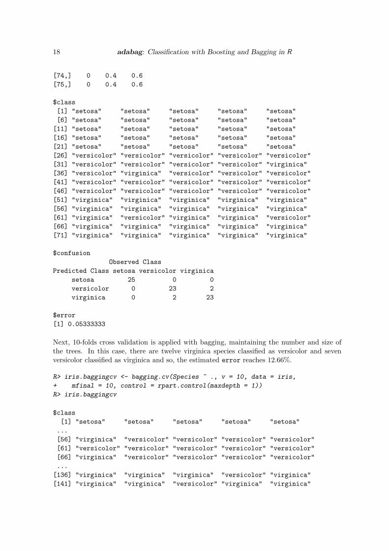
The function predict.bagging uses the previously built object iris.bagging to predict theclass for each observation in the test data set and to prune it, if necessary. The output isthe same as in predict.boosting. In this case, the confusion matrix shows two virginicaspecies classified as versicolor and vice versa, so the error is 5.33%.

R> iris.predbagging <- predict.bagging(iris.bagging, newdata = iris[-train, ])

R> iris.predbagging

$formula

Species ~ .

$votes

[,1] [,2] [,3]

[1,] 9 1 0

[2,] 9 1 0

...

[26,] 1 5 4

[27,] 1 5 4

...

[74,] 0 4 6

[75,] 0 4 6

$prob

[,1] [,2] [,3]

[1,] 0.9 0.1 0

[2,] 0.9 0.1 0

...

[26,] 0.1 0.5 0.4

[27,] 0.1 0.5 0.4

...


[74,] 0 0.4 0.6

[75,] 0 0.4 0.6

$class







[31] "versicolor" "versicolor" "versicolor" "versicolor" "virginica"

[36] "versicolor" "virginica" "versicolor" "versicolor" "versicolor"





[61] "virginica" "versicolor" "virginica" "virginica" "versicolor"



$confusion

Observed Class


setosa 25 0 0

versicolor 0 23 2

virginica 0 2 23

$error

[1] 0.05333333

Next, 10-folds cross validation is applied with bagging, maintaining the number and size ofthe trees. In this case, there are twelve virginica species classified as versicolor and sevenversicolor classified as virginica and so, the estimated error reaches 12.66%.

R> iris.baggingcv <- bagging.cv(Species ~ ., v = 10, data = iris,

+ mfinal = 10, control = rpart.control(maxdepth = 1))

R> iris.baggingcv

$class


...




...


[141] "virginica" "virginica" "versicolor" "virginica" "virginica"



$confusion

Clase real

Clase estimada setosa versicolor virginica

setosa 50 0 0

versicolor 0 43 12

virginica 0 7 38

$error

[1] 0.1266667

3.3. The margins and errorevol functions

Owing to its aforementioned importance the margins function was added to adabag to cal-culate the margins of a boosting or bagging classifier for a data frame as previously definedin Equation 4. Its usage is very easy with only two arguments:

1. object. This object must be the output of one of the functions bagging, boosting,predict.bagging or predict.boosting. This is assumed to be the result of somefunction that produces an object with at least two components named formula andclass, as those returned for instance by the bagging function.

2. newdata. The same data frame used for building the object.

The output, an object of class margins, is a simple list with only one vector with the margins.In the following it is shown the code to calculate the margins of the bagging classifier builtin the previous section, for the training and test sets, respectively. Examples with negativemargins are those which have been wrongly classified. As it was stated before, there were twoand four cases in each set, respectively.

R> iris.bagging.margins <- margins(iris.bagging, iris[train, ])

R> iris.bagging.predmargins <- margins(iris.predbagging, iris[-train, ])

R> iris.bagging.margins

$margins

[1] 0.8 0.8 0.8 0.8 0.8 0.8 0.8 0.8 0.8 0.8 0.8 0.8 0.8 0.8

[15] 0.8 0.8 0.8 0.8 0.8 0.8 0.8 0.8 0.8 0.8 0.8 0.1 0.1 0.1

[29] 0.1 0.1 0.1 0.1 0.1 0.1 0.1 0.1 0.1 0.1 0.1 0.1 0.1 0.1

[43] 0.1 0.1 0.1 0.1 0.1 0.1 0.1 0.1 0.2 0.2 0.2 0.2 0.2 -0.1

[57] 0.2 -0.1 0.2 0.2 0.2 0.2 0.2 0.2 0.2 0.2 0.2 0.2 0.2 0.2

[71] 0.2 0.2 0.2 0.2 0.2

R> iris.bagging.predmargins

$margins

[1] 0.8 0.8 0.8 0.8 0.8 0.8 0.8 0.8 0.8 0.8 0.8 0.8 0.8 0.8


−1.0 −0.5 0.0 0.5 1.0

0.0

0.2

0.4

0.6

0.8

1.0

Margin cumulative distribution graph

m

% o

bser

vatio

ns

test

train

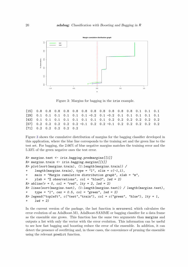
Figure 3: Margins for bagging in the iris example.

[15] 0.8 0.8 0.8 0.8 0.8 0.8 0.8 0.8 0.8 0.8 0.8 0.1 0.1 0.1

[29] 0.1 0.1 0.1 0.1 0.1 0.1 -0.2 0.1 -0.2 0.1 0.1 0.1 0.1 0.1

[43] 0.1 0.1 0.1 0.1 0.1 0.1 0.1 0.1 0.2 0.2 0.2 0.2 0.2 0.2

[57] 0.2 0.2 0.2 0.2 0.2 -0.1 0.2 0.2 -0.1 0.2 0.2 0.2 0.2 0.2

[71] 0.2 0.2 0.2 0.2 0.2

Figure 3 shows the cumulative distribution of margins for the bagging classifier developed inthis application, where the blue line corresponds to the training set and the green line to thetest set. For bagging, the 2.66% of blue negative margins matches the training error and the5.33% of the green negative ones the test error.

R> margins.test <- iris.bagging.predmargins[[1]]

R> margins.train <- iris.bagging.margins[[1]]

R> plot(sort(margins.train), (1:length(margins.train)) /

+ length(margins.train), type = "l", xlim = c(-1,1),

+ main = "Margin cumulative distribution graph", xlab = "m",

+ ylab = "% observations", col = "blue3", lwd = 2)

R> abline(v = 0, col = "red", lty = 2, lwd = 2)

R> lines(sort(margins.test), (1:length(margins.test)) / length(margins.test),

+ type = "l", cex = 0.5, col = "green", lwd = 2)

R> legend("topleft", c("test","train"), col = c("green", "blue"), lty = 1,

+ lwd = 2)

In the current version of the package, the last function is errorevol which calculates theerror evolution of an AdaBoost.M1, AdaBoost-SAMME or bagging classifier for a data frameas the ensemble size grows. This function has the same two arguments than margins andoutputs a list with only the vector with the error evolution. This information can be usefulto see how fast bagging and boosting reduce the error of the ensemble. In addition, it candetect the presence of overfitting and, in those cases, the convenience of pruning the ensembleusing the relevant predict function.


2 4 6 8 10

0.0

0.2

0.4

0.6

0.8

1.0

Boosting error versus number of trees

Iterations

Err

or

test

train

Figure 4: Error evolution for boosting in the iris example.

Although, due to the small size of the ensembles, this example is not the most appropriatecase to show the error evolution usefulness, it is used just for demonstrative purposes.

R> evol.test <- errorevol(iris.adaboost, iris[-train, ])

R> evol.train <- errorevol(iris.adaboost, iris[train, ])

R> plot(evol.test$error, type = "l", ylim = c(0, 1),

+ main = "Boosting error versus number of trees", xlab = "Iterations",

+ ylab = "Error", col = "red", lwd = 2)

R> lines(evol.train$error, cex = .5, col = "blue", lty = 2, lwd = 2)

R> legend("topleft", c("test", "train"), col = c("red", "blue"), lty = 1:2,

+ lwd = 2)

4. Examples

The package adabag is now more deeply illustrated through other two classification examples.The first example shows a dichotomous classification problem using a simulated dataset previ-ously used by Hastie, Tibshirani, and Friedman (2001, pp. 301–309) and Culp, Johnson, andMichailides (2006). The second example is a four classes data set from the UCI repository ofmachine learning databases (Bache and Lichman 2013). This example and iris are availablein the base and mlbench R packages.

4.1. A dichotomous example

The two classes simulated data set consists of ten standard independent Gaussians which areused as features and the two classes defined as

Y =

{1

∑X2

j > 9.34

−1 otherwise(5)

Here the value 9.34 is the median of a Chi-squared random variable with 10 degrees of freedom(sum of squares of 10 standard Gaussians). There are 2000 training and 10000 test cases,


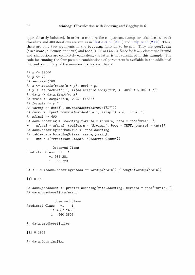
approximately balanced. In order to enhance the comparison, stumps are also used as weakclassifiers and 400 iterations are run as in Hastie et al. (2001) and Culp et al. (2006). Thus,there are only two arguments in the boosting function to be set. They are coeflearn

("Breiman", "Freund" or "Zhu") and boos (TRUE or FALSE). Since for k = 2 classes the Freundand Zhu options are completely equivalent, the latter is not considered in this example. Thecode for running the four possible combinations of parameters is available in the additionalfile, and a summary of the main results is shown below.

R> n <- 12000

R> p <- 10

R> set.seed(100)

R> x <- matrix(rnorm(n * p), ncol = p)

R> y <- as.factor(c(-1, 1)[as.numeric(apply(x^2, 1, sum) > 9.34) + 1])

R> data <- data.frame(y, x)

R> train <- sample(1:n, 2000, FALSE)

R> formula <- y ~ .

R> vardep <- data[ , as.character(formula[[2]])]

R> cntrl <- rpart.control(maxdepth = 1, minsplit = 0, cp = -1)

R> mfinal <- 400

R> data.boosting <- boosting(formula = formula, data = data[train, ],

+ mfinal = mfinal, coeflearn = "Breiman", boos = TRUE, control = cntrl)

R> data.boostingBreimanTrue <- data.boosting

R> table(data.boosting$class, vardep[train],


Observed Class

Predicted Class -1 1

-1 935 281

1 55 729

R> 1 - sum(data.boosting$class == vardep[train]) / length(vardep[train])

[1] 0.168

R> data.predboost <- predict.boosting(data.boosting, newdata = data[-train, ])

R> data.predboost$confusion

Observed Class


-1 4567 1468

1 460 3505

R> data.predboost$error

[1] 0.1928

R> data.boosting$imp


X1 X2 X3 X4 X5 X6 X7

10.541101 11.211198 11.195706 14.000324 8.161411 15.087848 4.827447

X8 X9 X10

8.506216 7.433147 9.035603

R> data.boosting <- boosting(formula = formula, data = data[train, ],

+ mfinal = mfinal, coeflearn = "Freund", boos = FALSE, control = cntrl)

R> data.boostingFreundFalse <- data.boosting

R> table(data.boosting$class, vardep[train], dnn = c("Predicted Class",

+ "Observed Class"))

Observed Class


-1 952 78

1 38 932

R> 1 - sum(data.boosting$class == vardep[train]) / length(vardep[train])

[1] 0.058

R> data.predboost <- predict.boosting(data.boosting, newdata = data[-train,])

R> data.predboost$confusion

Observed Class


-1 4498 613

1 529 4360

R> data.predboost$error

[1] 0.1142

R> data.boosting$imp

X1 X2 X3 X4 X5 X6 X7

10.071340 9.884980 10.874889 10.625273 11.287803 10.208411 8.716455

X8 X9 X10

8.093104 9.706120 10.531625

The test errors for the four aforementioned combinations on the 400-th iteration (Table 4)are 15.36%, 19.28%, 11.42% and 16.84%, respectively. Therefore, the winner combination interms of accuracy is boosting with coeflearn = "Freund" and boos = FALSE. Results forthis pair of parameters are similar to those obtained by Hastie et al. (2001) and Culp et al.(2006), 12.2% and 11.1%, respectively. In addition, the training error (5.8%) is also very closeto that achieved by Culp et al. (6%).


Options 400 Iterations Mininum (Iterations)

"Breiman"/FALSE 15.36 15.15 (374)"Breiman"/TRUE 19.28 17.20 (253)"Freund"/FALSE 11.42 11.42 (398)"Freund"/TRUE 16.84 16.05 (325)

Table 4: Test error in percentage.

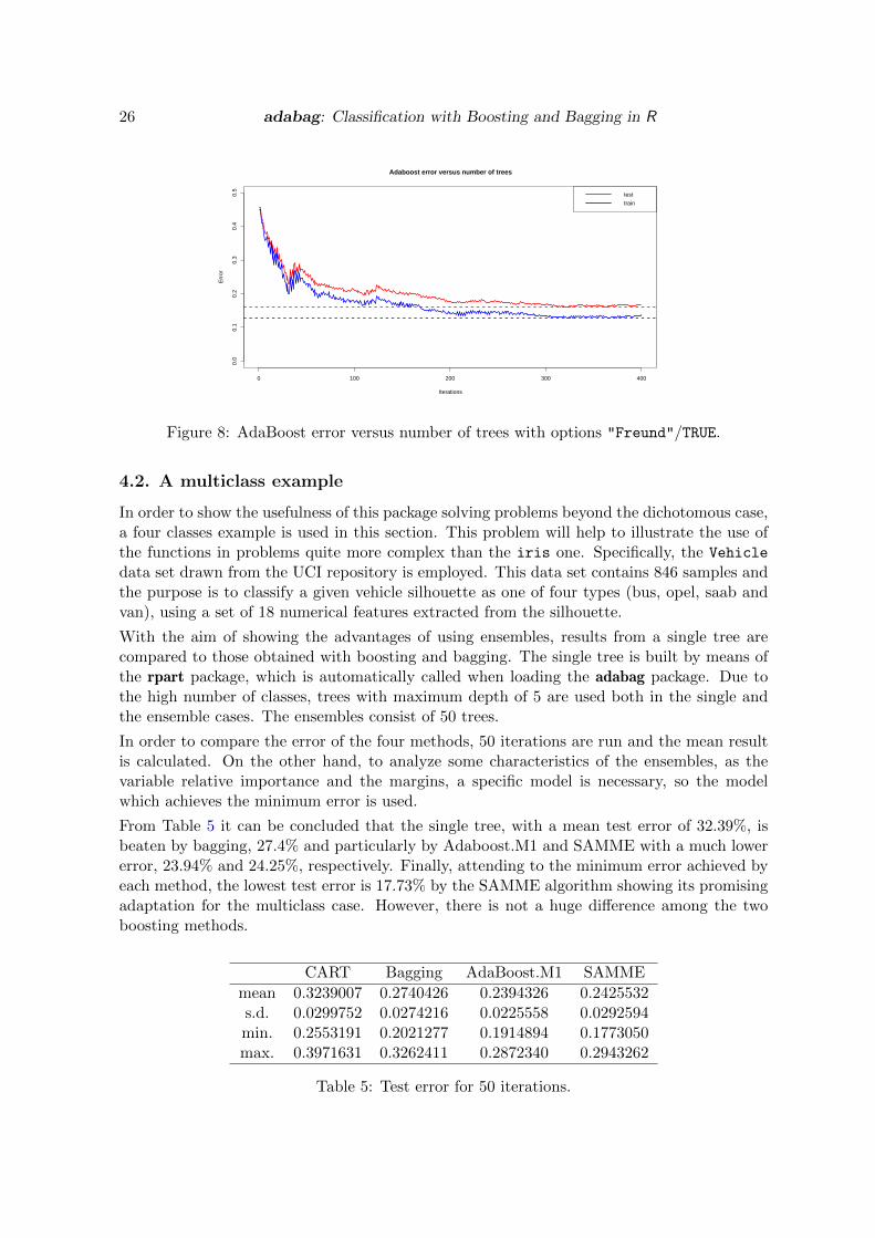
Moreover, Table 4 shows the minimum error achieved along the process and the iterationnumber for which this minimum value has been reached. This is possible thanks to theerrorevol function. The pair Freund-FALSE (Figure 7) achieves the lowest test error and itis worth standing out that this value corresponds nearly to the end of the training process.Thus, it can be reasonably thought that the optimum value has not still been reached. Theevolution of the errors for the four combinations are graphically shown in Figures 5, 6, 7and 8, that are built running the following code for each case.

R> data.boosting <- data.boostingFreundFalse

R> errorevol.train <- errorevol(data.boosting, data[train, ])

R> errorevol.test <- errorevol(data.boosting, data[-train, ])

R> plot(errorevol.test[[1]], type = "l", ylim = c(0, 0.5),

+ main = "Adaboost error versus number of trees", xlab = "Iterations",

+ ylab = "Error", col = "red", lwd = 2)

R> lines(errorevol.train[[1]], cex = 0.5, col = "blue", lty = 1, lwd = 2)

R> legend("topright", c("test", "train"), col = c("red", "blue"), lty = 1,

+ lwd = 2)

R> abline(h = min(errorevol.test[[1]]), col = "red", lty = 2, lwd = 2)

R> abline(h = min(errorevol.train[[1]]), col = "blue", lty = 2, lwd = 2)

The option Breiman/TRUE (Figure 6) achieves its best result much before of the 400-th itera-tion and starts increasing after 253 iterations showing definitely a clear example of overfitting.This can be solved pruning the ensemble as shown next.

R> data.prune <- predict.boosting(data.boosting, newdata = data[-train, ],

+ newmfinal = 253)

R> data.prune$confusion

Observed Class


-1 4347 1040

1 680 3933

R> data.prune$error

[1] 0.172


0 100 200 300 400

0.0

0.1

0.2

0.3

0.4

0.5

Adaboost error versus number of trees

Iterations

Err

ortest

train

Figure 5: AdaBoost error versus number of trees with options "Breiman"/FALSE.

0 100 200 300 400

0.0

0.1

0.2

0.3

0.4

0.5


Iterations

Err

or

test

train

Figure 6: AdaBoost error versus number of trees with options "Breiman"/TRUE.

0 100 200 300 400

0.0

0.1

0.2

0.3

0.4

0.5


Iterations

Err

or

test

train

Figure 7: AdaBoost error versus number of trees with options "Freund"/FALSE.


0 100 200 300 400

0.0

0.1

0.2

0.3

0.4

0.5


Iterations

Err

or

test

train

Figure 8: AdaBoost error versus number of trees with options "Freund"/TRUE.

4.2. A multiclass example

In order to show the usefulness of this package solving problems beyond the dichotomous case,a four classes example is used in this section. This problem will help to illustrate the use ofthe functions in problems quite more complex than the iris one. Specifically, the Vehicle

data set drawn from the UCI repository is employed. This data set contains 846 samples andthe purpose is to classify a given vehicle silhouette as one of four types (bus, opel, saab andvan), using a set of 18 numerical features extracted from the silhouette.

With the aim of showing the advantages of using ensembles, results from a single tree arecompared to those obtained with boosting and bagging. The single tree is built by means ofthe rpart package, which is automatically called when loading the adabag package. Due tothe high number of classes, trees with maximum depth of 5 are used both in the single andthe ensemble cases. The ensembles consist of 50 trees.

In order to compare the error of the four methods, 50 iterations are run and the mean resultis calculated. On the other hand, to analyze some characteristics of the ensembles, as thevariable relative importance and the margins, a specific model is necessary, so the modelwhich achieves the minimum error is used.

From Table 5 it can be concluded that the single tree, with a mean test error of 32.39%, isbeaten by bagging, 27.4% and particularly by Adaboost.M1 and SAMME with a much lowererror, 23.94% and 24.25%, respectively. Finally, attending to the minimum error achieved byeach method, the lowest test error is 17.73% by the SAMME algorithm showing its promisingadaptation for the multiclass case. However, there is not a huge difference among the twoboosting methods.

CART Bagging AdaBoost.M1 SAMME

mean 0.3239007 0.2740426 0.2394326 0.2425532s.d. 0.0299752 0.0274216 0.0225558 0.0292594min. 0.2553191 0.2021277 0.1914894 0.1773050max. 0.3971631 0.3262411 0.2872340 0.2943262

Table 5: Test error for 50 iterations.


R> data("Vehicle")

R> l <- length(Vehicle[ , 1])

R> sub <- sample(1:l, 2 * l/3)

R> maxdepth <- 5

R> Vehicle.rpart <- rpart(Class~., data = Vehicle[sub,], maxdepth = maxdepth)

R> Vehicle.rpart.pred <- predict(Vehicle.rpart, newdata = Vehicle,

+ type = "class")

R> 1 - sum(Vehicle.rpart.pred[sub] == Vehicle$Class[sub]) /

+ length(Vehicle$Class[sub])

[1] 0.2464539

R> tb <- table(Vehicle.rpart.pred[-sub], Vehicle$Class[-sub])

R> tb

bus opel saab van

bus 62 3 3 0

opel 3 26 6 1

saab 3 29 50 5

van 5 5 9 72

R> 1 - sum(Vehicle.rpart.pred[-sub] == Vehicle$Class[-sub]) /

+ length(Vehicle$Class[-sub])

[1] 0.2553191

R> mfinal <- 50

R> cntrl <- rpart.control(maxdepth = 5, minsplit = 0, cp = -1)

R> Vehicle.bagging <- bagging(Class ~ ., data = Vehicle[sub, ],

+ mfinal = mfinal, control = cntrl)

R> 1 - sum(Vehicle.bagging$class == Vehicle$Class[sub]) /


[1] 0.1365248

R> Vehicle.predbagging <- predict.bagging(Vehicle.bagging,

+ newdata = Vehicle[-sub, ])

R> Vehicle.predbagging$confusion

Observed Class

Predicted Class bus opel saab van

bus 68 3 3 0

opel 1 33 9 1

saab 0 31 48 2

van 0 3 4 76

R> Vehicle.predbagging$error


[1] 0.2021277

R> Vehicle.adaboost <- boosting(Class ~., data = Vehicle[sub, ],

+ mfinal = mfinal, coeflearn = "Freund", boos = TRUE, control = cntrl)

R> 1 - sum(Vehicle.adaboost$class == Vehicle$Class[sub])/


[1] 0

R> Vehicle.adaboost.pred <- predict.boosting(Vehicle.adaboost,

+ newdata = Vehicle[-sub,])

R> Vehicle.adaboost.pred$confusion

Observed Class


bus 68 1 0 0

opel 1 41 22 3

saab 0 21 49 0

van 1 3 2 70

R> Vehicle.adaboost.pred$error

[1] 0.1914894

R> Vehicle.SAMME <- boosting(Class ~ ., data = Vehicle[sub, ],

+ mfinal = mfinal, coeflearn = "Zhu", boos = TRUE, control = cntrl)

R> 1 - sum(Vehicle.SAMME$class == Vehicle$Class[sub]) /


[1] 0

R> Vehicle.SAMME.pred <- predict.boosting(Vehicle.SAMME,

+ newdata = Vehicle[-sub, ])

R> Vehicle.SAMME.pred$confusion

Observed Class


bus 71 0 0 0

opel 1 43 24 1

saab 0 21 46 0

van 0 2 1 72

R> Vehicle.SAMME.pred$error

[1] 0.177305


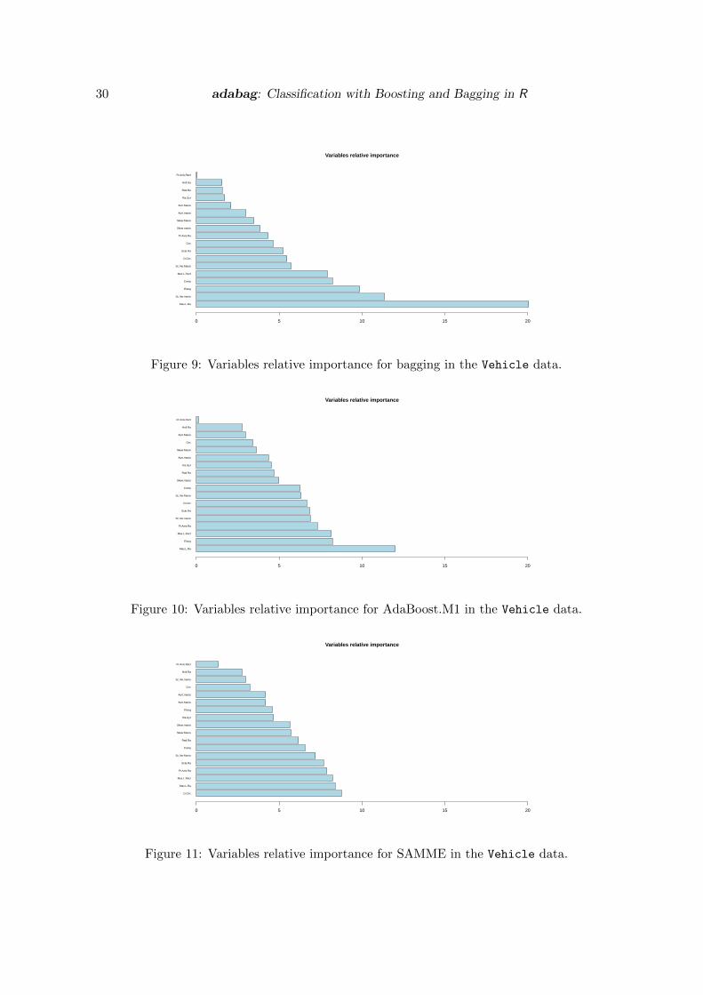
Comparing the relative importance measure for bagging and the two boosting classifiers,they agree in pointing out the two least important variables. The Max.L.Ra has the highestcontribution in bagging and AdaBoost.M1 and the second one for SAMME. Figures 9, 10 and11 show the variables ranked by its relative importance value.

R> sort(Vehicle.bagging$importance, decreasing = TRUE)

Max.L.Ra Sc.Var.maxis Elong Comp Max.L.Rect Sc.Var.Maxis

20.06153052 11.34898853 9.85195343 8.21094638 7.90785330 5.71291406

D.Circ Scat.Ra Circ Pr.Axis.Ra Skew.maxis Skew.Maxis

5.47042335 5.23492044 4.62644012 4.32449318 3.84967772 3.46614732

Kurt.maxis Kurt.Maxis Ra.Gyr Rad.Ra Holl.Ra Pr.Axis.Rect

2.98563804 2.09313159 1.70889907 1.56229729 1.54524768 0.03849798

R> sort(Vehicle.adaboost$importance,decreasing = TRUE)

Max.L.Ra Elong Max.L.Rect Pr.Axis.Ra Sc.Var.maxis Scat.Ra

12.0048265 8.2118048 8.1391111 7.2979696 6.8809291 6.8360291

D.Circ Sc.Var.Maxis Comp Skew.maxis Rad.Ra Ra.Gyr

6.6569366 6.3137727 6.2558542 4.9731790 4.6792429 4.5205229

Kurt.maxis Skew.Maxis Circ Kurt.Maxis Holl.Ra Pr.Axis.Rect

4.3519975 3.6190249 3.4026665 2.9646815 2.7585392 0.1329119

R> sort(Vehicle.SAMME$importance, decreasing = TRUE)

D.Circ Max.L.Ra Max.L.Rect Pr.Axis.Ra Scat.Ra Sc.Var.Maxis

8.759478 8.373885 8.216298 7.869849 7.675569 7.190486

Comp Rad.Ra Skew.Maxis Skew.maxis Ra.Gyr Elong

6.554652 6.158310 5.712122 5.644969 4.652892 4.578929

Kurt.Maxis Kurt.maxis Circ Sc.Var.maxis Holl.Ra Pr.Axis.Rect

4.175756 4.171116 3.223761 2.969842 2.749949 1.322136

R> barplot(sort(Vehicle.bagging$importance, decreasing = TRUE),

+ main = "Variables Relative Importance", col = "lightblue",

+ horiz = TRUE, las = 1, cex.names = .6, xlim = c(0, 20))

Figures 12, 13 and 14 show the cumulative distribution of margins for the bagging and boostingclassifiers developed in this application. The margin of the training set is coloured in blueand the test set in green. For AdaBoost.M1, 19.15% of green negative margins matches thetest error. For SAMME, the blue line is always positive owing to the null training error. Itshould also be pointed out that almost 10% of the observations in bagging, for both sets,achieve the maximum margin equal to 1, which is specially outstanding taking into accountthe large number of classes. To be brief only the code for one of the ensembles is shown herebut all of them are available in the additional file.

R> margins.train <- margins(Vehicle.bagging, Vehicle[sub, ])[[1]]

R> margins.test <- margins(Vehicle.bagging.pred, Vehicle[-sub, ])[[1]]


Max.L.Ra

Sc.Var.maxis

Elong

Comp

Max.L.Rect

Sc.Var.Maxis

D.Circ

Scat.Ra

Circ

Pr.Axis.Ra

Skew.maxis

Skew.Maxis

Kurt.maxis

Kurt.Maxis

Ra.Gyr

Rad.Ra

Holl.Ra

Pr.Axis.Rect


0 5 10 15 20

Figure 9: Variables relative importance for bagging in the Vehicle data.

Max.L.Ra

Elong

Max.L.Rect

Pr.Axis.Ra

Sc.Var.maxis

Scat.Ra

D.Circ

Sc.Var.Maxis

Comp

Skew.maxis

Rad.Ra

Ra.Gyr

Kurt.maxis

Skew.Maxis

Circ

Kurt.Maxis

Holl.Ra

Pr.Axis.Rect


0 5 10 15 20

Figure 10: Variables relative importance for AdaBoost.M1 in the Vehicle data.

D.Circ

Max.L.Ra

Max.L.Rect

Pr.Axis.Ra

Scat.Ra

Sc.Var.Maxis

Comp

Rad.Ra

Skew.Maxis

Skew.maxis

Ra.Gyr

Elong

Kurt.Maxis

Kurt.maxis

Circ

Sc.Var.maxis

Holl.Ra

Pr.Axis.Rect


0 5 10 15 20

Figure 11: Variables relative importance for SAMME in the Vehicle data.


−1.0 −0.5 0.0 0.5 1.0

0.0

0.2

0.4

0.6

0.8

1.0


m

% o

bser

vatio

nstest

train

Figure 12: Margins for bagging in the Vehicle data.

−1.0 −0.5 0.0 0.5 1.0

0.0

0.2

0.4

0.6

0.8

1.0


m

% o

bser

vatio

ns

test

train

Figure 13: Margins for AdaBoost.M1 in the Vehicle data.

−1.0 −0.5 0.0 0.5 1.0

0.0

0.2

0.4

0.6

0.8

1.0


m

% o

bser

vatio

ns

test

train

Figure 14: Margins for SAMME in the Vehicle data.


R> plot(sort(margins.train), (1:length(margins.train)) /

+ length(margins.train), type = "l", xlim = c(-1,1),

+ main = "Margin cumulative distribution graph", xlab = "m",

+ ylab = "% observations", col = "blue3", lty = 2, lwd = 2)

R> abline(v = 0, col = "red", lty = 2, lwd = 2)

R> lines(sort(margins.test), (1:length(margins.test)) / length(margins.test),

+ type = "l", cex = .5, col = "green", lwd = 2)

R> legend("topleft", c("test", "train"), col = c("green", "blue3"),

+ lty = 1:2, lwd = 2)

5. Summary and concluding remarks

In this paper, the R package adabag consisting of eight functions is described. This packageimplements the AdaBoost.M1, SAMME and bagging algorithms with CART trees as baseclassifiers, capable of handling multiclass tasks. The ensemble trained can be used for predic-tion on new data using the generic predict function. Cross validation accuracy estimationscan also be achieved for these classifiers. In addition, the evolution of the error as the en-semble grows can be analysed. This can help to detect overfitting and, on the other hand, ifthe ensemble has not been developed enough and should keep growing. In the former case,the classifier can be pruned without rebuilding it again from the start, selecting a number ofiterations of the current ensemble. Furthermore, not only the predicted class is provided, butalso its margin and an approximation to the probability of all the classes.

The main functionalities of the package are illustrated here by applying them to three well-known datasets from the classification literature. The similarities and differences among thethree algorithms implemented in the package are also discussed. Finally, the addition of someof the plots used here to the package, with the aim of increasing the interpretability of theresults, is part of the future work.

Acknowledgments

The authors are very grateful to the developers of the Vehicle dataset, Pete Mowforth andBarry Shepherd from the Turing Institute, Glasgow, Scotland. Moreover, the authors wouldlike to thank the Editors Jan de Leeuw and Achim Zeileis and two anonymous referees fortheir useful comments and suggestions.

References

Alfaro E, Alfaro JL, Gamez M, Garcıa N (2009). “A Boosting Approach for UnderstandingOut-of-Control Signals in Multivariate Control Charts.” International Journal of ProductionResearch, 47(24), 6821–6834.

Alfaro E, Garcıa N, Gamez M, Elizondo D (2008). “Bankruptcy Forecasting: An EmpiricalComparison of AdaBoost and Neural Networks.” Decission Support Systems, 45, 110–122.


Bache K, Lichman M (2013). “UCI Machine Learning Repository.” URL http://archive.

ics.uci.edu/ml/.

Banfield RE, Hall LO, Bowyer KW, Kegelmeyer WP (2007). “A Comparison of Decision TreeEnsemble Creation Techniques.” IEEE Transactions on Pattern Analysis and MachineIntelligence, 29(1), 173–180.

Bauer E, Kohavi R (1999). “An Empirical Comparison of Voting Classification Algorithm:Bagging, Boosting and Variants.” Machine Learning, 36, 105–139.

Breiman L (1996). “Bagging Predictors.” Machine Learning, 24(2), 123–140.

Breiman L (1998). “Arcing Classifiers.” The Annals of Statistics, 26(3), 801–849.

Breiman L, Friedman JH, Olshenn R, Stone CJ (1984). Classification and Regression Trees.Wadsworth International Group, Belmont.

Buhlmann P, Hothorn T (2007). “Boosting Algorithms: Regularization, Prediction and ModelFitting.” Statistical Science, 22(4), 477–505.

Chrzanowska M, Alfaro E, Witkowska D (2009). “The Individual Borrowers Recognition:Single and Ensemble Trees.” Expert Systems with Applications, 36(3), 6409 – 6414.

Culp M, Johnson K, Michailides G (2006). “ada: An R Package for Stochastic Boosting.”Journal of Statistical Software, 17(2), 1–27. URL http://www.jstatsoft.org/v17/i02/.

Culp M, Johnson K, Michailidis G (2012). ada: An R Package for Stochastic Boosting.R package version 2.0-3, URL http://CRAN.R-project.org/package=ada.

De Bock KW, Coussement K, Van den Poel D (2010). “Ensemble Classification Based onGeneralized Additive Models.” Computational Statistics & Data Analysis, 54(6), 1535–1546.

De Bock KW, Van den Poel D (2011). “An Empirical Valuation of Rotation-Based EnsembleClassifiers for Customer Churn Prediction.” Expert Systems with Applications, 38(10),12293–12301. ISSN 0957–4174.

Dietterich T (2000). “Ensemble Methods in Machine Learning.” In Multiple Classifier Systems,volume 1857 of Lecture Notes in Computer Science, pp. 1–15. Springer-Verlag.

Fan Y, Murphy TB, Watson RWG (2012). digeR: GUI Tool for Analyzing 2D DIGE Data.R package version‘1.3, URL http://CRAN.R-project.org/package=digeR.

Freund Y, Schapire RE (1996). “Experiments with a New Boosting Algorithm.” In L Saitta(ed.), Proceedings of the Thirteenth International Conference on Machine Learning, pp.148–156. Morgan Kaufmann.

Freund Y, Schapire RE (1997). “A Decision-Theoretic Generalization of On-Line Learning andan Application to Boosting.” Journal of Computer and System Sciences, 55(1), 119–139.

Friedman JH, Hastie T, Tibshirani R (2000). “Additive Logistic Regression: A StatisticalView of Boosting.” The Annals of Statistics, 38(2), 337–407.

http://archive.ics.uci.edu/ml/

http://archive.ics.uci.edu/ml/

http://www.jstatsoft.org/v17/i02/

http://CRAN.R-project.org/package=ada

http://CRAN.R-project.org/package=digeR


Hastie T, Tibshirani R, Friedman JH (2001). The Elements of Statistical Learning: DataMining, Inference, and Prediction. Springer-Verlag, New York.

Hothorn T (2013). “CRAN Task View: Machine Learning & Statistical Learning.” Ver-sion 2013-04-18, URL http://CRAN.R-project.org/view=MachineLearning.

Hothorn T, Buhlmann P, Kneib T, Schmid M, Hofner B, Sobotka F, Scheipl F (2013).mboost: Model-Based Boosting. R package version 2.2-2, URL http://CRAN.R-project.

org/package=mboost.

Krempl G, Hofer V (2008). “Partitioner Trees: Combining Boosting and Arbitrating.” InO Okun, G Valentini (eds.), 2nd Workshop SUEMA 2008 (ECAI 2008), pp. 61–66.

Kuhn M (2008). “Building Predictive Models in R Using the caret Package.” Journal ofStatistical Software, 28(5), 1–26. URL http://www.jstatsoft.org/v28/i05/.

Kuhn M (2012). caret: Classification and Regression Training. R package version 5.15-023,URL http://CRAN.R-project.org/package=caret.

Kuncheva LI (2004). Combining Pattern Classifiers: Methods and Algorithms. John Wiley &Sons.

Leisch F, Dimitriadou E (2012). mlbench: Machine Learning Benchmark Problems. R pack-age version 2.1-1, URL http://CRAN.R-project.org/package=mlbench.

Maindonald J, Braun J (2010). Data Analysis and Graphics Using R. 3rd edition. CambridgeUniversity Press.

Mukherjee I, Schapire RE (2011). “A Theory of Multiclass Boosting.” Advances in NeuralInformation Processing Systems, 23(4), 1722–1722.

Opitz DW, Maclin R (1999). “Popular Ensemble Methods: An Empirical Study.” Journal ofArtificial Intelligence Research, 11, 169–198.

R Core Team (2013). R: A Language and Environment for Statistical Computing. R Founda-tion for Statistical Computing, Vienna, Austria. URL http://www.R-project.org/.

Ridgeway G (2013). gbm: Generalized Boosted Regression Models. R package version 2.1,URL http://CRAN.R-project.org/package=gbm.

Schapire RE, Freund Y (2012). Boosting: Foundations and Algorithms. MIT, Cambridge.

Schapire RE, Freund Y, Bartlett P, Lee WS (1998). “Boosting the Margin: A New Explanationfor the Effectiveness of Voting Methods.” The Annals of Statistics, 26, 322–330.

Stewart BM, Zhukov YM (2009). “Use of Force and Civil-Military Relations in Russia: AnAutomated Content Analysis.” Small Wars and Insurgencies, 20(2), 319–343.

Therneau TM, Atkinson B, Ripley BD (2013). rpart: Recursive Partitioning. R packageversion 4.1-1, URL http://CRAN.R-project.org/package=rpart.

Torgo L (2010). Data Mining with R: Learning with Case Studies. Chapman & Hall/CRC.

http://CRAN.R-project.org/view=MachineLearning

http://CRAN.R-project.org/package=mboost

http://CRAN.R-project.org/package=mboost

http://www.jstatsoft.org/v28/i05/

http://CRAN.R-project.org/package=caret

http://CRAN.R-project.org/package=mlbench

http://www.R-project.org/

http://CRAN.R-project.org/package=gbm

http://CRAN.R-project.org/package=rpart


Zhu J, Zou H, Rosset S, Hastie T (2009). “Multi-Class AdaBoost.” Statistics and Its Interface,2, 349–360.

Affiliation:

Esteban Alfaro, Matıas Gamez, Noelia GarcıaFaculty of Economic and Business SciencesUniversity of Castilla-La Mancha02071 Albacete, SpainE-mail: [email protected], [email protected], [email protected]

Journal of Statistical Software http://www.jstatsoft.org/

published by the American Statistical Association http://www.amstat.org/

Volume 54, Issue 2 Submitted: 2012-01-26August 2013 Accepted: 2013-05-29

mailto:[email protected]



http://www.jstatsoft.org/

http://www.amstat.org/

adabag: an r package for classification with boosting … · among the family of boosting...

Documents