boosting and adaboost - university at buffalojcorso/t/cse555/files/lecture... · boosting and...
TRANSCRIPT

Boosting and AdaBoost
Jason Corso
SUNY at Buffalo
J. Corso (SUNY at Buffalo) Boosting and AdaBoost 1 / 62
Introduction
We’ve talked loosely about
1 Lack of inherent superiority of any one particular classifier; and2 Some systematic ways for selecting a particular method over another
for a given scenario.
Now, we turn to boosting and the AdaBoost method for integratingcomponent classifiers into one strong classifier.
J. Corso (SUNY at Buffalo) Boosting and AdaBoost 2 / 62
Introduction
Rationale
Imagine the situation where you want to build an email filter that candistinguish spam from non-spam.
The general way we would approach this problem in ML/PR followsthe same scheme we have for the other topics:
1 Gathering as many examples as possible of both spam and non-spamemails.
2 Train a classifier using these examples and their labels.3 Take the learned classifier, or prediction rule, and use it to filter your
mail.4 The goal is to train a classifier that makes the most accurate
predictions possible on new test examples.And, we’ve covered related topics on how to measure this like bias andvariance.
But, building a highly accurate classifier is a difficult task. (You stillget spam, right?!)
J. Corso (SUNY at Buffalo) Boosting and AdaBoost 3 / 62
Introduction
We could probably come up with many quick rules of thumb. Thesecould be only moderately accurate. Can you think of an example forthis situation?
An example could be “if the subject line contains ‘buy now’ thenclassify as spam.”
This certainly doesn’t cover all spams, but it will be significantlybetter than random guessing.
J. Corso (SUNY at Buffalo) Boosting and AdaBoost 4 / 62
Introduction
Basic Idea of Boosting
Boosting refers to a general and provably effective method ofproducing a very accurate classifier by combining rough andmoderately inaccurate rules of thumb.
It is based on the observation that finding many rough rules ofthumb can be a lot easier than finding a single, highly accurateclassifier.
To begin, we define an algorithm for finding the rules of thumb,which we call a weak learner.
The boosting algorithm repeatedly calls this weak learner, each timefeeding it a different distribution over the training data (in Adaboost).
Each call generates a weak classifier and we must combine all ofthese into a single classifier that, hopefully, is much more accuratethan any one of the rules.
J. Corso (SUNY at Buffalo) Boosting and AdaBoost 5 / 62

Introduction A Toy Example (From Schapire’s Slides)
Toy ExampleToy ExampleToy ExampleToy ExampleToy Example
D1
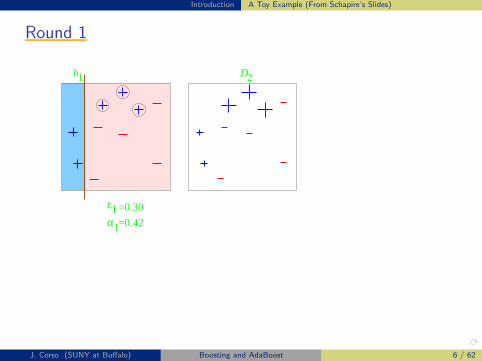
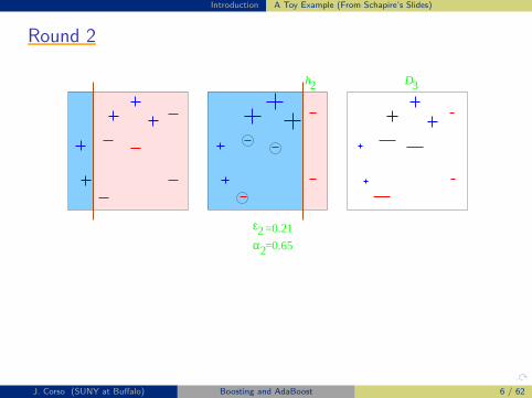
weak classifiers = vertical or horizontal half-planes
J. Corso (SUNY at Buffalo) Boosting and AdaBoost 6 / 62
Introduction A Toy Example (From Schapire’s Slides)
Round 1Round 1Round 1Round 1Round 1
� � � � � � � � � � � �� � � � � � � � � � � �� � � � � � � � � � � �� � � � � � � � � � � �� � � � � � � � � � � �� � � � � � � � � � � �� � � � � � � � � � � �� � � � � � � � � � � �� � � � � � � � � � � �� � � � � � � � � � � �� � � � � � � � � � � �� � � � � � � � � � � �� � � � � � � � � � � �� � � � � � � � � � � �� � � � � � � � � � � �� � � � � � � � � � � �� � � � � � � � � � � �� � � � � � � � � � � �� � � � � � � � � � � �� � � � � � � � � � � �� � � � � � � � � � � �� � � � � � � � � � � �� � � � � � � � � � � �� � � � � � � � � � � �� � � � � � � � � � � �� � � � � � � � � � � �� � � � � � � � � � � �� � � � � � � � � � � �� � � � � � � � � � � �� � � � � � � � � � � �
� � � � � � � � � � � �� � � � � � � � � � � �� � � � � � � � � � � �� � � � � � � � � � � �� � � � � � � � � � � �� � � � � � � � � � � �� � � � � � � � � � � �� � � � � � � � � � � �� � � � � � � � � � � �� � � � � � � � � � � �� � � � � � � � � � � �� � � � � � � � � � � �� � � � � � � � � � � �� � � � � � � � � � � �� � � � � � � � � � � �� � � � � � � � � � � �� � � � � � � � � � � �� � � � � � � � � � � �� � � � � � � � � � � �� � � � � � � � � � � �� � � � � � � � � � � �� � � � � � � � � � � �� � � � � � � � � � � �� � � � � � � � � � � �� � � � � � � � � � � �� � � � � � � � � � � �� � � � � � � � � � � �� � � � � � � � � � � �� � � � � � � � � � � �� � � � � � � � � � � �
� � � �� � � �� � � �� � � �� � � �� � � �� � � �� � � �� � � �� � � �� � � �� � � �� � � �� � � �� � � �� � � �� � � �� � � �� � � �� � � �� � � �� � � �� � � �� � � �� � � �� � � �� � � �� � � �� � � �� � � �
� � � �� � � �� � � �� � � �� � � �� � � �� � � �� � � �� � � �� � � �� � � �� � � �� � � �� � � �� � � �� � � �� � � �� � � �� � � �� � � �� � � �� � � �� � � �� � � �� � � �� � � �� � � �� � � �� � � �� � � �
h1
α
ε1
1
=0.30
=0.42
2D
J. Corso (SUNY at Buffalo) Boosting and AdaBoost 6 / 62
Introduction A Toy Example (From Schapire’s Slides)
Round 2Round 2Round 2Round 2Round 2
� � � � � � � � � � � �� � � � � � � � � � � �� � � � � � � � � � � �� � � � � � � � � � � �� � � � � � � � � � � �� � � � � � � � � � � �� � � � � � � � � � � �� � � � � � � � � � � �� � � � � � � � � � � �� � � � � � � � � � � �� � � � � � � � � � � �� � � � � � � � � � � �� � � � � � � � � � � �� � � � � � � � � � � �� � � � � � � � � � � �� � � � � � � � � � � �� � � � � � � � � � � �� � � � � � � � � � � �� � � � � � � � � � � �� � � � � � � � � � � �� � � � � � � � � � � �� � � � � � � � � � � �� � � � � � � � � � � �� � � � � � � � � � � �� � � � � � � � � � � �� � � � � � � � � � � �� � � � � � � � � � � �� � � � � � � � � � � �� � � � � � � � � � � �� � � � � � � � � � � �
� � � � � � � � � � � �� � � � � � � � � � � �� � � � � � � � � � � �� � � � � � � � � � � �� � � � � � � � � � � �� � � � � � � � � � � �� � � � � � � � � � � �� � � � � � � � � � � �� � � � � � � � � � � �� � � � � � � � � � � �� � � � � � � � � � � �� � � � � � � � � � � �� � � � � � � � � � � �� � � � � � � � � � � �� � � � � � � � � � � �� � � � � � � � � � � �� � � � � � � � � � � �� � � � � � � � � � � �� � � � � � � � � � � �� � � � � � � � � � � �� � � � � � � � � � � �� � � � � � � � � � � �� � � � � � � � � � � �� � � � � � � � � � � �� � � � � � � � � � � �� � � � � � � � � � � �� � � � � � � � � � � �� � � � � � � � � � � �� � � � � � � � � � � �� � � � � � � � � � � �
� � � �� � � �� � � �� � � �� � � �� � � �� � � �� � � �� � � �� � � �� � � �� � � �� � � �� � � �� � � �� � � �� � � �� � � �� � � �� � � �� � � �� � � �� � � �� � � �� � � �� � � �� � � �� � � �� � � �� � � �
� � � �� � � �� � � �� � � �� � � �� � � �� � � �� � � �� � � �� � � �� � � �� � � �� � � �� � � �� � � �� � � �� � � �� � � �� � � �� � � �� � � �� � � �� � � �� � � �� � � �� � � �� � � �� � � �� � � �� � � �
� � � � � � � � � � � � �� � � � � � � � � � � � �� � � � � � � � � � � � �� � � � � � � � � � � � �� � � � � � � � � � � � �� � � � � � � � � � � � �� � � � � � � � � � � � �� � � � � � � � � � � � �� � � � � � � � � � � � �� � � � � � � � � � � � �� � � � � � � � � � � � �� � � � � � � � � � � � �� � � � � � � � � � � � �� � � � � � � � � � � � �� � � � � � � � � � � � �� � � � � � � � � � � � �� � � � � � � � � � � � �� � � � � � � � � � � � �� � � � � � � � � � � � �� � � � � � � � � � � � �� � � � � � � � � � � � �� � � � � � � � � � � � �� � � � � � � � � � � � �� � � � � � � � � � � � �� � � � � � � � � � � � �� � � � � � � � � � � � �� � � � � � � � � � � � �� � � � � � � � � � � � �� � � � � � � � � � � � �� � � � � � � � � � � � �
� � � �� � � �� � � �� � � �� � � �� � � �� � � �� � � �� � � �� � � �� � � �� � � �� � � �� � � �� � � �� � � �� � � �� � � �� � � �� � � �� � � �� � � �� � � �� � � �� � � �� � � �� � � �� � � �� � � �� � � �
α
ε2
2
=0.21
=0.65
h2 3D
J. Corso (SUNY at Buffalo) Boosting and AdaBoost 6 / 62

Introduction A Toy Example (From Schapire’s Slides)
Round 3Round 3Round 3Round 3Round 3
� � � �� � � �� � � �� � � �� � � �� � � �� � � �� � � �� � � �� � � �� � � �� � � �� � � �� � � �� � � �� � � �� � � �� � � �� � � �� � � �� � � �� � � �� � � �� � � �� � � �� � � �� � � �� � � �� � � �� � � �
� � � � � � � � � � � � �� � � � � � � � � � � � �� � � � � � � � � � � � �� � � � � � � � � � � � �� � � � � � � � � � � � �� � � � � � � � � � � � �� � � � � � � � � � � � �� � � � � � � � � � � � �� � � � � � � � � � � � �� � � � � � � � � � � � �� � � � � � � � � � � � �� � � � � � � � � � � � �� � � � � � � � � � � � �� � � � � � � � � � � � �� � � � � � � � � � � � �� � � � � � � � � � � � �� � � � � � � � � � � � �� � � � � � � � � � � � �� � � � � � � � � � � � �� � � � � � � � � � � � �� � � � � � � � � � � � �� � � � � � � � � � � � �� � � � � � � � � � � � �� � � � � � � � � � � � �� � � � � � � � � � � � �� � � � � � � � � � � � �� � � � � � � � � � � � �� � � � � � � � � � � � �� � � � � � � � � � � � �� � � � � � � � � � � � �
� � � � � � � � � � � � �� � � � � � � � � � � � �� � � � � � � � � � � � �� � � � � � � � � � � � �� � � � � � � � � � � � �� � � � � � � � � � � � �� � � � � � � � � � � � �� � � � � � � � � � � � �� � � � � � � � � � � � �� � � � � � � � � � � � �� � � � � � � � � � � � �� � � � � � � � � � � � �� � � � � � � � � � � � �� � � � � � � � � � � � �� � � � � � � � � � � � �� � � � � � � � � � � � �� � � � � � � � � � � � �� � � � � � � � � � � � �� � � � � � � � � � � � �� � � � � � � � � � � � �� � � � � � � � � � � � �� � � � � � � � � � � � �� � � � � � � � � � � � �� � � � � � � � � � � � �� � � � � � � � � � � � �� � � � � � � � � � � � �� � � � � � � � � � � � �� � � � � � � � � � � � �� � � � � � � � � � � � �� � � � � � � � � � � � �
� � � �� � � �� � � �� � � �� � � �� � � �� � � �� � � �� � � �� � � �� � � �� � � �� � � �� � � �� � � �� � � �� � � �� � � �� � � �� � � �� � � �� � � �� � � �� � � �� � � �� � � �� � � �� � � �� � � �� � � �
� � � �� � � �� � � �� � � �� � � �� � � �� � � �� � � �� � � �� � � �� � � �� � � �� � � �� � � �� � � �� � � �� � � �� � � �� � � �� � � �� � � �� � � �� � � �� � � �� � � �� � � �� � � �� � � �� � � �� � � �
� � � � � � � � � � � �� � � � � � � � � � � �� � � � � � � � � � � �� � � � � � � � � � � �� � � � � � � � � � � �� � � � � � � � � � � �� � � � � � � � � � � �� � � � � � � � � � � �� � � � � � � � � � � �� � � � � � � � � � � �� � � � � � � � � � � �� � � � � � � � � � � �� � � � � � � � � � � �� � � � � � � � � � � �� � � � � � � � � � � �� � � � � � � � � � � �� � � � � � � � � � � �� � � � � � � � � � � �� � � � � � � � � � � �� � � � � � � � � � � �� � � � � � � � � � � �� � � � � � � � � � � �� � � � � � � � � � � �� � � � � � � � � � � �� � � � � � � � � � � �� � � � � � � � � � � �� � � � � � � � � � � �� � � � � � � � � � � �� � � � � � � � � � � �� � � � � � � � � � � �
� � � � � � � � � � � �� � � � � � � � � � � �� � � � � � � � � � � �� � � � � � � � � � � �� � � � � � � � � � � �� � � � � � � � � � � �� � � � � � � � � � � �� � � � � � � � � � � �� � � � � � � � � � � �� � � � � � � � � � � �� � � � � � � � � � � �� � � � � � � � � � � �� � � � � � � � � � � �� � � � � � � � � � � �� � � � � � � � � � � �� � � � � � � � � � � �� � � � � � � � � � � �� � � � � � � � � � � �� � � � � � � � � � � �� � � � � � � � � � � �� � � � � � � � � � � �� � � � � � � � � � � �� � � � � � � � � � � �� � � � � � � � � � � �� � � � � � � � � � � �� � � � � � � � � � � �� � � � � � � � � � � �� � � � � � � � � � � �� � � � � � � � � � � �� � � � � � � � � � � �
� � � � � � � � � � � � � � � �� � � � � � � � � � � � � � � �� � � � � � � � � � � � � � � �� � � � � � � � � � � � � � � �� � � � � � � � � � � � � � � �� � � � � � � � � � � � � � � �� � � � � � � � � � � � � � � �� � � � � � � � � � � � � � � �� � � � � � � � � � � � � � � �� � � � � � � � � � � � � � � �� � � � � � � � � � � � � � � �� � � � � � � � � � � � � � � �� � � � � � � � � � � � � � � �� � � � � � � � � � � � � � � �� � � � � � � � � � � � � � � �� � � � � � � � � � � � � � � �� � � � � � � � � � � � � � � �� � � � � � � � � � � � � � � �� � � � � � � � � � � � � � � �� � � � � � � � � � � � � � � �� � � � � � � � � � � � � � � �� � � � � � � � � � � � � � � �
� � � � � � � � � � � � � � � �� � � � � � � � � � � � � � � �� � � � � � � � � � � � � � � �� � � � � � � � � � � � � � � �� � � � � � � � � � � � � � � �� � � � � � � � � � � � � � � �� � � � � � � � � � � � � � � �� � � � � � � � � � � � � � � �� � � � � � � � � � � � � � � �� � � � � � � � � � � � � � � �� � � � � � � � � � � � � � � �� � � � � � � � � � � � � � � �� � � � � � � � � � � � � � � �� � � � � � � � � � � � � � � �� � � � � � � � � � � � � � � �� � � � � � � � � � � � � � � �� � � � � � � � � � � � � � � �� � � � � � � � � � � � � � � �� � � � � � � � � � � � � � � �� � � � � � � � � � � � � � � �� � � � � � � � � � � � � � � �� � � � � � � � � � � � � � � �� � � � � � � � � � � � � � � �� � � � � � � � � � � � � � � �� � � � � � � � � � � � � � � �� � � � � � � � � � � � � � � �� � � � � � � � � � � � � � � �� � � � � � � � � � � � � � � �� � � � � � � � � � � � � � � �� � � � � � � � � � � � � � � �� � � � � � � � � � � � � � � �� � � � � � � � � � � � � � � �
� � � � � � � � � � � � � � � �� � � � � � � � � � � � � � � �� � � � � � � � � � � � � � � �� � � � � � � � � � � � � � � �� � � � � � � � � � � � � � � �� � � � � � � � � � � � � � � �� � � � � � � � � � � � � � � �� � � � � � � � � � � � � � � �� � � � � � � � � � � � � � � �� � � � � � � � � � � � � � � �
h3
α
ε3
3=0.92
=0.14
J. Corso (SUNY at Buffalo) Boosting and AdaBoost 6 / 62

Introduction A Toy Example (From Schapire’s Slides)
Final ClassifierFinal ClassifierFinal ClassifierFinal ClassifierFinal Classifier
� � � � � � � �� � � � � � � �� � � � � � � �� � � � � � � �� � � � � � � �� � � � � � � �� � � � � � � �� � � � � � � �� � � � � � � �� � � � � � � �� � � � � � � �� � � � � � � �� � � � � � � �� � � � � � � �� � � � � � � �� � � � � � � �� � � � � � � �� � � � � � � �� � � � � � � �
� � � � � � � �� � � � � � � �� � � � � � � �� � � � � � � �� � � � � � � �� � � � � � � �� � � � � � � �� � � � � � � �� � � � � � � �� � � � � � � �� � � � � � � �� � � � � � � �� � � � � � � �� � � � � � � �� � � � � � � �� � � � � � � �� � � � � � � �� � � � � � � �� � � � � � � �
� � � �� � � �� � � �� � � �� � � �� � � �� � � �� � � �� � � �� � � �� � � �� � � �� � � �� � � �� � � �� � � �� � � �� � � �� � � �� � � �� � � �� � � �� � � �� � � �� � � �� � � �� � � �� � � �� � � �� � � �� � � �
� � � �� � � �� � � �� � � �� � � �� � � �� � � �� � � �� � � �� � � �� � � �� � � �� � � �� � � �� � � �� � � �� � � �� � � �� � � �� � � �� � � �� � � �� � � �� � � �� � � �� � � �� � � �� � � �� � � �� � � �� � � �
� � � � � � � � � � �� � � � � � � � � � �� � � � � � � � � � �� � � � � � � � � � �� � � � � � � � � � �� � � � � � � � � � �� � � � � � � � � � �
� � � � � � � � � � �� � � � � � � � � � �� � � � � � � � � � �� � � � � � � � � � �� � � � � � � � � � �� � � � � � � � � � �� � � � � � � � � � �
� � � � � � � � � � �� � � � � � � � � � �� � � � � � � � � � �� � � � � � � � � � �� � � � � � � � � � �� � � � � � � � � � �� � � � � � � � � � �� � � � � � � � � � �� � � � � � � � � � �� � � � � � � � � � �� � � � � � � � � � �� � � � � � � � � � �� � � � � � � � � � �
� � � � � � � � � � �� � � � � � � � � � �� � � � � � � � � � �� � � � � � � � � � �� � � � � � � � � � �� � � � � � � � � � �� � � � � � � � � � �� � � � � � � � � � �� � � � � � � � � � �� � � � � � � � � � �� � � � � � � � � � �� � � � � � � � � � �� � � � � � � � � � �
! !! !! !! !! !! !! !! !! !! !! !! !! !! !! !! !! !! !! !
" " " " " " " " " " " " "" " " " " " " " " " " " "" " " " " " " " " " " " "" " " " " " " " " " " " "" " " " " " " " " " " " "" " " " " " " " " " " " "" " " " " " " " " " " " "" " " " " " " " " " " " "" " " " " " " " " " " " "" " " " " " " " " " " " "" " " " " " " " " " " " "" " " " " " " " " " " " "" " " " " " " " " " " " "" " " " " " " " " " " " "" " " " " " " " " " " " "" " " " " " " " " " " " "" " " " " " " " " " " " "" " " " " " " " " " " " "" " " " " " " " " " " " "" " " " " " " " " " " " "" " " " " " " " " " " " "" " " " " " " " " " " " "" " " " " " " " " " " " "" " " " " " " " " " " " "" " " " " " " " " " " " "" " " " " " " " " " " " "" " " " " " " " " " " " "" " " " " " " " " " " " "" " " " " " " " " " " " "" " " " " " " " " " " " "" " " " " " " " " " " " "
# # # # # # # # # # # ## # # # # # # # # # # ## # # # # # # # # # # ## # # # # # # # # # # ## # # # # # # # # # # ## # # # # # # # # # # ## # # # # # # # # # # ## # # # # # # # # # # ## # # # # # # # # # # ## # # # # # # # # # # ## # # # # # # # # # # ## # # # # # # # # # # ## # # # # # # # # # # ## # # # # # # # # # # ## # # # # # # # # # # ## # # # # # # # # # # ## # # # # # # # # # # ## # # # # # # # # # # ## # # # # # # # # # # ## # # # # # # # # # # ## # # # # # # # # # # ## # # # # # # # # # # ## # # # # # # # # # # ## # # # # # # # # # # ## # # # # # # # # # # ## # # # # # # # # # # ## # # # # # # # # # # ## # # # # # # # # # # ## # # # # # # # # # # ## # # # # # # # # # # ## # # # # # # # # # # #
$ $ $ $ $ $ $ $ $$ $ $ $ $ $ $ $ $$ $ $ $ $ $ $ $ $$ $ $ $ $ $ $ $ $$ $ $ $ $ $ $ $ $$ $ $ $ $ $ $ $ $$ $ $ $ $ $ $ $ $$ $ $ $ $ $ $ $ $$ $ $ $ $ $ $ $ $$ $ $ $ $ $ $ $ $$ $ $ $ $ $ $ $ $$ $ $ $ $ $ $ $ $$ $ $ $ $ $ $ $ $$ $ $ $ $ $ $ $ $$ $ $ $ $ $ $ $ $$ $ $ $ $ $ $ $ $$ $ $ $ $ $ $ $ $$ $ $ $ $ $ $ $ $$ $ $ $ $ $ $ $ $
% % % % % % % % %% % % % % % % % %% % % % % % % % %% % % % % % % % %% % % % % % % % %% % % % % % % % %% % % % % % % % %% % % % % % % % %% % % % % % % % %% % % % % % % % %% % % % % % % % %% % % % % % % % %% % % % % % % % %% % % % % % % % %% % % % % % % % %% % % % % % % % %% % % % % % % % %% % % % % % % % %% % % % % % % % %
& && && && && && && && && && && && && && && && && && && &
' '' '' '' '' '' '' '' '' '' '' '' '' '' '' '' '' '' '' '
( ( ( ( ( ( ( ( ( ( ( (( ( ( ( ( ( ( ( ( ( ( (( ( ( ( ( ( ( ( ( ( ( (( ( ( ( ( ( ( ( ( ( ( (( ( ( ( ( ( ( ( ( ( ( (( ( ( ( ( ( ( ( ( ( ( (( ( ( ( ( ( ( ( ( ( ( (( ( ( ( ( ( ( ( ( ( ( (( ( ( ( ( ( ( ( ( ( ( (( ( ( ( ( ( ( ( ( ( ( (
) ) ) ) ) ) ) ) ) ) ) )) ) ) ) ) ) ) ) ) ) ) )) ) ) ) ) ) ) ) ) ) ) )) ) ) ) ) ) ) ) ) ) ) )) ) ) ) ) ) ) ) ) ) ) )) ) ) ) ) ) ) ) ) ) ) )) ) ) ) ) ) ) ) ) ) ) )) ) ) ) ) ) ) ) ) ) ) )) ) ) ) ) ) ) ) ) ) ) )) ) ) ) ) ) ) ) ) ) ) )
Hfinal
+ 0.92+ 0.650.42sign=
=
J. Corso (SUNY at Buffalo) Boosting and AdaBoost 6 / 62

Introduction A Toy Example (From Schapire’s Slides)
STOP!
J. Corso (SUNY at Buffalo) Boosting and AdaBoost 7 / 62

Introduction Introduction Wrap-Up
Key Questions Defining and Analyzing Boosting
1 How should the distribution be chosen each round?
2 How should the weak rules be combined into a single rule?
3 How should the weak learner be defined?
4 How many weak classifiers should we learn?
J. Corso (SUNY at Buffalo) Boosting and AdaBoost 8 / 62

Basic AdaBoost
Getting Started
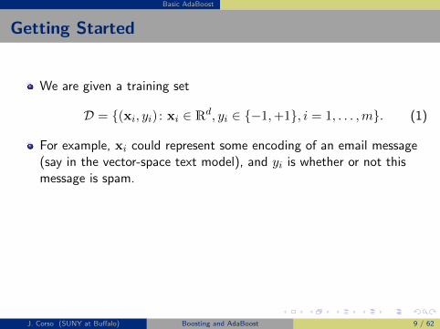
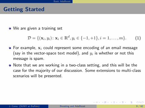
We are given a training set
D = {(xi, yi) : xi ∈ Rd, yi ∈ {−1,+1}, i = 1, . . . ,m}. (1)
For example, xi could represent some encoding of an email message(say in the vector-space text model), and yi is whether or not thismessage is spam.
Note that we are working in a two-class setting, and this will be thecase for the majority of our discussion. Some extensions to multi-classscenarios will be presented.
We need to define a distribution D over the dataset D such that∑iD(i) = 1.
J. Corso (SUNY at Buffalo) Boosting and AdaBoost 9 / 62
Basic AdaBoost
Getting Started
We are given a training set
D = {(xi, yi) : xi ∈ Rd, yi ∈ {−1,+1}, i = 1, . . . ,m}. (1)
For example, xi could represent some encoding of an email message(say in the vector-space text model), and yi is whether or not thismessage is spam.
Note that we are working in a two-class setting, and this will be thecase for the majority of our discussion. Some extensions to multi-classscenarios will be presented.
We need to define a distribution D over the dataset D such that∑iD(i) = 1.
J. Corso (SUNY at Buffalo) Boosting and AdaBoost 9 / 62
Basic AdaBoost Weak Learners and Weak Classifiers
Weak Learners and Weak Classifiers
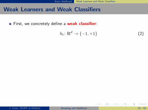
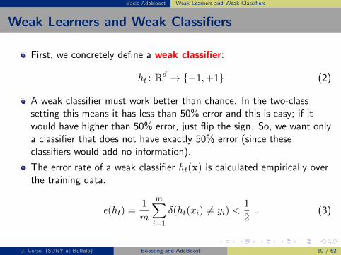
First, we concretely define a weak classifier:
ht : Rd → {−1,+1} (2)
A weak classifier must work better than chance. In the two-classsetting this means it has less than 50% error and this is easy; if itwould have higher than 50% error, just flip the sign. So, we want onlya classifier that does not have exactly 50% error (since theseclassifiers would add no information).
The error rate of a weak classifier ht(x) is calculated empirically overthe training data:
ε(ht) =1
m
m∑i=1
δ(ht(xi) 6= yi) <1
2. (3)
J. Corso (SUNY at Buffalo) Boosting and AdaBoost 10 / 62

Basic AdaBoost Weak Learners and Weak Classifiers
Weak Learners and Weak Classifiers
First, we concretely define a weak classifier:
ht : Rd → {−1,+1} (2)
A weak classifier must work better than chance. In the two-classsetting this means it has less than 50% error and this is easy; if itwould have higher than 50% error, just flip the sign. So, we want onlya classifier that does not have exactly 50% error (since theseclassifiers would add no information).
The error rate of a weak classifier ht(x) is calculated empirically overthe training data:
ε(ht) =1
m
m∑i=1
δ(ht(xi) 6= yi) <1
2. (3)
J. Corso (SUNY at Buffalo) Boosting and AdaBoost 10 / 62
Basic AdaBoost Weak Learners and Weak Classifiers
A WL/WC Example for Images
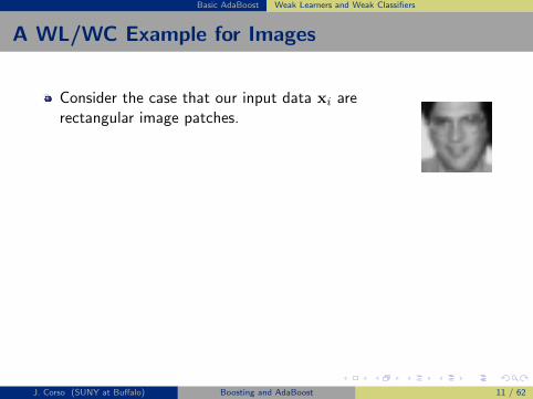
Consider the case that our input data xi arerectangular image patches.
Given example images where
for negative and positive examples respec-
tively.
Initialize weights for respec-
tively, where and are the number of negatives and
positives respectively.
For :
1. Normalize the weights,
so that is a probability distribution.
2. For each feature, , train a classifi er which
is restricted to using a single feature. The
error is evaluated with respect to ,
.
3. Choose the classifi er, , with the lowest error .
4. Update the weights:
where if example is classifi ed cor-
rectly, otherwise, and .
The fi nal strong classifi er is:
otherwise
where
Table 1: The AdaBoost algorithm for classifier learn-
ing. Each round of boosting selects one feature from the
180,000 potential features.
number of features are retained (perhaps a few hundred or
thousand).
3.2. Learning Results
While details on the training and performance of the final
system are presented in Section 5, several simple results
merit discussion. Initial experiments demonstrated that a
frontal face classifier constructed from 200 features yields
a detection rate of 95% with a false positive rate of 1 in
14084. These results are compelling, but not sufficient for
many real-world tasks. In terms of computation, this clas-
sifier is probably faster than any other published system,
requiring 0.7 seconds to scan an 384 by 288 pixel image.
Unfortunately, the most straightforward technique for im-
proving detection performance, adding features to the clas-
sifier, directly increases computation time.
For the task of face detection, the initial rectangle fea-
tures selected by AdaBoost are meaningful and easily inter-
preted. The first feature selected seems to focus on the prop-
erty that the region of the eyes is often darker than the region
Figure 3: The first and second features selected by Ad-
aBoost. The two features are shown in the top row and then
overlayed on a typical training face in the bottom row. The
first feature measures the difference in intensity between the
region of the eyes and a region across the upper cheeks. The
feature capitalizes on the observation that the eye region is
often darker than the cheeks. The second feature compares
the intensities in the eye regions to the intensity across the
bridge of the nose.
of the nose and cheeks (see Figure 3). This feature is rel-
atively large in comparison with the detection sub-window,
and should be somewhat insensitive to size and location of
the face. The second feature selected relies on the property
that the eyes are darker than the bridge of the nose.
4. The Attentional Cascade
This section describes an algorithm for constructing a cas-
cade of classifiers which achieves increased detection per-
formance while radically reducing computation time. The
key insight is that smaller, and therefore more efficient,
boosted classifiers can be constructed which reject many of
the negative sub-windows while detecting almost all posi-
tive instances (i.e. the threshold of a boosted classifier can
be adjusted so that the false negative rate is close to zero).
Simpler classifiers are used to reject the majority of sub-
windows before more complex classifiers are called upon
to achieve low false positive rates.
The overall form of the detection process is that of a de-
generate decision tree, what we call a “cascade” (see Fig-
ure 4). A positive result from the first classifier triggers the
evaluation of a second classifier which has also been ad-
justed to achieve very high detection rates. A positive result
from the second classifier triggers a third classifier, and so
on. A negative outcome at any point leads to the immediate
rejection of the sub-window.
Stages in the cascade are constructed by training clas-
sifiers using AdaBoost and then adjusting the threshold to
minimize false negatives. Note that the default AdaBoost
threshold is designed to yield a low error rate on the train-
ing data. In general a lower threshold yields higher detec-
4
Define a collection of Haar-likerectangle features.
The feature value extracted isthe difference of the pixel sumin the white sub-regions and theblack sub-regions.
With a base patch size of 24x24,there are over 180,000 possiblesuch rectangle features.
single feature [2]. As a result each stage of the boosting
process, which selects a new weak classifier, can be viewed
as a feature selection process. AdaBoost provides an effec-
tive learning algorithm and strong bounds on generalization
performance [13, 9, 10].
The third major contribution of this paper is a method
for combining successively more complex classifiers in a
cascade structure which dramatically increases the speed of
the detector by focusing attention on promising regions of
the image. The notion behind focus of attention approaches
is that it is often possible to rapidly determine where in an
image an object might occur [17, 8, 1]. More complex pro-
cessing is reserved only for these promising regions. The
key measure of such an approach is the “false negative” rate
of the attentional process. It must be the case that all, or
almost all, object instances are selected by the attentional
filter.
We will describe a process for training an extremely sim-
ple and efficient classifier which can be used as a “super-
vised” focus of attention operator. The term supervised
refers to the fact that the attentional operator is trained to
detect examples of a particular class. In the domain of face
detection it is possible to achieve fewer than 1% false neg-
atives and 40% false positives using a classifier constructed
from two Harr-like features. The effect of this filter is to
reduce by over one half the number of locations where the
final detector must be evaluated.
Those sub-windows which are not rejected by the initial
classifier are processed by a sequence of classifiers, each
slightly more complex than the last. If any classifier rejects
the sub-window, no further processing is performed. The
structure of the cascaded detection process is essentially
that of a degenerate decision tree, and as such is related to
the work of Geman and colleagues [1, 4].
An extremely fast face detector will have broad prac-
tical applications. These include user interfaces, image
databases, and teleconferencing. In applications where
rapid frame-rates are not necessary, our system will allow
for significant additional post-processing and analysis. In
addition our system can be implemented on a wide range of
small low power devices, including hand-helds and embed-
ded processors. In our lab we have implemented this face
detector on the Compaq iPaq handheld and have achieved
detection at two frames per second (this device has a low
power 200 mips Strong Arm processor which lacks floating
point hardware).
The remainder of the paper describes our contributions
and a number of experimental results, including a detailed
description of our experimental methodology. Discussion
of closely related work takes place at the end of each sec-
tion.
2. Features
Our object detection procedure classifies images based on
the value of simple features. There are many motivations
A B
C D
Figure 1: Example rectangle features shown relative to the
enclosing detection window. The sum of the pixels which
lie within the white rectangles are subtracted from the sum
of pixels in the grey rectangles. Two-rectangle features are
shown in (A) and (B). Figure (C) shows a three-rectangle
feature, and (D) a four-rectangle feature.
for using features rather than the pixels directly. The most
common reason is that features can act to encode ad-hoc
domain knowledge that is difficult to learn using a finite
quantity of training data. For this system there is also a
second critical motivation for features: the feature based
system operates much faster than a pixel-based system.
The simple features used are reminiscent of Haar basis
functions which have been used by Papageorgiou et al. [10].
More specifically, we use three kinds of features. The value
of a two-rectangle feature is the difference between the sum
of the pixels within two rectangular regions. The regions
have the same size and shape and are horizontally or ver-
tically adjacent (see Figure 1). A three-rectangle feature
computes the sum within two outside rectangles subtracted
from the sum in a center rectangle. Finally a four-rectangle
feature computes the difference between diagonal pairs of
rectangles.
Given that the base resolution of the detector is 24x24,
the exhaustive set of rectangle features is quite large, over
180,000 . Note that unlike the Haar basis, the set of rectan-
gle features is overcomplete1.
2.1. Integral Image
Rectangle features can be computed very rapidly using an
intermediate representation for the image which we call the
integral image.2 The integral image at location contains
the sum of the pixels above and to the left of , inclusive:
1A complete basis has no linear dependence between basis elements
and has the same number of elements as the image space, in this case 576.
The full set of 180,000 thousand features is many times over-complete.2There is a close relation to “summed area tables” as used in graphics
[3]. We choose a different name here in order to emphasize its use for the
analysis of images, rather than for texture mapping.
2
J. Corso (SUNY at Buffalo) Boosting and AdaBoost 11 / 62

Basic AdaBoost Weak Learners and Weak Classifiers
A WL/WC Example for Images
Consider the case that our input data xi arerectangular image patches.
Given example images where
for negative and positive examples respec-
tively.
Initialize weights for respec-
tively, where and are the number of negatives and
positives respectively.
For :
1. Normalize the weights,
so that is a probability distribution.
2. For each feature, , train a classifi er which
is restricted to using a single feature. The
error is evaluated with respect to ,
.
3. Choose the classifi er, , with the lowest error .
4. Update the weights:
where if example is classifi ed cor-
rectly, otherwise, and .
The fi nal strong classifi er is:
otherwise
where
Table 1: The AdaBoost algorithm for classifier learn-
ing. Each round of boosting selects one feature from the
180,000 potential features.
number of features are retained (perhaps a few hundred or
thousand).
3.2. Learning Results
While details on the training and performance of the final
system are presented in Section 5, several simple results
merit discussion. Initial experiments demonstrated that a
frontal face classifier constructed from 200 features yields
a detection rate of 95% with a false positive rate of 1 in
14084. These results are compelling, but not sufficient for
many real-world tasks. In terms of computation, this clas-
sifier is probably faster than any other published system,
requiring 0.7 seconds to scan an 384 by 288 pixel image.
Unfortunately, the most straightforward technique for im-
proving detection performance, adding features to the clas-
sifier, directly increases computation time.
For the task of face detection, the initial rectangle fea-
tures selected by AdaBoost are meaningful and easily inter-
preted. The first feature selected seems to focus on the prop-
erty that the region of the eyes is often darker than the region
Figure 3: The first and second features selected by Ad-
aBoost. The two features are shown in the top row and then
overlayed on a typical training face in the bottom row. The
first feature measures the difference in intensity between the
region of the eyes and a region across the upper cheeks. The
feature capitalizes on the observation that the eye region is
often darker than the cheeks. The second feature compares
the intensities in the eye regions to the intensity across the
bridge of the nose.
of the nose and cheeks (see Figure 3). This feature is rel-
atively large in comparison with the detection sub-window,
and should be somewhat insensitive to size and location of
the face. The second feature selected relies on the property
that the eyes are darker than the bridge of the nose.
4. The Attentional Cascade
This section describes an algorithm for constructing a cas-
cade of classifiers which achieves increased detection per-
formance while radically reducing computation time. The
key insight is that smaller, and therefore more efficient,
boosted classifiers can be constructed which reject many of
the negative sub-windows while detecting almost all posi-
tive instances (i.e. the threshold of a boosted classifier can
be adjusted so that the false negative rate is close to zero).
Simpler classifiers are used to reject the majority of sub-
windows before more complex classifiers are called upon
to achieve low false positive rates.
The overall form of the detection process is that of a de-
generate decision tree, what we call a “cascade” (see Fig-
ure 4). A positive result from the first classifier triggers the
evaluation of a second classifier which has also been ad-
justed to achieve very high detection rates. A positive result
from the second classifier triggers a third classifier, and so
on. A negative outcome at any point leads to the immediate
rejection of the sub-window.
Stages in the cascade are constructed by training clas-
sifiers using AdaBoost and then adjusting the threshold to
minimize false negatives. Note that the default AdaBoost
threshold is designed to yield a low error rate on the train-
ing data. In general a lower threshold yields higher detec-
4
Define a collection of Haar-likerectangle features.
The feature value extracted isthe difference of the pixel sumin the white sub-regions and theblack sub-regions.
With a base patch size of 24x24,there are over 180,000 possiblesuch rectangle features.
single feature [2]. As a result each stage of the boosting
process, which selects a new weak classifier, can be viewed
as a feature selection process. AdaBoost provides an effec-
tive learning algorithm and strong bounds on generalization
performance [13, 9, 10].
The third major contribution of this paper is a method
for combining successively more complex classifiers in a
cascade structure which dramatically increases the speed of
the detector by focusing attention on promising regions of
the image. The notion behind focus of attention approaches
is that it is often possible to rapidly determine where in an
image an object might occur [17, 8, 1]. More complex pro-
cessing is reserved only for these promising regions. The
key measure of such an approach is the “false negative” rate
of the attentional process. It must be the case that all, or
almost all, object instances are selected by the attentional
filter.
We will describe a process for training an extremely sim-
ple and efficient classifier which can be used as a “super-
vised” focus of attention operator. The term supervised
refers to the fact that the attentional operator is trained to
detect examples of a particular class. In the domain of face
detection it is possible to achieve fewer than 1% false neg-
atives and 40% false positives using a classifier constructed
from two Harr-like features. The effect of this filter is to
reduce by over one half the number of locations where the
final detector must be evaluated.
Those sub-windows which are not rejected by the initial
classifier are processed by a sequence of classifiers, each
slightly more complex than the last. If any classifier rejects
the sub-window, no further processing is performed. The
structure of the cascaded detection process is essentially
that of a degenerate decision tree, and as such is related to
the work of Geman and colleagues [1, 4].
An extremely fast face detector will have broad prac-
tical applications. These include user interfaces, image
databases, and teleconferencing. In applications where
rapid frame-rates are not necessary, our system will allow
for significant additional post-processing and analysis. In
addition our system can be implemented on a wide range of
small low power devices, including hand-helds and embed-
ded processors. In our lab we have implemented this face
detector on the Compaq iPaq handheld and have achieved
detection at two frames per second (this device has a low
power 200 mips Strong Arm processor which lacks floating
point hardware).
The remainder of the paper describes our contributions
and a number of experimental results, including a detailed
description of our experimental methodology. Discussion
of closely related work takes place at the end of each sec-
tion.
2. Features
Our object detection procedure classifies images based on
the value of simple features. There are many motivations
A B
C D
Figure 1: Example rectangle features shown relative to the
enclosing detection window. The sum of the pixels which
lie within the white rectangles are subtracted from the sum
of pixels in the grey rectangles. Two-rectangle features are
shown in (A) and (B). Figure (C) shows a three-rectangle
feature, and (D) a four-rectangle feature.
for using features rather than the pixels directly. The most
common reason is that features can act to encode ad-hoc
domain knowledge that is difficult to learn using a finite
quantity of training data. For this system there is also a
second critical motivation for features: the feature based
system operates much faster than a pixel-based system.
The simple features used are reminiscent of Haar basis
functions which have been used by Papageorgiou et al. [10].
More specifically, we use three kinds of features. The value
of a two-rectangle feature is the difference between the sum
of the pixels within two rectangular regions. The regions
have the same size and shape and are horizontally or ver-
tically adjacent (see Figure 1). A three-rectangle feature
computes the sum within two outside rectangles subtracted
from the sum in a center rectangle. Finally a four-rectangle
feature computes the difference between diagonal pairs of
rectangles.
Given that the base resolution of the detector is 24x24,
the exhaustive set of rectangle features is quite large, over
180,000 . Note that unlike the Haar basis, the set of rectan-
gle features is overcomplete1.
2.1. Integral Image
Rectangle features can be computed very rapidly using an
intermediate representation for the image which we call the
integral image.2 The integral image at location contains
the sum of the pixels above and to the left of , inclusive:
1A complete basis has no linear dependence between basis elements
and has the same number of elements as the image space, in this case 576.
The full set of 180,000 thousand features is many times over-complete.2There is a close relation to “summed area tables” as used in graphics
[3]. We choose a different name here in order to emphasize its use for the
analysis of images, rather than for texture mapping.
2
J. Corso (SUNY at Buffalo) Boosting and AdaBoost 11 / 62
Basic AdaBoost Weak Learners and Weak Classifiers
Although these features are somewhat primitive in comparison tothings like steerable filters, SIFT keys, etc., they do provide a rich seton which boosting can learn.
And, they are quite efficiently computed when using the integralimage representation.
Define the integral image as the image whose pixel value at aparticular pixel x, y is the sum of the pixel values to the left andabove x, y in the original image:
ii(x, y) =∑
x′≤x,y′≤yi(x, y) (4)
where ii is the integral image and i is the original image.
Use the following pair of recurrences to compute the integral image injust one pass.
s(x, y) = s(x, y − 1) + i(x, y) (5)
ii(x, y) = ii(x− 1, y) + s(x, y) (6)
where we define s(x,−1) = 0 and ii(−1, y) = 0.
J. Corso (SUNY at Buffalo) Boosting and AdaBoost 12 / 62
Basic AdaBoost Weak Learners and Weak Classifiers
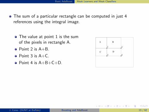
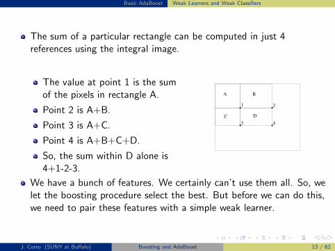
The sum of a particular rectangle can be computed in just 4references using the integral image.
The value at point 1 is the sumof the pixels in rectangle A.
Point 2 is A+B.
Point 3 is A+C.
Point 4 is A+B+C+D.
So, the sum within D alone is4+1-2-3.
A
C
B
D
1
4
2
3
Figure 2: The sum of the pixels within rectangle can be
computed with four array references. The value of the inte-
gral image at location 1 is the sum of the pixels in rectangle
. The value at location 2 is , at location 3 is ,
and at location 4 is . The sum within can
be computed as .
where is the integral image and is the origi-
nal image. Using the following pair of recurrences:
(1)
(2)
(where is the cumulative row sum, ,
and ) the integral image can be computed in
one pass over the original image.
Using the integral image any rectangular sum can be
computed in four array references (see Figure 2). Clearly
the difference between two rectangular sums can be com-
puted in eight references. Since the two-rectangle features
defined above involve adjacent rectangular sums they can
be computed in six array references, eight in the case of
the three-rectangle features, and nine for four-rectangle fea-
tures.
2.2. Feature Discussion
Rectangle features are somewhat primitive when compared
with alternatives such as steerable filters [5, 7]. Steerable fil-
ters, and their relatives, are excellent for the detailed analy-
sis of boundaries, image compression, and texture analysis.
In contrast rectangle features, while sensitive to the pres-
ence of edges, bars, and other simple image structure, are
quite coarse. Unlike steerable filters the only orientations
available are vertical, horizontal, and diagonal. The set of
rectangle features do however provide a rich image repre-
sentation which supports effective learning. In conjunction
with the integral image , the efficiency of the rectangle fea-
ture set provides ample compensation for their limited flex-
ibility.
3. Learning Classification Functions
Given a feature set and a training set of positive and neg-
ative images, any number of machine learning approaches
could be used to learn a classification function. In our sys-
tem a variant of AdaBoost is used both to select a small set
of features and train the classifier [6]. In its original form,
the AdaBoost learning algorithm is used to boost the clas-
sification performance of a simple (sometimes called weak)
learning algorithm. There are a number of formal guaran-
tees provided by the AdaBoost learning procedure. Freund
and Schapire proved that the training error of the strong
classifier approaches zero exponentially in the number of
rounds. More importantly a number of results were later
proved about generalization performance [14]. The key
insight is that generalization performance is related to the
margin of the examples, and that AdaBoost achieves large
margins rapidly.
Recall that there are over 180,000 rectangle features as-
sociated with each image sub-window, a number far larger
than the number of pixels. Even though each feature can
be computed very efficiently, computing the complete set is
prohibitively expensive. Our hypothesis, which is borne out
by experiment, is that a very small number of these features
can be combined to form an effective classifier. The main
challenge is to find these features.
In support of this goal, the weak learning algorithm is
designed to select the single rectangle feature which best
separates the positive and negative examples (this is similar
to the approach of [2] in the domain of image database re-
trieval). For each feature, the weak learner determines the
optimal threshold classification function, such that the min-
imum number of examples are misclassified. A weak clas-
sifier thus consists of a feature , a threshold and
a parity indicating the direction of the inequality sign:
if
otherwise
Here is a 24x24 pixel sub-window of an image. See Ta-
ble 1 for a summary of the boosting process.
In practice no single feature can perform the classifica-
tion task with low error. Features which are selected in early
rounds of the boosting process had error rates between 0.1
and 0.3. Features selected in later rounds, as the task be-
comes more difficult, yield error rates between 0.4 and 0.5.
3.1. Learning Discussion
Many general feature selection procedures have been pro-
posed (see chapter 8 of [18] for a review). Our final appli-
cation demanded a very aggressive approach which would
discard the vast majority of features. For a similar recogni-
tion problem Papageorgiou et al. proposed a scheme for fea-
ture selection based on feature variance [10]. They demon-
strated good results selecting 37 features out of a total 1734
features.
Roth et al. propose a feature selection process based
on the Winnow exponential perceptron learning rule [11].
TheWinnow learning process converges to a solution where
many of these weights are zero. Nevertheless a very large
3
We have a bunch of features. We certainly can’t use them all. So, welet the boosting procedure select the best. But before we can do this,we need to pair these features with a simple weak learner.
J. Corso (SUNY at Buffalo) Boosting and AdaBoost 13 / 62

Basic AdaBoost Weak Learners and Weak Classifiers
The sum of a particular rectangle can be computed in just 4references using the integral image.
The value at point 1 is the sumof the pixels in rectangle A.
Point 2 is A+B.
Point 3 is A+C.
Point 4 is A+B+C+D.
So, the sum within D alone is4+1-2-3.
A
C
B
D
1
4
2
3
Figure 2: The sum of the pixels within rectangle can be
computed with four array references. The value of the inte-
gral image at location 1 is the sum of the pixels in rectangle
. The value at location 2 is , at location 3 is ,
and at location 4 is . The sum within can
be computed as .
where is the integral image and is the origi-
nal image. Using the following pair of recurrences:
(1)
(2)
(where is the cumulative row sum, ,
and ) the integral image can be computed in
one pass over the original image.
Using the integral image any rectangular sum can be
computed in four array references (see Figure 2). Clearly
the difference between two rectangular sums can be com-
puted in eight references. Since the two-rectangle features
defined above involve adjacent rectangular sums they can
be computed in six array references, eight in the case of
the three-rectangle features, and nine for four-rectangle fea-
tures.
2.2. Feature Discussion
Rectangle features are somewhat primitive when compared
with alternatives such as steerable filters [5, 7]. Steerable fil-
ters, and their relatives, are excellent for the detailed analy-
sis of boundaries, image compression, and texture analysis.
In contrast rectangle features, while sensitive to the pres-
ence of edges, bars, and other simple image structure, are
quite coarse. Unlike steerable filters the only orientations
available are vertical, horizontal, and diagonal. The set of
rectangle features do however provide a rich image repre-
sentation which supports effective learning. In conjunction
with the integral image , the efficiency of the rectangle fea-
ture set provides ample compensation for their limited flex-
ibility.
3. Learning Classification Functions
Given a feature set and a training set of positive and neg-
ative images, any number of machine learning approaches
could be used to learn a classification function. In our sys-
tem a variant of AdaBoost is used both to select a small set
of features and train the classifier [6]. In its original form,
the AdaBoost learning algorithm is used to boost the clas-
sification performance of a simple (sometimes called weak)
learning algorithm. There are a number of formal guaran-
tees provided by the AdaBoost learning procedure. Freund
and Schapire proved that the training error of the strong
classifier approaches zero exponentially in the number of
rounds. More importantly a number of results were later
proved about generalization performance [14]. The key
insight is that generalization performance is related to the
margin of the examples, and that AdaBoost achieves large
margins rapidly.
Recall that there are over 180,000 rectangle features as-
sociated with each image sub-window, a number far larger
than the number of pixels. Even though each feature can
be computed very efficiently, computing the complete set is
prohibitively expensive. Our hypothesis, which is borne out
by experiment, is that a very small number of these features
can be combined to form an effective classifier. The main
challenge is to find these features.
In support of this goal, the weak learning algorithm is
designed to select the single rectangle feature which best
separates the positive and negative examples (this is similar
to the approach of [2] in the domain of image database re-
trieval). For each feature, the weak learner determines the
optimal threshold classification function, such that the min-
imum number of examples are misclassified. A weak clas-
sifier thus consists of a feature , a threshold and
a parity indicating the direction of the inequality sign:
if
otherwise
Here is a 24x24 pixel sub-window of an image. See Ta-
ble 1 for a summary of the boosting process.
In practice no single feature can perform the classifica-
tion task with low error. Features which are selected in early
rounds of the boosting process had error rates between 0.1
and 0.3. Features selected in later rounds, as the task be-
comes more difficult, yield error rates between 0.4 and 0.5.
3.1. Learning Discussion
Many general feature selection procedures have been pro-
posed (see chapter 8 of [18] for a review). Our final appli-
cation demanded a very aggressive approach which would
discard the vast majority of features. For a similar recogni-
tion problem Papageorgiou et al. proposed a scheme for fea-
ture selection based on feature variance [10]. They demon-
strated good results selecting 37 features out of a total 1734
features.
Roth et al. propose a feature selection process based
on the Winnow exponential perceptron learning rule [11].
TheWinnow learning process converges to a solution where
many of these weights are zero. Nevertheless a very large
3
We have a bunch of features. We certainly can’t use them all. So, welet the boosting procedure select the best. But before we can do this,we need to pair these features with a simple weak learner.
J. Corso (SUNY at Buffalo) Boosting and AdaBoost 13 / 62

Basic AdaBoost Weak Learners and Weak Classifiers
Each run, the weak learner is designed to select the single rectanglefeature which best separates the positive and negative examples.
The weak learner searches for the optimal threshold classificationfunction, such that the minimum number of examples aremisclassified.
The weak classifier ht(x) hence consists of the feature ft(x), athreshold θt, and a parity pt indicating the direction of the inequalitysign:
ht(x) =
{+1 if ptft(x) < ptθt
−1 otherwise.(7)
J. Corso (SUNY at Buffalo) Boosting and AdaBoost 14 / 62

Basic AdaBoost The AdaBoost Classifier
The Strong AdaBoost Classifier
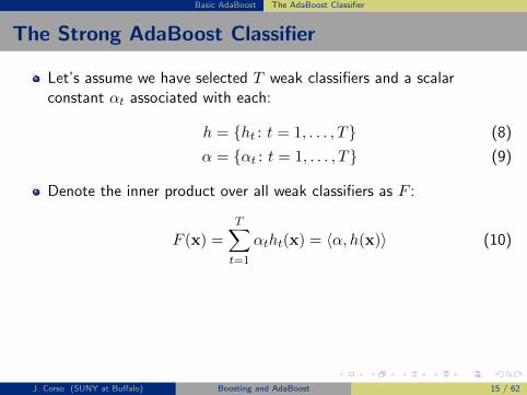
Let’s assume we have selected T weak classifiers and a scalarconstant αt associated with each:
h = {ht : t = 1, . . . , T} (8)
α = {αt : t = 1, . . . , T} (9)
Denote the inner product over all weak classifiers as F :
F (x) =T∑t=1
αtht(x) = 〈α, h(x)〉 (10)
Define the strong classifier as the sign of this inner product:
H(x) = sign [F (x)] = sign
[T∑t=1
αtht(x)
](11)
J. Corso (SUNY at Buffalo) Boosting and AdaBoost 15 / 62
Basic AdaBoost The AdaBoost Classifier
The Strong AdaBoost Classifier
Let’s assume we have selected T weak classifiers and a scalarconstant αt associated with each:
h = {ht : t = 1, . . . , T} (8)
α = {αt : t = 1, . . . , T} (9)
Denote the inner product over all weak classifiers as F :
F (x) =
T∑t=1
αtht(x) = 〈α, h(x)〉 (10)
Define the strong classifier as the sign of this inner product:
H(x) = sign [F (x)] = sign
[T∑t=1
αtht(x)
](11)
J. Corso (SUNY at Buffalo) Boosting and AdaBoost 15 / 62
Basic AdaBoost The AdaBoost Classifier
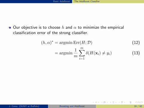
Our objective is to choose h and α to minimize the empiricalclassification error of the strong classifier.
(h, α)∗ = argminErr(H;D) (12)
= argmin1
m
m∑i=1
δ(H(xi) 6= yi) (13)
Adaboost doesn’t directly minimize this error but rather minimizes anupper bound on it.
J. Corso (SUNY at Buffalo) Boosting and AdaBoost 16 / 62

Basic AdaBoost The AdaBoost Classifier
Illustration of AdaBoost Classifier
Weak Learner
Input
J. Corso (SUNY at Buffalo) Boosting and AdaBoost 17 / 62

Basic AdaBoost The AdaBoost Algorithm
The Basic AdaBoost Algorithm
Given D = (xi, yi), . . . , (xm, ym) as before.Initialize the distribution D1 to be uniform: D1(i) =
1m .
Repeat for t = 1, . . . , T :
1 Learn weak classifier ht using distribution Dt.
For the example given, this requires you to learn the threshold and theparity at each iteration given the current distribution Dt for the weakclassifier h over each feature:
1 Compute the weighted error for each weak classifier.
εt(h) =m∑i=1
Dt(i)δ(h(xi) 6= yi), ∀h (14)
2 Select the weak classifier with minimum error.
ht = argminh εt(h) (15)
Note, there are other ways of doing this step...
J. Corso (SUNY at Buffalo) Boosting and AdaBoost 18 / 62

Basic AdaBoost The AdaBoost Algorithm
The Basic AdaBoost Algorithm
Given D = (xi, yi), . . . , (xm, ym) as before.Initialize the distribution D1 to be uniform: D1(i) =
1m .
Repeat for t = 1, . . . , T :
1 Learn weak classifier ht using distribution Dt.
For the example given, this requires you to learn the threshold and theparity at each iteration given the current distribution Dt for the weakclassifier h over each feature:
1 Compute the weighted error for each weak classifier.
εt(h) =
m∑i=1
Dt(i)δ(h(xi) 6= yi), ∀h (14)
2 Select the weak classifier with minimum error.
ht = argminh εt(h) (15)
Note, there are other ways of doing this step...
J. Corso (SUNY at Buffalo) Boosting and AdaBoost 18 / 62
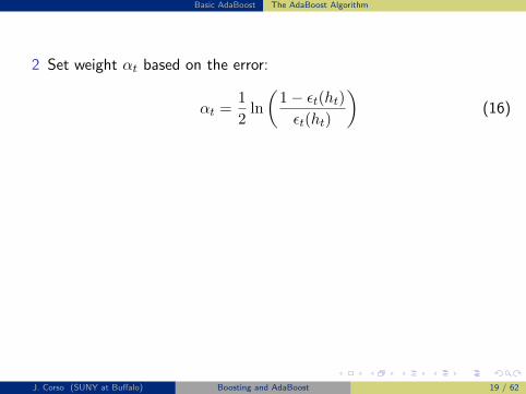
Basic AdaBoost The AdaBoost Algorithm
2 Set weight αt based on the error:
αt =1
2ln
(1− εt(ht)εt(ht)
)(16)
3 Update the distribution based on the performance so far:
Dt+1(i) =1
ZtDt(i) exp [−αtyiht(xi)] (17)
where Zt is a normalization factor to keep Dt+1 a distribution. Notethe careful evaluation of the term inside of the exp based on thepossible {−1,+1} values of the label.
One chooses T based on some established error criterion or somefixed number.
J. Corso (SUNY at Buffalo) Boosting and AdaBoost 19 / 62

AdaBoost Analysis
Contents for AdaBoost Analysis
Facts about the weights and normalizing functions.
AdaBoost Convergence (why and how fast).
Why do we calculate the weight of each weak classifier to be
αt =1
2ln
1− εt(ht)εt(ht)
?
Why do we choose the weak classifier that has the minimum weightederror?
Testing Error Analysis.
J. Corso (SUNY at Buffalo) Boosting and AdaBoost 20 / 62
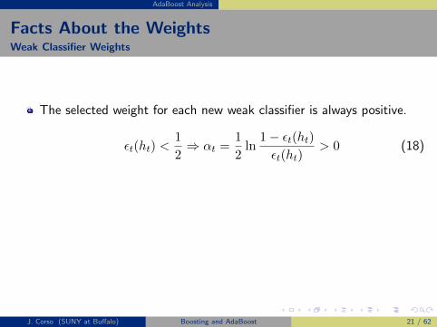
AdaBoost Analysis
Facts About the WeightsWeak Classifier Weights
The selected weight for each new weak classifier is always positive.
εt(ht) <1
2⇒ αt =
1
2ln
1− εt(ht)εt(ht)
> 0 (18)
The smaller the classification error, the bigger the weight and themore this particular weak classifier will impact the final strongclassifier.
ε(hA) < ε(hB)⇒ αA > αB (19)
J. Corso (SUNY at Buffalo) Boosting and AdaBoost 21 / 62
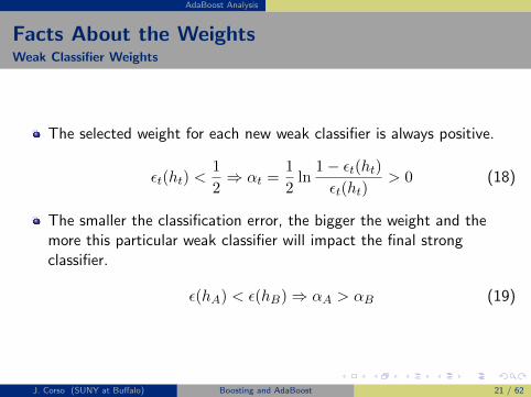

AdaBoost Analysis
Facts About the WeightsData Sample Weights
The weights of the data points are multiplied by exp [−yiαtht(xi)].
exp [−yiαtht(xi)] =
{exp [−αt] < 1 if ht(xi) = yi
exp [αt] > 1 if ht(xi) 6= yi(20)
The weights of correctly classified points are reduced and the weightsof incorrectly classified points are increased. Hence, the incorrectlyclassified points will receive more attention in the next run.
J. Corso (SUNY at Buffalo) Boosting and AdaBoost 22 / 62
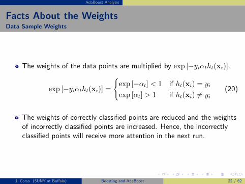

AdaBoost Analysis
The weight distribution can be computed recursively:
Dt+1(i) =1
ZtDt(i) exp [−αtyiht(xi)] (21)
=1
Zt−1ZtDt−1(i) exp
[−yi(αtht(xi) + αt−1ht−1(xi)
)]= . . .
=1
Z1 . . . ZtD1(i) exp
[−yi(αtht(xi) + · · ·+ α1h1(xi)
)]
J. Corso (SUNY at Buffalo) Boosting and AdaBoost 23 / 62

AdaBoost Analysis
Facts About the Normalizing Functions
At each iteration, the weights on the data points are normalized by
Zt =∑xi
Dt(xi) exp [−yiαiht(xi)] (22)
=∑xi∈A
Dt(xi) exp [−αt] +∑xi∈A
Dt(xi) exp [αt] (23)
where A is the set of correctly classified points: {xi : yi = ht(xi)}.
We can write these normalization factors as functions of αt, then:
Zt = Zt(αt) (24)
J. Corso (SUNY at Buffalo) Boosting and AdaBoost 24 / 62
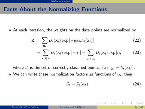
AdaBoost Analysis
Facts About the Normalizing Functions
At each iteration, the weights on the data points are normalized by
Zt =∑xi
Dt(xi) exp [−yiαiht(xi)] (22)
=∑xi∈A
Dt(xi) exp [−αt] +∑xi∈A
Dt(xi) exp [αt] (23)
where A is the set of correctly classified points: {xi : yi = ht(xi)}.We can write these normalization factors as functions of αt, then:
Zt = Zt(αt) (24)
J. Corso (SUNY at Buffalo) Boosting and AdaBoost 24 / 62
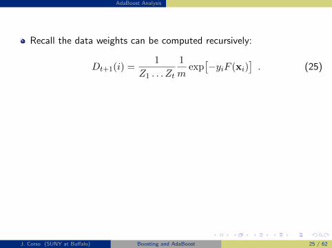
AdaBoost Analysis
Recall the data weights can be computed recursively:
Dt+1(i) =1
Z1 . . . Zt
1
mexp[−yiF (xi)
]. (25)
And, since we know the data weights must sum to one, we have
m∑i=1
Dt(xi) =1
Z1 . . . Zt
1
m
m∑i=1
exp[−yiF (xi)
]= 1 (26)
Therefore, we can summarize this with a new normalizing function:
Z = Z1 . . . Zt =1
m
m∑i=1
exp[−yiF (xi)
]. (27)
J. Corso (SUNY at Buffalo) Boosting and AdaBoost 25 / 62
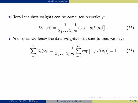
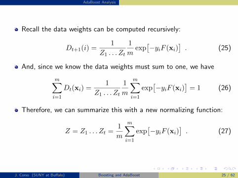

AdaBoost Analysis AdaBoost Convergence
AdaBoost Convergence
Key Idea: AdaBoost minimizes an upper bound on theclassification error.
Claim: After t steps, the error of the strong classifier is boundedabove by quantity Z, as we just defined it (the product of the dataweight normalization factors):
Err(H) ≤ Z = Z(α, h) = Zt(αt, ht) . . . Z1(α1, h1) (28)
AdaBoost is a greedy algorithm that minimizes this upper bound onthe classification error by choosing the optimal ht and αt to minimizeZt at each step.
(h, α)∗ = argminZ(α, h) (29)
(ht, αt)∗ = argminZt(αt, ht) (30)
As Z goes to zero, the classification error goes to zero. Hence, itconverges. (But, we need to account for the case when no new weak
classifier has an error rate better than 0.5, upon which time we should stop.)
J. Corso (SUNY at Buffalo) Boosting and AdaBoost 26 / 62

AdaBoost Analysis AdaBoost Convergence
AdaBoost Convergence
Key Idea: AdaBoost minimizes an upper bound on theclassification error.Claim: After t steps, the error of the strong classifier is boundedabove by quantity Z, as we just defined it (the product of the dataweight normalization factors):
Err(H) ≤ Z = Z(α, h) = Zt(αt, ht) . . . Z1(α1, h1) (28)
AdaBoost is a greedy algorithm that minimizes this upper bound onthe classification error by choosing the optimal ht and αt to minimizeZt at each step.
(h, α)∗ = argminZ(α, h) (29)
(ht, αt)∗ = argminZt(αt, ht) (30)
As Z goes to zero, the classification error goes to zero. Hence, itconverges. (But, we need to account for the case when no new weak
classifier has an error rate better than 0.5, upon which time we should stop.)
J. Corso (SUNY at Buffalo) Boosting and AdaBoost 26 / 62
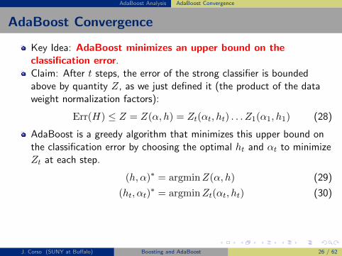
AdaBoost Analysis AdaBoost Convergence
AdaBoost Convergence
Key Idea: AdaBoost minimizes an upper bound on theclassification error.Claim: After t steps, the error of the strong classifier is boundedabove by quantity Z, as we just defined it (the product of the dataweight normalization factors):
Err(H) ≤ Z = Z(α, h) = Zt(αt, ht) . . . Z1(α1, h1) (28)
AdaBoost is a greedy algorithm that minimizes this upper bound onthe classification error by choosing the optimal ht and αt to minimizeZt at each step.
(h, α)∗ = argminZ(α, h) (29)
(ht, αt)∗ = argminZt(αt, ht) (30)
As Z goes to zero, the classification error goes to zero. Hence, itconverges. (But, we need to account for the case when no new weak
classifier has an error rate better than 0.5, upon which time we should stop.)
J. Corso (SUNY at Buffalo) Boosting and AdaBoost 26 / 62
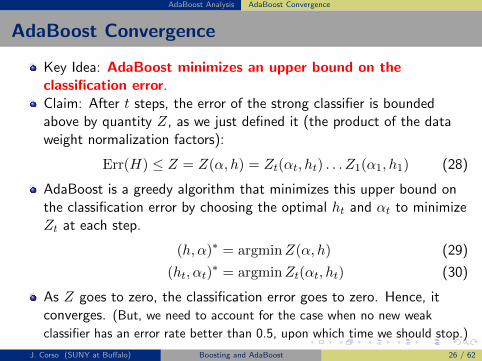
AdaBoost Analysis AdaBoost Convergence
AdaBoost Convergence
Key Idea: AdaBoost minimizes an upper bound on theclassification error.Claim: After t steps, the error of the strong classifier is boundedabove by quantity Z, as we just defined it (the product of the dataweight normalization factors):
Err(H) ≤ Z = Z(α, h) = Zt(αt, ht) . . . Z1(α1, h1) (28)
AdaBoost is a greedy algorithm that minimizes this upper bound onthe classification error by choosing the optimal ht and αt to minimizeZt at each step.
(h, α)∗ = argminZ(α, h) (29)
(ht, αt)∗ = argminZt(αt, ht) (30)
As Z goes to zero, the classification error goes to zero. Hence, itconverges. (But, we need to account for the case when no new weak
classifier has an error rate better than 0.5, upon which time we should stop.)
J. Corso (SUNY at Buffalo) Boosting and AdaBoost 26 / 62

AdaBoost Analysis AdaBoost Convergence
We need to show the claim on the error bound is true:
Err(H) =1
m
m∑i=1
δ(H(xi) 6= yi) ≤ Z =1
m
m∑i=1
exp [−yiF (xi)] (31)
Proof:
F (xi) = sign(F (xi))|F (xi)| (32)
= H(xi)|F (xi)| (33)
The two cases are:
If H(xi) 6= yi then the LHS = 1 ≤ RHS = e+|F (xi)|.If H(xi) = yi then the LHS = 0 ≤ RHS = e−|F (xi)|.
So, the inequality holds for each term
δ(H(xi) 6= yi) ≤ exp [−yiF (xi)] (34)
and hence, the inequality is true.
J. Corso (SUNY at Buffalo) Boosting and AdaBoost 27 / 62
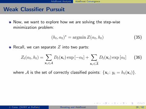
AdaBoost Analysis AdaBoost Convergence
Weak Classifier Pursuit
Now, we want to explore how we are solving the step-wiseminimization problem:
(ht, αt)∗ = argminZ(αt, ht) (35)
Recall, we can separate Z into two parts:
Zt(αt, ht) =∑xi∈A
Dt(xi) exp [−αt] +∑xi∈A
Dt(xi) exp [αt] (36)
where A is the set of correctly classified points: {xi : yi = ht(xi)}.
Take the derivative w.r.t. αt and set it to zero:
dZt(αt, ht)
dαt=∑xi∈A
−Dt(xi) exp [−αt] +∑xi∈A
Dt(xi) exp [αt] = 0 (37)
J. Corso (SUNY at Buffalo) Boosting and AdaBoost 28 / 62

AdaBoost Analysis AdaBoost Convergence
Weak Classifier Pursuit
Now, we want to explore how we are solving the step-wiseminimization problem:
(ht, αt)∗ = argminZ(αt, ht) (35)
Recall, we can separate Z into two parts:
Zt(αt, ht) =∑xi∈A
Dt(xi) exp [−αt] +∑xi∈A
Dt(xi) exp [αt] (36)
where A is the set of correctly classified points: {xi : yi = ht(xi)}.Take the derivative w.r.t. αt and set it to zero:
dZt(αt, ht)
dαt=∑xi∈A
−Dt(xi) exp [−αt] +∑xi∈A
Dt(xi) exp [αt] = 0 (37)
J. Corso (SUNY at Buffalo) Boosting and AdaBoost 28 / 62
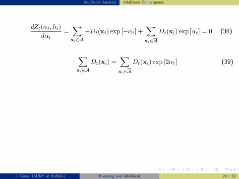
AdaBoost Analysis AdaBoost Convergence
dZt(αt, ht)
dαt=∑xi∈A
−Dt(xi) exp [−αt] +∑xi∈A
Dt(xi) exp [αt] = 0 (38)
∑xi∈A
Dt(xi) =∑xi∈A
Dt(xi) exp [2αt] (39)
And, by definition, we can write the error as
εt(h) =
m∑i=1
Dt(xi)δ(h(xi) 6= yi) =∑xi∈A
Dt(xi), ∀h (40)
Rewriting (39) and solving for αt yields
αt =1
2ln
1− εt(ht)εt(ht)
(41)
J. Corso (SUNY at Buffalo) Boosting and AdaBoost 29 / 62
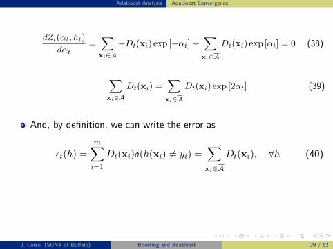

AdaBoost Analysis AdaBoost Convergence
We can plug it back into the normalization term to get the minimum:
Zt(αt, ht) =∑xi∈A
Dt(xi) exp [−αt] +∑xi∈A
Dt(xi) exp [αt] (42)
= (1− εt(ht))
√εt(ht)
1− εt(ht)+ εt(ht)
√1− εt(ht)εt(ht)
(43)
= 2√εt(ht)(1− εt(ht)) (44)
Change a variable, γt =12 − εt(ht), γt ∈ (0, 12 ].
Then, we have the minimum to be
Zt(αt, ht) = 2√εt(ht)(1− εt(ht)) (45)
=√1− 4γ2t (46)
≤ exp[−2γ2t
](47)
J. Corso (SUNY at Buffalo) Boosting and AdaBoost 30 / 62

AdaBoost Analysis AdaBoost Convergence
We can plug it back into the normalization term to get the minimum:
Zt(αt, ht) =∑xi∈A
Dt(xi) exp [−αt] +∑xi∈A
Dt(xi) exp [αt] (42)
= (1− εt(ht))
√εt(ht)
1− εt(ht)+ εt(ht)
√1− εt(ht)εt(ht)
(43)
= 2√εt(ht)(1− εt(ht)) (44)
Change a variable, γt =12 − εt(ht), γt ∈ (0, 12 ].
Then, we have the minimum to be
Zt(αt, ht) = 2√εt(ht)(1− εt(ht)) (45)
=√
1− 4γ2t (46)
≤ exp[−2γ2t
](47)
J. Corso (SUNY at Buffalo) Boosting and AdaBoost 30 / 62
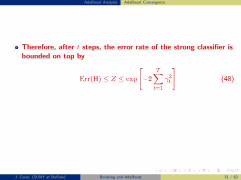
AdaBoost Analysis AdaBoost Convergence
Therefore, after t steps, the error rate of the strong classifier isbounded on top by
Err(H) ≤ Z ≤ exp
[−2
T∑t=1
γ2t
](48)
Hence, each step decreases the upper bound exponentially.
And, a weak classifier with small error rate will lead to faster descent.
J. Corso (SUNY at Buffalo) Boosting and AdaBoost 31 / 62
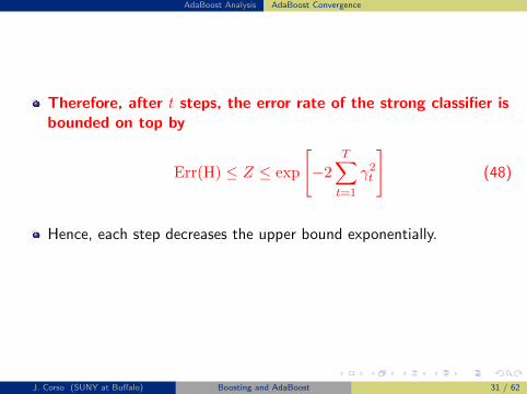
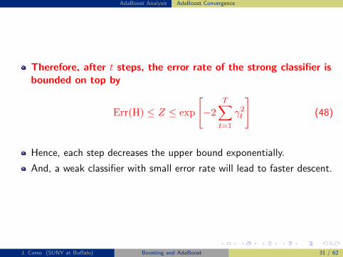

AdaBoost Analysis AdaBoost Convergence
Summary of AdaBoost Convergence
The objective of AdaBoost is to minimize an upper bound on theclassification error:
(α, h)∗ = argminZ(α, h) (49)
= argminZt(αt, ht) . . . Z1(α1, h1) (50)
= argminm∑i=1
exp [−yi〈α, h(xi)〉] (51)
AdaBoost takes a stepwise minimization scheme, which may not beoptimal (it is greedy). When we calculate the parameter for the tth
weak classifier, the others remain set.
We should stop AdaBoost if all of the weak classifiers have an errorrate of 1
2 .
J. Corso (SUNY at Buffalo) Boosting and AdaBoost 32 / 62
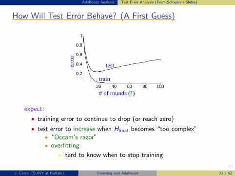
AdaBoost Analysis Test Error Analysis (From Schapire’s Slides)
How Will Test Error Behave? (A First Guess)How Will Test Error Behave? (A First Guess)How Will Test Error Behave? (A First Guess)How Will Test Error Behave? (A First Guess)How Will Test Error Behave? (A First Guess)
20 40 60 80 100
0.2
0.4
0.6
0.8
1
# of rounds (
erro
r
T)
train
test
expect:
• training error to continue to drop (or reach zero)
• test error to increase when Hfinal becomes “too complex”• “Occam’s razor”• overfitting
• hard to know when to stop training
J. Corso (SUNY at Buffalo) Boosting and AdaBoost 33 / 62

AdaBoost Analysis Test Error Analysis (From Schapire’s Slides)
Actual Typical RunActual Typical RunActual Typical RunActual Typical RunActual Typical Run
10 100 10000
5
10
15
20
# of rounds (T
C4.5 test error
)
train
test
erro
r
(boosting C4.5 on“letter” dataset)
• test error does not increase, even after 1000 rounds• (total size > 2,000,000 nodes)
• test error continues to drop even after training error is zero!
# rounds5 100 1000
train error 0.0 0.0 0.0
test error 8.4 3.3 3.1
• Occam’s razor wrongly predicts “simpler” rule is better
J. Corso (SUNY at Buffalo) Boosting and AdaBoost 34 / 62

AdaBoost Analysis Test Error Analysis (From Schapire’s Slides)
A Better Story: The Margins ExplanationA Better Story: The Margins ExplanationA Better Story: The Margins ExplanationA Better Story: The Margins ExplanationA Better Story: The Margins Explanation[with Freund, Bartlett & Lee]
• key idea:• training error only measures whether classifications are
right or wrong• should also consider confidence of classifications
J. Corso (SUNY at Buffalo) Boosting and AdaBoost 35 / 62
AdaBoost Analysis Test Error Analysis (From Schapire’s Slides)
A Better Story: The Margins ExplanationA Better Story: The Margins ExplanationA Better Story: The Margins ExplanationA Better Story: The Margins ExplanationA Better Story: The Margins Explanation[with Freund, Bartlett & Lee]
• key idea:• training error only measures whether classifications are
right or wrong• should also consider confidence of classifications
• recall: Hfinal is weighted majority vote of weak classifiers
J. Corso (SUNY at Buffalo) Boosting and AdaBoost 36 / 62
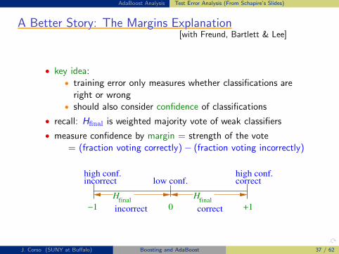
AdaBoost Analysis Test Error Analysis (From Schapire’s Slides)
A Better Story: The Margins ExplanationA Better Story: The Margins ExplanationA Better Story: The Margins ExplanationA Better Story: The Margins ExplanationA Better Story: The Margins Explanation[with Freund, Bartlett & Lee]
• key idea:• training error only measures whether classifications are
right or wrong• should also consider confidence of classifications
• recall: Hfinal is weighted majority vote of weak classifiers
• measure confidence by margin = strength of the vote= (fraction voting correctly)− (fraction voting incorrectly)
correctincorrect
correctincorrect
0
high conf. high conf.low conf.
−1 +1final
Hfinal
H
J. Corso (SUNY at Buffalo) Boosting and AdaBoost 37 / 62

AdaBoost Analysis Test Error Analysis (From Schapire’s Slides)
Empirical Evidence: The Margin DistributionEmpirical Evidence: The Margin DistributionEmpirical Evidence: The Margin DistributionEmpirical Evidence: The Margin DistributionEmpirical Evidence: The Margin Distribution
• margin distribution= cumulative distribution of margins of training examples
10 100 10000
5
10
15
20
erro
r
test
train
)T# of rounds (-1 -0.5 0.5 1
0.5
1.0
cum
ulat
ive
dist
ribu
tion
1000100
margin
5
# rounds5 100 1000
train error 0.0 0.0 0.0
test error 8.4 3.3 3.1
% margins ≤ 0.5 7.7 0.0 0.0
minimum margin 0.14 0.52 0.55
J. Corso (SUNY at Buffalo) Boosting and AdaBoost 38 / 62

AdaBoost Analysis Test Error Analysis (From Schapire’s Slides)
Theoretical Evidence: Analyzing Boosting Using MarginsTheoretical Evidence: Analyzing Boosting Using MarginsTheoretical Evidence: Analyzing Boosting Using MarginsTheoretical Evidence: Analyzing Boosting Using MarginsTheoretical Evidence: Analyzing Boosting Using Margins
• Theorem: large margins ⇒ better bound on generalizationerror (independent of number of rounds)
J. Corso (SUNY at Buffalo) Boosting and AdaBoost 39 / 62

AdaBoost Analysis Test Error Analysis (From Schapire’s Slides)
Theoretical Evidence: Analyzing Boosting Using MarginsTheoretical Evidence: Analyzing Boosting Using MarginsTheoretical Evidence: Analyzing Boosting Using MarginsTheoretical Evidence: Analyzing Boosting Using MarginsTheoretical Evidence: Analyzing Boosting Using Margins
• Theorem: large margins ⇒ better bound on generalizationerror (independent of number of rounds)
• proof idea: if all margins are large, then can approximatefinal classifier by a much smaller classifier (just as pollscan predict not-too-close election)
J. Corso (SUNY at Buffalo) Boosting and AdaBoost 40 / 62

AdaBoost Analysis Test Error Analysis (From Schapire’s Slides)
Theoretical Evidence: Analyzing Boosting Using MarginsTheoretical Evidence: Analyzing Boosting Using MarginsTheoretical Evidence: Analyzing Boosting Using MarginsTheoretical Evidence: Analyzing Boosting Using MarginsTheoretical Evidence: Analyzing Boosting Using Margins
• Theorem: large margins ⇒ better bound on generalizationerror (independent of number of rounds)
• proof idea: if all margins are large, then can approximatefinal classifier by a much smaller classifier (just as pollscan predict not-too-close election)
• Theorem: boosting tends to increase margins of trainingexamples (given weak learning assumption)
J. Corso (SUNY at Buffalo) Boosting and AdaBoost 41 / 62
AdaBoost Analysis Test Error Analysis (From Schapire’s Slides)
Theoretical Evidence: Analyzing Boosting Using MarginsTheoretical Evidence: Analyzing Boosting Using MarginsTheoretical Evidence: Analyzing Boosting Using MarginsTheoretical Evidence: Analyzing Boosting Using MarginsTheoretical Evidence: Analyzing Boosting Using Margins
• Theorem: large margins ⇒ better bound on generalizationerror (independent of number of rounds)
• proof idea: if all margins are large, then can approximatefinal classifier by a much smaller classifier (just as pollscan predict not-too-close election)
• Theorem: boosting tends to increase margins of trainingexamples (given weak learning assumption)
• proof idea: similar to training error proof
J. Corso (SUNY at Buffalo) Boosting and AdaBoost 42 / 62
AdaBoost Analysis Test Error Analysis (From Schapire’s Slides)
Theoretical Evidence: Analyzing Boosting Using MarginsTheoretical Evidence: Analyzing Boosting Using MarginsTheoretical Evidence: Analyzing Boosting Using MarginsTheoretical Evidence: Analyzing Boosting Using MarginsTheoretical Evidence: Analyzing Boosting Using Margins
• Theorem: large margins ⇒ better bound on generalizationerror (independent of number of rounds)
• proof idea: if all margins are large, then can approximatefinal classifier by a much smaller classifier (just as pollscan predict not-too-close election)
• Theorem: boosting tends to increase margins of trainingexamples (given weak learning assumption)
• proof idea: similar to training error proof
• so:although final classifier is getting larger,margins are likely to be increasing,so final classifier actually getting close to a simpler classifier,driving down the test error
J. Corso (SUNY at Buffalo) Boosting and AdaBoost 43 / 62

AdaBoost Analysis Test Error Analysis (From Schapire’s Slides)
More Technically...More Technically...More Technically...More Technically...More Technically...
• with high probability, ∀θ > 0 :
generalization error ≤ Pr[margin ≤ θ] + O
(
√
d/m
θ
)
(Pr[ ] = empirical probability)
• bound depends on
• m = # training examples• d = “complexity” of weak classifiers• entire distribution of margins of training examples
• Pr[margin ≤ θ]→ 0 exponentially fast (in T ) if(error of ht on Dt) < 1/2− θ (∀t)
• so: if weak learning assumption holds, then all exampleswill quickly have “large” margins
J. Corso (SUNY at Buffalo) Boosting and AdaBoost 44 / 62

AdaBoost Recap
Summary of Basic AdaBoost
AdaBoost is a sequential algorithm that minimizes an upper bound ofthe empirical classification error by selecting the weak classifiers andtheir weights. These are “pursued” one-by-one with each one beingselected to maximally reduce the upper bound of error.
AdaBoost defines a distribution of weights over the data samples.These weights are updated each time a new weak classifier is addedsuch that samples misclassified by this new weak classifiers are givenmore weight. In this manner, currently misclassified samples areemphasized more during the selection of the subsequent weakclassifier.
The empirical error will converge to zero at an exponential rate.
J. Corso (SUNY at Buffalo) Boosting and AdaBoost 45 / 62
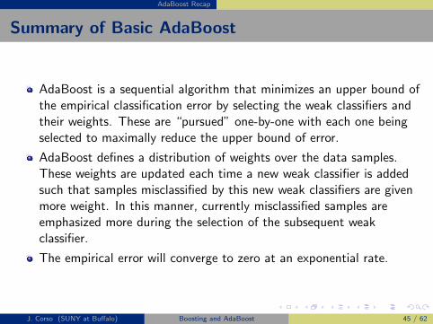

AdaBoost Recap
Practical AdaBoost Advantages
It is fast to evaluate (linear-additive) and can be fast to train(depending on weak learner).
T is the only parameter to tune.
It is flexible and can be combined with any weak learner.
It is provably effective if it can consistently find the weak classifiers(that do better than random).
Since it can work with any weak learner, it can handle the gamut ofdata.
J. Corso (SUNY at Buffalo) Boosting and AdaBoost 46 / 62

AdaBoost Recap
AdaBoost Caveats
Performance depends on the data and the weak learner.
It can fail if
The weak classifiers are too complex and overfit.
The weak classifiers are too weak, essentially underfitting.
AdaBoost seems, empirically, to be especially susceptible to uniformnoise.
J. Corso (SUNY at Buffalo) Boosting and AdaBoost 47 / 62
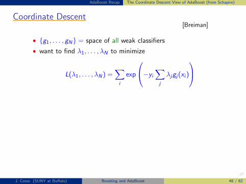
AdaBoost Recap The Coordinate Descent View of AdaBoost (from Schapire)
Coordinate DescentCoordinate DescentCoordinate DescentCoordinate DescentCoordinate Descent[Breiman]
• {g1, . . . , gN} = space of all weak classifiers
• want to find λ1, . . . , λN to minimize
L(λ1, . . . , λN) =∑
i
exp
−yi
∑
j
λjgj(xi )
J. Corso (SUNY at Buffalo) Boosting and AdaBoost 48 / 62

AdaBoost Recap The Coordinate Descent View of AdaBoost (from Schapire)
Coordinate DescentCoordinate DescentCoordinate DescentCoordinate DescentCoordinate Descent[Breiman]
• {g1, . . . , gN} = space of all weak classifiers
• want to find λ1, . . . , λN to minimize
L(λ1, . . . , λN) =∑
i
exp
−yi
∑
j
λjgj(xi )
• AdaBoost is actually doing coordinate descent on thisoptimization problem:
• initially, all λj = 0• each round: choose one coordinate λj (corresponding to
ht) and update (increment by αt)• choose update causing biggest decrease in loss
• powerful technique for minimizing over huge space offunctions
J. Corso (SUNY at Buffalo) Boosting and AdaBoost 49 / 62

AdaBoost for Estimating Conditional Probabilities
Estimating Conditional ProbabilitiesEstimating Conditional ProbabilitiesEstimating Conditional ProbabilitiesEstimating Conditional ProbabilitiesEstimating Conditional Probabilities[Friedman, Hastie & Tibshirani]
• often want to estimate probability that y = +1 given x
• AdaBoost minimizes (empirical version of):
Ex ,y
[
e−yf (x)]
= Ex
[
P [y = +1|x ] e−f (x) + P [y = −1|x ] ef (x)]
where x , y random from true distribution
J. Corso (SUNY at Buffalo) Boosting and AdaBoost 50 / 62
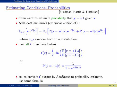
AdaBoost for Estimating Conditional Probabilities
Estimating Conditional ProbabilitiesEstimating Conditional ProbabilitiesEstimating Conditional ProbabilitiesEstimating Conditional ProbabilitiesEstimating Conditional Probabilities[Friedman, Hastie & Tibshirani]
• often want to estimate probability that y = +1 given x
• AdaBoost minimizes (empirical version of):
Ex ,y
[
e−yf (x)]
= Ex
[
P [y = +1|x ] e−f (x) + P [y = −1|x ] ef (x)]
where x , y random from true distribution
• over all f , minimized when
f (x) =1
2· ln
(
P [y = +1|x ]
P [y = −1|x ]
)
or
P [y = +1|x ] =1
1 + e−2f (x)
• so, to convert f output by AdaBoost to probability estimate,use same formula
J. Corso (SUNY at Buffalo) Boosting and AdaBoost 51 / 62

Multiclass AdaBoost From Schapire’s Slides
Multiclass ProblemsMulticlass ProblemsMulticlass ProblemsMulticlass ProblemsMulticlass Problems[with Freund]
• say y ∈ Y = {1, . . . , k}• direct approach (AdaBoost.M1):
ht : X → Y
Dt+1(i) =Dt(i)
Zt
·
{
e−αt if yi = ht(xi )eαt if yi 6= ht(xi )
Hfinal(x) = arg maxy∈Y
∑
t:ht(x)=y
αt
J. Corso (SUNY at Buffalo) Boosting and AdaBoost 52 / 62
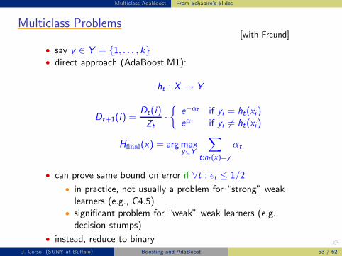
Multiclass AdaBoost From Schapire’s Slides
Multiclass ProblemsMulticlass ProblemsMulticlass ProblemsMulticlass ProblemsMulticlass Problems[with Freund]
• say y ∈ Y = {1, . . . , k}• direct approach (AdaBoost.M1):
ht : X → Y
Dt+1(i) =Dt(i)
Zt
·
{
e−αt if yi = ht(xi )eαt if yi 6= ht(xi )
Hfinal(x) = arg maxy∈Y
∑
t:ht(x)=y
αt
• can prove same bound on error if ∀t : εt ≤ 1/2
• in practice, not usually a problem for “strong” weaklearners (e.g., C4.5)
• significant problem for “weak” weak learners (e.g.,decision stumps)
• instead, reduce to binaryJ. Corso (SUNY at Buffalo) Boosting and AdaBoost 53 / 62
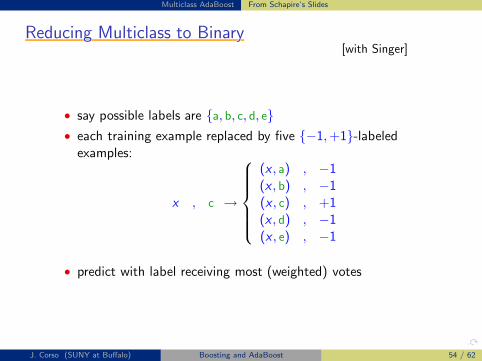
Multiclass AdaBoost From Schapire’s Slides
Reducing Multiclass to BinaryReducing Multiclass to BinaryReducing Multiclass to BinaryReducing Multiclass to BinaryReducing Multiclass to Binary[with Singer]
• say possible labels are {a, b, c, d, e}
• each training example replaced by five {−1,+1}-labeledexamples:
x , c →
(x , a) , −1(x , b) , −1(x , c) , +1(x , d) , −1(x , e) , −1
• predict with label receiving most (weighted) votes
J. Corso (SUNY at Buffalo) Boosting and AdaBoost 54 / 62

Applications
AdaBoost for Face Detection
Viola and Jones 2000-2002.Given example images where
for negative and positive examples respec-
tively.
Initialize weights for respec-
tively, where and are the number of negatives and
positives respectively.
For :
1. Normalize the weights,
so that is a probability distribution.
2. For each feature, , train a classifi er which
is restricted to using a single feature. The
error is evaluated with respect to ,
.
3. Choose the classifi er, , with the lowest error .
4. Update the weights:
where if example is classifi ed cor-
rectly, otherwise, and .
The fi nal strong classifi er is:
otherwise
where
Table 1: The AdaBoost algorithm for classifier learn-
ing. Each round of boosting selects one feature from the
180,000 potential features.
number of features are retained (perhaps a few hundred or
thousand).
3.2. Learning Results
While details on the training and performance of the final
system are presented in Section 5, several simple results
merit discussion. Initial experiments demonstrated that a
frontal face classifier constructed from 200 features yields
a detection rate of 95% with a false positive rate of 1 in
14084. These results are compelling, but not sufficient for
many real-world tasks. In terms of computation, this clas-
sifier is probably faster than any other published system,
requiring 0.7 seconds to scan an 384 by 288 pixel image.
Unfortunately, the most straightforward technique for im-
proving detection performance, adding features to the clas-
sifier, directly increases computation time.
For the task of face detection, the initial rectangle fea-
tures selected by AdaBoost are meaningful and easily inter-
preted. The first feature selected seems to focus on the prop-
erty that the region of the eyes is often darker than the region
Figure 3: The first and second features selected by Ad-
aBoost. The two features are shown in the top row and then
overlayed on a typical training face in the bottom row. The
first feature measures the difference in intensity between the
region of the eyes and a region across the upper cheeks. The
feature capitalizes on the observation that the eye region is
often darker than the cheeks. The second feature compares
the intensities in the eye regions to the intensity across the
bridge of the nose.
of the nose and cheeks (see Figure 3). This feature is rel-
atively large in comparison with the detection sub-window,
and should be somewhat insensitive to size and location of
the face. The second feature selected relies on the property
that the eyes are darker than the bridge of the nose.
4. The Attentional Cascade
This section describes an algorithm for constructing a cas-
cade of classifiers which achieves increased detection per-
formance while radically reducing computation time. The
key insight is that smaller, and therefore more efficient,
boosted classifiers can be constructed which reject many of
the negative sub-windows while detecting almost all posi-
tive instances (i.e. the threshold of a boosted classifier can
be adjusted so that the false negative rate is close to zero).
Simpler classifiers are used to reject the majority of sub-
windows before more complex classifiers are called upon
to achieve low false positive rates.
The overall form of the detection process is that of a de-
generate decision tree, what we call a “cascade” (see Fig-
ure 4). A positive result from the first classifier triggers the
evaluation of a second classifier which has also been ad-
justed to achieve very high detection rates. A positive result
from the second classifier triggers a third classifier, and so
on. A negative outcome at any point leads to the immediate
rejection of the sub-window.
Stages in the cascade are constructed by training clas-
sifiers using AdaBoost and then adjusting the threshold to
minimize false negatives. Note that the default AdaBoost
threshold is designed to yield a low error rate on the train-
ing data. In general a lower threshold yields higher detec-
4
J. Corso (SUNY at Buffalo) Boosting and AdaBoost 55 / 62
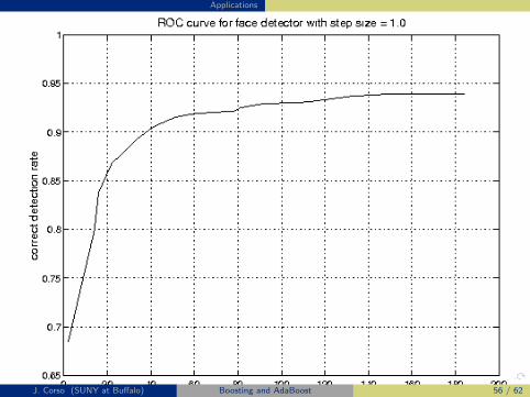
Applications
Figure 7: Output of our face detector on a number of test images from the MIT+CMU test set.
Figure 6: ROC curve for our face detector on the
MIT+CMU test set. The detector was run using a step size
of 1.0 and starting scale of 1.0 (75,081,800 sub-windows
scanned).
have broader application in computer vision and image pro-
cessing.
Finally this paper presents a set of detailed experiments
on a difficult face detection dataset which has been widely
studied. This dataset includes faces under a very wide range
of conditions including: illumination, scale, pose, and cam-
era variation. Experiments on such a large and complex
dataset are difficult and time consuming. Nevertheless sys-
tems which work under these conditions are unlikely to be
brittle or limited to a single set of conditions. More impor-
tantly conclusions drawn from this dataset are unlikely to
be experimental artifacts.
References
[1] Y. Amit, D. Geman, and K. Wilder. Joint induction of shape
features and tree classifi ers, 1997.
[2] Anonymous. Anonymous. In Anonymous, 2000.
[3] F. Crow. Summed-area tables for texture mapping. In
Proceedings of SIGGRAPH, volume 18(3), pages 207–212,
1984.
[4] F. Fleuret and D. Geman. Coarse-to-fi ne face detection. Int.
J. Computer Vision, 2001.
[5] William T. Freeman and Edward H. Adelson. The design
and use of steerable fi lters. IEEE Transactions on Pattern
Analysis and Machine Intelligence, 13(9):891–906, 1991.
[6] Yoav Freund and Robert E. Schapire. A decision-theoretic
generalization of on-line learning and an application to
boosting. In Computational Learning Theory: Eurocolt ’95,
pages 23–37. Springer-Verlag, 1995.
[7] H. Greenspan, S. Belongie, R. Gooodman, P. Perona, S. Rak-
shit, and C. Anderson. Overcomplete steerable pyramid fi l-
ters and rotation invariance. In Proceedings of the IEEECon-
ference on Computer Vision and Pattern Recognition, 1994.
[8] L. Itti, C. Koch, and E. Niebur. A model of saliency-based
visual attention for rapid scene analysis. IEEE Patt. Anal.
Mach. Intell., 20(11):1254–1259, November 1998.
[9] Edgar Osuna, Robert Freund, and Federico Girosi. Training
support vector machines: an application to face detection.
In Proceedings of the IEEE Conference on Computer Vision
and Pattern Recognition, 1997.
[10] C. Papageorgiou, M. Oren, and T. Poggio. A general frame-
work for object detection. In International Conference on
Computer Vision, 1998.
[11] D. Roth, M. Yang, and N. Ahuja. A snowbased face detector.
In Neural Information Processing 12, 2000.
[12] H. Rowley, S. Baluja, and T. Kanade. Neural network-based
face detection. In IEEE Patt. Anal. Mach. Intell., volume 20,
pages 22–38, 1998.
[13] R. E. Schapire, Y. Freund, P. Bartlett, and W. S. Lee. Boost-
ing the margin: a new explanation for the effectiveness of
voting methods. Ann. Stat., 26(5):1651–1686, 1998.
[14] Robert E. Schapire, Yoav Freund, Peter Bartlett, and
Wee Sun Lee. Boosting the margin: A new explanation for
the effectiveness of voting methods. In Proceedings of the
Fourteenth International Conference on Machine Learning,
1997.
[15] H. Schneiderman and T. Kanade. A statistical method for 3D
object detection applied to faces and cars. In International
Conference on Computer Vision, 2000.
8
J. Corso (SUNY at Buffalo) Boosting and AdaBoost 56 / 62
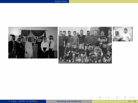
Applications
Figure 7: Output of our face detector on a number of test images from the MIT+CMU test set.
Figure 6: ROC curve for our face detector on the
MIT+CMU test set. The detector was run using a step size
of 1.0 and starting scale of 1.0 (75,081,800 sub-windows
scanned).
have broader application in computer vision and image pro-
cessing.
Finally this paper presents a set of detailed experiments
on a difficult face detection dataset which has been widely
studied. This dataset includes faces under a very wide range
of conditions including: illumination, scale, pose, and cam-
era variation. Experiments on such a large and complex
dataset are difficult and time consuming. Nevertheless sys-
tems which work under these conditions are unlikely to be
brittle or limited to a single set of conditions. More impor-
tantly conclusions drawn from this dataset are unlikely to
be experimental artifacts.
References
[1] Y. Amit, D. Geman, and K. Wilder. Joint induction of shape
features and tree classifi ers, 1997.
[2] Anonymous. Anonymous. In Anonymous, 2000.
[3] F. Crow. Summed-area tables for texture mapping. In
Proceedings of SIGGRAPH, volume 18(3), pages 207–212,
1984.
[4] F. Fleuret and D. Geman. Coarse-to-fi ne face detection. Int.
J. Computer Vision, 2001.
[5] William T. Freeman and Edward H. Adelson. The design
and use of steerable fi lters. IEEE Transactions on Pattern
Analysis and Machine Intelligence, 13(9):891–906, 1991.
[6] Yoav Freund and Robert E. Schapire. A decision-theoretic
generalization of on-line learning and an application to
boosting. In Computational Learning Theory: Eurocolt ’95,
pages 23–37. Springer-Verlag, 1995.
[7] H. Greenspan, S. Belongie, R. Gooodman, P. Perona, S. Rak-
shit, and C. Anderson. Overcomplete steerable pyramid fi l-
ters and rotation invariance. In Proceedings of the IEEECon-
ference on Computer Vision and Pattern Recognition, 1994.
[8] L. Itti, C. Koch, and E. Niebur. A model of saliency-based
visual attention for rapid scene analysis. IEEE Patt. Anal.
Mach. Intell., 20(11):1254–1259, November 1998.
[9] Edgar Osuna, Robert Freund, and Federico Girosi. Training
support vector machines: an application to face detection.
In Proceedings of the IEEE Conference on Computer Vision
and Pattern Recognition, 1997.
[10] C. Papageorgiou, M. Oren, and T. Poggio. A general frame-
work for object detection. In International Conference on
Computer Vision, 1998.
[11] D. Roth, M. Yang, and N. Ahuja. A snowbased face detector.
In Neural Information Processing 12, 2000.
[12] H. Rowley, S. Baluja, and T. Kanade. Neural network-based
face detection. In IEEE Patt. Anal. Mach. Intell., volume 20,
pages 22–38, 1998.
[13] R. E. Schapire, Y. Freund, P. Bartlett, and W. S. Lee. Boost-
ing the margin: a new explanation for the effectiveness of
voting methods. Ann. Stat., 26(5):1651–1686, 1998.
[14] Robert E. Schapire, Yoav Freund, Peter Bartlett, and
Wee Sun Lee. Boosting the margin: A new explanation for
the effectiveness of voting methods. In Proceedings of the
Fourteenth International Conference on Machine Learning,
1997.
[15] H. Schneiderman and T. Kanade. A statistical method for 3D
object detection applied to faces and cars. In International
Conference on Computer Vision, 2000.
8
J. Corso (SUNY at Buffalo) Boosting and AdaBoost 57 / 62
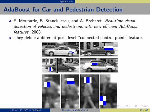
Applications
AdaBoost for Car and Pedestrian Detection
F. Moutarde, B. Stanciulescu, and A. Breheret. Real-time visualdetection of vehicles and pedestrians with new efficient AdaBoostfeatures. 2008.They define a different pixel level “connected control point” feature.
Abstract— This paper deals with real-time visual detection,
by mono-camera, of objects categories such as cars and
pedestrians. We report on improvements that can be obtained
for this task, in complex applications such as advanced driving
assistance systems, by using new visual features as adaBoost
weak classifiers. These new features, the “connected control-
points” have recently been shown to give very good results on
real-time visual rear car detection. We here report on results
obtained by applying these new features to a public lateral car
images dataset, and a public pedestrian images database. We
show that our new features consistently outperform previously
published results on these databases, while still operating fast
enough for real-time pedestrians and vehicles detection.
I. INTRODUCTION AND RELATED WORK
UTONOMOUS vehicles, as well as most Advanced
Driving Assistance System (ADAS) functions, require
real-time perception analysis. This environment perception
can be done using various sensors such as lidars, radars,
ultrasonic devices, etc… However, compared to other
sensors, visual perception can provide very rich information
for very low equipment costs, if an abstract enough scene
analysis can be conducted in real-time.
One of the key bricks required for such an automated
scene analysis is efficient visual detection of most common
moving objects in car environment: vehicles and pedestrians.
Many techniques have been proposed for visual object
detection and classification (see eg [10] for a review of some
of the state-of-the-art methods for pedestrian detection,
which is the most challenging). Of the various machine-
learning approaches applied to this problem, only few are
able to process videos in real-time. Among those last ones,
the boosting algorithm with feature selection was
successfully extended to machine-vision by Viola & Jones
[4][5]. The adaBoost algorithm was introduced in 1995 by
Y. Freund and R. Shapire [1][2], and its principle is to build
a strong classifier, assembling weighted weak classifiers,
those being obtained iteratively by using successive
weighting of the examples in the training set.
Most published works using adaBoost for visual object
class detection are using the Haar-like features initially
proposed by Viola & Jones for face and pedestrian detection.
Manuscript received June 10, 2008.
F. Moutarde, B. Stanciulescu and A. Breheret are all with the Robotics
Laboratory of Mines ParisTech, 60 Bd St Michel, 75006 Paris, FRANCE
(33-1-40.51.92.92, {Fabien.Moutarde,Bogdan.Stanciulescu}@ensmp.fr).
Fig.1: Viola &Jones Haar-like features
These weak classifiers compute the absolute difference
between the sum of pixel values in red and blue areas (see
figure 1), with the respect of the following rule:
if ThresholdBAreaAArea >! )()( then True
else False
Fig. 2: Some examples of adaBoost-selected Viola-Jones features for
car detection (top) and pedestrian detection (bottom).
However, the adaBoost outcome may strongly depend on the
family of features from which the weak classifiers are drawn.
But rather few investigations have been done on using other
kinds of features with adaBoost: Zhu et al. in [13] defined
and successfully applied adaBoost features directly inspired
from the Histogram of Oriented Gradient (HOG) approach
initially proposed (combined with SVM) by Dalal [12];
Baluja et al. in [14] and Leyrit et al. in [15] both use pixel-
comparison-based feature very similar, although simplified,
to our lab’s control-points approach ([6][7][8][9]); very
recently Pettersson et al. in [16] proposed efficient gradient-
histogram-based features inspired from HOG.
Real-time visual detection of vehicles and pedestrians
with new efficient adaBoost features
Fabien Moutarde, Bogdan Stanciulescu and Amaury Breheret
A
J. Corso (SUNY at Buffalo) Boosting and AdaBoost 58 / 62

Applications
II. CONTROL-POINTS ADABOOST FEATURES
Several years ago, Abramson & Steux [6][7] proposed an
original set of features, the control-points, for faster and
more illumination-independant adaBoost classifiers.
These features operate directly at pixel level (at one
among 3 different possible resolutions) and are illumination-
independent. Each of these features can be computed by only
a few pixel comparisons, which makes them extremely fast,
thus providing very good real-time performances for the
resulting detector. Arbitrary points are divided in two
groups, one called the positive set and the second called the
negative set. Examples are classified as positive, if the
following condition applies:
{ } { } VNjPNiP ji >=!= !
!
++
),...,1,max(),...,1,min(
OR
{ } { } VNiPNjP ij >=!= ++
!
!),...,1,max(),...,1,min(
V is the minimum separation threshold between the two
point groups, Pi+ a point from the positive group, Pj
- a point
from the negative group, and N+ and N- the number of points
in the respective groups.
Fig. 3a: Positive-classified example with respect
to the threshold V.
Fig. 3b: Negative-classified example.
In a linear representation of the pixel values, an example
is classified as positive if the two point groups are separated
by at least the value of threshold V (see figure 3a). Negative
examples are those that do not respect this characteristic:
values of the control-points of the two groups are interleaved
(see figure 3b).
One can see on the figure 4 some examples of control-
points features acting on vehicle or pedestrian detection.
Each feature operates at either full-, half- or quarter-
resolution of the minimal detection window size (80x32 for
the lateral car case, and 18x36 for the pedestrian case). An
examined image or sub-window is thus resized to those 3
resolutions before the features are applied.
On the upper-left example of figure 4, the feature will
respond positively if the 2 pixels values (on the correctly
resized image) corresponding to the 2 white squares all have
higher luminance (with margin " V) than all 3 pixels values
corresponding to the 3 red squares (or opposite). This
particular feature can therefore be interpreted as detecting
some usual contrast between the car itself and region just
below, with shadow and dark tyres. Similarly, the lower-left
feature seems to detect some contrast between pedestrian
center and the background. Such interpretation of selected
control-points features is not always very clear, however.
AdaBoost requires a ”weak learner”, i.e. an algorithm
which will select and provide, for each adaBoost step, a
”good” feature (i.e. with a ”low-enough” weighted error
measured on the training set). The weak learner used by
Viola and Jones is just an exhaustive search of all
~180,000 possible features in their set of features. But as our
control-point family features is absolutely huge (there are
more than 1035
of them for a 36 ! 36 detection window size),
a systematic full search is definitely not possible. We
therefore use as weak learner a genetic-like heuristic search
in feature space: an evolutionary hill-climbing described in
more details in [8].
The core of our heuristic search weak-learner is to define
specific mutations adapted to the feature-type, and apply
them to a population of initially random features. A single
mutation of one control-points feature typically consists in
adding, moving, or removing one of the points, changing
working resolution, or modifying the value of threshold V.
When evolution provides no more improvement, the best
feature of the population is selected and the weak-learner
returns it to be added as the next adaBoost feature.
Fig. 4: Some examples of adaBoost-selected Control-Points features for
car detection (top) and pedestrian detection (bottom line). Some features
operate at full resolution of detection window (eg rightmost bottom), while
others work on half-resolution (eg leftmost bottom), or even at quarter-
resolution (third on bottom line).
J. Corso (SUNY at Buffalo) Boosting and AdaBoost 59 / 62

Applications
best Area Under Curve with 0.91, instead of 0.88)
outperforms both our usual simple control-points, and Haar-
like features.
Figure 7 shows some detection results on test wider-field
images by our connected-control-points adaBoost classifier.
These illustrate the robustness to at least moderate occlusion,
of classifiers built with our new features.
Fig. 7: Some detection results with our connected-control-points adaBoost
classifier, which illustrates its robustness to at least moderate occlusion.
If we compare detectors with similar computation loads
(in this particular setup, control-points features operate ~ 8
times faster than our implementation of ViolaJones Haar-like
features), then the superiority of our new connected control-
points features over Haar-like features is even clearer (see
figure 7). It should be noted however that our ViolaJones
classifiers were obtained using the same heuristic weak-
learner as for control-points (with adapted mutation
operator), rather than usual full-search which would anyway
have been prohibitively long for a 80x32 detection window
size.
PR_lateralCar_multiScale
0,6
0,65
0,7
0,75
0,8
0,85
0,9
0,95
1
0 0,1 0,2 0,3 0,4 0,5 0,6 0,7 0,8 0,9 11-precision
recall
connectedCP800_80x32
VJ100_80x32
Fig. 7: Precision-recall for adaBoost lateral car detection, when comparing
detectors with similar computation loads. At equivalent computation time,
our new connected-control-points features clearly outperform ViolaJone
Haar-like features.
B. Pedestrians database
The pedestrian database comprises 3 training sets and 2
test sets (each one of the 5 sets with 4800 positive examples
and 5000 negative ones). As suggested in [10], 3
independent trainings were conducted on unions of 2 of the 3
training sets, and the evaluation was done on the 2 test sets,
producing a total of 6 evaluations, to be averaged, for each
feature type. In each training, 2000 boosting steps were
allowed, therefore producing adaBoost detectors assembling
2000 weak-classifiers.
Fig. 9: Averaged ROC curves for adaBoost pedestrian classifiers obtained
with various feature families
As one can see in figure 9, the classifiers obtained with
the new “connected control-points” features have by far the
best classification results. The Viola-Jones performs rather
poorly, even when compared to “ordinary control-points”.
We also compared the performance of our new classifier
to the Viola-Jones classifier performance reported in [10],
which was obtained with openCV implementation. As can be
seen on figure 10, our “connected control-points” pedestrian
classifier has a significantly better performance, which
confirms the results obtained with our own implementation
(with which we did not use cascade for our comparisons).
J. Corso (SUNY at Buffalo) Boosting and AdaBoost 60 / 62
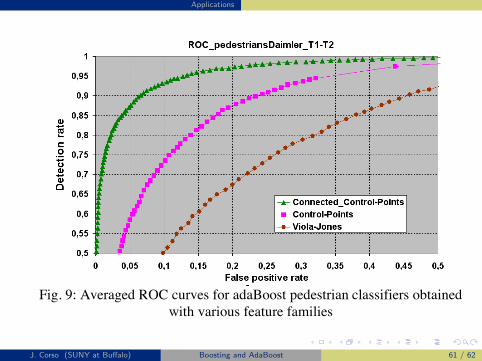
Applications
best Area Under Curve with 0.91, instead of 0.88)
outperforms both our usual simple control-points, and Haar-
like features.
Figure 7 shows some detection results on test wider-field
images by our connected-control-points adaBoost classifier.
These illustrate the robustness to at least moderate occlusion,
of classifiers built with our new features.
Fig. 7: Some detection results with our connected-control-points adaBoost
classifier, which illustrates its robustness to at least moderate occlusion.
If we compare detectors with similar computation loads
(in this particular setup, control-points features operate ~ 8
times faster than our implementation of ViolaJones Haar-like
features), then the superiority of our new connected control-
points features over Haar-like features is even clearer (see
figure 7). It should be noted however that our ViolaJones
classifiers were obtained using the same heuristic weak-
learner as for control-points (with adapted mutation
operator), rather than usual full-search which would anyway
have been prohibitively long for a 80x32 detection window
size.
PR_lateralCar_multiScale
0,6
0,65
0,7
0,75
0,8
0,85
0,9
0,95
1
0 0,1 0,2 0,3 0,4 0,5 0,6 0,7 0,8 0,9 11-precision
recall
connectedCP800_80x32
VJ100_80x32
Fig. 7: Precision-recall for adaBoost lateral car detection, when comparing
detectors with similar computation loads. At equivalent computation time,
our new connected-control-points features clearly outperform ViolaJone
Haar-like features.
B. Pedestrians database
The pedestrian database comprises 3 training sets and 2
test sets (each one of the 5 sets with 4800 positive examples
and 5000 negative ones). As suggested in [10], 3
independent trainings were conducted on unions of 2 of the 3
training sets, and the evaluation was done on the 2 test sets,
producing a total of 6 evaluations, to be averaged, for each
feature type. In each training, 2000 boosting steps were
allowed, therefore producing adaBoost detectors assembling
2000 weak-classifiers.
Fig. 9: Averaged ROC curves for adaBoost pedestrian classifiers obtained
with various feature families
As one can see in figure 9, the classifiers obtained with
the new “connected control-points” features have by far the
best classification results. The Viola-Jones performs rather
poorly, even when compared to “ordinary control-points”.
We also compared the performance of our new classifier
to the Viola-Jones classifier performance reported in [10],
which was obtained with openCV implementation. As can be
seen on figure 10, our “connected control-points” pedestrian
classifier has a significantly better performance, which
confirms the results obtained with our own implementation
(with which we did not use cascade for our comparisons).
J. Corso (SUNY at Buffalo) Boosting and AdaBoost 61 / 62

References
Sources
These slides have made extensive use of the following sources.
Y.Freund and R.E. Schapire. A Decision-Theoretic Generalization of On-lineLearning and an Application to Boosting. Journal of Computer and SystemScience, 55(1):119139, 1997.
R.E. Schapire. The boosting approach to machine learning: an overview. InMSRI Workshop on Nonlinear Estimation and Classification, 2002.
Schapire’s NIPS Tutorial http://nips.cc/Conferences/2007/Program/schedule.php?Session=Tutorials
P.Viola and M.Jones. Rapid object detection using a boosted cascade ofsimple features. In Proceedings of IEEE Conference on Computer Vision andPattern Recognition, 2001.
P.Viola and M.Jones. Fast and Robust Classification Using AsymmetricAdaBoost and a Detector Cascade. In Proceedings of Neural InformationProcessing Systems (NIPS), 2002.
SC Zhu’s slides for AdaBoost (UCLA).
J. Corso (SUNY at Buffalo) Boosting and AdaBoost 62 / 62