actuarial and financial mathematics conference - ugent · koninklijke vlaamse academie van belgie...
TRANSCRIPT

KONINKLIJKE VLAAMSE ACADEMIE VAN BELGIE
VOOR WETENSCHAPPEN EN KUNSTEN
ACTUARIAL AND FINANCIAL
MATHEMATICS CONFERENCE Interplay between Finance and Insurance
February 5-6, 2009
Michèle Vanmaele, Griselda Deelstra, Ann De Schepper,
Jan Dhaene & Paul Van Goethem (Eds.)
CONTACTFORUM


KONINKLIJKE VLAAMSE ACADEMIE VAN BELGIE
VOOR WETENSCHAPPEN EN KUNSTEN
ACTUARIAL AND FINANCIAL
MATHEMATICS CONFERENCE Interplay between Finance and Insurance
February 5-6, 2009
Michèle Vanmaele, Griselda Deelstra, Ann De Schepper,
Jan Dhaene & Paul Van Goethem (Eds.)
CONTACTFORUM

Handelingen van het contactforum "Actuarial and Financial Mathematics Conference. Interplay between Finance and Insurance" (5-6 februari 2009, hoofdaanvrager: Prof. M. Vanmaele, UGent) gesteund door de Koninklijke Vlaamse Academie van België voor Wetenschappen en Kunsten. Afgezien van het afstemmen van het lettertype en de alinea’s op de richtlijnen voor de publicatie van de handelingen heeft de Academie geen andere wijzigingen in de tekst aangebracht. De inhoud, de volgorde en de opbouw van de teksten zijn de verantwoordelijkheid van de hoofdaanvrager (of editors) van het contactforum.
KONINKLIJKE VLAAMSE ACADEMIE VAN BELGIE VOOR WETENSCHAPPEN EN KUNSTEN Paleis der Academiën Hertogsstraat 1 1000 Brussel
© Copyright 2009 KVAB D/2009/0455/13
ISBN 9789065690524
Niets uit deze uitgave mag worden verveelvoudigd en/of openbaar gemaakt door middel van druk, fotokopie, microfilm of op welke andere wijze ook zonder voorafgaande schriftelijke toestemming van de uitgever. No part of this book may be reproduced in any form, by print, photo print, microfilm or any other means without written permission from the publisher. Printed by Universa Press, 9230 Wetteren, Belgium
KONINKLIJKE VLAAMSE ACADEMIE VAN BELGIE
VOOR WETENSCHAPPEN EN KUNSTEN
Actuarial and Financial Mathematics Conference Interplay between finance and insurance
CONTENTS
Short Course The world of VG.................................................................................…….……................ 3
W. Schoutens Contri buted talks Death bonds with stochastic force of mortality…………….....……….....………....…..... 57
F. Menoncin Generic pricing of FX, inflation and stock options under stochastic interest rates and stochastic volatility............................................................................................………......
71
A. van Haastrecht, A. Pelsser Extended Abstracts / Poster session Vanna-Volga methods applied to FX derivative: from theory to market practice............... 87 F. Bossens, G. Deelstra, G. Rayée, N. Skantzos An analysis of the underwriting cycle for non-life insurance companies.....…………....... 89 R.R. Cerchiara, F. Lamantia Implied Lévy volatility...................... ……...…………………….…….............................. 91 J.M. Corcuera, F. Guillaume, P. Leoni, W. Schoutens A geostatical approach for dynamic life tables. The effect of mortality on remaining lifetime and annuities....................................................................................................…...
93
A. Debon, F. Martínez-Ruiz, F. Montes Pricing and hedging Asian basket spread options....................................................…..….. 95 G. Deelstra, A. Petkovic, M. Vanmaele

Risk indifference pricing and backward stochastic differential equations........................ 97 X. De Scheemaekere Syndicated secured loan derivatives: modelling of LCDS and pricing of LCDX tranches 99 P. Dobránszky, W. Schoutens Portfolio insurance, is it true that complexity leads to better performances?………….... 101 E.M. Duarte, J.A. Soares da Fonseca
Funding of a hybrid pension scheme ……...…………………….……............................ 103 D. Gómez-Hernández, I. Owadally, S. Haberman Non-parametric estimation for multivariate compound Poisson processes and goodness-of-fit testing.......................................................................................................
105
M. Schicks
KONINKLIJKE VLAAMSE ACADEMIE VAN BELGIE
VOOR WETENSCHAPPEN EN KUNSTEN
Actuarial and Financial Mathematics Conference Interplay between finance and insurance
PREFACE On February 5 and 6, the contactforum “Actuarial and Financial Mathematics Conference” (AFMathConf2009) took place in the buildings of the Royal Flemish Academy of Belgium for Science and Arts in Brussels. The main goal of this conference is to strengthen the ties between researchers in actuarial and financial mathematics from Belgian universities and from abroad on the one side, and professionals of the banking and insurance business on the other side. The conference attracted more than 100 participants from 14 different countries, illustrating the large interest from academia as well as from practitioners. For the 2009 edition, we slightly changed the formula: next to guest speakers and contributions, the conference also included two short courses and a poster session. During the first day, we welcomed two invited speakers: Arne Sandström (Swedish Insurance Foundation, Sweden) and Wim Schoutens (Katholieke Universiteit Leuven, Belgium), who gave first-class short courses on Solvency II and on Lévy processes. On the second day, all attendants had the opportunity to listen to four guest speakers: Ernst Eberlein (University of Freiburg, Germany), Damiano Brigo (Imperial College London & Fitch Solutions, UK and member of the Advisory Board of AMaMeF), Michel Denuit (Université catholique de Louvain, Belgium) and Anna Rita Bacinello (University of Trieste, Italy), and to four more contributions from Alexander van Haastrecht (University of Amsterdam & Delta Lloyd, the Netherlands), Roger Laeven (Tilburg University, the Netherlands), Francesco Menoncin (Università di Brescia, Italy) and Beatrice Acciaio (Vienna University of Technology, Austria). We thank them all for their enthusiasm and their interesting presentations which made the conference a great success. The present proceedings give a nice overview of the activities at the conference. They contain the lecture notes for one of the short courses, two papers corresponding to contributed talks, and ten abstracts of posters presented during the poster sessions on both conference days. We are much indebted to the members of the scientific committee, Freddy Delbaen (ETH Zurich, Switzerland), Rob Kaas (University of Amsterdam, the Netherlands), Ragnar Norberg (London School of Economics, UK), Bernt Øksendal (University of Oslo, Norway), Antoon Pelsser (University of Amsterdam, the Netherlands), Noel Veraverbeke (Universiteit Hasselt, Belgium) and Griselda Deelstra (Université Libre de Bruxelles & Vrije Universiteit Brussel, Belgium), for the excellent scientific support. We also thank Wouter Dewolf (Ghent University, Belgium), for the administrative work.

We cannot forget our sponsors, who made it possible to organise this event in a very agreeable and inspiring environment. We are very grateful to the Royal Flemish Academy of Belgium for Science and Arts, the Research Foundation Flanders (FWO), the Scientific Research Network (WOG) “Fundamental Methods and Techniques in Mathematics”, le Fonds de la Recherche Scientific (FNRS), the KULeuven Fortis Chair in Financial and Actuarial Risk Management, the IAP programme IAP P6/07 (Belgian Scientific Policy), and the ESF program “Advanced Mathematical Methods in Finance” (AMaMeF). The success of the meeting encourages us to go on with the organisation of this contactforum. We are sure that continuing this event will provide more opportunities to facilitate the exchange of ideas and results in our fascinating research field. The editors: Griselda Deelstra Ann De Schepper Jan Dhaene Paul Van Goethem Michèle Vanmaele The other members of the organising committee: Pierre Devolder Steven Vanduffel Martine Van Wouwe David Vyncke

SHORT COURSE
1

2

THE WORLD OF VG
Wim Schoutens
Department of Mathematics, Katholieke Universiteit Leuven, Celestijnenlaan 200 B, B-3001 Leu-ven, BelgiumEmail: [email protected]
Abstract
This note is a practical guide to the use of jump processes in financial modelling. Jumpsand extreme events are crucial stylized features and are essential in the modelling of volatilemarkets. The recent turmoil in the markets have illustrated once more the need for morerefined models. We illustrate how the classical models (driven by Brownian motions, cfr.Black-Scholes settings) can be significantly improved by considering the more flexible classof Levy processes. By doing this extreme event and jumps are introduced in the models anda more reliable pricing and a better assessment of the risk presents can be made. Besides thesetting up of the theoretical framework, many attention is paid to the practical aspects. We dealwith the basic vanilla pricing, the calibration of the model to given implied volatility surfacesand exotic option pricing by Monte-Carlo methods.
1. THE BLACK-SCHOLES MODEL
This section overviews the most basic and well-known continuous-time, continuous-variable stochas-tic model for stock prices. An understanding of this is the first step to the understanding of thepricing of options in a more advanced setting.
1.1. The Normal Distribution
The Normal distribution, Normal(µ, σ2), is one of the most important distributions in many areas.It lives on the real line, has meanµ ∈ R and varianceσ2 > 0. Its characteristic function is givenby
φNormal(u; µ, σ2) = exp(iuµ) exp
(
−σ2u2
2
)
3

4 W. Schoutens
and the density function is given as
fNormal(x; µ, σ2) =1√
2πσ2exp
(
−(x − µ)2
2σ2
)
.
In Figure 1, one sees the typical bell-shaped curve of the density of a standard normal density.
−3 −2 −1 0 1 2 30
0.05
0.1
0.15
0.2
0.25
0.3
0.35
0.4
0.45
0.5
Density Function of a Standard Normal Distribution
Figure 1: Density of a Standard Normal Distribution
The Normal(µ, σ2) distribution is symmetric around its mean, and has always a kurtosis equalto 3:
Normal(µ, σ2)mean µvariance σ2
skewness 0kurtosis 3
We will denote by
N(x) =
∫ x
−∞
fNormal(u; 0, 1)du (1)
the cumulative probability distribution function for a variable that is standard normally distributed(Normal(0, 1)). This special function is available in most mathematical software packages.
1.2. Brownian Motion
The big brother of the Normal distribution is the Brownian motion. Brownian motion is the dy-namic counterpart – where we work with evolution in time – of its static counterpart, the Normaldistribution. Both arise from the central limit theorem. Intuitively, it tells us that the suitable nor-malized sum of many small independent random variables is approximately normally distributed.

The World of VG 5
These results explain the ubiquity of the Normal distribution in a static context. If one works in adynamic setting, i.e. with stochastic processes, Brownian motion appears in the same manner.
1.2.1. THE HISTORY OFBROWNIAN MOTION
The history of Brownian motion dates back to 1828, when the Scottish botanist Robert Brownobserved pollen particles in suspension under a microscope and observed that they were in constantirregular motion. By doing the same with particles of dust, he was able to rule out that the motionwas due to pollen being ”alive”.
In 1900 L. Bachelier considered Brownian motion as a possible model for stock market prices.Bachelier’s model was his thesis. At that time the topic was not thought worthy of study.
In 1905 Albert Einstein considered Brownian motion as a model of particles in suspension.Einstein observed that, if the kinetic theory of fluids was right, then the molecules of water wouldmove at random and so a small particle would receive a random number of impacts of randomstrength and from random directions in any short period of time. Such a bombardment wouldcause a sufficiently small particle to move in exactly the way described by Brown. Einstein alsoused it to estimate Avogadro’s number.
In 1923 Norbert Wiener defined and constructed Brownian motion rigorously for the first time.The resulting stochastic process is often called the Wiener process in his honor.
It was with the work of [104] that Brownian motion reappeared as a modeling tool in finance.
1.2.2. DEFINITION
A stochastic processX = Xt, t ≥ 0 is astandard Brownian motionon some probability space(Ω,F , P ), if
1. X0 = 0 a.s.
2. X has independent increments.
3. X has stationary increments.
4. Xt+s−Xt is normally distributed with mean 0 and variances > 0: Xt+s−Xt ∼ Normal(0, s).
We shall henceforth denote standard Brownian motion byW = Wt, t ≥ 0 (W for Wiener).Note that the second item in the definition implies that Brownian motion is a Markov process.Moreover Brownian motion is the basic example of a Levy process (see [113]).
In the above, we have defined Brownian motion without reference to a filtration. Without othernotice, we will always work with the natural filtrationF = F
W = Ft, 0 ≤ t ≤ T of W . We havethat Brownian motion is adapted with respect to this filtration and that incrementsWt+s − Wt areindependent ofFt.

6 W. Schoutens
1.2.3. RANDOM-WALK APPROXIMATION OF BROWNIAN MOTION
No construction of Brownian motion is easy. We take the existence of Brownian motion forgranted. To gain some intuition on its behaviour, it is good to compare Brownian motion witha simple symmetric random walk on the integers. More precisely, letX = Xi, i = 1, 2, . . . bea series of independent and identically distributed random variables withP (Xi = 1) = P (Xi =−1) = 1/2. Define the simple symmetric random walkZ = Zn, n = 0, 1, 2, . . . asZ0 = 0 andZn =
∑ni=1 Xi, n = 1, 2, . . . . Rescale this random walk asYk(t) = Z⌊kt⌋/
√k, where⌊x⌋ is the
integer part ofx. Then from the Central Limit Theorem,Yk(t) → Wt ask → ∞, with convergencein distribution (or weak convergence).
In Figure 2, one sees a realization of the standard Brownian motion. In Figure 3, one sees the
0 0.1 0.2 0.3 0.4 0.5 0.6 0.7 0.8 0.9 1−0.8
−0.6
−0.4
−0.2
0
0.2
0.4
0.6
0.8
1Standard Brownian Motion
Figure 2: A sample path of a standard Brownian motion
random-walk approximation of the standard Brownian motion. The processYk = Yk(t), t ≥ 0is shown fork = 1 (i.e. the symmetric random walk),k = 3, k = 10 andk = 50. Clearly, onesees theYk(t) → Wt.
1.2.4. PROPERTIES
Next, we look at some of the classical properties of Brownian motion.
Martingale Property Brownian motion is one of the most simple examples of a martingale. Wehave for all0 ≤ s ≤ t,
E[Wt|Fs] = E[Wt|Ws] = Ws.
We also mention that one has:E[WtWs] = mint, s.
Path Properties One can proof that Brownian motion has continuous paths, i.e.Wt is a contin-uous function oft. However the paths of Brownian motion are very erratic. They are for example

The World of VG 7
0 10 20 30 40 50−10
−5
0
5
10k=1
0 10 20 30 40 50−10
−5
0
5
10k=3
0 10 20 30 40 50−10
−5
0
5
10k=10
0 10 20 30 40 50−10
−5
0
5
10k=50
Figure 3: Random walk approximation for standard Brownian motion
nowhere differentiable. Moreover, one can prove also that the paths of Brownian motion are ofinfinite variation, i.e. their variation is infinite on every interval.
Another property is that for a Brownian motionW = Wt, t ≥ 0, we have that
P (supt≥0
Wt = +∞ and inft≥0
Wt = −∞) = 1.
This result tells us that the Brownian path will keep oscillating between positive and negativevalues.
Scaling Property There is a well-known set of transformations of Brownian motion which pro-duce another Brownian motion. One of this is the scaling property which says that ifW = Wt, t ≥0 is a Brownian motion, then also for everyc 6= 0,
W = Wt = cWt/c2 , t ≥ 0 (2)
is a Brownian motion.
1.3. Geometric Brownian Motion
Now that we have Brownian motionW , we can introduce an important stochastic process for us,a relative of Brownian motion –geometric Brownian motion.
In the Black-Scholes model, one models the time evolution of a stock priceS = St, t ≥ 0as follows. Consider howS will change in some small time interval from the present timet to atime t + ∆t in the near future. Writing∆St for the changeSt+∆t − St, the return in this interval is

8 W. Schoutens
∆St/St. It is economically reasonable to expect this return to decompose into two components, asystematicpart and arandompart.
Let us first look at the systematic part. One assumes that the stock’s expected return over aperiod is proportional with the length of the period considered. This means that in a short intervalof time [St, St+∆t] of length∆t, the expected increase inS is given byµSt∆t, whereµ is someparameter representing the mean rate of the return of the stock. In other words, the deterministicpart of the stock return is modeled byµ∆t.
A stock price fluctuates stochastically, and a reasonable assumption is that the variance of thereturn over the interval of time[St, St+∆t] is proportional to the length of the interval. So, therandom part of the return is modeled byσ∆Wt, where∆Wt represents the (normally distributed)noise term (with variance∆t) driving the stock price dynamics, andσ > 0 is the parameter whichdescribes how much effect the noise has – how much the stock price fluctuates. In total the varianceof the return equalsσ2∆t. Thusσ governs how volatile the price is, and is called thevolatility ofthe stock. Putting this together, we have
∆St = St(µ∆t + σ∆Wt), S0 > 0.
In the limit, as∆t → 0, we have the stochastic differential equation (SDE)
dSt = St(µdt + σdWt), S0 > 0. (3)
The stochastic differential equation above has the unique solution
St = S0 exp
((
µ − σ2
2
)
t + σWt
)
.
This (exponential) functional of Brownian motion is called geometric Brownian motion. Note that
log St − log S0 =
(
µ − σ2
2
)
t + σWt
has a Normal(t(µ − σ2/2), σ2t) distribution. ThusSt itself has alognormaldistribution. Thisgeometric Brownian motion model, and the log-normal distribution which it entails, are the basisfor the Black-Scholes model for stock-price dynamics in continuous time.
In Figure 4, one sees the realization of the geometric Brownian motion based on the samplepath of the standard Brownian motion of Figure 2.
1.4. The Black-Scholes Option Pricing Model
In the early 1970s, Fischer Black, Myron Scholes, and Robert Merton made a major breakthroughin the pricing of stock options by developing what has become known as the Black-Scholes model.The model has had huge influence on the way that traders price and hedge options. In 1997, theimportance of the model was recognized when Myron Scholes and Robert Merton were awardedthe Nobel prize for economics. Sadly, Fischer Black died in 1995, otherwise he also would un-doubtedly have been one of the recipients of this prize.
We show how the Black-Scholes model for valuing European call and put options on a stockworks.

The World of VG 9
0 0.1 0.2 0.3 0.4 0.5 0.6 0.7 0.8 0.9 170
80
90
100
110
120
130
140
Geometric Brownian Motion (S0=100; mu=0.05; sigma=0.40)
Figure 4: Sample path of a geometric Brownian motion (S0 = 100, µ = 0.05, σ = 0.40)
1.4.1. THE BLACK -SCHOLES MARKET MODEL
Investors are allowed to trade continuously up to some fixed finite planning horizonT . The uncer-tainty is modeled by a filtered probability space(Ω,F , P ). We assume a frictionless market with2 assets.
The first asset is one without risk (the bank account). Its price process is given byB = Bt =exp(rt), 0 ≤ t ≤ T. The second asset is a risky asset, usually referred to as stock, and whichpays a continuous dividend yieldq ≥ 0. The price process of this stock,S = St, 0 ≤ t ≤ T, ismodeled by geometric Brownian motion:
Bt = exp(rt), St = S0 exp
((
µ − σ2
2
)
t + σWt
)
,
whereW = Wt, t ≥ 0 is standard Brownian motion.Note that, underP , Wt has a Normal(0, t) and thatS = St, t ≥ 0 satisfies the SDE (3). The
parameterµ is reflecting the drift andσ models the volatility;µ andσ are assumed to be constantover time.
We assume as underlying filtration, the natural filtrationF = (Ft) generated byW . Conse-quently, the stock price processS = St, 0 ≤ t ≤ T follows a strictly positive adapted process.We call this market model theBlack-Scholes model. It is a well-established result that the Black-Scholes model is a complete model, that is, every contingent claim can be replicated by a dynamicself-financing trading strategy.
1.4.2. THE RISK-NEUTRAL SETTING
Since the Black-Scholes market model is complete there exists only one equivalent martingalemeasureQ. It is not hard to see that underQ, the stock price is following a Geometric Brownianmotion again (Girsanov theorem). This risk-neutral stock price process has the same volatilityparameterσ, but the drift parameterµ is changed to the continuously compounded risk-free rater

10 W. Schoutens
minus the dividend yieldq:
St = S0 exp
((
r − q − σ2
2
)
t + σWt
)
.
Equivalent, we can say that underQ our stock price processS = St, 0 ≤ t ≤ T is satisfying theSDE:
dSt = St((r − q)dt + σdWt), S0 > 0.
This SDE tells us that in a risk-neutral world the total return from the stock must ber; the dividendsprovide a return ofq, the expected growth rate in the stock price, therefore, must ber − q.
Next, we will calculate European call option prices under this model.
1.4.3. THE PRICING OF OPTIONS UNDER THEBLACK -SCHOLES MODEL
General Pricing Formula By the risk-neutral valuation principle the priceVt at time t, of acontingent claim with payoff functionG(Su, 0 ≤ u ≤ T) is given by
Vt = exp(−(T − t)r)EQ[G(Su, 0 ≤ u ≤ T)|Ft], t ∈ [0, T ]. (4)
Furthermore, if the payoff function is only depending on the timeT value of the stock, i.e.G(Su, 0 ≤ u ≤ T) = G(ST ), then the above formula can be rewritten as (we set for simplicityt = 0):
V0 = exp(−Tr)EQ[G(ST )]
= exp(−Tr)EQ[G(S0 exp((r − q − σ2/2)T + σWT ))]
= exp(−Tr)
∫ +∞
−∞
G(S0 exp((r − q − σ2/2)T + σx))fNormal(x; 0, T )dx.
Black-Scholes PDE If moreoverG(ST ) is a sufficiently integrable function, then the price isalso given byVt = F (t, St), whereF solves theBlack-Scholes partial differential equation
∂
∂tF (t, s) + (r − q)s
∂
∂sF (t, s) +
1
2σ2s2 ∂2
∂s2F (t, s) − rF (t, s) = 0, (5)
F (T, s) = G(s)
This follows from the Feynman-Kac representation for Brownian motion (see e.g. [24]).
Explicit Formula for European Call and Put Options Solving the Black-Scholes partial dif-ferential equation (5) is not always that easy. However, in some cases it is possible to evaluateexplicitly the above expected value in the risk-neutral pricing formula (4).
Take for example an European call on the stock (with price processS) with strike K andmaturityT (soG(ST ) = (ST − K)+). The Black-Scholes formulas for the priceC(K, T ) at timezero of this European call option on the stock (with dividend yieldq) is given by
C(K, T ) = C = exp(−qT )S0N(d1) − K exp(−rT )N(d2),

The World of VG 11
where
d1 =log(S0/K) + (r − q + σ2
2)T
σ√
T, (6)
d2 =log(S0/K) + (r − q − σ2
2)T
σ√
T= d1 − σ
√T , (7)
and N(x) is the cumulative probability distribution function for a variable that is standard normallydistributed (Normal(0, 1)).
From this, one can also easily (via the put-call parity) obtain the priceP (K, T ) of the Europeanput option on the same stock with same strikeK and same maturityT :
P (K, T ) = − exp(−qT )S0N(−d1) + K exp(−rT )N(−d2).
For the call, the probability (under Q) of finishing in the money corresponds with N(d2). Sim-ilarly, the delta (i.e. the change in the value of the option compared with the change in the value ofthe underlying asset) of the option corresponds with N(d1).
2. SHORTFALLS OF BLACK-SCHOLES
Over the last decades the Black-Scholes model
St = S0 exp((µ − σ2/2)t + σWt), t ≥ 0,
whereWt, t ≥ 0 is standard Brownian Motion andσ is the usual volatility, turned out to bevery popular. One should bear in mind however, that this elegant theory hinges on several crucialassumptions. We assume that there are no market frictions, like taxes and transaction costs orconstraints on the stock holding, etc. Moreover, empirical evidence suggests that the classicalBlack-Scholes model does not describe the statistical properties of financial time series very well.
Summarizing we could say that under the Black-Scholes framework the following problemshave serious impact on the modeling of financial assets and the corresponding pricing and hedgingof financial derivatives:
• log-returns under the Black-Scholes model are Normally distributed. However it is observedfrom empirical data that log-returns typically do not behave according to a Normal distribu-tion. They show most of the time negative skewness and excess kurtosis.
• related to the above observation on the log-returns, the Black-Scholes model can not modelrealistically extreme events.
• paths of the stock process under the Black-Scholes model are continuous and show no jumps.However in reality one could say that everything is driven by jumps. Moreover, it are es-pecially the more pronounced jumps that have typically the most impact for the derivativepricing under question.

12 W. Schoutens
• the volatility parameter (the only model parameter of relevance for the pricing of derivatives)is assumed to be constant. However, it has been observed that the volatilities or the parame-ters of uncertainty estimated (or more generally the environment) change stochastically overtime and are clustered.
Next, we will focus on each of the above problems a bit more in detail.
2.1. Normal Returns
In Table 1 we summarize i.a. the empirical mean, standard deviation, skewness and kurtosis for aset of popular indices. The first data set (SP500 (1970-2001)) contains all daily log-returns of theSP500 index over the period 1970-2001. The second data set (*SP500 (1970-2001)) contains thesame data except the exceptional log-return (-0.2290) of the crash on the 19th of October 1987.All other data sets are over the period 1997-1999.
2.1.1. SKEWNESS, KURTOSIS AND FAIT-TAILS
We note that the skewness measures the degree to which a distribution is asymmetric and is definedto be the third moment about the mean, divided by the third power of the standard deviation:
E[(X − µX)3]
Var[X]3/2
For a symmetric distribution (like the Normal(µ, σ2)), the skewness is zero. If a distribution has alonger tail to the left than to the right, it is said to have negative skewness. If the reverse is true,then the distribution has a positive skewness. If we look at the daily log-returns of the differentindices, we observe typically some significant (negative) skewness.
Tail behavior and peakedness are measured by kurtosis, which is defined by
E[(X − µX)4]
Var[X]2.
For the Normal distribution (mesokurtic), the kurtosis is 3. If the distribution has a flatter top(platykurtic), the kurtosis is less than 3. If the distribution has a high peak (leptokurtic), the kurtosisis greater than 3.
We clearly see that our data always gives rise to a kurtosis clearly bigger than 3, indicating thatthe tails of the Normal distribution go much faster to zero than the empirical data suggests and thatthe distribution is much more peaked. So large asset price movements occur more frequently thanin a model with Normal distributed increments. This feature is often referred to asexcess kurtosisor fat tails; it is one of the main reasons for considering asset price processes with jumps. The factthat return distributions are more leptokurtic than the Normal one was already noted by [46].
2.1.2. KERNEL DENSITY ESTIMATION
Next, we look at the empirical density of daily log-returns.

The World of VG 13
Index Mean St.Dev. Skewness KurtosisSP500 (1970-2001) 0.0003 0.0099 -1.6663 43.36*SP500 (1970-2001) 0.0003 0.0095 -0.1099 7.17SP500 (1997-1999) 0.0009 0.0119 -0.4409 6.94Nasdaq-Composite 0.0015 0.0154 -0.5439 5.78DAX 0.0012 0.0157 -0.4314 4.65SMI 0.0009 0.0141 -0.3584 5.35CAC-40 0.0013 0.0143 -0.2116 4.63
Table 1: Mean, standard deviation, skewness and kurtosis of major indices
In order to estimate the empirical density, we make use of kernel density estimators. The goalof density estimation is to approximate the probability density functionf(x) of a random variableX. Assume we haven independent observationsx1, . . . , xn from the random variableX. Thekernel density estimatorfh(x) for the estimation of the densityf(x) at pointx is defined as
fh(x) =1
nh
n∑
i=1
K
(
xi − x
h
)
,
whereK(x) is a so-called kernel function, andh is the bandwidth. We typically work with theso-called Gaussian kernel:K(x) = exp(−x2/2)/
√2π. Other possible kernel functions are the
so-called Uniform, Triangle, Quadratic and cosine kernel function. In the above formula one alsohas to select the bandwidthh. We use with our Gaussian kernel, Silverman’s rule of thumb valueh = 1.06σn−1/5.
In Figure 5, one sees the Gaussian kernel density estimator based on the daily log-returns ofthe SP500 Index over the period 1970 until end 2001. We see a sharp peaked distribution. Thistell us that most of the time stock prices do not move that much; there is a considerable amount ofmass around zero. Also in Figure 5 we plotted the Normal density with meanµ = 0.0003112 andσ = 0.0099 corresponding to the empirical mean and standard deviation of the daily log-returns.
2.1.3. SEMI-HEAVY TAILS
Density plots focus on the center of the distribution, however also the tail behavior is important.Therefore, we show in Figure 5 the log densities, i.e.log fh(x) and the corresponding log of theNormal density. The log-density of a Normal distribution has a quadratic decay, whereas theempirical log-density seems to have a much more linear decay. This feature is typical for financialdata and is often referred to as the semi-heaviness of the tails. We say that a distribution or itsdensity functionf(x) has semi-heavy tails, if the tails of the density function behave as
f(x) ∼ C−|x|ρ− exp(−η−|x|) as x → −∞f(x) ∼ C+|x|ρ+ exp(−η+|x|) as x → +∞,
for someρ−, ρ+ ∈ R andC−, C+, η−, η+ ≥ 0. Equivalently,
log f(x) ∼ A− log |x| − η−|x| as x → −∞log f(x) ∼ B+ log |x| − η+|x| as x → +∞,

14 W. Schoutens
−0.04 −0.03 −0.02 −0.01 0 0.01 0.02 0.03 0.040
10
20
30
40
50
60SP500 (1970−2001) Normal and Gaussian Kernel Density Estimators
KernelNormal
−0.04 −0.03 −0.02 −0.01 0 0.01 0.02 0.03 0.04−2
−1
0
1
2
3
4
SP500 (1970−2001) Normal and Gaussian Kernel log−Densities
KernelNormal
Figure 5: Normal density and Gaussian Kernel estimator of the density of the daily log-returns ofthe SP500 index
for someA−, B+ ∈∈ R and η−, η+ ≥ 0. The log-densities for semi-heavy distributions andapparently also financial returns show a linear behavior of the tails towards infinity.
The Normal distribution with meanµ and varianceσ2 exhibits a quadratic decay near infinityof the logarithm of its probability density function:
log fNormal(x; µ, σ2) = −(x − µ)2
2σ2− log
(
σ√
2π)
∼ − 1
2σ2x2 (8)
asx → ±∞. In conclusion, we clearly see that the Normal distribution leads to a very bad fit.
2.1.4. STATISTICAL TESTING
All the above is confirmed by statistical tests on the Normal hypotheses. A standard and straight-forward way of testing goodness of fit of a distribution can be done with the so-calledχ2-test. Theχ2-test counts the number of sample points falling into certain intervals and compares them withthe expected number under the null hypothesis.
More precisely, suppose we haven independent observationsx1, . . . , xn from the random vari-ableX and we want to test whether these observations follow a law with distributionD, dependingonh parameters which we all estimate by some method. First, make a partitionP = A1, . . . Am

The World of VG 15
of the support (in our caseR) of D. The classesAk can be chosen arbitrarily; we consider classesof equal width.
Let Nk, k = 1, . . . , m be the number of observationsxi falling into the setAk; Nk/n iscalled the empirical frequency distribution. We will compare these numbers with the theoreticalfrequency distributionπk, defined by
πk = P (X ∈ Ak), k = 1, . . . , m,
through the Pearson statistic
χ2 =
m∑
k=1
(Nk − nπk)2
nπk.
If necessary we collapse outer cells, such that the expected valuenπk of observations becomesalways greater than five.
We say a random variableχ2j follows a χ2-distribution withj degrees of freedom if it has a
Gamma(j/2, 1/2) law (see Chapter 5):
E[exp(iuχ2j)] = (1 − 2iu)−j/2.
General theory says that the Pearson statisticχ2 follows (asymptotically) aχ2-distribution withm − 1 − h degrees of freedom.
TheP -value of theχ2 statistic is defined as
P = P (χ2m−1−h > χ2).
In words,P is the probability that values are even more extreme (more in the tail) than our test-statistic. It is clear that very smallP -values lead to a rejection of the null hypotheses, because theyare themselves extreme.P -values not close to zero indicate that the test statistic is not extremeand lead not to a rejection of the hypothesis. To be precise we reject if theP -value is less than ourlevel of significance, which we take equal to0.05.
Next, we calculate theP -value for the same set of indices. Table 2 shows theP -values of thetest-statistics. Similar tests can be found i.a. in [40].
Index PNormal-value Class boundariesSP500 (1970-2001) 0.0000 −0.0300 + 0.0015 i, i = 0, . . . , 40SP500 (1997-1999) 0.0421 −0.0240 + 0.0020 i, i = 0, . . . , 24DAX 0.0366 −0.0225 + 0.0015 i, i = 0, . . . , 30Nasdaq-Comp. 0.0049 −0.0300 + 0.0020 i, i = 0, . . . , 30CAC-40 0.0285 −0.0180 + 0.0012 i, i = 0, . . . , 30SMI 0.0479 −0.0180 + 0.0012 i, i = 0, . . . , 30
Table 2: Normalχ2-test:P -values and class boundaries
We see that the Normal hypothesis is always rejected. Basically we can conclude that theNormal distribution, is not sufficiently flexible to capture all features of the data. We need at leastfour parameters: a location parameter, a scale (volatility) parameter, an asymmetry (skewness)
16 W. Schoutens
parameter and a (kurtosis) parameter describing the decay of the tails. We will see that the Levymodels introduced in the next chapter will have this required flexibility.
We have just seen that the well-mannered bell curve of the Gaussian distribution isn’t so normalat all. Next, we focus a bit more on the impact of this on the extreme events and the correspondingimplications of more fatter tails.
2.2. Jumps and Extreme Events
From the above it should be already clear that the stock market doesn’t behave according to Normallaws. Finance likes it hotter, spicier, more extreme. Indeed, extreme price swings are more likelythan the Black-Scholes incorporates them. This insight is not new. Mandelbrot already elaboratedon it in the sixties, long before the Black-Scholes model was ruling Wall Street (see e.g. [60]).
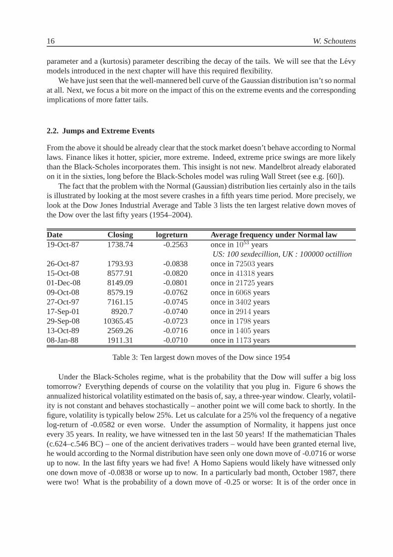
The fact that the problem with the Normal (Gaussian) distribution lies certainly also in the tailsis illustrated by looking at the most severe crashes in a fifth years time period. More precisely, welook at the Dow Jones Industrial Average and Table 3 lists the ten largest relative down moves ofthe Dow over the last fifty years (1954–2004).
Date Closing logreturn Average frequency under Normal law19-Oct-87 1738.74 -0.2563 once in1053 years
US: 100 sexdecillion, UK : 100000 octillion26-Oct-87 1793.93 -0.0838 once in72503 years15-Oct-08 8577.91 -0.0820 once in41318 years01-Dec-08 8149.09 -0.0801 once in21725 years09-Oct-08 8579.19 -0.0762 once in6068 years27-Oct-97 7161.15 -0.0745 once in3402 years17-Sep-01 8920.7 -0.0740 once in2914 years29-Sep-08 10365.45 -0.0723 once in1798 years13-Oct-89 2569.26 -0.0716 once in1405 years08-Jan-88 1911.31 -0.0710 once in1173 years
Table 3: Ten largest down moves of the Dow since 1954
Under the Black-Scholes regime, what is the probability that the Dow will suffer a big losstomorrow? Everything depends of course on the volatility that you plug in. Figure 6 shows theannualized historical volatility estimated on the basis of, say, a three-year window. Clearly, volatil-ity is not constant and behaves stochastically – another point we will come back to shortly. In thefigure, volatility is typically below 25%. Let us calculate for a 25% vol the frequency of a negativelog-return of -0.0582 or even worse. Under the assumption of Normality, it happens just onceevery 35 years. In reality, we have witnessed ten in the last 50 years! If the mathematician Thales(c.624–c.546 BC) – one of the ancient derivatives traders – would have been granted eternal live,he would according to the Normal distribution have seen only one down move of -0.0716 or worseup to now. In the last fifty years we had five! A Homo Sapiens would likely have witnessed onlyone down move of -0.0838 or worse up to now. In a particularly bad month, October 1987, therewere two! What is the probability of a down move of -0.25 or worse: It is of the order once in

The World of VG 17
0.06
0.08
0.1
0.12
0.14
0.16
0.18
0.2
0.22
0.24
0.26Dow Jones Industrial Average − Historic Volatility (1954−2004)
time
histor
ic vo
l
1954 2004
Figure 6:Dow Jones Industrial Average – Historic Volatility (1954–2004)
the 1053 years (in US language: 100 sexdecillion years, UK language: 100000 octillion years). Incontrast, the Big Bangonlyhappened around 15× 109 years ago. The present generation must bereally exceptional that God allowed the Dow to crash in October 1987.
2.2.1. EXPECTED SHORTFALL
Let us focus a bit more on the modeling of extreme values and thetale a tail has to tell. One of themain developer of the theory was the German mathematician, pacifist, and anti-Nazist Emil JuliusGumbel who described the Gumbel distribution in the 1950s (see [55]). Extreme value theory is bynow a well-developed area of statistics and finds applications in many areas of research: besidesfinance, it is/can be used in hydrology, cosmology, insurance, pollution and climatology, geology,etc. A basic reference text is [19].
A risk measure currently gaining in popularity is theexpected shortfall, defined as the expectedexcess over a given (high) level, conditionally on this level being exceeded. The sample versionof the expected shortfall over a certain level is simply the average of the excesses over that level.The expected shortfall over the 1000 largest negative daily log-returns of the Dow are plotted inFigure 7(a). Note that the expected shortfall is increasing with the level: the higher the level beingexceeded, the higher the excess by which it will be exceeded! Once more, this is in sharp contrastwith panel (b) of the same figure: for a Normal sample with the same mean and variance, theexpected shortfall decreases rapidly (note the different axes). In a light-tailed world, given thatyou exceed a high level, you hardly exceed it at all. But in a heavy-tailed world, once you knowyou’ll get hit, you may get hit much harder than expected!

18 W. Schoutens
0 0.02 0.04 0.06 0.08 0.10
0.05
0.1
0.15
0.2
negative logreturn
expe
cted
sho
rtfal
lDow Jones
0.005 0.01 0.015 0.02 0.025 0.03 0.0351
1.5
2
2.5
3
3.5
4
4.5
5x 10
−3
negative logreturn
expe
cted
sho
rtfal
l
Normal sample
(a) (b)
Figure 7: (a)Expected shortfall over 1000 largest negative daily log-return of the Dow (1954–2004).(b) Similarly for a Normal random sample with the same mean and variance.
2.3. No Jumps
Brownian motion has continuous sample paths, whereas in reality prices are driven by jumps. TheBrownian motion needs a substantial amount of time to reach a low barrier, whereas in realityjumps can cause an almost immediate move over the barrier. This has serious impact for exampleon the pricing of barrier products. Because the probability that on the short-term Brownian motionwill hit a barrier far away from its current position is almost zero, prices of down-and-in and up-and-in type of barrier options with short maturities are completely underestimated. Indeed sinceunder Black-Scholes there is almost no possibility that in the short-term the Barrier is hit and thusthe options becomes “in” the price of the product will be extremely low. In reality however, wehave seen above that even in one day extreme movements are possible and that actually the hittingof the barrier is much more likelier. Processes with jumps incorporate this effect and actually makeit possible that even in the next instance the Barrier is trigger. We already here note that this will beespecially crucial in Credit Risk modeling, where it are exactly these extreme default events thatare of importance. Many of the credit derivatives (like for example the Credit Default Swap) canbe seen (under a firm-value model approach) as barrier products with a very low barrier (see forexample [114]).
2.4. Volatility
Another important feature which the Black-Scholes model is missing is the fact that volatility ormore generally the environment is changing stochastically over time.

The World of VG 19
2.4.1. HISTORIC VOLATILITY
It has been observed that the volatilities estimated (or moregeneral the parameters of uncertainty)change stochastically over time. This can be seen for example by looking athistoric volatilities.Historical volatility is a retrospective measure of volatility. It reflects how volatile the asset hasbeen in the recent past. Historical volatility can be calculated for any variable for which historicaldata is tracked.
For the SP500 index, we estimated for every day from 1971 to 2001 the standard deviation ofthe daily log-returns over a one year period preceding the day. In Figure 8, we plot, for every dayin the mentioned period, the annualized standard deviation, i.e. we multiply the simulated standarddeviation with the square root of the number of trading days in one calendar year. Typically, thereare around 250 trading days in one year. This annualized standard deviation is calledthe historicvolatility. In Figure 6 the historical volatility estimated (using a three-years window) was alreadygiven for the Dow Jones Industrial Average. Clearly, we see fluctuations of this historic volatility.Moreover, we see a kind of mean-reversion effect. The peak in the middle of the figures comesfrom the stock market crash on the 19th of October 1987; windows including this day (with anextremal down-move), give rise to very high volatilities.
0.05
0.1
0.15
0.2
0.25
0.3
0.35
0.4Historic Volatility (1year window) SP−500 (1970−2001)
time
volat
ility
2001 1970
Figure 8: Historic Volatilities on SP-500
2.4.2. VOLATILITY CLUSTERS
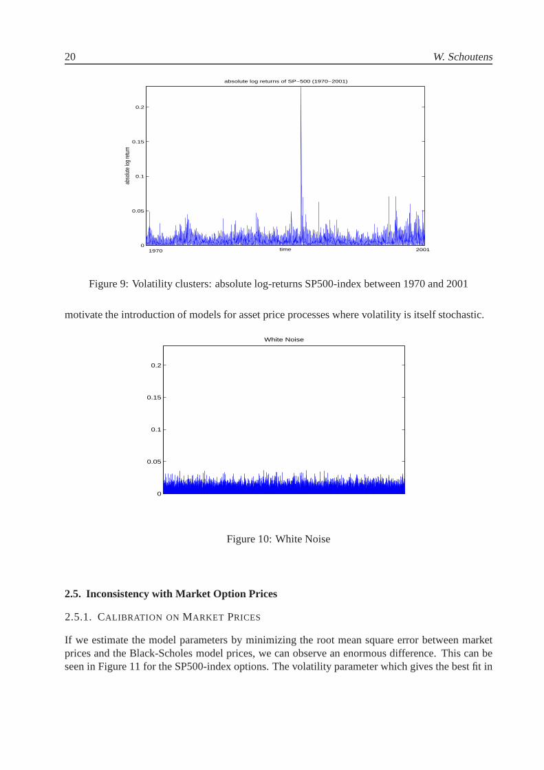
Moreover, there is evidence forvolatility clusters, i.e. there seems to be a succession of periodswith high return variance and with low return variance. This can be seen for example in Fig-ure 9, where the absolute log-returns of the SP500-index over a period of more than 30 years isplotted. One clearly sees that there are periods with high absolute log-returns and periods withlower absolute log-returns. This is in contrast with the picture in Figure 10, where similarly theabsolute value of simulated normal random variables (with the empirical standard deviation of theSP500) are graphed. Here one sees a more homogeneous picture, often referred to as white noise.Large price variations are more likely to be followed by large price variations. These observations
20 W. Schoutens
0
0.05
0.1
0.15
0.2
absolute log returns of SP−500 (1970−2001)
time
abso
lute
log re
turn
1970
2001
Figure 9: Volatility clusters: absolute log-returns SP500-index between 1970 and 2001
motivate the introduction of models for asset price processes where volatility is itself stochastic.
0
0.05
0.1
0.15
0.2
White Noise
Figure 10: White Noise
2.5. Inconsistency with Market Option Prices
2.5.1. CALIBRATION ON MARKET PRICES
If we estimate the model parameters by minimizing the root mean square error between marketprices and the Black-Scholes model prices, we can observe an enormous difference. This can beseen in Figure 11 for the SP500-index options. The volatility parameter which gives the best fit in
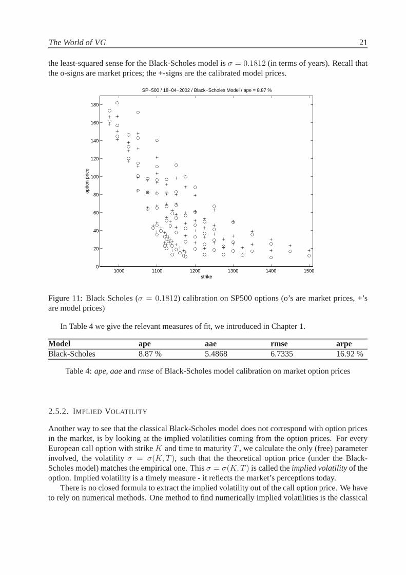
The World of VG 21
the least-squared sense for the Black-Scholes model isσ = 0.1812 (in terms of years). Recall thatthe o-signs are market prices; the +-signs are the calibrated model prices.
1000 1100 1200 1300 1400 15000
20
40
60
80
100
120
140
160
180
SP−500 / 18−04−2002 / Black−Scholes Model / ape = 8.87 %
strike
optio
n pr
ice
Figure 11: Black Scholes (σ = 0.1812) calibration on SP500 options (o’s are market prices, +’sare model prices)
In Table 4 we give the relevant measures of fit, we introduced in Chapter 1.
Model ape aae rmse arpeBlack-Scholes 8.87 % 5.4868 6.7335 16.92 %
Table 4:ape, aaeandrmseof Black-Scholes model calibration on market option prices
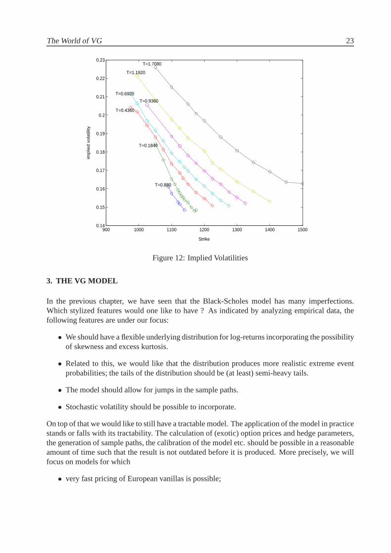
2.5.2. IMPLIED VOLATILITY
Another way to see that the classical Black-Scholes model does not correspond with option pricesin the market, is by looking at the implied volatilities coming from the option prices. For everyEuropean call option with strikeK and time to maturityT , we calculate the only (free) parameterinvolved, the volatilityσ = σ(K, T ), such that the theoretical option price (under the Black-Scholes model) matches the empirical one. Thisσ = σ(K, T ) is called theimplied volatilityof theoption. Implied volatility is a timely measure - it reflects the market’s perceptions today.
There is no closed formula to extract the implied volatility out of the call option price. We haveto rely on numerical methods. One method to find numerically implied volatilities is the classical

22 W. Schoutens
Newton-Raphson iteration procedure. Denote byC(σ) the price of the relevant call option as afunction of volatility. If C is the market price of this option we need to solve the transcendentalequation
C = C(σ) (9)
for σ. We start with some initial value we propose forσ; we denote this starting value withσ0. Interms of years, it turns out that aσ0 around 0.20 performs very well for most common stocks andindices. In general, if we denote byσn the value obtained aftern iteration steps, the next valueσn+1 is given by
σn+1 = σn − C(σn) − C
C ′(σn),
where in the denominatorC ′ refers to the differential with respect toσ of the call price function(this quantity is also referred to as the vega). For the European call option (under Black-Scholes)we have:
C ′(σn) = S0
√TN(d1) = S0
√TN
(
log(S0/K) + (r − q + σ2n
2)T
σn
√T
)
,
whereS0 is the current stock price,d1 as in (6) and N(x) is the cumulative probability distributionof a Normal(0, 1) random variable as in (1).
Next, we bring together for every maturity and strike this volatilityσ in Figure 12, where onesees the so-called volatility surface. Under the Black-Scholes model, allσ’s should be the same;clearly we observe that there is a huge variation in this volatility parameter both in strike as in timeto maturity. One says often there is a volatility smile or skew effect. Again this points to the factthat the Black-Scholes model is not appropriate and the traders already count in this deficiencyinto their prices.
2.5.3. IMPLIED VOLATILITY MODELS
Great care has to be taken by using implied volatilities to price options. Fundamentally, usingimplied volatilities is wrong. Taking different volatilities for different options on the same under-lying asset, give rise to different stochastic models for one asset. Moreover, the situation worsensin case of exotic options. [116] showed that if one tries to find the implied volatilities coming outof exotic options like barrier options (see Chapter 9), there are cases where there are two or eventhree solutions to the implied volatility equation (for the European call option, see Equation (9)).Implied volatilities are thus not unique in these situations. More extremely, if we consider an up-and-out put barrier option, where the strike coincides with the barrier and the risk-free rate equalsthe dividend yield, the Black-Scholes price (for which there is a formula in closed form available)is independent of the volatility. So if the market price happens to coincide with the computedvalue, you can have any implied volatility you want. Otherwise there is no implied volatility.
From this, it should be clear that great caution has to be taken by using European call optionimplied volatilities for exotic options with apparently similar characteristics (like the same strikeprice for example). There is no guarantee that the obtained prices are reflecting true prices.
The World of VG 23
900 1000 1100 1200 1300 1400 15000.14
0.15
0.16
0.17
0.18
0.19
0.2
0.21
0.22
0.23
Strike
imp
lied
vo
latil
ity
T=1.7080
T=1.1920
T=0.9360
T=0.6920
T=0.4360
T=0.1840
T=0.880
Figure 12: Implied Volatilities
3. THE VG MODEL
In the previous chapter, we have seen that the Black-Scholes model has many imperfections.Which stylized features would one like to have ? As indicated by analyzing empirical data, thefollowing features are under our focus:
• We should have a flexible underlying distribution for log-returns incorporating the possibilityof skewness and excess kurtosis.
• Related to this, we would like that the distribution produces more realistic extreme eventprobabilities; the tails of the distribution should be (at least) semi-heavy tails.
• The model should allow for jumps in the sample paths.
• Stochastic volatility should be possible to incorporate.
On top of that we would like to still have a tractable model. The application of the model in practicestands or falls with its tractability. The calculation of (exotic) option prices and hedge parameters,the generation of sample paths, the calibration of the model etc. should be possible in a reasonableamount of time such that the result is not outdated before it is produced. More precisely, we willfocus on models for which
• very fast pricing of European vanillas is possible;

24 W. Schoutens
• calibration of the model on a given implied volatility surface can be performed in a reason-able amount of time;
• fast Monte-Carlo simulation is possible in order to do option pricing of exotic options ofEuropean type;
• finite-difference or other techniques are available to do pricing of American or barrier prod-ucts.
Next, we will start our quest with looking for a more flexible distribution.
3.1. The VG distribution
The Gamma distribution will be an essential building block of the construction of the VarianceGamma (VG) distribution on which we will focus a lot on throughout these notes. We start with isthe definition and some properties of the Gamma distribution.
3.1.1. THE GAMMA DISTRIBUTION
The Gamma distribution is a distribution that lives on the positive real numbers and dependentson two parameters. More precisely, the density function of the Gamma distribution Gamma(a, b)with parametersa > 0 andb > 0 is given by
fGamma(x; a, b) =ba
Γ(a)xa−1 exp(−xb), x > 0.
The density function clearly has a semi-heavy (right) tail; for different parameter values the densityfunction is graphed in Figure 13.
0 1 2 3 4 5 6 7 8 9 100
0.1
0.2
0.3
0.4
0.5
0.6
0.7
0.8
0.9
1Gamma densities
Gamma(1,1)
Gamma(2,1)
Gamma(3,1)
Gamma(4,1)
Figure 13: The Gamma density

The World of VG 25
The characteristic function is given by
φGamma(u; a, b) = (1 − iu/b)−a.
The following properties of the Gamma(a, b) distribution can easily be derived from the char-acteristic function:
Gamma(a, b)mean a/bvariance a/b2
skewness 2a−1/2
kurtosis 3(1 + 2a−1)
Note, also that we have the following scaling property: IfX is Gamma(a, b), then forc > 0,cX is Gamma(a, b/c).
3.1.2. THE VG DISTRIBUTION
The Variance Gamma VG(C, G, M) distribution on(−∞, +∞) can be constructed as the differ-ence of two gamma random variables. Suppose thatX is Gamma(a = C, b = M) random variableand thatY is Gamma(a = C, b = G) random variable and that they are independent of each other.Then
X − Y ∼ VG(C, G, M).
To derive the characteristic function, we start with noting that
φX(u) = (1 − iu/M)−C andφY (u) = (1 − iu/G)−C .
By using the property (10) (see appendix), we have
φ−Y (u) = (1 + iu/G)−C .
Summing the two independent random variablesX and−Y and using the convolution property(11) from the appendix gives
φX−Y (u) = (1 − iu/M)−C(1 + iu/G)−C =
(
GM
GM + (M − G)iu + u2
)C
.
Another way of introducing the Variance Gamma (VG) distribution is by mixing a Normaldistribution with a Gamma random variate. The procedure goes as follows: Take a random variateG ∼ Gamma(a = 1/ν, b = 1/ν). Then sample a random variateX ∼ Normal(θG, σ2G), thenX follows a Variance Gamma distribution. The distribution ofX is denoted VG(σ, ν, θ) and thusdepends on 3 parameters:
• a real numberθ (in the mean of the Normal distribution)
• a positive numberσ (in the variance of the Normal distribution)
• a positive numberν (of the Gamma random variableG)

26 W. Schoutens
VG(σ, ν, θ) VG(σ, ν, 0)mean θ 0variance σ2 + νθ2 σ2
skewness θν(3σ2 + 2νθ2)/(σ2 + νθ2)3/2 0kurtosis 3(1 + 2ν − νσ4(σ2 + νθ2)−2) 3(1 + ν)
Table 5: VG distribution characteristics in the(σ, ν, θ) parametrization.
One can show using basic probabilistic techniques that under this parameter setting the char-acteristic function of the VG(σ, ν, θ) law is given by
E[exp(iuX)] = φV G(u; σ, ν, θ) = (1 − iuθν + σ2νu2/2)−1/ν .
Using elementary calculus one can find the correspondence between the two possible parametersettings. On one hand, we could go from the(σ, ν, θ) setting to the parametrization in terms ofC(arr), G(eman) andM(adan) using
C = 1/ν > 0
G =
(
√
θ2ν2
4+
σ2ν
2− θν
2
)−1
> 0
M =
(
√
θ2ν2
4+
σ2ν
2+
θν
2
)−1
> 0.
Going the other way around one can use:
ν = 1/C
σ2 = 2C/(MG)
θ = C(G − M)/(MG).
Its density function is given by
fVG(x; C, G, M)(x) =(G M)C
√π Γ(C)
exp
(
(G − M)x
2
)
×( |x|
G + M
)C−1/2
KC−1/2
(
(G + M) |x|/2)
,
where Kν(x) denotes the modified Bessel function of the third kind with indexν andΓ(x) denotesthe gamma function.
As shown in Figures 14, 15 and 16 one can see that the distribution is very flexible.Some distribution characteristics are summarized in the Tables 5 and 6.Whenθ = 0 the distribution is symmetric. Negative values ofθ result in negative skewness;
positiveθ’s give positive skewness. The parameterν primarily controls the kurtosis.In terms of the(C, G, M)-parameters this reads as follows:Under this setting,G = M gives the symmetric case,G < M results in negative skewness and
G > M give rise to positive skewness. The parameterC controls the kurtosis.

The World of VG 27
−1 −0.5 0 0.5 10
0.5
1
1.5
2
2.5
3 VG density − C=1.3574; G=5.8704; M=14.2699
Figure 14: The VG density
−1 −0.5 0 0.5 10
0.5
1
1.5
2
2.5
3 VG density − σ=0.2; ν=0.5; θ=−0.25, 0.00, 0.25
θ=0θ=−0.25θ=0.25
Figure 15: The VG density
If we fit the VG density to the Kernel density, we obtain a very good fit (compare with NormalFit). In Figure 17, one sees a fit on a data set of daily log-returns of the SP500 over more than 30years. Statisticalχ2-tests confirm the goodness of fit.
3.2. The VG Process
Recall the definition of a standard Brownian MotionW = Wt, t ≥ 0• W starts at zero:W0 = 0.
• W has independent increments: the distribution of increments over non-overlapping timeintervals are stochastically independent.
• W has stationary increments: the distribution of an increment over a time-interval dependsonly on the length of the interval; not on the exact location.

28 W. Schoutens
VG(C, G, M) VG(C, G, G)mean C(G − M)/(MG) 0variance C(G2 + M2)/(MG)2 2CG−2
skewness 2C−1/2(G3 − M3)/(G2 + M2)3/2 0kurtosis 3(1 + 2C−1(G4 + M4)/(M2 + G2)2) 3(1 + C−1)
Table 6: VG distribution characteristics in the(C, G, M) parametrization.
−1 −0.5 0 0.5 10
0.5
1
1.5
2
2.5
3
3.5 VG density − σ=0.2; ν=0.1, 0.5, 0.8 ; θ=0
ν=0.1ν=0.5ν=0.8
Figure 16: The VG density
• Ws+t − Wt ∼ Normal(0, s): increments are Normally distributed.
One can define in a similar way a stochastic process based on the VG distribution. (For math-ematical details and other examples see [113]). A stochastic processX = Xt, t ≥ 0 is aVariance-Gamma Process with parametersC, G, M if
• X starts at zero:X0 = 0.
• X has independent increments.
• X has stationary increments.
• Furthermore we have thatXs+t − Xt ∼ VG(Cs, G, M), i.e. increments are VG distributed;
It will turn out (see again [113]) that a VG process is a pure jump process. Sample paths haveno diffusion component in contrast with a Brownian motion (see Figure 18).
3.3. The VG Stock Price Model
Instead of modeling the stock price process as an exponential of a Brownian Motion (with drift):
St = S0 exp((µ − σ2/2)t + σWt), S0 > 0,

The World of VG 29
−0.03 −0.02 −0.01 0 0.01 0.02 0.030
20
40
60
x
f(x)
VG density vs Kernel density(C=1.9669; G=215.5518; M=218.9287; m=0.0005)
−0.03 −0.02 −0.01 0 0.01 0.02 0.03−2
0
2
4
6
x
log(f(
x))
VG log density vs Log Kernel density
densVG
densVG
Figure 17: fitting the VG density to the empirical Kernel density of SP500 data.
we now modelS as the exponential of a VG processX = Xt, t ≥ 0:
St = S0 exp(Xt), S0 > 0.
In that way, log-returns no longer are Normally distributed but follow the more flexible VG distri-bution:
log St+1 − log St = Xt+1 − Xt ∼ VG(C, G, M), C, G, M > 0.
Note that under Black-Scholes we had:
log St+1 − log St ∼ Normal
(
µ − σ2
2, σ2
)
.
Under a Black-Scholes framework moving from a historical world to a risk-neutral one is easy:one replaces the driftµ with the interest rater (minus the dividend yieldq).
St = S0 exp((r − q − σ2/2)t + σWt), t ≥ 0,
In contrast with the BS-world; for the VG model (and in general for all more advanced models),there is no unique transformation. Actually, there are infinitely many possible measure changes.On particular easy transformation is the mean-correcting measure change, where the VG processis shifted in order to obtain a martingale.
St = S0 exp((r − q + ω)t + Xt), t ≥ 0,
where
ω = ν−1 log
(
1 − 1
2σ2ν − θν
)
Note that, most of the time we immediately will work under a risk-neutral setting (after cali-brating the model to market data) and we do not have to worry about the measure change.

30 W. Schoutens
0 0.1 0.2 0.3 0.4 0.5 0.6 0.7 0.8 0.9 1−0.8
−0.6
−0.4
−0.2
0
0.2
0.4
0.6
0.8
1Standard Brownian Motion
0 0.1 0.2 0.3 0.4 0.5 0.6 0.7 0.8 0.9 1−0.15
−0.1
−0.05
0
0.05
0.1VG Process (C=20; G=40; M=50)
Figure 18: Brownian Motion and VG paths
4. PRICING VANILLAS USING FFT
In this Chapter, we describe how one can price very fast and efficiently vanilla options using thetheory of characteristic functions and Fast Fourier Transforms. Our aim is to develop a solidunderstanding of the current frameworks for pricing of vanilla derivatives using these techniquesand to give readers the mathematical and practical background necessary to apply and implementthe techniques. The method is particularly interesting in case of advanced equity models, likeVariance Gamma model, its stochastic volatility extension, and many other models like the Hestonmodel, where no closed-form solutions for vanillas exist.
An important advantage of the method is that the pricer only needs as input the characteristicfunction of the dynamics of the underlying model. If one likes to switch to another model, onlythe corresponding characteristic functions needs to be changed and the actual pricing algorithmremains untouched. The methodology can not only be applied to vanillas, but typically to moregeneral options which depend only on the stock price at maturity.
Furthermore, a lot of the greeks of the vanilla can also be calculated using a similar procedure.

The World of VG 31
4.1. Pricing of European Call Options using Characteristic Functions
4.1.1. THE CARR-MADAN FORMULA
According to the fundamental theorem of asset pricing the arbitrage free priceC(K, T ) of anEuropean call option with maturityT and strikeK is given by
C(K, T ) = exp(−rT )EQ[(ST − K)+],
where we take the expectation underQ, i.e. the risk-neutral martingale measure. If we have thedensity function available (as in the VG case), we could in principle calculate:
C(K, T ) = exp(−rT )
∫ +∞
−∞
fV G(x; CT, G, M) (S0 exp((r − q + ω)T + x) − K)+ dx
But this is typically time-consuming and not that trivial (Bessel function!), moreover in manyother situations like in many models incorporating stochastic volatility (e.g. Heston or VG withstochastic vol) no density function is available in closed-form.
Much faster is the application of the Carr-Madan formula:
C(K, T ) =exp(−α log(K))
π
∫ +∞
0
exp(−iv log(K))(v)dv,
where
(v) =exp(−rT )E[exp(i(v − (α + 1)i) log(ST ))]
α2 + α − v2 + i(2α + 1)v
Important in the formulas is the (risk neutral - underQ say) characteristic function of the logprice processsT = log(ST ) at maturityT .
φ(u; T ) = EQ[exp(iu log(ST ))] = EQ[exp(iusT )]
In many situationφ(u; T ) is known analytically: BS, VG, Levy Models, Heston, Heston withjumps, Levy models with stochastic vol, . . . . In that case(v) can be expressed completely ana-lytically. Indeed the expected value,E[exp(i(v − (α + 1)i) log(ST ))], in (v) is nothing else thatthe characteristic function of the random variablelog(ST ) evaluated in the pointv − (α + 1)i:
E[exp(i(v − (α + 1)i) log(ST ))] = φ(v − (α + 1)i; T ),
Example: In Black-Scholes world
ST = S0 exp((r − q − σ2/2)T + σWT ), with W standard Brownian motion
sT = log(S0) + (r − q − σ2/2)T + σWT
sT ∼ Normal(log(S0) + (r − q − σ2/2)T, σ2T )
φBS(u; T ) = exp(iu(log(S0) + (r − q − σ2/2)T )) exp
(
−1
2σ2Tu2
)

32 W. Schoutens
Example: In the VG world
ST = S0 exp((r − q + ω)T + XT ), with X is a VG(C, G, M) process
sT = log(S0) + (r − q + ω)T + XT
sT ∼ log(S0) + (r − q + ω)T + VG(CT, G, M)
φV G(u; T ) = exp(iu(log(S0) + (r − q + ω)T ))
(
GM
GM + (M − G)iu + u2
)CT
Using this formula and combining it with numerical techniques that evaluate the integral in-volved in a efficient way (based on the Fast Fourier Transform (FFT)), will lead to an extremefast pricing algorithm of the entire option surface. The algorithm generates in one run prices fora fine grid of strikes and all given maturities. Moreover the formula/algorithm is generic and canbe used for any model if the characteristicφ(u; T ) is available. We will illustrate that using thesepricing formula/algorithm, very fast global calibration on market option data for advanced modelsis possible.
Basically we provide the following input (see Figure 19) to our pricing algorithm:
• characteristic function of underlying stochastic dynamics;
• parameters;
• maturities.
The algorithm generates as output:
• for a whole range of strikes (chosen by FFT algorithm) and all the given maturities: vanillaprices or equivalently the implied volatilities.
If one needs the option price for a particular strike, this is obtain via interpolation. The strike-gridshould hence be taken fine enough to give accurate results.
Figure 19: Pricing of vanillas using CF - Algorithm I/O
Next, we will prove the Carr-Madan formula and we will show how the Fast Fourier Transform(FFT) can be used to evaluate the integral in the formula. Letα be a positive constant such thattheαth moment of the stock price exists. We comment later on the choice ofα. Recall, that wesuppose that we have explicitly available the characteristic function ofsT = log(ST ):
φ(u; T ) = EQ[exp(iusT )] = EQ[exp(iu log(ST )].

The World of VG 33
Denote byk = log(K) the log-strike, so as we moved fromST to sT , we also move to log-space for the strikes. If we work in log space we also denote the call price with log-strikek withC(k, T ).
Assume for simplicity that the density function ofsT = log(ST ) exists and let us denote thisdensity function byq(x; T ). Then we have:
φ(u, T ) =
∫ +∞
−∞
exp(iux)q(x; T )dx.
We know
C(k, T ) = exp(−rT )EQ[(ST − ek)+]
= exp(−rT )
∫ ∞
k
(ex − ek)q(x; T )dx.
However, note that the Call functionC(k, T ) → S0 (in the log-strike price) ask → −∞ and ishence not square integrable and it would not be possible to apply Fourier theory. To obtain a squareintegrable function, we consider the modified call price:
c(k; T ) = exp(αk)C(k; T ),
for someα > 0. For a suitable range of positive values forα, we expectc(k, T ) to be squareintegrable ink over the entire real line.
It will turn out that(v) is the Fourier transform ofc(k; T ). Indeed∫ +∞
−∞
exp(ivk)c(k; T )dk
=
∫ +∞
−∞
exp(ivk) exp(αk)C(k; T )dk
=
∫ +∞
−∞
exp(ivk) exp(−rT ) exp(αk)
∫ ∞
k
(ex − ek)q(x; T )dxdk
= exp(−rT )
∫ +∞
−∞
q(x; T )
∫ x
−∞
exp(ivk) exp(αk)(ex − ek)dkdx
= exp(−rT )
∫ +∞
−∞
q(x; T )
(
exp ((α + 1 + iv)x)
α2 + α − v2 + i(2α + 1)v
)
dx
=exp(−rT )φ(v − (α + 1)i, T )
α2 + α − v2 + i(2α + 1)v
= (v).
Then using the inverse transform we have
C(k, T ) = exp(−αk)c(k; T )
= exp(−αk)1
2π
∫ ∞
−∞
exp(−ivk)(v)dv
= exp(−αk)1
π
∫ ∞
0
exp(−ivk)(v)dv.

34 W. Schoutens
The second equality holds becauseC(k, T ) is real, which implies that the function(v) is odd inits imaginary part and even in its real part.
Rephrasing gives the Carr-Madan formula:
C(K, T ) =exp(−α log(K))
π
∫ +∞
0
exp(−iv log(K))(v)dv,
where
(v) =exp(−rT )EQ[exp(i(v − (α + 1)i) log(ST ))]
α2 + α − v2 + i(2α + 1)v
=exp(−rT )φ(v − (α + 1)i; T )
α2 + α − v2 + i(2α + 1)v.
Next, we illustrate how the calculation of the call price via the Carr-Madan formula can bedone fast and accurately using the Fast Fourier Transform (FFT). FFT is an efficient algorithm forcomputing the following transformation of a vector(αn, n = 1, . . . , N) into a vector(βn, n =1, . . . , N) :
βn =N∑
j=1
exp
(
− i2π(j − 1)(n − 1)
N
)
αj.
Typically N is a power of 2. The number of operations of the FFT algorithm is of the orderO(N log N) and this in contrast to the straightforward evaluation of the above sums which giverise toO(N2) numbers of operations.
An approximation for the integral in the Carr-Madan formula
C(k, T ) = exp(−αk)1
π
∫ ∞
0
exp(−ivk)(v)dv
on theN points-grid(0, η, 2η, 3η, ..., (N − 1)η) is
C(k, T ) ≈ exp(−αk)1
π
N∑
j=1
exp(−ivjk)(vj)η, vj = η(j − 1).
We will calculate the value of these call prices forN log-strikes levels ranging from say−b tob (Note: if S0 = 1, at-the-money corresponds tob = 0):
kn = −b + λ(n − 1), n = 1, . . . , N, whereλ = 2b/N.
This gives
C(kn, T ) ≈ exp(−αkn)1
π
N∑
j=1
exp(−ivj(−b + λ(n − 1)))(vj)η,
= exp(−αkn)1
π
N∑
j=1
exp(−iηλ(j − 1)(n − 1)) exp(ivjb)(vj)η.

The World of VG 35
If we chooseλ andη such thatλη = 2π/N , then
C(kn, T ) ≈ exp(−αkn)1
π
N∑
j=1
exp
(
− i2π(j − 1)(n − 1)
N
)
exp(ivjb)(vj)η.
The summation above is an exact application of the FFT on the vector(exp(ivjb)(vj)η, j =1, . . . , N). Note that by fixingλη = 2π/N , taking a smaller grid-sizeη makes the grid-sizeλ(for the log-strike grid) larger. Carr and Madan (1999) report that the following choice gave verysatisfactory results:
η = 0.25
N = 4096
α = 1.5
which implies
λ = 0.0061 or an interstrike range a little over a half a percentage
b = 12.57
A more refined weighting (Simpson’s rule) for the integral in the Carr-Madan formula on theN points-grid(0, η, 2η, 3η, ..., (N − 1)η) leads to the following approximation
C(k, T ) ≈ exp(−αk)1
π
N∑
j=1
exp(−ivjk)(vj)η
(
3 + (−1)j − δj−1
3
)
, vj = η(j − 1)
and gives a more accurate integration.
4.2. Fast Calibration on vanillas
A calibration procedure looks (see Figure 20) for the optimal parameter set such that model pricesmatch as best as possible the market prices.
For performing a calibration, we provide the following input to our calibration algorithm:
• characteristic function of underlying stochastic dynamics;
• initial guess of parameters;
• market prices.
By calling many times the pricing algorithm (for the maturities available in the data) the opti-malization procedure searches the parameter space (starting at the initial guess) and minimizesthe error between model prices and the market prices. As output (see Figure 21) one obtains akind of optimal parameters for which the related model prices fits the market prices best. Oneof the most widely used direct search methods for nonlinear unconstrained optimization problemsis the Nelder-Mead simplex algorithm. Nelder-Mead’s algorithm is parsimonious in the number
36 W. Schoutens
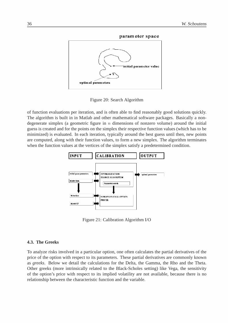
Figure 20: Search Algorithm
of function evaluations per iteration, and is often able to find reasonably good solutions quickly.The algorithm is built in in Matlab and other mathematical software packages. Basically a non-degenerate simplex (a geometric figure inn dimensions of nonzero volume) around the initialguess is created and for the points on the simplex their respective function values (which has to beminimized) is evaluated. In each iteration, typically around the best guess until then, new pointsare computed, along with their function values, to form a new simplex. The algorithm terminateswhen the function values at the vertices of the simplex satisfy a predetermined condition.
Figure 21: Calibration Algorithm I/O
4.3. The Greeks
To analyze risks involved in a particular option, one often calculates the partial derivatives of theprice of the option with respect to its parameters. These partial derivatives are commonly knownasgreeks. Below we detail the calculations for the Delta, the Gamma, the Rho and the Theta.Other greeks (more intrinsically related to the Black-Scholes setting) like Vega, the sensitivityof the option’s price with respect to its implied volatility are not available, because there is norelationship between the characteristic function and the variable.

The World of VG 37
4.3.1. DELTA
TheDelta of an option, often denoted by∆, measures the sensitivity of the option’s value to pricechanges in the underlying.
∆ =∂C(K, T )
∂S0.
In the Black-Scholes setting this Delta is giving the number of stocks one needs to hold in orderto perfectly hedge the option. In the more advanced models, perfect hedging is no longer alwayspossible and many other hedging strategies can be considered and maybe make more sense. Nev-ertheless, Delta-hedging is a very well-accepted strategy that is also straightforward to apply. Wemust note however that taking (partial) derivatives is a local operator, typically taking into accountcontinuous movements of the underlying. If we work with models in which the underlying priceprocess can jump, such a local operator does not tell the whole story.
We have :
∆ =∂
∂S0
[
exp(−α log(K))
π
∫ +∞
0
exp(−iv log(K))exp(−rT )φ(v − (α + 1)i; T )
α2 + α − v2 + i(2α + 1)vdv
]
=exp(−α log(K))
π
∫ +∞
0
exp(−iv log(K))exp(−rT )∂φ(v−(α+1)i ;T )
∂S0
α2 + α − v2 + i(2α + 1)vdv.
Now, assume the (risk-neutral) model for the price of the underlying at timeT is of the formST = S0ST , whereST is not depending onS0 anymore, thenlog(ST ) = log(S0) + log(ST ). Notethat this assumption is a very typical one and is the case for all models we consider. Furthermore,we have then that
∂φ(v − (α + 1)i; T )
∂S0
=∂
∂S0
E[exp(i(v − (α + 1)i)(log(S0) + log(ST ))]
=φ(v − (α + 1)i; T )(α + 1 + iv)
S0.
In conclusion
∆ =exp(−α log(K))
π
∫ +∞
0
exp(−iv log(K))exp(−rT )φ(v − (α + 1)i; T )(α + 1 + iv)
S0(α2 + α − v2 + i(2α + 1)v)dv;
=exp(−α log(K))
π
∫ +∞
0
exp(−iv log(K))exp(−rT )φ(v − (α + 1)i; T )
S0(α + iv)dv,
where we used in the last line the fact thatα2 + α − v2 + i(2α + 1)v = (α + iv)(α + 1 + iv).
4.3.2. GAMMA
TheGammaof an option, often denoted byΓ, measures the sensitivity of the Delta of the optionwith respect to price changes in the underlying.
Γ =∂∆
∂S0=
∂2C(K, T )
∂S20
.

38 W. Schoutens
High Gammas mean that the corresponding Delta-hedge position is very sensitive to changes inthe underlying price process.
Completely analogous as in the calculation of Delta, we have
Γ =exp(−α log(K))
π
∫ +∞
0
exp(−iv log(K))exp(−rT )∂2φ(v−(α+1)i ;T )
∂S20
α2 + α − v2 + i(2α + 1)vdv.
Under the same assumption on the form of the price process, we have then that
∂
∂S0
φ(v − (α + 1)i; T )
S0
=φ(v − (α + 1)i; T )(α + iv)
S20
.
Hence, in conclusion
Γ =exp(−α log(K))
π
∫ +∞
0
exp(−iv log(K))exp(−rT )φ(v − (α + 1)i; T )
S20
dv.
4.3.3. RHO
Rhoof an option, often denoted byρ (not to be confused with correlation later on), measures thesensitivity of the option’s value with respect to the risk free interest rater:
ρ =∂C(K, T )
∂r.
If we assume that the (risk-neutral) price of the underlying at timeT is of the formST =exp(rT )ST , whereST is not depending onr anymore, thenlog(ST ) = rT + log(ST ). Note thatthis assumption is again a very typical one. Calculations are performed in exactly the same was asabove; we find
ρ =exp(−α log(K))
π
∫ +∞
0
exp(−iv log(K))T exp(−rT )φ(v − (α + 1)i; T )
α + 1 + ivdv.
4.3.4. THETA
Also the value of Theta,Θ, i.e. the sensitivity of the option price with respect to the passage oftime can be calculated along the same lines. However, here the calculations dependent much moreon the explicit form of the characteristic function.
In general we have
Θ =∂
∂T
[
exp(−α log(K))
π
∫ +∞
0
exp(−iv log(K))exp(−rT )φ(v − (α + 1)i; T )
α2 + α − v2 + i(2α + 1)vdv
]
=exp(−α log(K))
π
∫ +∞
0
exp(−iv log(K))∂
∂T[exp(−rT )φ(v − (α + 1)i; T )]
α2 + α − v2 + i(2α + 1)vdv.
=exp(−α log(K) − rT )
π
∫ +∞
0
exp(−iv log(K))∂
∂Tφ(v − (α + 1)i; T ) − rφ(v − (α + 1)i; T )
α2 + α − v2 + i(2α + 1)vdv.

The World of VG 39
In case of the VG setting where
φV G(u; T ) = exp
(
iu log(S0) + T
(
iu(r − q + ω) + C log
(
GM
GM + (M − G)iu + u2
)))
,
we have that
∂
∂Tφ(u; T ) = φ(u; T )
(
iu(r − q + ω) + C log
(
GM
GM + (M − G)iu + u2
))
.
4.4. Calibration Results
Doing a global calibration for the VG model introduced in the previous Chapter, we obtain aserious improvement over the Black-Scholes case. However observe still a significant differencewith real market prices as can be seen in Figure 22. The initial parameters we started with where(C = 1, G = 5, M = 5); the final optimal parameters coming out of the calibration procedureare given by:(C = 1.3574, G = 5.8703, M = 14.2699)
1000 1100 1200 1300 1400 15000
20
40
60
80
100
120
140
160
180
SP−500 / 18−04−2002 / VG / ape = 4.67 %
strike
optio
n pr
ice
Figure 22: Global Calibration of VG
Fitting the smile at one maturity is done very accurately as can be seen in Figure 23. Theparameters coming out of the calibration procedure for each maturity are given in Table 7. We seea quite typical term-structure for theσ andν parameter.

40 W. Schoutens
1040 1060 1080 1100 1120 1140 1160 118010
20
30
40
50
60
70
80
90
Strike
Op
tio
n p
rice
SP500 / 18−04−2002 / VG (T=0.184) / ape =0.24034%
950 1000 1050 1100 1150 1200 12500
20
40
60
80
100
120
140
160
180
Strike
Op
tio
n p
rice
SP500 / 18−04−2002 / VG (T=0.436) / ape =0.21534%
950 1000 1050 1100 1150 1200 1250 13000
20
40
60
80
100
120
140
160
180
Strike
Op
tio
n p
rice
SP500 / 18−04−2002 / VG (T=0.692) / ape =0.34172%
1000 1050 1100 1150 1200 1250 1300 13500
50
100
150
Strike
Op
tio
n p
rice
SP500 / 18−04−2002 / VG (T=0.936) / ape =0.43269%
950 1000 1050 1100 1150 1200 1250 1300 1350 14000
20
40
60
80
100
120
140
160
180
200
Strike
Op
tio
n p
rice
SP500 / 18−04−2002 / VG (T=1.192) / ape =0.54975%
1050 1100 1150 1200 1250 1300 1350 1400 1450 15000
20
40
60
80
100
120
140
160
180
StrikeO
ptio
n p
rice
SP500 / 18−04−2002 / VG (T=1.708) / ape =0.48827%
Figure 23: Calibration of VG maturity per maturity
T σ ν θ0.184 0.1600 0.1141 -0.17880.436 0.1631 0.2702 -0.16390.692 0.1665 0.4888 -0.14590.936 0.1660 0.6263 -0.15451.192 0.1720 0.9109 -0.14851.708 0.1864 1.5414 -0.1396
Table 7: VG optimal parameters maturity per maturity
5. MONTE CARLO SIMULATION
Next, we look at possible simulation techniques for the processes encountered so far. A Levy pro-cess can be in general simulated based on a compound Poisson approximation. However, typically,for very specific processes like the VG other much faster techniques are available.
We assume we have random number generators at hand which can provide us Normal(0, 1) andGamma(a, b) random numbers. Throughoutvn always denotes a Normal(0, 1) random number;gn a Gamma random numbers.
A good reference book is [37].
5.1. Brownian Motion
Recall that a standard Brownian motionW = Wt, t ≥ 0 has Normal distributed independentincrements. We discretize time by taking time steps of size∆t, which we assume to be verysmall. We simulate (by the Euler scheme) the value of the Brownian motion at the time points

The World of VG 41
n∆t, n = 0, 1, . . .:W0 = 0, Wn∆t = W(n−1)∆t +
√∆tvn.
This leads to the following typical picture of standard Brownian motion
0 0.1 0.2 0.3 0.4 0.5 0.6 0.7 0.8 0.9 1−0.8
−0.6
−0.4
−0.2
0
0.2
0.4
0.6
0.8
1Standard Brownian Motion
Figure 24: A sample path of a standard Brownian motion
The Matlab code for this is very simple:T=1;N=250;dt=T/N;tt=[0:dt:T];
bm(1)=0;for j=2:N
bm(j)=bm(j-1)+sqrt(dt) * normrnd(0,1);
end;plot(tt, bm);
By making use of the powerful vector notation and operations one can replace the for-loop byjust a single line:T=1;N=250;dt=T/N;tt=[0:dt:T];bm=cumsum([0 sqrt(dt) * normrnd(0,1,1,N)]);plot(tt, bm);
5.2. The Gamma Process
Note that, whenX is Gamma(a, b), then forc > 0, X/c is Gamma(a, bc). So we need only a goodgenerator for Gamma(a, 1) random numbers. Most mathematical software programs have built in

42 W. Schoutens
random gamma number generators. In Matlab we have the commandgamrnd . Note Matlab usesanother convention for theb-parameter: one needs to invert theb-parameter of our setting.
To simulate a sample path of a Gamma processG = Gt, t ≥ 0, whereGt follows aGamma(at, b) law at time pointsn∆t, n = 0, 1, . . .:
• generate independent Gamma(a∆t, b) random numbersgn, n ≥ 1
• Then setG0 = 0 andGn∆t = G(n−1)∆t + gn, n ≥ 1.
The Matlab code for this is very simple:T=1;N=250;dt=T/N;tt=[0:dt:T];a=10; b=20;
gp(1)=0;for j=2:N
gp(j)=gp(j-1)+gamrnd(a * dt,1/b);
end;plot(tt, gp);
By making use of the powerful vector notation and operations one can one more replace thefor-loop by just a single line:T=1;N=250;dt=T/N;tt=[0:dt:T]gp=cumsum([0 gamrnd(a * dt,1/b,1,N)]);plot(tt,gp);
5.3. The Variance Gamma Process
5.3.1. VGAS THE DIFFERENCE OFTWO GAMMA PROCESSES
A VG process is the difference of two independent Gamma processes. More precisely a VGprocessX(V G) with parametersC, G, M > 0 can be decomposed as
X(V G)t = G
(1)t − G
(2)t ,
where

The World of VG 43
0 0.1 0.2 0.3 0.4 0.5 0.6 0.7 0.8 0.9 10
0.05
0.1
0.15
0.2
0.25
0.3
0.35Gamma Process (a=10; b=20)
Figure 25: A sample path of a Gamma process (a = 10 andb = 20.)
• G(1) is a Gamma process with parametersa = C andb = M ;
• G(2) is a Gamma process with parametersa = C andb = G.
0 0.1 0.2 0.3 0.4 0.5 0.6 0.7 0.8 0.9 1−0.15
−0.1
−0.05
0
0.05
0.1VG Process (C=20; G=40; M=50)
Figure 26: A sample path of a VG processC = 20, G = 40 andM = 50.
Matlab code for VG process as difference of two Gamma processes and the VG stock process:Snul=100; T=1; r=0.04; q=0.03; n=250;nu=0.2; sigma=0.15; theta= -0.10omega=log(1-sigmaˆ2 * nu/2-theta * nu)/nu;C=1/nu;G=(sqrt(thetaˆ2 * nuˆ2/4+sigmaˆ2 * nu/2)-theta * nu/2)ˆ(-1);M=(sqrt(thetaˆ2 * nuˆ2/4+sigmaˆ2 * nu/2)+theta * nu/2)ˆ(-1);
dt=T/n;tt=[0:dt:T];
S(1)=Snul;vg(1)=0;for s = 1:n

44 W. Schoutens
g1= gamrnd(dt * C,1/M);
g2= gamrnd(dt * C,1/G);
vg(s+1) = vg(s) + g1-g2;
S(s+1) = Snul * exp((r-q+omega) * tt(s+1)+vg(s+1));
end;Making use of vector notation, one could replace the lastfor -loop by
g1=[0,cumsum(gamrnd(dt * C,1/M,1,n))];g2=[0,cumsum(gamrnd(dt * C,1/G,1,n))];S = Snul * exp((r-q+omega) * tt+g1-g2);
5.3.2. VGAS TIME-CHANGED BROWNIAN MOTION
A VG processX(V G) with parameters(σ, ν, θ) out of a standard Brownian motionW with drift bya Gamma processG with parametersa = 1/ν andb = 1/ν. We have
X(V G)t = θGt + σWGt
.
VG(σ, ν, θ)-random numbershn can be obtained out of Gamma(ν−1, ν−1) random numbersgn
and Normal(0, 1) numbersvn:hn = θgn + σ
√gnvn.
Matlab code for VG process as Gamma-time-changed Brownian Motion with drift:Snul=100; T=1; r=0.04; q=0.03; n=250;nu=0.2; sigma=0.15; theta= -0.10omega=log(1-sigmaˆ2 * nu/2-theta * nu)/nu;
dt=T/n;tt=[0:dt:T];
vg(1)=0;for s = 1:n
g= gamrnd(dt/nu,nu);
vg(s+1) = vg(s) + theta * g+ sigma * sqrt(g) * normrnd(0,1);
end;S = Snul * exp((r-q+omega). * tt+vg);

The World of VG 45
6. APPENDIX: CHARACTERISTIC FUNCTIONS
In this appendix we given more details about characteristic functions, essential mathematical ob-jects in the financial engineering.
Characteristic functions provide us a way to describe the dynamics/stochastics of some popularadvanced models unambiguously. Moreover, out of them one can obtain many interesting proper-ties of the underlying distribution like moments. Finally and maybe for us most importantly, theyserve as main input in our vanilla pricing algorithm which will be constructed in Section 4.
The characteristic functionφ of a distribution, or equivalently of a random variableX, is theFourier-Stieltjes transform of the distribution functionF (x) = P (X ≤ x):
φX(u) = E[exp(iuX)] =
∫ +∞
−∞
exp(iux)dF (x),
where i is the imaginary number (i2 = −1).
In almost all cases we will work with a random variableX that has a continuous distributionwhich has a density function, sayfX(x). One then can write:
φX(u) = E[exp(iuX)] =
∫ +∞
−∞
exp(iux)fX(x)dx.
Example: The Normal Distribution Normal(µ, σ2), with meanµ and varianceσ2 lives on(−∞, +∞)and has a density function given by:
f(x; µ, σ2) =1√
2πσ2exp
(
−(x − µ)2
2σ2
)
Its characteristic function is given by
φX(u) =
∫ +∞
−∞
exp(iux)1√
2πσ2exp
(
−(x − µ)2
2σ2
)
dx
= exp(iuµ) exp
(
−1
2σ2u2
)
.
Let us prove the above formula for the Normal(0, 1) case. We will comment later on how to
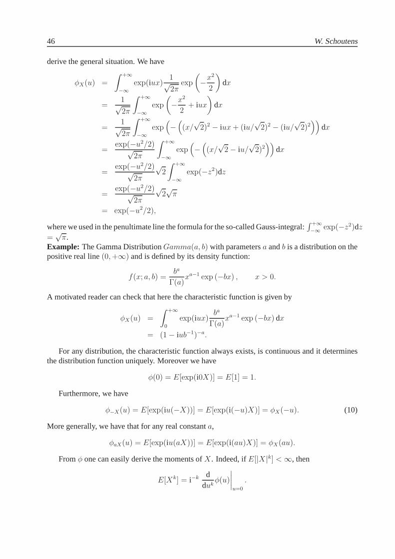
46 W. Schoutens
derive the general situation. We have
φX(u) =
∫ +∞
−∞
exp(iux)1√2π
exp
(
−x2
2
)
dx
=1√2π
∫ +∞
−∞
exp
(
−x2
2+ iux
)
dx
=1√2π
∫ +∞
−∞
exp(
−(
(x/√
2)2 − iux + (iu/√
2)2 − (iu/√
2)2))
dx
=exp(−u2/2)√
2π
∫ +∞
−∞
exp(
−(
(x/√
2 − iu/√
2)2))
dx
=exp(−u2/2)√
2π
√2
∫ +∞
−∞
exp(−z2)dz
=exp(−u2/2)√
2π
√2√
π
= exp(−u2/2),
where we used in the penultimate line the formula for the so-called Gauss-integral:∫ +∞
−∞exp(−z2)dz
=√
π.Example: The Gamma DistributionGamma(a, b) with parametersa andb is a distribution on thepositive real line(0, +∞) and is defined by its density function:
f(x; a, b) =ba
Γ(a)xa−1 exp (−bx) , x > 0.
A motivated reader can check that here the characteristic function is given by
φX(u) =
∫ +∞
0
exp(iux)ba
Γ(a)xa−1 exp (−bx) dx
= (1 − iub−1)−a.
For any distribution, the characteristic function always exists, is continuous and it determinesthe distribution function uniquely. Moreover we have
φ(0) = E[exp(i0X)] = E[1] = 1.
Furthermore, we have
φ−X(u) = E[exp(iu(−X))] = E[exp(i(−u)X)] = φX(−u). (10)
More generally, we have that for any real constanta,
φaX(u) = E[exp(iu(aX))] = E[exp(i(au)X)] = φX(au).
Fromφ one can easily derive the moments ofX. Indeed, ifE[|X|k] < ∞, then
E[Xk] = i−k dduk
φ(u)
∣
∣
∣
∣
u=0
.

The World of VG 47
A very convenient property, is the fact that the sum of two independent random variable, orequivalently the convolution of two distributions, translate into the product of the correspondingcharacteristic functions. More precisely, ifX andY are two independent random variables withcharacteristic functionsφX andφY resp., then the characteristic function ofZ = X + Y is givenby
φZ(u) = φX(u)φY (u). (11)
Next, note that the degenerate random variableX ≡ µ, i.e. the random variable that takes withprobability one the constant valueµ (so there is no randomness), has characteristic function
E[exp(iuX)] = exp(iuµ).
Example: Using the above properties, we can easily deduce the characteristic function of a randomvariableZ with the Normal(µ, σ2) distribution. Indeed, writeZ = µ + σX with X standardNormal. Then
φZ(u) = φµ+σX(u)
= φµ(u)φσX(u)
= φµ(u)φX(σu)
= exp(iuµ) exp(−(σu)2/2)
References
[1] Abramowitz, M. and Stegun, I.A. (1968)Handbook of Mathematical Functions. Dover Publ.,New York.
[2] Artzner, P., Delbaen, F., Eber, J.-M. and Heath, D. (1999) Coherent measures of risk.Math.Finance9(3), 203–228.
[3] Asmussen, S. and Rosinski, J. (2001) Approximations of small jumps of Levy processes witha view towards simulation.J. Appl. Probab.38 (2), 482–493.
[4] Artzner, P. and Heath, D. (1995) Approximate completeness with multiple martingale mea-sures.Math. Finance5, 1–11.
[5] Bachelier, L. (1900) Theorie de la speculation.Ann. Sci. Ecole. Norm. Sup.17, 21–86.
[6] Bar-Lev, S., Bshouty, D. and Letac, G. (1992) Natural exponential families and self-decomposability.Statistics and Probability Letters13, 147–152.
[7] Barndorff-Nielsen, O.E. (1977) Exponentially decreasing distributions for the logarithm ofparticle size.Proceedings of the Royal Society London A353, 401–419.
[8] Barndorff-Nielsen, O.E. (1978) Hyperbolic distributions and distributions on hyperbolae.Scandinavian Journal of Statistics5, 151–157.

48 W. Schoutens
[9] Barndorff-Nielsen, O.E. (1995)Normal inverse Gaussian distributions and the modeling ofstock returns. Research Report No. 300, Department of Theoretical Statistics, Aarhus Uni-versity.
[10] Barndorff-Nielsen, O.E. (1996) Normal Inverse Gaussian distributions and stochastic volatil-ity models.Scandinavian Journal of Statistics24, 1–13.
[11] Barndorff-Nielsen, O.E. (1998) Processes of normal inverse Gaussian type.Finance andStochastics2, 41–68.
[12] Barndorff-Nielsen, O.E. and Halgreen, C. (1977) Infinitely divisibility of the hyperbolicand generalized inverse Gaussian distributions.Zeitschrift fur Wahrscheinlichkeitstheorie undverwandte Gebiete38, 309–311.
[13] Barndorff-Nielsen, O.E., Mikosch, T. and Resnick, S. (Eds.) (2001)Levy Processes - Theoryand Applications.Boston: Birkhauser.
[14] Barndorff-Nielsen, O.E. and Shephard, N. (2001) Modelling by Levy Processes for FinancialEconometrics. In: O.E. Barndorff-Nielsen, T. Mikosch and S. Resnick (Eds.):Levy Processes- Theory and Applications, Birkhauser, Boston, 283–318.
[15] Barndorff-Nielsen, O.E. and Shephard, N. (2001) Non-Gaussian Ornstein-Uhlenbeck-basedmodels and some of their uses in financial economics.Journal of the Royal Statistical Society,Series B63, 167–241.
[16] Barndorff-Nielsen, O.E. and Shephard, N. (2001)Integrated OU processes and non-GaussianOU-based stochastic volatility models., working paper.
[17] Barndorff-Nielsen, O.E., Nicolata, E. and Shephard, N. (2002) Some recent developments instochastic volatility modelling.Quantitative Finance2, 11–23.
[18] Bakshi, G. and Madan, D.B. (2000) Spanning and derivative security valuation.FinancialEconomics55, 205–238.
[19] Beirlant, J., Goegebeur, Y., Segers, J., and Teugels, J. (2004)Statistics of Extremes: Theoryand Applications. Wiley.
[20] Blæsild, P. (1978)The Shape of the Generalized Inverse Gaussian and Hyperbolic Distribu-tions. Research Report No. 37, Department of Theoretical Statistics, Aarhus University.
[21] Berman, M.B. (1971)Generating gamma distributed variates for computer simulation mod-els. Technical Report R-641-PR, Rand Corporation.
[22] Bertoin, J. (1996)Levy Processes. Cambridge Tracts in Mathematics121, Cambridge Uni-versity Press, Cambridge.
[23] Biane, P., Pitman J. and Yor, M. (2001) Probability laws related to the Jacobi theta and Rie-mann zeta functions, and Brownian excursions.Bull. Amer. Math. Soc.38, 435–465.

The World of VG 49
[24] Bingham, N.H. and Kiesel, R. (1998)Risk-Neutral Valuation. Pricing and Hedging of Finan-cial Derivatives. Springer Finance, London.
[25] Black, F. and Scholes, M. (1973) The pricing of options and corporate liabilities.Journal ofPolitical Economy81, 637–654.
[26] Broadie, M., Glasserman, P. and and Kou, S.G. (1997) A continuity correction for discretebarrier options.Math. Finance7 (4), 325–349.
[27] Broadie, M., Glasserman, P. and and Kou, S.G. (1999) Connecting discrete and continuouspath-dependent options.Finance and Stochastics2, 1–28.
[28] Carr, P. and Madan, D. (1998) Option Valuation using the Fast Fourier Transform.Journal ofComputational Finance2, 61–73.
[29] Carr, P., Geman, H., Madan, D.H. and Yor, M. (2000) The fine structure of asset returns: anempirical investigation.Journal of Business, to appear.
[30] Carr, P., Geman, H., Madan, D.H. and Yor, M. (2001)Stochastic Volatility for Levy Processes.Prebluciations du Laboratoire de Probabilites et Modeles Aleatoires645, Universites de Paris6 & Paris 7, Paris.
[31] Chan, T. (1999) Pricing contingent claims on stocks driven by Levy processes.Annals ofApplied Probability9, 504–528.
[32] Clark, P. (1973) A subordinated stochastic process model with finite variance for speculativeprices.Econometrica41, 135–156.
[33] Cont, R. (2001) Empirical properties of asset returns: stylized facts and statistical issues.Quantitative Finance1, 223–236.
[34] Cox, J., Ingersoll, J. and Ross, S. (1985) A theory of the term structure of interest rates.Econometrica53, 385–408.
[35] Delbaen, F. (2000)Coherent Risk Measures on General Probability Spaces.ETHZ Preprint,Zurich.
[36] Delbaen, F. and Schachermayer, W. (1994) A general version of the fundamental theorem ofasset pricing.Math. Ann.300, 463–520.
[37] Devroye, L. (1986)Non-Uniform Random Variate Generation. Springer-Verlag, New York.
[38] Dritschel,M. and Protter, P. (1999) Complete Markets with discountinuous security price.Finance and Stochastics3, 203–214.
[39] Eberlein, E. and Jacod, J. (1997) On the range of options prices.Finance and Stochastics1(2), 131–140.
[40] Eberlein, E. and Keller, U. (1995) Hyperbolic distributions in finance.Bernoulli1, 281–299.

50 W. Schoutens
[41] Eberlein, E., Keller, U. and Prause, K. (1998) New insights into smile, mispricing and valueat risk: The hyperbolic model.Journal of Business71 (3), 371–406.
[42] Eberlein, E. and Prause, K. (1998)The Generalized Hyperbolic Model: Financial Derivativesand Risk Measures.FDM preprint 56. University of Freiburg.
[43] Eberlein, E. and Raible, S. (1999) Term structure models driven by general Levy processes.Mathematical Finance9 (1), 31–53.
[44] Elliot, R.J. and Kopp, P.E.(1999)Mathematics of Financial MarketsSpringer. New York.
[45] Engel, D. (1982)The Multiple Stochastic IntegralMem. Amer. Math. Soc.38 (265).
[46] Fama, E. (1965): The Behaviour of Stock Market Prices.Journal of Business, Vol. 38, pp.34-105
[47] Fisher, R.A. and Tippett, L.H.C. (1928) On the estimation of the frequency distributions ofthe largest or smallest member of a sample.Proceedings of the Cambridge PhilosophicalSociety24, 180–190.
[48] Gnedenko, B.V. (1943) Sur la distribution limite du terme maximum d’une serie aleatoire.Annals of Mathematics44, 423–453.
[49] Geman, H., Madan, D. and Yor, M. (2001) Time changes for Levy Processes.MathematicalFinance11, 79–96.
[50] Gerber, H.U. and Shiu, E.S.W. (1994) Option pricing by Esscher-transforms.Transactions ofthe Society of Actuaries46, 99–191.
[51] Gerber, H.U. and Shiu, E.S.W. (1996) Actuarial bridges to dynamic hedging and option pric-ing. Insur. Math. Econ.18 (3), 183–218.
[52] Good, I.J. (1953) The population frequencies of species and the estimation of populationparameters.Biometrika40, 237–260.
[53] Grigelionis, B. (1999) Processes of Meixner Type.Lith. Math. J.39 (1), 33–41.
[54] Grigelionis, B. (2000)Generalizedz-Distributions and related Stochastic Processes. Matem-atikos Ir Informatikos Institutas Preprintas Nr. 2000-22, Vilnius.
[55] Gumbel, E.J. (1958)Statistics of Extremes. Columbia University Press.
[56] Halgreen, C. (1979) Self-decomposability of the generalized inverse Gaussian and hyperbolicdistributions.Zeitschrift fur Wahrscheinlichkeitstheorie und verwandte Gebiete47, 13–18.
[57] Harrison, J.M. and Kreps, D.M. (1979) Martingales and arbitrage in multiperiod securitiesmarkets.J. Econom. Theory20, 381–408.
[58] Harrison, J.M. and Pliska, S.R. (1981) Martingales and stochastic integrals in the theory ofcontinuous trading.Stochastic Processes Appl.11, 215–260.

The World of VG 51
[59] Heston, S.L. (1993) A closed form solution for options with stochastic volatility with appli-cations to bonds and currency options.Review of Financial Studies6(2), 327–343.
[60] Hudson, R.L. and Mandelbrot, Benoit B. (2004)The (Mis)Behavior of Markets – A FractalView of Risk, Ruin and Reward.Perseus Books Group.
[61] Hull, J.C. and White, A. (1988) The pricing of Options on Assets with Stochastic Volatility.Journal of Finance42, 281–300.
[62] Hull, J.C. (2000)Options, Futures and Other Derivatives(4th edition). Prentice-Hall.
[63] Hunt, P.J. and Kennedy, J.E. (2000)Financial Derivatives in Theory and Practice. Wiley,Chichester.
[64] Ito, K. (1951) Multiple Wiener integral.J. Mathematical Society of Japan3 (1), 157–169.
[65] Jarrow, R.A., Jin, X. and Madan, D.B. (1999) The second fundamental theorem of assetpricing.Math. Finance9, 255–273.
[66] Johnk, M.D. (1964) Erzeugung von Betaverteilten und Gammaverteilten Zufallszahlen.Metrika 8, 5–15.
[67] Jørgensen, B. (1982)Statistical Properties of the Generalized Inverse Gaussian Distribution.Lecture notes in Statistics9, Springer-Verlag, New York.
[68] Jyrek, Z.J. and Vervaat, W. (1983) An integral representation for selfdecomposable Banachspace valued random variables.Zeitschrift fur Wahrscheinlichkeitstheorie und verwandte Ge-biete62, 247–262.
[69] Karatzas, I. and Shreve S.E. (1996)Brownian Motion and Stochastic Calculus(2nd edition).Springer, New York.
[70] Kloeden, P.E. and Platen, E. (1992)Numerical Solutions of Stochastical Differential Equa-tions. Springer, Berlin.
[71] Koekoek, R. and Swarttouw, R.F. (1998)The Askey-scheme of hypergeometric orthogonalpolynomials and itsq-analogue.Report 98-17, Delft University of Technology.
[72] Kreps, D. (1981) Arbitrage and equilibrium in economics with infinitely many commodities.Journal of Mathematical Economics8, 15–35.
[73] Levy, P. (1937)Theories de L’Addition Aleatories. Gauthier-Villars, Paris.
[74] Lukacs, E. (1970)Characteristic Functions.Griffin. London.
[75] Madan, D.B., Carr, P. and Chang, E.C. (1998) The variance gamma process and option pric-ing. European Finance Review2, 79–105.
[76] Madan, D.B. and Milne, F. (1991) Option pricing with V.G. martingale components.Mathe-matical Finance1(4), 39–55.

52 W. Schoutens
[77] Madan, D.B. and Seneta, E. (1987) Chebyshev polynomial approximations and characteristicfunction estimation.Journal of the Royal Statistical Society Series B49(2), 163–169.
[78] Madan, D.B. and Seneta, E. (1990) The v.g. model for share market returns.Journal of Busi-ness63, 511–524.
[79] Mandelbrot, Benoit B. (1962) The variation of certain speculative prices.IBM Research Re-port NC-87.
[80] Mandelbrot, Benoit B. (1962b) Sur certains prix speculatifs: faits empiriques et modele basesur les processus stables additifs de Paul Levy.Comptes rendus (Paris)254, 3968–3970.
[81] Mandelbrot, Benoit B. (1963) The variation of certain speculative prices.Journal of Business36, 394–419.
[82] Mandelbrot, Benoit B. (1967) The variation of some other speculative prices.Journal ofBusiness40, 393–413.
[83] Mandelbrot, Benoit B. and Taylor, H.M. (1967) On the distribution of stock price differences.Operations Research15, 1057–1062.
[84] Marcus, A.H. (1975) Power laws in compartmental analysis. Part I: a unified stochasticmodel.Math. Biosci.23, 337–350.
[85] Marcus, M.B. (1987)ζ-Radial Processes and Random Fourier Series, Memoirs of the Amer-ican Mathematical Society368.
[86] Merton, R.C. (1973) Theory of rational option pricing.Bell J. Econom. Managem. Sci.4,141–183.
[87] Michael, J.R., Schucany, W.R., and Haas, R.W. (1976) Generating random variates usingtransformations with multiple roots.The American Statistician30, 88-90.
[88] Nicolata, E. and Venardos, E. (2000) Derivative pricing in Barndorff-Nielsen and Shephard’sOU type stochastic volatility models. Unpublished paper: Dept. of Mathematical Sciences,Aarhus University.
[89] Nualart, D. and Schoutens W. (2000) Chaotic and predictable representations for Levy pro-cesses.Stochastic Processes and their Applications90 (1), 109–122.
[90] Nualart, D. and Schoutens W. (2001) Backwards Stochastic Differential Equations andFeynman-Kac Formula for Levy Processes, with applications in finance.Bernoulli7(5), 761–776.
[91] Pickands III, J. (1975) Statistical inference using extreme order statistics.Annals of Statistics3, 119–131.
[92] Pitman, J. and Yor, M. (2000)Infinitely divisible laws associated with hyperbolic functions.Prebluciations du Laboratoire de Probabilites et Modeles Aleatoires616, Universites de Paris6 & Paris 7, Paris.

The World of VG 53
[93] Pollard, D. (1984)Convergence of stochastic processes. Springer Series in Statistics.Springer-Verlag, New York.
[94] Prause, K. (1999)The Generalized Hyperbolic Model: Estimation, Financial Derivatives,and Risk Measures. Ph.D. thesis, Freiburg i. Br.
[95] Protter, Ph. (1990)Stochastic Integration and Differential Equations. Springer-Verlag. Berlin.
[96] Protter, Ph. (2001) A partial introduction to financial asset pricing theory.Stochastic Pro-cesses and their Applications91, 169–203.
[97] Raible, S. (2000)Levy Processes in Finance: Theory, Numerics, and Empirical Facts.Ph.D.thesis, Freiburg i. Br.
[98] Rosinski, J. (1991) On a class of infinitely divisible processes represented as mixtures ofGaussian processes. In: Cambanis, S., Samorodnitsky, G. and Taqqu, M.S. (Eds.)StableProcesses and Related Topics. Birkhauser, Basel, 27–41.
[99] Rosinski, J. (2000) Series representations of Levy processes from the perspective of pointprocesses. In: O.E. Barndorff-Nielsen, T. Mikosch and S. Resnick (Eds.):Levy Processes -Theory and Applications, Birkhauser, Boston, 283–318.
[100] Rydberg, T. (1996)The Normal Inverse Gaussian Levy Process: Simulations and Approxi-mation. Research Report 344, Dept. Theor. Statistics, Aarhus University.
[101] Rydberg, T. (1996)Generalized Hyperbolic Diffusions with Applications Towards Finance.Research Report 342, Dept. Theor. Statistics, Aarhus University.
[102] Rydberg, T. (1997) A note on the existence of unique equivalent martingale measures in aMarkovian setting.Finance and Stochastics1, 251–257.
[103] Rydberg, T. (1998)Some Modelling Results in the Area of Interplay between Statistics,Mathematical Finance, Insurance and Econometrics. PhD thesis, University of Aarhus.
[104] Samuelson, P. (1965) Rational theory of warrant pricing.Industrial Management Review6,13–32.
[105] Sato, K. (2000)Levy Processes and Infinitely Divisible Distributions. Cambridge Studies inAdvanced Mathematics 68. Cambridge University Press, Cambridge.
[106] Sato, K., and Yamazato, M. (1982) Stationary processes of Ornstein-Uhlenbeck type. In: K.Ito and J.V. Prohorov (Eds.),Probability Theory and Mathematical Statistics, Lecture Notesin Mathematics1021. Springer, Berlin.
[107] Sato, K., Watanabe, T. and Yamazato, M. (1994) Recurrence conditions for multidimen-sional processes of Ornstein-Uhlenbeck type.J. Math. Soc. Japan46, 245–265.
[108] Sato, K. (1999)Levy Processes and Infinitely Divisible Distributions. Cambridge Studies inAdvanced Mathematics bf 68. Cambridge University Press, Cambridge.

54 W. Schoutens
[109] Schoutens, W. and Teugels, J.L. (1998) Levy processes, polynomials and martingales.Com-mun. Statist.- Stochastic Models14 (1 and 2), 335–349.
[110] Schoutens, W. (2000)Stochastic Processes and Orthogonal Polynomials. Lecture Notes inStatistics 146. Springer-Verlag, New York.
[111] Schoutens, W. (2001)The Meixner Process in Finance.EURANDOM Report 2001-002,EURANDOM, Eindhoven.
[112] Schoutens, W. (2002)Meixner Processes: Theory and Applications in Finance.EURAN-DOM Report 2002-004, EURANDOM, Eindhoven.
[113] Schoutens, W. (2003)Levy Processes in Finance: Pricing Financial Derivatives. Wiley.
[114] Schoutens, W. and Cariboni, J (2009)Levy Processes in Credit Risk. Wiley.
[115] Schoutens, W. and Studer, M. (2001)Stochastic Taylor Expansions for Poisson Processesand Applications towards Risk Management.EURANDOM Report 2001-005, EURAN-DOM, Eindhoven.
[116] Shaw, W.T. (1998)Modelling financial derivatives with Mathematica.Cambridge Univer-sity Press.
[117] Sichel, H.S. (1974) On a distribution representing sentence-length in written prose.J. R.Statist. Soc. A137, 25–34.
[118] Sichel, H.S. (1975) On a distribution law for word frequencies.J. Amer. Statist. Soc Ass.70,542–547.
[119] Tompkins, R. and Hubalek, F. (2000) On closed form solutions for pricing options withjumping volatility. Unpublished paper: Technical University, Vienna.
[120] Tweedie, M.C.K (1947) Functions of a statistical variate with given means, with specialreference to Laplacian distributions.Proceedings of the Cambridge Philosophical Society43, 41–49.
[121] Wald (1947)Sequential Analysis. Wiley, New York.
[122] Wise, M.G. (1975) Skew distributions in biomedicine including some with negative powersof time. In: Statistical Distributions in Scientific Work, Vol. 2: Model building and Modelselection (G.P. Patil et al., eds.), Dordrect Reidel, 241–262.
[123] Wolfe, S.J. (1982) On a continuous analogue of the stochastic difference equationρXn+1 +Bn. Stoch. Prob. Appl.12, 301–312.
[124] Yor, M. (1992)Some Aspects of Brownian Motion, Part I: Some Special Functionals. Lec-tures in Mathematics ETH Zurich, Birkhauser Verlag, Berlin.

CONTRIBUTED TALKS
55

56

DEATH BONDS WITH STOCHASTIC FORCE OF MORTALITY
Francesco Menoncin
Department of Economics, Brescia University, Via S. Faustino, 74/B, 25122 Brescia, ItalyEmail: [email protected]
Abstract
In a financial market with stochastic interest rate following a square root process, we presenta closed form solution for pricing a death bond (as a security backed by insurance contracts)when the force of mortality follows a square root stochastic process whose expected valuecoincides, at any time, with the force of mortality given by the so-called Gompertz Makehamdensity.
1. INTRODUCTION AND CONCLUSION
The managers of either an insurance company or a pension fund are concerned about both financialand actuarial risks. Nevertheless, these two kinds of risk can be partially or fully hedged withvery different instruments. For instance, the inflation risk, the interest rate risk, and the exchangerate risk, can all be efficiently hedged by existing financial assets (respectively, inflation indexedbonds, floating coupon bonds, and forwards, futures, or options on the foreign exchange). For whatconcerns the actuarial risk, its hedging and diversification are more difficult because of the lackof traded assets which could be able to provide their holder with cash flows correlated with theabove mentioned risks. Furthermore, since the financial assets are usually very poorly (when notat all) correlated with the actuarial risk sources, then there is no portfolio of financial asset that canprovide a suitable hedging against the actuarial risk. Accordingly, in order to be able to effectivelyhedge against actuarial risk, the institutional investors should trade, on the financial market, newassets correlated with death (or survival) probability of economic agents. Such assets wouldn’tof course provide any hedging against the so-called basis risk, i.e. the risk that the population anactuarial-financial asset is written on diverges from the population whose demographic behaviourwe are trying to hedge against. Nevertheless, these actuarial-financial assets would make manyinstitutional investors able to bear the so-called longevity and mortality risks. The longevity riskcould be almost perfectly hedged through longevity bonds (see, for instance, Azzoppardi 2005,Menoncin 2006, 2008) and, in the same spirit, there are nowadays rumors about the issue of somenew assets called death bonds which should belong to the family of the Asset Backed Securities
57
58 F. Menoncin
(ABS). In particular, death bonds should be backed by death insurance sold by their holder inexchange of the net present value of the final benefit. One of the main concern about both longevityand mortality risk is that the force of mortality (given by the amount of people who die in agiven period as a percentage of the whole population) is stochastic itself. In fact, once it hasbeen estimated and foreseen on the basis of the actuarial tables, it is nevertheless affected byunforeseeable factors. In particular, the length of human life (for both men and women) has beensignificantly increasing during the last decades. Such an increase implies a serious risk for pensionfunds which will have to pay pensions for periods longer than that they had foreseen when enteringthe pension agreements with their sponsors. The force of mortality (or the survival probability) canbe profitably modelling by using well known results about stochastic processes (see, for instance,Dahl 2004, Biffis 2005, Hainaut and Devolder 2008). In this paper we present a model for thestochastic force of mortality following a generalized Cox et al. (1985) process and consistent withthe so-called Gompertz Makeham density function (see, for instance, Milevsky 2006). In thisframework, we are able to price a death insurance/death bond in a closed form and we show thatthe return on a death bond is decreasing through time. The rest of the paper is structured as follows.Section 2 shows the model for the instantaneously riskless interest rate and a zero-coupon bondwritten as a derivative on the interest rate. Section 3 presents the model we take into accountfor the stochastic force of mortality. Section 4 and 5 contain the main result about pricing a deathinsurance and a death bond both in a stochastic framework. Section 6 concludes. The technicalitiesabout the main results are left to appendices.
2. INTEREST RATE AND BONDS
The instantaneously riskless interest rate r(t) is assumed to follow the stochastic differential equa-tion (Cox et al. 1985)
dr(t) = ar (γr − r(t)) dt+ σr√r(t) dWr(t), (1)
r (t0) = r0,
with positive constant r0 and where Wr(t) is a Brownian motion. For pricing purposes, we need tocompute the stochastic process (1) under a risk-neutral probability measure (Q). After Girsanov’stheorem we know that on an arbitrage free financial market there exists (at least) a market price ofrisk ξr such that
dWQr = ξrdt+ dWr.
Here, we assume that the market price of risk is given by ξr =√r(t) ψ
σr, with ψ constant so
that the process of r(t) under Q can be written in the same form as (1):
dr(t) = aQr
(γQr − r(t)
)dt+ σr
√r(t) dWQ
r , (2)
withaQr ≡ ar + ψ, γQ
r ≡ar
ar + ψγr.
In this framework, we can state what follows.

Death bonds with stochastic force of mortality 59
Proposition 2.1 If the riskless interest rate follows (1), then the price of a zero-coupon B(t, T ) isgiven by
B(t, T ) = EQt
[e−
∫ Tt r(s)ds
]= e−a
Qr γ
Qr
∫ Tt CB(s,T )ds−CB(t,T )r(t), (3)
where
CB(t, T ) = 21− e−k(T−t)
k + aQr +
(k − aQ
r
)e−k(T−t)
, (4)
k ≡√(
aQr
)2+ 2σ2
r
whose differential is
dB(t, T )
B(t, T )= r(t)dt− CB(t, T )σr
√r(t) dWQ
r (t) (5)
=(r(t)− CB(t, T )σr
√r(t)ξr
)dt− CB(t, T )σr
√r(t) dWr(t).
Proof. See Appendix A with X = r and B(t, T ) = V (t, T )|χ=0.Another way to write the value of a zero-coupon is to use the forward (instantaneous) interest
rate f (t, T ):B(t, T ) = e−
∫ Tt f(t,s)ds,
where we do not need any longer the expected value since the whole curve of the forward ratef(t, s) is known in t for any s ≥ t.
An obvious no-arbitrage condition asks for the expected discounted value of r(T ) to equate theexpected discounted value of f(t, T ):
EQt
[r(T )e−
∫ Tt r(s)ds
]= EQ
t
[f(t, T )e−
∫ Tt r(s)ds
],
but since f(t, T ) belongs to the information set (i.e. σ−algebra) in t, then we have
f(t, T ) =EQt
[r(T )e−
∫ Tt r(s)ds
]EQt
[e−
∫ Tt r(s)ds
] .
Proposition 2.2 If the riskless interest rate r(t) follows the process (1), then the forward interestrate is given by
f(t, T ) =
∫ T
t
aQr γ
Qr e−
∫ Ts (aQ
r+CB(u,T )σ2r)duds+ e−
∫ Tt (aQ
r+CB(u,T )σ2r)dur(t), (6)
where CB(t, T ) is as in (4), and whose differential is
df(t, T ) = e−∫ Tt (aQ
r+CB(u,T )σ2r)duCB(t, T )σ2
rr(t)dt
+e−∫ Tt (aQ
r+CB(u,T )σ2r)duσr
√r(t) dWQ
r ,
where it is true that∂CB(t, T )
∂T= e−
∫ Tt (aQ
r+CB(u,T )σ2r)du.
Proof. See Appendix A with X = r and f(t, T ) =V (t,T )|χ=1
V (t,T )|χ=0.
We will show these results have a straight parallel in an actuarial framework.
60 F. Menoncin
3. MORTALITY RATE
Let us call τ the (stochastic) death time whose density function is π (τ). In this way the probabilityof surviving from t0 up to t, for an agent aged t0, is given by
(tpt0) = 1−∫ t
t0
π(s)ds,
whose differential isd (tpt0)
(tpt0)= − π(t)
1−∫ tt0π(s)ds
dt ≡ −λ(t)dt, (7)
with the natural boundary condition (t0pt0) = 1. In the actuarial literature, λ(t) is often calledmortality rate (or hazard rate). The (unique) solution of the ordinary differential equation (7) is
(tpt0) = e−
∫ tt0λ(s)ds
. (8)
One of the most common parametrizations for the mortality rate is the so called Gompertz-Makeham function:
λ(t) = φ+1
bet−mb , (9)
where the positive constant have the following meaning: (i) φ captures the age independent com-ponent of mortality rate (like accidents), (ii) m measures the modal value of life, and (iii) b isthe dispersion parameter of life. Typical value for these parameters (consistently chosen withMilevsky, 2006) are
φ = 0.001, m = 82.3, b = 11.4. (10)
In the real world the mortality rate does not behave in a deterministic way. In fact, it maychange for unforeseeable reasons. In order to fix that, we can model λ(t) as a stochastic processitself:
dλ(t) = µλ(t, λ)dt+ σλ(t, λ)dW (t),
λ(t0) = λ0.
In this case the survival probability cannot be written as in (8). In fact, under the informationset in t, we do not know all the mortality rates from t to T . Accordingly, we can compute thesurvival probability from t0 to t only under the expected value conditional to the information setin t0:
(tpt0) = Et0
[e−
∫ tt0λ(s)ds
]. (11)
We highlight that, in this case, the expected value is computed under the historical probabilitymeasure (we haven’t put any upper script on the expected value), and not under the risk neutralprobability.
If we are allowed to differentiate with respect to time (t) under the expected value1, then wecan conclude from (7) that
π(t) = −d (tpt0)
dt= Et0
[λ(t)e
−∫ tt0λ(s)ds
].
1Grandell (1976) shows that the equality which follows is true if: (i) there exists a constant C such that, for any t,Et0[λ(t)2
]< C, and (ii) for any ε > 0 and almost every time t, limδ→0 P (|λ (t+ δ)− λ(t)| ≥ ε) = 0.
Death bonds with stochastic force of mortality 61
In this case the hazard rate is given by
l(t0, t) ≡ −d (tpt0)
dt
1
(tpt0)=
Et0
[λ(t)e
−∫ tt0λ(s)ds
]Et0
[e−
∫ tt0λ(s)ds
] , (12)
which coincides with λ(t) if and only if λ(t) is not stochastic (of course it is true, in any case, thatl (t0, t0) = λ(t0)).
Such a framework has a straightforward and appealing parallel with the financial framework wehave already presented above. The main difference is that the expected value on the financial mar-ket is computed under the riskless probability measure (Q) which is different from the probabilitymeasure used for computing (tpt0) (see table 1).
Actuarial market Financial marketDeath intensity λ(t) Interest rate r(t)
Survival probability (tpt0) Zero-coupon bond price B(t0, t)Hazard rate l(t0, t) Instant forward rate f(t0, t)
Computations under P Computations under Q
Table 1: Correspondences between actuarial and financial frameworks
Now, we want to build a stochastic process for the variable λ(t) such that its expected valueis, at any instant, equal to the Gompertz-Makeham mortality rate (9). For this purpose, we use thefollowing result.
Proposition 3.1 If the stochastic variable X(t) solves
dX(t) = α(t)
(1
α(t)
∂β(t)
∂t+ β(t)−X(t)
)dt+ σ(t,X)dW (t),
X(t0) = β(t0),
thenEt0 [X(t)] = β(t).
Proof. Let us apply Ito’s lemma to Y (t) = X(t)e∫ tt0α(u)du:
dY (t) = e∫ tt0α(u)du
dX(t) + α(t)X(t)e∫ tt0α(u)du
dt
=∂
∂t
(β(t)e
∫ tt0α(u)du
)dt+ e
∫ tt0α(u)du
σ(t,X)dW (t).
Now, we compute the expected value under the information set in t0:
Et0 [dY (t)] =∂
∂t
(β(t)e
∫ tt0α(u)du
)dt,
and by integrating from t0 up to t we have
Et0 [Y (t)] = Y (t0) + β(t)e∫ tt0α(u)du − β(t0).
62 F. Menoncin
After substituting for Y we finally obtain
Et0 [X(t)] = (X(t0)− β(t0)) e−
∫ tt0α(u)du
+ β(t),
and, since X(t0) = β(t0), the result of the proposition is obtained.We want the expected value of λ(t) to be always equal to the Gompertz function (9), i.e.
Et0 [λ(t)] = φ+1
bet−mb . (13)
By using the result of Proposition 3.1, we can write the process for λ(t) as
dλ(t) = aλ (γλ(t)− λ(t)) dt+ σλ√λ(t) dWλ(t), (14)
λ(t0) = φ+1
bet0−mb ,
where
γλ(t) ≡ φ+
(1
aλb+ 1
)1
bet−mb , (15)
and aλ and σλ are two constant (and positive) parameters that can be estimated from the historicalseries on λ(t).
In order to trace our model back to the well known results about the affine stochastic processes,we have chosen to set the diffusion term as the square root of the stochastic variable λ(t) itself.
Since we need the force of mortality to be always positive, we give now a condition underwhich λ(t) never becomes negative.
Proposition 3.2 If
σ2λ ≤ 2aλ
(φ+
(1
aλb+ 1
)1
bet0−mb
),
then the value of λ(t) in (14) never becomes negative.
Proof. See Appendix B.
Proposition 3.3 If the death intensity λ(t) follows the process (14), then the survival probabilityis given by
(Tpt) = e−aλ∫ Tt CP (s,T )γλ(s)ds−CP (t,T )λ(t), (16)
where
CP (t, T ) = 21− e−k(T−t)
k + aλ + (k − aλ) e−k(T−t), (17)
k ≡√a2λ + 2σ2
λ,
and, in differential terms,
d (Tpt)
(Tpt)= λ(t)dt− CP (t, T )σλ
√λ(t) dWλ(t).

Death bonds with stochastic force of mortality 63
Proof. See Appendix A.
Proposition 3.4 If the death intensity λ(t) follows the process (14), then the hazard rate is givenby
l(t, T ) =
∫ T
t
aλγλ(s)e−
∫ Ts (aλ+CP (u,T )σ2
λ)duds+ e−∫ Tt (aλ+CP (u,T )σ2
λ)duλ(t), (18)
whose differential is
dl(t, T ) = e−∫ Tt (aλ+CP (u,T )σ2
λ)duCP (t, T )σ2λλ(t)dt (19)
+e−∫ Tt (aλ+CP (u,T )σ2
λ)duσλ√λ(t) dWλ(t),
where the function CP (t, T ) is as in (17).
Proof. See Appendix A.
4. DEATH INSURANCE
The subscriber of a death insurance agrees to pay settlements (P ) during his lifetime in order toreceive, at his death, a given amount of money (final benefit). For the sake of simplicity we willset such an amount to 1
If the death insurance is subscribed in t0 (i.e. when the subscriber is aged t0), then the actuarialequilibrium for such a contract asks for the expected present value of the settlements to equate theexpected present value of the final benefit (available at the death time τ and equal to 1). If weassume that P is continuously paid, then the actuarial equilibrium asks for the following equalityto hold:
Eτt0
[∫ τ
t0
P (s)e−
∫ st0rλ(u)du
ds
]= Eτ
t0
[e−
∫ τt0rλ(u)du
],
where rλ is a suitable discount rate used by the insurance company.When the insurance contract enters (in any way) the financial market, then the value of the
contract must be computed as the value of any other asset i.e. under the risk neutral probabilitymeasure. Accordingly, the discount rate rλ is replaced by the riskless interest rate r as follows
EQ,τt0
[∫ τ
t0
P (s)e−
∫ st0r(u)du
ds
]= EQ,τ
t0
[e−
∫ τt0r(u)du
].
Now, as it is usually the case, the riskless interest rate r is assumed to be independent ofthe death time τ . Accordingly, the expected value computed under Q and τ can be separatelycomputed, and the equilibrium condition becomes∫ ∞
t0
EQ,τt0 [Is<τ ] EQ
t0
[P (s)e
−∫ st0r(u)du
]ds =
∫ ∞t0
EQ,τt0 [π(s)] EQ
t0
[e−
∫ st0r(u)du
]ds

64 F. Menoncin
where Iε is the indicator function whose value is 1 if the event ε happens and 0 otherwise. Sincethe expected value of the indicator function coincides with the probability of ε then we have∫ ∞
t0
EQt0
[e−
∫ st0λ(u)du
]EQt0
[P (s)e
−∫ st0r(u)du
]ds
=
∫ ∞t0
EQt0
[λ(s)e
−∫ st0λ(u)du
]EQt0
[e−
∫ st0r(u)du
]ds,
and, if P is constant we have
P ∗ =
∫∞t0
EQt0
[λ(s)e
−∫ st0λ(u)du
]B(t0, s)ds∫∞
t0EQt0
[e−
∫ st0λ(u)du
]B(t0, s)ds
.
By recalling (12) and (11),we can finally write
P ∗ =
∫∞t0l(t0, t)
Q (tpt0)QB(t0, s)ds∫∞
t0(tpt0)
QB(t0, s)ds, (20)
where we have indicated with (tpt0)Q and l (t0, t)
Q the survival probability and the hazard raterespectively, computed under the risk neutral probability.
Once the value of the premium is obtained, the value of the death insurance, at any time t, isgiven by the difference between the expected present value of the final benefit and the expectedpresent value of the premia still due:
D(t) = EQ,τt
[e−
∫ τt r(u)du
]− P ∗EQ,τ
t
[∫ τ
t
e−∫ st r(u)duds
],
which can be simplified as we have done above by obtaining
D(t) =
∫ ∞t
(l(t, s)Q − P ∗
)(spt)
QB(t, s)ds. (21)
As it is evident from this last equation, the value of the premium for a death insurance sub-scribed in t0 can also be computed from (21) by imposing the condition D(t0) = 0.
From Equation (21) it is evident that the death insurance cannot be distinguished from aninfinitely living bond whose coupons are given by the difference between the hazard rate and theequilibrium premium, weighted by the survival probability.
The differential form of (21) is
dD(t)
D(t)=
(r(t) + λ(t) +
P ∗ − λ(t)
D(t)
)dt (22)
+Dr(t)
D(t)σr√r dWQ
r +Dλ(t)
D(t)σλ√λ dWQ
λ ,
where Dλ and Dr are the partial derivatives of D with respect to λ and r respectively and, inparticular,
∂D(t)
∂λ(t)=
∫ ∞t
e−∫ st (aλ+CP (u,s)σ2
λ)du (spt)QB(t, s)ds
−∫ ∞t
CP (t, s)(l(t, s)Q − P ∗
)(spt)
QB(t, s)ds,

Death bonds with stochastic force of mortality 65
The seller
Insurancecompany
Buyer
Hedge fundInvestment bank
Investors
-
?
Premia
6Premia
6
-Insurance
NPV
?
Finalbenefit
1
2
3
2
-Insurance
NPV 3Premia
+Final
benefit
3
?
Coupons
Deathbond4
Finalbenefit
Life settlementbroker
Life settlementprovider
Figure 1: How a death insurance becomes a death bond
∂D(t)
∂r(t)= −
∫ ∞t
CB (t, s)(l (t, s)Q − P ∗
)(spt)
QB(t, s)ds.
5. DEATH BOND
A death bond belongs to the family of the Asset Backed Security (ABS). The process for changinga death insurance into a death bond is made by 4 steps (as in figure 1). Let us see such steps indetails.
1. The so-called seller is the subscriber of the death insurance. When the agent becomes older(typically 70) and he does not have any further need for the insurance on his life, he wouldlike to cash out his policy.
2. The seller hires a life settlement broker who will find a buyer for his policy who pays the netpresent value of the policy (we have called D(t) in the previous section). Thus, the buyerwill continue paying the settlements to the insurance company and he will also receive thefinal benefit when the seller dies. The up-front payout to the seller varies widely, from 20%of the death benefit to 40%. The seller pays to the broker a commission ranged from 5% to6%.
3. Another character in this game is the so-called life settlement provider. Through him, a hedgefund or an investment bank buys a pool of death insurances from insurance companies. Now,the hedge fund will receive the premia from the buyer and will pay the final benefit.
4. In the last step, after a sufficient number of policies has been collected, these policies canback the emission of a death bond. Accordingly, the policies play the same role as the

66 F. Menoncin
Figure 2: Return on a death bond (dDD
) with t0 = 25 and r = 0.05 for t going from 30 to 110.
assets in an ABS or the mortgages in a mortgage backed security. The new death bond is apass through asset: the premia received by the hedge fund are directly paid to the investors(without any guarantee provided by the hedge fund).
From Equation (22) we can see that the return on a death bond is given by r(t)+λ(t)+ P ∗−λ(t)D(t)
.In a fully deterministic case with the values of the parameters given in (10), r = 0.05, and t0 = 25,the premium is given by P ∗ = 0.0066 and the return on the death bond for time t going from 30 to110 is plotted in figure 2.
It is evident that the bond return decreases while time goes on. In fact, the best case for thebuyer of the death bond is when the seller immediately dies after receiving the first premium P ∗.
A. COMPUTATION OF Et
[(1− χ+ χX(t)) e−
∫ Tt X(s)ds
]If the stochastic variable X(t) follows the process
dX(t) = a (γ(t))−X(t)) dt+ σ√X(t) dW (t), (23)
X (t0) = X0,
then the expected value
V (t, T ) = Et
[(1− χ+ χX(T )) e−
∫ Tt X(s)ds
],
must solve the partial differential equation
∂V
∂t+∂V
∂Xa (γ(t)−X) +
1
2
∂2V
∂X2σ2X = XV,

Death bonds with stochastic force of mortality 67
with the boundary conditionV (T, T ) = 1− χ+ χX(T ),
where the parameter χ can take either value 1 or value 0. If χ = 0, then the function V coincideswith the probability (Tpt) if X = λ and with the value of a zero-coupon if X = r. Instead, ifχ = 1, then the function V coincides with the numerator of l (t, T ) in Equation (12).
Now we use the guess function
V (t,X) = (E(t) + F (t)X) e−A(t)−C(t)X ,
where the function A, C, E, and F must be computed in order to solve the previous differentialequation. The boundary condition translates into the following conditions:
E(T ) = 1− χ, F (T ) = χ, A(T ) = 0, C(T ) = 0.
Once the partial derivatives of V are substituted into the differential equation we obtain asecond order polynomial in X . Since we want it to be identically zero, then the coefficients of itsterms must be zero. This means that we can split the differential equation into three differentialequations as follows2
0 =
∂E
∂t+ Faγ(t)− E (At + Caγ(t)) ,
0 =∂F
∂t− F (At + Caγ(t))− Fa− CFσ2,
0 = −∂C∂t
+ aC + 12C2σ2 − 1.
(24)
We immediately see that the value of function C(t) can be computed from the third equation.With the suitable boundary condition the only solution of the differential equation for C(t) is givenby
C (t, T ) = 21− e−k(T−t)
k + a+ (k − a)e−k(T−t),
k ≡√a2 + 2σ2.
The values of all the other functions can be written as functions of C(t, T ). Now, if we wantedto compute just the survival probability, then we would have E = 1 and F = 0 with the functionA accordingly solving
0 =∂A
∂t+ Caγ(t),
with the boundary condition A(T ) = 0. The only solution of this equation is
A(t) = a
∫ T
t
C(s)γ(s)ds.
2For the sake of simplicity, we have omitted the functional dependences (except for the function γ(t)).

68 F. Menoncin
Given this value for A(t), the two first equations of system (24) become
0 =∂E(t)
∂t+ F (t)aγ(t),
0 =∂F (t)
∂t− F (t)
(a+ C(t)σ2
).
We now compute the value of F from the second equation by obtaining
F (t) = χe−∫ Tt (a+C(s)σ2)ds,
and the value of E can then be computed from the first equation
E(t) = 1− χ+ a
∫ T
t
F (s)γ(s)ds.
Finally, we can write
V (t, T ) =
(1− χ+ χ
∫ T
t
aγ(s)e−∫ Ts (a+C(u)σ2)duds+ χe−
∫ Tt (a+C(u)σ2)duX(t)
)×e−a
∫ Tt C(u)γ(u)du−C(t)X(t).
The two values we are interested into are given by
V (t, T )|χ=0 = e−a∫ Tt C(u)γ(u)ds−C(t)X(t),
andV (t, T )|χ=1
V (t, T )|χ=0
=
∫ T
t
aγ(s)e−∫ Ts (a+C(u)σ2)duds+ e−
∫ Tt (a+C(u)σ2)duX(t).
B. PROOF OF PROPOSITION 3.2
If X(t) follows (23) with γ(t)) constant, then it is well known that X(t) never becomes negativeif σ2 ≤ 2aγ. In order to prove the proposition, we use the following result.
Proposition B.1 Let us assume we have two continuous, adapted processes Xi(t), i = 1, 2, suchthat
Xi(t) = Xi(t0) +
∫ t
t0
µi (s,Xi(s)) ds+
∫ t
t0
σ (s,Xi(s)) dW (s),
and ∀t ∈ [t0,∞[ , x ∈ R, y ∈ R: (i) the coefficients µi(t, x) and σ(t, x) are continuous, real-valued functions, (ii) |σ(t, x)− σ(t, y)| ≤ h (|x− y|) where h : [0,∞[ × [0,∞[ is a strictly in-creasing function with h(0) = 0 and
∫(0,ε)
h−2(u)du = ∞, ∀ε > 0, (iii) X1(t0) ≤ X2(t0) a.s.,(iv) µ1(t, x) ≤ µ2(t, x), (v) there exists a positive constant K such that either µ1(t, x) or µ2(t, x)satisfies |µi(t, x)− µi(t, y)| ≤ K |x− y|. Then
P X1(t) ≤ X2(t), ∀t ∈ [t0,∞[ = 1.
Death bonds with stochastic force of mortality 69
Proof. See Karatzas and Shreve (1991), Proposition 2.18 p. 293.Here, we take the following process
λ1(t) =
(φ+
1
bet0−mb
)+
∫ t
t0
a (γ(t0)− λ1(s)) ds+
∫ t
t0
σ√λ1(s) dW (s),
λ2(t) =
(φ+
1
bet0−mb
)+
∫ t
t0
a (γ(s)− λ2(s)) ds+
∫ t
t0
σ√λ2(s) dW (s),
where γ(t) is defined in (15). It is evident that both the drift and the diffusion terms respect all theconditions in Proposition B.1.
Since we have set λ1(t0) = λ2(t0) and we know that λ1(t) never becomes negative if
σ2 ≤ 2aγ(t0), (25)
then we also know that λ2(t) never becomes negative if its drift is greater than λ1(t)’s:
a (γ(t)− λ(t)) ≥ a (γ(t0)− λ(t)) ,
for any real λ and for any t ∈ [t0,∞[. Such inequality holds if and only if γ(t) ≥ γ(t0). Neverthe-less, since γ(t) is strictly increasing in t, then this inequality always holds. This means that λ2(t)never becomes negative if just (25) holds.
References
M. Azzoppardi. The longevity bond. In First International Conference on Longevity Risk andCapital Markets Solutions, London, UK, 2005.
E. Biffis. Affine processes for dynamic mortality and actuarial valuations. Insurance: Mathematicsand Economics, 37:443–468, 2005.
J.C. Cox, J.E. Jr. Ingersoll, and S.A. Ross. A theory of the term structure of interest rates. Econo-metrica, 53:385–407, 1985.
M. Dahl. Stochastic mortality in life insurance: market reserves and mortality-linked insurancecontracts. Insurance: Mathematics and Economics, 35:113–136, 2004.
D. Hainaut and P. Devolder. Mortality modelling with Levy processes. Insurance: Mathematicsand Economics, 42:409–418, 2008.
I. Karatzas and S.E. Shreve. Brownian Motion and Stochastic Calculus. Springer, 1991.
F. Menoncin. Understanding longevity bonds. Life and Pensions, November 2006.
F. Menoncin. The role of longevity bonds in optimal portfolios. Insurance: Mathematics andEconomics, 42:343–358, 2008.
M. Milevsky. The Calculus of Retirement Income. Cambridge, 2006.

70 F. Menoncin
GENERIC PRICING OF FX, INFLATION AND STOCK OPTIONS UNDERSTOCHASTIC INTEREST RATES AND STOCHASTIC VOLATILITY
Alexander van Haastrecht†§ and Antoon Pelsser†
† Netspar/University of Amsterdam, Dept. of Quantitative Economics, Roetersstraat 11, 1018 WBAmsterdam, The Netherlands§Delta Lloyd Insurance, Risk Management, Spaklerweg 4, PO Box 1000, 1000 BA AmsterdamEmail: [email protected], [email protected]
Abstract
We consider the pricing of FX, inflation and stock options under stochastic interest rates andstochastic volatility, for which we use a generic multi-currency framework. We allow for ageneral correlation structure between the drivers of the volatility, the inflation index, the do-mestic (nominal) and the foreign (real) rates. Having the flexibility to correlate the underlyingFX/Inflation/Stock index with both stochastic volatility and stochastic interest rates yields arealistic model, which is of practical importance for the pricing and hedging of options withlong-term exposures. We derive explicit pricing formulas for various securities, such as vanillacall options, forward starting options, inflation-indexed swaps and inflation caps. We considera calibration example to FX market data and finally we conclude.
1. INTRODUCTION
The markets for long maturity and hybrid derivatives are developing more and more. Not onlyare increasingly exotic structures created, also the markets for plain vanilla derivatives are grow-ing. One of the recent advances is the development of long maturity option markets across variousasset classes. During the last years, long maturity securities, such as Target Auto RedemptionNotes (TARN) equity-interest rate options (e.g. see Caps (2007)), Power-Reverse Dual-Currency(PRDC) Foreign Exchange (FX) swaps (e.g. see Piterbarg (2005)) and inflation-indexed LimitedPrice Indices (LPI) structures (e.g see Brigo and Mercurio (2006)) have become increasingly pop-ular. Whereas for FX, inflation and hybrid structures –which explicitly depend on future interestrates evolutions– it is immediately clear that the use of stochastic interest rates is crucial in aderivative pricing model, the addition of stochastic rates is also important for the pricing and inparticularly the hedging of long maturity equity derivatives (e.g. see Bakshi et al. (2000)).
Most investment banks have now standardized a three-factor modeling framework to pricecross-currency (i.e., FX and inflation) options (e.g. see Sippel and Ohkoshi (2002) or Jarrow and
71

72 A. van Haastrecht and A.A.J. Pelsser
Yildirim (2003)). The index then follows a log-normal process, and the interest rates of bothcurrencies are driven by one-factor Gaussian models (e.g. see Hull and White (1993)). The choiceof Gaussian assumptions for the interest rates and the log-normality for the index has allowedfor a very efficient, essentially closed-form, calibration to at-the-money options on the index, i.e.,on the FX-rate or stock price. The assumption of log-normality for an index, though technicallyvery convenient, does not find a justification in the financial equity markets (e.g. see Bakshi et al.(1997)), nor in the FX markets (e.g. see Piterbarg (2005)) nor in the inflation markets (e.g. seeMercurio and Moreni (2006)). In fact, the markets for these products exhibit a strong volatilityskew or smile, implying log index returns deviating from normality and suggesting the use ofskewed and heavier tailed distributions. Moreover, many multi-currency structures (like LPIs orPRDCs) are particularly sensitive to volatility skews/smiles as they often incorporate multiplestrikes as well as callable/knockout components.
Hence, appropriate exotic option pricing models, which need to quantify the volatility expo-sure in such structures, should at least be able to incorporate the smiles/skews in the vanilla mar-kets. While various methods exist to incorporate volatility smiles (i.e., local volatility, stochasticvolatility and/or jumps), the calibration of such models is by no means trivial. Normally, a skew-mechanism is applied to the forward index price (i.e., the FX-rate, CPI/Equity index), however,to price multi-currency options also a term-structure involving various time points of the forwardindex is required. The incorporation of stochastic interest rates makes the connection between thetwo particularly non-trivial (e.g. see Piterbarg (2005) or Antonov et al. (2008)). Though the issueis important, Piterbarg (2005) even dubs it as ‘perhaps even the most important current outstand-ing problems for quantitative research departments worldwide’, there is remarkably little literatureavailable on the subject even though the problem attracted both the attention of practitioners aswell as from academia (e.g. see van der Ploeg (2007)).
Only very recently, a few approaches were suggested. A local volatility approach is used inPiterbarg (2005), who derives approximating formulas for calibration. Andreasen (2006) combinesHeston (1993) stochastic volatility with independent stochastic interest rates drivers and derivesclosed-form Fourier expressions for vanilla options. To correlate the independent rate drivers withthe FX-rate, Andreasen (2006) uses an indirect approach in the form of a volatility displacementparameter, which has some disadvantages as that it can lead to extreme model parameters (e.g. seeAntonov et al. (2008)). The calibration of FX options’ stochastic interest rates with Heston (1993)stochastic volatility under a full correlation structure is undertaken in Antonov et al. (2008) whouse Markovian projection to derive approximation formulas. Though their projection techniqueis elegant, the quality of their approximation deteriorates for larger maturities or more extrememodel parameters. The exact pricing of FX options under Schobel and Zhu (1999) stochasticvolatility, single-factor Gaussian rates and a full correlation structure was recently considered invan Haastrecht et al. (2008).
In this paper, building on the results of van Haastrecht et al. (2008), Andreasen (2006) andPiterbarg (2005), we consider the pricing of foreign exchange, inflation and stock options underSchobel and Zhu (1999) and Heston (1993) stochastic volatility and under multi-factor Gaussianinterest rates with a full correlation structure. Since stock and FX options are special (nested) casesof inflation-indexed caps/floors1, we will mainly focus on the pricing of inflation index derivatives.
1In our framework an inflation option can be seen as forward-starting FX-option, hence the pricing of FX-optionfollows from the pricing of inflation option by setting the forward starting date equal to the current date. A stock
Generic pricing of FX, inflation and stock options 73
The stock and FX model option pricing formulas hence follow directly from our generalization ofthe foreign exchange inflation framework of Jarrow and Yildirim (2003).
The setup of the paper is as follows. In Section 2, we introduce our new model. The cor-responding pricing methodology is considered in Section 3.1, while in Section 3.2 we derive thecharacteristic functions required for the Fourier-based pricing methods under Schobel and Zhu(1999) stochastic volatility, and touch upon the case with Heston (1993) stochastic volatility2.Section 4 considers a calibration example to FX market data, and finally Section 5 concludes.
2. MODELING FRAMEWORK
Before introducing the general model, we first recall the Jarrow and Yildirim (2003) model whichcan be seen as a special (degenerate) case of our model. The Jarrow and Yildirim (2003) frameworkfor modeling inflation and real rates is based on a foreign-exchange analogy between the real of andthe nominal economy. That is, the real rates are seen as interest rates in the real (foreign) economy,whereas the nominal rates represent the interest rates in the nominal (domestic) economy. Theinflation index then represents the exchange rate between the nominal (domestic) and real (foreign)currency.
The general model can be seen as an extension of the models of Jarrow and Yildirim (2003),see also van Haastrecht et al. (2008). That is, instead of one-factor Hull and White (1993) modelsfor the instantaneous nominal and real rates, we let the short rate be driven by multiple (correlated)factors. To ease the notation, we use an equivalent additive formulation for Hull-White interestrates in terms of a sum of correlated Gaussian factors plus a deterministic function, i.e., we writethe model into an affine factors formulation, cf Duffie et al. (2000, 2003). The deterministic factorcan be chosen as to exactly fit the term structure of the nominal or real interest rates, e.g. see Brigoand Mercurio (2006) or Pelsser (2000). If the nominal short interest rate is driven by K correlatedGaussian factors and the real short rate by M factors, the multi-factor Gaussian interest can berepresented as:
n(t) = ϕn(t) +K∑i=1
xin(t), r(t) = ϕr(t) +M∑j=1
xjr(t), (1)
where ϕn(t), ϕr(t) are the deterministic functions to fit the nominal and real term structure (inparticular ϕn(0) = n(0) and ϕr(0) = r(0)) and with xin(t), xjr(t) the Gaussian factors which driverespectively the nominal and real rates.
The second extension included in our model is that we make the volatility σI stochastic. More-over, we allow this stochastic volatility factor, which we denote by ν(t) from now on, to be corre-lated with the instantaneous interest rates and the inflation index. Two popular choices within thestochastic volatility literature are the models of Heston (1993) and Schobel and Zhu (1999). In the
option can be seen as an FX-option in which (possibly deterministic) foreign interest rates represent the continuousdividend yield.
2We refer the reader to van Haastrecht and Pelsser (2008) for more extensive pricing results under Heston (1993)stochastic volatility.

74 A. van Haastrecht and A.A.J. Pelsser
latter the volatility is modeled as an Ornstein-Uhlenbeck process
dν(t) = κ[ψ − ν(t)
]dt+ τdWν(t), ν(0) = ν0 (2)
with κ, ψ, σν positive parameters and where Wν(t) is a Brownian motion that is correlated with theother driving factors, especially the asset price. Note that we have a positive probability that ν(t)in (2) can become negative, which will cause the correlation between ν(t) and the other drivingfactors to (temporarily) change sign.
The most popular stochastic volatility model, however, is the Heston (1993) model, whichmainly owns its popularity due to its analytical tractability. In the Heston model, the variance ismodeled by the following Feller/CIR/square-root process
dν2(t) = κ[θ − ν2(t)
]dt+ ξν(t)dWν(t), ν2(0) = ν2
0 (3)
with κ, θ, ξ positive parameters and where Wν represents again a Brownian motion that is corre-lated with the other model factors.
With the multi-factor Gaussian rates and with stochastic volatility like Schobel-Zhu or Heston,we come to the following proposition for the dynamics of our model.
Proposition 2.1 TheQn dynamics of theK-factor instantaneous nominal rate n(t),M -factor realrate r(t) and the inflation index I(t), are given by
dxin(t) = −ainxin(t)dt+ σindWni(t), i = 1, . . . , K, (4)
dxjr(t) =[−ajrxjr(t)− ρI,xj
rν(t)σjr
]dt+ σjrdWrj (t), j = 1, . . . ,M, (5)
dI(t) = I(t)[n(t)− r(t)
]dt+ ν(t)I(t)dWI(t), (6)
with ain, ajr, σ
in, σ
jr positive parameters, ν(t) the stochastic volatility factor with dynamics given by
(2) or (3), and where (Wn1 , . . . ,WnK,Wr1 , . . . ,WrM ,Wν) is a Brownian motion under Qn with
(possibly) a full correlation structure.
The multi-factor Gaussian model is still very tractable, e.g. one has analytical formulas for theprices of a zero-coupon bond.
3. PRICING AND APPLICATIONS
In this section, we will briefly discuss the main vanilla inflation, FX and equity derivatives, anddiscuss how these securities can be priced in a closed-form by our model. Before turning to themarket-specific structures, we first consider the general pricing methodology.
3.1. Pricing
We will now discuss the general option pricing framework for inflation, FX and stock options.That is, we briefly review the framework of Carr and Madan (1999) for the pricing of European

Generic pricing of FX, inflation and stock options 75
options using Fourier inversion. Afterwards, we show how this framework can be applied to valueinflation, FX and stock derivatives. Under the risk-neutral measure Q (i.e., with the bank accountas numeraire), we can write the following expression for the price CT (k) of an European option(ω = 1 for a call, ω = −1 for a put) maturing at time T , with strike K = exp(k), on an asset I:
CT (k, ω) = IEn
e−
∫ Tit n(u)du
[ω(I(T )−K
)]+∣∣Ft. (7)
Hence, note that in order to price European options, we only need the probability distribution of theT -forward stock price at time T . Therefore, instead of evaluating expected discounted payoff underthe risk-neutral bank account measure, we can also change the underlying probability measureto evaluate this expectation under the T -forward probability measure QT (e.g. see Geman et al.(1996)). This is equivalent to choosing the T -discount bond as numeraire. Hence, conditional ontime t, we can evaluate the price of a European option (ω = 1 for a call, ω = −1 for a put) withstrike K = exp(k) as
CT (k, ω) = Pn(t, T )IEQT
n
[ω
(ITF (T )−K
)]+∣∣Ft (8)
where Pn(t, T ) denotes the price of a (pure) discount bond and ITF (t) := I(t)Pn(t,T )
denotes the T -forward index price. The above expression can be numerically evaluated by means of a Fourierinversion of the log-asset price characteristic function; following Carr and Madan (1999), Lewis(2001) and Lord and Kahl (2007), we can then write the call option price (7) with log strike k,in terms of the (T -forward) characteristic function φT of the T -forward log index price z(T ) :=log ITF (t). Provided that the regularity conditions for the Fourier Transformations are satisfied, i.e.,α > 0 for a call (ω = 1) and α > 1 for a put (ω = −1), one can write the following for thecorresponding European option price:
CT (k, ω, α) =Pn(t, T )
π
∞∫0
Re(e−(α+iv)kψT (v, ω, α)
)dv, (9)
with
ψT (v, ω, α) :=φT
(v − (ωα + 1)i
)(ωα + iv)(ωα + 1 + iv)
, (10)
and where φT (u) := IEQT
[exp(iuz(T )
)∣∣Ft] denotes the T -forward characteristic function of the
log index price. Note that (9) can be efficiently evaluated, i.e., either by direct integration or byFast Fourier Transformation, see Carr and Madan (1999), Lee (2004) or Lord and Kahl (2007).Thus, for the pricing of call and put options on some underlying asset, it suffices to know thecharacteristic function of the underlying. In the following sections, we derive the characteristicfunctions under Schobel and Zhu (1999) stochastic volatility, whereas the case with Heston (1993)stochastic volatility is discussed in van Haastrecht and Pelsser (2008).

76 A. van Haastrecht and A.A.J. Pelsser
3.2. Schobel-Zhu stochastic volatility
In this section we will determine the characteristic function (under the T -forward measure) of theforward log-inflation return y(Ti−1, Ti) between times Ti−1 and Ti. Therefore, we first need to de-termine the characteristic function of the T -forward log-inflation rate zT for a general maturity T .Building on the results of van Haastrecht et al. (2008), where the characteristic function is derivedfor the one-factor Schobel-Zhu-Hull-White model, we will derive its multi-factor generalization inthe following subsection.
3.2.1. CHARACTERISTIC FUNCTION OF THE LOG-INDEX PRICE
Using a partial differential approach, we will now determine the characteristic function of the logindex price of the dynamics (Proposition 2.1) with Schobel and Zhu (1999) stochastic volatility.First, recall that z(t) := log IF (t) is defined as the T -forward log-asset price; subject to the ter-minal boundary condition f(T, z, ν) = exp
(iuz(T )
), the Feynman-Kac theorem implies that the
expected value of exp(iuz(T )
), equals the solution of the Kolmogorov backward partial differen-
tial equation for the joint probability distribution function f(t, z, ν), i.e.
f := f(t, z, ν) = IEQT[exp(iuz(T )
)∣∣Ft]. (11)
Thus, the solution for f equals the characteristic function of the forward asset price dynamics(starting from z at time t). To obtain the Kolmogorov backward partial differential equation for thejoint probability distribution function f = f(t, y, ν), we need to take into account the covarianceterm dz(t)dν(t) which equals
dz(t)dν(t) =(ρIντν(t) +
K∑i=1
ρxinντσinB
in(t, T )−
K∑j=1
ρxjrντσjrB
jr(t, T )
)dt. (12)
The model we are considering is not an affine model in z(t) and ν(t), but it will be one if weenlarge the state space and include ν2(t):
dz(t) = −1
2ν2F (t)dt+ νF (t)dW T
F (t), (13)
dν(t) = κ[ξ(t)− ν(t)
]dt+ τdW T
ν (t), (14)
dν2(t) = 2ν(t)dν(t) + τ 2dt = 2κ( τ 2
2κ+ ξ(t)ν(t)− ν2(t)
)dt+ 2τν(t)dWν(t). (15)
Using (13) and (12), we obtain the following partial differential equation for f(t, z, ν):
0 = ft −1
2ν2F (t)fz + κ
(ξ(t)− ν(t)
)fν +
1
2ν2F (t)fzz
+(ρIντν(t) +
K∑i=1
ρxinντσinB
in(t, T )−
M∑j=1
ρxjrντσjBj
r(t, T ))fzν +
1
2τ 2fνν . (16)

Generic pricing of FX, inflation and stock options 77
Solving this partial differential equation, provides us with the characteristic function of the forwardasset price dynamics (starting from z at time t). Due to the affine structure of our model, we cometo the following proposition.
Proposition 3.1 The characteristic function of domestic T -forward log inflation-rate of the modelwith Schobel and Zhu (1999) stochastic volatility is given by the following closed-form solution:
f(t, z, ν) = exp[A(u, t, T ) +B(u, t, T )z(t) + C(u, t, T )ν(t) +
1
2D(u, t, T )ν2(t)
], (17)
where:
A(u, t, T ) = −1
2u(i+ u)VK,M(t, T )
+
T∫t
[κψ + (iu− 1)
K∑i=1
ρxinντσinB
in(t, T )− iu
M∑j=1
ρxjrντσjrB
jr(t, T )
]C(u, s, T )
+1
2τ 2(C2(u, s, T ) +D(u, s, T )
)ds,
B(u, t, T ) = B := iu,
C(u, t, T ) = −u(i+ u
)γ1 + γ2e−2γ(T−t)
γ0
(1 + e−2γ(T−t)
)+
K∑i=1
[(γi3 − γi4e−2γ(T−t)
)−(γi5e−ai
n(T−t) − γi6e−(2γ+ain)(T−t)
)− γi7e−γ(T−t)
]−
M∑j=1
[(γj8 − γ
j9e−2γ(T−t)
)−(γj10e
−ajr(T−t) − γj11e
−(2γ+ajr)(T−t)
)− γj12e
−γ(T−t)]
D(u, t, T ) = −u(i+ u
) 1− e−2γ(T−t)
γ1 + γ2e−2γ(T−t) .
Here, VK,M(t, T ) represents the integrated variance of the Gaussian rate processes (e.g. see vanHaastrecht and Pelsser (2008)), and
γ =√
(κ− ρIντB)2 − τ 2(B2 −B), γ0 =κψ
γ
γ1 = γ + (κ− ρI,ντB), γ2 = γ − (κ− ρI,ντB),
γi3 =ρI,xi
nσinγ1 + ρxi
nνσinτ(iu− 1)
ainγ, γi4 =
ρI,xinσinγ2 − ρxi
nνσinτ(iu− 1)
ainγ,
γi5 =ρI,xi
nσinγ1 + ρxi
n,νσinτ(iu− 1)
ain(γ − ain), γi6 =
ρI,xinσinγ2 − ρxi
n,νσinτ(iu− 1)
ain(γ + ain),
γj8 =ρI,xj
rσjrγ1 + ρxj
r,νσjrτB
ajrγ, γj9 =
ρI,xjrσjrγ2 − ρxj
r,νσjrτB
ajrγ,
γj10 =ρI,xj
rσjrγ1 + ρxj
r,νσjrτB
ajr(γ − ajr), γ11 =
ρI,xjrσjrγ2 − ρxj
r,νσjrτB
ajr(γ + ajr),
γi7 = (γi3 − γi4)− (γi5 − γi6), γj12 = (γj8 − γj9)− (γj10 − γ
j11).

78 A. van Haastrecht and A.A.J. Pelsser
Proof. See van Haastrecht and Pelsser (2008).
3.2.2. CHARACTERISTIC FUNCTION OF LOG INDEX RETURN
Recently, the pricing of forward starting options attracted the attention of practitioners as well asfrom academia, see e.g. Lucic (2003), Hong (2004), van Haastrecht et al. (2008), and in an inflationcontext Mercurio and Moreni (2006) and Kruse (2007). In this section we will consider the pricingof forward starting options like inflation caplets within the general model setup combined withSchobel-Zhu volatility. In particular, using the framework of Carr and Madan (1999), as describedin section 3.1, it suffices to know the characteristic function of the following log-inflation indexreturn under the Ti-forward measure:
y(Ti−1, Ti) := log( I(Ti)
I(Ti−1)
)= log I(Ti)− log I(Ti−1). (18)
First of all, recalling that I(t) := IF (t)Pn(t,Ti)Pr(t,Ti)
and z(t) := log IF (t), we can also express thisreturn in terms of the Ti-forward log inflation rate:
y(Ti−1, Ti) = z(Ti)− z(Ti−1)− logPn(Ti−1, Ti) + logPr(Ti−1, Ti). (19)
We then want to derive the characteristic function φTi−1,Ti(u) of the log-inflation index return
y(Ti−1, Ti) under the Ti forward measure, i.e.
φTi−1,Ti(u) := IEQ
T
[exp(iu(y(Ti−1, Ti)
))∣∣Ft]. (20)
To this end, define
Λ := exp
(iu[z(Ti)− z(Ti−1)− logPn(Ti−1, Ti) + logPr(Ti−1, Ti)
]). (21)
Using the tower law for conditional expectations and the (conditional) characteristic function ofour model (17), we obtain the following expression for the characteristic function of the (forward)log-return:
φTi−1,Ti(u) = IETi
n
Λ∣∣∣Ft = IETi
n
IETin
[Λ
∣∣∣∣FTi−1
]∣∣∣Ft= IETi
n
exp
(iu[−z(Ti−1)− logPn(Ti−1, Ti) + logPr(Ti−1, Ti)
])·IETi
n
[exp[iuz(Ti)
]∣∣FTi−1
]∣∣∣Ft= exp
(iu[Ar(Ti−1, Ti)− An(Ti−1, Ti)
]+ A(u, Ti−1, Ti)
)(22)
·IETin
exp
(iu[ K∑k=1
Bkn(Ti−1, Ti)x
kn(Ti−1)−
M∑j=1
Bjr(Ti−1, Ti)x
jr(Ti−1)
]+C(u, Ti−1, Ti)ν(Ti−1) +
1
2D(u, Ti−1, Ti)ν
2(Ti−1)
)∣∣∣Ft.

Generic pricing of FX, inflation and stock options 79
Because this expectation only depends on the (correlated) Gaussian variates xkn(Ti−1), xjr(Ti−1),ν(Ti−1) and
∫ Ti−1
tν(u)du (see van Haastrecht and Pelsser (2008)), one finds that the characteristic
function (22) is of the following Gaussian-quadratic form:
IETin
exp[a0 + a′X + X ′BX
])
, (23)
with a0 a constant, a′ a row-vector, B a matrix, and where X follows a multivariate standardnormal distribution with correlation matrix S. Therefore, using standard theory on Gaussian-quadratic forms (e.g. see Glasserman (2003) or Feuerverger and Wong (2000)), one can now easilyfind an explicit solution for the forward characteristic function by evaluating the above Gaussian-quadratic form, see van Haastrecht and Pelsser (2008).
4. CALIBRATION EXAMPLE
In this section, we consider two applications (i.e., one with Schobel and Zhu (1999) and onewith Heston (1993) stochastic volatility) in which we calibrate our model to FX (option) marketdata. The example explicitly takes into account the pronounced long-term FX implied volatilityskew/smile that is present in the markets. After calibration, we compare and analyze the results.
4.1. FX market
We will test our model by calibrating it to FX option market data. To this end, we consider thesame vanilla FX data as in Piterbarg (2005) where the author uses this set for the calibration ofhis local volatility model. In an elegant paper, Piterbarg (2005) concludes that for the pricing andmanaging of exotic FX derivatives (i.e., PRDCs), it is essential to take into account the FX impliedvolatility skew/smile. Hence, though FX model setups may differ –i.e., local volatility in Piterbarg(2005) and Heston (1993), stochastic volatility with independent stochastic interest rate drivers inAndreasen (2006), and our stochastic volatility model with multi-factor Gaussian rates and Heston(1993) or Schobel and Zhu (1999) volatility under a full correlation structure– all these modelsshare the essential feature of explicitly accounting for the FX skew/smile.
For the calibration results of our model we consider the same interest rate and correlationparameters as in Piterbarg (2005), see van Haastrecht and Pelsser (2008).
4.2. Calibration results
We calibrate the models (Proposition 2.1) with Schobel and Zhu (1999) and Heston (1993) stochas-tic volatility to the various maturities by minimizing the differences between model and marketimplied volatilities using a local optimization method. The results are plotted in the graphs below.
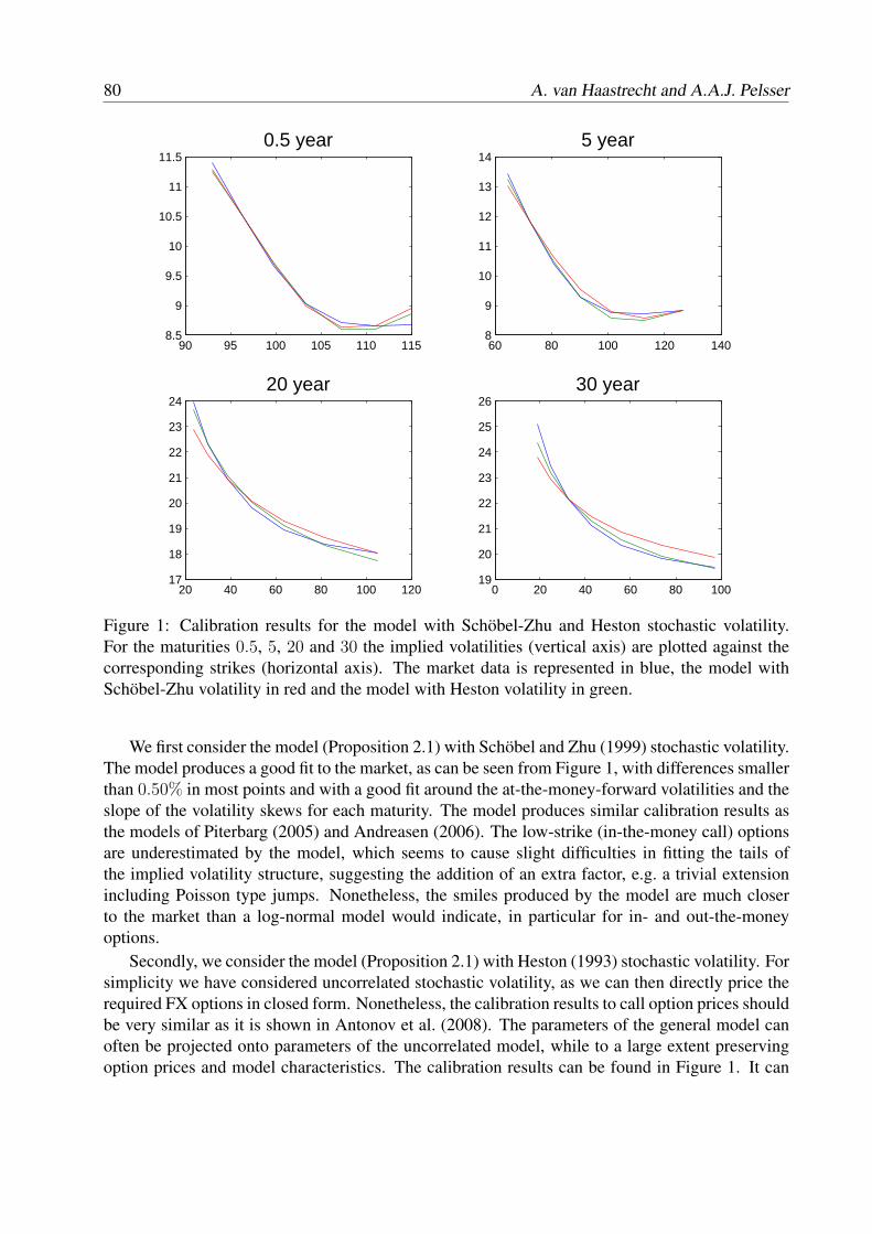
80 A. van Haastrecht and A.A.J. Pelsser
90 95 100 105 110 1158.5
9
9.5
10
10.5
11
11.50.5 year
60 80 100 120 1408
9
10
11
12
13
145 year
20 40 60 80 100 12017
18
19
20
21
22
23
2420 year
0 20 40 60 80 10019
20
21
22
23
24
25
2630 year
Figure 1: Calibration results for the model with Schobel-Zhu and Heston stochastic volatility.For the maturities 0.5, 5, 20 and 30 the implied volatilities (vertical axis) are plotted against thecorresponding strikes (horizontal axis). The market data is represented in blue, the model withSchobel-Zhu volatility in red and the model with Heston volatility in green.
We first consider the model (Proposition 2.1) with Schobel and Zhu (1999) stochastic volatility.The model produces a good fit to the market, as can be seen from Figure 1, with differences smallerthan 0.50% in most points and with a good fit around the at-the-money-forward volatilities and theslope of the volatility skews for each maturity. The model produces similar calibration results asthe models of Piterbarg (2005) and Andreasen (2006). The low-strike (in-the-money call) optionsare underestimated by the model, which seems to cause slight difficulties in fitting the tails ofthe implied volatility structure, suggesting the addition of an extra factor, e.g. a trivial extensionincluding Poisson type jumps. Nonetheless, the smiles produced by the model are much closerto the market than a log-normal model would indicate, in particular for in- and out-the-moneyoptions.
Secondly, we consider the model (Proposition 2.1) with Heston (1993) stochastic volatility. Forsimplicity we have considered uncorrelated stochastic volatility, as we can then directly price therequired FX options in closed form. Nonetheless, the calibration results to call option prices shouldbe very similar as it is shown in Antonov et al. (2008). The parameters of the general model canoften be projected onto parameters of the uncorrelated model, while to a large extent preservingoption prices and model characteristics. The calibration results can be found in Figure 1. It can

Generic pricing of FX, inflation and stock options 81
be seen that the model again produces a very good fit to the market, with differences now evensmaller than 0.30% in most points and with excellent fits across moneyness and maturities. Itseems that Heston (1993) model is slightly better in fitting extreme/convex FX skew: in a way it isable to capture both the volatility part of the at-the-money prices, as well as the extremes of the in-and out-the-money prices. Alternatively, one can argue that the addition of an extra factor is stillneeded for the pricing of certain exotic options (e.g. see Fouque et al. (2000)), a discussion whichis, however, beyond the scope of this article.
It is shown in Piterbarg (2005) and Andreasen (2006), that it is of crucial importance to takethe FX skew into account for the pricing and managing of exotic FX structures like PRDCs (powerreverse dual contracts) or cliquets. Therefore, since the skews/smiles generated by our stochasticvolatility models are much closer to the market than the skews/smiles produced by a log-normalmodel, we can conclude that our stochastic volatility models (Proposition 2.1) are better suitedto price and manage these exotic FX structures. Finally, though the models of Piterbarg (2005)and Andreasen (2006) account for the FX skew, our model stands out as we model stochasticvolatility (versus local volatility used in Piterbarg (2005)) and stochastic interest rates, whilst weallow all driving model factors to be instantaneously correlated with each other (versus independentGaussian rates used in Andreasen (2006)). Having this flexibility yields a realistic model, which isof practical importance for the pricing and hedging of options with a long-term FX exposure.
5. CONCLUSION
We have introduced a generic model incorporating stochastic interest rates and stochastic volatilityunder a full correlation structure of all driving model factors, with closed-form pricing formulas forvanilla options and which is able to incorporate the markets implied volatility structures. Due to theflexibility to correlate the underlying FX/Inflation/Stock-index with both the stochastic volatilityand the stochastic interest rates, our approach yields a realistic model, which is of practical impor-tance for the pricing and hedging of options with a long-term exposure. Furthermore, closed-formpricing of vanilla FX, Inflation and stock options is a big advantage for the calibration (and sensi-tivity analysis) of the model. Using Fourier methods, we have shown how vanilla call/put options,forward starting options, year-on-year inflation-indexed swaps and inflation-indexed caps/floorscan be valued in closed-form. Hereby, it must be noted that our model can cover Poisson typejumps with a trivial extension. Under Schobel and Zhu (1999) stochastic volatility, using its affineproperties, we were able to derive the corresponding characteristic functions in closed-form. Un-der Heston (1993) stochastic volatility, the characteristic functions can only be derived explicitlyunder special zero correlation assumptions. Nonetheless, as an alternative, one can use this resultas a control variate for the general model, see van Haastrecht and Pelsser (2008). Our model canbe used for multi-asset purposes (e.g. interest rates, FX, inflation, equity, commodities) and is fastenough for the real life risk management of big portfolios of such products. We think it is par-ticularly suitable for the pricing and hedging of long-dated multi-currency structures (e.g. hybridTARN options, variable annuities, inflation LPI options and PRDC FX swaps) which are sensitiveto both future interest rates evolutions as well as movements from the underlying index and/orcorresponding volatility smiles.

82 A. van Haastrecht and A.A.J. Pelsser
References
J. Andreasen. Closed form pricing of FX options under stochastic rates and volatility. 2006. GlobalDerivatives Conference.
A. Antonov, M. Arneguy, and N. Audet. Markovian projection to a displaced volatility Hestonmodel. http://ssrn.com/abstract=1106223, 2008.
S. Bakshi, C. Cao, and Z. Chen. Empirical performance of alternative option pricing models.Journal of Finance, 52:2003–2049, 1997.
S. Bakshi, C. Cao, and Z. Chen. Pricing and hedging long-term options. Journal of Econometrics,94:277–318, 2000.
D. Brigo and F. Mercurio. Interest Rate Models - Theory and Practice. Springer Finance, 2006.
O. Caps. On the valuation of power-reverse duals and equity-rates hybrids. 2007. http://www.mathfinance.com/workshop/2007/papers/caps/handouts.pdf.
P. Carr and D.B. Madan. Option valuation using the fast fourier transform. Journal of Computa-tional Finance, 2:61–73, 1999.
D. Duffie, J. Pan, and K. Singleton. Transform analysis for affine jump diffusions. Econometrica,68:1343–1376, 2000.
D. Duffie, D. Filipovic, and W. Schachermayer. Affine processes and applications in finance.Annals of Applied Probability, 13:984–1053, 2003.
A. Feuerverger and A.C.M. Wong. Computation of value-at-risk for nonlinear portfolios. Journalof Risk, 3(1):37–55, 2000.
J. Fouque, G. Papanicolau, and R. Sircar. Derivatives in Financial Markets with Stochastic Volatil-ity. Cambridge University Press, 2000.
H. Geman, E. Karoui, and J.C. Rochet. Changes of numeraire, changes of probability measuresand pricing of options. Journal of Applied Probability, 32:443–548, 1996.
P. Glasserman. Monte Carlo Methods in Financial Engineering. Springer Verlag, 2003.
S.L. Heston. A closed-form solution for options with stochastic volatility with applications to bondand currency options. Review of Financial Studies, 6:327–343, 1993.
G. Hong. Forward smile and derivatives pricing, 2004. http://www-cfr.jbs.cam.ac.uk/archive/PRESENTATIONS/seminars/2004/hong.pdf.
J. Hull and A. White. One factor interest rate models and the valuation of interest rate derivativesecurities. Journal of Financial and Quantitative Analysis, 28(2):235–254, 1993.
R. Jarrow and Y. Yildirim. Pricing treasury inflation protected securities and related derivativesusing an HJM model. Journal of Financial and Quantitative Analysis, 38(2):409–430, 2003.

Generic pricing of FX, inflation and stock options 83
S. Kruse. Pricing of inflation-indexed options under the assumption of a lognormal inflation indexas well as under stochastic volatility. http://ssrn.com/abstract=948399, 2007.
R. Lee. Option pricing by transform methods: extension, unification and error control. Journal ofComputational Finance, 7:51–86, 2004.
A. Lewis. A simple option formula for general jump-diffusion and other exponential Levy pro-cesses. http://ssrn.com/abstract=282110, 2001.
R. Lord and C. Kahl. Optimal Fourier inversion in semi-analytical option pricing. Journal ofComputational Finance, 10(4):1–30, 2007.
V. Lucic. Forward-start options in stochastic volatility models. Wilmott Magazine, 5:72–75,September 2003.
F. Mercurio and N. Moreni. Inflation with a smile. Risk, 19(3):70 –75, March 2006.
A.A.J. Pelsser. Efficient Methods For Valuing Interest Rate Derivatives. Springer Finance, 2000.
V. Piterbarg. A multi-currency model with FX volatility skew. http://ssrn.com/abstract=685084, 2005.
R. Schobel and J. Zhu. Stochastic volatility with an Ornstein Uhlenbeck process: An extension.European Finance Review, 4:23–46, 1999.
J. Sippel and S. Ohkoshi. All power to PRDC notes. Risk, 15(11), November 2002.
A.P.C. van der Ploeg. Mathematics with industry (SWI): The ING problem (hybrid Heston-Hull-White model). http://www.math.uu.nl/swi2007/problems-ing, 2007.
A. van Haastrecht and A.A.J. Pelsser. Generic pricing of FX, inflation and stock options un-der stochastic volatility and stochastic interest rates. http://ssrn.com/abstract=1197262, 2008.
A. van Haastrecht, R. Lord, A.A.J. Pelsser, and D. Schrager. Pricing long-maturity equity andFX derivatives with stochastic interest rates and stochastic volatility. http://ssrn.com/abstract_id=1125590, 2008.

84 A. van Haastrecht and A.A.J. Pelsser

EXTENDED ABSTRACTSPOSTER SESSION
85

86

VANNA-VOLGA METHODS APPLIED TO FX DERIVATIVES:FROM THEORY TO MARKET PRACTICE
Frederic Bossens§, Griselda Deelstra†, Gregory Rayee‡ and Nikos S. Skantzos§
§ Forex Quantitative Analysis Research, Fortis Bank, Montagne du Parc 3, Brussels 1000, Belgium†Department of Mathematics,Universite Libre de Bruxelles, boulevard du Triomphe, CP210, Brus-sels 1050, Belgium‡Solvay Brussels School of Economics & Management , Universite Libre de Bruxelles, Avenue F.D.Roosevelt, CP135, Brussels 1050, BelgiumEmail: [email protected], [email protected],
[email protected] and [email protected]
The Foreign Exchange (FX) options market is the largest and most liquid market of options inthe world. First-generation exotics (touch-like options and vanillas with barriers) are becoming sopopular products in FX that it makes imperative for any pricing system to provide a fast and accu-rate mark-to-market pricing for this family of products. Although using the Black-Scholes modelit is possible to derive analytical prices for barrier and touch options, this model is unfortunatelybased on several unrealistic assumptions that render the price inaccurate. In particular, the Black-Scholes model assumes that the foreign/domestic interest rates and the FX-spot volatility remainconstant throughout the lifetime of the option. This is clearly wrong as these quantities changecontinuously. More realistic models should assume that the foreign/domestic interest rates and theFX spot volatility follow stochastic processes that are coupled to the one of the spot. On the otherhand, for short-dated options (typically less than 1 year), assuming constant interest rates doesnormally not lead to significant errors. In this article we assume constant interest rates throughout.
Stochastic volatility models are unfortunately computationally demanding and in most casesrequire a delicate calibration procedure in order to find the value of parameters that allow themodel to reproduce the market dynamics. This has led to alternative ad-hoc pricing techniqueswhich give fast results and are simpler to implement. One such approach is the Vanna-Volga (VV)method which, in a nutshell, consists in adding an analytically derived correction to the Black-Scholes price of the instrument. To do that, the method uses a small number of market quotesfor liquid instruments (typically At-The-Money options, Risk Reversal and Butterfly strategies)and constructs an over-hedge which zeroes out the Black-Scholes Vega, Vanna and Volga of theoption. The choice of this set of Greeks is linked to the fact that they all offer a measure of theoption’s sensitivity with respect to the FX-spot volatility, and therefore the constructed over-hedgeaims to take the smile effect into account. Although the real interest in the approach lies in its
87

88 Bossens et al.
effectiveness at producing reasonable estimates of the market prices of first-generation exotics, asound theoretical justification can only be derived in the case of vanilla options.
In this article we give two interpretations of the VV method to price vanilla options. We showthat the Vanna-Volga price of a vanilla can be seen as a Taylor expansion of the exact vanilla price(with the exact market volatility directly plugged into the B&S formula), in the vicinity of theAt-The-Money-Forward strike. Then we justify the Vanna-Volga method as an approximation toa stochastic volatility model. Next we review two well known VV variations used to price exoticoptions. The first one consists in weighting the Vanna-Volga correction by some function of thesurvival probability, the second one is based on the expected first hitting time argument.
In order to assess the ability of the two above variations of the Vanna-Volga method to reflectmarket prices, we compared them to a large collection of market indicative prices collected fromtrading platforms of the three major FX-option market-makers. In addition to comparing the VVmodels with market prices, we also compared them to a local-volatility model (Dupire), and astochastic volatility model (Heston) calibrated to the smile at maturity and the ATM volatility termstructure. It appears that for FX markets characterized by a dominantly skewed implied volatility,the Dupire model is qualitatively similar to the two Vanna-Volga models (while the Heston onefollows a different trend) and, inversely, in a FX market characterized by a mild skew, the Hestonmodel aligns towards the Vanna-Volga prices while the Dupire one rebels away. However, Hestonand Dupire models (calibrated to the vanilla market) seem less performing (for this dataset) whencompared to the Vanna-Volga method after it has been calibrated. This confirms that calibrating astochastic model to the vanilla market is by no mean a guarantee that exotic options will be pricedcorrectly, as a vanilla market carries no information about the smile dynamics.
In the literature, there is no agreed consensus regarding whether the survival probability orthe expected first hitting time is a better candidate for adjusting the Vanna-Volga recipe to priceexotics. Based on some empirical observations, it is suggested that one uses some function of thesurvival probability. Other market beliefs however favor using a function of the first exit time.Other adjustment possibilities are also suggested, depending on the type of option at hand. Butthere exists no mathematical argument to justify these choices. In this article we discuss a moresystematic procedure to calibrate the Vanna-Volga model. This calibration allows to reproducemarket prices in a better way and ensures no-arbitrage opportunities.
The FX derivatives community, perhaps more than any other asset class, lives on a complexstructure of quote conventions. Naturally, a wrong interpretation of the input market data cannotlead to the correct results. To this end, we have presented some relevant FX conventions regardingsmile quotes and we have tested the robustness of the Vanna-Volga method against the input data.It appears that the values of Vanna and Volga provide a good indication of whether we are in aregion of parameters where the method is very sensitive with respect to its input.

AN ANALYSIS OF THE UNDERWRITING CYCLE FOR NON-LIFE INSURANCECOMPANIES
Rocco Roberto Cerchiara† and Fabio Lamantia†
†Department of Business Science, University of Calabria, Via Bucci 3C, I-87036 Rende (CS), ItalyEmail: [email protected], [email protected]
The European Solvency II project (see CEIOPS (2007)) introduces Solvency Capital Require-ments that capture the overall risk profile of insurance companies, see also Sandstrom (2005). Inthis framework there is a growing need to develop so-called internal risk models to get accurateestimates of liabilities. In the context of non-life insurance, it is crucial to correctly assess riskfrom different sources, such as underwriting risk with particular reference to premium, reservingand catastrophe risks.Especially the underwriting cycle providing additional volatility, can lead to considerable capitalrequirement (see Meyers (2007)). In fact, in adverse development of financial positions, company’smanagement typically tends to raise premium rates or reinsurance, whereas otherwise it increasesdividends or reduces premium rates. See Choi et al. (2002), Cummins and Danzon (1997), Derien(2008), Feldblum (2001), Gron (1994), Higgins and Thistle (2000) for different approaches andextensive analysis.A correct analysis of this phenomena is also significant to understand the evolution of the reservingcycle, which is often correlated, with a lag period, with the underwriting cycle. Indeed it has beenascertained the tendency of insurers to over-estimate technical reserves during the hard part of thecycle, when loss ratios are low, and under-estimate these reserves in the opposite case.The aim of this paper is to correctly model the underwriting cycle for non-life insurance compa-nies.The basic model is derived from Collective Risk Theory. Starting from the idea of Pentikainenet al. (1989) and Daykin et al. (1994), in this paper a dynamic control policy is defined to specifythe relationship between solvency ratio u(t) and safety loadings λ(t), in order to model the Un-derwriting Cycle. In particular a simplified formula of λ(t) is considered; it assumes the form of aone dimensional piecewise linear map in the state variable u(t).Firstly, a deterministic version of this map is analyzed, where aggregate losses x are simply re-garded as a parameter. In this case, a local and a global analysis of u(t) is performed, showing thatthe long run equilibrium of the solvency ratio u(t) can present jump discontinuities as the mainparameters of the model vary. Technically these discontinuities are a consequence of a particulardouble “Border-collision” bifurcation of the underlying map (see Budd et al. (2008) for details),and are related to the crossing of the trajectory of u(t) into regions where the definition of the mapchanges. Stochastic assessments of u(t) conclude the work.
89

90 R.R. Cerchiara and F. Lamantia
References
C.J. Budd, M. DiBernardo, A.R. Champneys, and P. Kowalczyk. Piecewise-smooth dynamicalsystems. Springer, 2008.
CEIOPS. QIS 4. Technical Specifications, 2007.
S. Choi, D. Hardigree, and P. Thistle. The property-liability insurance cycle: A comparison ofalternative models. Southern Economic journal, 68:530–548, 2002.
J-D. Cummins and P. Danzon. Price, financial quality and capital flows in insurance markets.Journal of Financial Intermediation, 6:3–38, 1997.
C. D. Daykin, T. Pentikainen, and M. Pesonen. Practical Risk Theory for actuaries. Chapman andHall, London, 1994.
A. Derien. An empirical investigation of the factors of the underwriting cycles in non-life market.In Proceedings of MAF, Venice, 2008.
S. Feldblum. Underwriting cycles and business strategies. In Proceedings of the Casualty ActuarialSociety, volume LXXXVIII, pages 175–235, 2001.
A. Gron. Evidence of capacity constraint and cycle in insurance markets. Journal of Law andEconomics, 37(2):349–378, 1994.
M. Higgins and P. Thistle. Capacity constraints and the dynamics of underwriting profits. Eco-nomic Inquiry, 38:442–457, 2000.
G. Meyers. The common shock model for correlated insurance losses. Variance, 1(1):40–52, 2007.
T. Pentikainen, J. Rantala, H. Bonsdorff, M. Pesonen, and M. Ruohonen. Insurance solvency andfinancial strength. Insurance Publishing Company, Helsinki, 1989.
A. Sandstrom. Solvency - Models, Assessment and Regulation. Chapman and Hall, London, 2005.

IMPLIED LEVY VOLATILITY
Jose Manuel Corcuera†, Florence Guillaume§, Peter Leoni‡ and Wim Schoutens§
†Department of Mathematics, University of Barcelona, Gran Via de les Corts Catalanes 585, B-08007 Barcelona, Spain§Department of Mathematics, K.U.Leuven, Celestijnenlaan 200 B, B-3001 Leuven, Belgium‡Electrabel NV/SA, Brussels, Boulevard du Regent 8, B-1000 BelgiumEmail: [email protected], [email protected],
[email protected], [email protected]
We introduce the concept of implied Levy volatility, hereby extending the intuitive Black-Scholes implied volatility into a more general context. More precisely, Levy implied time andspace volatility are introduced and a study of the shape of implied Levy volatilities is made.
Model performance is studied by analyzing delta-hedging strategies for the Normal InverseGaussian and the Meixner model, both qualitatively and on historical time-series of the S&P500.
1. IMPLIED BLACK-SCHOLES VOLATILITY
The Black-Scholes model uses geometric Brownian motion to model the diffusion part of the log-return process:
St = S0 exp((r − q − σ2/2)t+ σWt), t ≥ 0.
The Black-Scholes implied volatility is the volatility σ = σ(K,T ) such that the model and marketoption prices coincide.
The concept of implied volatility under the Black-Scholes model is one of the key points ofits success and its widespread use. In fact it gives another, more convenient and robust, way ofquoting plain vanilla European option prices. Over the years, option traders have developed anintuition in this quantity. As it turns out, this model parameter depends on the characteristics of thecontract. More precisely, it depends on the strike price and the remaining lifetime of the option.The precise functional form is called the volatility surface and follows its own dynamics in themarket. This model parameter needs to be adjusted separately for each individual contract giventhe inadequacy of the underlying Black-Scholes model.
By analyzing empirical historical data, it is not hard to see that stock returns tend to be moreskewed and have fatter tails than those the normal distribution can provide. Here a similar conceptis developed but now under a Levy framework and therefore based on distributions that matchmore closely historical returns.
91

92 J. M. Corcuera et al.
2. IMPLIED LEVY VOLATILITY MODELS
The Levy models are obtained by replacing the Wiener distribution modeling the diffusion part ofthe log-return process by a more empirically founded Levy distribution. The Levy space volatilitymodel will arise by multiplying volatility with the underlying Levy process, whereas the Levy timevolatility model will arise by multiplying volatility squared with time:
St = S0 exp((r − q + ωspace)t+ σspaceXt), t ≥ 0,
andSt = S0 exp((r − q + ωtimeσ
2time)t+Xσ2
timet), t ≥ 0,
where E[X1] = 0, Var[X1] = 1, ωspace = − log(φ(−σi)) and ωtime = − log(φ(−i)) where φrepresents the characteristic function of X1: φ(u) = E [exp(iuX1)]. The volatility parameterσspace = σspace(K,T ) and σtime = σtime(K,T ) needed to match the model price with a given marketprice is called the implied Levy space volatility and the implied Levy time volatility, respectively.
3. STUDYING IMPLIED LEVY VOLATILITY SHAPES
By switching from the Black-Scholes world to the Levy world, we introduce additional degrees offreedom which can be used in order to minimize the curvature of the volatility surface. We lookhow Black-Scholes curves are translated into implied Levy volatility curves and vice versa. It isshown that any smiling or smirking Black-Scholes volatility curve can be transformed into a flatterLevy volatility curves under a well chosen parameter set. This gives some evidence to the fact thatthe implied Levy models could lead to flatter volatility curve for more practical datasets. Hence,implied Levy volatility models can be of a particular interest for practitioners facing the problemof pricing barrier options since for the Black-Scholes model, it is not clear which volatility oneshould use (the one of the barrier or the one of the strike).
4. IMPROVING THE DELTA HEDGE
Model performance is studied by analyzing delta-hedging strategies for short term ATM vanillaoptions under the Normal Inverse Gaussian and the Meixner model, both qualitatively and onhistorical time-series of the S&P500. The Levy degrees of freedom can thus be determined suchthat the absolute value of the mean and the square root of the variance of the daily hedging error areminimized. It is shown that using the historical optimal parameters leads to a significant reductionof the variance of the hedging error (amounting to more than 50 percents), which is particularlyattractive for option hedging.

A GEOSTATISTICAL APPROACH FOR DYNAMIC LIFE TABLES.THE EFFECT OF MORTALITY ON REMAINING LIFETIME AND ANNUITIES1
Ana Debon†, Francisco Martınez-Ruiz§ and Francisco Montes§
†Dpto. de Estadıstica e I. O. Aplicadas y Calidad. Universidad Politecnica de Valencia. Spain§Dpt. d’Estadıstica i I. O.. Universitat de Valencia. SpainEmail: [email protected], [email protected], [email protected]
Our contribution consists of applying geostatistical techniques for estimating the dependence struc-ture of the mortality data in a dynamic life table and for predicting purposes. We compare the per-formance of this new approach with the classic Lee-Carter model with one and two terms and withan enlarged version including the influence of the year of birth (cohort). Additionally, we obtainbootstrap confidence intervals for predicted qxt resulting from applying both methodologies, andwe study their influence on the predictions of e65t and a65t.
1. A BRIEF DESCRIPTION
Static life tables do not take into account the fact that mortality progresses over the years. Theconcept of a dynamic life table seeks to solve this problem by jointly analyzing mortality datacorresponding to a series of consecutive years. This approach allows the calendar effect influenceon mortality to be studied. A sample of the models developed for graduating dynamic tables canbe found in Tabeau et al. (2001), Pitacco (2004), Wong-Fupuy and Haberman (2004), Debon et al.(2006). Most of them adapt traditional laws to the new situation and all them share a commonhypothesis: they consider the observed measures of mortality as independent across ages and overtime. As Booth et al. (2002) point out, it is difficult to hold such a hypothesis when looking at thegraph of the residuals obtained after the adjustment with any of these models.
Geostatistical techniques were designed for the analysis of data which were very far from whata dynamic table represents (Matheron 1975). This distance is only apparent as a dynamic tablecan actually be considered as a set of data over a rectangular grid equally spaced both vertically,for age, and horizontally, for year. The aim of Geostatistics is to model the dependence structureamong neighbours, which requires defining a neighbourhood relationship as well as a distance.
1This work has been supported by grants from the MEyC (Ministerio de Educacion y Ciencia, Spain, projectMTM2007-62923 and project MTM2008-05152) and by a grant from the Generalitat Valenciana (grant No.GVPRE/2008/103)
93

94 A. Debon et al.
They are straightforward in the case of spatial data but also possible in other kind of data. Theanalysis of sudden infant death syndrome (SIDS) in North Carolina in Cressie (1993), as well asthe analysis using spatial techniques of the 1970 US Draft Lottery (Mateu et al. 2004), supportthis assessment. Moreover, as in previous studies, we will show that these methods provide bettersolutions than the classical methods since they simultaneously take into account the effect of ageand time, while the others treat both effects separately.
This works introduces the original Lee-Carter model with one and two time terms and theLee-Carter age-period-cohort model, derived from the original one but adding a second term forcollecting the influence of cohort over mortality, and also provides an introduction to geostatisticalmethodology, including a brief description of the median polish algorithm that will be used for es-timating the deterministic trend of the geostatistic model proposed, namely a Gneiting model. Thebootstrapping techniques used for obtaining confidence intervals are briefly presented. The sevenmodels, three Lee-Carter and four median polish models, are applied for modeling the mortalitydata in Spain for the period 1980-2003 and a range of age from 0 to 99. As the crude estimates ofqx,2004 and qx,2005 are known, the predictions for qx,2004 and qx,2005 are obtained in order to measurethe goodness of prediction for each model. Confidence intervals for the prediction of residual lifeexpectancy, e65t, and the annual rates, a65t, for t = 2004, . . . , 2023, are calculated. Finally, wediscuss the conclusions that can be drawn from comparing the results for different models.
References
H. Booth, J. Maindonald, and L. Smith. Applying Lee-Carter under conditions of variable mortalitydecline. Population Studies, 56(3):325–336, 2002.
N. Cressie. Statistics for Spatial Data, Revised Edition. John Wiley, New York, 1993.
A. Debon, F. Montes, and R. Sala. A comparison of models for dynamical life tables. Applicationto mortality data of the Valencia region (Spain). Lifetime Data Analysis, 12(2):223–244, 2006.
J. Mateu, F. Montes, and M. Plaza. The 1970 US draft lottery revisited: a spatial analysis. JRSSSeries C (Applied Statistics), 1(53):219–229, 2004.
G. Matheron. Random Sets and Integral Geometry. Wiley, New York, 1975.
E. Pitacco. Survival models in dynamic context: a survey. Insurance: Mathematics & Economics,35(2):279–298, 2004.
E. Tabeau, A. van den Berg Jeths, and C. Heathcote (Eds). A Review of Demographic ForecastingModels for Mortality. Forecasting in Developed Countries: From description to explanation.Kluwer Academic Publishers, 2001.
C. Wong-Fupuy and S. Haberman. Projecting mortality trends: Recent developments in the UnitedKingdom and the United States. North American Actuarial Journal, 8(2):56–83, 2004.

PRICING AND HEDGING ASIAN BASKET SPREAD OPTIONS
Griselda Deelstra§, Alexandre Petkovic† and Michele Vanmaele‡
§Universite Libre de Bruxelles, Departement de Mathematiques, ECARES and Solvay BrusselsSchool of Economics & Management†Universite Libre de Bruxelles, ECARES‡Universiteit Gent, Department of Applied Mathematics and Computer ScienceEmail: [email protected], [email protected],
We consider a security market consisting of m risky assets and a risk-less asset with rate ofreturn r. We assume that under the risk-neutral measure Q the price process dynamics are givenby
dSjt = rSjtdt+ σjSjtdBjt,
where Bjt : t ≥ 0 is a standard Brownian motion associated with asset j. Further we assumethat the asset prices are correlated according to
cov(Bjtv , Bits) = ρjimin(tv, ts).
Given the above dynamics, the price of the jth asset at time ti equals
Sjti = Sj(0)e(r−σ2j2
)ti+σjBjti .
With this in hand we can define an Asian basket spread as
V =1
n
n∑i=1
m∑j=1
εjajSjti ,
where aj is the weight given to asset j and εj its sign in the spread. We assume that εj = 1 forj = 1, . . . , p, εj = −1 for j = p + 1, . . . ,m, where p is an integer such that 1 ≤ p ≤ m − 1 andt0 < t1 < t2 < · · · < tn = T . The price of an Asian basket spread with exercise price K at t0 = 0can be defined as
e−rTEQ(V −K)+, (1)
95

96 Deelstra et al.
with (x)+ = max(x, 0) and where EQ represents the expectation taken with respect to the risk-neutral measure Q.
Examples of such contracts can be found in the energy markets. The basket spread part mayfor example be used to cover refinement margin (crack spread) or the cost of converting fuel intoenergy (spark spread). While the Asian part (the temporal average) avoids the problem common tothe European options, namely that speculators can increase gain from the option by manipulatingthe price of the assets near maturity.
Since the density function of a sum of non-independent log-normal random variables has noclosed-form representation, there is no closed-form solution for the price of a security wheneverm > 1 or n > 1 within the Black and Scholes framework. Therefore one has to use an approxima-tion method when valuating such a security. It is always possible to use Monte Carlo techniques toget an approximation of the price. However, such techniques are rather time-consuming. Further-more financial institutions also need approximations of the hedge parameters in order to control therisk, which further increases the computation time. This explains why the research for a closed-form approximation has become an active area.
In the first part of the paper we derive approximation formulae for expression (1) using comono-tonic bounds. Traditionally comonotonic approximations were used to derive bounds for the pricesof Asian and basket options. To the best of our knowledge this is the first time that comonotonicityis used to derive approximations to the price of basket spread and Asian basket spread options. Us-ing the theory of comonotonicity we derive four different approximations: the upper, the improvedupper, the lower and the intermediary bound.
In the second part of the paper we try to approximate the security price with the help of momentmatching techniques. In this paper we improve two well known moment matching approximations,namely the hybrid moment matching and the shifted log-normal approximation.
We find that the comonotonic improved upper bound offers a good approximation of the priceof spread options. We try several approximation methods for basket spread options and find that acombination of hybrid moment matching combined with the comonotonic improved upper boundand shifted log-normal moment matching seems to work best. Finally, for the approximation ofAsian basket spread options we recommend the use of hybrid moment matching combined withthe comonotonic improved upper bound.
We explain which method should be used depending on the basket characteristics. We alsoprovide closed-form formulae for the Greeks of our selected approximation techniques. Finally,we explain how our results can be adapted in order to deal with options written in foreign currency(compo and quanto options).

RISK INDIFFERENCE PRICING AND BACKWARD STOCHASTIC DIFFERENTIALEQUATIONS
Xavier De Scheemaekere
Solvay Brussels School of Economics and Management, Universite Libre de Bruxelles, AvenueF.D. Roosevelt, 50, CP 145/1, Brussels 1050, BelgiumEmail: [email protected]
In a complete market, it is well-known that there is a unique linear arbitrage-free pricing rulefor a contract with payoff G at maturity. This price is the expectation of the discounted payoff Gwith respect to the so-called equivalent martingale measure.
Assuming more realistically that markets are incomplete, the situation becomes more com-plicated. There are infinitely many equivalent martingale measures which might be used in thepricing formula. The no-arbitrage assumption provides a set of equivalent martingale measuresand an interval of arbitrage-free prices. There is no exact replication recipe to provide a uniqueprice. One possibility for a trader is to charge a super-replication (super-hedging) price for sellingan option so that he can trade to eliminate all risks. However, this price is usually forbiddinglyhigh. For example, the super-replication price for a European option is the trivial upper boundof the no-arbitrage interval. In the most common example of a call option, the super-hedgingstrategy is to buy and hold the underlying and therefore the price of the call is equal to the initialstock price, which is excessively expensive and wipes out any advantage that an insurance contractshould have, i.e., intrinsic leverage.
In other words, the gap between upper (seller) and lower (buyer) hedging price is too wide.Since super-hedging is not a realistic solution under such circumstance, the trader is restricted tocharging a reasonable price, finding a partial hedging strategy according to some optimality crite-rion, and bearing some risks in the end.
There are two major approaches that have been developed for pricing and hedging in incom-plete markets. One is to pick a specific martingale measure for pricing according to some optimal-ity criterion, and the other is utility-based derivative pricing. In brief, the pitfall of the first methodis that it does not provide financially reasonable hedging strategies, whilst the second one requiresthe trader to explicitly write down his utility function, which is quite unusual in practice.
97

98 X. De Scheemaekere
In this work, we investigate a pricing formula in incomplete markets based on the risk indiffer-ence principle. We replace the criterion of maximizing utility by minimizing risk exposure becausethe latter is more often used in practice and because it is a natural extension to the idea of pricingand hedging in complete markets. Because the theory of pricing fundamentally relies on hedgingrisk, it is interesting to have a pricing principle directly based on risk. Moreover, risk indifferencepricing preserves the advantage of utility indifference pricing, mainly, its economic justification,while avoiding its limitations, essentially, the lack of explicit calculations outside exponential util-ity models. The idea is that the trader buys or sells the option for an amount such that with activehedging his risk exposure will not increase at expiration.
Using a dual characterization of risk measures, we show that a risk indifference pricing problemreduces to two (zero-sum) stochastic differential games. Then we solve these stochastic differentialgames by means of backward stochastic differential equation (BSDE) theory and find an explicitformula for the risk indifference price. We follow the spirit of Øksendal and Sulem (Risk indif-ference pricing in jump diffusion markets, to appear in Mathematical Finance 2009) who study asimilar risk indifference pricing problem. Importantly, our (stochastic analysis) approach does notimpose Markovian assumptions on the coefficients – it is a well-known benefit of BSDE over PDEtechniques – and it encompasses the case of dynamic (time-consistent) risk measures.
We define the seller’s dynamic risk indifference price priskt as the payment that makes the riskinvolved for the seller of a contract equal to the risk involved if the contract is not sold, at all times.Assume that S is the stock price process, g is the payoff function of the (path-dependent) optioncontract and λ and h are functions determined by the penalty function (of the dual representation)of the risk measure. Then, for an optimal θ∗t , we prove that the risk indifference price priskt satisfies
priskt =RGt −R0
t
Kθ∗t
where Kθ is the process defining the set of equivalent martingale measures and (RGt , Zt) is the
solution of the following BSDE:
RGt = g(S)− h(Y )−
T∫t
λ(t, y, θ∗t )dt−T∫t
ZtdWt,
Y being a vector process that includes S and Kθ. Similarly, (R0t , Zt) is the solution of the above
BSDE with terminal value equal to −h(Y ).
Our results show that the choice of the penalty function is crucial for it determines the shapeof the risk measure, the optimal martingale measure and the size of the price interval. Indeed, thedifference between RG
t and R0t depends essentially on the functions λ and h, and the optimal θ∗t
depends on λ as well.

SYNDICATED SECURED LOAN DERIVATIVES:MODELLING OF LCDS AND PRICING OF LCDX TRANCHES
Peter Dobranszky† and Wim Schoutens§
†Finalyse SA, Rue de Suisse 18, 1060 Brussels, Belgium, FORTIS Bank, Risk Management Mer-chant Banking, Belgium and KULeuven, Department of Mathematics, Belgium§Department of Mathematics, KULeuven, Celestijnenlaan 200 B, 3001 Leuven, BelgiumEmail: [email protected], [email protected]
Although the market is busy today working on the bullet LCDS contract to remove the cancellationfeature from syndicated secured loan derivatives, in their current form LCDSs and LCDX tranchesare still exposed to the cancellation risk. Until recently, in lack of a proper modelling framework,market practitioners neglected the cancellation risk and they priced and hedged these products assimple CDSs and CDO tranches.
However, as we show in this paper, it is more than important to take into account the can-cellation risk when marking-to-market and hedging syndicated secured loan derivatives. This isespecially true in the current market situation. We present easy and robust techniques to model thecancellation feature. We focus on modelling and pricing of syndicated secured loan derivatives.This incorporates the joint modelling of CDS and LCDS spreads (single-name derivatives) as wellas the pricing and hedging of LCDX tranches (multi-name derivatives).
1. SINGLE-NAME DERIVATIVES
The major difficulty when modelling syndicated secured loan derivatives is to retrieve the impliedcancellation probabilities from traded market instruments. In Dobranszky (2008) we show thatin spite of some market believes these implied cancellation probabilities can hardly be derivedsolely from CDS and LCDS spreads. This happens because the fair spread of an LCDS is notsignificantly sensitive to the cancellation rate, which amortizes the credit leg and the fee leg closelyequally. However, the risky annuity used for marking-to-market LCDS contracts is more thansensitive to the cancellation rate. Therefore, even if the implied cancellation probabilities canhardly be derived solely from CDS and LCDS spreads, an assumption about the cancellation rateis essential for marking-to-market LCDS contracts. For the purpose of the analysis a new reduced-form model is introduced, which copes with correlated default and cancellation intensities as wellas with correlated default intensity and stochastic recovery rates.
99

100 P. Dobranszky and W. Schoutens
2. MULTI-NAME DERIVATIVES
In Dobranszky and Schoutens (2008), a new multi-name LCDS model is introduced, which cancope with the problem of implied cancellation probabilities and may help in hedging LCDXtranches. In this paper, the class of one-factor models is extended with cancellation feature. Weanalyse various Levy copulas applied for pricing LCDX tranches. Numerical experiments are pre-sented. In Dobranszky and Schoutens (2009), we show how the cancellation rates can be calibratedfrom super senior tranche quotes. Furthermore, we carry out a historical analysis to show, that themodel extended with the cancellation feature produces more stable and flatter base correlationcurves, as well as that the index hedge implied by the model results in smaller standard deviationof the daily PnL comparing to the deviation implied by the hedge disregarding from cancellation.We analyse the impact of cancellation on the marking-to-market and we address the problem ofhedging the cancellation risk.
References
P. Dobranszky. Joint modelling of CDS and LCDS spreads with correlated default and prepaymentintensities and with stochastic recovery rate. Technical Report 4, K.U.Leuven, 8 2008.
P. Dobranszky and W. Schoutens. Generic Levy one-factor models for the joint modelling ofprepayment and default: Modelling LCDX. Technical Report 3, K.U.Leuven, 6 2008.
P. Dobranszky and W. Schoutens. Do not forget the cancellation - Marking-to-market and hedgingLCDX tranches. Technical Report 2, K.U.Leuven, 3 2009.

PORTFOLIO INSURANCE, IS IT TRUE THAT COMPLEXITY LEADS TO BETTERPERFORMANCES?
Elisabete Mendes Duarte† and Jose Alberto Soares da Fonseca§
†School of Technology and Management, Polytechnic Institute of Leiria, Morro do Lena, Alto doVieiro, 2401 951, Leiria, Portugal§Faculty of Economics Coimbra University, Av. Dias da Silva, n165, 3004 511 Coimbra, PortugalEmail: [email protected], [email protected]
In the last twenty five years, a considerable number of Portfolio Insurance methods have emergedin Financial Markets. Portfolio Insurance methods fit a group of techniques of different complexitydegrees. Since Leland (1980) and Rubinstein and Leland (1981), this strategy, deeply rooted inthe options valuation theory, has been developed in the sense of guaranteeing the same goals withthe simplest techniques. The importance of Portfolio Insurance, as a hedging strategy, arises fromthe asymmetric risk preferences of investors. Portfolio Insurance allows investors to limit theirdownside risk, while retaining exposure to higher returns.
The aim of this article is to discover if it is necessary to implement the more complex Port-folio Insurance techniques or if the simplest ones provide good performances. To achieve ourpurpose, we apply three Portfolio Insurance strategies: the Stop-Loss strategy, the CPPI (ConstantProportion Portfolio Insurance) and the OBPI (Option Based Portfolio Insurance).
Portfolio Insurance techniques have their roots in the Black and Scholes option pricing theory.In Black and Scholes (1973) a non-arbitrage argument is used to derive the model equation. Thisarbitrage argument can also be used to synthetically create options. OBPI was the first proposedstrategy of Portfolio Insurance, see Leland (1980) and Rubinstein and Leland (1981). OBPI usesthe Black and Scholes options valuation model to create a continuously adjusted synthetic Euro-pean put. The Stop Loss strategy, in its most basic version, settles on a simple proposition: afloor (F ) at a maturity 1 is fixed, which is the minimum value allowed to the portfolio. The initialinvestment is fully applied in the stock. The floor present value is periodically compared with theportfolio value. Two different situations may occur: i) If the portfolio value, at time t, is higherthan the floor present value, Pt > Fe−r(1−t), the investment in the stock remains unchanged; ii) Ifthe portfolio value, at time t, is lower or equal to the floor present value, Pt ≤ Fe−r(1−t), the stockis immediately sold out and the investor’s wealth is invested into the risk-free asset.
The CPPI (Constant Proportion Portfolio Insurance) was originally proposed by Perold (1986)and Black and Jones (1987, 1988). The difference at each time t between the portfolio value (Pt)and the floor (Ft) is defined as the cushion. The product of the cushion for a multiple (m), givesus, at time t, the amount to apply in the risky asset, which is called the exposition. Over time, if thegrowth in the risky asset exceeds the risk-free rate of return, the cushion will rise and the investor’s
101

102 E. Duarte and J. Fonseca
wealth should be switched from the risk-free to the risky asset, allowing the investor to retainexposure to higher returns. If the risky asset performance is not so good, the investor’s wealth, inthe rebalancing moments, will be transferred into the risk-free asset, allowing the investor to havea minimum value (floor) on his portfolio.
It is difficult to evaluate the different Portfolio Insurance strategies, because they are not utilitymaximizing and because of the widely spoken asymmetry of the expected returns. As in Garciaand Gould (1987), Bird et al. (1988, 1990) and Benninga (1990), we try to get our answers byempirical simulation against market data.
We choose to test the performance of Portfolio Insurance against actual market data, PSI-20Index and DJ Stoxx 50 index. We have considered the data obtained between January 2003 andDecember 2008. We make cross-section comparisons between portfolios with the same startingvalue and which guarantee the same minimum value at the end of the period.
The Stop-Loss strategy is the one that presents better results when there is a rise in the indices.For the scenario where there is a decrease at the beginning of the year, followed by a gradual rise ofthe indices in the last months, OBPI provides the best results. CPPI seems to be more appropriatein scenarios where there is a big drop in the indices. The Stop-Loss and the CPPI strategies havethe advantage of not using the option valuation theory, which makes these techniques less complex.But, we may not forget that there are scenarios where only OBPI allows obtaining the expectedresults.
We find that the technique performances are path-dependent and are not related to the methodcomplexity degree. We also find that in some market conditions, the simplest techniques providethe best results.
References
S. Benninga. Comparing portfolio insurance strategies. Finanzmarkt und Portfolio Management,4(1):20–30, 1990.
R. Bird, D. Dennis, and M. Tippett. A stop loss approach to portfolio insurance. Journal ofPortfolio Management, 15(1):35–40, 1988.
R. Bird, R. Cunningham, D. Dennis, and M. Tippett. Portfolio insurance: a simulation underdifferent market conditions. Insurance: Mathematics and Economics, 9:1–19, 1990.
F. Black and R. Jones. Simplifying portfolio insurance. Journal of Portfolio Management, pages48–51, Fall 1987.
F. Black and R. Jones. Simplifying portfolio insurance for corporate pension plans. Journal ofPortfolio Management, pages 33–37, Summer 1988.
C.B. Garcia and F.J. Gould. An empirical study of portfolio insurance. Financial Analysts Journal,43(4):44–54, July-August 1987.
A.F. Perold. Constant proportion portfolio insurance. Technical Report 97-011, Harvard BusinessSchool, 1986.

FUNDING OF A HYBRID PENSION SCHEME
Denise Gomez-Hernandez†, Iqbal Owadally§ and Steven Haberman§
†Facultad de Contadurıa y Administracion, Universidad Autonoma de Queretaro, Cerro de lasCampanas s/n, Col. Las Campanas, C.P. 76010, Queretaro, Qro. Mexico.§Faculty of Actuarial Science and Insurance, Cass Business School, 106 Bunhill Row, LondonEC1Y 8TZ, England.Email: [email protected], [email protected], [email protected]
A Hybrid Pension Scheme, called the Modified Contribution (MC), is proposed for an individualaccumulating a fund with variable contributions based on a pre-defined target. The aim of thiswork is to consider the effects of this MC fund on: 1) the value of deficits through time, 2) thefund and contribution variance and 3) the asset allocation through time which minimises the totalfuture cost.
1. METHODOLOGY
The Modified Contribution model assumes an individual starting a pension scheme at age 25 (time0) and retiring at age 65 (time 40). To simplify our model salary growth is not modelled. That is,the projected final salary at retirement is assumed to be equal to 1. The only source of unpredictableexperience that is considered in this model is through volatile rates of return. Then, the MC pensionfund is simulated by making use of the following recursion:
ft+1 = (ft + Ct)(1 + it+1) (1)
where it+1 is the rate of investment return in year (t, t + 1) which is modelled considering twomethods: the bootstrap sampling method with historical data for the period 1899 to 2001 and adynamic asset allocation by assuming the alternative model described in Vigna and Haberman(2001).The contribution in equation 1 that should be paid by the individual is as follows:
Ct = c + St (2)
where c is a constant contribution calculated as a notional Defined Benefit (DB) scheme whichprovides a target benefit of 2/3 of final salary and St the adjustment to the contribution assumedto follow two methods which are compared in this work: the spreading described by Dufresne(1988), and the modified spreading (MS) developed by Owadally (2003)1.
1The interested reader should refer to Gomez-Hernandez (2008) for a full description of the model.
103

104 D. Gomez-Hernandez et al.
2. RESULTS
The main results of this work are as follows. First, that when an individual accumulates a ModifiedContribution pension fund (MC), its value closely matches the value of the pre-defined target underthe modified spreading method (MS). That is, the value of the deficits through time are closer tozero when assuming the MS than when assuming the spreading.Second, the individual would prefer to adjust the value of his or her contributions by assuming themodified spreading method as the trade off between the volatility of the fund and the contributioncan be decreased. That is, under the MS there is a choice on the value of the trade off between thevariance of the fund and contribution. Then, depending on the individual’s degree of risk aversion,an optimal choice of the variance can be made.Third, a more conservative asset allocation through the working life of an individual than the so-called ’lifestyle’ investment strategy, is found to give a smaller value of the total future cost withinthe fund of an individual. That is, regardless of the two methods assumed to adjust the value ofthe contributions, the percentage of the fund that should be invested in a high-risk asset, should begradually increased till the end of the working life of the individual, in order to minimise the totalfuture cost. This percentage is found to be smaller under the MS than under the spreading method.
References
D. Dufresne. Moments of pension contributions and fund levels when rates of return are random.Journal of the Institute of Actuaries, 115:535–544, 1988.
D. Gomez-Hernandez. Pension Funding and Smoothing of Contributions. PhD thesis, City Uni-versity, 2008.
M.I. Owadally. Pension funding and the actuarial assumption concerning investment returns.ASTIN Bulletin, 33(2):289–312, 2003.
E. Vigna and S. Haberman. Optimal investment strategy for defined contribution pension schemes.Insurance: Mathematics and Economics, 28:233–262, 2001.

NON-PARAMETRIC ESTIMATION FOR MULTIVARIATE COMPOUND POISSONPROCESSES AND GOODNESS-OF-FIT TESTING
Markus Schicks
Institut fur Mathematische Stochastik, Technische Universitat Braunschweig, Pockelsstraße 14,38106 Braunschweig, GermanyEmail: [email protected]
We present a low-frequency estimator for the copula of the jump distribution of multivariate com-pound Poisson processes. Further we apply this estimator to construct a goodness-of-fit test for thejump copula.
1. MOTIVATION
In this paper, we are investigating multivariate compound Poisson processes (CPPs) with non-negative jumps, i.e. Xt =
∑Nt
k=1 Yk, for all t ≥ 0, where, as usual, Ntt≥0 is a Poisson processwith (known) intensity λ > 0 which is independent of the independent and identically distributedd-dimensional random jumps with distribution F . Based on low-frequency (compound) observa-tions X1, . . . , XN we want to estimate the copula C(x1, . . . , xd) = F (F−1
1 (x1), . . . , F−1d (xd)) of
these jumps. The multivariate estimator is a generalisation of a plug-in estimator for univariateCPPs constructed by Buchmann and Grubel (2003).Recently Esmaeili and Kluppelberg (2008) estimated parametric Levy copulas of CPPs includingan application to insurance risk. To validate copulas several goodness-of-fit tests have been de-veloped, yet no test for jump copulas of CPPs has been constructed. In the following section wepresent an estimator for the jump copula, while Section 3 is devoted to goodness-of-fit testing inthis context. For detailed proofs, examples, and simulation results we refer to Schicks (2009).
2. NON-PARAMETRIC ESTIMATION OF THE JUMP COPULA
We start by denoting the empirical distribution function of the increments ∆Xj = Xj −Xj−1 by
GN(x) =1
N
N∑j=1
I[0,x](∆Xj) for all x ∈ Rd+.
105
106 M. Schicks
Analogously we denote the empirical distribution functions of the margins by G1,N , . . . , Gd,N .Further let Dτ = Dτ ([0,∞]d) denote the Banach space of d-dimensional cadlag-functions withthe norm ‖f‖∞,τ = supx∈[0,∞]d
∣∣e−〈τ,x〉f(x)∣∣.
Let Eλ denote the compound distribution of the standard uniform distribution w.r.t. a Poissonprocess with intensity λ. Further, define the following decompounding operator
Λd(G) :=∞∑k=1
(−1)k+1eλk
λk(G0)∗k,
where G0(.) := G(.)−G(0). Then Λd(G) converges in Dτ , if the Laplace transform of G0 fulfilsG0(τ) < e−λ, which is always the case, if τ is chosen large enough. Now we can define anestimator CN for the jump copula of a CPP, for (x1, . . . , xd) ∈ [0, 1]d, by
CN(x1, . . . , xd) := Λd
(GN(G−1
1,N Eλ, . . . , G−1d,N Eλ)
)(x1, . . . , xd).
For N → ∞ one can then show that the empirical jump copula process converges weakly to acentered Gaussian process in l∞([p, q]d), i.e.
√N(CN(x1, . . . , xd)− C(x1, . . . , xd)
); Z(x1, . . . , xd),
where Z is a Gaussian process, whose covariance structure depends on C only. Moreover, 0 ≤p, q ≤ 1 need to be chosen in such a way, that C has continuous partial derivatives on [p, q]d.
3. GOODNESS-OF-FIT TEST FOR THE JUMP COPULA
The asymptotic behaviour of the empirical jump copula process leads to the following result onKolmogorov-Smirnovs tests for the copulaC0 of F , whereC0 is assumed to have partial derivativeson [p, q]d. Define the following test statistic
T[p,q],N = sup(x1,...,xd)∈[p,q]d
√N∣∣CN(x1, . . . , xd)− C0(x1, . . . , xd)
∣∣.Further let zN,1−α denote the (1 − α)-quantile of TN under C0, then PC
(TN > zN,1−α
)→ 1, as
N →∞, i.e. the Kolmogorov-Smirnov statistic is asymptotically pointwise consistent.
References
B. Buchmann and R. Grubel. Decompounding: an estimation problem for Poisson random sums.Annals of Statistics, 31(4):1054–1074, 2003.
H. Esmaeili and C. Kluppelberg. Parameter estimation of a bivariate compound Poisson process.Preprint, 2008.
M. Schicks. Non-parametric estimation for multivariate compound Poisson processes. Preprint,2009.


De Koninklijke Vlaamse Academie van België voor Wetenschappen en Kunsten coördineert jaarlijks tot 25 wetenschappelijke bijeenkomsten, ook contactfora genoemd, in de domeinen van de natuurwetenschappen (inclusief de biomedische wetenschappen), menswetenschappen en kunsten. De contactfora hebben tot doel Vlaamse wetenschappers of kunstenaars te verenigen rond specifieke thema’s. De handelingen van deze contactfora vormen een aparte publicatiereeks van de Academie. Contactforum “Actuarial and Financial Mathematics Conference” (7-8 februari 2008, Prof. M. Vanmaele) De traditie van de “Actuarial and Financial Mathematics” contactfora werd ook dit jaar verder gezet met de “Actuarial and Financial Mathematics Conference 2009” (kortweg AFMathConf2009) waarbij opnieuw aandacht werd besteed aan de interactie tussen financieel en actuarieel wiskundige technieken. Naast genodigde sprekers en de bijdragen hadden de organisatoren geopteerd voor twee short courses over Solvency II en over Lévy processes en een postersessie. In deze postersessie kregen heel wat jonge onderzoekers de mogelijkheid om hun onderzoeksresultaten voor te stellen aan een ruim publiek bestaande uit academici uit binnen- en buitenland alsook collega's uit de bank- en verzekeringswereld. In deze publicatie vindt u de cursusnota’s van de short course over Lévy processes. Verder twee bijdragen over het prijzen van “death bonds” en van FX, inflatie en aandelenopties onder stochastische rentevoeten en stochastische volatiliteit. Tenslotte bevat deze publicatie de uitgebreide abstracts van de meeste postervoorstellingen.