lecture notes mth5124: actuarial mathematics i
TRANSCRIPT
Lecture Notes
MTH5124: Actuarial Mathematics I
Dr Adrian BauleSchool of Mathematical SciencesQueen Mary University of London
November 3, 2021

2

Contents
0 Prologue 70.1 What is an actuary? . . . . . . . . . . . . . . . . . . . . . . . . . . . . . . . . . . . 70.2 About this course . . . . . . . . . . . . . . . . . . . . . . . . . . . . . . . . . . . . 70.3 About these notes . . . . . . . . . . . . . . . . . . . . . . . . . . . . . . . . . . . . 80.4 Life Tables . . . . . . . . . . . . . . . . . . . . . . . . . . . . . . . . . . . . . . . . 80.5 Books and tables . . . . . . . . . . . . . . . . . . . . . . . . . . . . . . . . . . . . 90.6 Acknowledgements . . . . . . . . . . . . . . . . . . . . . . . . . . . . . . . . . . . 9
1 Compound interest 131.1 Two types of interest . . . . . . . . . . . . . . . . . . . . . . . . . . . . . . . . . . 13
1.1.1 Simple interest . . . . . . . . . . . . . . . . . . . . . . . . . . . . . . . . . . 141.1.2 Compound interest . . . . . . . . . . . . . . . . . . . . . . . . . . . . . . . 14
1.2 Nominal and effective interest rates . . . . . . . . . . . . . . . . . . . . . . . . . . . 161.2.1 Accumulation factor . . . . . . . . . . . . . . . . . . . . . . . . . . . . . . . 161.2.2 Nominal interest rates . . . . . . . . . . . . . . . . . . . . . . . . . . . . . . 171.2.3 Effective interest rates . . . . . . . . . . . . . . . . . . . . . . . . . . . . . 19
1.3 Force of interest . . . . . . . . . . . . . . . . . . . . . . . . . . . . . . . . . . . . . 201.3.1 Time-dependent interest rates . . . . . . . . . . . . . . . . . . . . . . . . . 201.3.2 Force of interest . . . . . . . . . . . . . . . . . . . . . . . . . . . . . . . . . 211.3.3 Special case of constant force of interest . . . . . . . . . . . . . . . . . . . . 23
1.4 Rates of discount . . . . . . . . . . . . . . . . . . . . . . . . . . . . . . . . . . . . 251.4.1 Relation between nominal rates of discount and interest . . . . . . . . . . . . 26
1.5 Discounting Cash Flows or Present Values . . . . . . . . . . . . . . . . . . . . . . . 281.5.1 Discrete cash flows . . . . . . . . . . . . . . . . . . . . . . . . . . . . . . . 29
1.6 Annuities-certain: introduction . . . . . . . . . . . . . . . . . . . . . . . . . . . . . 311.6.1 Immediate annuity . . . . . . . . . . . . . . . . . . . . . . . . . . . . . . . . 311.6.2 Annuity-due . . . . . . . . . . . . . . . . . . . . . . . . . . . . . . . . . . . 311.6.3 Perpetuities . . . . . . . . . . . . . . . . . . . . . . . . . . . . . . . . . . . 321.6.4 Deferred annuities . . . . . . . . . . . . . . . . . . . . . . . . . . . . . . . . 321.6.5 Increasing annuities . . . . . . . . . . . . . . . . . . . . . . . . . . . . . . . 33
1.7 Annuities-certain: more variations . . . . . . . . . . . . . . . . . . . . . . . . . . . 331.7.1 Annuities payable p-thly . . . . . . . . . . . . . . . . . . . . . . . . . . . . 331.7.2 Annuities payable continuously . . . . . . . . . . . . . . . . . . . . . . . . . 341.7.3 Accumulated values . . . . . . . . . . . . . . . . . . . . . . . . . . . . . . . 36
1.8 Continuous cash flows (not examinable) . . . . . . . . . . . . . . . . . . . . . . . . 371.8.1 Continuous cash flow with variable force of interest . . . . . . . . . . . . . . 38
1.9 Repayment of Loans . . . . . . . . . . . . . . . . . . . . . . . . . . . . . . . . . . . 401.9.1 Schedule of payments . . . . . . . . . . . . . . . . . . . . . . . . . . . . . . 401.9.2 Consolidating loans . . . . . . . . . . . . . . . . . . . . . . . . . . . . . . . 41
3

1.10 Investment project appraisal . . . . . . . . . . . . . . . . . . . . . . . . . . . . . . . 43
1.10.1 Payback periods . . . . . . . . . . . . . . . . . . . . . . . . . . . . . . . . . 43
1.10.2 Yield . . . . . . . . . . . . . . . . . . . . . . . . . . . . . . . . . . . . . . . 45
1.11 Immunisation of cash flows . . . . . . . . . . . . . . . . . . . . . . . . . . . . . . . 47
2 Fixed Interest Securities and Other Investments 51
2.1 Fixed Interest Securities . . . . . . . . . . . . . . . . . . . . . . . . . . . . . . . . . 51
2.1.1 Bond Terminology . . . . . . . . . . . . . . . . . . . . . . . . . . . . . . . . 52
2.1.2 Example of a Government Security . . . . . . . . . . . . . . . . . . . . . . . 52
2.1.3 Types of Corporate Bonds . . . . . . . . . . . . . . . . . . . . . . . . . . . 53
2.1.4 Valuation of a Bond . . . . . . . . . . . . . . . . . . . . . . . . . . . . . . . 53
2.2 Cash including Treasury Bills . . . . . . . . . . . . . . . . . . . . . . . . . . . . . . 54
2.3 Inflation Linked Bonds and Real Returns . . . . . . . . . . . . . . . . . . . . . . . . 55
2.3.1 Calculating the Real Rate of Return . . . . . . . . . . . . . . . . . . . . . . 56
2.3.2 Valuation of Index-Linked Bonds . . . . . . . . . . . . . . . . . . . . . . . . 57
2.4 Equities . . . . . . . . . . . . . . . . . . . . . . . . . . . . . . . . . . . . . . . . . 59
2.4.1 Valuation of Shares by Discounting Future Dividends . . . . . . . . . . . . . 60
2.4.2 Characteristics of Preference Shares . . . . . . . . . . . . . . . . . . . . . . 61
2.5 Property . . . . . . . . . . . . . . . . . . . . . . . . . . . . . . . . . . . . . . . . . 62
2.6 Taxation . . . . . . . . . . . . . . . . . . . . . . . . . . . . . . . . . . . . . . . . . 63
2.6.1 Income Tax . . . . . . . . . . . . . . . . . . . . . . . . . . . . . . . . . . . 64
2.6.2 Tax on Capital Gains . . . . . . . . . . . . . . . . . . . . . . . . . . . . . . 64
2.7 The term structure of interest rates . . . . . . . . . . . . . . . . . . . . . . . . . . 66
2.7.1 Spot rates . . . . . . . . . . . . . . . . . . . . . . . . . . . . . . . . . . . . 66
2.7.2 Forward rates . . . . . . . . . . . . . . . . . . . . . . . . . . . . . . . . . . 67
3 Life tables and life-table functions 69
3.1 Lifetime as a random variable . . . . . . . . . . . . . . . . . . . . . . . . . . . . . . 69
3.1.1 Future lifetime . . . . . . . . . . . . . . . . . . . . . . . . . . . . . . . . . . 70
3.2 Basic life-table functions . . . . . . . . . . . . . . . . . . . . . . . . . . . . . . . . 71
3.2.1 Definitions of life-table function . . . . . . . . . . . . . . . . . . . . . . . . 71
3.2.2 Relation between lx and s(x) . . . . . . . . . . . . . . . . . . . . . . . . . 73
3.2.3 Basic life-table functions in terms of lx . . . . . . . . . . . . . . . . . . . . 74
3.3 Force of mortality . . . . . . . . . . . . . . . . . . . . . . . . . . . . . . . . . . . . 76
3.3.1 Relation between µ(x) and other functions . . . . . . . . . . . . . . . . . . 77
3.3.2 The curve of deaths . . . . . . . . . . . . . . . . . . . . . . . . . . . . . . . 78
3.4 Analytical laws of mortality (not examinable) . . . . . . . . . . . . . . . . . . . . . 78
3.5 The expectation of life . . . . . . . . . . . . . . . . . . . . . . . . . . . . . . . . . 79
3.5.1 The complete expectation of life . . . . . . . . . . . . . . . . . . . . . . . . 79
3.5.2 The curtate expectation of life . . . . . . . . . . . . . . . . . . . . . . . . . 80
3.6 Interpolation for fractional ages . . . . . . . . . . . . . . . . . . . . . . . . . . . . . 82
3.6.1 Linear interpolation on s(x) and lx . . . . . . . . . . . . . . . . . . . . . . 83
3.6.2 Derivation of relation between complete and curtate expectations of life . . . 85
3.6.3 Other interpolation schemes on s(x) and lx . . . . . . . . . . . . . . . . . . 86
3.6.4 Assumptions to obtain µ(x) . . . . . . . . . . . . . . . . . . . . . . . . . . 86
3.7 Select mortality . . . . . . . . . . . . . . . . . . . . . . . . . . . . . . . . . . . . . 88
4

4 Life insurance and related functions 954.1 Introduction to life assurance . . . . . . . . . . . . . . . . . . . . . . . . . . . . . . 95
4.1.1 Commutation functions . . . . . . . . . . . . . . . . . . . . . . . . . . . . . 964.2 Whole-life assurance . . . . . . . . . . . . . . . . . . . . . . . . . . . . . . . . . . . 97
4.2.1 Death benefit payable at instant of death . . . . . . . . . . . . . . . . . . . 974.2.2 Death benefit payable at end of year of death . . . . . . . . . . . . . . . . . 99
4.3 Whole-life annuities payable annually . . . . . . . . . . . . . . . . . . . . . . . . . . 1024.3.1 Whole-life annuity-due . . . . . . . . . . . . . . . . . . . . . . . . . . . . . 1024.3.2 Whole-life immediate annuity . . . . . . . . . . . . . . . . . . . . . . . . . . 1044.3.3 Life assurance premiums . . . . . . . . . . . . . . . . . . . . . . . . . . . . 105
4.4 Policies of duration n . . . . . . . . . . . . . . . . . . . . . . . . . . . . . . . . . . 1064.4.1 n-year life assurance for life aged x . . . . . . . . . . . . . . . . . . . . . . 1064.4.2 n-year pure endowment for life aged x . . . . . . . . . . . . . . . . . . . . . 1074.4.3 n-year endowment policy for life aged x . . . . . . . . . . . . . . . . . . . . 1094.4.4 n-year life annuities for life aged x . . . . . . . . . . . . . . . . . . . . . . . 109
4.5 p-thly payments . . . . . . . . . . . . . . . . . . . . . . . . . . . . . . . . . . . . . 1114.5.1 Whole-life assurance paid p-thly . . . . . . . . . . . . . . . . . . . . . . . . 1114.5.2 Whole-life p-thly annuities . . . . . . . . . . . . . . . . . . . . . . . . . . . 1134.5.3 Alternative approximation for A(p)
x . . . . . . . . . . . . . . . . . . . . . . . 115
5

6

Chapter 0
Prologue
0.1 What is an actuary?
“An actuary is someone who expects everyone to be dead on time.” is one definition you canfind on the internet.1 In fact, actuaries do much more than deal with the probabilities of peo-ple dying! In short, they use financial and statistical theories to quantify and manage risk inall areas of business. Traditionally actuaries specialize in consultancy, investment, life and gen-eral insurance or pensions. However, their analytical skills are also increasingly valuable in otherareas—after all, “risk management” is of wide importance in financially turbulent times. Actuar-ies are highly-regarded and (well-paid!) professionals. For more details of career paths, etc., seehttp://www.actuaries.org.uk/becoming-actuary/.
0.2 About this course
The idea of this course is to introduce you to some of the basic mathematical ideas used in actuarialwork. MTH5124 is designed for second or third year undergraduates and assumes a backgroundin basic Calculus and Probability.2 All practicalities about the course itself (timetable, coursework,assessment details), etc., can be found on the course QM+ websitehttp://qmplus.qmul.ac.uk/course/view.php?id=18186.
Important announcements and corrections will also be posted there.The course uses familiar mathematical concepts (e.g., geometric series, probability distributions)
but in an unfamiliar context. I hope you will be interested to see how maths you already know canbe used effectively in the “real world”. However, one of the problems in applying maths to a differentfield is that you often have to learn new terminology, notation, etc. in order to communicate withspecialists in that area. This is certainly the case here; indeed you will soon be introduced to awhole zoo of complicated actuarial symbols and new vocabulary. It is crucial for success that youlearn this “new language” so that the familiar mathematical objects do not become lost in the fogof unfamiliar actuarial terminology.
The course has four main “chapters”:
1. Compound interest: Here we will cover various (interrelated) ways to quantify how compoundinterest is added to a loan/investment. You will learn how to calculate accumulations given theforce of interest (or related parameters) and how to deal with series of payments, in particularannuities-certain and perpetuities.
1A quick search with Google yields a variety of other humorous, and not-so-humorous, definitions as well as moreuseful career descriptions.
2Formal prerequisites are Calculus II and Introduction to Probability.
7

2. Fixed interest securities and other investments: You will learn about the most commonforms of investments and how to value investments using compound interest.
3. Life tables and life-table functions: Life tables are the actuary’s basic tool. You will learnhow to interpret them in order to find various probabilities related to life and death.
4. Life insurance and related functions: Here we will combine material from the first twochapters to deal with situations involving payments (with compound interest) whose valueand/or timing may depend on a person’s survival or death! Life insurance is the classicexample here.
0.3 About these notes
These notes will cover the material in roughly the same order as the lectures but their style willprobably be slightly different. In particular, the printed notes may contain some longer explanationsand extra examples which time prevents me covering in class. The lectures, however will be importantfor emphasizing the main points and giving exam tips—I strongly recommend that you attend or atleast follow the recordings on QM+!
To help you with revision, all important actuarial terms are printed in bold. You must be sureto understand what these mean, both in everyday language (could you explain them to your grand-mother or your next-door neighbour?) and in terms of the associated mathematical formulation.The notes will also contain a number of “examples” and “exercises”. For the former you will findfull details of the working; for the latter (usually) only the answers. A good way to check your ownunderstanding would be to read the text and try the associated exercises (contact me if you haveany difficulty getting the stated answers). I intend the unstarred exercises to correspond roughly tothe Key Objectives for the course (i.e., everyone should be able to do them); starred exercises willbe somewhat harder and should be attempted by those aiming for a high grade.
0.4 Life Tables
The examples in this document are based on the following life tables:
• English Life Table No 17,
• AMC00 mortality table for assured lives.
These are available on the QM+ page for MTH5124. Copies will be provided in the examination.
Full details of mortality tables published by the CMI can be found athttps://www.actuaries.org.uk/learn-and-develop/continuous-mortality-investigation/cmi-mortality-and-morbidity-tables.
The CMI is a subsidiary of the Institute and Faculty of Actuaries, and was previously knownas The Continuous Mortality Investigation. CMI tables relate to the mortality experience of lifeinsurance policyholders and the members of pension schemes.
The English Life Tables represent the mortality experience of the population of England andWales. Tables are published by the Office of National Statistics (ONS); further information onELT17 can be found athttps://www.ons.gov.uk/peoplepopulationandcommunity/birthsdeathsandmarriages/lifeexpectancies-/bulletins/englishlifetablesno17/2015-09-01.
8
0.5 Books and tables
The course is designed to be fairly self-contained and does not follow any one textbook. However,you may find the following useful for background reading:
• S. J. Garrett An Introduction to the Mathematics of Finance (Butterworth-Heinemann);
– cited in these notes as [Gar13].
• J. J. McCutcheon & W. F. Scott An Introduction to the Mathematics of Finance (Butterworth-Heinemann);
– cited in these notes as [MS86].
• D. C. M. Dickson, Mary R. Hardy & Howard R. Waters Actuarial Mathematics for Life Con-tingent Risks (Cambridge University Press);
– cited in these notes as [DHW13].
• A. Neill Life Contingencies (Heinemann);
– cited in these notes as [Nei77].
• N. L. Bowers, H. U. Gerber, J. C. Hickman, D. A. Jones and C. J. Nesbitt Actuarial Mathe-matics (Society of Actuaries);
– cited in these notes as [BGH+97].
0.6 Acknowledgements
These notes have been produced by Jim Webber from notes for the predecessor module MTH6100Actuarial Mathematics, a module which covered a very similar syllabus. Great credit and thanks toDr Rosemary Harris for her excellent work in producing the original draft of the MTH6100 notes.Also thanks to Dr D. Stark and Dr W. Just for their additions and amendments to the notes sincethe original draft. In her original introduction, Dr Harris gave credit to the previous notes of Prof.B. Khoruzhenko and also the work of another previous lecturer, Dr L. Rass.
The changes I have made have been limited, but I take full responsibility for this edition of thenotes and the mistakes and contradictions that students will inevitably find. Please alert me to anymistake that you find by sending an email to: [email protected].
9

10

Bibliography
[Ber89] J. Bernoulli. Tractatus de seriebus infinitis. manuscript, 1689.
[BGH+97] N. L. Bowers, H. U. Gerber, J. C. Hickman, D. A. Jones, and C. J. Nesbitt. ActuarialMathematics. Society of Actuaries, Schaumburg, 1997.
[DHW13] D. C. M. Dickson, M. R. Hardy, and H. R. Waters. Actuarial Mathematics for LifeContingent Risks. Cambridge University Press, Cambridge, 2013.
[Gar13] S. J. Garrett. An Introduction to the Mathematics of Finance. Butterworth-Heinemann,Oxford, 2013.
[Hal93] E. Halley. An estimate of the degrees of mortality of mankind, drawn from the curioustables of the births and funerals at the city of Breslaw, with an attempt to ascertain theprice of annuities upon lives. Philosophical Transactions, 17:596–610, 1693.
[MS86] J. J. McCutcheon and W. F. Scott. An Introduction to the Mathematics of Finance.Butterworth-Heinemann, Oxford, 1986.
[Nei77] A. Neill. Life Contingencies. Heinemann, London, 1977.
[Pac94] L. Pacioli. Summa de Arithmetica. Venice, 1494.
11

12
Chapter 1
Compound interest
The material in this Chapter is covered very well in ([Gar13]). It is also covered in Chapters 1–4 of([MS86].)
1.1 Two types of interest
Often in the course of daily life and business, people need (or choose) to borrow money. For example,you might have a student loan or, later in life, need a mortgage or business loan. On the otherhand, if you happen to have “spare” money you can lend it to a bank, for example, by investing ina savings account or fixed term bond. In general, in all these situations the money lender receives akind of “reward” for lending the money; you can also think of this as the charging of “rent” for theuse of the money.
To be more specific the original loan/investment is called the capital (or principal) and the“reward” to the lender/investor is the interest. The time-dependent value of the investment, i.e.,the original loan plus the interest, is known as the accumulated amount (or accumulation).
Interest is expressed as a rate in two senses: per unit capital and per unit time. In practice,the interest rate is often quoted in percent and usually, but not always the basic time unit is oneyear. Note that “p.a.” is often used as an abbreviation for per annum (i.e., each year). To avoidconfusion you should always state the basic time period when giving an interest rate.
The interest rate on a transaction is affected by various factors including:
• the market rate for similar loans;
• the risk involved in the use to which the borrower puts the money (cf. mortgage loan ratesand unsecured personal loan rates);
• the anticipated rate of appreciation or depreciation in the value of the currency in which thetransaction is carried out (e.g., in times of high inflation the interest is higher).
For the present we assume that interest rates are constant in time and that there is no dependenceon the sum invested. We will later relax the first of these assumptions but the second will remainthroughout the course.
Now let’s consider a concrete example—a savings account with an interest rate of 5% p.a.. Inother words, one gets a return of £5 in one year for each £100 invested. Suppose you were to invest£200 then you could close the account after one year and withdraw £210 made up of the principal(£200) and the interest (£10). But what if the account were kept open for a period of time whichwas longer (or shorter) than one year? In that case we would need to distinguish between simpleinterest and compound interest.
13

1.1.1 Simple interest
For the bank account considered above then, in the case of simple interest, £10 would be addedeach year to your original deposit of £200. In general, the accumulated amount is after one timeunit (n = 1)
Accumulation = P + iP = P (1 + i) (1.1)
After n time units you obtain interest of niP and thus
Accumulation = P + niP = P (1 + ni) (1.2)
where P = principal invested;i = rate of interest;n = duration of investment/loan.
Expression (1.2) applies for all non-negative values of n. The normal commercial practice inrelation to fractional periods of a year is to pay interest on a pro rata basis (i.e., proportional to thetime the account is open). For an account of duration of less than one year it is usual to allow forthe actual number of days the account is held.
What happens when n is greater than 1 year? Imagine investing the £200 of our example fortwo years (again at 5% p.a. simple interest) then after these two years the accumulation will be
£200(1 + 2× 0.05) = £220.
Is there a way to make more money?Yes, you can close this account (Let’s call it account A.) after one year, at which time you will
withdraw £210 [see (1.2)]. Then place this sum on deposit in a new account, say B. When youclose account B after one further year, the sum withdrawn will be £210(1+1× 0.05)=£220.50. Inother words, you will have gained the princely sum of 50p!
The difference here is that, effectively, account B pays interest on the interest already earned.In general, banks do not want people to be frequently opening and closing accounts. (Whilst youmight not bother to do that to gain 50p you probably would for £50,000!) This is one reason why,for periods greater than one year, most bank accounts do not pay simple interest but instead theinterest is compounded...
1.1.2 Compound interest
In this case interest is paid on the previous interest accrued1. After one time unit (n = 1) we havethe same result as for simple interest
Accumulation = P (1 + i). (1.3)
After two time units (n = 2) we also accumulate the interest on the interest accrued in the previoustime period
Accumulation = P (1 + i) + P (1 + i)i = P (1 + i)(1 + i) = P (1 + i)2. (1.4)
The general formula for the accumulated amount thus becomes
Accumulation = P (1 + i)n. (1.5)
Another way to see this is that if An is the accumulation after n time units then An = An−1(1+i) =An−2(1 + i)2 = . . . = A0(1 + i)n, where A0 is the capital invested initially, i.e. P . This argumentobviously holds for integer n; the validity of (1.5) for non-integer n will be established in Section 1.3.
1Here “interest accrued” simply means interest already earned / applied to the account.
14

Exercise 1.1.1: Effect of compound interestConvince yourself that applying compound interest according to (1.5) has the same effect as closing an accountwith simple interest after each time period and reinvesting the money in an account paying the same interest.
Exercise 1.1.2: Compound interest formulaWrite a formal proof of (1.5) for integer n using induction.
From now on, “interest” always means compound interest unless explicitly stated otherwise.However, simple interest calculations (which you should be able to do in your head!) can sometimesbe a useful tool for checking that compound interest results are in the right ballpark. Simpleinterest is a good approximation for compound interest when n and i are small since in that case(1 + i)n ≈ 1 + ni.
Example 1.1.1: Low interest ratesSuppose you invest £1,000 for three years in a bank account which pays interest annually at 1.5% p.a.. Whatis the difference in accumulation if the bank pays compound interest compared to simple interest?
SolutionFor simple interest then, using (1.2),
Accumulation = £1000× (1 + 3× 0.015) = £1045.00. (1.6)
On the other hand, if interest is compounded, then we use (1.5):
Accumulation = £1000× (1 + 0.015)3 = £1045.68. (1.7)
[Unless stated otherwise, you should always give monetary answers rounded to the nearest penny.] So theaccumulation is only 68p greater if compound interest is paid.
In real-life there are many different kinds of transactions such as:
• payment of a series of premiums throughout a given time period in return for a lump sum atthe end of the period;
• mortgage loans, i.e., loans which are made for the specific purpose of house purchase (Theproperty to be purchased usually acts as security for the loan);
• fixed interest securities, such as regular income payments throughout a given time period andan additional lump sum at the end of the period in return for a one-off payment.
Knowledge of compound interest can be useful in comparing the merits of such transactions.
Example 1.1.2: Investment adviceYou have £10,000 to invest now and are being offered £22,500 after ten years as the return from theinvestment. The market rate is 10% p.a. (compound interest). Ignoring complications such as the effect oftaxation, the reliability of the company offering the contract, etc., do you accept the investment?
SolutionInvesting £10,000 for ten years with 10% compound interest will yield
Accumulation = £10000(1 + 0.1)10 = £25937. (1.8)
Since this is more than £22,500 you should reject the offered investment and just put the money in the bank.
Summary of 1.1
Accumulation of P units of money, simple interest: A = P (1 + ni)Accumulation of P units of money, compound interest: A = P (1 + i)n
15

321
i
t
0A13
(a)
321
0
A1A2
(b)
Figure 1.1: Schematic of investment and accumulation in two different scenarios. The PoC (1.10)says that the accumulated amount at t3 is the same in both cases.
1.2 Nominal and effective interest rates
Now we generalize the set-up of the previous section and consider how to define interest rates whenthe interest is compounded more frequently than annually. For example, many bank accounts payinterest monthly or quarterly.
1.2.1 Accumulation factor
Let A(t1, t2) be the accumulated value at time t2 of 1 unit of money invested at time t1. A(t1, t2)is called the accumulation factor and has the following useful properties:
1. A(t, t) = 1 (by definition)
2. Assuming that interest rates don’t depend on the size of the investment, then the accumulationat t2 of an investment of P at t1 is P ×A(t1, t2).
3. In a “consistent” market we expect that the accumulation doesn’t depend on when, or howoften, money is withdrawn and re-invested. This assumption is called the principle of con-sistency (PoC) and implies.
A(t1, t3) = A(t1, t2)A(t2, t3) ∀ t1 ≤ t2 ≤ t3. (1.9)
You may find this easier to understand with the aid of the diagram in Fig. 1.1.
4. From (1.9), it follows that
A(t1, t2) =A(t0, t2)
A(t0, t1)∀ t0 ≤ t1 ≤ t2. (1.10)
Exercise 1.2.1:Check Eq. (1.10).
Suppose the basic unit of time is one year and interest is compounded yearly at constant rate i.Then we have A(0, 1) = (1 + i) or, more generally,
A(t, t+ n) = (1 + i)n (1.11)
where n is (for now) an integer. This statement is just another way of writing (1.5).Now consider what happens if interest is paid more frequently. In this case we can have accu-
mulations over fractional time periods. In general we say that interest is compounded p-thly (orconvertible p-thly) if it is paid p times in each unit time interval, i.e., paid after a “term” of length1/p. For example, in the usual case where the basic unit of time is one year, then p = 4 meansinterest paid quarterly, whereas p = 12 means interest paid monthly.
16

1.2.2 Nominal interest rates
A nominal interest rate is a rate, per unit time, of interest which applies over a different timeperiod. For example, “overnight money” means that a yearly rate of interest is applied daily (i.e.interest is converted into capital daily, but interest is quoted as a rate per annum).
A nominal interest rate of i(p) per basic time unit is defined to mean that interest is compoundedp-thly with an interest rate of i(p)/p in a time interval of length 1/p. Equivalently, we have
A
(t, t+
1
p
)= 1 +
i(p)
p. (1.12)
For example, a nominal interest rate of 12% p.a. compounded monthly (p=12) means an interestrate of 1% per month and therefore an accumulation factor A(t, t+ 1/12) = 1.01.
Note on notation:
• i(p) does not mean i raised to the power p. The brackets are there to remind you that the phere is just a label.
• In fact, a number in brackets to the top right of any actuarial symbol usually tells you aboutthe frequency of payments; we will see other examples later.
• In [MS86] you will find that i(p) is sometimes written as ih where h = 1/p; we will not usethis notation.
Nominal interest rates for different periods (i.e., terms of length 1/p for different p) are oftenquoted in the financial press, for example, see the excerpt from the Financial Times presented inFig. 1.2.
Example 1.2.1: Nominal interest ratesConsider the nominal market interest rates (% p.a.) given in Fig. 1.2. Look at the line labelled “£ Libor”.2
Assuming these interest rates, find the accumulation of an investment of £10,000 on 7.12.16 after (a) onequarter and (b) 1 day (overnight money).
SolutionHere the basic time unit is one year (interest rates are quoted p.a.) but we are considering interest paid afterfractions of this time.(a) p = 4; from the table we have a nominal interest rate of 0.38363% per year which means i(4) = 0.0038363.The accumulated amount is given by
Accumulation = P ×A(
0,1
4
)(1.13)
= £10000×(
1 +0.0038363
4
)[using (1.12)] (1.14)
= £10009.59 (to the nearest penny). (1.15)
(b) p = 365; i(365) = 0.0022625 and
Accumulation = £10000×(
1 +0.0022625
365
)(1.16)
= £10000.06 (to the nearest penny). (1.17)
[Note that to get these answers correct to the nearest penny you need to keep all available decimal places forthe interest rates. Never round up until the end of a calculation!]
2Libor stands for the “London Interbank Offered Rate” and is based on the interest demanded by banks in theLondon wholesale money market when borrowing from each other.
17
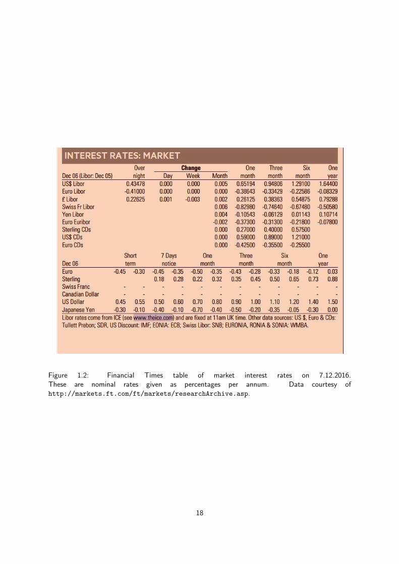
Figure 1.2: Financial Times table of market interest rates on 7.12.2016.These are nominal rates given as percentages per annum. Data courtesy ofhttp://markets.ft.com/ft/markets/researchArchive.asp.
18

1.2.3 Effective interest rates
The effective interest rate i is the total interest paid on one unit of money over one basic timeperiod. In other words, it is the interest rate converted from the nominal rate into the “equivalent”rate if compounding were carried out at the end of one basic time unit (rather than p-thly).
By equivalent, we mean the rate which gives the same accumulation after unit time. Now, theaccumulation factor for one time unit with interest at rate i per unit time is just [see Eq. (1.11)]
A(0, 1) = (1 + i). (1.18)
On the other hand, for compounding p-thly we have
A
(0,
1
p
)A
(1
p,
2
p
). . . A
(1− 1
p, 1
)=
(1 +
i(p)
p
)p. (1.19)
So, if the accumulations are the same, we require
1 + i =
(1 +
i(p)
p
)p. (1.20)
This is a very important relationship between the effective interest rate i and the nominal interest rateconverted p-thly i(p). You need to remember (1.20) or be able to reproduce quickly the argumentwhich gives it. Similarly, the rearranged formula
i(p) = p[(1 + i)1/p − 1], (1.21)
is often useful.Note:
• i = i(1).
• When the basic time period is 1 year, i is called the Effective Annual Rate (EAR) or theAnnual Equivalent Rate (AER).
• The AER is useful for comparing the annual cost of financial products with different periodsof compounding.
• Adverts for credit legally have to include the so-called Annual Percentage Rate (APR).3
This is defined as the effective annual rate of interest on a transaction obtained by taking intoaccount all the items entering the total charge for credit (i.e., including fees, etc.).
Example 1.2.2: AERYou wish to take out a loan and are offered two different deals. Bank A charges interest weekly at the nominalrate of 11% per annum. Bank B charges interest quarterly at the rate of 3% per quarter. Calculate the AERin each case and hence decide which bank offers the better deal.
SolutionBank A: Setting the basic time unit as 1 year, we have p = 52 since there are (approximately) 52 weeksin 1 year. We are given the nominal rate i(52) = 0.11 and therefore can use (1.20) to calculate the annualequivalent rate:
i =
(1 +
0.11
52
)52
− 1 (1.22)
= 0.1161 (to 4 d.p.). (1.23)
3Consumer Credit Act (1974)
19

Bank B: Here we are given that i(4)/4 = 0.03 (rate per quarter) and, using again (1.20),
i = (1 + 0.03)4 − 1 (1.24)
= 0.1255 (to 4 d.p.). (1.25)
Notice that in both cases the effective interest rate is slightly higher than the nominal interest rate (dueto the compounding of interest). Bank A offers a lower AER (approximately 11.61% p.a.) than Bank B(approximately 12.55% p.a.) so it is obviously the better choice for the loan.
An alternative strategy in problems which only involve one compounding time period (ratherthan a comparison) is to set the basic time unit equal to the compounding period. This is usuallyslightly quicker but, if you find it confusing, you may feel safer always setting unit time equal to oneyear (i.e., always measuring time in years).
Example 1.2.3: Quarterly interestIf interest is paid quarterly at the rate of 2% per quarter, what is the accumulation of an investment of £500after two years?
SolutionLet us set the basic time unit to be equal to one quarter. Then i(1) = i = 0.02 and (since there are 8 quartersin two years) we have
Accumulation = P × (1 + i)n (1.26)
= £500× (1 + 0.02)8 (1.27)
= £585.83 (to the nearest penny). (1.28)
Exercise 1.2.2: Quarterly interestConsider the same scenario as Example 1.2.3. Check that one gets the same answer by taking the basic timeunit to be equal to one year (so that i(4)/4 = 0.02); calculating i via (1.20) and then finding the accumulationfor n = 2.
Exercise 1.2.3: High APRFirst Premier Bank offers a credit card with an “APR of 79.9%” (p.a. is assumed here). If the interest iscompounded monthly and there are no other charges/fees (i.e., the APR is just the annual effective interestrate), determine how much a loan of $1000 increases to after just one month.[Answer: $1050.15 (to the nearest cent)]
Summary of 1.2
For general rates:
Accumulation factor for interest converted p-thly: A(t, t+ 1
p
)= 1 + i(p)(t)
p
Only for time-independent rates:
Relation between nom. and effect. interest rates: 1 + i =(
1 + i(p)
p
)p1.3 Force of interest
1.3.1 Time-dependent interest rates
So far we have assumed that interest rates are time-independent. In reality of course, interestrates usually vary due to changing economic circumstances. For time-dependent rates we define atime-dependent nominal rate i(p)(t), for transactions of term 1/p starting at time t, such that
A
(t, t+
1
p
)= 1 +
i(p)(t)
p(1.29)
20
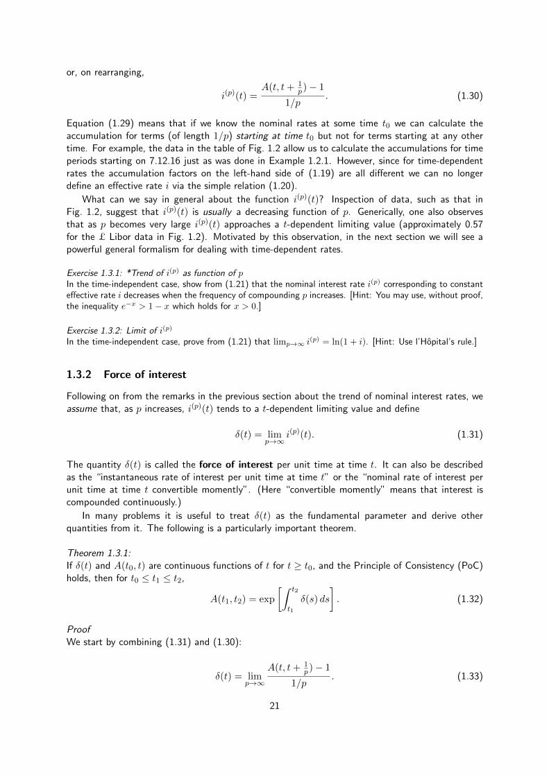
or, on rearranging,
i(p)(t) =A(t, t+ 1
p)− 1
1/p. (1.30)
Equation (1.29) means that if we know the nominal rates at some time t0 we can calculate theaccumulation for terms (of length 1/p) starting at time t0 but not for terms starting at any othertime. For example, the data in the table of Fig. 1.2 allow us to calculate the accumulations for timeperiods starting on 7.12.16 just as was done in Example 1.2.1. However, since for time-dependentrates the accumulation factors on the left-hand side of (1.19) are all different we can no longerdefine an effective rate i via the simple relation (1.20).
What can we say in general about the function i(p)(t)? Inspection of data, such as that inFig. 1.2, suggest that i(p)(t) is usually a decreasing function of p. Generically, one also observesthat as p becomes very large i(p)(t) approaches a t-dependent limiting value (approximately 0.57for the £ Libor data in Fig. 1.2). Motivated by this observation, in the next section we will see apowerful general formalism for dealing with time-dependent rates.
Exercise 1.3.1: *Trend of i(p) as function of pIn the time-independent case, show from (1.21) that the nominal interest rate i(p) corresponding to constanteffective rate i decreases when the frequency of compounding p increases. [Hint: You may use, without proof,the inequality e−x > 1− x which holds for x > 0.]
Exercise 1.3.2: Limit of i(p)
In the time-independent case, prove from (1.21) that limp→∞ i(p) = ln(1 + i). [Hint: Use l’Hopital’s rule.]
1.3.2 Force of interest
Following on from the remarks in the previous section about the trend of nominal interest rates, weassume that, as p increases, i(p)(t) tends to a t-dependent limiting value and define
δ(t) = limp→∞
i(p)(t). (1.31)
The quantity δ(t) is called the force of interest per unit time at time t. It can also be describedas the “instantaneous rate of interest per unit time at time t” or the “nominal rate of interest perunit time at time t convertible momently”. (Here “convertible momently” means that interest iscompounded continuously.)
In many problems it is useful to treat δ(t) as the fundamental parameter and derive otherquantities from it. The following is a particularly important theorem.
Theorem 1.3.1:If δ(t) and A(t0, t) are continuous functions of t for t ≥ t0, and the Principle of Consistency (PoC)holds, then for t0 ≤ t1 ≤ t2,
A(t1, t2) = exp
[∫ t2
t1
δ(s) ds
]. (1.32)
ProofWe start by combining (1.31) and (1.30):
δ(t) = limp→∞
A(t, t+ 1p)− 1
1/p. (1.33)
21

Now let h = 1/p, then
δ(t) = limh→0+
A(t, t+ h)− 1
h(1.34)
= limh→0+
A(t0, t)A(t, t+ h)−A(t0, t)
hA(t0, t)(1.35)
=1
A(t0, t)limh→0+
A(t0, t+ h)−A(t0, t)
h[using PoC]. (1.36)
Next, for convenience, we let F (t) = A(t0, t) (i.e., the value at t of one unit of money invested att0) and observe that (1.36) can be written as
δ(t) =1
F (t)limh→0+
F (t+ h)− F (t)
h. (1.37)
Recognising here the derivative4 of F we have
δ(t) =1
F (t)
dF (t)
dt(1.38)
=d
dt[lnF (t)] [chain rule]. (1.39)
Straightforward integration then yields∫ t
t0
δ(s) ds = lnF (t)− lnF (t0) (1.40)
= ln
(F (t)
F (t0)
), (1.41)
and upon inverting both sides and using F (t0) = A(t0, t0) = 1, we obtain
F (t) = A(t0, t) = exp
[∫ t
t0
δ(s) ds
], (1.42)
which proves the theorem, since t0, t are arbitrary.
Notice the appearance of the exponential function in this proof. In fact, the mathematicalconstant e was first “discovered” by Jacob Bernoulli during his 1683 studies of interest compoundedcontinuously [Ber89].
By substituting (1.32) in (1.30), we obtain i(p)(t) in terms of δ(t)
i(p)(t) =exp
[∫ t+1/pt δ(s) ds
]− 1
1/p, (1.43)
and the p = 1 case gives
i(t) = exp
[∫ t+1
tδ(s) ds
]− 1. (1.44)
Example 1.3.1: Force of interest and accumulation factorAssume that the force of interest varies with time and is given by δ(t) = a + b
t . Find the formula for theaccumulation of one unit of money from time t1 to time t2.
4Strictly the right-sided derivative.
22

SolutionBy Eq. (1.32),
A(t1, t2) = exp
[∫ t2
t1
(a+
b
s
)ds
](1.45)
= exp [(at2 + b ln t2)− (at1 + b ln t1)] (1.46)
= exp
[a(t2 − t1) + b ln
t2t1
](1.47)
= exp [a(t2 − t1)]
(t2t1
)b. (1.48)
Example 1.3.2: Force of interest and value of investmentAssume that the force of interest varies with time and is given by δ(t) = 0.02(1 + 1
1+t2 ) where t is measuredin years. Find the accumulation at time t = 1 of £1,000 invested at time t = 0.
SolutionAgain using Eq. (1.32),
Accumulation = C ×A(0, 1)
= £1000 exp
{∫ 1
0
0.02
(1 +
1
1 + s2
)ds
}= £1000 exp
{0.02 [s+ arctan s]
10
}= £1000 exp
{0.02
(1 +
π
4− 0− 0
)}= £1036.35 (to nearest penny).
Exercise 1.3.3: Force of interest and nominal interest ratesAssume that the force of interest varies as in Example 1.3.2. Use the relation (1.43) to find the value att = 0.5 of the nominal rate of interest per annum on transactions of term three months.[Answer: 3.45% p.a. (to 2 d.p.)]
Exercise 1.3.4: *Stoodley’s formulaStoodley’s formula is sometimes used to model gradually increasing or decreasing interest rates. It has theform
δ(t) = p+s
1 + rest(1.49)
where p, r and s are suitable parameters. Show that, if this formula holds, the accumulation of one unit ofmoney from time 0 to time t is given by
A(0, t) = exp[(p+ s)t]1 + r
1 + rest. (1.50)
1.3.3 Special case of constant force of interest
In some situations (including many exam questions) a constant, i.e., time-independent force ofinterest is assumed. For this special case δ(t) = δ for all t. Hence
A(t1, t2) = eδ×(t2−t1) (1.51)
which, in (1.43), leads straightforwardly to
i(p) = p(eδ/p − 1). (1.52)
The p = 1 case gives an important relationship between the effective rate i and the force of interest
i = eδ − 1 (1.53)
23

or, equivalently,δ = ln(1 + i). (1.54)
Combining this last equation with (1.51) we obtain that, for any n,
A(t0, t0 + n) = eδn (1.55)
= (1 + i)n. (1.56)
In other words, if interest on fractional time periods is paid at the nominal rate corresponding to thesame effective rate i, then the compound interest formula (1.11) [or (1.5)] holds also for non-integern!
Example 1.3.3: Double your money!If interest is compounded at an effective rate of 5% p.a., how long does it take an investment of £200 todouble in value?
SolutionWe take the basic time unit to be 1 year and set i = 0.05. Hence the doubling time is n years where nsatisfies the equation
400 = 200(1 + 0.05)n. (1.57)
This simplifies to2 = 1.05n, (1.58)
which is solved by taking logarithms of both sides to give
n =ln 2
ln 1.05= 14.21 (to 2 d.p.). (1.59)
So the investment doubles in approximately 14.2 years or, to the nearest month, 14 years and 2 months.[Note that the size of the original investment is irrelevant.]
Exercise 1.3.5: “Rule of 72”A rough rule-of-thumb dating back to at least the 15th Century [Pac94] is that, if interest is compounded atan effective rate of K% p.a., an investment takes approximately 72/K years to double. Check this againstthe exact doubling time for interest rates of 4%, 8% and 12%. You should find that for these values therelative error implied by the “Rule of 72” is less than 2%.
Example 1.3.4: Quadruple your money!Find the force of interest if an investment of 2000 Icelandic Krona quadruples in value in 10 years.
SolutionFrom Eq. (1.51), the force of interest δ must satisfy
2000eδ×10 = 8000 ⇔ e10δ = 4. (1.60)
Taking logarithms then yields
δ =1
10ln 4 = 0.1386 p.a. (to 4 d.p.). (1.61)
Exercise 1.3.6: Limit of i(p)
Starting from Eq. (1.52), show that limp→∞ i(p) = δ, i.e., the special case of (1.31) for time-independentrates. [Hint: Compare Exercise 1.3.2.]
Exercise 1.3.7: *Approximate expressions for δ and i in terms of i(p) when p is largeStarting from Eqs. (1.54) and (1.20) use Taylor’s expansion of ln(1 + x), |x| < 1 (Calculus I) to obtain:
δ = i(p) − [i(p)]2
2p+ ε, where |ε| ≤ [i(p)]3
3p2(1.62)
= i(p) − [i(p)]2
2p+
[i(p)]3
3p2+ ε, where |ε| ≤ [i(p)]4
4p3. (1.63)
24
Formula (1.62) can be used to give another proof of the fact that the force of interest is the nominal rate ofinterest compounded instantly. Try to find this proof.
Summary of 1.3
Force of interest: δ(t) = limp→∞
i(p)(t) = limh→0+
A(t,t+h)−1h
Accumulation at t2 of a unit invest. at t1: A(t1, t2) = exp[ ∫ t2
t1δ(s) ds
]Constant force of interest δ: eδ = 1 + i =
[1 + i(p)
p
]p1.4 Rates of discount
Let us consider the case of a time-varying force of interest δ(t) (i.e., for now we do not assume aconstant force of interest).
Assume that interest is compounded p-thly and recall, from Section 1.2, that the interest foruse of one unit of money over one subperiod of time of length 1/p starting at time t is i(p)(t)/p.Note that it is assumed that this interest is paid in arrears at the end of the subperiod, i.e., at timet+ 1/p. So, restating our previous definition, we have:
i(p)(t) is the rate per unit time and per unit capital at which interest for use of money over timeperiod [t, t+ 1/p] is paid in arrears (i.e., at t+ 1/p).
However, in some circumstances one might pay for use of money in advance at the start ofthe subperiod. The amount of the equivalent payment, for use of one unit of money, is denoted byd(p)(t)/p where d(p)(t) is called the nominal rate of discount compounded p-thly (or convertiblep-thly) and defined such that:
d(p)(t) is the rate per unit time and per unit capital at which interest for use of money over timeperiod [t, t+ 1/p] is paid in advance (i.e., at t).
When p = 1 we drop the subscript, i.e., d(t) is the rate at which interest for use of money over unittime period is paid in advance.
We have defined A(t1, t2) as the accumulation at time t2 of one unit of money invested at timet1. Analogously, we now define D(t1, t2) as the value of an investment at time t1 which gives areturn of one unit of money at time t2. You should be able to convince yourself easily that
D(t1, t2) =1
A(t1, t2)(1.64)
= exp
[−∫ t2
t1
δ(s) ds
]. (1.65)
Now, when we borrow one unit of money for use over one subperiod and pay interest in advance,we actually receive 1− d(p)(t)/p at time t and repay 1 at time t+ 1/p. Hence it follows that
D
(t, t+
1
p
)= 1− d(p)(t)
p. (1.66)
Exercise 1.4.1: Rates of discount for differing subperiodsBy working backwards through one time unit (and assuming the Principle of Consistency) show that
1− d(0) =
[1−
d(4)( 34 )
4
][1−
d(2)( 14 )
2
] [1− d(4)(0)
4
]. (1.67)
25

1.4.1 Relation between nominal rates of discount and interest
The nominal rates of interest and discount are related since payment of d(p)(t)/p at time t isequivalent to payment of i(p)(t)/p at time t + 1/p. Or, in other words, an investment of d(p)(t)/pat time t gives a return of i(p)(t)/p at time t+ 1/p. Therefore
A
(t, t+
1
p
)d(p)(t)
p=i(p)(t)
p. (1.68)
The validity of this equation can be easily seen as follows. Imagine that we have instead
A
(t, t+
1
p
)d(p)(t)
p>i(p)(t)
p. (1.69)
Then it would be possible to obtain a risk-free profit: 1. Borrow 1 unit of money at time t with
interest paid in arrears. For this you need to pay i(p)(t)p at time t + 1/p. 2. Loan this money to
another person with interest paid in advance. You receive d(p)(t)p at time t. But now you can invest
this money in a bank account over the time period [t, t + 1/p], and if Eq. (1.69) holds you can
pay i(p)(t)p and still make a profit. A similar reasoning can be made for < in Eq. (1.69) switching
borrowing and loaning. In a financial market, such a risk-free profit is not possible, therefore theequality has to hold in Eq. (1.69).
Using Eq. (1.29), we obtain
d(p)(t)
p=
i(p)(t)p
1 + i(p)(t)p
(1.70)
Notice that this equation implies that the nominal rate of discount compounded p-thly is alwayssmaller than the nominal rate of interest compounded p-thly. Trivial rearrangement of (1.70) gives
1
d(p)(t)=
1
i(p)(t)+
1
p(1.71)
which may be easier to remember. From this form of the relation it follows obviously that
limp→∞
d(p)(t) = limp→∞
i(p)(t) = δ(t) (1.72)
which is consistent with the intuition that for compounding continuously it makes no differencewhether we pay interest in advance or in arrears.
Exercise 1.4.2: Relation between nominal rates of discount and interestGive an alternative derivation of (1.70) starting from (1.64).
Special case of constant force of interest
For the remainder of Section 1.4 we specialize again to the practically important case of constantforce of interest. By substituting i(p)(t) = i(p) = p(eδ/p − 1) [see (1.52)] in (1.70) we obtain thatd(p)(t) = d(p) where
d(p) = peδ/p − 1
1 + eδ/p − 1(1.73)
= p(1− e−δ/p). (1.74)
For p = 1 we have
d =i
1 + i= 1− e−δ, (1.75)
where d is called the effective rate of discount (or, if unit time is one year, the annual rate ofdiscount).
26

Exercise 1.4.3: Relation between d and iInterpret the first equality in (1.75) in words.
Relation between nominal and effective rates of discount
There are many ways to derive a relation between d and d(p). One possibility is to start from (1.74)which can be rearranged to give
e−δ/p = 1− d(p)
p(1.76)
which leads to
e−δ =
(1− d(p)
p
)p(1.77)
and, using (1.75),
1− d =
(1− d(p)
p
)p. (1.78)
Equation (1.78) should be compared with (1.20).
Example 1.4.1: Interest and discountSuppose interest is paid at an AER of 3% p.a.. You take out a loan of £1,000 for 6 months. How muchinterest should you pay if the interest is paid in arrears? And how much if the interest is paid in advance?
SolutionTake the basic time unit equal to 1 year, then i = 0.03 and
i(2)
2=
2[(1 + i)1/2 − 1]
2[using (1.21)] (1.79)
= 0.14889 (to 5 d.p.) (1.80)
Now
Interest paid in arrears = £1000× i(2)
2(1.81)
= £14.89 (to nearest penny), (1.82)
and
Interest paid in advance = £1000× d(2)
2(1.83)
= £1000×i(2)
2
1 + i(2)
2
[using (1.70)] (1.84)
= £14.67 (to nearest penny). (1.85)
Noticee that, as we expect, the interest paid in advance is slightly less than the interest paid in arrears; indeed£14.67 = £14.89/(1 + i)1/2.
Exercise 1.4.4: Key relationshipsLook back through Sections 1.2–1.4 and combine equations to show that, for constant force of interest,[
1 +i(p)
p
]p= 1 + i = eδ =
1
1− d=
1[1− d(p)
p
]p . (1.86)
If you remember this series of equalities then, given any one of i(p), i, δ, d(p) or d, you can find any of theothers by simple rearrangement.
27

Example 1.4.2: Conversion from d to i(12)
Given that d = 0.0625, find i(12).
SolutionFrom Eq. (1.86), we have [
1 +i(p)
p
]p=
1
1− d(1.87)
which can be rearranged to yield
i(p) = p
[1
(1− d)1/p− 1
]. (1.88)
Hence, for d = 0.0625,
i(12) = 12[(1− 0.0625)−1/12 − 1
](1.89)
= 0.0647 (to 4 d.p.). (1.90)
[Note that it should not be necessary to memorize (1.88), or to calculate intermediate quantities such as i orδ.]
Exercise 1.4.5: *Inequalities for ratesShow that
d = d(1) < d(2) < d(3) < . . . < d(p) < . . . < δ < . . . < i(p) < . . . < i(3) < i(2) < i(1) = i (1.91)
[Hint: Compare Exercise 1.3.1.]
Summary of 1.4
For general force of interest:
Discounted value at t1 of a unit invst. at time t2: D(t1, t2) = exp[−∫ t2t1δ(s)ds
]When interest is converted p-thly: D
(t, t+ 1
p
)= 1− d(p)(t)
p
Relation between nom. discount and interest rates: 1d(p)(t)
= 1i(p)(t)
+ 1p
Only for constant force of interest:
Relation between nom. and eff. discount rates: 1− d =[1− d(p)
p
]p1.5 Discounting Cash Flows or Present Values
From Section 1.3, we know that the value at time t2 of an investment of C at time t1 is C ×A(t1, t2) = C exp
[∫ t2t1δ(s)ds
]. On the other hand, from Section 1.4, the value at time t1 of an
investment of C at time t2 is C × D(t1, t2) = C exp[−∫ t2t1δ(s)ds
]. This enables us to find the
value at any time of an investment whose value we know at any other time. In this section, we willuse this approach to compare the values of cash flows restricting the analysis to the case of constantforce of interest (with the exception of Exercises 1.8.1 and 1.8.2).
For constant force of interest we have,
A(t1, t2) = (1 + i)(t2−t1) and D(t1, t2) = (1 + i)−(t2−t1). (1.92)
For brevity of writing we now define the discounting factor
v =1
1 + i= 1− d = e−δ (1.93)
28

and note that with this notation A(t, 0) = D(0, t) = vt.
The quantity Cvt is called the (discounted) present value of C due at time t. We will abbreviatethis to P.V..
In practice this means that you must remember the following simple rules. Suppose we investan amount of C at some time. Then...
• ...to find the value of the investment t years later you multiply C by (1 + i)t;
• ...to find the value of the investment t years earlier you multiply C by vt .
We will now use these rules to evaluate and compare the values of cash flows. Here a cash flowmeans a series of payments. When considering cash flows, it is important to recognise the timing ofeach cash flow; is the cashflow at the beginning of the month or the end of the month or, perhaps,in the middle of the month?
1.5.1 Discrete cash flows
This is the most common case. Consider payments of c1, c2, . . . cn due at times t1, t2, . . . , tn in thefuture. The present value 5 (i.e. at time t = 0) of such a cash flow is given by
P.V. of discrete cash flow = c1vt1 + c2v
t2 + . . .+ cnvtn =
n∑j=1
cjvtj . (1.94)
In many problems we are interested in comparing cash inflow and cash outflow. To compare twocash flows we must look at their values at the same time; it’s usually best to choose the present timeand to compare P.V.s. Two cash flows are equivalent if they have the same P.V.. If the presentvalue of cash inflows is equal to the present value of cash outflows at a particular rate of interest,it means that the outgoing cash flows when invested with interest will generate the incoming cashflows. Equality of inflows and outflows is expressed by the so-called equation of value
P.V. of outgoing cash flows = P.V. of incoming cash flows. (1.95)
The equation of value can be expressed at any point of time. It brings together three quantities:amount(s), time(s) and rate of interest. If the others are known, an unknown quantity from this listcan be determined by the equation of value.
Example 1.5.1: Equation of valueA borrower is under an obligation to repay a bank £6,280 in four years’ time, £8,460 in seven years’ time and£7,350 in thirteen years’ time. As part of a review of his future commitments the borrower now offers eitherof the following:
• to discharge his liability for these three debts by making an appropriate single payment five years fromnow (offer A);
• to repay the total amount owed (i.e., £22,090) in a single payment at an appropriate time (offer B).
On the basis of a constant rate of interest 8% per annum effectively, find the appropriate single paymentif offer A is accepted by the bank, and the appropriate time to repay the entire indebtedness if offer B isaccepted.
5Many authors use the terminology Net Present Value, abbreviated to NPV, to denote the present value of a cashflow.
29
SolutionWe take 1 year as the basic time unit so that i = 0.08 and
v =1
1 + i=
1
1.08. (1.96)
Offer A:We need to find £C such that the following two cash flows are equivalent.
Out: £C at t = 5,
In: £6280 at t = 4, £8460 at t = 7, and £7350 at t = 13.
The equation of value expressed at the present time, t = 0, is
Cv5 = 6280v4 + 8460v7 + 7350v13 (1.97)
but in fact the equation of value expressed at t = 4 has a simpler form
Cv = 6280 + 8460v3 + 7350v9. (1.98)
This is easily solved for C
C =6280 + 8460v3 + 7350v9
v(1.99)
= 18006.46 (to 2 d.p.). (1.100)
So the borrower should make a single payment of £18,006.46 (to the nearest penny).
Offer B:We need to find tp such that the following two cash flows are equivalent.
Out: £22090 at t = tp,
In: £6280 at t = 4, £8460 at t = 7, and £7350 at t = 13.
In this case, the equation of value expressed at the present time, t = 0, is
22090vtp = 6280v4 + 8460v7 + 7350v13, (1.101)
and solving for tp yields
tp =ln 6280v4+8460v7+7350v13
22090
ln v(1.102)
= 7.66 (to 2 d.p.). (1.103)
So the borrower should make the payment after approximately 7 years and 8 months.
Summary of 1.5
Discounting factor: v = 11+i = 1− d
Discounted present value of C due in time t: Cvt
Equation of value: P.V. of outflow = P.V. of inflow
30
1.6 Annuities-certain: introduction
An annuity is a series of payments made at regular time intervals. We restrict ourselves here mainlyto level annuities where the payments are all equal.
There are two sorts of annuities: annuities-certain and life annuities. For an annuity certainthe number of payments is certain and specified in the contract. In contrast, the payments maydepend on the survival of one or more human lives, then we say life annuity. In that case, the numberof payments is uncertain. For example, pensions are life annuities.
In this section we look at annuities-certain; life annuities will be considered later. We willderive the P.V.s, for annuities-certain where one unit of money is paid per unit time. Obviously forannuities where payment is C units of money per unit time, the P.V. is obtained by multiplying thecorresponding expression by C.
The main mathematical result we will need is the well-known formula for the sum of a geometricprogression:
N−1∑j=0
qj = 1 + q + q2 + . . .+ qN−1 =1− qN
1− q, for any q 6= 1. (1.104)
1.6.1 Immediate annuity
Consider n payments of one unit of money to be made at intervals of one unit of time with the firstpayment due one unit of time from now (i.e., the first payment is at time 1 and the last at time n).This situation is known as an immediate annuity, the symbol for its present value is an and
an = v + v2 + . . .+ vn = v1− vn
1− v. (1.105)
OR
an =1− vn
imultiplying numerator and denominator by (1 + i) and simplifying. (1.106)
Note that the payments are made in arrears, i.e., at the end of each time period and that here, asthroughout this section, we assume a constant (and strictly positive) force of interest. In actuarialnotation, a subscript enclosed in a right angle always indicates the (fixed) term of the given financialobject.
1.6.2 Annuity-due
Now consider the same series of payments as in the previous paragraph but with payments made inadvance, i.e., at the beginning of each time period (so that the first payment is at time 0 and thelast at n − 1). This situation is known as an annuity-due, the symbol for its present value is anand
an = 1 + v + . . .+ vn−1 =1− vn
1− v. (1.107)
Notice that an = van , and an = 1 + an−1 . An immediate annuity is also known as an annuitypaid in arrears.
Exercise 1.6.1: Relations between annuitiesInterpret the equalities in the last sentence in words.
Example 1.6.1: Annuity-dueA loan of £300,000 is to be repaid by ten equal annual instalments, the first is due now. Find the annualpayment if the interest on the loan is charged at the AER of 12.99% p.a..
31

SolutionLet £C be the annual payment. Take 1 year as the unit time. Then i = 0.1299 and the discounting factor isgiven by
v =1
1 + i=
1
1.1299. (1.108)
Now the loan is to be repaid by an annuity-due payable annually at rate £C per annum. The presentvalue of the repayments is thus Ca10 and equating P.V.s we obtain the equation of value:
300000 = Ca10 . (1.109)
Hence
C =300000
a10=
300000(1− v)
1− v10= 48911.2067 (to 4 d.p.). (1.110)
So the annual repayment is £48, 911.21 (to the nearest penny).Note, if there is likely to be any confusion about the value of i (and especially for questions involving
more than one interest rate), it is wise to state explicitly the interest rate implicit in a given function. Forexample, one could write (1.109) in the form
300000 = Ca10 at 12.99%. (1.111)
An alternative notation is to use a vertical bar and an @ symbol. For example
C =300000(1− v)
1− v10
∣∣∣∣@i=0.1299
. (1.112)
An annuity-due is also known as an annuity paid in advance.
1.6.3 Perpetuities
Notice that an and an are monotone increasing functions of n. Considering the limit of n → ∞corresponds to payments being made “in perpetuity”. One finds
a∞ = limn→∞
an =v
1− v=
1
i, (1.113)
and
a∞ = limn→∞
an =1
1− v=
1
d, (1.114)
which give the present values of an immediate perpetuity and a perpetuity-due respectively.The income from equity share or from a property investment will often be valued ”in perpetuity”
using the approach above.
1.6.4 Deferred annuities
Suppose a series of n unit payments starts at time m+ 1, the last one due at time m+n. This maybe considered as an immediate annuity deferred m time periods. The symbol for the presentvalue is m|an and
m|an = vm+1 + . . .+ vm+n = vman (1.115)
Similarly one can define an annuity-due deferred m time periods whose present value is m|an =vman .
Exercise 1.6.2: More relations between annuitiesShow that m|an = am+n − am and m|an = am+n − am .
Exercise 1.6.3: Deferred annuityJohn Doe wishes to purchase a deferred annuity of £10,000 per annum paid out for ten years. Payments aremade annually, the first payment being due in two years’ time. What is the present value of the annuity ifthe annual effective interest rate stays at 10% over this period?[Answer: £55,859.70 (to nearest penny)]
32

1.6.5 Increasing annuities
Annuities where the payments are not equal are called varying annuities. In particular, an annuitywhich pays k units of money at the end of the kth time period (i.e., 1 unit of money at the end ofthe first time period, 2 units of money at the end of the second time period, and so on, up to nunits of money at the end of the nth time period) is called an increasing immediate annuity. Itspresent value is denoted (Ia)n and it can be shown that
(Ia)n = v + 2v2 + 3v3 + . . .+ nvn =an − nvn
i. (1.116)
Similarly, an annuity paying k units of money at the beginning of the kth time period for n timeperiods is an increasing annuity-due and has present value
(Ia)n = 1 + 2v + 3v2 + 3v3 + . . .+ nvn−1 = (1 + i)(Ia)n . (1.117)
Summary of 1.6
P.V. of annuity-due: an = 1−vn1−v
P.V. of immediate-annuity: an = vanP.V.s of deferred annuities: m|an = vman , m|an = vman
1.7 Annuities-certain: more variations
1.7.1 Annuities payable p-thly
Consider an annuity of one unit of money per unit time payable over n units of time in instalmentsof 1/p at p-thly intervals. In the case where the payments are made in arrears (so that the first one isdue one p-thly interval from now at time 1/p), we have an immediate annuity payable p-thly. Its
present value is denoted by the symbol a(p)n . By summing the present values of the n× p individual
payments we obtain
a(p)n =
1
pv1/p +
1
pv2/p + . . .+
1
pvnp/p (1.118)
=1
pv1/p
(1 + v1/p + . . .+ v(np−1)/p
)(1.119)
=1
pv1/p
1− vn
1− v1/p[using (1.104) with q = v1/p]. (1.120)
Obviously the p = 1 case reduces to the present value of an “ordinary” immediate annuity paidannually, as given by (1.105).
Example 1.7.1: Mobile phone contractSuppose you sign a mobile phone contract agreeing to pay £15 at the end of each month for the next twoyears. Assuming a constant AER of 2% p.a., what is the present value of the whole series of payments? (Inother words, what lump sum of money would you need to put in the bank now to cover all the future monthlypayments?)
SolutionTake 1 year as the basic time unit, then i = 0.02 and
v =1
1 + i=
1
1.02. (1.121)
33
The payments form an immediate annuity payable monthly (p = 12) at the rate of £180 per year. Hence therequired P.V. is given by
P.V. = £180× a(12)2
(1.122)
= £180× 1
12v1/12
1− v2
1− v1/12(1.123)
= £352.67 (to the nearest penny). (1.124)
As expected, this is slightly less than £360 because of the interest paid over the two years.
Exercise 1.7.1: *Mobile phone contract (alternative solution)An alternative solution for Example 1.7.1 is to choose 1 month as the basic time unit. Then i (the effectiveinterest rate per time unit) is given by (1 + 0.02)1/12 − 1 = 0.00165158 (to 8 d.p.) and
v =1
1 + i≈ 1
1.00165158. (1.125)
With 1 month as the basic time unit and v as given by (1.125) the required P.V. is
P.V. = £15× a24 . (1.126)
Check that this gives the same answer as (1.124), and that you understand why. [To avoid numerical errors,be careful not to round up the value for v given in (1.125).]
Now consider the same situation (an annuity of one unit of money per unit time payable p-thlyover n time units) but with the first payment due at time 0, i.e., payment in advance. In this casewe have an annuity-due payable p-thly whose P.V. is given by
a(p)n =
1
p
(1 + v1/p + . . .+ v(np−1)/p
)=
1
p
1− vn
1− v1/p. (1.127)
Analogously to the discussion at the end of Section 1.6 one can also consider annuities payable
p-thly deferred by m time units. It should be obvious that their P.V.s are given by m|a(p)n = vma(p)n
and m|a(p)n = vma(p)n . In particular, note that 1/p|a
(p)n = a
(p)n . (Why?)
One can also derive alternative formulae for the P.V.s of annuities payable p-thly which illustratethe relation to nominal rates of interest/discount. For example, start from (1.120) and use thatv1/p = e−δ/p [follows from Eq. (1.93)] to obtain
a(p)n =
1
pe−δ/p
1− vn
1− e−δ/p(1.128)
=1− vn
p(eδ/p − 1)(1.129)
=1− vn
i(p)[using (1.52)]. (1.130)
Exercise 1.7.2: Alternative formula for a(p)n
Show that
a(p)n =
1− vn
d(p). (1.131)
1.7.2 Annuities payable continuously
If payments are frequent they can be approximated by the theoretical construction of a continuousannuity as we discuss below.
34

Suppose payments are made continuously over n units of time at the rate of one unit of moneyper unit time. The present value of this payment stream is denoted by an . To evaluate it, we firstimagining partitioning each time unit into small subintervals of length 1/p. Then
an =
np∑k=1
{P.V. of payment in between t =
k − 1
pand t =
k
p
}(1.132)
If p is large, so that each subinterval is small, then we can approximate the continuous paymentbetween t = (k − 1)/p and t = k/p as a discrete payment of 1/p at t = k/p. Hence, for large p,we have,
an ≈np∑k=1
1
pvk/p = a
(p)n . (1.133)
The approximate relation an ≈ a(p)n becomes exact in the limit p → ∞ which gives one way of
calculating an :
an = limp→∞
a(p)n (1.134)
= limp→∞
1− vn
i(p)[using (1.130)] (1.135)
=1− vn
δ. [using the time indep. form of (1.31)]. (1.136)
Exercise 1.7.3: p→∞ of annuity-due
Show that taking limp→∞ a(p)n gives the same result as (1.136), and explain why (in words).
Example 1.7.2: Deferred perpetuitiesThe AER is 8% p.a.. Find the present value of a deferred annuity of £13,000 per year paid in perpetuity inthe following cases:(i) Payments are made monthly with the first payment in 6 months’ time.(ii) Payments are made continuously in time starting in 6 months’ time.
SolutionWe take the basic time unit to be one year so that i = 0.08 and
v =1
1.08. (1.137)
(i) Here we have a perpetuity-due payable 12-thly and deferred by half a time unit (6 months). Rememberthat the symbol a (with associated labels) always refers to an annuity of one unit of money per unit time sothat here the required P.V. (in pounds) is expressed as:
P.V. = 13000× 1/2|a(12)∞ (1.138)
= 13000v1/2 limn→∞
a(12)n (1.139)
= 13000v1/2 limn→∞
1
12
1− vn
1− v1/12(1.140)
=13000
12
v1/2
1− v1/12(1.141)
= 163061.8827 (to 4 d.p.). (1.142)
So the present value of the specified perpetuity is £163,061.88 (to the nearest penny).6
6Note that if you’ve specified that you’re working in pounds (as we did here above (1.138)), then you don’t needto include the £ sign in the intermediate calculations but you should always give units in the final answer.
35

(ii) Here we have a perpetuity payable continuously, again deferred by half a time unit (6 months). Therequired P.V. (in pounds) is given by
P.V. = 13000× 1/2|a∞ (1.143)
= 13000v1/2 limn→∞
an (1.144)
= 13000v1/2 limn→∞
1− vn
δ(1.145)
= 13000v1/2
δ(1.146)
= 13000v1/2
ln(1 + i)(1.147)
= 162540.1066 (to 4 d.p.). (1.148)
So the present value of the specified perpetuity is £162,540.11 (to the nearest penny).
1.7.3 Accumulated values
Until now we have discussed how to calculate the present value of an annuity at time 0. Supposethat instead, we are interested in the accumulated value (accumulation) at the end of the series ofpayments, i.e., at time n if it’s an annuity of term n. In fact, this is very simple to obtain from thecorresponding present value but does involve the introduction of yet another symbol...
To be specific consider an immediate annuity (of one unit of money per unit time) payablep-thly over n time units. The accumulated value at time n, after the last payment has been made,
is usually denoted by s(p)n . From the discussion at the beginning of Section 1.5 it follows that
s(p)n = (1 + i)na
(p)n , or a
(p)n = vns
(p)n . (1.149)
Of course, there is a similar relation between the present and accumulated values of an annuity-due,
s(p)n = (1 + i)na
(p)n , or a
(p)n = vns
(p)n , (1.150)
and between the present and accumulated values of a continuous annuity,
sn = (1 + i)nan , or an = vnsn , (1.151)
Don’t worry too much about remembering the s symbol. It’s much more important that youunderstand that the accumulated value of an annuity-certain, of term n, is always given by theassociated present value multiplied by (1 + i)n.
Summary of 1.7
P.V. of annuity-due payable p-thly: a(p)n = 1
p
[1−vn1−v1/p
]P.V. of immediate-annuity payable p-thly: a
(p)n = v1/pa
(p)n
P.V. of continuous annuity: an = 1−vnδ
Accumulated values of annuities: s(p)n = (1 + i)na
(p)n , s
(p)n = (1 + i)na
(p)n
36

1.8 Continuous cash flows (not examinable)
Continuously payable cash flows are also known as payment streams. They are a theoretical conceptbut sometimes a useful approximation, e.g., payments made daily or weekly can be consideredpractically continuous if we are interested in times on a scale of years. The cash flow can consist ofboth incoming and outgoing transactions and so it’s possible that the net cash flow ρ(t) is negative.
We define ρ(t) as the rate (per unit time) at which payment is made at time t, i.e.,
ρ(t) = limh→0+
{1
h× (amount paid over [t, t+ h])}. (1.152)
The present value of such a continuous payment stream over time interval [t1, t2] in the future isthen given by
P.V. of continuous cash flow =
∫ t2
t1
vtρ(t) dt. (1.153)
The integration in the case where ρ(t) = ρ is particularly simple:
P.V. of constant continuous cash flow =
∫ t2
t1
vtρ dt (1.154)
=
∫ t2
t1
e−δtρ dt (1.155)
=[−ρδe−δt
]t2t1
(1.156)
=ρ
δ(e−δt1 − e−δt2). (1.157)
Example 1.8.1: Linear cash flowConsider a continuous cash flow having a linear payment density of the form
ρ(t) =
{at for t1 ≤ t ≤ t20 otherwise
(1.158)
with a a time-independent constant. Find the present value of this cash flow at time t = 0.
Solution
P.V. =
∫ t2
t1
vtat dt (1.159)
= a
∫ t2
t1
e−δtt dt (1.160)
= a
{[t
(−1
δe−δt
)]t2t1
−∫ t2
t1
(−1
δe−δt
)dt
}[integration by parts] (1.161)
= a
{[−δte−δt − e−δt
δ2
]t2t1
}(1.162)
=a{(1 + δt1)e−δt1 − (1 + δt2)e−δt2}
δ2. (1.163)
Exercise 1.8.1: *Another derivation of the P.V. of a continuous annuityConsider a continuous cash flow between t1 = 0 and t2 = n with rate ρ = 1 per unit time. The present valueof such a payment stream is given by the integral in (1.154). Show that this gives the same expression foran as in (1.136).
37
t=0 t= 1p t= 2
p ... t= p−1p t=1 Time, t
(1) d
(2) d(p)
pd(p)
pd(p)
p . . . d(p)
p
(3) i(p)
pi(p)
p . . . i(p)
pi(p)
p Payments
(4) i
(5) ←− Continuous payment at rate δ −→
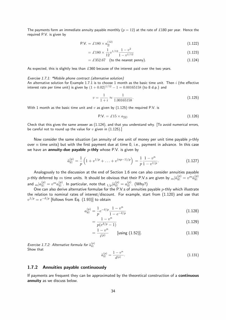
Table 1.1: Five equivalent ways of paying interest on 1 unit of money over [0, 1].
1.8.1 Continuous cash flow with variable force of interest
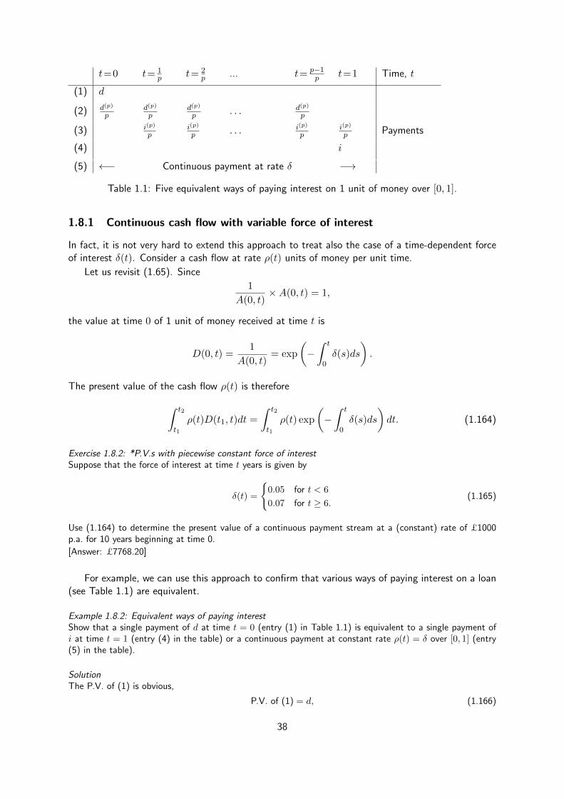
In fact, it is not very hard to extend this approach to treat also the case of a time-dependent forceof interest δ(t). Consider a cash flow at rate ρ(t) units of money per unit time.
Let us revisit (1.65). Since
1
A(0, t)×A(0, t) = 1,
the value at time 0 of 1 unit of money received at time t is
D(0, t) =1
A(0, t)= exp
(−∫ t
0δ(s)ds
).
The present value of the cash flow ρ(t) is therefore∫ t2
t1
ρ(t)D(t1, t)dt =
∫ t2
t1
ρ(t) exp
(−∫ t
0δ(s)ds
)dt. (1.164)
Exercise 1.8.2: *P.V.s with piecewise constant force of interestSuppose that the force of interest at time t years is given by
δ(t) =
{0.05 for t < 6
0.07 for t ≥ 6.(1.165)
Use (1.164) to determine the present value of a continuous payment stream at a (constant) rate of £1000p.a. for 10 years beginning at time 0.
[Answer: £7768.20]
For example, we can use this approach to confirm that various ways of paying interest on a loan(see Table 1.1) are equivalent.
Example 1.8.2: Equivalent ways of paying interestShow that a single payment of d at time t = 0 (entry (1) in Table 1.1) is equivalent to a single payment ofi at time t = 1 (entry (4) in the table) or a continuous payment at constant rate ρ(t) = δ over [0, 1] (entry(5) in the table).
SolutionThe P.V. of (1) is obvious,
P.V. of (1) = d, (1.166)
38

and the other two are easily calculated
P.V. of (4) = iv (1.167)
= d [using (1.75)], (1.168)
P.V. of (5) =δ
δ(1− e−δ) [using (1.157)] (1.169)
= d [again using (1.75)]. (1.170)
The three cash flows have the same P.V., therefore they are all equivalent.
Exercise 1.8.3: Equivalent ways of paying interestShow that entries (2) and (3) in Table 1.1 are also equivalent to the three methods of paying interest consideredin Example 1.8.2. [Hint: You will need to sum a geometric progression.]
Example 1.8.3: Increasing annuity payable continuouslyConsider a continuous annuity which has a constant rate of payment k (per unit time) throughout the kthtime period. The present value of such an annuity is denoted by (Ia)n ; show that it is given by
(Ia)n =an − nvn
δ. (1.171)
SolutionObviously the total P.V. can be expressed as a sum over the P.V.s for each time period so we have
(Ia)n =
n∑k=1
(∫ k
k−1kvt dt
)(1.172)
=
n∑k=1
k
δ
(e−δ(k−1) − e−δk
)[using (1.157)] (1.173)
=
∑n−1j=0 (j + 1)e−δj −
∑nk=1 ke
−δk
δ[using j = k − 1] (1.174)
=
∑n−1k=0(k + 1)e−δk −
∑n−1k=0 ke
−δk − ne−δn
δ[relabelling j as k] (1.175)
=
∑n−1k=0 e
−δk − ne−δn
δ(1.176)
=
∑n−1k=0 v
k − nvn
δ(1.177)
=an − nvn
δ. (1.178)
Exercise 1.8.4: *Spot the difference!Another form of increasing continuous annuity has a rate of payment t at time t (i.e., a linear paymentdensity). The present value of this variation is denoted by (I a)n ; show that it is given by
(I a)n =an − nvn
δ. (1.179)
[Hint: Consider Example 1.8.1]
Accumulated value of a continuous cash flow
Suppose that for a continuous time cash flow payments begin at time t1 and end at time t2 andassume time-dependent force of interest δ(t). The accumulated value of a continuous time cashflow ρ(t) at the time t2 is∫ t2
t1
ρ(t)A(t, t2)dt =
∫ t2
t1
ρ(t) exp
(∫ t2
tδ(s)ds
)dt.
39
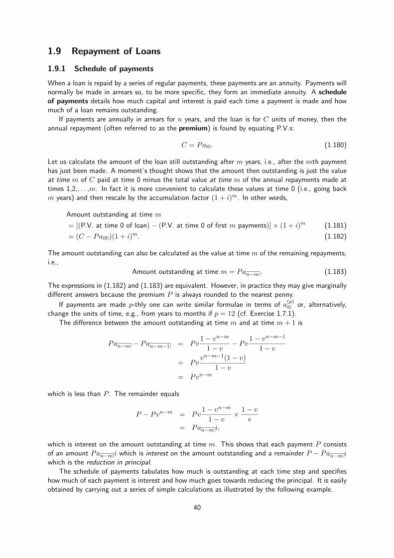
1.9 Repayment of Loans
1.9.1 Schedule of payments
When a loan is repaid by a series of regular payments, these payments are an annuity. Payments willnormally be made in arrears so, to be more specific, they form an immediate annuity. A scheduleof payments details how much capital and interest is paid each time a payment is made and howmuch of a loan remains outstanding.
If payments are annually in arrears for n years, and the loan is for C units of money, then theannual repayment (often referred to as the premium) is found by equating P.V.s:
C = Pan . (1.180)
Let us calculate the amount of the loan still outstanding after m years, i.e., after the mth paymenthas just been made. A moment’s thought shows that the amount then outstanding is just the valueat time m of C paid at time 0 minus the total value at time m of the annual repayments made attimes 1,2,. . . ,m. In fact it is more convenient to calculate these values at time 0 (i.e., going backm years) and then rescale by the accumulation factor (1 + i)m. In other words,
Amount outstanding at time m
= [(P.V. at time 0 of loan)− (P.V. at time 0 of first m payments)]× (1 + i)m (1.181)
= (C − Pam )(1 + i)m. (1.182)
The amount outstanding can also be calculated as the value at time m of the remaining repayments,i.e.,
Amount outstanding at time m = Pan−m . (1.183)
The expressions in (1.182) and (1.183) are equivalent. However, in practice they may give marginallydifferent answers because the premium P is always rounded to the nearest penny.
If payments are made p-thly one can write similar formulae in terms of a(p)n or, alternatively,
change the units of time, e.g., from years to months if p = 12 (cf. Exercise 1.7.1).
The difference between the amount outstanding at time m and at time m+ 1 is
Pan−m − Pan−m−1 = Pv1− vn−m
1− v− Pv1− vn−m−1
1− v
= Pvvn−m−1(1− v)
1− v= Pvn−m
which is less than P . The remainder equals
P − Pvn−m = Pv1− vn−m
1− v× 1− v
v= Pan−m i,
which is interest on the amount outstanding at time m. This shows that each payment P consistsof an amount Pan−m i which is interest on the amount outstanding and a remainder P − Pan−m iwhich is the reduction in principal.
The schedule of payments tabulates how much is outstanding at each time step and specifieshow much of each payment is interest and how much goes towards reducing the principal. It is easilyobtained by carrying out a series of simple calculations as illustrated by the following example.
40

Example 1.9.1: Schedule of paymentsDetermine the schedule of payments on a loan of £10,000 to be repaid by equal annual payments, at effectiveinterest rate 10% p.a., over five years with the first payment due in one year from now.
SolutionAs usual, we take the basic time unit equal to 1 year (so that i = 0.10) and determine the annual premium£P by equating P.V.s:
£10000 = £Pa5 where a5 =v(1− v5)
1− v, and v =
1
1.1. (1.184)
Hence
P =10000
a5=
10000(1− v)
v(1− v5)= 2637.9748 (to 4 d.p.). (1.185)
So the annual premium is £2,637.97.
Then we complete the following table year-by-year.
Time Payment Interest paid Principal paid Amount outstanding(in years) (in £) (in £) (in £) (in £)
0 10000.001 2637.97 1000.00 1637.97 8362.032 2637.97 836.20 1801.77 6560.263 2637.97 656.03 1981.94 4578.324 2637.97 457.83 2180.14 2398.185 2638.00 239.82 2398.18 0
At time 0 no payments are made and the amount outstanding is the original loan of £10,000. For years 1–4we carry out the following steps:
1. Enter the annual premium (as calculated above) in the “Payment” column.
2. Calculate the interest paid by multiplying the amount outstanding in the previous year by i. Forexample, at the end of Year 1 the interest paid is £10000× 0.1 = £1000.
3. Calculate the principal paid by subtracting the interest paid from the premium. For example, at theend of Year 1, the principal paid is £2637.97−£1000 = £1637.97.
4. Calculate the amount outstanding at the end of the year by subtracting the principal paid from theamount outstanding in the previous year. For example, at the end of Year 1, the amount outstandingis £10000−£1637.97 = £8362.03.
For the final year (here the 5th) one has to be careful. The premium paid is usually slightly different (becausethe premium in previous years has been rounded to the nearest penny). To find the exact premium onefirst calculates the interest paid and then adds it to the amount outstanding. In this example, the interestpaid at the end of Year 5 is £2398.18 × 0.1 = £239.82 (to the nearest penny) so the required premium is£2398.18 + £239.82 = £2638.00.
Exercise 1.9.1: Schedule of paymentsCompare the figures in the “Amount outstanding” column of the schedule of payments in Example 1.9.1 withthe values given by (1.182) and (1.183).
1.9.2 Consolidating loans
It is possible that a person is paying back two or more existing loans and makes an agreement that inthe future he will only need to make payments on one new loan. This is illustrated by the followingexample.
41

Example 1.9.2: Consolidating loansJoe Bloggs is repaying two loans. The first is a loan of £5,000 taken out exactly 3 years ago and being paidback over a 10 year period by annual payments in arrears. An APR of 10% p.a. is being charged on this loan.The second loan is for £10,000 taken out exactly 1 year ago and also being paid back over a 10 year periodby annual payments in arrears. An APR of 12% p.a. is being charged on this loan. There is no penalty forrepaying the loans early, and Joe takes out a secured loan to pay off the outstanding amount of the originaltwo loans. An APR of 6% p.a. is to be charged on this new loan. Find the repayment level required to payoff the secured loan by equal annual payments in arrears for 10 years.
SolutionThroughout the question we set the basic time unit to be 1 year. The strategy is to find the outstandingamounts on the first two loans; their sum gives the present value for the new loan so the new premium canbe calculated. [Since there are several different interest rates in this question, it is important to indicate ateach stage which is being applied.]
• 1st loan: Here i = 0.1 and so v = 1/1.1. Let the annual premium for this loan be £P1, then theequation of value (at the time the loan was taken out) gives
5000 = P1a10 at 10%. (1.186)
Solving for P1 we obtain
P1 =5000(1− v)
v(1− v10)
∣∣∣∣@i=0.1
= 813.73 (to 2 d.p.). (1.187)
Using (1.183), the amount outstanding (in pounds) after 3 years is
P1a7 = 813.73× v(1− v7)
1− v
∣∣∣∣@i=0.1
= 3961.58 (to 2 d.p.). (1.188)
[Using (1.182) gives 3961.55 outstanding.]
• 2nd loan: Here i = 0.12 and so v = 1/1.12. Let the annual premium for this loan be £P2, then theequation of value (at the time the loan was taken out) gives
10000 = P2a10 at 12%. (1.189)
Solving for P2 we obtain
P2 =10000(1− v)
v(1− v10)
∣∣∣∣@i=0.12
= 1769.84 (to 2 d.p.). (1.190)
Using (1.183), the amount outstanding (in pounds) after 1 year is
P2a9 = 1769.84× v(1− v9)
1− v
∣∣∣∣@i=0.12
= 9430.15 (to 2 d.p.). (1.191)
[Using (1.182) gives 9430.16 outstanding.]
• New loan: For the new loan i = 0.06 and so v = 1/1.06. Let the annual premium for this loan be £P .The present value of the debt (in pounds) at the time this loan is taken out is 3961.58 + 9430.15 =13391.73 so equating present values gives
13391.73 = Pa10 at 6%. (1.192)
Solving for P we obtain
P =13391.73(1− v)
v(1− v10)
∣∣∣∣@i=0.06
= 1819.51 (to 2 d.p.). (1.193)
Hence the annual premium for the new loan is £1819.51.
42

Summary of 1.9
Repayment of loan (term n, paid in arrears):Amount outstanding at time m: (C − Pam )(1 + i)m = Pan−m(Schedule of payments tabulates how much is outstanding at each time stepand specifies how much of payment is interest/principal reduction.)
1.10 Investment project appraisal
We now consider discrete time cash flow streams (introduced in Section 1.5).
1.10.1 Payback periods
If the net cash flow changes sign only once with the change being from positive to negative (i.e.,the outflows precede the inflows then the balance in the investor’s account changes from negativeto positive at a unique time t1 known as the discounted payback period (DPP).
To be precise, t1 is the smallest value of t such that the investor’s accumulation is positive, i.e.,such that ∑
s≤tcs(1 + i)t−s ≥ 0. (1.194)
For practical purposes, we observe that this equation is equivalent to a condition on the cumulativediscounted cash flow: ∑
s≤tcsv
s ≥ 0. (1.195)
We may think of the cash flow stream as an investment project. If the project is viable, i.e. if such at1 exists, then the accumulated profit when the project ends at time tn is the total accumulation∑
s≤tn
cs(1 + i)tn−s = (1 + i)tn∑s≤tn
csvs. (1.196)
If one sets i = 0 in (1.194) (i.e., ignores interest) the resulting value of t1 is called the paybackperiod. It is the smallest value of t such that the investor’s accumulation is positive, i.e., such that∑
s≤tcs ≥ 0. (1.197)
The payback period is a naive, and usually quite poor, approximation to the discounted paybackperiod.
The calculation of discounted payback period is best demonstrated by means of an example.
Example 1.10.1:In return for an initial investment of $10,000 an investor will receive $3,500 at the end of the first year, $5,000at the end of the second year and $1,500 at the end of each subsequent year. If the AER is 15%, determinethe discounted payback period and compare it with the payback period.
SolutionWe construct a table as follows:
43

Time Cash flow Discounted cash flow Cumulative discountedt ct ctv
t cash flow,∑s≤t csv
s
(in years) (in $) (in $) (in $)0 -10000.00 -10000.00 -10000.001 3500.00 3043.48 -6956.522 5000.00 3780.72 -3175.803 1500.00 986.27 -2189.534 1500.00 857.63 -1331.905 1500.00 745.77 -586.136 1500.00 648.49 62.36
The discounted payback period is the smallest time for which the value of the cumulative discounted cashflow, shown in the rightmost column, is positive. So here the discounted payback period is 6 years, whereasthe payback period (without discounting) is 3 years, because −10000 + 3500 + 5000 < 0 and −10000 +3500 + 5000 + 1500 ≥ 0. If the project terminates after 6 years, then the accumulated profit at that time is62.36× (1.15)6 = 144.24 (in $).
The next example does not use a table.
Example 1.10.2:Based on a question from the CT1 Exam for April 2013.
A car manufacturer is to develop a new model to be produced from 1 January 2018 to an indefinite timein the future.
• The development costs will be £19 million on 1 January 2016, £9 million on 1 July 2016, and £5million on 1 January 2017.
• It is assumed that 6,000 cars will be produced each year from 2018 onwards and that all will be sold.
• The production cost per car will be £9,500 during 2018 and will increase by 4% each year with thefirst increase occurring in 2019. All production costs are assumed to be incurred at the beginning ofeach calendar year.
• The sale price of each car will be £12,600 during 2018 and will also increase by 4% each year with thefirst increase occurring in 2019. All revenue from sales is assumed to be received at the end of eachcalendar year.
Given this information
(i) Calculate the discounted payback period at an effective rate of interest of 9% per annum.
(ii) Without doing any further calculations, explain whether the discounted payback period would be greaterthan, equal to, or less than the period calculated in part (i) if the effective rate of interest weresubstantially less than 9% per annum.
Solution(i) Let the discounted payback period from 1 January 2016 be n. Working in millions of pounds, consideringthe project at the end of year n but before the outgo at the start of year n + 1: the present value of thedevelopment cost is 19 + 9v1/2 + 5v; the present value of the production cost is
(6)(9.5)(v2 + 1.04v3 + · · ·+ (1.04)n−3vn−1
);
= 57v2(1 + 1.04v + · · ·+ (1.04v)n−3)
= 57v21− (1.04v)n−2
1− 1.04v;
the present value of the revenue from sales is
(6)(12.6)(v3 + 1.04v4 + · · ·+ (1.04)n−3vn
);
= 75.6v3(1 + 1.04v + · · ·+ (1.04v)n−3)
= 75.6v31− (1.04v)n−2
1− 1.04v;
44
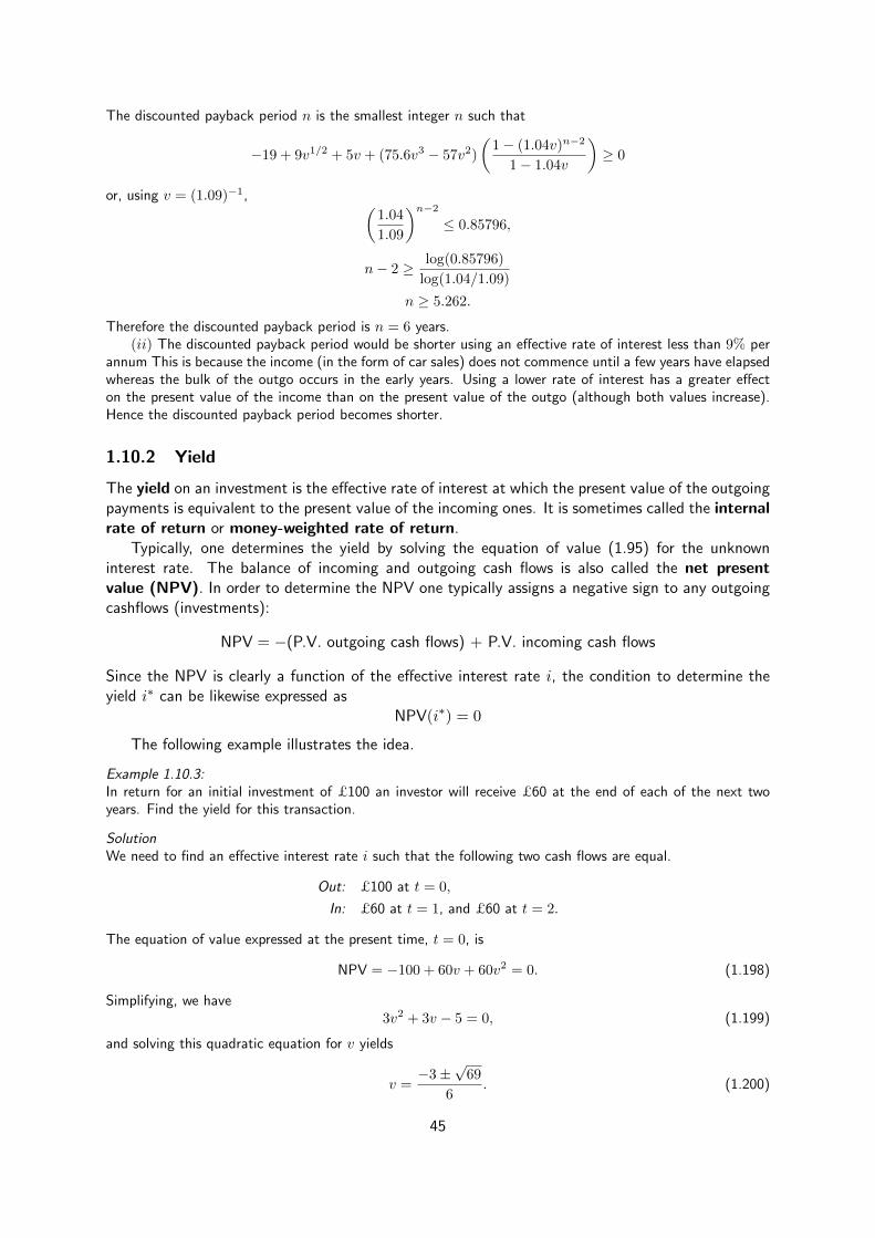
The discounted payback period n is the smallest integer n such that
−19 + 9v1/2 + 5v + (75.6v3 − 57v2)
(1− (1.04v)n−2
1− 1.04v
)≥ 0
or, using v = (1.09)−1, (1.04
1.09
)n−2≤ 0.85796,
n− 2 ≥ log(0.85796)
log(1.04/1.09)
n ≥ 5.262.
Therefore the discounted payback period is n = 6 years.(ii) The discounted payback period would be shorter using an effective rate of interest less than 9% per
annum This is because the income (in the form of car sales) does not commence until a few years have elapsedwhereas the bulk of the outgo occurs in the early years. Using a lower rate of interest has a greater effecton the present value of the income than on the present value of the outgo (although both values increase).Hence the discounted payback period becomes shorter.
1.10.2 Yield
The yield on an investment is the effective rate of interest at which the present value of the outgoingpayments is equivalent to the present value of the incoming ones. It is sometimes called the internalrate of return or money-weighted rate of return.
Typically, one determines the yield by solving the equation of value (1.95) for the unknowninterest rate. The balance of incoming and outgoing cash flows is also called the net presentvalue (NPV). In order to determine the NPV one typically assigns a negative sign to any outgoingcashflows (investments):
NPV = −(P.V. outgoing cash flows) + P.V. incoming cash flows
Since the NPV is clearly a function of the effective interest rate i, the condition to determine theyield i∗ can be likewise expressed as
NPV(i∗) = 0
The following example illustrates the idea.
Example 1.10.3:In return for an initial investment of £100 an investor will receive £60 at the end of each of the next twoyears. Find the yield for this transaction.
SolutionWe need to find an effective interest rate i such that the following two cash flows are equal.
Out: £100 at t = 0,
In: £60 at t = 1, and £60 at t = 2.
The equation of value expressed at the present time, t = 0, is
NPV = −100 + 60v + 60v2 = 0. (1.198)
Simplifying, we have3v2 + 3v − 5 = 0, (1.199)
and solving this quadratic equation for v yields
v =−3±
√69
6. (1.200)
45

Since i > −1, then v must be positive. Hence we take the positive root of (1.200) and finally obtain
i =1
v− 1 = 0.1306623 (to 7 d.p.) (1.201)
So the yield on the transaction is 13.07% p.a. (to 2 d.p.).
Linear Interpolation for the yield
When the yield cannot be solved for explicitly, numerical techniques such as linear interpolationcan be useful. If we know that the NPV is positive for i = i1 and that the NPV is negative for i = i2,where i1 < i2, then the yield i∗ must lie between i1 and i2. If the function NPV(i) is approximatelylinear in i, then
NPV(i∗)−NPV(i1)
NPV(i2)−NPV(i1)≈ i∗ − i1i2 − i1
Since NPV(i∗) = 0, we have
i∗ ≈ i1 + (i2 − i1)×NPV(i1)
NPV(i1)−NPV(i2)(1.202)
Example 1.10.4:Based on a question from the CT1 Exam for April 2013.For an investment of £97, an investor will receive £6 at the ends of the first two years and £109 at the endof the third year. What is the yield?
SolutionThe net present value of the cash flow stream is
NPV(i) = −97 + 6(1 + i)−1 + 6(1 + i)−2 + 109(1 + i)−3. (1.203)
We note that for i1 = 8%, NPV(i1) = 0.227 and that for i2 = 9%, NPV(i2) = −2.277. Plugging into (1.202)shows that the yield is approximately
0.08 + 0.01× 0.227
0.227 + 2.277= 0.08091 (1.204)
or 8.09% p.a. (The exact answer is 8.089% p.a.)
Existence of yield
In some cases the equation of value, with v as the unknown, may have no roots or more than onepositive root and then the yield does not exist. However, the following statements can be made:
• If all negative cash flows precede all positive cash flows (or vice versa) the yield is always welldefined, i.e., there is a unique positive root for v (corresponding to a unique solution withi > −1).
• For a cash flow consisting of amounts ct0 , ct1 , ct2 , . . . , ctn at times t0, t1, t2, . . . , tn thenlet us define the cumulative total amount Ai =
∑ir=0 ctr . If A0 and An are both non-zero
and, excluding zero values, the sequence {A0, A1, . . . , An} contains precisely one change ofsign, then the equation of value has a unique positive solution for i (but there may be otherpositive roots for v corresponding to −1 < i ≤ 0).
See pages 38–40 of [MS86] for further discussion of these important classes of transaction.
46

1.11 Immunisation of cash flows
Suppose an institution receives assets of present value BA to meet liabilities of present value BL.Since both BA and BL represent future cash flows, they are sensitive to changes in the interestrates. If interest rates fall, both BA and BL increase. If interest rates increase, both BA and BLfall. How can you ensure that the value of assets is able to cover the value of liabilities if interestrates fall or increase? This is referred to as immunisation in the context of actuarial mathematics.
Consider a cash flow {b1, ..., bn} of payments made at the end of each year over n years. LetB(i) denote the present value of the cash flow as a function of the effective interest rate i:
B(i) =n∑j=1
bjv(i)j , v(i) =1
1 + i. (1.205)
We want to calculate the change in B(i) following a small change ε in the interest rate i. Therelative change of B(i) is
∆B =B(i+ ε)−B(i)
B(i).
Consider Taylor’s theorem to approximate a general function f(x) around a point x0:
f(x) = f(x0) + f ′(x0)(x− x0) +1
2f ′′(x0)(x− x0)2 + ...
for small deviations x − x0. Setting x = i + ε and x0 = i = const, we obtain for the functionB(i+ ε) the expansion
B(i+ ε) = B(i) +B′(i)ε+1
2B′′(i)ε2 + ...
and the relative change is
∆B =1
B(i)
(B′(i)ε+
1
2B′′(i)ε2
)= −ν(i)ε+
1
2c(i)ε2.
Here, we introduce two quantities
1. The effective duration ν(i) is defined as
ν(i) = − 1
B(i)B′(i)
With Eq. (1.205) the effective duration can be calculated explicitly as
ν(i) = − 1
B(i)B′(i) = − 1
B(i)
d
di
n∑j=1
bjv(i)j
= − 1
B(i)
n∑j=1
bjjv(i)j−1v′(i)
=1
B(i)
n∑j=1
bjjv(i)j+1,
since v′(i) = − 1(1+i)2
= −v(i)2.
47

2. The convexity c(i) is defined as:
c(i) =1
B(i)B′′(i)
Using the expression for B(i), it can be calculated as
c(i) =1
B(i)B′′(i) =
1
B(i)
d
di
− n∑j=1
bjjv(i)j+1
=
1
B(i)
n∑j=1
bjj(j + 1)v(i)j+2
The institution is immunised against small changes in the interest rate, i.e., it can still cover theliabilities, if
1. BA(i) = BL(i), that is, the assets meet the liabilities in the present. The company can ensurethis from the onset, since i is known.
2. BA(i+ ε) ≥ BL(i+ ε), that is, upon a change in the interest rate by ε (positive or negative)the value of the assets is greater or equal that the values of the liabilities.
The conditions such that 2. holds can be formulated more precisely. Consider the surplus S(i) =BA(i)−BL(i). Taylor’s theorem yields for small ε up to quadratic order
S(i+ ε) ≈ S(i) + S′(i)ε+1
2S′′(i)ε2.
We want S(i+ ε) ≥ 0 for immunisation. Consider each term in the Taylor expansion separately.
• 1st term: we have S(i) = 0 since BA(i) = BL(i) for unchanged interest rate.
• 2nd term: both S′(i) and ε can be positive or negative. Impose S′(i) = 0. This term is zeroif
B′A(i) = B′L(i)
⇔ − 1
BA(i)B′A(i) = − 1
BL(i)B′L(i)
⇔ νA(i) = νL(i),
since BA(i) = BL(i). We require the effective durations to be equal.
• 3rd term: the term ε2 is always positive. Thus S′′(i)ε2 is guaranteed positive, if we imposeS′′(i) ≥ 0. This yields
B′′A(i) ≥ B′′L(i)
⇔ 1
BA(i)B′′A(i) ≥ 1
BL(i)B′′L(i)
⇔ cA(i) ≥ cL(i).
We require the convexity of BA to be greater or equal than the convexity of BL.
Overall, we obtain the three conditions for Redington’s immunisation, named after theBritish actuary Frank M. Redington (1906 - 1984):
48
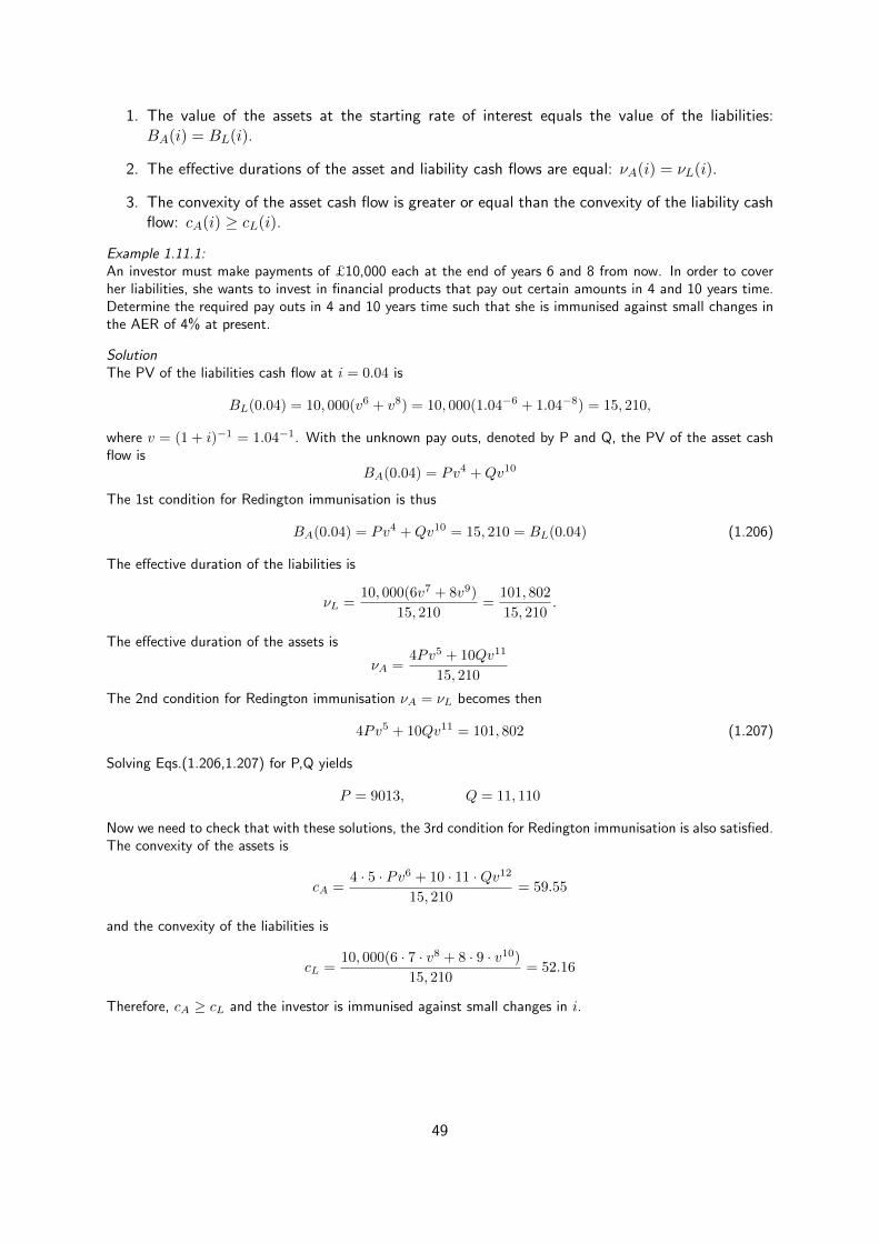
1. The value of the assets at the starting rate of interest equals the value of the liabilities:BA(i) = BL(i).
2. The effective durations of the asset and liability cash flows are equal: νA(i) = νL(i).
3. The convexity of the asset cash flow is greater or equal than the convexity of the liability cashflow: cA(i) ≥ cL(i).
Example 1.11.1:An investor must make payments of £10,000 each at the end of years 6 and 8 from now. In order to coverher liabilities, she wants to invest in financial products that pay out certain amounts in 4 and 10 years time.Determine the required pay outs in 4 and 10 years time such that she is immunised against small changes inthe AER of 4% at present.
SolutionThe PV of the liabilities cash flow at i = 0.04 is
BL(0.04) = 10, 000(v6 + v8) = 10, 000(1.04−6 + 1.04−8) = 15, 210,
where v = (1 + i)−1 = 1.04−1. With the unknown pay outs, denoted by P and Q, the PV of the asset cashflow is
BA(0.04) = Pv4 +Qv10
The 1st condition for Redington immunisation is thus
BA(0.04) = Pv4 +Qv10 = 15, 210 = BL(0.04) (1.206)
The effective duration of the liabilities is
νL =10, 000(6v7 + 8v9)
15, 210=
101, 802
15, 210.
The effective duration of the assets is
νA =4Pv5 + 10Qv11
15, 210
The 2nd condition for Redington immunisation νA = νL becomes then
4Pv5 + 10Qv11 = 101, 802 (1.207)
Solving Eqs.(1.206,1.207) for P,Q yields
P = 9013, Q = 11, 110
Now we need to check that with these solutions, the 3rd condition for Redington immunisation is also satisfied.The convexity of the assets is
cA =4 · 5 · Pv6 + 10 · 11 ·Qv12
15, 210= 59.55
and the convexity of the liabilities is
cL =10, 000(6 · 7 · v8 + 8 · 9 · v10)
15, 210= 52.16
Therefore, cA ≥ cL and the investor is immunised against small changes in i.
49

50

Chapter 2
Fixed Interest Securities and OtherInvestments
We now turn to the different classes of assets that insurance companies, pension funds and individualsinvest in. For the purposes of this module, the classes considered are cash, fixed interest securities,index-linked securities, equities and property. Individual investors may invest directly or through acollective investment product offered by an investment management firm; examples of collectiveinvestment products include ISAs (UK only), unit trusts, investment trusts and exchange tradedinstruments. Large corporate investors are likely to hold most investments directly, using collectiveinvestment vehicles only for more specialised investment holdings.
2.1 Fixed Interest Securities
Governments, local authorities and companies borrow longer term funds by selling bonds (or fixedinterest securities) carrying defined levels of interest payments and defined repayment dates. Thebuyer of a bond is entitled to a fixed series of interest and capital repayments, but assumes the riskthat the borrower (sometimes termed the issuer) will be unable to make the contractual repayments(eg perhaps because of the bankruptcy of a corporate issuer or due to the financial problems of asovereign borrower such as Greece in recent years). Government bonds sometimes have commoninformal trading names such as gilts (UK), Treasuries (USA), Bunds (Germany) and JGBs (Japan).Bonds issued by companies are known as corporate bonds.
Bonds issued by government and large companies are usually listed on a recognised stock ex-change and may be freely traded between investors, meaning that prices of bonds fluctuate fromday to day according to fluctuations in market interest rates and changes in the perceived level ofrisk attached to the repayment of interest and principle by the issuer of the bond. For example, atthe time of writing, many bonds issued by the Greek government trade at much lower prices thanequivalent Bunds reflecting continuing concerns over the ability of the Greek government to repaydebt.
It should be noted that many bonds are bought by investors such as insurance companies andpension funds to match the liabilities of their business; these businesses often follow ”buy and hold”strategies with the result that trading levels can be low for many bonds. This means that marketliquidity (the ease with which significant quantities of the investment can be bought or sold withoutmaterially changing the price) can be limited for many bonds apart from those issued by majorgovernments and the largest companies.
51
2.1.1 Bond Terminology
It is important to understand the terminology used to describe fixed interest securities:
• The nominal amount of a holding is used to define the maturity and interest payments. Theprice of UK gilts is usually quoted per £100 nominal. Bonds are usually traded in integermultiples of the nominal amount.
• The coupon rate defines the interest payable on the bond. The annual interest paid to aninvestor is found by multiplying the coupon rate by the nominal amount of the bond holding.Interest payments are called coupons and typically take place twice per year.
• The redemption price is the amount repaid at maturity (or redemption date) per unitnominal. If the redemption price is 1.00 then the bond is said to be redeemed at par.
• The running yield is the annual interest paid per £100 nominal divided by the market valueof the bond per £100 nominal; this is a measure of the immediate cash return to the investor.
• The gross redemption yield (or GRY) on a bond is the average annual pre-tax return to aninvestor who buys a bond at the current market price and holds the bond to maturity. Anexample of the calculation of GRY is given below.
• A zero coupon bond is a bond that consists only of a redemption payment; there are nointerest payments. A Treasury Bill (see section 2.2) is a simple example of a zero couponbond.
• An undated bond or perpetuity has no redemption date.
2.1.2 Example of a Government Security
The 2.75% Treasury Gilt 2024 is a typical conventional UK government security; note that therepayment year and the annual coupon rate are referenced in the name of the the security. Keyfeatures include:
• The gilt is bought or sold in units of £100 nominal, in common with most gilts.
• The gilt is repayable at par (ie £100 per £100 nominal) on 7 September 2024.
• The gilt was first sold by the Debt Management Office on behalf of the UK Treasury on 12March 2014, so the initial term was around 10.5 years. The initial price was £98.40 per £100nominal; ie a little below par.
• The gilt was issued on a number of other occasions up to January 2015; the total nominalamount issued to date is £27 billion.
• In common with most gilts, interest payments are made twice yearly in arrears; in this case on7 March and 7 September. The last coupon is paid on the date of repayment of the bond.The coupon is £2.75 per £100 nominal meaning that the six monthly interest payment is£1.375 per £100 nominal.
52
2.1.3 Types of Corporate Bonds
There are many different types of corporate bonds available; investors need to pay attention to theprecise features of each bond as these will influence the bond’s risk characteristics and its value toan investor. Particular types to be aware of include:
• Debenture A debenture is a corporate bond offering some additional security to the investorover and above the ability of the company to continue to trade profitably.
• Unsecured loan stock Unsecured loan stock offers no additional security to investors andrepayments of interest and capital depend on the ability of the issuing company to generateprofits to make repayments. In the event that the issuer becomes insolvent, investors wouldrank alongside other unsecured creditors such as suppliers.
• Convertible bonds A convertible bond is a bond that is convertible into a different form ofsecurity in certain circumstances. For example, since the 2007/2008 financial crisis, banks andinsurance companies have been encouraged to issue bonds which convert into equity shares ifthe bank or insurance company is unable to meet certain solvency thresholds.
• Asset backed securities There are a wide range of bonds backed by underlying cashflowsdue to a bank or other financial institution; for example the repayments due under mortgageloans, credit card loans or student loans. Non financial cashflows can also be used to backbond investments; examples range from usage charges on infrastructure projects, the emergingprofits of a book of life insurance policies to the royalties arising from David Bowie’s music.The process of taking an illiquid or non-financial asset and structuring it into one or moresecurities is often termed securitisation.
2.1.4 Valuation of a Bond
In relation to a corporate bond let us define:N =the notional amount of bond that is used to define interest and repayment amounts (e.g. £100);D = the annual coupon rate on the bond, payable twice yearly in arrears (e.g. 4%);p = the coupon payment frequency per year (usually p = 2);n = the term to maturity of the bond; andR = the repayment amount as a percentage of the notional amount of the bond (e.g. 110%)
The price of the bond per N nominal at a gross redemption yield (or interest rate) of i p.a.is given by the equation of value:
Price = Present value of future coupon payments + Present value of future capital repayments
(2.1)
= DNa(p)n +RNvn, where v =
1
1 + i(2.2)
Example 2.1.1: Valuation of a BondOn 5th April 2017, the 3.75% UK Corporate Bond 2024 is trading at a gross redemption yield of 1.4% p.a.The repayment date is 5th September 2024 and repayment is at 110% of nominal. The coupon is paidsemi-annually on the anniversary of the repayment date. Calculate the price of the bond per £100 nominal.
SolutionNote that at the valuation date, the bond has 7 years and 5 months (or 153 days) to run until maturity, andthat the next coupon will be paid in 5 months time.
53

Then, by substituting in (2.2), and adjusting for the fact that coupon payments will be received in respectof 7.5 years, the price per £100 nominal is:
Price per £100 nominal = 100(.0375)(1 + i)112 a
(2)
7.5+ 100(1.10)v7+5/12 at i = 1.40% pa
= 3.75(1.014)112
1− (1.014)−7.5
2(1− (1.014)−0.5)+ 110(1.014)−7.41667
= 26.647 + 99.223
= £125.87 to the nearest penny.
Example 2.1.2: Calculating the Gross Redemption YieldOn 5th January 2017, the UK Treasury 8.75% 2017 gilt is trading at £108.50. The repayment date is 25thAugust 2017 and the coupon is paid semi-annually. Calculate the gross redemption yield available to aninvestor, assuming that repayment will be at par (ie at £100 per £100 nominal).
SolutionThe price quoted is per £100 nominal. Note that the gilt is trading above par and the the investor will facea capital loss at maturity. This reflects how interest rates have fallen since the gilt was issued at a price of£97.38 on 30th April 1992.
The six monthly interest payment per £100 nominal is £4.375 (= 0.0875 × 100/2). Interest paymentswill be on February 24th (50 days) and August 25th (232 days).
The gross redemption yield(GRY) to the investor is then i where i is the solution to the equation of valuedeveloped from (2.2):
F (i) = 108.50 = 4.375(1 + i)−50/365 + (100 + 4.375)(1 + i)−232/365
The GRY i will be found by iteration. By inspection, you can see that the GRY is close to zero sinceF (0) = 108.75. So, we will take i1 = 0.00 as our first estimate of i. We aim to find a second estimate ofthe GRY, i2, such that F (i2) < 108.50. For our next estimate we take i2 = 0.005, as using an estimate of1.0 for i is likely to reduce the calculated price by almost £1 which would be too much.
F (0.005) = 108.42 which is less than 108.50 as desired.The next iteration i3 is therefore estimated by interpolation as:
i3 = i1 + (i2 − i1)
[108.50− F (i1)
F (i2)− F (i1)
[= 0.00 + .005
[108.50− 108.75
108.42− 108.75
[= 0.0038 to 2 significant figures
Testing this new trial value, we find F (0.0038) = 108.50 to 2 decimal places. Therefore the GRY is0.38% to 2 significant figures.
Summary of 2.1
Value of Bond per N nominal = N[Da
(p)n +Rvn
]D is the annual coupon rate paid twice yearly in arrears;p is the coupon payment frequency per year;R is the repayment amount as a multiple of the nominal amount (frequently R will be 1.00);n is the term to maturity of the bond in years; andi is the gross redemption yield (or pre tax return) on the bond.
2.2 Cash including Treasury Bills
As an investment class, cash includes not only money held in current accounts with banks butalso a wider class of investments known as money market instruments. These are short terminvestments (typically less than 1 year and usually much shorter) with low risk and high liquidity (iereadily traded). The most common types of instrument are:
54

• Certificates of Deposit issued by banks and building societies for terms usually ranging from28 days to 6 months. Interest is paid on the maturity of the contract.
• Commercial Paper issued by major companies to finance their short term borrowing needs. Inthe UK, the term of commercial paper is limited to one year; while in the USA the limit is 270days.
• Treasury Bills issued by governments. These bills do not pay interest, but are usually sold bygovernments for less than the nominal (or ”face”) value. The investor earns a positive returnby purchasing a bill for less than its nominal value or ”less than par” and receiving the fullpar value at redemption. At times of very low interest rates, Treasury Bills sometimes tradeat ”over par” meaning that the investor earns a negative return for holding this low risk cashinvestment.
In the UK, the Government’s Debt Management Office (DMO) sells Treasury Bills on at least aweekly basis through an auction process. UK Treasury Bills are usually issued for terms of 1, 3 or 6months.
Example 2.2.1: Returns on Treasury BillsA investor buys a 6 month (182 day) Treasury Bill for £98.75 per £100 nominal. Find the annual effectiverate of return that the investor realizes if the bill is held to maturity.
SolutionReturn earned over 182 days per £100 nominal = £1.25 (= 100.00 − 98.75) or 1.2658% (= 1.25/98.75 ×100%).Annual compound return = (1 + 1.25/98.75)365/182 - 1 = 2.5548%
2.3 Inflation Linked Bonds and Real Returns
Inflation linked bonds or index-linked bonds are a type of bond for which interest and capitalrepayments are fixed not in currency terms but relative to an index of inflation. If inflation is positive,the bond holder receives an increasing stream of coupon payments and a repayment amount thatwill be greater than the nominal value of the bond. The attraction to issuers is that the initial costsof servicing (paying the coupons) an index-linked bond will usually be lower than for a fixed interestbond; while for an investor an index-linked bond is a hedge against inflation risk and perhaps anatural match to some types of liabilities. In the UK, most UK Index-Linked gilts are held bypension funds and insurance companies to help match the inflation linked payments made by manypension schemes.
Financial Calculations in Real Terms
To date, all calculations in this document have been defined in terms of known monetary amounts.However, with inflation, the amount of goods and services purchased by a fixed amount of moneypayable at some future date is unknown. In general, prices tend to rise as a result of inflation in theeconomy; in recent years, central bankers have typically tried to target inflation rates in the rangeof 2% to 3% per annum. This means that the ”purchasing power” of a fixed sum of money declinesover time.
Sometimes, financial calculations are made in ”real terms” rather than monetary terms; some-times this is referred to as assuming constant prices.
The first step is to adjust monetary calculations to a common price point, using an inflationindex Q(t). For example, if Ct2 is a monetary cashflow payable at time t2, then the ”real value” of
55

the cashflow in terms of prices at time t1 is given by:
Real value of cashflow in terms of t1 prices = Ct2Q(t1)
Q(t2)(2.3)
This is often termed the cashflow in terms of ”t1 money”.If Ct2 is a future cashflow, and the inflation index after t1 is not yet determined, then we assume
a future rate of inflation of j% p.a. and write:
Q(t2) = Q(t1)(1 + j)t2−t1 for t2 > t1. (2.4)
Sometimes, we will use a combination of known values and assumed future inflation to determinethe inflation index. For example, if ta is the last date for which the inflation index is known, then:
Q(t2) = Q(ta)(1 + j)t2−ta where t1 < ta < t2 and (2.5)
Real value of cashflow in terms of t1 prices = Ct2Q(t1)
Q(ta)(1 + j)t2−tafrom 2.4 (2.6)
2.3.1 Calculating the Real Rate of Return
The internal rate of return (IRR) is the rate of interest at which the present value of all (positive andnegative) cashflows is zero. Similarly, the real rate of return is the rate of interest at which thepresent value of all real cashflows (or ”constant price” cashflows) is zero. Given a series of monetarycashflows Ct for t = t0 to tn and an inflation index Q(t), the real rate of return is i′ where:
tn∑t=t0
Ct
[Q(t0)
Q(t)
](1 + i′)−(t−t0) = 0 (2.7)
If all future values of the inflation index are based on an assumed rate of future price inflationj, then 2.7 becomes:
tn∑t=t0
Ct
[Q(t0)
Q(t0)(1 + j)t−t0
](1 + i′)−(t−t0) = 0 from 2.4
⇒tn∑t=t0
Ct1
[(1 + j)(1 + i′)]t−t0= 0
⇒tn∑t=t0
Ct1
(1 + i)t−t0= 0 where i = (1 + j)(1 + i′)− 1.
This equation is the usual equation for the present value of a series of cashflows, and from thiswe can derive the relationship between:
• j, the assumed rate of future inflation;
• i′, the real rate of return; and
• i, the monetary rate of return (usually just termed the interest rate or yield on an investment)
1 + i = (1 + i′)(1 + j); or (2.8)
i = i′ + j(1 + i′); or (2.9)
Real rate of return, i′ =i− j1 + j
(2.10)
56

Example 2.3.1: Real rate of ReturnAn investor buys a bond with a gross redemption yield of 4.5% p.a. If future price inflation is expected to be0.5% p.a. above the central bank target rate of 2.5%, calculate the expected real return on the bond.
Solution
Expected future inflation,j = .025 + 0.005 = 0.030
Expected real return,i′ =i− j1 + j
from 2.10
=.045− 0.030
1.03= 0.0146 to 3 significant figures.
The expected real return from the investment is therefore 1.46% p.a. Note that if expected future inflationis low then i′ ≈ i− j.
2.3.2 Valuation of Index-Linked Bonds
The biggest issuer of index-linked bonds in the UK is the government; these are termed ”index-linkedgilts”. For example, the UK Government first issued the 1.25% Index-Linked Treasury Gilt 2017 on8th February 2006. The gilt is repayable on 22 November 2017 and coupon payments are made halfyearly on 22nd May and 22nd November. Redemption payments per £100 nominal are given by theformula:
RedemptionPayment = 100× Index(22.11.2017)
Index(8.2.2006)(2.11)
Similarly, each coupon payment is indexed using the formula:
CouponPayment(coupondate) = 100× 0.0125/2× Index(coupondate)
Index(8.2.2006)(2.12)
where Index(date) is the value of the Retail Prices Index 3 months before date. This reflects thatRPI is determined in arrears and that for practical reasons all bond payments must be determinedfrom a known index that will be (at least fractionally) out of date. This is referred to a 3 monthdeferment or time-lag (or just lag).
The RPI Index for November 2005 was 193.6 and the index had increased to 259.8 by August2015 (3 months prior to the November 2015 payment date). The coupon paid in November 2015per £100 nominal was £0.8387 (= 0.0125/2× 100× 259.8
193.6).To calculate the real return on an index-linked bond it is necessary to make assumptions about
the rate of future inflation. The Financial Times publishes real yields for UK index-linked benchmarkgilts assuming future inflation of 0% per year and 5% per year.
Assuming no time-lag (or deferment) in the calculation of indexation, the price of £N nominalof an index-linked bond at time zero at an effective monetary yield of i can be found by discountingthe expected monetary payments at the assumed monetary yield:
Price at time 0 =2n∑k=0
D
2NQ(k/2)
Q(0)vk/2i +RN
Q(n)
Q(0)vni (2.13)
where
• D is the nominal annual coupon rate paid twice per year in arrears;
• R in the nominal repayment amount per N nominal;
57

• n is the term to run in years; and
• Q(t) is the value of the price index at time t.
On the assumption, that there is no lag in indexation, then the price of an index-linked bond at areal return of i′ is simply
Price at time 0 =
2n∑k=0
ND
2vk/2i′ +NRvni′ (2.14)
= DNa(2)n
∣∣∣@i=i′
+NRvni′ (2.15)
where vi′ = 1/(1 + i′).
At some time t1 after issue, t1 > 0 the nominal amount has to be converted to the real amountat t1:
Price at time t1 =2n∑k=t1
D
2NQ(k/2)
Q(t0)vk/2i +RN
Q(k/2)
Q(t0)vni (2.16)
=
2n∑k=t1
D
2NQ(t1)
Q(t0)
Q(k/2)
Q(t1)vk/2i +RN
Q(t1)
Q(t0)
Q(k/2)
Q(t1)vni (2.17)
=Q(t1)
Q(t0)
[DNa
(2)
n−t1
∣∣∣@i=i′
+NRvni′]
(2.18)
The valuation of the bond is thus based on nominal real amounts at the real rate of return.
Example 2.3.2: Valuation of an Index-Linked BondOn 1 January 2013, a government issued a 5 year index-linked bond with a nominal coupon of 3% per annumpayable half yearly in arrears. The nominal redemption price is 100%. A non-tax paying investor buys £1000nominal on 20 January 2017 and holds to maturity. Bond payments are indexed with a 3 month time lag.Relevant values of the Retail Prices Index are given in the table below:
RPI 2012 2013 2016 2017 2018Jan 144.1 150.90 170.0 175.6
April 145.0 151.40 171.4July 147.4 167.6 172.7Oct 149.2 169.4 173.8
1. Calculate the coupons and the redemption payment that the investor receives.
2. Calculate the price that the investor pays for the bond if the real return to the investor is 3.5% pa.
Solution 1. The investor receives the coupons paid on July 1 2017 and the final coupon and redemptionpayment on January 1 2018. Due to the 3 month indexation lag, the relevant values of the Index arethe values for October 2012 (for indexation of the nominal values at issue) and the values in April andOctober 2017.
Coupon received July 2017 = 1000×[.03
2
] [Index(Apr17)
Index(Oct12)
](2.19)
= 15
[171.4
149.2
](2.20)
= £17.42 to the nearer penny. (2.21)
58

and similarly, the final coupon and redemption payment are found from:
Final Coupon and Redemption Payment = (1000 + 15)
[Index(Oct17)
Index(Oct12)
](2.22)
= 1015
[173.8
149.2
](2.23)
= £1182.35 to the nearer penny. (2.24)
2. To determine the price the investor paid for the bond, we:
• convert the monetary cashflows into constant (or real) price terms, using the January 2017 RPIvalue ; and
• discount the real cashflows using the investor’s real investment return of 3.5% and the usual bondpricing formula (2.14).
Cashflows are converted to ”January 17” prices in the table below:
Date Monetary Amount in RealAmount ”Jan 17” Money Cashflow
July17 17.42 = 17.42× Index(Jan17)Index(July17)
17.42 × 170.0172.5 = 17.16
Jan18 1182.35 =1182.35× Index(Jan17)Index(Jan18)
1182.35 × 170.0175.6 =1144.64
The first cashflow is paid after 162 days, while the redemption proceeds and final coupon are receivedafter 346 days. Therefore, the price of bond to give a real return of 3.5% pa is given, using (2.14), by:
Price = 17.16(1.035)−162365 + 1144.64(1.035)−
346365
= 1124.81 to the nearer penny.
Summary of 2.3
Real rate of return, i′ = i−j1+j
where i is the monetary rate of return and j is the expected rate of future inflation.
To determine, the real rate of return from a series of monetary cashflows, Ct, firstconvert monetary cashflows to real (or constant price) cashflows, using theappropriate Index values, allowing for any specified time-lag in indexation, andthen determine the real rate of return following usual iterative approaches.
2.4 Equities
Equities represent the shares of companies. These may be large household names such as BP,Barclays Bank or Tesco plc whose shares are traded on the London Stock Exchange(LSE) and areconstituent companies in the FTSE100 index, which is the most widely quoted UK stock marketindex. Smaller, lesser known companies are also traded on the LSE and on its sister market AIM(formerly known as the Alternative Investment Market).
Shares listed on markets can be readily bought and sold, but there are also thousands of smallprivate companies that are not listed. Institutions will also invest in private unlisted companieswith the intention of being a shareholder for several years before the company is sold or listed on arecognised stock exchange; this form of investment is usually termed venture capital.
59

Characteristics of Ordinary Shares
When we talk of shareholders, we are usually referring to the holders of the ordinary shares in thecompany. The key characteristics of ordinary shares include:
• The holders of the ordinary shares are the owners of the company; they have the responsibilityfor appointing the directors; approving the accounts; and agreeing all major decisions (suchas a decision to sell the company).
• The shareholders benefit from the residual profits of the company, after bond holders and anypreference shareholders have been paid, and have to decide on the level of profit to be heldback by the company to fund future growth (”retained earnings”) and the amount of profitto be distributed to shareholders as dividends.
• Ordinary shareholders receive a return on their investment in the ordinary shares of a companythrough dividend payments and through increases (or falls) in the value of the shares.
• Ordinary shares are usually considered to be the class of investment providing the highest riskand, potentially, the highest return to an investor.
• In the event of the insolvency of the company, ordinary shareholders will only receive moneyafter all other creditors including bond holders, have been paid. In this situation, shareholdersfrequently receive nothing.
• Shares in large quoted companies are highly marketable with low transaction costs.
2.4.1 Valuation of Shares by Discounting Future Dividends
Valuing ordinary shares is a matter of art as well as science and a full treatment of the many differentapproaches is beyond the scope of this module. We will however, apply our knowledge of compoundinterest to look at the discounted dividend model of share valuation.
In the simplest form, we assume that dividends are payable annually in perpetuity. If Dt is thedividend payable at time t, and the next dividend is payable in 1 year’s time, then the value of oneshare at an interest rate of i is found by by discounting future cashflows:
Value of share =∞∑t=1
Ctvt (2.25)
It is common to assume that dividends grow at a constant rate of g pa. Then if D is the lastdividend paid, we can write Dt = D(1 + g)t. Discounting future cashflows we get:
Value of share =
∞∑t=1
Ctvt (2.26)
=
∞∑t=1
D(1 + g)t(1 + i)−t (2.27)
= Dai′∞ where (1 + i′) =
1 + i
1 + g(2.28)
= D1
i′using formula for value of a perpetuity (2.29)
Value of share = D(1 + g)
(i− g)(2.30)
60

This is sometimes termed the dividend growth model. In practice, the valuation of future dividendswill depend on the precise timing on cashflows. Shares can be sold ”cum div” meaning with thenext dividend payment or ”ex div” meaning without the next payment. For practical reasons, sharesoften trade ”ex div” several weeks before the dividend payment is actually paid.
Sometimes, investors will make more complex assumptions about the rate of future dividendgrowth as in example below.
Example 2.4.1: Share ValuationA pension fund, not subject to tax, is considering buying a share whose last annual dividend was 15p pershare. The fund expects dividends to grow by 10% pa for the next 10 years and to be able to sell the sharesafter 10 years at a price that will give the purchaser a yield of 5% on the purchase price ( a ”dividend yield”).The next dividend is due in one year’s time. What price should the fund pay to achieve a return of 8% pa ontheir investment if the assumptions are achieved in practice?
SolutionThe value of the share to the investor is the sum of the present value of the expected dividend payments over10 years plus the present value of the share price after 10 years (since the plan is to sell the shares then).
PV(Dividends for 10 years) =
10∑t=1
D(1 + g)tvt
=
10∑t=1
0.15(1.10)t(1.08)−t
= 0.15(1.10)(1.08)−1[
1− (1.10)10(1.08)−10
1− 1.10(1.08)−1
]= 1.66 to 2 decimal places
Share Price after 10 Years =Dividend in 10 Year’s Time
Yield at Sale Price
=0.15(1.10)10
.05= 7.78
Value of Share = 1.66 + 7.78v10
= 1.66 + 7.78(1.08)−10
= 5.26 to 2 decimal place
The value of the share is £5.26 on the assumptions given.
2.4.2 Characteristics of Preference Shares
A lesser known class of shares is preference shares. For any given company, preference shares willbe considered as a higher risk investment than a corporate bond, but a lower risk investment thanordinary shares. The key characteristics of preference shares include:
• Preference shares carry a fixed rate of dividend, meaning that shareholders do not usuallybenefit from the profitable growth of the business.
• Dividends can only be paid from profits after all interest costs have been met. Preferenceshareholders must be paid before any dividends can be distributed to the ordinary shareholdersin a company.
61

• In the event that profits are inadequate to pay dividends on preference shares, it is commonfor any unpaid dividend to be carried forward to future years. This type of share is termed acumulative preference share.
• In the event of the insolvency or winding up of the company, the holders of preference shareswill only receive a return of their capital after the amounts due to all other creditors (otherthan ordinary shareholders) have been paid.
• Taking these factors together, it can be seen that the preference shares of a company arelikely to be lower risk than the ordinary (or equity) shares of a company, but higher risk thancorporate bonds issued by the same company.
This class of share introduces no new mathematical questions about valuation. It is important toremember that in the absence of any further information, dividends on preference shares are nonincreasing and are paid in perpetuity
Tax changes in the UK mean that this class of shares is relatively unattractive at present for theissuing company; it is usually cheaper to raise finance through issuing corporate bonds.
2.5 Property
Institutional investors, such as insurance companies and pension funds, have traditionally invested inUK office blocks, shops and industrial units. In recent years, the range of property investments hasexpanded to include international property assets and residential accommodation that is availablefor rent (including student accommodation). Most assets are held on a freehold basis, althoughsome might be on a long leasehold basis. Freehold is a legal term used in property; a freeholder isthe absolute owner of a property. A freeholder may grant an individual the right to use a propertyfor a period of time through agreeing a lease; this is a contract giving the leaseholder a right tooccupy the property for a period of time. For example, new flats in London are frequently sold onthe basis of 99 or 125 year leases; with the developer retaining the freehold.
Investors in property receive a return through the rental income on the property and from changesin the capital value of the property.
As an asset class, property is usually positioned between corporate bonds and equities in termsof risk and return. However, within the property class, there are great variances between differenttypes of investment holding. For example, a prime London office building would be sold on a lowyield in the expectation of future growth in rent levels. In contrast, properties in less successful areasof the UK might be sold on much higher yields reflecting the poor prospects for rental growth andthe difficulty of re-letting the property should the tenant fail or simply not renew the lease.
Other characteristics of property include:
• A balanced property portfolio is likely to have a higher running yield than an equivalent equityportfolio.
• Some properties may be let on long leases, with rent reviews every 3 or 5 years in accordancewith the terms of the lease.
• Some leases may specify that rent reviews are ”upwards only”. Despite the terms of lease-hold agreements, in areas where the demand for property is weak (eg some shopping areas)leaseholders have sometimes been able to negotiate lower rental levels.
• Property investments are typically large, ”lumpy” (meaning that a portfolio valued at say £100million may consist of only a few properties) and expensive, and sometimes difficult, to buyand sell. This means that property is a relatively illiquid asset class.
62
• The illiquidity and individuality of property investments make this a difficult asset class to value;professional independent valuation on a regular basis is required adding to the managementcosts of this asset class.
• Investors must remember the risk of rent ”voids”, when there is no tenant or income for aproperty.
• Properties may require some repair or improvement in order to re-let the property when atenant vacates.
• All of the factors above mean that property has materially higher management costs thanother asset classes.
• The complexity and ”lumpiness” of property means that only the largest pension funds andinsurance companies will manage their own property portfolios; many will contract this roleout to specialist property investment firms or invest via pooled property funds.
No new mathematical techniques are required to value a property investment, or to determine theIRR from an investment. However, the fact that rents may increase every 3 or 5 years can addcomplexity to calculations as shown in the example below.
Example 2.5.1:An investor is considering buying a property with a 25 year lease. The property is tenanted with a currentrental income of £220,000 per year payable quarterly in advance. Rents are reviewed every 5 years and thenext review is in 5 years time. Expenses of management are £1,000 per month payable monthly in arrears.Determine the maximum price that the investor should offer to achieve a pre-tax return of 6% pa, assumingthat the rate of future rental increase will be 2% pa.
SolutionThe maximum price is determined by discounting future expected cashflows at a rate of 6% per annum:
Maximum price = PV(Rent)− PV(Expenses) at a rate of 6% pa
PV(Rent) = 220, 000[a(4)
5+ v5(1.02)5a
(4)
5+ v10(1.02)10a
(4)
5+ v15(1.02)15a
(4)
5+ v20(1.02)20a
(4)
5
]= 220, 000a
(4)
5
[1 + v5(1.02)5 + v10(1.02)10 + v15(1.02)15 + v20(1.02)20
]= 220, 000
[1− 1.06−5
4(1− 1.06−0.25)
] [1− ( 1.06
1.02 )−25
1− ( 1.061.02 )−5
]= 961218.93(3.530623)
= 3, 393, 702 to the nearest £
PV(expenses) = 12, 000a(12)
25= 157, 574 to the nearest £
The maximum price to be paid to achieve a yield of 6% is therefore £3,236,128.
2.6 Taxation
The rules of taxation are complex and different for individuals, companies, insurance companies andpension funds. Detailed tax rules and tax rates are set by nation states and vary significantly acrossthe globe, and are outside of the scope of this course. This section introduces the concepts of thetaxation of income and the taxation of capital gains and includes an example illustrating how taxcan be included into the evaluation of investments.
In earlier sections, we have discussed the yield obtained from a bond investment. Different termsare used depnding on whether a pre-tax or a post-tax return is being calculated:
63

• The Gross Redemption Yield on a bond is the average return to maturity calculated ona pre-tax or a gross basis. No allowance is made for taxation when calculating the grossredemption yield.
• The Net Redemption Yield on a bond is the average return to maturity calculated on a post-tax or a net(of tax) basis. The net redemption yield is calculated allowing for the paymentof tax on income and, if applicable, any tax paid on capital gains.
It should be noted that pension funds are not usually subject to tax on income or capital gains, sothe pension fund receives the full gross return.
2.6.1 Income Tax
Taxpayers, or a company, will often be subject to tax on regular sources of income, including:
• interest on bank accounts;
• coupons paid on government securities and corporate bonds;
• dividends paid on ordinary or preference shares; and
• rental income from properties after allowing for applicable management expenses. ( Manage-ment expenses will usually be tax deductible.)
Example 2.6.1: Valuation of a Bond allowing for Income TaxIf an investor is subject to income tax at the rate t1 then the formula for valuation of a bond with a couponC payable twice-yearly [see (2.2) above] becomes:
Value of bond = (1− t1)CNa(2)
t+RNvt (2.31)
Example 2.6.2: Calculation of after-tax CouponAn investor pays tax on income at the highest marginal rate of 45%. The investor holds £100,000 nominalof a corporate bond with a coupon rate of 4.5% per annum payable twice yearly. What is the net periodiccoupon received by the investor?
Solution
Periodic (six-monthly) coupon = .045× 100000/2
= £2, 250.
Investor’s tax rate = 45%
Net (after-tax) periodic coupon = (1− 0.45)× 2250
= 1237.50 to the nearer penny.
The net periodic coupon received by the investor is £1,237.50 .
2.6.2 Tax on Capital Gains
Investors who sell an asset for a higher price than they purchased it for make (or realise) a capitalgain. Similarly, investors who sell an asset for a lower price than they purchased it realise a capitalloss. Individual investors are often subject to tax on capital gains.
In the UK, individual investors usually pay no tax on capital gains on gilts and other bondholdings, but gains on equity and property holdings are subject to tax. If an investor makes a capitalloss, then that loss can often be used to reduce the taxable gains generated on other investments.No detailed knowledge of the complex rules regarding taxation of capital gains and losses is requiredfor this module. Students should, however, be able to adjust calculations for tax on capital gains asinstructed.
64
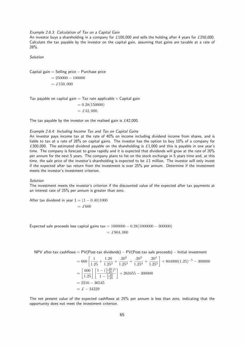
Example 2.6.3: Calculation of Tax on a Capital GainAn investor buys a shareholding in a company for £100,000 and sells the holding after 4 years for £250,000.Calculate the tax payable by the investor on the capital gain, assuming that gains are taxable at a rate of28%.
Solution
Capital gain = Selling price− Purchase price
= 250000− 100000
= £150, 000
Tax payable on capital gain = Tax rate applicable× Capital gain
= 0.28(150000)
= £42, 000.
The tax payable by the investor on the realised gain is £42,000.
Example 2.6.4: Including Income Tax and Tax on Capital GainsAn investor pays income tax at the rate of 40% on income including dividend income from shares, and isliable to tax at a rate of 28% on capital gains. The investor has the option to buy 10% of a company for£300,000. The estimated dividend payable on the shareholding is £1,000 and this is payable in one year’stime. The company is forecast to grow rapidly and it is expected that dividends will grow at the rate of 20%per annum for the next 5 years. The company plans to list on the stock exchange in 5 years time and, at thistime, the sale price of the investor’s shareholding is expected to be £1 million. The investor will only investif the expected after tax return from the investment is over 25% per annum. Determine if the investmentmeets the investor’s investment criterion.
SolutionThe investment meets the investor’s criterion if the discounted value of the expected after tax payments atan interest rate of 25% per annum is greater than zero.
After tax dividend in year 1 = (1− 0.40)1000
= £600
Expected sale proceeds less capital gains tax = 1000000− 0.28(1000000− 300000)
= £804, 000
NPV after-tax cashflows = PV(Post-tax dividends)− PV(Post-tax sale proceeds)− Initial investment
= 600
[1
1.25+
1.20
1.252+
.202
1.253+
.203
1.254+
.204
1.255
]+ 804000(1.25)−5 − 300000
=
[600
1.25
] [1− ( 1.20
1.25 )5
1− 1.201.25
]+ 263455− 300000
= 2216− 36545
= £− 34329
The net present value of the expected cashflows at 25% per annum is less than zero, indicating that theopportunity does not meet the investment criterion.
65

Term Libor (i(p)(t)) p Spot rate sT1 day 0.226 365 0.253
1 month 0.261 12 0.2953 months 0.383 4 0.4426 months 0.548 2 0.623
1 year 0.792 1 0.792
Table 2.1: The £LIBOR rates from Fig. 1.2.2 corresponding to i(p)(t) at t=7.12.2016 and differentterms p. The calculated spot rate for each term is also given.
2.7 The term structure of interest rates
In financial markets, interest rates typically depend on the duration over which money is held. Thisbecomes evident, if we derive interest rates from real financial markets, such as the £LIBOR ratesin Fig. 1.2.2 on 7.12.2016. The rates on this particular day are given in percentages per annum formoney held over different terms such as one day, one month, one quarter, one year. In the contextof the interest rates discussed so far, these correspond to time-dependent nominal interest ratesi(p)(t), where t is the date 7.12.2016 and p = 365, 12, 4, 1, see Table 2.7. If you were to check theLIBOR rates on a different day, these values change, indicating the dependence on t. On the otherhand, the fact that the rates also change with p on any given day highlights the term structure ofinterest rates.
2.7.1 Spot rates
For each of the nominal rates, we can calculate the corresponding annual effective rate withEq. (1.20), which now assumes a different value depending on p. It is customary to set a timeinterval T = 1/p and refer to the annual effective rates over different T as spot rates sT , seeTable 2.7. Thus spot rates and nominal interest rates are related as
1 + s1/p =
(1 +
i(p)
p
)p(2.32)
The function sT is called spot rate curve and characterizes the term structure of interest rates.Spot rates can also be derived from the prices of unit zero coupon bonds with different maturities
T (i.e., bonds without coupon payments and paying 1 unit of money at maturity), see Table 2.7.1.These prices result from trading and thus vary according to supply and demand. If P (T ) is the presentprice of a unit zero coupon bond maturing at time T , the spot rate is given as the correspondingannual effective rate that expresses the discounting of £1 received at time T
P (T ) =1
(1 + sT )T⇒ sT = P (T )−1/T − 1. (2.33)
Typical spot rate curves are increasing with T , but can also assume different shapes dependingon market sentiment. Possible economic explanations for the shape of spot rate curve are:
1. Expectations theory: spot rates are determined by expectations of what interest rates willbe like in the future.
2. Liquidity preference: investors prefer their funds to be liquid (easily accessible). Therefore,bond issuers have to provide incentives for long-term bonds in the form of higher yields.
3. Market segmentation: different investors buy bonds with different maturities. Therefore,the market for the bonds is segmented and prices develop differently.
66
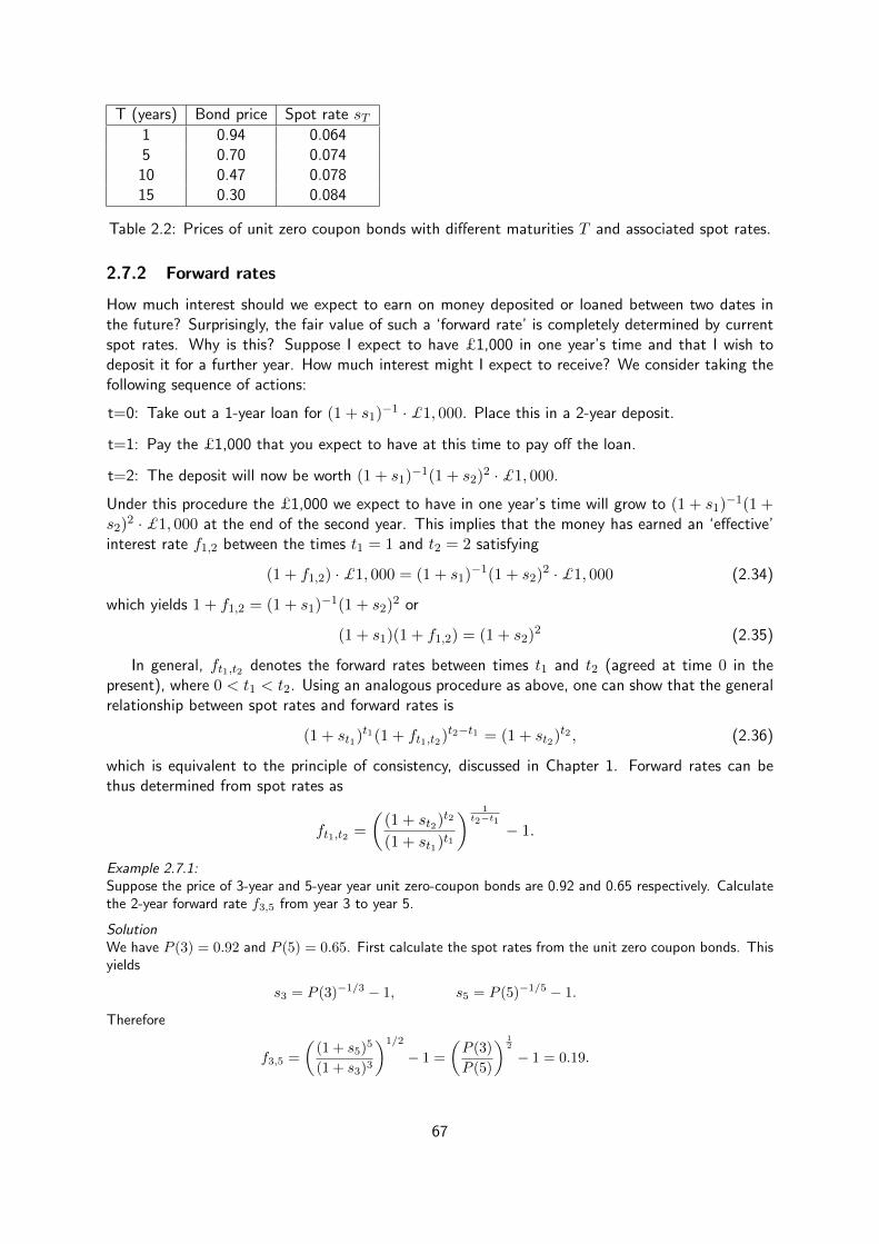
T (years) Bond price Spot rate sT1 0.94 0.0645 0.70 0.074
10 0.47 0.07815 0.30 0.084
Table 2.2: Prices of unit zero coupon bonds with different maturities T and associated spot rates.
2.7.2 Forward rates
How much interest should we expect to earn on money deposited or loaned between two dates inthe future? Surprisingly, the fair value of such a ‘forward rate’ is completely determined by currentspot rates. Why is this? Suppose I expect to have £1,000 in one year’s time and that I wish todeposit it for a further year. How much interest might I expect to receive? We consider taking thefollowing sequence of actions:
t=0: Take out a 1-year loan for (1 + s1)−1 ·£1, 000. Place this in a 2-year deposit.
t=1: Pay the £1,000 that you expect to have at this time to pay off the loan.
t=2: The deposit will now be worth (1 + s1)−1(1 + s2)
2 ·£1, 000.
Under this procedure the £1,000 we expect to have in one year’s time will grow to (1 + s1)−1(1 +
s2)2 ·£1, 000 at the end of the second year. This implies that the money has earned an ‘effective’
interest rate f1,2 between the times t1 = 1 and t2 = 2 satisfying
(1 + f1,2) ·£1, 000 = (1 + s1)−1(1 + s2)
2 ·£1, 000 (2.34)
which yields 1 + f1,2 = (1 + s1)−1(1 + s2)
2 or
(1 + s1)(1 + f1,2) = (1 + s2)2 (2.35)
In general, ft1,t2 denotes the forward rates between times t1 and t2 (agreed at time 0 in thepresent), where 0 < t1 < t2. Using an analogous procedure as above, one can show that the generalrelationship between spot rates and forward rates is
(1 + st1)t1(1 + ft1,t2)t2−t1 = (1 + st2)t2 , (2.36)
which is equivalent to the principle of consistency, discussed in Chapter 1. Forward rates can bethus determined from spot rates as
ft1,t2 =
((1 + st2)t2
(1 + st1)t1
) 1t2−t1
− 1.
Example 2.7.1:Suppose the price of 3-year and 5-year year unit zero-coupon bonds are 0.92 and 0.65 respectively. Calculatethe 2-year forward rate f3,5 from year 3 to year 5.
SolutionWe have P (3) = 0.92 and P (5) = 0.65. First calculate the spot rates from the unit zero coupon bonds. Thisyields
s3 = P (3)−1/3 − 1, s5 = P (5)−1/5 − 1.
Therefore
f3,5 =
((1 + s5)5
(1 + s3)3
)1/2
− 1 =
(P (3)
P (5)
) 12
− 1 = 0.19.
67

68
Chapter 3
Life tables and life-table functions
The best references for this material are: Chapters 2 and 3 of ([DHW13]).
3.1 Lifetime as a random variable
In this chapter we will consider a population of individuals with each individual referred to as a “life”.We use X to denote the lifetime (exact age-at-death) of an individual and make the following twoassumptions:
• For each life, X is a continuous random variable, so that,
P (x < X ≤ x+ h) ≈ fX(x)h for small h. (3.1)
• The lifetimes of different individuals are mutually independent.
The distribution of X is completely defined by knowledge of the probability density functionfX(x) but actuaries often work instead in terms of the survival function s(x) which is defined asthe probability of a newborn to attain age x. We have,
s(x) = P (X > x) (3.2)
= 1− P (X ≤ x) (3.3)
= 1− FX(x). (3.4)
Obviously s(0) = 1 and s(x) is monotone decreasing to 0. In practice, s(x) vanishes for x sufficientlylarge.
So the probability distribution of X can be described in three equivalent ways:
• Cumulative distribution function (c.d.f.),
FX(x) = P (X ≤ x) =
∫ x
−∞fX(u) du; (3.5)
• Probability density function (p.d.f.),
fX(x) = F ′X(x) = −s′(x); (3.6)
• Survival function,
s(x) = P (X > x) = 1− FX(x) =
∫ ∞x
fX(u) du. (3.7)
Unless explicitly stated otherwise, we will assume in this chapter that the basic time unit is one year,i.e., that all lifetimes are measured in years. Following standard actuarial convention, we use (x) todenote a life of age x.
69
3.1.1 Future lifetime
Of particular interest is the the time-until-death for (x). This is a random variable, known as thefuture lifetime (or the complete further lifetime) at age x, and denoted by the symbol T (x). Asis obvious from a diagram,
T (x) = X − x [for a life of age x]. (3.8)
However, to obtain the PDF of T (x) we have to take into account that the person was observedalive at age x, i.e., X > x or T (x) > 0. We first derive the CDF with this condition
FT (x)(t) = P (T (x) ≤ t|T (x) > 0) (3.9)
= P (X ≤ x+ t|X > x) (3.10)
=P (x < X ≤ x+ t)
P (X > x)(3.11)
=s(x)− s(x+ t)
s(x). (3.12)
The PDF follows as the derivative of FT (x)(t) with respect to t:
fT (x)(t) = −s′(x+ t)
s(x). (3.13)
Exercise 3.1.1: Alternative derivation of p.d.f. of future lifetimeExpress FT (x)(t) = P (T (x) ≤ t) in terms of s(x). Hence obtain an alternative derivation of the p.d.f.fT (x)(t).
Example 3.1.1: Exponentially distributed lifetimeSuppose that
X ∼ Exp(λ). (3.14)
In other words, X has an exponential distribution with mean 1/λ and p.d.f.
fX(x) =
{λe−λx if x ≥ 0
0 if x < 0.(3.15)
[Note that by convention one often only states the p.d.f. in the region where it is non-zero so (3.15) couldbe written fX(x) = λe−λx, x ≥ 0.]
Find the survival function s(x) and hence the distribution of T (x).
SolutionThe survival function is obtained by integrating the p.d.f.:
s(x) =
∫ ∞x
fX(u) du (3.16)
=
∫ ∞x
λe−λu du (3.17)
=[−e−λu
]∞x
(3.18)
= e−λx. (3.19)
Also
s′(x) = −fX(x) = −λe−λx. (3.20)
70

Armed with this knowledge it’s trivial to find the p.d.f. of T (x) via (3.13). For t ≥ 0 we have
fT (x)(t) =−(−λe−λ(x+t)
)e−λx
(3.21)
= λe−λt. (3.22)
Notice that this is the same function as the p.d.f. of X itself, i.e., T (x) ∼ Exp(λ). Since the right-handside of (3.22) does not contain x, the distribution of future lifetime does not depend on age x. For example,fT (1)(t) = fT (101)(t) so the p.d.f. is the same for a 1-year-old as for an 101-year-old. This is clearly unrealisticso we conclude that an exponentially distributed lifetime is not appropriate for modelling the human population.
Exercise 3.1.2: Uniformly distributed lifetimeSuppose the age at death is equally likely to be any number between 0 and 100. Then
X ∼ Uniform[0, 100] (3.23)
and
fX(x) =1
100, 0 ≤ x ≤ 100. (3.24)
Show that, in this case, T (x) ∼ Uniform[0, 100− x].
In Section 3.4 we will discuss some slightly more realistic models for human lifetimes.
Summary of 3.1
Lifetime of individual as continuous random variable: XSurvival function: s(x) = P (X > x)Future lifetime at age x: T (x)
P.d.f. of T (x): fT (x)(t) = −s′(x+t)s(x)
3.2 Basic life-table functions
3.2.1 Definitions of life-table function
Here we list some important life-table functions and show how they can be expressed in terms ofthe survival function s(x). The following expressions are defined for t and u positive.
• tpx is the probability that (x) will survive to age x+ t. It is given by
tpx = P (T (x) > t|T (x) > 0) (3.25)
= P (X > x+ t|X > x) (3.26)
=P (X > x+ t)
P (X > x)[since X > x+ t implies X > x] (3.27)
=s(x+ t)
s(x). (3.28)
When t = 1, the left-hand subscript is conventionally omitted so that
px = 1px =s(x+ 1)
s(x)(3.29)
is the probability that (x) will survive to age x+ 1.
71

• tqx is the probability that (x) will die by age x+ t. It is given by
tqx = P (T (x) ≤ t|T (x) > 0) (3.30)
= P (X ≤ x+ t|X > x) (3.31)
= 1− P (X > x+ t|X > x) (3.32)
= 1− tpx (3.33)
= 1− s(x+ t)
s(x)(3.34)
=s(x)− s(x+ t)
s(x). (3.35)
In the special case where t = 1 we have
qx = 1qx =s(x)− s(x+ 1)
s(x). (3.36)
• t|uqx is the probability that (x) will survive to age x+ t but die by x+ t+ u. It is given by
t|uqx = P (t < T (x) ≤ t+ u|T (x) > 0) (3.37)
= P (x+ t < X ≤ x+ t+ u|X > x) (3.38)
=P (x+ t < X ≤ x+ t+ u)
P (X > x)(3.39)
=FX(x+ t+ u)− FX(x+ t)
s(x)(3.40)
=s(x+ t)− s(x+ t+ u)
s(x)[recalling that s(x) = 1− FX(x)]. (3.41)
Exercise 3.2.1: s(x) in terms of pxShow that it follows from (3.28) that s(x) = px−1px−2 . . . p1p0.
Exercise 3.2.2: Relations between life-table functionsShow that
t+upx = 1− t+uqx = tpx × upx+t, (3.42)
and
t|uqx = tpx − t+upx = tpx × uqx+t. (3.43)
Interpret these identities in words.
You should be able to calculate tpx, tqx and t|uqx for any given s(x). In real-life we don’t knows(x) [although various approximate forms have been proposed, see Section 3.4] which leads to theuse of life tables which tabulate estimated/“observed” values of life-table functions for exact ages,x = 0, 1, 2, . . ..
Life tables
The first life table was published in 1693 by Edmond Halley (he of the comet fame). He basedhis table on the register of births and deaths of the city of Breslau in Germany (now Wroc law,Poland) [Hal93]. In this course we will be using two life tables: English Life Table No. 17 (usuallyreferred to as ELT17) and (later) AMC00 a mortality table for Male assured lives.
72
ELT17 mortality tables were produced from the population reords for England and Wales for thethree year period 2010 to 2012. AMC00 tables were produced by the CMI Limited, a subsidiary of theInstitute and Faculty of Actuaries. The CMI produces tables reflecting the mortality of individualscovered by the life assurance policies and pension plans of contributing life assurance companies. TheAMC00 table covers assured (customers with whole of life policies or endowments - see Chapter 3)males combined (both smoker and non-smoker) over the 4 year period 1999 to 2002; from the sameseries of tables, the TFN00 table represents the mortality of female non smokers with temporary lifeassurance policies over the same period of time. Given that the mortality rates were measured overa similar period or time which table do you think has the heavier (”higher”) mortality rates - ELT17Males or AMC00?
Most life tables include the life-table functions lx, dx, px, qx, and ex.1 We have already met pxand qx; the remaining functions will be introduced and discussed in the next few pages. Perhapsthe most useful, since many other life-table functions can be easily derived from it, is lx:
• lx is the expected number out of l0 newborns who survive to age x; l0 is called the radix ofthe table.
In fact, life tables are not constructed by observing l0 newborns until the last survivor dies (thatwould take far too long!). Instead, they are estimated from death rates across the whole population.For example, for ELT12 the mortality of the entire male population of England in 1960–1962 wasused.
3.2.2 Relation between lx and s(x)
We can obtain an important relationship between lx and s(x) by considering the concept of arandom survivorship group as described below.
Let us take a group of l0 newborns whom we label by the index j, with j = 1, . . . , l0. Let Xj
be the time-until-death for newborn j. We are interested in how many of the group will survive toage x and we denote this random variable by N (x). Now
N (x) =
l0∑j=1
1j , (3.44)
where 1j is the indicator for the survival of newborn j, i.e.,
1j =
{1 if newborn j survives to age x
0 otherwise.(3.45)
We assume that Xj for all j has a common distribution specified by survival function s(x). Then1j ∼ Bernoulli(p) where p = P (X > x) = s(x) for all j and, as follows from the standard propertiesof a Bernoulli distribution, E(1j) = p = s(x).
Therefore we conclude that the expected number of survivors to age x from the group is givenby
lx = E(N (x)) = E
l0∑j=1
1j
=
l0∑j=1
E(1j) = l0s(x). (3.46)
In fact, under our assumption that all the lifetimes are mutually independent, N (x) ∼ Bin(l0, s(x))which provides an alternative route to calculate E(N (x)).
1Note that the original version of ELT17 use the symbol ex for what we shall call ex; the versions of ELT17 that areused for MTH5124 are annotated to show the column-heading as ex, consistent with standard actuarial terminology.
73

The final result
lx = l0s(x), (3.47)
is almost obvious—the expected number of individuals alive at age x is just the number of newbornswe started with, l0, multiplied by the probability, s(x), that each individual survives to age x.
3.2.3 Basic life-table functions in terms of lx
Using (3.47) we can express other life-table functions in terms of lx. First we introduce the newfunction tdx:
• tdx is the expected number out of l0 newborns dying between ages x and x+ t. It follows that
tdx = l0[s(x)− s(x+ t)] = lx − lx+t. (3.48)
dx = 1dx is the expected number dying between age x and x+ 1:
dx = lx − lx+1. (3.49)
We can also express tpx, tqx and t|uqx in terms of lx:
tpx =s(x+ t)
s(x)=lx+tlx
, (3.50)
tqx =s(x)− s(x+ t)
s(x)=lx − lx+t
lx, (3.51)
t|uqx =s(x+ t)− s(x+ t+ u)
s(x)=lx+t − lx+t+u
lx. (3.52)
Exercise 3.2.3: p’s and q’sFor t = 1, (3.50) and (3.51) become px = lx+1
lxand qx = lx−lx+1
lxrespectively. Check that these relations are
obeyed by the data in the relevant columns of ELT17.
The relationship lx+1 = pxlx is particularly useful in problems requiring one to construct a toylife table from knowledge of px (or equivalently qx = 1− px) for all integer x.
Example 3.2.1: Animal life tableConsider an animal population with a lifespan of 5 years (i.e. the animals live at most 5 years) where
p0 = 0.5 = P (T (0) > 1) = P (X > 1)p1 = 0.4 = P (T (1) > 1) = P (X > 2|X > 1)p2 = 0.3 = P (T (2) > 1) = P (X > 3|X > 2)p3 = 0.2 = P (T (3) > 1) = P (X > 4|X > 3)p4 = 0.1 = P (T (4) > 1) = P (X > 5|X > 4)p5 = 0 = P (T (5) > 1) = P (X > 6|X > 5).
Construct a life table with columns for lx, dx, px, and qx.
SolutionSet the radix: l0 = 10000, say. Then...
l1 = l0p0 = 10000× 0.5 = 5000, l2 = l1p1 = 5000× 0.4 = 2000, etc.;
d0 = l0 − l1 = 10000− 5000 = 5000; d1 = l1 − l2 = 5000− 2000 = 3000, etc.
Hence the required life table is as follows.
74

x lx dx px qx x
0 10000 5000 0.5 0.5 01 5000 3000 0.4 0.6 12 2000 1400 0.3 0.7 23 600 480 0.2 0.8 34 120 108 0.1 0.9 45 12 12 0 1 5
Example 3.2.2: American presidents“In terms of governance, it’s a disaster. You do the actuary tables, there’s a one out of three chance McCaindoesn’t survive his first term and it’ll be President Palin...”
(quote from Actor Matt Damon during the 2008 US Presidential Election Campaign)
Assume that the lifetime distributions of US Presidents are the same as the general population of Englandand Wales and governed by ELT17 Male.
(a) John McCain was 72 in August 2008, shortly before Matt Damon’s comments. What is the probabilitythat a man of exact age 72 dies before age 76? Was Matt Damon right?
(b) Barack Obama was 47 in August 2008. What is the probability that a man of exact age 47 survives toage 51 but dies before age 55.
Solution(a)
P (T (72) ≤ 4) = 4q72 (3.53)
=l72 − l76l72
(3.54)
=76841− 68299
76841(3.55)
= 0.1112 (to 4 d.p.). (3.56)
So, at least according to a (slightly old) English life table, the chance of President McCain dying during afour-year presidency would only have been about 1 in 9. Of course, in McCain’s case there are many otherfactors (health history, etc.) which Matt Damon may, or may not, have taken into consideration...
(b)P (4 < T (47) ≤ 8) = 4|4q47 (3.57)
=l51 − l55l47
(3.58)
=95338− 93825
96396(3.59)
= 0.0157 (to 4 d.p.). (3.60)
So using ELT17, we would estimate the probability of Obama surviving his first term but dying during asecond term (assuming re-election) as about 1 in 100.
Exercise 3.2.4: American presidents (revisited)Repeat the calculations of Example 3.2.2 with the older life table ELT12 [available on QM+ MTH5124]. Howdo the probabilities change? Even better, look online for an American life table and try to interpret that.Donald Trump was born in 1946; what is the probability of him surviving until the end of his second term ofoffices in 2025?
Example 3.2.3: Random survivorship groupA population is subject to mortality described by ELT17 Male. A group of 9000 newborns were born in aspecific year. Estimate, to 4 significant figures, the number of survivors to age 60 from the group.
SolutionSince the lifetimes of the 9000 newborns are assumed independent, the number of survivors to age 60 has
75
distribution Bin(9000, 60p0) and hence
Expected number of survivors to age 60 = 9000× 60p0 (3.61)
= 9000l60l0
(3.62)
= 9000l60
100000(3.63)
= 900090975
100000(3.64)
= 8188 (to 4 s.f.). (3.65)
Exercise 3.2.5: Age-doubling survivorsUsing ELT17 Males find the expected number of men who will survive to age 60 out of 100 who are aged 30now.[Answer: 92.23 (to 4 s.f.)]
Summary of 3.2
Relation between lx and s(x): lx = l0s(x)
Other life-table functions in terms of lx: tdx = lx − lx+t, tpx = lx+t
lx,
tqx = lx−lx+t
lx, t|uqx = lx+t−lx+t+u
lx
Hint: For analytical questions, write all life-table functions in terms of s(x); for questions involvingnumerical data from tables, write all functions in terms of lx.
3.3 Force of mortality
The force of mortality µ(x) is defined as
µ(x) = −s′(x)
s(x)= − d
dxln s(x). (3.66)
It follows from the properties of s(x) that µ(x) ≥ 0. It can be interpreted as the instantaneousdeath rate, per person and per unit time. To see this, consider the mortality of N (x) individualsalive at age x:
Expected number who die between x and x+ h = N (x)× hqx. (3.67)
From which it follows that,
Death rate per person per unit time =N (x) hqxN (x)h
(3.68)
=1
h
s(x)− s(x+ h)
s(x)[using (3.35)] (3.69)
=1
s(x)
s(x)− s(x+ h)
h. (3.70)
The instantaneous death rate is then obtained by taking the limit h→ 0+:
Instantaneous death rate per person per unit time = limh→0+
1
s(x)
s(x)− s(x+ h)
h(3.71)
=1
s(x)×− d
dxs(x) (3.72)
= µ(x). (3.73)
76

Note:
• µ(x) is a rate, not a probability, and therefore can be greater than one. Typically it is, forexample, in the first hours following birth.
• The probability for (x) to die before reaching age x + h can be approximated by µ(x) × hfor small h. For example, the probability for a newborn to die within 1 hour of birth isapproximately equal to µ(0)× 1
24×365 .
• There is a formal similarity between the force of mortality and the force of interest which will,hopefully, become increasingly evident in the remainder of this section.
3.3.1 Relation between µ(x) and other functions
Integrating (3.66) gives ∫ x
0µ(u) du = − [ln s(u)]x0 (3.74)
= − ln s(x) [since s(0) = 1]. (3.75)
Then taking exponentials of both sides yields
s(x) = exp
[−∫ x
0µ(u) du
]. (3.76)
Exercise 3.3.1: Constant force of mortalityIf µ(x) = λ for all x > 0, show that X has exponential distribution with mean 1/λ. [Hint: Find s(x) andhence the p.d.f. fX(x).]
Now we can use the relationship (3.76) to express other life-table functions in terms of µ(x).For example, using (3.28), we have
tpx =exp
[−∫ x+t0 µ(u) du
]exp
[−∫ x0 µ(u) du
] (3.77)
= exp
[−∫ x+t
xµ(u) du
](3.78)
which has a similar form to the discounted value at x of an investment at x+ t [cf. Eq. (1.65)].
Exercise 3.3.2: Life-table functions in terms of µ(x)Use (3.76) to write other life-table functions in terms of the force of mortality.
We can also obtain an alternative expression for the p.d.f. of T (x). Starting from (3.13) we have
fT (x)(t) = −s′(x+ t)
s(x)(3.79)
=s(x+ t)
s(x)×−s
′(x+ t)
s(x+ t)(3.80)
= tpx µ(x+ t). (3.81)
Thus for small h, the probability for (x) to die between x + t and x + t + h is approximately
tpx µ(x+ t)× h. From the normalization of the p.d.f. it follows that∫ ∞0
tpxµ(x+ t) dt = 1. (3.82)
77

3.3.2 The curve of deaths
By definition, hdx is the expected number of deaths in the age interval between x and x + h in agroup of l0 newborns.
hdx = lx − lx+h (3.83)
= l0s(x)− l0s(x+ h) (3.84)
≈ −l0[d
dxs(x)
]× h [for small h] (3.85)
= − lxs(x)
[d
dxs(x)
]× h (3.86)
= lxµ(x)h. (3.87)
Therefore, for small h, the expected number of deaths in the age interval (x, x+h] is approximatelylxµ(x) × h. Hence, lxµ(x) can be interpreted as the rate of (expected) deaths at age x per l0newborns. For this reason, the plot of lxµ(x) against x, is often called the curve of deaths.
A plot of the discrete function dx shows a similar patten to the continuous function lxµ(x) andthis is also sometimes referred to as the curve of deaths.
Exercise 3.3.3: Curve of deaths for ELT17 FemalesSketch the curve of deaths corresponding to ELT17 Females and interpret its features.
Summary of 3.3
Force of mortality: µ(x) = − s′(x)s(x)
(and hence s(x) = exp[−∫ x0 µ(u) du
])
Alternative expression for p.d.f. of T (x): fT (x)(t) = tpx µ(x+ t)
3.4 Analytical laws of mortality (not examinable)
Over the past few centuries, there have been many attempts to describe the mortality experiencedby human or animal populations by a mortality law, i.e., by a mathematical expression for µ(x) or,equivalently, s(x). A few famous examples are given below.
• de Moivre’s Law (1725):s(x) = k(ω − x), 0 ≤ x ≤ ω. (3.88)
• Gompertz’s Law (1825):µ(x) = bcx, x ≥ 0. (3.89)
• Makeham’s Law (1860)µ(x) = a+ bcx, x ≥ 0. (3.90)
• Makeham’s 2nd Law (1889):
µ(x) = a+ hx+ bcx, x ≥ 0. (3.91)
Perhaps the most famous law of mortality is that of Makeham from 1860. In this law, the terma represents the mortality due to accident and the term bcx represents the mortality due to aging.When c = 1 Makeham’s Law assumes a constant force of mortality and hence predicts exponentiallydistributed lifetimes (see Exercise 3.3.1) which we have already seen is unrealistic.
78

When a small range of ages is concerned it is often possible to find values of a, b and c such thatMakeham’s Law fits the observed rates of mortality well. However, neither this nor any other law ofmortality represent the observed mortality of human populations over a large interval of ages. Indeedit seems unlikely that there exists a universal law expressing the mortality of human populations byway of a simple formula.
Example 3.4.1: Survival function for Makeham’s LawFind the survival function s(x) corresponding to Makeham’s Law.
SolutionUsing (3.76) we obtain
s(x) = exp
{−∫ x
0
µ(u) du
}(3.92)
= exp
{−∫ x
0
a+ bcu du
}(3.93)
= exp
{−[au+
b
ln ccu]x0
}(3.94)
= exp {−ax−m(cx − 1)} , where m =b
ln c. (3.95)
Exercise 3.4.1: Survival probability for Makeham’s LawShow that, for Makeham’s Law,
tpx = exp{−at−mcx(ct − 1)
}, (3.96)
where m is defined as in (3.95).
Exercise 3.4.2: de Moivre’s LawUse the constraint that s(0) = 1 to determine the relationship between k and ω in de Moivre’s Law. Showthat this survival function corresponds to a uniform distribution of lifetimes (compare Exercise 3.1.2). Derivean expression for the force of mortality. [Answer: µ(x) = 1/(ω − x) for 0 ≤ x ≤ ω]
Summary of 3.4
No need to remember these mortality laws......but you should be able to find s(x) given µ(x), or vice versa.
3.5 The expectation of life
3.5.1 The complete expectation of life
Recall that T (x) is the exact time-until-death for (x). T (x) is a continuous random variable withp.d.f. fT (x)(t); its expectation is called the complete expectation of further life at age x and isdenoted by the symbol ex. Hence, by definition, we have
ex = E(T (x)) =
∫ ∞0
t fT (x)(t) dt. (3.97)
Using (3.81), we can also write
ex =
∫ ∞0
t tpx µ(x+ t) dt. (3.98)
In fact, there is a much simpler expression, viz.
ex =
∫ ∞0
tpx dt, (3.99)
79
which holds under the assumption that xs(x) → 0 as x → ∞. This assumption is true for anyrealistic survival function, (e.g., for humans s(x) = 0 for x > 120, say). To derive Eq. (3.99) weuse (3.13) and integration by parts. Specifically,
ex =
∫ ∞0
t fT (x)(t) dt (3.100)
=
∫ ∞0
t× −s′(x+ t)
s(x)dt (3.101)
= − 1
s(x)
∫ ∞0
t s′(x+ t) dt (3.102)
= − 1
s(x)
{[t s(x+ t)]t=∞t=0 −
∫ ∞0
s(x+ t) dt
}[integration by parts] (3.103)
=
∫ ∞0
s(x+ t)
s(x)dt [assuming xs(x)→ 0 as x→∞] (3.104)
=
∫ ∞0
tpx dt [using (3.28)]. (3.105)
Exercise 3.5.1: Another expression for exShow that
ex =1
lx
∫ ∞0
lx+t dt. (3.106)
Example 3.5.1: Exponentially distributed lifetime revisitedFind the complete expectation of life in the model of exponentially distributed lifetimes introduced in Exam-ple 3.1.1.
SolutionFor X ∼ Exp(λ), then we showed in Example 3.1.1 that
s(x) = e−λx, for x ≥ 0. (3.107)
Substituting this in (3.104) we find
ex =
∫ ∞0
s(x+ t)
s(x)dt (3.108)
=
∫ ∞0
e−λ(x+t)
e−λxdt (3.109)
=
∫ ∞0
e−λt dt (3.110)
=
[− 1
λe−λt
]∞0
(3.111)
=1
λfor x ≥ 0. (3.112)
Note that the result is independent of x, which is clearly unrealistic!
Exercise 3.5.2: Uniform distributed lifetime revisitedShow that, for the model of uniformly distributed lifetimes introduced in Exercise 3.1.2,
ex =100− x
2for 0 ≤ x ≤ 100. (3.113)
3.5.2 The curtate expectation of life
T (x) is a continuous-type random variable. It expresses the exact time-until-death for (x). Onecan also associate with the future lifetime of (x), a discrete-type random variable—the number of
80
further years completed by (x) prior to death which is denoted by K(x) and known as the curtatefurther lifetime. Its probability mass function can be easily computed:
P (K(x) = k) = P (k ≤ T (x) < k + 1) (3.114)
= P (k < T (x) ≤ k + 1) [since T (x) is continuous] (3.115)
= k|1qx (3.116)
=s(x+ k)− s(x+ k + 1)
s(x). (3.117)
The expected value of K(x) is called the expectation of curtate further life at age x and isdenoted by ex (i.e., without a ˚ symbol). Hence, by definition, we have
ex = E(K(x)) =
∞∑k=0
k P (K(x) = k). (3.118)
We can express ex in terms of the survival function as follows:
ex =∞∑k=0
k P (K(x) = k) (3.119)
=∞∑k=0
k
[s(x+ k)− s(x+ k + 1)
s(x)
](3.120)
=1
s(x)
[ ∞∑k=0
k s(x+ k)−∞∑k=0
k s(x+ k + 1)
](3.121)
=1
s(x)
(0 +
∞∑k=1
k s(x+ k)
)−∞∑j=1
(j − 1) s(x+ j)
[using j = k + 1] (3.122)
=1
s(x)
[ ∞∑k=1
k s(x+ k)−∞∑k=1
(k − 1) s(x+ k)
][relabelling j as k] (3.123)
=1
s(x)
∞∑k=1
[k − (k − 1)] s(x+ k) (3.124)
=1
s(x)
∞∑k=1
s(x+ k). (3.125)
Alternatively, we can write
ex =∞∑k=1
kpx, (3.126)
which should be compared with (3.99).
Exercise 3.5.3: Another expression for exShow that
ex =1
lx
∞∑k=1
lx+k. (3.127)
Example 3.5.2: Exponentially distributed lifetime revisited (again!)Find the curtate expectation of life in the model of exponentially distributed lifetimes introduced in Exam-ple 3.1.1.
81

SolutionSubstituting for s(x) in (3.125) we find
ex =1
e−λx
∞∑k=1
e−λ(x+k) (3.128)
=
∞∑k=1
e−λk (3.129)
= e−λ∞∑k=0
e−λk (3.130)
=e−λ
1− e−λ[sum of geometric progression] (3.131)
=1
eλ − 1. (3.132)
Exercise 3.5.4: Uniform distributed lifetime revisited (again)Show that, for the model of uniformly distributed lifetimes introduced in Exercise 3.1.2,
ex =99− x
2for 0 ≤ x ≤ 99. (3.133)
Relation between complete and curtate expectations of life
By its definition, K(x) satisfies the inequalities K(x) ≤ T (x) < K(x)+1, hence taking expectationsE(K(x)) ≤ E(T (x)) < E(K(x)) + 1 and therefore, for all ages x,
ex ≤ ex < ex + 1. (3.134)
Although ex and ex are related, there is no explicit relationship expressing one in terms of the theother.
However, there is a useful approximate relation:
ex ≈ ex +1
2, (3.135)
which we will derive in the next section using linear interpolation. Observe that (3.135) holds exactlyfor the special case of a uniformly distributed lifetime as considered in Exercises 3.5.2 and 3.5.4.
Summary of 3.5
Exact time-until-death for (x): T (x)Complete expectation of life: ex = E(T (x)) = 1
s(x)
∫∞0 s(x+ t) dt
No. of years completed by (x) prior to death: K(x)Curtate expectation of life: ex = E(K(x)) = 1
s(x)
∑∞k=1 s(x+ k)
Approximate relationship: ex ≈ ex + 12
3.6 Interpolation for fractional ages
Life tables contain estimates of lx [or equivalently s(x)] at exact ages x = 1, 2, 3, . . . (curtate values).However, calculations of µ(x) and ex, and many practical applications, require knowledge of thevalues of s(x) for all x, not just integer values. Hence various interpolation schemes have beenproposed to estimate the values of life-table functions for non-curtate values. For our purposes, wewill be particularly interested in the approximations resulting from linear interpolation.
82

3.6.1 Linear interpolation on s(x) and lx
If we know the values of the survival function only for integer x we can approximate it in the intervalbetween x and x+ 1 by the linear function:
s(x+ t) ≈ (1− t)s(x) + ts(x+ 1), for x = 0, 1, 2, . . ., 0 ≤ t ≤ 1. (3.136)
Exercise 3.6.1: Linear interpolationDraw a sketch graph of s(x) against x and argue that the line segment joining the two point (x, s(x)) and(x+ 1, s(x+ 1)) is given by (1− t)s(x) + ts(x+ 1), for 0 ≤ t ≤ 1.
Notice that (3.136) is equivalent to the approximation
lx+t ≈ (1− t)lx + tlx+1, for x = 0, 1, 2, . . ., 0 ≤ t ≤ 1. (3.137)
To estimate other life-table functions for fractional ages, we simply write the required functionin terms of lx [or s(x)] and apply the approximation (3.137) [or (3.136)]. An example illustrates themethod.
Example 3.6.1: Survival for quarter of a yearUse ELT17 Male to estimate the probability that a man of exact age 95 survives the next three months.
SolutionThe required probability is given by
0.25p95 =l95.25l95
(3.138)
≈ (1− 0.25)× l95 + 0.25× l96l95
[using (3.137)] (3.139)
=0.75× 6535 + 0.25× 4854
6535(3.140)
= 0.9357 (to 4 d.p.). (3.141)
In fact, using (3.50) and (3.51), one finds the general results
tpx ≈ 1− t+ tpx, (3.142)
tqx ≈ tqx, (3.143)
which again hold for x integer and 0 ≤ t ≤ 1. Equation (3.143) is an equivalent way of stating thelinear interpolation approximation and is known as the assumption of uniform distribution of deathswithin each year of age.
Exercise 3.6.2: Approximate forms for tpx and tqxShow that linear interpolation on s(x) leads to the approximations (3.142) and (3.143).
Example 3.6.2: Death within a monthUse ELT17 Male to estimate the probability that a man of exact age 100 dies in the next month.
SolutionHere one can simply use (3.143) to give
112q100 ≈
1
12× q100 =
0.361872
12= 0.0302 (to 4 d.p.). (3.144)
Exercise 3.6.3: Equivalent statements of linear interpolationComplete the demonstration of equivalence by showing that (3.143) implies (3.137).
83
To demonstrate explicitly that linear interpolation on lx implies a uniform distribution of deaths,let us consider the expected number out of l0 newborns dying between age x+ t and age x+ t+ u.Taking x as an integer, 0 ≤ t ≤ 1, and u small (such that 0 ≤ u ≤ 1− t), we have
udx+t = lx+t − lx+t+u (3.145)
≈ [(1− t)lx + tlx+1]− [(1− t− u)lx + (t+ u)lx+1] (3.146)
= ulx − ulx+1 (3.147)
= udx. (3.148)
In other words, under assumption (3.137) [or equivalently (3.143)], the expected number of deathsin the interval (x + t, x + t + u] (where x is an integer and 0 ≤ t ≤ 1) is independent of t andproportional to the length of the interval u. This means, for example, that the expected number ofdeaths between ages 100 and 100 1
12 is the same as the expected number of deaths between ages10011
12 and 101.
More generally, we can define R(x) as the fractional part of a year lived by (x) in the year ofdeath. R(x) is a continuous random variable taking values in the interval (0, 1). By definition wehave
T (x) = K(x) +R(x). (3.149)
Let us investigate the conditional c.d.f. of R(x) given K(x) = k:
FR(x)|K(x)=k(r) = P (R(x) ≤ r|K(x) = k) (3.150)
=P ({R(x) ≤ r} ∩ {K(x) = k})
P (K(x) = k). (3.151)
Now we evaluate the joint probability in the numerator under the assumption of a uniform distributionof deaths:
P ({R(x) ≤ r} ∩ {K(x) = k}) = P (k < T (x) ≤ k + r) (3.152)
= k|rqx (3.153)
= kpx rqx+k [see (3.43)] (3.154)
= kpx qx+k × r [using (3.143)] (3.155)
= (kpx − k+1px)× r [see (3.43) again] (3.156)
= P (K(x) = k)× r. (3.157)
This factorization of the joint probability already leads to the important conclusion that, underthe uniform distribution of deaths assumption, K(x) and R(x) are independent random variables.Substituting (3.157) back into (3.151) we then obtain
FR(x)|K(x)=k(r) = r, for 0 < r < 1, (3.158)
which is just the c.d.f. of a uniform distribution.
Exercise 3.6.4: Mean of R(x)If R(x) is uniformly distributed between 0 and 1, determine the mean E(R(x)).[Answer: E(R(x)) = 1
2 ]
We shall return shortly to the consequences of this observation.
84

3.6.2 Derivation of relation between complete and curtate expectations of life
Armed with our knowledge of linear interpolation we can now derive the approximate relationshipex ≈ ex + 1
2 , introduced in the last section. The crucial step is to use linear interpolation on lx toestimate the integral
∫∞0 lx+t dt in terms of a sum of lx over integer x:∫ ∞
0lx+t dt =
∞∑k=0
∫ k+1
klx+t dt (3.159)
=
∞∑k=0
∫ 1
0lx+k+u du [substitution t = k + u] (3.160)
≈∞∑k=0
∫ 1
0(1− u)lx+k + ulx+k+1 du [linear interpolation] (3.161)
=
∞∑k=0
[lx+k
∫ 1
0(1− u) du+ lx+k+1
∫ 1
0u du
](3.162)
=1
2
∞∑k=0
lx+k +1
2
∞∑k=0
lx+k+1 (3.163)
=1
2
[lx +
∞∑k=1
lx+k
]+
1
2
∞∑k=1
lx+k (3.164)
=lx2
+
∞∑k=1
lx+k. (3.165)
Then, starting from (3.106), we have
ex =1
lx
∫ ∞0
lx+t dt (3.166)
≈ 1
lx
(lx2
+
∞∑k=1
lx+k
)(3.167)
=1
2+
1
lx
∞∑k=1
lx+k (3.168)
=1
2+ ex. (3.169)
In fact, there is a much easier way to see this, if you are first prepared to prove (3.158). Observethat
ex = E(T (x)) = E(K(x) +R(x)) = E(K(x)) + E(R(x)). (3.170)
By definition,E(K(x)) = ex, (3.171)
and since, under the uniform distribution of deaths assumption, R(x) has a uniform distribution on(0, 1),
E(R(x)) =1
2. (3.172)
Hence it straightforwardly follows that
ex = ex +1
2. (3.173)
85

In reality, of course, the uniform distribution of deaths assumption is only approximately satisfied sothat (3.173) only holds approximately.
Exercise 3.6.5: *Lifetime variancesUnder the assumption of a uniform distribution of deaths show that
Var(T (x)) = Var(K(x)) +1
12. (3.174)
3.6.3 Other interpolation schemes on s(x) and lx
Two non-linear interpolation schemes in common use in actuarial science are:2
• Exponential interpolation where s(x+ t) is approximated as
ln s(x+ t) ≈ (1− t) ln s(x) + t ln s(x+ 1), for x = 0, 1, 2, . . ., 0 ≤ t ≤ 1. (3.175)
This is consistent with the assumption of a constant force of mortality within each year of age.
Note that the above approximation leads to the following approximation:
tpx ≈ (px)t for x = 0, 1, 2, . . ., 0 ≤ t ≤ 1. (3.176)
This approximation is generally used when undertaking monthly modelling of life insurancecontracts and is usually a more appropriate approximation at higher ages.
• Harmonic interpolation which is based on the approximation
1
s(x+ t)≈ 1− ts(x)
+t
s(x+ 1), for x = 0, 1, 2, . . ., 0 ≤ t ≤ 1. (3.177)
This is also known as the hyperbolic or Balducci assumption.
Example 3.6.3: Death within a month - exponential interpolationUse ELT17 Male to estimate the probability that a man of exact age 100 dies in the next month assumingexponential interpolation..
SolutionHere one can simply use (3.176) to give
112q100 = 1− 1
12p100 =≈ (1− q100)
112 = 1− (1− 0.361872)
112 = 0.0367 (to 4 d.p.). (3.178)
Note that the answer is approximately 20% higher than the answer found assuming linear inter-polation in Example (3.6.2). Why is this?
3.6.4 Assumptions to obtain µ(x)
The force of mortality cannot be observed. Its values (even those for integer x given in life tables3)have to be calculated from the values of other life-table functions. Linear interpolation on s(x) isnot suitable for this purpose as it gives two different values of µ(x) for integer x, one when it is usedover the interval [x− 1, x] and the other when it is used over [x, x+ 1]. To overcome this problem,other approximations are usually used. The four most common are:
2You are not expected to remember these but you might be asked to use them to obtain approximations for otherlife-table functions.
3Note that for integer x, µ(x) is often denoted as µx.
86
1. Starting from px = e−∫ 10 µ(x+t)dt (which follows from (3.78) via a change of variable), we have
− ln px =
∫ 1
0µ(x+ t)dt ≈ µ
(x+
1
2
), (3.179)
i.e., the approximation
µ
(x+
1
2
)≈ − ln px. (3.180)
2. Starting from 2px−1 = px−1px = e−∫ 1−1 µ(x+t)dt, we have
− ln(px−1px) =
∫ 1
−1µ(x+ t)dt ≈ 2µ(x), (3.181)
leading to the approximation
µ(x) ≈ −1
2(ln px + ln px−1) . (3.182)
3. Based on the assumption that ly is a quadratic polynomial in y in the interval [x− 1, x+ 1],one obtains
µ(x) ≈ lx−1 − lx+1
2lx. (3.183)
4. Based on the assumption that ly is a quartic polynomial in y in the interval [x− 2, x+ 2], oneobtains
µ(x) ≈ 8(lx−1 − lx+1)− (lx−2 − lx+2)
12lx. (3.184)
You don’t need to know these approximations but you should be able to apply them.
Example 3.6.4: Quartic polynomial approximationEstimate µ(40) using approximation 4. and the ELT17 values of lx for ages 38, 39, 40, 41, and 42.
SolutionApplying (3.184) we have
µ(40) ≈ 8(l39 − l41)− (l38 − l42)
12l40(3.185)
=8(97803− 97524)− (97928− 97371)
12× 97668(3.186)
= 0.00143 (to 5 d.p.). (3.187)
The obtained value coincides with the value of µ40 in the table.
Summary of 3.6
Linear interpolation, for x integer and 0 ≤ t ≤ 1,: lx+t ≈ (1− t)lx + tlx+1
or equivalently (uniform distribution of deaths): tqx ≈ tqxExponential interpolation, for x integer and 0 ≤ t ≤ 1,: px+t ≈ (1− px)t
87

3.7 Select mortality
Let us consider two different ways to calculate the probability that a person of age x dies within thenext t years
(A) tqx =s(x)− s(x+ t)
s(x)= P (x < X ≤ x+ t|X > x);
(B) tqx = 1− tpx = 1− P (T (x) > t)
In (A) we evaluate the probability that (x) will survive to age x+ t under the single hypothesisthat the newborn has survived to age x; we disregard any additional information we might possessabout chances of further survival for (x). By doing this we implicitly assume that the probabilitydistribution of T (x) is determined by exactly the same survival function that describes X; we assume
that P (T (x) > t) = P (X > x + t|X > x) = s(x+t)s(x) . Hence we evaluate tqx through the values of
the survival function at ages x and x+ t.
However, on the basis of additional information about (x) that we might have, we may decidethat the use of s(x) is no longer appropriate as it refers to newborns and does not contain anyparticular information about (x).
Such additional information may be, for instance, that the life
• has just passed a medical examination for the purpose of life assurance;
• has just been treated for a serious illness or has just become disabled;
• has just taken out a life-annuity (higher chances of survival compared to the general population,since purchase of an annuity is only worth considering in good health, otherwise it is likely tobe a poor investment);
• has just entered the population from the outside world.
In (B) we evaluate tqx directly from the probability that a life observed alive at age x will survivea further t years; we may use whatever values of tpx we decide are appropriate for the descriptionof the mortality of (x) in the future.
As mentioned above, (A) and (B) are equivalent under the assumption that mortality ratesdepend only on age. In previous sections we assumed this implicitly and treated (A) and (B) asbeing equivalent.
Now we consider the situation when the force of mortality, and mortality rates, are a functionof age and the time since a certain event known as selection. We assume that individuals who“(re)joined” the population after selection at age x will experience mortality that will be differentover a certain time, known as the select period, from that of the general population.
As usual in actuarial mathematics, the introduction of a new concept requires the introductionof new notation:
• [x] is used to denote the age of selection.
• ([x] + k) denotes a person age x+ k that (re)joined the population after selection at age x.
• T ([x]+k) is the future lifetime (the time-until-death) for a person age x+k who was selectedat age x.
88

Select life tables
Select life tables contain the values of life-table functions for individuals who have undergone selectionof some sort. The main select life table used in this course is the AMC00 mortality table for maleassured lives which is based on the experience of UK life assurance companies within the years 1999–2002. Here we will mainly consider the pages of this table with column headings l[x], l[x]+1 and lx+2
since other life-table functions can be readily expressed in terms of these functions. Specifically, inany select life table, (and for t > 0 and k ≥ 0):
• l[x]+k denotes the expected number of survivors to age x + k in a group of l[x] individualswho (re)joined the population at age x (with the same sort of selection for all members of thegroup).
• p[x] is the probability to survive at least one further year after selection at age x, i.e., theprobability that ([x]) will attain age x+ 1. It is given by
p[x] = P (T ([x]) > 1 ) =l[x]+1
l[x]. (3.188)
• p[x]+k is the probability for a person age x+ k, who was selected at age x, to survive to agex+ k + 1. It is given by
p[x]+k = P (T ([x] + k) > 1 ) =l[x]+k+1
l[x]+k. (3.189)
• More generally, tp[x]+k is the probability for a person aged x+ k, who was selected at age x,to survive to age x+ t+ k. It is given by
tp[x]+k = P (T ([x] + k) > t ) =l[x]+k+t
l[x]+k. (3.190)
• tq[x]+k is the probability that a person selected at age x and being currently observed alive atage x+ k will die within t years. It is given by
tq[x]+k = P (T ([x] + k) ≤ t ) =l[x]+k − l[x]+k+t
l[x]+k. (3.191)
• e[x]+k is the complete expectation of further life for a person selected at age x and beingcurrently observed alive at age x+ k. It is given by
e[x]+k ≈1
2+ e[x]+k =
1
2+
∞∑j=1
l[x]+k+j
l[x]+k. (3.192)
Notice the similarity between the forms of these expressions and (3.50), (3.51), (3.127) and (3.135).The life-table functions are linked in the normal way over the range of select values. So, for example,
tq[x]+k = 1− tp[x]+k. (3.193)
Exercise 3.7.1: Select life-table functionsUse life-table function(s) from the previous pages, together with the analogue of (3.43), to obtain an expressionfor t|uq[x]+k.
89

Beyond the select period the mortality rates of selected lives are assumed to revert to those of thegeneral population (sometimes called ultimate mortality rates). For instance, passing a medical, atage 20 say, is not expected to say anything about the chances of you dying 50 years later! Denotingthe duration of the select period by n, we have
l[x]+k = lx+k for k ≥ n. (3.194)
and hence, for example,p[x]+k = px+k for k ≥ n. (3.195)
The general rule is: in all formulae, we can simply use x+k instead of [x]+k, provided the durationof the select period is n years and k is greater than or equal to n. If k ≥ n there is no differencein terms of mortality between (x+ k) and ([x] + k). Note that for the AMC00 mortality table, theselect period is 2 years; ie n = 2.
Example 3.7.1: Death probabilities from AMC00Find q[52], q52, q[52]+1, 2q[52]+1 on the basis of the life assurance table AMC00.
SolutionThis table has select period of 2 years, n = 2, so we obtain
q[52] =l[52] − l[52]+1
l[52](3.196)
=9710.9228− 9692.4138
9710.9228(3.197)
= 0.0019 (to 4 d.p.), (3.198)
q52 =l52 − l53l52
(3.199)
=9716.0627− 9692.4332
9716.0627(3.200)
= 0.0024 (to 4 d.p.), (3.201)
q[52]+1 =l[52]+1 − l[52]+2
l[52]+1(3.202)
=l[52]+1 − l52+2
l[52]+1(3.203)
=l[52]+1 − l54l[52]+1
(3.204)
=9692.4138− 9666.1182
9692.4138(3.205)
= 0.0027 (to 4 d.p.), (3.206)
2q[52]+1 =l[52]+1 − l[52]+1+2
l[52]+1(3.207)
=l[52]+1 − l52+3
l[52]+1(3.208)
=l[52]+1 − l55l[52]+1
(3.209)
=9692.4138− 9636.7719
9692.4138(3.210)
= 0.0057 (to 4 d.p.). (3.211)
90
Notice that q[52] < q52, i.e., 52-year-olds who have taken out life assurance (and passed any associatedmedical tests) have a lower chance of dying in the next year than 52-year-olds in the general population.
Example 3.7.2: Retirement of diversDivers working for a marine company retire at the age of 55 years. For each retiring diver, the probability tosurvive to the age of 56 is 0.8. After the age of 56, the retired divers are subject to the mortality of ELT17Males. Find the complete expectation of life on retirement. (You may assume the approximate relationex ≈ ex + 1
2 .)
SolutionThe age of selection is 55 and the select period is 1 year (only during that period does mortality differ fromELT17 Males). Hence ([55] + 1) = (56), ([55] + 2) = (57), etc. and it follows that
e[55] =1
l[55](l56 + l57 + . . .) (3.212)
=l55l[55]
1
l55(l56 + l57 + . . .) (3.213)
=l55l[55]
e55. (3.214)
We can obtain the value of e55 from the value of e55 given in ELT17. We can also take l55 from ELT17 butthen we need to extrapolate the corresponding value of l[55] using p[55] = l56/l[55]:
l[55] =l56p[55]
=93352
0.8= 116690. (3.215)
Putting everything together, we have
e[55] ≈1
2+ e[55] (3.216)
=1
2+
l55l[55]
e55 (3.217)
≈ 1
2+
l55l[55]
(e55 −
1
2
)(3.218)
=1
2+
93825
116690× (26.60− 1
2) (3.219)
= 21.49 years (to 2 d.p.). (3.220)
Example 3.7.3: Life assurance for a 20-year-oldAssume mortality rates of ELT17 Males. A life assurance is being taken out by a 20-year-old man whosechances of survival during the following two years are known to be higher than those of the general population:p[20] = 1
2 (1 + p20) and p[20]+1 = 12 (1 + p21). Find the complete expectation of life for this person at age 20.
(You may assume the approximate relation ex ≈ ex + 12 .)
SolutionThis is very similar to the previous example except that now the select period is 2 years so the calculationsare a little more complicated.
Since the duration of the selection period is 2 years, we can use the ELT17 values of the life-table functionsfor all ages from 22 upwards in this question. So we can use, for example, p22, p23, ... and e22 from ELT17.We can also use l22, l23, ..., provided we extrapolate the values of l[20]+1 and l[20] from l22 with the help of
91
p[20] and p[20]+1:
l[20]+1 =l[20]+2
p[20]+1(3.221)
=l22
p[20]+1(3.222)
=l22
12 (1 + p21)
(3.223)
=99094
12 (1 + 0.999484)
[using ELT17 Males] (3.224)
= 99119.6 (to 1 d.p.) (3.225)
and, similarly,
l[20] =l[20]+1
p[20](3.226)
=l[20]+1
12 (1 + p20)
(3.227)
=99119.6
12 (1 + 0.999504)
[using ELT17 Males] (3.228)
= 99144.2 (to 1 d.p.). (3.229)
Therefore
e[20] ≈1
2+ e[20] (3.230)
=1
2+
∞∑k=1
l[20]+k
l[20](3.231)
=1
2+
1
l[20]
(l[20]+1 + l[20]+2 + l[20]+3 + . . .
)(3.232)
=1
2+
1
l[20]
(l[20]+1 + l22 + l23 + . . .
)(3.233)
=1
2+
1
l[20]
[l[20]+1 +
l21l21
(l22 + l23 + . . .)
](3.234)
=1
2+
1
l[20]
(l[20]+1 + l21e21
)(3.235)
=1
2+l[20]+1
l[20]+
l21l[20]
e21 (3.236)
≈ 1
2+ p[20] +
l21l[20]
(e21 −
1
2
)(3.237)
= 0.5 +1
2(1 + 0.999504) +
99146
99144.2(58.60− 0.5) (3.238)
= 59.60 years (to 2 d.p.). (3.239)
As expected, this is slightly greater that the ELT17 value of e20.
Exercise 3.7.2: Life assurance for a 20-year-old (continued)For the scenario of the previous example, construct an excerpt from the select life table giving lx. px and exfor ages [20], [20] + 1, 22 and 23. [Hint: The only new quantity you will need to calculate is e[20]+1.]
Exercise 3.7.3: *Alternative approachUse the law of total probability to find a more direct route to (2.236) and (2.258). [Hint: You may find ituseful to first show the general relation ex = px(1 + ex+1).]
92

Summary of 3.7
Age of selection: [x]Life age x+ k that was selected at age x: ([x] + k)For select period duration n: l[x]+k = lx+k for k ≥ n
(and similarly in other formulae)
93

94

Chapter 4
Life insurance and related functions
The best references for this material are: Chapters 4–7 of ([DHW13]) and Chapters 2–6 of ([Nei77]);both of these resources cover the material in greater breadth than required for this module. You willalso need to thoroughly understand the contents of the preceding two chapters of these notes...
4.1 Introduction to life assurance
Here we put together ideas from Chapters 1 and 3 and consider payments (with interest) whichdepend somehow on whether a person is alive or dead. There will be two main topics: life assurance(e.g., death benefits, endowments) and life annuities (e.g., pensions, lottery wins, life assurancepremiums). Within the field of life assurance there is a lot of technical terminology which is used todistinguish different types of policy as summarized below.
Life assurance glossary
A life assurance policy is a contract which pays a specified amount of money (called the benefitpayment or the sum assured) on the death of a specified person (called the life assured).
We will consider 4 types of life assurance policies.
1. Whole-life assurance: this is a life assurance policy which pays on the death of the lifeassured at any future time (i.e., the policy remains in force for the whole life of the assuredperson).
2. n-year term life assurance: this is a life assurance policy which pays on the death of the lifeassured only if the death occurs within n years from the start of the contract (i.e., the policyremains in force only for a fixed term of n years).
3. Pure endowment policy: this is a contract which pays a benefit on the survival of the lifeassured to a certain age/date.
4. n-year term endowment assurance policy: this is a policy which combines an n-year termlife assurance with a pure endowment policy, i.e., it provides for a benefit either on death oron survival (of the life assured) to the end of the n-year term whichever event occurs first.
The benefits may be level (constant) or they may decrease or increase in a way specified inthe contract. Another distinction is that for with profit policies the benefits may be increasedby additions called bonuses, whereas for without profit (non-profit) policies the benefits arecompletely specified in money terms in the contract. In this course, we consider only non-profitpolicies with level benefits.
95

To purchase life assurance, a person makes a one-off payment or, more usually, payment inregular installments to the insurance company (the life office) in return for payment of the benefit.Normally, the life office invests these collected premiums into a fund. This fund earns interest andis used to pay out benefits. Premiums normally include charges. The charges are used to cover thelife company’s expenses. Premiums are worked out by applying the equation of value: when investedinto the fund they should generate a return which will then be used to pay out the benefit and tocover the company’s expenses.
Exercise 4.1.1: Schematic of life assurance set-upDraw a flow diagram showing the inflows and outflows for a life assurance fund.
For simplicity we assume no expenses. Under this assumption we should equate the presentvalues of benefit and premiums. However, these present values are random variables, as they dependon the survival of the life assured: the benefit is paid on the death of the life assured and thepremiums are normally only paid whilst the life assured is alive.
As the exact time-until-death for the life assured is unknown, the premiums are worked out byequating the expected present values (E.P.V.s) of the benefit and premiums:
E.P.V. of benefit(s) = E.P.V. of premiums (4.1)
So the aim of the present chapter is to learn
• How to calculate the E.P.V. of benefit(s);
• How to calculate the E.P.V. of premiums.
The payment of premiums can be regarded as a life annuity as we shall discuss in Section 4.3.For calculating the E.P.V. of life assurance benefits, we shall consider three modes of payment ofthe death benefit:
• Death benefit payable on the moment of death (Section 4.2),
• Death benefit payable at the end of the year of death (Section 4.2),
• Death benefit payable at the end of the month (or quarter, week, etc.) of death (Section 4.5).
4.1.1 Commutation functions
We will assume throughout this chapter that the life assurance fund earns interest at a constanteffective rate of i per annum. Hence the P.V. of one unit of money due in t years is vt, wherev = 1/(1 + i).
Two functions of lx and v will appear frequently and, for convenience, are given the symbols Dx
and Nx:
Dx = lx vx = l0 v
xs(x), (4.2)
Nx =∞∑k=0
Dx+k =
∞∑k=0
lx+k vx+k =
∞∑k=0
l0 vx+ks(x+ k). (4.3)
Notice that they depend on both mortality (through lx) and the prevailing interest rate (throughv). Dx and Nx are examples of so-called commutation functions which have historically played animportant role in actuarial work.1 Values of Dx and Nx are available in tables for different interestrates; we’ll use AMC00 with interest at 4% per annum.
Exercise 4.1.2: Commutation functionsShow that Nx+1 = Nx −Dx.
1Nowadays their use has diminished somewhat since computer algorithms based on recursion relations provide analternative route for rapid calculation of many quantities.
96
Probability reminder
The following fact, which should already be familiar, will be particularly useful in the forthcominganalysis.
If T is a continuous random variable, with p.d.f. fT (t), then
E(h(T )) =
∫ ∞−∞
h(t)fT (t) dt. (4.4)
Simple applications of this formula include the calculation of moments, e.g.,
E(T ) =
∫ ∞−∞
tfT (t) dt, (4.5)
E(T 2) =
∫ ∞−∞
t2fT (t) dt, (4.6)
but we shall use it to calculate expectations of slightly more complicated functions.
Summary of 4.1
For life assurance: E.P.V. of benefit(s) = E.P.V. of premiumsCommutation functions: Dx = lx v
x and Nx =∑∞
k=0Dx+k
4.2 Whole-life assurance
4.2.1 Death benefit payable at instant of death
Consider a person of age x taking out whole-life assurance with unit death benefit payable at theinstant of death. What is the cost of this policy (ignoring expenses)? To answer this, we first notethat since the sum assured is paid immediately on the death of (x), its present value is
Z = vT (x), (4.7)
where T (x) is the exact time-until-death for (x). T (x) is a random variable, with p.d.f. given byfT (x)(t) = tpxµ(x + t), and hence Z is also a random variable. The cost of the policy is just theexpected value of this random variable which is denoted by Ax and is given by
Ax = E(Z) (4.8)
= E(vT (x)) (4.9)
=
∫ ∞0
vt fT (x)(t) dt [using (4.4)] (4.10)
=
∫ ∞0
vt tpx µ(x+ t) dt [using (3.81)] (4.11)
= −∫ ∞0
vts′(x+ t)
s(x)dt [using (3.13)]. (4.12)
Note that the “A” stands for “assurance” and the bar indicates that the sum assured is paidimmediately on the death of (x). By definition, Ax is the expected present value of unit deathbenefit payable immediately on the death of (x). If the death benefit is S units of money, then byproportion its E.P.V. is
E(SZ) = SAx. (4.13)
97

In order to quantify the risk for the life company (an issue to which we shall return later), itis also important to know the variance of the present value which, for unit death benefit, is simplycalculated as follows:
Var(Z) = E(v2T (x))−[E(vT (x))
]2(4.14)
=
∫ ∞0
v2t fT (x)(t) dt− (Ax)2 (4.15)
=
∫ ∞0
(v∗)t fT (x)(t) dt− (Ax)2 [setting v∗ = v2] (4.16)
= A∗x − (Ax)2. (4.17)
Here, and elsewhere, the * superscript denotes that the quantity is evaluated at the modified rateof interest defined by v∗ = v2.
Exercise 4.2.1: Relationship between i∗ and iShow that the condition v∗ = v2 implies i∗ = 2i+ i2.
If the death benefit is S units of money then the variance of its present value is given by
Var(SZ) = S2[A∗x − (Ax)2].
Example 4.2.1: Whole-life assurance with constant force of mortalityAssume a constant force of mortality µ and a constant force of interest δ. Express the expectation andvariance of the present value of unit death benefit, payable immediately on death under a whole-life assurancepolicy, in terms of µ and δ.
SolutionFor a constant force of mortality
µ(u) = µ for all u ≥ 0. (4.18)
Therefores(x) = e−
∫ x0µdu = e−µx for all x ≥ 0,
and
fT (x)(t) = tpx µ = −s′(x+ t)
s(x)= e−µtµ for all t ≥ 0.
Notice that fT (x)(t) does not depend on x which is, of course, a property specific to the case of a constantforce of mortality (exponentially distributed lifetime).
The present value of the death benefit is the random variable Z = vT (x) and, using the above expressionfor fT (x)(t), we can easily calculate its expectation:
Ax = E(vT (x)) (4.19)
=
∫ ∞0
vte−µtµdt (4.20)
=
∫ ∞0
e−δte−µtµdt
[since v =
1
1 + i= e−δ
](4.21)
=µ
µ+ δ. (4.22)
The variance of the P.V. (i.e., the variance of vT (x)) is
Var(Z) = A∗x − (Ax)2, (4.23)
where e−δ∗
= v∗ = v2 = e−2δ. Hence δ∗ = 2δ and therefore
Var(Z) =µ
µ+ 2δ−(
µ
µ+ δ
)2
. (4.24)
98

Note that we can also write Ax in terms of commutation functions. To see this we startfrom (4.12) and use integration by parts
Ax = −∫ ∞0
vts′(x+ t)
s(x)dt (4.25)
= − 1
s(x)
∫ ∞0
vts′(x+ t) dt (4.26)
= − 1
s(x)
{[vts(x+ t)
]t=∞t=0−∫ ∞0
s(x+ t)dvt
dtdt
}(4.27)
Now, since v = e−δ,dvt
dt= −δe−δt = −δvt. (4.28)
Also, for any δ > 0,vts(x+ t)→ 0 as t→∞. (4.29)
Hence (4.27) gives
Ax = − 1
s(x)
{−s(x) + δ
∫ ∞0
vts(x+ t) dt
}(4.30)
= 1− δ∫ ∞0
vts(x+ t)
s(x)dt× l0v
x
l0vx(4.31)
= 1− δ∫ ∞0
Dx+t
Dxdt [using (4.2)]. (4.32)
4.2.2 Death benefit payable at end of year of death
Now let’s consider the slightly more realistic case of whole-life assurance for (x) in which the benefitis payable at the end of the year of death. If x is an integer, this is the date that would have beenthe next birthday. The symbol Ax (no bar, no dots!) denotes the cost of such a policy, specifically,the expected present value of unit death benefit payable at the end of (x)’s year of death. Ax canbe written in an analogous form to (4.32) as
Ax = 1− d∞∑k=0
Dx+k
Dx= 1− dNx
Dx. (4.33)
To prove (4.33) we note that the present value of the death benefit in this case is the randomvariable
Z = vK(x)+1 (4.34)
where K(x) is the curtate further life. Hence
Ax = E(Z) (4.35)
=
∞∑k=0
vk+1P (K(x) = k) (4.36)
=
∞∑k=0
vk+1k|1qx [see (3.116)] (4.37)
=
∞∑k=0
vk+1 lx+klx−∞∑k=0
vk+1 lx+k+1
lx[using (3.52)]. (4.38)
99

Now the first sum gives
∞∑k=0
vk+1 lx+klx
= v
∞∑k=0
vklx+klx× vx
vx(4.39)
= v
∞∑k=0
Dx+k
Dx(4.40)
= vNx
Dx, (4.41)
while the second is
∞∑k=0
vk+1 lx+k+1
lx=
∞∑k′=1
vk′ lx+k′
lx[change of variable k′ = k + 1] (4.42)
=
∞∑k′=1
Dx+k′
Dx(4.43)
=∞∑k′=0
Dx+k′
Dx− 1 (4.44)
=Nx
Dx− 1. (4.45)
Substituting these expressions back into (4.38) we have
Ax = vNx
Dx−(Nx
Dx− 1
)(4.46)
= 1− (1− v)Nx
Dx(4.47)
= 1− dNx
Dx[recall d = 1− v, see (1.93)]. (4.48)
The variance of the P.V. can also be calculated:
Var(Z) = E(v2(K(x)+1))−[E(vK(x)+1)
]2(4.49)
= E((v∗)K(x)+1)−[E(vK(x)+1)
]2(4.50)
= A∗x − (Ax)2. (4.51)
where again the superscript ∗ indicates evaluation at v∗ = v2.
Obviously, for a death benefit of S units of money paid at the end of the year of death, theexpectation of the present value is SAx and its variance is S2[A∗x − (Ax)2]. Since values of Nx
and Dx are readily available in tables we can thus easily calculate the E.P.V. (equal to policy cost)and/or variance for a given situation. One caveat is that it is important to read the question carefullyto determine whether select or ultimate life-table values are to be used.
Exercise 4.2.2: Worth faking your death?Find the cost (ignoring expenses) of a whole-life assurance with a death benefit of £160,000, payable at theend of the year of death, for John Darwin age 30. Assume 4% interest and select mortality from the AMC00table.
100
Relation between Ax and Ax
By linear interpolation on lx (i.e. asumming a uniform distribution of deaths) we can obtain a usefulapproximate relationship between Ax and Ax. The derivation proceeds in a similar spirit to that forthe relationship between ex and ex given in Section 3.6.
Starting from (4.12) we have
Ax = − 1
s(x)
∫ ∞0
vts′(x+ t) dt (4.52)
= − 1
s(x)
∞∑k=0
∫ k+1
kvts′(x+ t) dt [partitioning integration interval] (4.53)
= − 1
s(x)
∞∑k=0
∫ 1
0vu+ks′(x+ k + u) du [substituting u = t− k]. (4.54)
Now linear interpolation on lx is equivalent to the approximation s(x+ k+ u) ≈ (1− u)s(x+ k) +us(x+ k+ 1) and taking the derivative with respect to u, we obtain s′(x+ k+u) ≈ s(x+ k+ 1)−s(x+ k). Therefore
Ax ≈∞∑k=0
s(x+ k)− s(x+ k + 1)
s(x)vk∫ 1
0vu du (4.55)
=
(∫ 1
0vu du
) ∞∑k=0
vk k|1qx. (4.56)
Now ∫ 1
0vu du =
∫ 1
0e−δu du =
1− vδ
=iv
δ, (4.57)
so
Ax ≈i
δ
∞∑k=0
vk+1k|1qx, (4.58)
and by comparison with (4.37) we have the simple relationship
Ax ≈i
δAx. (4.59)
In Section 4.5 we will see some different E.P.V. approximations resulting from linear interpolationon Dx.
Exercise 4.2.3: *Alternative derivation of Ax ≈ iδAx
Linear interpolation on lx is equivalent to the assumption that T (x) = K(x)+R(x) where K(x) and R(x) areindependent random variables and R(x) is uniform on (0, 1) (see again Section 3.6). Provide an alternativederivation of (4.59) starting from the observation that
vT (x) = vK(x)+R(x) = vK(x)+1 × vR(x)−1. (4.60)
An alternative approximation for Ax
Another approach is to consider that the difference between Ax and Ax is only one of the timing ofthe payment of the death benefit. If the benefit is paid immediately on death, then, assuming theuniform distribution of deaths once again, the benefit will be paid approximately 6 months earlierthan if paid at the end of the policy year. This leads naturally to the following approximation:
Ax ≈ (1 + i)0.5Ax (4.61)
Both approximations lead to similar answers at common interest rates; for example if i = 10%then i
δ = 1.0492 and (1 + i)0.5 = 1.0488.
101

Summary of 4.2
E.P.V.s of whole-life assurance for (x):
Unit benefit at instant of death: Ax =∫∞0 vt fT (x)(t) dt = 1− δ
∫∞0
Dx+t
Dxdt
Unit benefit at end of yr of death: Ax = 1− dNxDx
Approximate relationships: Ax ≈ iδAx
Ax ≈ (1 + i)0.5Ax
4.3 Whole-life annuities payable annually
Since the cost of life assurance is typically quite high (see, e.g., Example 4.2.2), a policy is usuallypurchased not with a lump sum but with a series of payments at regular intervals. The premiumsare generally only paid while the person is still alive so they form a life annuity. The life assurancecontext provides one motivation for the study of life annuities in this section but other applicationsinclude pensions and some types of lottery prize. For now we will consider only whole-life annuitieswith annual payments; extensions to the cases of limited duration and more frequent payments willbe covered in Sections 4.4 and 4.5 respectively.
4.3.1 Whole-life annuity-due
Consider a series of annual payments, each of one unit of money, made in advance to a life of agex. The payments are only made while x is alive. This situation is a whole-life annuity-due. Thepresent value of these payments (when the policyholder is exact age x) is, of course, a randomvariable. Its expectation is denoted by ax and will be calculated below.
First we notice that if K(x) is the curtate further lifetime of (x) (i.e., the number of completeyears still to be lived) then payments will be made at ages x, x + 1, x + 2, . . . , x + K(x). Hencethere are K(x) + 1 payments in total and
ax = E(aK(x)+1
) (4.62)
=
∞∑k=0
ak+1 P (K(x) = k) (4.63)
=∞∑k=0
ak+1 (kpx − k+1px) (4.64)
=∞∑k=0
ak+1 kpx −∞∑k′=1
ak′ k′px [substituting k′ = k + 1 in 2nd sum] (4.65)
= a1 0px +
∞∑k=1
ak+1 kpx −∞∑k′=1
ak′ k′px [taking out k = 0 term in 1st sum] (4.66)
Now a1 = 1 = v0 and also, since the only difference between ak+1 and ak is the (k+1)th payment,we have
ak+1 − ak = vk (4.67)
102

as is easily checked from the explicit formula for an . Returning to (4.66), we then find
ax = v0 0px +∞∑k=1
vk kpx (4.68)
=∞∑k=0
vk kpx (4.69)
=
∞∑k=0
vklx+klx
(4.70)
=
∞∑k=0
Dx+k
Dx, (4.71)
giving finally a simple expression for the E.P.V. of a whole-life annuity-due:
ax =Nx
Dx. (4.72)
Substituting in (4.48) then gives the “conversion relationship”
Ax = 1− dax. (4.73)
It’s also straightforward to find a relationship between the variance of the P.V. of a whole-life annuity-due and the variance of the P.V. of a whole-life assurance (with payment at the end of the year ofdeath):
Var(aK(x)+1
) = Var
(1− vK(x)+1
1− v
)(4.74)
= Var
(1
1− v− vK(x)+1
1− v
)(4.75)
=
(1
1− v
)2
Var(vK(x)+1) [Var(α+ βX) = β2Var(X)] (4.76)
=1
d2(A∗x − (Ax)2) (4.77)
Obviously, if the annual payments are P rather than 1, the E.P.V. and the variance of the P.V. arescaled by P and P 2 respectively.
Finally, remember that published tables often include common values such as ax.
Exercise 4.3.1: Alternative derivation of axStarting from (4.65), use the fact that a0 = 0 to add a k′ = 0 term into the second sum and hence providean alternative (simpler?) derivation of (4.72).
Example 4.3.1: Valuing a pensionFred Goodwin (formerly Sir Fred Goodwin) retired at age 50 with a pension of £693,000 per year. If thepayments were to be paid annually in advance, what was the expected present value (on his retirement) ofFred’s pension? Assume AMC00 ultimate (non-select) values with 4% interest. Why do you think your answeris different to the estimates of the Royal Bank of Scotland and Standard Life (see Sunday Times article of01.03.09)...?
103

SolutionRemembering that ax is defined for payments of one unit of money per year, we have
E.P.V. = £693000× a50 (4.78)
= £693000× N50
D50(4.79)
= £693000× 24774.94
1372.86(4.80)
= £12506034. (4.81)
So we estimate the market value of his pension as £12.5million (to 3 significant figures). This is ratherless than the estimates of the Royal Bank of Scotland (£16.6m) and Standard Life (£32.7m). Reasons forthe discrepancy might include that life expectancy has increased since AMC00 and that prevailing interestrates were lower than 4%; both these factors would increase the E.P.V. compared to our estimate. Thepension is probably also paid more frequently than annually; we will learn how to deal with p-thly paymentsin Section 4.5. Finally, the pension might increase once it is in payment and may continue after his death,usually at a lower rate, to his partner; these factors would further increasing the value of the pension.
Exercise 4.3.2: Rich for lifeCamelot used to offer a “Rich For Life” scratchcard which cost £5 and offered a top prize of £40,000 a year,every year, for the rest of your life. Suppose that you buy a ticket on your 21st birthday and happen to winthe top prize. Assuming AMC00 ultimate (non-select) values with 4% interest, what would be the expectedpresent value (on that day) of your winnings? You may assume that the yearly payments are made in advanceand ignore complications such as tax and validation fees.[Answer: £928,234 ]
4.3.2 Whole-life immediate annuity
Let us now consider a series of annual payments, each of one unit of money, made in arrears to a lifeof age x. The payments are only made while (x) is alive. This situation is a whole-life immediateannuity. The expected present value of the payments is denoted by ax.
In fact, this is just the same as the previous case except that the payment at age x is not made.Since the P.V. of 1 due at age x is just 1, and the payment is guaranteed because the person iscertainly still alive at age x, we must have
ax = ax − 1. (4.82)
This leads to an explicit expression for ax in terms of commutation functions:
ax =Nx
Dx− 1 (4.83)
=Nx −Dx
Dx(4.84)
=
∑∞k=0Dx+k −Dx
Dx(4.85)
=
∑∞k=0Dx+k+1
Dx(4.86)
=Nx+1
Dx. (4.87)
Exercise 4.3.3: Deferred whole-life annuities-dueShow that the E.P.V. of a whole-life annuity-due, for a life aged x, deferred by m years (i.e., with the firstpayment at age x+m) is given by
m|ax =Nx+mDx
. (4.88)
104

Exercise 4.3.4: Valuing a pension (revisited)Suppose Fred Goodwin had originally intended to retire at age 60 with a yearly pension of £693,000. Hadhe been “dismissed” rather than taken “early retirement”, his pension would have been reduced from thefull amount of £693,000. This implies that he would have received a reduced annual payment so that theE.P.V. of the pension payments at age 50 was unchanged (and equal to the value of his pension if it startedat age 60). Estimate this reduced payment. Assume again yearly payments in advance and AMC00 ultimate(non-select) values with 4% interest.
SolutionLet the reduced premium be £P then
Value at age 50 of pension starting at age 60 = 10|a50 (4.89)
⇒ P a50 = 69300010|a50. (4.90)
In terms of commutation functions this gives
PN50
D50= 693000
N60
D50, (4.91)
so
P = 693000N60
N50(4.92)
= 69300013323.07
24774.94(4.93)
= 372670 to the nearer multiple of £10 (4.94)
i.e., we estimate a yearly pension of £372,670 (to 3 s.f.). [The Royal Bank of Scotland said it would havebeen £416,000 per year.]
4.3.3 Life assurance premiums
Consider a whole-life assurance to a life of age x, with unit death benefit payable at the end ofthe year of death, which is purchased by annual payments in advance for life. The annual premiumcan be worked out by equating the E.P.V. of the death benefit with the E.P.V. of a whole-lifeannuity-due. If the annual premium is P we must have
Ax = P ax, (4.95)
and hence, using the conversion relationship (4.73)
1− dax = P ax, (4.96)
which is easily rearranged to give
P =1
ax− d (4.97)
=Dx
Nx− d. (4.98)
It’s hardly worth remembering this equation since it’s so easily derived.
Example 4.3.2: Worth faking your death? (revisited)Suppose that John Darwin (see Example 4.2.2) pays for his life assurance by a whole-life annuity-due. Whatis the amount of each payment?
105

SolutionLet the annual premium be £P . Then the equation of value is:
Present Value of Premiums = Present Value of Benefits (4.99)
P a[30] = £160000×A[30] (4.100)
P a[30] = 23720 using the result from 4.2.2 (4.101)
(4.102)
and hence
P =23730
a[30](4.103)
=23720
N[30]/D[30](4.104)
=23720
67835.43/3063.17(4.105)
= 1071.10 (to 2 d.p.) (4.106)
So the annual premium is £1071.10.The same answer is obviously obtained by using (4.98) and multiplying by the required amount of death
benefit, i.e., P = 160000(D[30]
N[30]− d).
Exercise 4.3.5: Life assurance premiums as immediate annuityShow that if the life assurance premiums are paid in arrears, then (4.98) is replaced by
P =Dx − dNxNx+1
. (4.107)
Summary of 4.3
E.P.V.s of whole-life annuities for (x):Unit payments, annually in advance: ax = Nx
Dx
Unit payments, annually in arrears: ax = ax − 1
Conversion relationship: Ax = 1− dax
4.4 Policies of duration n
In this section we will examine a variety of policies of duration n years, i.e., policies which applyonly over some finite term. They should be contrasted with the whole-life assurances and whole-lifeannuities we discussed in the previous two sections.
4.4.1 n-year life assurance for life aged x
Let us consider life assurance policies in which the death benefit is only paid if death occurs withinn years from the start of the contract. (For example, a father with young children might take outa life assurance policy with term 20 years so that if he should die before the children had grown upthey would be taken care of.) We restrict ourselves to policies which pay at the end of the year ofdeath. Our aim is to express the E.P.V. of unit death benefit in a policy of term n, taken out by alife of age x, in terms of the commutation functions Dx and Nx.
Let Z be the P.V. of unit death benefit, then Z is a random variable taking the values
Z =
{vK(x)+1 if K(x) < n
0 if K(x) ≥ n.(4.108)
106

The E.P.V. of n-year life assurance for (x) with unit death benefit is denoted by A1x:n (be especially
careful with the position of the superscript 1) and given by
A1x:n = E(Z) (4.109)
=n−1∑k=0
vk+1P (K(x) = k) (4.110)
=n−1∑k=0
vk+1(kpx − k+1px) (4.111)
=
n−1∑k=0
vk+1kpx −
n−1∑k=0
vk+1k+1px. (4.112)
Now, considering each of the two sums separately, we have
n−1∑k=0
vk+1kpx = v
n−1∑k=0
vkkpx = v
n−1∑k=0
Dx+k
Dx, (4.113)
and
n−1∑k=0
vk+1k+1px =
n∑k′=1
vk′k′px [substituting k = k′ − 1] (4.114)
=
n∑k′=1
Dx+k′
Dx(4.115)
=
n−1∑k′=0
Dx+k′
Dx− 1 +
Dx+n
Dx. (4.116)
where, in the last line, we have included the k′ = 0 term in the sum and taken the k′ = n term out.Substituting back in (4.112) then gives
A1x:n = v
n−1∑k=0
Dx+k
Dx−
(n−1∑k=0
Dx+k
Dx− 1 +
Dx+n
Dx
)(4.117)
= 1− Dx+n
Dx− (1− v)
n−1∑k=0
Dx+k
Dx(4.118)
= 1− Dx+n
Dx− d
∑∞k=0Dx+k −
∑∞k=nDx+k
Dx(4.119)
= 1− Dx+n
Dx− d
∑∞k=0Dx+k −
∑∞k′=0Dx+n+k′
Dx[substituting k = k′ + n] (4.120)
= 1− Dx+n
Dx− dNx −Nx+n
Dx. (4.121)
Exercise 4.4.1: Limiting behaviour of n-year life assuranceCheck that taking n→∞ in (4.121) recovers the result (4.48) for whole-life assurance.
4.4.2 n-year pure endowment for life aged x
A pure endowment policy pays out on survival of (x) to age x + n. The cost of such a policy isgiven (ignoring expenses) by the expected present value of the survival benefit which we shall nowcalculate.
107
Following the now familiar strategy, we first write down the possible values of the random variableZ denoting the P.V. of unit survival benefit:
Z =
{vn if K(x) ≥ n0 if K(x) < n.
(4.122)
and then find the expectation of this random variable. In the present case, this is particularly easysince we observe that the p.m.f. of Z is
P (Z = vn) = npx (4.123)
P (Z = 0) = 1− npx = nqx, (4.124)
which implies that
Z ∼ vnBernoulli(npx). (4.125)
The symbol for the E.P.V. of an n-year pure endowment for (x) with unit survival benefit isA 1x:n (note the position of the 1). It can easily be written in terms of commutation functions:
A 1x:n = E(Z) (4.126)
= vn × npx (4.127)
= vnlx+nlx
(4.128)
=Dx+n
Dx. (4.129)
Similarly, the variance of the P.V. is easily obtained:
Var(Z) = Var[vnBernoulli(npx)] (4.130)
= v2n npx(1− npx) (4.131)
= v2nlx+nlx
(1− lx+n
lx
)(4.132)
= vnlx+nlx
(vn − vn lx+n
lx
)(4.133)
=Dx+n
Dx
(vn − Dx+n
Dx
). (4.134)
Example 4.4.1: Granny’s contribution to buying a houseMrs Case wants to help her 18-year old grandson Justin buy a house a few years after he graduates fromUniversity. She therefore pays £5,000 for a pure endowment which will pay a benefit to Justin on his survivalto age 25. Assuming AMC00 select values with an effective interest rate of 4% p.a., how much will thissurvival benefit be?
SolutionLet the survival benefit of the policy be £S. Ignoring expenses, the cost of the policy must be equal to theE.P.V. of the benefit. Hence
Present Value of Premiums = Present Value of Benefits (4.135)
5000 = S ×A 1[18]:7
(4.136)
= S ×D[18]+7
D[18](4.137)
108

and, by trivial re-arrangement
S =5000D[18]
D[18]+7(4.138)
=5000D[18]
D25[AMC00 has select period of 2 years] (4.139)
=5000× 4932.79
3737.18(4.140)
= 6599.62 (to 2 d.p.). (4.141)
So Justin will receive £6599.62 on his 25th birthday.
Exercise 4.4.2: Granny’s contribution to buying a house (revisited)Suppose that Mrs Case (see the previous example) had just invested her £5,000 in a bank account payinginterest at a constant AER of 4%. How much would be the accumulation after 7 years? Explain why it is(VERY slightly) less than the survival benefit from the pure endowment considered above.
4.4.3 n-year endowment policy for life aged x
An n-year endowment policy is a combination of an n-year life assurance and an n-year pure endow-ment. Hence it pays:
• Death benefit if the life assured dies within n years,
• Survival benefit if the life assured survives n years.
(Such an endowment policy can be used, for example, to pay off a mortgage on a house; unsurpris-ingly, this is called an endowment mortgage.) We will assume that the death benefit is paid at theend of the year of death, whereas the survival benefit is paid immediately on survival to the end ofthe term. Furthermore we assume here that the death and survival benefits are both of one unit ofmoney.
If Z1 is the P.V. of the death benefit and Z2 is the P.V. of the survival benefit, then it is clearthat the E.P.V. of the total benefits is just E(Z1) +E(Z2). The actuarial symbol for the E.P.V. ofan n-year endowment policy for (x) with unit death and survival benefits is Ax:n . Hence we have
Ax:n = A1x:n +A 1
x:n (4.142)
= 1− Dx+n
Dx− dNx −Nx+n
Dx+Dx+n
Dx(4.143)
= 1− dNx −Nx+n
Dx. (4.144)
4.4.4 n-year life annuities for life aged x
Often an n-year life assurance (or endowment) is paid for by an n-year life annuity. In that case,ignoring expenses, the annual premium is worked out by equating the E.P.V.s of assurance andannuity. To facilitate this, of course, we now need to derive expressions for the E.P.V.s of n-year lifeannuities.
Let us first consider an n-year life annuity-due which consists of annual payments of one unit ofmoney in advance, whilst (x) is alive, but for at most n years. Denoting the P.V. of the series ofpayments by Z, we have
Z =
{aK(x)+1
if K(x) < n
an if K(x) ≥ n.(4.145)
109

The E.P.V. of an n-year life annuity-due for (x) is denoted by ax:n (defined, as usual, for paymentsof one unit of money per unit time) and given by
ax:n = E(Z) (4.146)
=n−1∑k=0
ak+1 P (K(x) = k) + an P (K(x) ≥ n) (4.147)
=n−1∑k=0
ak+1 (kpx − k+1px) + an npx. (4.148)
Now,n−1∑k=0
ak+1 kpx =
n−1∑k=0
(ak + vk) kpx, (4.149)
and
n−1∑k=0
ak+1 k+1px =n∑
k′=1
ak′ k′px [substituting k = k′ − 1] (4.150)
=
n−1∑k′=0
ak′ k′px + an npx [note that a0 = 0]. (4.151)
Substituting back into (4.148) we obtain
ax:n =n−1∑k=0
(ak + vk) kpx −
(n−1∑k=0
ak kpx + an npx
)+ an npx (4.152)
=
n−1∑k=0
vkkpx (4.153)
=n−1∑k=0
Dx+k
Dx(4.154)
=Nx −Nx+n
Dx. (4.155)
Furthermore, by comparison with (4.144) we have the conversion relationship
Ax:n = 1− dax:n . (4.156)
Similarly, one can derive an expression for the E.P.V. of an n-year life immediate annuity for (x),with payments of one unit of money per unit time:
ax:n =Nx+1 −Nx+1+n
Dx. (4.157)
Exercise 4.4.3: n-year life immediate annuityExplain why
ax:n = ax:n+1 − 1. (4.158)
Hence, or otherwise, prove (4.157).
Exercise 4.4.4: Limiting behaviour of n-year life annuitiesCheck that taking the limit n→∞ in (4.155) and (4.157) one recovers the corresponding results for whole-lifeannuities.
110

Exercise 4.4.5: Relations between life annuitiesUse the result (4.88) to quickly obtain (4.155) by arguing with the aid of a diagram that
ax:n = ax − n|ax. (4.159)
Summary of 4.4
E.P.V.s for policies of term n for (x):
n-year life annuity-due with unit payment annually: ax:n = Nx−Nx+n
Dx
n-year endowment policy with unit benefits: Ax:n = 1− dax:nn-year pure endowment with unit survival benefit: A 1
x:n = Dx+n
Dx
n-year life assurance with unit death benefit: A1x:n = Ax:n −A 1
x:n
4.5 p-thly payments
In most situations payments are only made once per year so, in this section, we discuss how todeal with more frequent payments. Although we restrict ourselves here to the cases of whole-lifeassurance and whole-life annuities, the corresponding n-year policies can be treated in an analogousway.
4.5.1 Whole-life assurance paid p-thly
Consider a whole-life assurance for (x) which pays unit death benefit at the end of the p-thly periodof death. (For example, if p = 12 the benefit is paid at the end of the month of death, whereas ifp = 4 it is paid at the end of the quarter.)
We denote, as usual, the present value of the death benefit (at the time the policy is taken out)by Z. Then Z is a discrete random variable taking values v1/p, v2/p, v3/p, etc. and indeed it is easyto see that
Z = v(j+1)/p ifj
p< T (x) ≤ j + 1
p(j = 0, 1, 2, . . .). (4.160)
111
The E.P.V. is denoted by A(p)x and given by
A(p)x = E(Z) (4.161)
=
∞∑j=0
v(j+1)/p P
(j
p< T (x) ≤ j + 1
p
)(4.162)
=∞∑j=0
v(j+1)/pjp| 1pqx (4.163)
=∞∑j=0
v(j+1)/p
(jppx − j+1
ppx
)(4.164)
= v1/p∞∑j=0
vj/p jppx −
∞∑j=0
v(j+1)/pj+1ppx (4.165)
= v1/p∞∑j=0
vj/p jppx −
∞∑j′=1
vj′/p
j′p
px [substituting j = j′ − 1] (4.166)
= v1/p∞∑j=0
vj/p jppx −
∞∑j′=0
vj′/p
j′p
px − 1
(4.167)
= 1− (1− v1/p)∞∑j=0
vj/p jppx (4.168)
= 1− (1− v1/p)∞∑j=0
Dx+j/p
Dx. (4.169)
Now, noticing that
(1− v1/p) = 1−(
1
1 + i
)1/p
(4.170)
=(1 + i)1/p − 1
(1 + i)1/p(4.171)
=
i(p)
p
1 + i(p)
p
[using (1.20)] (4.172)
=d(p)
p[see (1.70)], (4.173)
and defining
N (p)x =
1
p
∞∑j=0
Dx+j/p, (4.174)
we can write (4.169) in the more elegant form
A(p)x = 1− d(p)N
(p)x
Dx(4.175)
which can be expressed asA(p)x = 1− d(p)a(p)x (4.176)
where
a(p)x =N
(p)x
Dx(4.177)
112

By now, it should be clear that a(p)x the present value of a whole-life p-thly annuity-due paid at
the rate of one unit of money per unit time paid in p-thly payments of 1/p units of money in advancefor life. However, for practical applications this expression is still not very useful since it involves asum over Dx+j/p whereas tables only give Dx for integer x. We resolve this difficulty in the nextsubsection.
Using 4.176 and taking the limit p → ∞ we obtain the expression for the present value of awhole life assurance function payable on death:
Ax = 1− δax [recall limp→∞
d(p) = δ]. (4.178)
4.5.2 Whole-life p-thly annuities
In the last section we obtained expressions for the E.P.V.s of whole-life policies paid p-thly. However,as hinted there, such expressions are of limited practical value since they involve sums over Dx+j/p
while tables, such as AMC00, only include Dx for integer values of x. Hence our strategy now is to
obtain an approximate expression for a(p)x (and other related E.P.V.s) by using linear interpolation.
To be specific, we shall use linear interpolation on Dx, i.e.,
Dx+t ≈ (1− t)Dx + tDx+1, for x = 0, 1, 2, . . ., 0 ≤ t ≤ 1, (4.179)
Note that this is not the same approximation as using linear interpolation on lx as we did in
Section 3.6. We can use (4.179) to approximate N(p)x starting from its definition (4.174):
N (p)x =
1
p
∞∑j=0
Dx+j/p (4.180)
=1
p
∞∑k=0
p−1∑j′=0
Dx+k+j′/p [arranging into yearly sums] (4.181)
≈ 1
p
∞∑k=0
p−1∑j′=0
[(1− j′
p
)Dx+k +
j′
pDx+k+1
][interpolation]. (4.182)
To proceed further we utilize the well-known formula for the sum of an arithmetic progression:
p−1∑j′=0
j′ = 0 + 1 + . . .+ (p− 1) =p(p− 1)
2, (4.183)
to obtain
N (p)x ≈ 1
p
∞∑k=0
[(p− p(p− 1)
2p
)Dx+k +
p(p− 1)
2pDx+k+1
](4.184)
=p+ 1
2p
∞∑k=0
Dx+k +p− 1
2p
∞∑k=0
Dx+k+1 (4.185)
=p+ 1
2pNx +
p− 1
2pNx+1 (4.186)
=p+ 1
2pNx +
p− 1
2p(Nx −Dx) (4.187)
= Nx −(p− 1
2p
)Dx. (4.188)
113

Substituting into (4.177) then yields
a(p)x =N
(p)x
Dx≈ Nx
Dx− p− 1
2p(4.189)
or, the oft-quoted form,
a(p)x ≈ ax −p− 1
2p. (4.190)
Obviously, via (4.176), this can be used to give an approximation for the E.P.V. of a whole-lifeassurance paid p-thly.
Note also that, on taking the limit p→∞, we have
ax ≈ ax −1
2, (4.191)
giving, via (4.178), a corresponding approximation for Ax.
Exercise 4.5.1: Approximation for p-thly immediate annuityCombine (4.190) with (4.82) to show
a(p)x ≈ ax +p− 1
2p. (4.192)
Example 4.5.1: Death benefit at end of month of deathProf. Smith, age 40, takes out a whole-life assurance with sum assured of £50,000 payable at the end of themonth of death. What is the cost of this assurance? Assume a 4% p.a. effective interest rate and selectmortality of tables AMC00. If he pays for the assurance monthly in advance for life, what is the monthlypremium?
SolutionAssuming, as always, no expenses then:
E.P.V. of benefit = 50000A(12)[40] (4.193)
= 50000[1− d(12)a(12)[40]
](4.194)
= 50000[1− 12(1− v1/12)× a(12)[40]
][see (4.173)]. (4.195)
Now
a(12)[40] ≈ a[40] −
12− 1
2× 12(4.196)
=N[40]
D[40]− 11
24(4.197)
=42052.51
2056.56− 11
24(4.198)
= 19.989653 (to 8 s.f.). (4.199)
Substituting (4.199) in (4.195) and using v = 1/(1 + i) = 1/1.04 we finally have
E.P.V.of benefit = 10863.57 (to 7 s.f.) (4.200)
So the cost of the assurance is £10863.57 (to the nearest penny).Now let the monthly premium be £P , then the equation of value is:
12P a(12)[40] = 50000A
(12)[40] (4.201)
and, hence,
P =10863.57
12× 19.989653(4.202)
= 45.29 (to the nearer £0.01). (4.203)
So the monthly premium is £45.29.
114
Exercise 4.5.2: Which prize?A competition prize can be taken either as a lump sum of £10,000 or as payments of £50 per month in arrearsfor life. If the annual effective interest rate is 4% and mortality is that of the ultimate values of AMC00,which prize should be chosen by a 40-year-old?[Answer: The monthly payments since they have E.P.V. £11,941.]
4.5.3 Alternative approximation for A(p)x
An alternative approach to calculating A(p)x is to consider the timing of the payment of the death
benefit and compare this to payment at the end of the policy year as measured in Ax.Assuming a Uniform Distribution of Deaths, then 1
p of deaths in each year of age will occur in
each p-thly interval. Payments in the first 1p of a year will be paid p−1
p before the end of year of
death, payments in the second 1p of a year will be paid p−2
p before the end of year and so on. Theaverage acceleration of benefits, relative to end of policy year, is given by:
Average acceleration of benefit =1
p
p∑j=1
p− jp
(4.204)
=p− 1
2pby summing the arithmetic series. (4.205)
This leads to the common approximation:
A(p)x ≈ (1 + i)
p−12p Ax (4.206)
Taking the limit as p→∞ we obtain:
Ax = (1 + i)12Ax (4.207)
Summary of 4.5
Under linear interpolation on Dx:
Approximate relationship for E.P.V.s of life annuities-due: a(p)x ≈ ax −
p−12p
Approximate relationship for E.P.V.s of life annuities-in arrears: a(p)x ≈ ax −
p+12p
Approximate relationship for E.P.V.s of life assurance payable p− thly: A(p)x ≈ 1− d(p)a(p)x
A(p)x ≈ (1 + i)
p−12p Ax
115