Active Site Identification and Mathematical

Modeling of Polypropylene Made with

Ziegler-Natta Catalysts

by

Ahmad Alshaiban

A thesis

presented to the University of Waterloo

in fulfillment of the

thesis requirement for the degree of

Master of Applied Science

in

Chemical Engineering

Waterloo, Ontario, Canada, 2008

© Ahmad Alshaiban 2008

ii

AUTHOR'S DECLARATION

I hereby declare that I am the sole author of this thesis. This is a true copy of the thesis, including any

required final revisions, as accepted by my examiners.

I understand that my thesis may be made electronically available to the public.

iii

Abstract

Heterogeneous Ziegler-Natta catalysts are responsible for most of the industrial production of

polyethylene and polypropylene. A unique feature of these catalysts is the presence of more than

one active site type, leading to the production of polyolefins with broad distributions of

molecular weight (MWD), chemical composition (CCD) and stereoregularity. These

distributions influence strongly the mechanical and rheological properties of polyolefins and are

ultimately responsible for their performance and final applications. The inherent complexity of

multiple-site-type heterogeneous Ziegler-Natta catalysts, where mass and heat transfer

limitations are combined with a rather complex chemistry of site activation in the presence of

internal and external donors, plus other phenomena such as comonomer rate enhancement,

hydrogen effects, and poisoning, makes the fundamental study of these systems a very

challenging proposition.

In this research project, new mathematical models for the steady-state and dynamic simulation of

propylene polymerization with Ziegler-Natta heterogeneous catalysts have been developed. Two

different modeling techniques were compared (population balances/method of moments and

Monte Carlo simulation) and a new mechanistic step (site transformation by electron donors)

were simulated for the first time. Finally, polypropylene tacticity sequence length distributions

were also simulated.

iv

The model techniques showed a good agreement in terms of polymer properties such as

molecular weights and tacticity distribution. Furthermore, the Monte Carlo simulation technique

allowed us to have the full molecular weight and tacticity distributions. As a result, the 13C NMR

analytical technique was simulated and predicted.

v

Acknowledgements

My most grateful unqualified gratitude is to Allah, the Almighty who guided me in every facet of

this work in his infinite wisdom and bounties.

In this thesis, I would like to express my deeply indebted to my supervisor Professor. João

Soares. This thesis would never have been accomplished without his kind support, continuous

encouragement, and valuable advice throughout this academic period. From this work we were

able to visualize and state directions of possible future research and further improvements.

I would like also to appreciate the valuable comments from Professor Leonardo Simon and

Professor Costas Tzoganakis. They spent considerable time and effort in reviewing my thesis and

showed extreme care in our discussions.

I would also like to acknowledge the financial and technical support from Saudi Basic Industries

Corporation (SABIC).

Finally, my deep and grateful thanks go to my parents and my wife for their love, support and

encouragement, help and motivation.

vi

Table of Contents

List of Figures ............................................................................................................................................viii List of Tables ................................................................................................................................................ x Nomenclature...............................................................................................................................................xi Chapter 1 Introduction .................................................................................................................................. 1 Chapter 2 Literature Review and Theoretical Background........................................................................... 4

2.1 Background ......................................................................................................................................... 4 2.2 Hydrogen Effect................................................................................................................................ 10 2.3 Stereoregularity................................................................................................................................. 14 2.4 Regioregularity ................................................................................................................................. 18

Chapter 3 Reaction Mechanism and Mathematical Modeling.................................................................... 22 3.1 Introduction....................................................................................................................................... 22 3.2 Reaction Mechanism......................................................................................................................... 25 3.3 Mathematical Modeling of Olefin Polymerization in Continuous Stirred Tank Reactors................ 33

3.3.1 Population Balances for Whole Chains ..................................................................................... 36 3.3.2 Population Balances for Isotactic, Atactic and Stereoblock Chains .......................................... 37 3.3.3 Population Balances for Chain Segments .................................................................................. 39 3.3.4 Moments Equations for Whole Chains ...................................................................................... 40 3.3.5 Moments Equations for Isotactic, Atactic and Stereoblock Chains ........................................... 44 3.3.6 Moments Equation for Chain Segments .................................................................................... 49

Chapter 4 Steady-State and Dynamic CSTR Simulations .......................................................................... 52 4.1 Simulation Methodology................................................................................................................... 52 4.2 Steady-State Simulation.................................................................................................................... 54

4.2.1 Active Sites ................................................................................................................................ 56 4.2.2 Moment Equations for Whole Chains........................................................................................ 57 4.2.3 Moment Equations for Isotactic, Atactic and Stereoblock Chains............................................. 58 4.2.4 Chain Segments ......................................................................................................................... 61

4.3 Steady-State Simulations .................................................................................................................. 62 4.4 Dynamic Simulations........................................................................................................................ 76 4.5 Comparison between Steady-State and Dynamic Solutions ............................................................. 85

Chapter 5 Monte Carlo Simulation ............................................................................................................. 88

vii

5.1 Mechanistic Approach ...................................................................................................................... 88 5.2 Simulation Results ............................................................................................................................ 92 5.3 13C NMR Simulation ......................................................................................................................... 98

Chapter 6 Conclusion and Future Work ................................................................................................... 104 References................................................................................................................................................. 107

Appendices................................................................................................................................................ 111

Appendix A Steady-State Simulation Results .......................................................................................... 111 Appendix B 13C NMR Simulation Tables ................................................................................................. 116

viii

List of Figures

Figure 2-1: Lateral faces of a TiCl4/MgCl2 Ziegler-Natta catalyst. ............................................................ 8 Figure 2-2: Isotactic regioregular chain (stereospecific). ........................................................................... 9 Figure 2-3: Atactic regioregular chain (stereoirregular). ............................................................................ 9 Figure 2-4: Isotactic regioirregular chain.................................................................................................... 9 Figure 2-5: Atactic regioirregular chain.................................................................................................... 10 Figure 2-6: Catalyst site geometric models. D stands for the donor. ........................................................ 16 Figure 2-7: Donor addition to low isotactic site. ...................................................................................... 17 Figure 2-8: Donor addition to atactic site. ................................................................................................ 17 Figure 2-9: Active species models: (a) highly isotactic (b) isotactoid (c) syndiotactic. ........................... 18 Figure 3-1: Chain populations with different number of stereoblocks. (Whole chains.) .......................... 24 Figure 3-2: Chain length distributions for chain segments. ...................................................................... 25 Figure 4-1: Tacticity and block distributions for propylene made with a single-site catalyst without donor

at the reference polymerization conditions. .............................................................................................. 63 Figure 4-2: Tacticity and block distributions for propylene made with a single-site catalyst at reference

polymerization conditions......................................................................................................................... 64 Figure 4-3: Tacticity and block distributions for propylene made with a single-site catalyst with half the

reference donor concentration shown in Figure 4-2. Other polymerization conditions are the same as

shown in Figure 4-1. ................................................................................................................................. 65 Figure 4-4: Tacticity and block distributions for propylene made with a single-site catalyst with twice the

reference donor concentration shown in Figure 4-2. Other polymerization conditions are the same as

shown in Figure 4-1. ................................................................................................................................. 65 Figure 4-5: Mass fractions of stereoblock chain populations for the reference polymerization conditions

shown in Table 4-1.................................................................................................................................... 66 Figure 4-6: Tacticity and block distributions for propylene made with a single-site catalyst at normal

donor concentration and increased kp1/kp2 ratio......................................................................................... 68 Figure 4-7: Better donor type effect at steady state reference polymerization conditions for single site . 69 Figure 4-8: Worse donor type effect at steady state reference polymerization conditions for single site 70 Figure 4-9: C2 catalyst type at steady state reference polymerization conditions for single site. ............ 71 Figure 4-10: C3 catalyst type at steady state reference polymerization conditions for single site. .......... 71

ix

Figure 4-11: Doubling hydrogen concentration at steady state reference polymerization conditions for

single site................................................................................................................................................... 72 Figure 4-12: Decreasing hydrogen concentration by half at steady state reference polymerization

conditions for single site............................................................................................................................ 73 Figure 4-13: Effect of changing the concentrations of donor, hydrogen, and monomer on Mn and Mw. .. 80 Figure 4-14: Effect of changing the concentration of donor, hydrogen, and monomer on mass fraction of

isotactic, atactic and stereoblock chains.................................................................................................... 81 Figure 4-15: Dynamic evolution of molecular weight averages for chains with different number of

stereoblocks. (One block accounts for both isotactic and atactic chains). ................................................ 82 Figure 4-16: Dynamic evolution of polydispersity for chains with different numbers of stereoblocks.... 83 Figure 4-17: Number average molecular weights (Mn) responses to the reduction of donor, hydrogen, and

monomer concentrations for chains with one to four blocks (One block accounts for both isotactic and

atactic chains). ........................................................................................................................................... 84 Figure 4-18: Number average molecular weights (Mn) responses to the increase of donor, hydrogen, and

monomer concentrations for chains containing from one to four blocks. ................................................. 85 Figure 5-1: Monte Carlo simulation flowchart.......................................................................................... 90 Figure 5-2: Monte Carlo simulation of the chain length distributions at reference polymerization

conditions. ................................................................................................................................................. 93 Figure 5-3: Molecular weight averages at reference polymerization conditions: Monte Carlo versus

method of moments (MM). ....................................................................................................................... 94 Figure 5-4: Tacticity distribution at reference polymerization conditions: Monte Carlo versus method of

moments (MM); for reference polymerization conditions, refer to Table 4-1 and 4-2. ............................ 95 Figure 5-5: Monte Carlo simulation of the chain length distribution at 2×Do.......................................... 96 Figure 5-6: Monte Carlo simulation of the chain length distributions at ½ × Do ..................................... 97 Figure 5-7: Dyad arrangements (m = meso, r = racemic). ........................................................................ 98 Figure 5-8: Higher meso and racemic sequence distributions................................................................... 99 Figure 5-9: Pentad % by increasing the model iterations........................................................................ 100 Figure 5-10: Dyad sequence distribution. ............................................................................................... 102 Figure 5-11: Triad sequence distribution. ............................................................................................... 102 Figure 5-12: Tetrad sequence distribution............................................................................................... 103 Figure 5-13: Pentad sequence distribution. ............................................................................................. 103

x

List of Tables

Table 2-1: Summary of electron donor development ................................................................................. 7 Table 2-2: Properties of polypropylene samples made with different donor types and hydrogen

concentrations ........................................................................................................................................... 20 Table 2-3: Chain-end distribution in isotactic sample .............................................................................. 21 Table 4-1: Reference polymerization conditions. ..................................................................................... 53 Table 4-2: Reference reaction rate constants. ........................................................................................... 53 Table 4-3: Molecular weight averages and polydispersity for stereoblock chains made under the

reference polymerization conditions. ........................................................................................................ 67 Table 4-4: Simulation results for a 4-site model....................................................................................... 74 Table 4-5: Feed flow rates for the reference conditions and for each targeted concentration. ................. 78 Table 4-6: Comparison of one-site steady-state and dynamic models: Overall properties....................... 86 Table 4-7: Comparison of one-site steady-state and dynamic models: Stereoblock properties................ 87 Table 4-8: Comparison of one-site steady-state and dynamic models: Chain segment properties ........... 87 Table 5-1: Model verification using Equations (5-8) to (5-21) at different donor concentrations. ........ 101 Table 5-2: Full Monte Carlo simulation analysis.................................................................................... 102 Table A- 1: Steady-state solution for one-site catalyst at reference simulation conditions .................... 111 Table A- 2: Blocks properties of the steady-state solution for one-site catalyst at reference simulation

conditions................................................................................................................................................ 112 Table A- 3: Steady state solution for one low stereo-specific site at reference conditions..................... 112 Table A- 4: Steady state solution results for high stereo-specific catalyst with two different donors .... 113 Table A- 5: Steady state solution results using different catalysts.......................................................... 114 Table A- 6: Steady state solution results at other two different H2......................................................... 115 Table B- 1: Dyad sequence distribution.................................................................................................. 116 Table B- 2: Triad sequence distribution.................................................................................................. 116 Table B- 3: Tetrad sequence distribution. ............................................................................................... 117 Table B- 4: Pentad sequence distribution. .............................................................................................. 117

xi

Nomenclature

Al Alkylaluminum concentration (mol·L-1)

Bjr Polymer segment with chain length r at state j = I or II

Cd Deactivated catalyst site

Cj Inactive catalyst site concentration at state j = I or II (mol·L-1)

Djr,i Dead chain with chain length r and i stereoblocks terminated at state j = I or II

Do Electron donor concentration (mol·L-1)

H Hydrogen concentration (mol·L-1)

I Catalyst poison

k p,j Rate constant for monomer propagation at state j = I or II (L·mol -1s-1)

k+Do Forward rate constant for transformation by donor (L·mol -1s-1)

k−Do Backward rate constant for transformation by donor (s-1)

ka1 Rate constant for activation (subscript “1” or “2” stands for the state I and II respectively)

(L·mol -1s-1)

kAl·I Rate constant for the scavenging or passivation by alkylaluminum (L·mol -1s-1)

kAl1 Rate constant for transfer to alkylaluminum (subscript “1” or “2” stands for the state I and II

respectively) (L·mol -1s-1)

kd Rate constant for deactivation (s-1)

kdI Rate constant for deactivation by poison I (L·mol -1s-1)

kH1 Rate constant for transfer to hydrogen (subscript “1” or “2” stands for the state I and II

respectively) (L·mol -1s-1)

ki1 Rate constant for initiation of the free active site P0 (subscript “1” or “2” stands for the state I

and II respectively) (L·mol -1s-1)

xii

kiH1 Rate constant for the reinitiation of the metal hydride active site PH (subscript “1” or “2”

stands for the state I and II respectively) (L·mol -1s-1)

kiR1 Rate constant for the reinitiation of PEt (subscript “1” or “2” stands for the state I and II

respectively) (L·mol -1s-1)

kM1 Rate constant for transfer to monomer (subscript “1” or “2” stands for the state I and II

respectively) (L·mol -1s-1)

kβ1 Rate constant for transfer by β-hydride elimination (subscript “1” or “2” stands for the state I

and II respectively) (s-1)

L Ligand

M Monomer (propylene) concentration (mol·L-1)

Mn Number average molecular weight (g/mol)

Mw Weight average molecular weight (g/mol)

P Probability

P0 Monomer-free active site

PDI Polydispersity index

PEt Active site coordinated with an ethyl group

PH Active site coordinated with hydrogen (metal hydride)

Pjr,i Living chain with chain length r and i stereoblocks at state j = I or II

Pr Living chain with chain length r

R Reaction rate

rn Number average chain length

rw Weight average chain length

t Time (s)

Xmj,i Moment (m = 0th , 1st , or 2nd ) of dead chains terminated at state j = I or II and with i

stereoblocks

xiii

Ymj,i Moment (m = 0th , 1st , or 2nd ) of living chains terminated at state j = I or II and with i

stereoblocks

Superscripts

I (Super or subscript I) stands for stereospecific site type (isotactic)

II (Super or subscript II) stands for non-stereospecific site type (atactic)

Subscripts

r Chain length

i Number of stereoblocks in a chain

1

Chapter 1

Introduction

Ziegler-Natta catalysts are the most important catalysts for the industrial production of

polyolefins. They can be homogeneous or heterogeneous; homogeneous catalysts are mostly

used for the synthesis of polyolefin elastomers, while heterogeneous catalysts are used for

making plastics such as polyethylene and polypropylene. Polypropylene consumption in the

world is growing continuously due to its excellent properties and versatility, as well as several

improvements on polypropylene manufacturing technology.

Polypropylene chains have three main configurations, depending on how the methyl groups are

positioned along the polymer backbone: if all of methyl groups are on the same side of the plane

of the main backbone, the polymer is called isotactic; if the methyl groups are on alternating

sides, the polymer is called syndiotactic; finally, if the methyl groups are randomly distributed on

either side, the polymer is called atactic. Commercially, polypropylene is produced mainly as its

isotactic isomer, with a small amount (around 2-5%) of atactic polypropylene. The fraction of

isotactic chains in commercial polypropylene is quantified with the isotacticity index, generally

measured as the mass fraction of polypropylene insoluble in boiling heptane.

Several developments have been carried out over the last fifty years to increase the isotacticity

index of polypropylene. Different Ziegler-Natta catalyst generations and several internal and

external donor types were used to maximize the fraction of isotactic polypropylene in

commercial resins. Internal donors are used during catalyst manufacturing to maximize the

2

fraction of stereospecific sites that produces isotactic polymer while external donors are added to

the reactor during the polymerization to replace the internal donor molecules lost during catalyst

activation (Barino and Scordamaglia, 1998). Several polymerization kinetics and mathematical

modeling investigations have also been used to quantify how different catalyst types and

polymerization conditions affect polypropylene properties.

In Chapter 2, we reviewed the most relevant publications on propylene polymerization using

multiple-site heterogeneous Ziegler-Natta catalysts. The review focuses on the effect of

hydrogen concentration, and donor type and concentration, on propylene polymerization kinetics

and final polymer properties.

In Chapter 3, a mechanism for propylene polymerization with single and multiple-site catalysts is

proposed. The model includes a donor-assisted, site transformation step that has never been

modeled before. The model describes several average properties for the isotactic, atactic and

stereoblock chains made with these catalysts. Population balances based on this mechanism were

developed and the method of moments applied to obtain equations to predict the molecular

weight averages of the polymer.

In Chapter 4, we applied the moments equations developed in Chapter 3 to simulate the

polymerization of propylene in steady-state and dynamic CSTRs. The effect of changing the

concentrations of donor, hydrogen and propylene on the microstructures of the several polymer

populations was investigated in details.

3

In Chapter 5, we developed a Monte Carlo model based on the polymerization kinetics

mechanism introduced in Chapter 3. Monte Carlo simulation allows us to predict the complete

distributions molecular weight and tacticity sequences in the polymer, providing the maximum

amount of information on the polymer microstructure.

Finally, Chapter 6 presents our concluding remarks and suggest some future research topics

associated with this thesis.

4

Chapter 2

Literature Review and Theoretical Background

2.1 Background

Ziegler-Natta catalysts for propylene polymerization have passed through many improvements

since their discovery in the fifties. These improvements encompassed changes in catalyst

precursors, cocatalysts, and internal and external electron donors. Internal donors are used during

catalyst manufacturing to maximize the fraction of stereospecific sites that produces isotactic

polymer; external donors are used during the polymerization to replace internal donors lost due

to alkylation and reduction reactions with the cocatalyst. In addition to its use for passivation

(poison scavenging), the cocatalyst is used to activate the catalyst by the reduction and alkylation

of the transition metal (Busico et al., 1985; Barino and Scordamaglia, 1998; Chadwick et al.,

2001).

The 1st and 2nd commercial generations of Ziegler-Natta catalysts were composed of crystalline

TiCl3 in four different geometries (α = hexagonal, β = fiber or chain shape, γ = cubic, and δ =

alternating between hexagonal and cubic). Three of these geometries (α, γ and δ) have high

steroselectivity and can be activated with a diethylaluminum cocatalyst. The δ-TiCl3 complex, in

particular, has the highest activity towards propylene polymerization. δ-TiCl3 is obtained as

porous particles with relatively small diameters (20-40 μm); the controlled fragmentation of the

5

catalyst particles during polymerization was one of the major challenges to the development of

heterogeneous Ziegler-Natta catalysts.

The use of electron donors (Lewis bases) during polymerization increases the steroselectivity and

productivity of this type of catalyst, leading to the 2nd generation Ziegler-Natta catalysts. Due to

the structural arrangement of these two first catalyst generations (most of the potential active

sites were located inside the catalyst crystals where they could not promote polymerization), they

had poor productivity per mole of titanium and required post-reactor steps for deashing (removal

of catalyst residuals). Their lower stereoselectivity also demanded a post-reactor step for atactic

polypropylene extraction. The elimination of these two shortcomings was among the main

driving forces behind the development of new types of heterogeneous Ziegler-Natta catalysts.

A new catalyst generation came about when TiCl4 was supported on porous MgCl2 particles.

These 3rd generation (TiCl4/MgCl2) Ziegler-Natta catalysts had very high activity and

steroselectivity. Shell (1960) was able to produce the first 3rd generation catalyst using TiCl4

supported on MgCl2 with very high activity and controlled stereoselectivity using several types

of electron donors. The activity of 3rd generation catalysts can be as high as 27 kg-polypropylene

per gram of catalyst, which is almost six times higher than that of 2nd generation catalysts. Their

isotacticity index (II) is 92-97% compared to 88-93% for 2nd generation catalysts. (The

isotacticity index measures the fraction isotactic polypropylene – or, more correctly, the fraction

of propylene insoluble in boiling heptane – in the resin.) Therefore, one of the biggest

6

advantages of the 3rd generation catalysts is the elimination of the post-reactor steps for atactic

polypropylene removal and catalyst residue deashing.

In the early eighties, a new class of catalyst appeared in the form of metallocene complexes.

Metallocenes produce polyolefins with much better control over molecular weight and chemical

composition distributions than those made with Ziegler-Natta catalysts and have been used

particularly for the production of differentiated commodity polyethylene and polypropylene

resins.

A typical TiCl4/MgCl2 catalyst is prepared in four main temperature-controlled steps: digestion,

activation, washing, and drying. The digestion step includes the reaction of an organo-

magnesium (MgOR) compound, TiCl4, and an internal electron donor in a chlorinated organic

solvent. In this step, the active TiCl4 will be dispersed in the precursor porous surface, forming

the MgCl2 crystal and TiCl3.OR. The latter is removed by further addition of TiCl4 and solvent in

the activation step. Then, the formed catalyst is washed using a volatile organic compound in the

washing step. Finally, the catalyst is obtained as a free-flowing powder after the volatile organic

compound is evaporated using hot nitrogen in the drying step.

Table 2-1 lists the main steps in the development of electron donors for Ziegler-Natta catalysts.

Initially, aromatic monoesters, such as ethyl benzoate (EB), were used as internal donors to

increase the II from 40% to 60%. Later on, in addition to their use as internal donors, aromatic

monoesters were also used as external donors, increasing the II to 95%. Furthermore, the II was

7

increased to 97 – 99% with the use of aromatic diesters as internal donors (di-iso-butylphthalate,

DIBP), and silanes as external donors (n-propyl,tri-methoxysilane, NPTMS). Later studies

showed that very high II values (97 – 99%) could be obtained in the absence of external donors

when using diethers as internal donors (Morini et al., 1996).

Some hypotheses have been proposed to explain the effect of electron donors on propylene

polymerization. Electron donors may block or poison most of the less stereospecific active sites

on the catalyst (Busico et al., 1985), or convert aspecific sites to stereospecific sites (Arlman et

al., 1964).

Table 2-1: Summary of electron donor development

Internal Donor External Donor Isotactic Index (II)

Aromatic Monoesters (EB) -- 60 %

Aromatic Monoesters (EB) Aromatic Monoesters (methyl p-toluate) 95 %

Aromatic Diesters (DIBP) Silanes (NPTMS) 97 – 99 %

Diethers (1,3-diether) -- 97 – 99 %

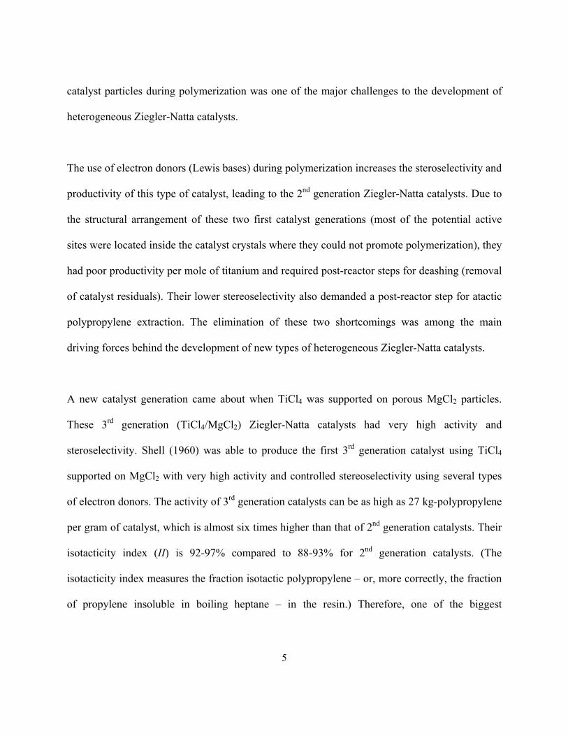
Electron donors are supposed to control the TiCl4 distribution on the (100) and (110) faces of the

MgCl2 surface as illustrated in Figure 2-1 (Busico et al., 1985; Chadwick et al., 2001). Ti2Cl8

species coordinate with the (100) faces through dinuclear bonds to form the isospecific

polymerization sites, while the electron donor molecules tend to coordinate with the non-

8

stereospecific (more acidic) sites on the (110) faces. When aromatic monoesters and diesters are

used as internal donors, the addition of alkylaluminiums (alkylation) will result in the partial

removal of the internal donors; therefore, the use of external donors is essential to maintain the

high steroselectivity level of these catalysts. During catalyst preparation there is still a chance of

the internal donor to coordinate with the (100) face; but it has been reported that, in the case of

ethyl benzoate, TiCl4 is able to remove the donor from that stereospecific face (100) during the

titanation step (addition of TiCl4 during the activation step). However, when 1,3-diethers are

used as internal donors, they coordinate strongly with the (110) faces and cannot be removed by

alkylaluminiums (Barino and Scordamaglia, 1998). As a consequence, Ziegler-Natta catalysts

with excellent isospecificity are obtained with diether internal donors in the absence of external

donors.

100 face

Cl

110 face

Ti

100 face

Cl

100 face

Cl

110 face

Ti

110 face

Ti

Figure 2-1: Lateral faces of a TiCl4/MgCl2 Ziegler-Natta catalyst (Busico et al., 1985).

The microstructure of polypropylene chains can be classified (Chadwick et al., 1996) from a

regioregularity point of view as regioregular (regular 1,2 insertions) and regioirregular (random

1,2 and 2,1 insertions). These chains can also be classified as isotactic (with methyl groups

aligned selectively at one side of the plane) as shown in Figure 2-2, or atactic (with a random

9

placement of methyl groups on either side of the plane), as illustrated in Figure 2-3. Isotactic

regioregular chains are also called stereoregular chains, and atactic chains are called

stereoirregular chains. Other arrangements for isotactic and atactic regioirregular chains are

illustrated in Figure 2-4 and Figure 2-5.

In the following sections, we will discuss the effects of hydrogen and electron donor on the

stereo- and regioregularity of polypropylene chains.

Figure 2-2: Isotactic regioregular chain (stereospecific).

Figure 2-3: Atactic regioregular chain (stereoirregular).

Figure 2-4: Isotactic regioirregular chain.

10

Figure 2-5: Atactic regioirregular chain.

2.2 Hydrogen Effect

Hydrogen always acts as a chain transfer agent during olefin polymerization: when the hydrogen

concentration increases, the molecular weight of the polyolefin decreases. On the other hand, the

effect of hydrogen on catalyst activity during olefin polymerization is less predictable and varies

depending on the type of catalyst, monomer, and donor systems. For instance, hydrogen

generally reduces the polymerization rate of ethylene and increases the polymerization rate of

propylene when high-activity TiCl4/MgCl2 catalysts are used (Shaffer and Ray, 1996).

The initial rate of propylene polymerization increases when the partial pressure of hydrogen is

increased, which seems to indicate that the hydrogen activation process is very fast. Some

researchers have proposed that this polymerization rate increase was due to the ease access of

monomer to the catalyst active site since, in the presence of hydrogen, the molecular weight of

the polymer decreases and the monomer diffusion rate would be higher (Boucheron, 1975). This

is not true, however, in the case of ethylene, where the polymerization rate generally decreases

11

when hydrogen is introduced into the reactor. Other investigators have assumed that the decrease

in the overall polymerization rate is due to the decrease in the rate of reinitiation of metal-

hydride sites (Ti-H) formed after transfer to hydrogen (Natta, 1959; Soga and Sino, 1982).

It has also been reported (Chadwick et al., 1996) that the ratio of propagation rate to chain

transfer rate depends on the stereo- and regioregularity of the last monomer unit added to the

polymer chain in the order: stereoregular > stereoirregular > regioirregular.

Due to detection limitations of 13C NMR spectroscopy on regio-defects of highly isotactic

polypropylene, Busico et al. (1992) studied polypropylene samples of very small molecular

weight averages (propylene oligomers) by using excess hydrogen as the chain transfer agent. The

oligomers were characterized by chromatography/mass spectrometry (GC-MS). Monomer

insertions were classified as primary 1,2 (kpp = head-to-tail or ksp = head-to-head) or secondary

2,1 (kps = tail-to-tail or kss = tail-to-head), as shown in Schemes 2-1 and 2-2. Their experimental

results showed that the ratio of 1,2 to 2,1 insertions increased as the degree of polymerization

decreased, that is, shorter chains made at higher hydrogen concentrations had fewer 2,1

regioirregularities.

12

Ti CH2 CH

CH3

P + C3H6

kppTi CH2 CH

CH3

CH2 CH

CH3

P

Ti CH2CH

CH3

P + C3H6

kspTi CH2 CH

CH3

CH

CH3

PCH2

Scheme 2-1: 1,2 propylene insertion.

Ti CH2 CH

CH3

P + C3H6

kpsTi CH2CH

CH3

CH2 CH

CH3

P

Ti CH2CH

CH3

P + C3H6

kssTi CH2CH

CH3

CH

CH3

PCH2

Scheme 2-2: 2,1 propylene insertion.

The increase in propylene polymerization rate by addition of hydrogen is well known. In the

absence of hydrogen, regioirregular-terminated chains will be formed on some of the catalyst

sites. These sites are considered “dormant” because the regioirregular insertions at the chain end

slow down the next monomer insertion, thus reducing the overall propylene polymerization rate

(Rishina el al., 1994). When hydrogen is added to the reactor, it reacts with the “dormant” 2,1-

terminated chains, freeing up the sites for polymerization (Kissin and Rishina, 2002; Kissin et

al., 1999; Kissin et al., 2002). Busico et al. (1992) showed that the ratio of 1,2 to 2,1 insertions

increased (the chains became more regioregular) as the molecular weight decreased because

hydrogen will more likely terminate chains after a 2,1 insertion due to their lower rate of chain

13

growth. These conclusions have been supported by the analyses of Chadwick et al. (1994) for

chain-end determination. They showed that donors with a lower hydrogen activation effect

produced polypropylene with the lowest fraction of chain-ends formed by chain transfer after

2,1-insertion.

Guastalla and Giannini (1983) carried out some experiments measuring the effect of the initial

concentration of hydrogen on the polymerization rate measured after one minute of

polymerization. They showed that the propylene polymerization rate increased dramatically by

increasing the hydrogen concentration up to a certain maximum hydrogen partial pressure of

about 0.6 kg/cm2, after which no more rate effects were detected. They suggested that this

behaviour was caused by the adsorption of hydrogen on the catalyst surface, but did not provide

any further evidence to support their explanation.

Kissin and Rishina (2002) studied the effect of hydrogen concentration on propylene and

ethylene polymerization. They concluded that the existence of dormant or stable Ti-CH(R)CH3

sites (R is CH3 for propylene and H for ethylene polymerization) is the reason for the different

effect that hydrogen has on the polymerization rate of propylene and ethylene. Their explanation

for the effect of hydrogen on propylene polymerization coincides with the one proposed by

Busico et al (1992) discussed above. For the rate decrease effect of hydrogen on ethylene

polymerization, they proposed the formation of a dormant site with the general structure Ti-

CH2CH3. One of the hydrogen atoms bonded to the β carbon interacts with the vacancy on the

titanium atom (β-agostic interaction), slowing down monomer propagation. They argue that the

14

Ti-CH2CH3 is formed after ethylene insertion on a Ti-H site produced by transfer to hydrogen.

Consequently, as hydrogen concentration increases, the fraction of Ti-H sites and “dormant” Ti-

CH2CH3 species will also increase. One must be aware, however, that β-hydride elimination also

produces Ti-H sites and that transfer to ethylene will form Ti-CH2CH3 sites and, therefore, this

explanation is only strictly valid if the main transfer mechanism in the absence of hydrogen is

transfer to cocatalyst.

2.3 Stereoregularity

Understanding the geometry of Ziegler-Natta catalysts helps simplify the complexity of the

electron donor roles and explain the behavior of different active site types. As discussed above

(Busico et al., 1985; Barino and Scordamaglia, 1998; Chadwick et al., 2001), internal donors are

used to block non-stereoselective (110) catalyst faces on the catalyst. These internal donors

(aromatic monoesters or aromatic diesters) are partially lost during the alkylation process;

therefore, the use of external donors during the polymerization reaction is essential to maintain

high stereoselectivity of the catalysts to make highly isotactic polypropylene. Figure 2-6 shows a

molecular model for a TiCl4/MgCl2 catalyst used for propylene polymerization (Kakugo et al.,

1988). Three different site structures have been proposed: a highly isotactic, a low isotactic, and

an atactic site. The highly isotactic site has only one coordination vacancy and all its chlorine

atoms are bonded to magnesium atoms on the surface of the support. Despite of also having only

15

one coordination vacancy, two chlorine atoms of the low isotactic site are not bonded to a

magnesium atom, accounting for its lower isotacticity. Finally, the two coordination vacancies of

the atactic site allow for coordination of propylene in a random orientation, forming atactic

polypropylene chains.

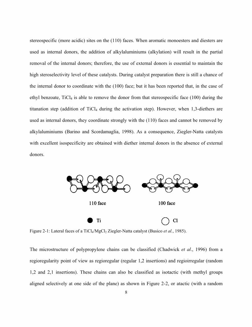
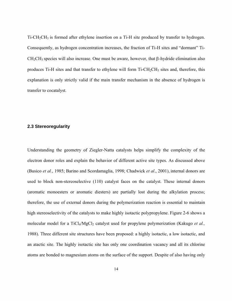
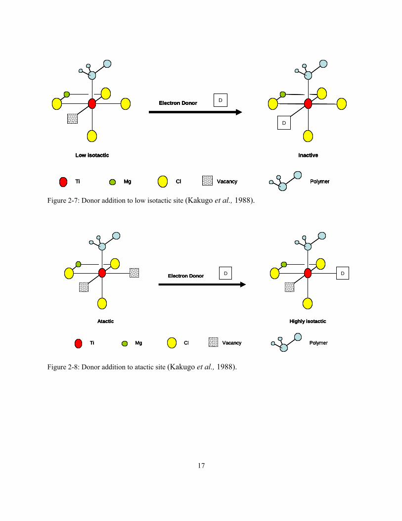
The addition of electron donors is explained in Figure 2-7 and Figure 2-8. When the electron

donor complexes with the low isotactic site, it blocks the coordination vacancy, rendering the site

inactive for polymerization. On the other hand, when the electron donor complexes with one of

the coordination vacancies of the atactic site, the site becomes isotactic, since only one

coordination vacancy (and, therefore, only one mode of monomer orientation) is left for

propylene polymerization. It is interesting to notice that some donors may completely kill the

catalyst when used in excess. This phenomenon is utilized in some commercial processes to kill

the polymerization (self extinction) during plant shutdowns. This procedure avoids

contaminating the reaction system with undesired poisons such as carbon monoxide. In this case,

the excess donor will block not only the coordination vacancies on the atactic and low isotactic

site, but also on the isotactic sites. However, not all donors act as catalyst poisons, even if an

excess is added to the polymerization reactor.

Busico et al. (1999) prefer to classify the catalyst sites as highly isotactic, poorly isotactic

(isotactoid), and syndiotactic. Atactic polypropylene is assumed to be produced in the poorly

isotactic and syndiotactic sites, due to the transformation of one site into the other. Figure 2-9

shows the three types of sites proposed by Busico. The highly isotactic site (a) has either two

16

ligands (a chlorine or a donor atom) or one ligand with a strong steric hindrance to prevent a

wrong insertion of monomer at position S2. The isotactoid site (b) has only one ligand. The

syndiotactic site (c) has two vacancies and no stereoselective control. Busico et al. have

proposed that the loss of steric hindrance may lead to the transformation of highly isotactic sites

to isotactoid and then to syndiotactic sites.

Ti PolymerVacancyMg Cl

Highly isotactic Low isotactic Atactic

D

Ti PolymerVacancyMg Cl

Highly isotactic Low isotactic Atactic

Ti PolymerVacancyMg ClTi PolymerVacancyMg Cl

Highly isotactic Low isotactic Atactic

DD

Figure 2-6: Catalyst site geometric models. D stands for the donor (Kakugo et al., 1988).

17

Ti PolymerVacancyMg Cl

Inactive Low isotactic

Electron Donor D

D

Ti PolymerVacancyMg Cl

Inactive Low isotactic

Electron Donor D

Ti PolymerVacancyMg Cl

Inactive Low isotactic

Ti PolymerVacancyMg ClTi PolymerVacancyMg Cl

Inactive Low isotactic

Electron Donor DElectron Donor D

DD

Figure 2-7: Donor addition to low isotactic site (Kakugo et al., 1988).

Electron Donor D

Atactic

Ti PolymerVacancyMg Cl

Highly isotactic

DElectron Donor DElectron Donor D

Atactic Atactic

Ti PolymerVacancyMg ClTi PolymerVacancyMg ClTi PolymerVacancyMg Cl

Highly isotactic

D

Highly isotactic

DD

Figure 2-8: Donor addition to atactic site (Kakugo et al., 1988).

18

S2

S1

L2

L1

S2

S1

S2

S1

( a ) ( c )( b )

S1, S2= Cl = Ti= Mg or Ti = Vacancy = L1, L2 = Legend Cl or Donor

S2

S1

L2

L1

S2

S1

S2

S1

( a ) ( c )( b )

S2

S1

L2

L1

S2

S1

S2

S1

S2

S1

L2

L1

S2

S1

L2

L1

S2

S1

S2

S1

S2

S1

S2

S1

( a ) ( c )( b )

S1, S2= Cl = Ti= Mg or Ti = Vacancy = L1, L2 = Legend Cl or Donor

Figure 2-9: Active species models: (a) highly isotactic (b) isotactoid (c) syndiotactic (Busico et al., 1999).

2.4 Regioregularity

Chain regioregularity has a significant effect on the properties of polypropylene. There are two

possible modes of propylene insertion: 1-2 or 2-1. Regioregular chains are composed of many 1-

2 or 2-1 insertions, without any insertion defects. For the coordination polymerization of

propylene, the most common insertion type is 1-2, since the methyl group “prefers” to be

positioned away from the active site due to steric hindrances. A 2-1 insertion after a 1-2 insertion

will cause a regioirregular sequence in the polymer chain. This irregularity will decrease the

melting temperature and crystallinity of the polymer.

19

For propylene made with MgCl2/TiCl4/diether system, there is a relation between chain transfer

by hydrogen and the type of insertion (Chadwick et al., 1996). Polypropylene chains terminated

with normal-butyl or iso-butyl groups result from transfer to hydrogen following 2-1 or 1-2

insertions, respectively. These chain transfer reactions depend on the components of the reaction

system (catalyst, cocatalyst, donor, and monomer) and on the hydrogen concentration (Chadwick

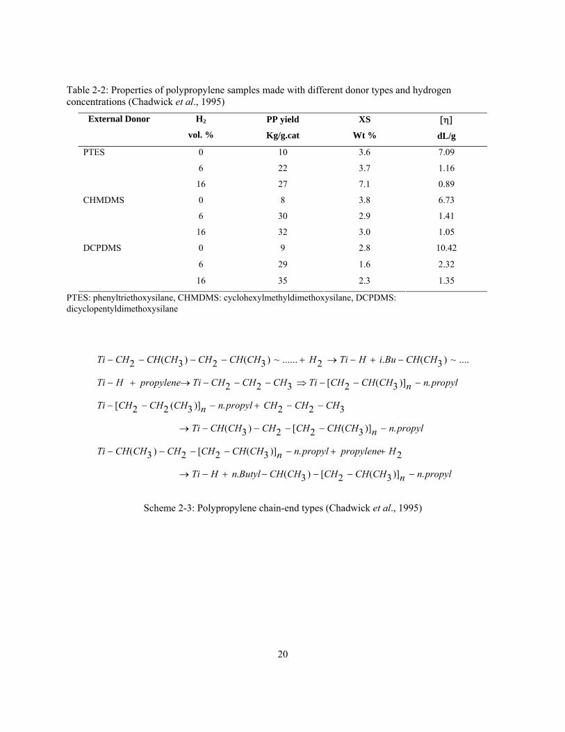
et al., 1995; Chadwick et al., 1996). Table 2-2 shows that polypropylene tacticity (as measured

by the fraction of polymer insoluble in boiling xylene, XS) depends on electron donor type and

hydrogen concentration. In their work, three different external donors were used with

MgCl2/TiCl4/DIBP catalyst: phenyltriethoxysilane (PTES), cyclohexylmethyldimethoxysilane

(CHMDMS), and dicyclopentyldimethoxysilane (DCPDMS). These three donors were chosen

because they produced catalyst systems with different hydrogen sensitivities on polymer

molecular weight. PTES shows the lowest and DCPDMS shows the highest hydrogen response.

Chadwick et al. (1995) reported that for CHMDMS and DCPDMS donors, propagation after 2-1

insertion could happen due the presence of regioirregular (head-to-head) sequences in the xylene

soluble fraction. However, no regioregularity was detected in the isotactic fraction. The chain-

end distribution of the isotactic fraction made with the three donors is shown in Table 2-3. The

three possible chain-end types are illustrated in Scheme 2-3. The fraction of n-Bu terminated

chains decreases when hydrogen concentration increases.

20

Table 2-2: Properties of polypropylene samples made with different donor types and hydrogen concentrations (Chadwick et al., 1995)

External Donor H2

vol. %

PP yield

Kg/g.cat

XS

Wt %

[η]

dL/g

0 10 3.6 7.09

6 22 3.7 1.16

PTES

16 27 7.1 0.89

0 8 3.8 6.73

6 30 2.9 1.41

CHMDMS

16 32 3.0 1.05

0 9 2.8 10.42

6 29 1.6 2.32

DCPDMS

16 35 2.3 1.35

PTES: phenyltriethoxysilane, CHMDMS: cyclohexylmethyldimethoxysilane, DCPDMS: dicyclopentyldimethoxysilane

propylnnCHCHCHCHCHButylnHTi

HpropylenepropylnnCHCHCHCHCHCHTi

propylnnCHCHCHCHCHCHTi

CHCHCHpropylnnCHCHCHTi

propylnnCHCHCHTiCHCHCHTipropyleneHTi

CHCHBuiHTiHCHCHCHCHCHCHTi

.)]3(2[)3(.

2 .)]3(2[2)3(

.)]3(2[2)3(

322 .)]3(22[

.)]3(2[322

....~)3(. 2 ......~)3(2)3(2

−−−−+−→

++−−−−−

−−−−−→

−−+−−−

−−−⇒−−−→+−

−+−→+−−−−

Scheme 2-3: Polypropylene chain-end types (Chadwick et al., 1995)

21

Table 2-3: Chain-end distribution in isotactic sample (Chadwick et al., 1995)

External donor H2 Chain-end distribution in %

vol. % n- propyl i- butyl n-butyl 6 50 31 19

PTES 16 50 41.5 8.5

6 50 27 23 CHMDMS

16 50 38 12

DCPDMS 16 50 33 17

However, it has been also reported by Chadwick et al. (1996) that for highly isotactic

polypropylene made with MgCl2/TiCl4/diether at low H2 concentration, the fraction of chains

with n-Bu chain ends was high. Therefore, they concluded that for the MgCl2/TiCl4/diether

system, highly stereospecific sites were not totally regiospecific, contrarily to their previous

investigation (Chadwick et al., 1995). This shows the danger of postulating general rules for

these complex catalyst/donor systems.

22

Chapter 3

Reaction Mechanism and Mathematical Modeling

3.1 Introduction

Mathematical models for olefin polymerization are useful to predict polymer microstructure and

properties in laboratory and industrial reactor scales. There are several methods for modeling

olefin polymerization reactors (Soares, 2001). Most of them start by defining the polymerization

mechanism and then setting up population balances for all the chemical species involved in the

polymerization. The dynamic solution of the complete population balances, to generate the

molecular weight distribution (MWD) of polyolefins, requires sophisticated ordinary differential

equation (ODE) solvers, since the set of population balance ODEs may involve thousands of

equations. A more common alternative is to use the method of moments to reduce the size of the

ODE system to just a few equations for the leading moments. These systems are much easier to

solve, but only some of the molecular weight averages can be predicted, not the complete MWD.

Finally, the method of instantaneous distributions uses closed analytical solutions for the

instantaneous MWD that can be integrated over time. This method requires the lowest

computation time and generates complete microstructural distributions but, unfortunately,

instantaneous distributions are not available for all polymerization mechanisms.

23

Monte Carlo simulation is also a very powerful modeling approach. It also starts by defining the

polymerization mechanism but, contrarily to the methods discussed in the previous paragraph,

there is no need to formulate population balances. The polymerization mechanism is used to

create an algorithm where polymer chains are generated one by one using a set of reaction

probabilities based on the polymerization kinetic constants. Monte Carlo simulation gives the

maximum amount of information on polymer microstructure but it is generally the most time

consuming technique of all discussed above.

The tacticity distribution of polypropylene resins is one of their most important properties.

However, no detailed mathematical model has been developed to date to describe the tacticity

distribution of polypropylene chains made with multiple-site catalysts. We may postulate the

existence of at least three types of active sites on Ziegler-Natta catalysts used for propylene

polymerization: sites that make only atactic chains, sites that only make isotactic chains, and

sites that may alternate between stereoselective and aspecific states. Based on the mechanistic

studies of Kakugo et al. (1988) and Busico et al. (1995, 1999) (See Figure 2-7 and Figure 2-8),

atactic sites can be reversibly converted to isotactic sites by complexation with an electron donor

molecule. Therefore, these sites could have two states: one atactic and one isotactic state. If this

conversion takes place during the lifetime of a polypropylene chain, stereoblock chains (atactic-

isotactic-atactic-isotactic-…) may be formed.

24

The active site type that can alternate between stereospecific and aspecific states can produce

three types of dead polymer chains: 1) purely isotactic chains are formed when they grow during

the stereospecific state and terminate before transformation to the atactic state, 2) purely atactic

chains are formed when they grow during the aspecific state and terminate before transformation

to the stereospecific state, and 3) stereoblock chains are formed when the site state changes from

stereospecific to aspecific and/or vice-versa during the life time of the chain. Stereoblock chains

can be further subdivided into diblock, triblock, tetrablock, and higher multiblock chains as

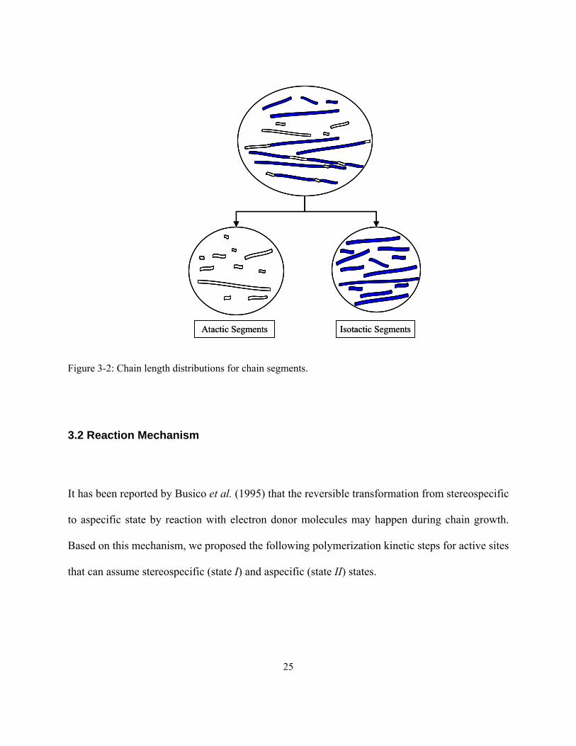
presented in Figure 3-1. On the other hand and in order to overview the entire population of the

polymer chains, they were classified based on the segment type as illustrated in Figure 3-2.

StereoblocksPure AtacticPure Isotactic

2 Blocks

4 Blocks

5 Blocks

3 Blocks

StereoblocksPure AtacticPure Isotactic

2 Blocks

4 Blocks

5 Blocks

3 Blocks

Figure 3-1: Chain populations with different number of stereoblocks. (Whole chains.)

25

Atactic Segments Isotactic SegmentsAtactic Segments Isotactic Segments

Figure 3-2: Chain length distributions for chain segments.

3.2 Reaction Mechanism

It has been reported by Busico et al. (1995) that the reversible transformation from stereospecific

to aspecific state by reaction with electron donor molecules may happen during chain growth.

Based on this mechanism, we proposed the following polymerization kinetic steps for active sites

that can assume stereospecific (state I) and aspecific (state II) states.

26

Activation

Catalyst (CI and CII) at state I or II is activated (alkylated and reduced) by reaction with

alkylaluminum cocatalysts (Al) according to Equations (3-1) and (3-2), forming monomer-free

active sites, IP0 and IIP0 , where the subscript “0” indicates that there are no monomer units

attached to the active site:

IaI PkAlC 0

1⎯⎯→⎯+ ( 3-1)

IIaII PkAlC 0

2⎯⎯ →⎯+ ( 3-2)

Passivation

Alkylaluminum molecules (such as triethylaluminum TEA) can also act as scavengers by

reacting with polar molecules such as water or oxygen (I) present in the system in trace amounts,

according to the reaction:

IAlkIAl IAl ⋅⎯⎯ →⎯+ ⋅ ( 3-3)

27

Initiation

Monomer-free sites, either resulting from catalyst activation ( IP0 , IIP0 ) or chain transfer reactions

( IHP , II

HP , IEtP , II

EtP ), are initiated by insertion of the first monomeric unit (M) according to the

following elementary steps:

IiI PkMP 1,11

0 ⎯→⎯+ ( 3-4)

IIiII PkMP 1,12

0 ⎯⎯→⎯+ ( 3-5)

IiHIH PkMP 1,1

1⎯⎯ →⎯+ ( 3-6)

IIiHIIH PkMP 1,1

2⎯⎯ →⎯+ ( 3-7)

IiRIEt PkMP 1,1

1⎯⎯ →⎯+ ( 3-8)

IIiRIIEt PkMP 1,1

2⎯⎯ →⎯+ ( 3-9)

Notice that we adopted the following convention to keep track of polymer chain length, number

of blocks per chain, and catalyst state: stateblocksofnumberlengthchainP ,

Site Transformation by Electron Donor

The most important innovation in the mathematical model proposed in this thesis is modeling of

the reversible site transformation from the stereospecific state I to the aspecific state II in the

presence of the electron donor (Do). As the site state changes from II to I (by coordination with

28

an electron donor molecule) or from I to II (by release of an electron donor molecule), the

polymer chain length is not altered (r remains the same), but the number of stereoblocks

increases by 1 (i+1), as shown in the equations below:

IkII PDoP Do00 ⎯→⎯+

+

( 3-10)

DoPP IIkI Do +⎯→⎯−

00 ( 3-11)

IH

kIIH PDoP Do⎯→⎯+

+

( 3-12)

DoPP IIH

kIH

Do +⎯→⎯−

( 3-13)

IEt

kIIEt PDoP Do⎯→⎯+

+

( 3-14)

DoPP IIEt

kIEt

Do +⎯→⎯−

( 3-15)

Iir

kIIir PDoP Do

1,, +⎯→⎯++

( 3-16)

DoPP IIir

kIir

Do +⎯→⎯ +

−

1,, ( 3-17)

Equations (3-16) and (3-17) keep track of the number of blocks and chain length of the whole

polymer chain. However, it is also useful to find out the distribution of sizes of isotactic (I) and

atactic (II) blocks. For this distribution, we have to reformulate our equations so that we describe

the concentration of blocks of length r ( IrB and II

rB ), according to the equations:

Ii

IIr

kIIir PBDoP Do

1,0, ++⎯→⎯++

( 3-18)

29

DoPBP IIi

Ir

kIir

Do ++⎯→⎯ +

−

1,0, ( 3-19)

Notice that, after a site transformation step, the length of the living polymer is reset to zero, since

a new block starts forming at this moment. With these expressions, we are able to follow the

length of all isotactic and atactic segments in the reactor without considering the particular chain

(isotactic, atactic, stereoblock) they belong to.

Propagation

Propagation is the most common step during polymerization. The addition of monomer to sites

in state I or II increases the length of the chain by one unit (r+1), as indicated below:

Iir

kIir PMP p

,1,1

+⎯→⎯+ ( 3-20)

IIir

kIIir PMP p

,1,2

+⎯→⎯+ ( 3-21)

Although there could be four different types of regio insertions (head-to-head, head-to-tail, tail-

to-head, and tail-to-tail) leading to four different propagation constants, we will not distinguish

between them in this model.

30

Chain Transfer

The five most common chain transfer steps in coordination polymerization are β-hydride-

elimination, β-methyl-elimination, transfer to hydrogen, transfer to monomer, and transfer to

cocatalyst. These chain transfer steps are described in more details below.

β-hydride elimination: During β-hydride elimination, one of the hydrogen atoms attached to the

β carbon atom is transferred to the titanium active site, forming a metal hydride Ti-H site ( IHP or

IIHP ) and a dead chain with a terminal unsaturated ( I

irD , or IIirD , ).

Iir

IH

kIir DPP ,,

1 +⎯→⎯ β ( 3-22)

IIir

IIH

kIIir DPP ,,

2 +⎯→⎯ β ( 3-23)

β-methyl elimination: During β-methyl elimination, the methyl group attached to the β carbon

atom is transferred to the titanium active site, forming a metal methyl Ti-CH3 site and a dead

polypropylene with terminal vinyl group. This transfer step may be important for some

metallocene catalyst but happens rarely with Ziegler Natta catalyst and will not be included in

this model.

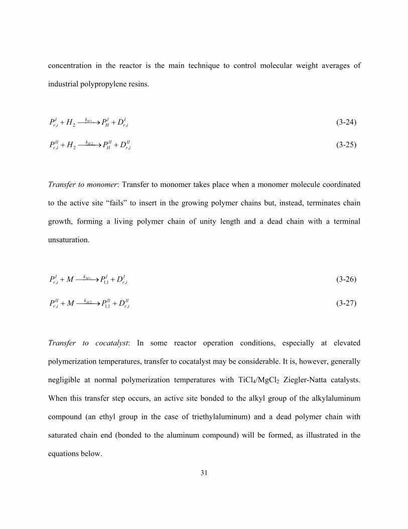
Transfer to hydrogen: The main transfer step in industrial-scale propylene polymerization is

transfer to hydrogen. This transfer step will also generate a metal hydride Ti-H site, as for β-

hydride elimination, but the dead chain will have a saturated chain end. Varying hydrogen

31

concentration in the reactor is the main technique to control molecular weight averages of

industrial polypropylene resins.

Iir

IH

kIir DPHP H

,2,1 +⎯→⎯+ ( 3-24)

IIir

IIH

kIIir DPHP H

,2,2 +⎯⎯→⎯+ ( 3-25)

Transfer to monomer: Transfer to monomer takes place when a monomer molecule coordinated

to the active site “fails” to insert in the growing polymer chains but, instead, terminates chain

growth, forming a living polymer chain of unity length and a dead chain with a terminal

unsaturation.

Iir

IkIir DPMP M

,1,1,1 +⎯→⎯+ ( 3-26)

IIir

IIkIIir DPMP M

,1,1,2 +⎯⎯→⎯+ ( 3-27)

Transfer to cocatalyst: In some reactor operation conditions, especially at elevated

polymerization temperatures, transfer to cocatalyst may be considerable. It is, however, generally

negligible at normal polymerization temperatures with TiCl4/MgCl2 Ziegler-Natta catalysts.

When this transfer step occurs, an active site bonded to the alkyl group of the alkylaluminum

compound (an ethyl group in the case of triethylaluminum) and a dead polymer chain with

saturated chain end (bonded to the aluminum compound) will be formed, as illustrated in the

equations below.

32

Iir

IEt

kIir DPAlP Al

,,1 +⎯⎯→⎯+ ( 3-28)

IIir

IIEt

kIIir DPAlP Al

,,2 +⎯⎯ →⎯+ ( 3-29)

Site Deactivation

Most Ziegler-Natta catalysts deactivate according to first or second order kinetics, generating a

dead polymer chain and a deactivated site (Cd) that is unable to catalyze polymerization. We

have adopted the first order deactivation kinetics for simplicity in this model.

Iird

kIir DCP d

,,1 +⎯→⎯ ( 3-30)

IIird

kIIir DCP d

,,2 +⎯→⎯ ( 3-31)

Catalyst Poisoning

The existence of catalyst poisons in the polymerization system is considered one of the worst

conditions in industrial polymerization processes. One of the functions of alkylaluminum

catalysts is to passivate the system by removing most of the polar poisons in the reactor prior to

catalyst injection and polymerization. Catalyst poisoning will result in an inactive catalyst and a

dead polymer chain. Even though the kinetics of catalyst poisoning is not well understood, we

have adopted the simple bimolecular mechanism shown below to describe a generic poisoning

step with a polar impurity (I):

33

Iird

kIir DCIP dI

,,1 +⎯⎯→⎯+ ( 3-32)

IIird

kIIir DCIP dI

,,2 +⎯⎯→⎯+ ( 3-33)

3.3 Mathematical Modeling of Olefin Polymerization in Continuous Stirred Tank

Reactors

The proposed model can describe the MWD and molecular weight averages of purely isotactic,

purely atactic, and stereoblock chains, as illustrated in Figure 3-1. The model can also describe

the MWD and molecular weight averages of isotactic and atactic segments, as shown in Figure

3-2. These two approaches permit a very detailed description of the polymer microstructure, as

will be demonstrated below.

We formulated three types of population balances, to monitor different aspects of the

polypropylene chain microstructures:

1) Balances for the whole chains, without monitoring the number or type of stereoblocks

per chain (Section 3.3.1)

2) Balances for purely isotactic, purely atactic, and stereoblock chains (Section 3.3.2)

3) Balances for chain segments (Section 3.3.3)

34

Since these population balances are difficult to solve, we will also formulate the moment

equations for each population balance (Sections 3.3.4 to 3.3.6).

The balances derived in this chapter describe only the polymerization taking place in active sites

that can undergo the stereospecific-aspecific transition discussed above. Active sites that produce

only isotactic or atactic chains are much easier to model, since their behavior is a particular

solution (when no site transition takes place) of the general model derived herein.

The following lumped kinetic constants will be used in our derivation to reduce the size of the

resulting population balance and moment equations:

AlkHkMkkK AlHMT 121111 +++= β ( 3-34)

AlkHkkK AlHT 1211'

1 ++= β ( 3-35)

IkkK dIdD 111 += ( 3-36)

AlkHkMkkK AlHMT 222222 +++= β ( 3-37)

AlkHkkK AlHT 2222'

2 ++= β ( 3-38)

IkkK dIdD 222 += ( 3-39)

By inspection of the polymerization mechanism shown in Equations (3-1) to (3-33), the

following molar balances can be written for monomer-free active sites in a continuous stirred-

tank reactor (CSTR)

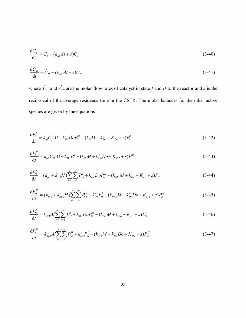
35

IaII CsAlkC

tC )(ˆd

d1 +−= ( 3-40)

IIaIIII CsAlkCt

C)(ˆ

dd

2 +−= ( 3-41)

where IC and IIC are the molar flow rates of catalyst in state I and II to the reactor and s is the

reciprocal of the average residence time in the CSTR. The molar balances for the other active

species are given by the equations

IDDoi

IIDoIa

I

PsKkMkDoPkAlCkt

P01101

0 )(d

d+++−+= −+ ( 3-42)

IIDDoi

IDoIIa

II

PsKDokMkPkAlCkt

P02202

0 )(d

d+++−+= +− ( 3-43)

IHDDoiH

IIHDo

i r

IirH

IH PsKkMkDoPkPHkkt

P )()(d

d11

1 1,11 +++−++= −+

∞

=

∞

=∑∑β ( 3-44)

IIHDDoiH

IHDo

i r

IIirtHt

IIH PsKDokMkPkPHkkt

P )()(d

d22

1 1,22 +++−++= +−

∞

=

∞

=∑∑β ( 3-45)

IEtDDoiR

IIEtDo

i r

IirAl

IEt PsKkMkDoPkPAlkt

P )(d

d11

1 1,1 +++−+= −+

∞

=

∞

=∑∑ ( 3-46)

IIEtDDoiR

IEtDo

i r

IIirAl

IIEt PsKDokMkPkPAlkt

P )(d

d22

1 1,2 +++−+= +−

∞

=

∞

=∑∑ ( 3-47)

36

3.3.1 Population Balances for Whole Chains

The population balance for living chains with length r = 1 growing on a site at state I is given by

IDTDo

Ip

IIDo

r

IrM

IEtiR

IHiH

Ii

I

PsKKkMPkDoPkPMk

MPkPkPkt

P

1111111

1

11011

)(

)(d

d

+++−−++

++=

−+∞

=∑

( 3-48)

Notice that the subscript i, used to count the number of blocks in the chain ( IirP , ), is not required

in this balance and was removed to simplify the notation.

For living chains with lengths greater than 1, r ≥ 2, the equivalent population balance is

IrDTDo

Irp

IIrDo

Irp

Ir PsKKkMPkDoPkMPkt

P )(d

d11111 +++−−+= −+

− ( 3-49)

Similarly, the population balance for living chains with length r = 1 at state II is

IIDTDo

IIp

IDo

r

IIrM

IIEtiR

IIHiH

IIi

II

PsKKDokMPkPk

PMkMPkPkPkt

P

122121

122202

1

)(

)(d

d

+++−−+

+++=

+−

∞

=∑ ( 3-50)

37

and, for living chains with r ≥ 2 at state II

IIrDTDo

IIrp

IrDo

IIrp

IIr PsKKDokMPkPkMPkt

P )(d

d22212 +++−−+= +−

− ( 3-51)

Population balances for dead chains are also easily formulated as follow

Ir

IrDT

Ir sDPKK

tD

−+= )(d

d11 ( 3-52)

IIr

IIrDT

IIr sDPKKt

D−+= )(

dd

22 ( 3-53)

3.3.2 Population Balances for Isotactic, Atactic and Stereoblock Chains

Isotactic Chains

Purely isotactic living chains are those growing on sites at state I with only one block (i=1). If

the site state changes to II, the chain is reclassified as stereoblock, as described below. The

population balances for these chains are given by the expressions

38

IDTDo

Ip

r

IrM

IEtiR

IHiH

Ii

I

PsKKkMPk

PMkMPkPkPkt

P

1,1111,11

111101

1,1

)(

)(d

d

+++−−

+++=

−

∞

=∑ ( 3-54)

IrDTDo

Ir

Irp

Ir PsKKkPPMkt

P1,111,1,11

1, )()(d

d+++−−= −

− ( 3-55)

Atactic Chains

Similarly, purely atactic living chains are those growing on a site at state II with only one block

(i=1). Their population balances are expressed as follows:

IIDTDo

IIp

r

IIrM

IIEtiR

IIHiH

IIi

II

PsKKDokMPk

PMkMPkPkPkt

P

1,1221,12

122202

1,1

)(

)(d

d

+++−−

+++=

+

∞

=∑ ( 3-56)

IIrDTDo

IIr

IIrp

IIr PsKKDokPPMkt

P1,221,1,12

1, )()(d

d+++−−= +

− ( 3-57)

Stereoblock Chains

Stereoblock chains have two or more blocks, i ≥ 2, and are formed when the site state changes

from aspecific to stereospecific or vice-versa. Their population balances are also easily derived

from the polymerization mechanism adopted in the model:

IirDTDo

IIirDo

Iir

Iirp

Iir PsKKkDoPkPPMk

tP

,111,,,11, )()(

dd

+++−+−= −−

+− ( 3-58)

39

IIirDTDo

IirDo

IIir

IIirp

IIir PsKKDokPkPPMk

tP

,221,,,12, )()(

dd

+++−+−= +−

−− ( 3-59)

Population balances for the equivalent dead polymer chains are

Ir

IrDT

Ir sDPKKt 1,1,11

1, )(d

dD−+= ( 3-60)

IIr

IIrDT

IIr sDPKKt

D1,1,11

1, )(d

d−+= ( 3-61)

Iir

IirDT

Iir sDPKK

t ,,11, )(

ddD

−+= ( 3-62)

IIir

IIirDT

IIir sDPKK

tD

,,11, )(

dd

−+= ( 3-63)

3.3.3 Population Balances for Chain Segments

Chain segments are denoted as IrB or II

rB . Purely isotactic or atactic chains are counted as one

segment. Population balances for chains segments are listed below. The only difference between

these moment equations and the ones derived in the previous section for isotactic, atactic, and

stereoblock chains is that the state transformation reaction is treated as a pseudo-transfer

reaction, zeroing the length of the chain and starting a new segment of different stereoregularity.

40

Isotactic Segments

IrDTDo

Ir

Irp

Ir BsKKkBBMkt

B )()(d

d1111 +++−−= −

− ( 3-64)

IDTDo

Ip

Ii

I

BsKKkMBkMBkt

B11

'11101

1 )(d

d+++−−= − ( 3-65)

IDDo

Ii

r

IrT

r

IIrDo

IIDoIa

I

BsKkMBkBKBDokDoBkAlCkt

B0101

1

'1

101

0 )(d

d++−−+++= −

∞

=

∞

=

++ ∑∑ ( 3-66)

Atactic Segments

IIrDTDo

IIr

IIrp

IIr BsKKDokBBMkt

B )()(d

d1112 +++−−= +

− ( 3-67)

IIDTDo

IIp

IIi

II

BsKKDokMBkMBkt

B11

'11202

1 )(d

d+++−+= + ( 3-68)

IIDDo

IIi

r

IIrT

r

IrDo

IDoIIa

II

BsKDokMBkBKBkBkAlCkt

B0202

1

'2

102

0 )(d

d++−−+++= +

∞

=

∞

=

−− ∑∑ ( 3-69)

3.3.4 Moments Equations for Whole Chains

The population balances developed in Sections 3.3.1 and 3.3.3 encompass thousands of

equations, one for each polymer of a given chain length r. Even though mathematical methods

exist to solve these very large systems of differential equations, it is much easier to apply the

41

method of moments to reduce the number of equations required in the simulation. The moments

of the living and dead chains for the whole chains are defined by Equations (3-70) and (3-71),

respectively, where j = I or II (site state), and m is the moment order:

∑∞

=

=1r

jr

mmj PrY ( 3-70)

∑∞

=

=1r

jr

mmj DrX ( 3-71)

The zeroth moment, defined when m = 0, measures the total number of polymer moles in a given

population. The first moment, m = 1, is the total mass of the polymer population. Finally, the

second moment, m = 2, does not have physical meaning but is required to calculate the weight

average molecular weight.

The method of moments can be used to estimate the number (Mn) and weight (Mw) average

molecular weights of the polymer populations with the following equations:

0000

1111

1

1 ..IIIIII

IIIIII

r r

r rn YXYX

YXYXmw

N

rNmwM

++++++

==∑∑

∞

=

∞

= ( 3-72)

1111

2222

1

12

..IIIIII

IIIIII

r r

r rw YXYX

YXYXmw

rN

NrmwM

++++++

==∑∑

∞

=

∞

= ( 3-73)

42

where mw is the molar mass of the repeating unit (mw = 42 g/mol for propylene).

Finally, the polydispersity index is easily calculated as

n

w

MM

PDI = ( 3-74)

Using the definition for the zeroth moment of living polymer, and also ignoring the number of

blocks per chain for the whole chains equations, Equations (3-44) and (3-46) can be rewritten as

IHDDoiH

IIHDoIH

IH PsKkMkDoPkYHkkt

P )()(d

d11

011 +++−++= −+

β ( 3-75)

IEtDDoiR

IIEtDoAl

IEt PsKkMkDoPkAlYkt

P )(d

d11

011 +++−+= −+ ( 3-76)

By substituting Equations (3-48) and (3-49) into Equation (3-70) and summing over all r values,

we obtain the moments of the living chains at state I for the whole chains:

43

01

'1

01101

0

)(

)(d

d

IDTDo

IIDoI

EtiRI

HiHI

iI

YsKKk

DoYkMPkPkPkt

Y

+++−

+++=

−

+

( 3-77)

11

'1

1011101

1

)(

)(d

d

IDTDo

IIDoIpI

EtiRI

HiHI

iI

YsKKk

DoYkMYkMPkPkPkt

Y

+++−

++++=

−

+

( 3-78)

21

'1

20111101

2

)(

)2()(d

d

IDTDo

IIDoIIpI

EtiRI

HiHI

iI

YsKKk

DoYkYYMkMPkPkPkt

Y

+++−

+++++=

−

+

( 3-79)

Similarly, moment equations for dead polymers are derived by substituting Equations (3-52) and

(3-70) into Equation (3-71) and summing over all r values:

0011

0

)(d

dIIDT

I sXYKKt

X−+= ( 3-80)

1111

1

)(d

dIIDT

I sXYKKt

X−+= ( 3-81)

2211

2

)(d

dIIDT

I sXYKKt

X−+= ( 3-82)

Moment equations for chains growing on sites at state II are derived in an analogous way and are

listed below:

02

'2

02202

0

)(

)(d

d

IDTDo

IDoII

EtiRII

HiHII

iII

YsKKDok

YkMPkPkPkt

Y

+++−

+++=

+

−

( 3-83)

44

12

'2

1022202

1

)(

)(d

d

IIDTDo

IDoIIpII

EtiRII

HiHII

iII

YsKKDok

YkMYkMPkPkPkt

Y

+++−

++++=

+

−

( 3-84)

22

'2

20112202

2

)(

)2()(d

d

IIDTDo

IDoIIIIpII

EtiRII

HiHII

iII

YsKKDok

YkYYMkMPkPkPkt

Y

+++−

+++++=

+

−

( 3-85)

0022

0

)(d

dIIIIDT

II sXYKKt

X−+= ( 3-86)

1122

1

)(d

dIIIIDT

II sXYKKt

X−+= ( 3-87)

2222

2

)(d

dIIIIDT

II sXYKKt

X−+= ( 3-88)

3.3.5 Moments Equations for Isotactic, Atactic and Stereoblock Chains

Isotactic Chains

Isotactic chains are those that propagate and terminate at state I, without transformation to state

II; therefore, all chains at state I and with i = 1 are pure isotactic chains.

The moment equations for isotactic living chains were obtained by substituting Equation (3-54)

and (3-55) in Equation (3-70) and summing over r.

45

01,11

011101

01,

)(

)(d

d

IDTDo

IMI

EtiRI

HiHI

iI

YsKKk

MYkMPkPkPkt

Y

+++−

+++=

−

( 3-89)

11,11

11

01,11101

11,

)(

)(d

d

IDTDo

IMIpI

EtiRI

HiHI

iI

YsKKk

MYkMYkMPkPkPkt

Y

+++−

++++=

−

( 3-90)

21,11

21

01,

11,11101

21,

)(

)2()(d

d

IDTDo

IMIIpI

EtiRI

HiHI

iI

YsKKk

MYkYYMkMPkPkPkt

Y

+++−

+++++=

−

( 3-91)

Similarly, moment equations for dead isotactic chains are given by the expressions:

01,

01,11

01, )(

dd

IIDTI sXYKKt

X−+= ( 3-92)

11,

11,11

11, )(

dd

IIDTI sXYKKt

X−+= ( 3-93)

21,

21,11

21, )(

dd

IIDTI sXYKKt

X−+= ( 3-94)

46

The number and weight average molecular weights (Mn and Mw) are calculated using expressions

similar to Equations (3-72) and (3-73). Moreover, the molar and mass fractions of isotactic

chains can be calculated with the following equations:

100% mole isotacticPurely 0000

01,

01, ×

+++

+=

IIIIII

II

YXYXYX

( 3-95)

100% mass isotacticPurely 1111

11,

11, ×

+++

+=

IIIIII

II

YXYXYX

( 3-96)

where the moments for the whole chains, shown in the denominator of Equations (3-95) and (3-

96), are calculated as indicated in Section 3.3.4.

Atactic Chains

Contrarily to the isotactic chains, the atactic chains are those that propagate and terminate at state

II without transformation to state I; therefore, all chains at state II with i = 1 are purely atactic

chains. By substituting Equation (3-56) and (3-57) in Equation (3-70) and summing over all r

values, the moment equations for the atactic chains were obtained as

47

01,22

022202

01, )()(

dd

IIDTDoIIMII

EtiRII

HiHII

iII YsKKDokMYkMPkPkPkt

Y+++−+++= + ( 3-97)

11,22

12

01,22202

11,

)(

)(d

d

IIDTDo

IIMIIpII

EtiRII

HiHII

iII

YsKKDok

MYkMYkMPkPkPkt

Y

+++−

++++=

+

( 3-98)

21,22

22

01,

11,22202

21,

)(

)2()(d

d

IIDTDo

IIMIIIIpII

EtiRII

HiHII

iII

YsKKDok

MYkYYMkMPkPkPkt

Y

+++−

+++++=

+

( 3-99)

01,

01,22

01, )(

dd

IIIIDTII sXYKKt

X−+= ( 3-100)

11,

11,22

11, )(

dd

IIIIDTII sXYKKt

X−+= ( 3-101)

21,

21,22

21, )(

dd

IIIIDTII sXYKKt

X−+= ( 3-102)

The number and weight average molecular weights (Mn and Mw) and the mole and mass percent

of atactic chains in the polymer were calculated using expressions similar to Equations (3-72),

(3-73), (3-95), and (3-96).

Stereoblock Chains

Moment equations for stereoblock chains are derived in a way similar to the one applied for

isotactic and atactic chains. The final moment equations for stereoblock chains terminating at

state I and with ith blocks are listed below.

48

0,11

01,

0, )(

dd

iIDTDoiIIDoiI YsKKkDoYk

tY

+++−= −−

+ ( 3-103)

1,11

11,

0,1

1, )(

dd

iIDTDoiIIDoiIpiI YsKKkDoYkMYk

tY

+++−+= −−

+ ( 3-104)

2,11

21,

0,

1,1

2, )()2(

dd

iIDTDoiIIDoiIiIpiI YsKKkDoYkYYMk

tY

+++−++= −−

+ ( 3-105)

0,

0,11

0, )(

dd

iIiIDTiI sXYKK

tX

−+= ( 3-106)

1,

1,11

1, )(

dd

iIiIDTiI sXYKK

tX

−+= ( 3-107)

2,

2,11

2, )(

dd

iIiIDTiI sXYKK

tX

−+= ( 3-108)

Similarly, the moment equations for stereoblock chains terminating at state II and with ith blocks

are:

0,22

01,

0, )(

dd

iIDTDoiIDoiII YsKKDokYk

tY

+++−= +−

− ( 3-109)

1,2

'2

11,

0,2

1, )(

dd

iIIDTDoiIDoiIIpiII YsKKDokYkMYk

tY

+++−+= +−

− ( 3-110)

2,2

'2

21,

0,

1,2

2, )()2(

dd

iIIDTDoiIDoiIIiIIpiII YsKKDokYkYYMk

tY

+++−++= +−

− ( 3-111)

0,

0,22

0, )(

dd

iIIiIIDTiII sXYKK

tX

−+= ( 3-112)

49

1,

1,22

1, )(

dd

iIIiIIDTiII sXYKK

tX

−+= ( 3-113)

2,

2,22

2, )(

dd

iIIiIIDTiII sXYKK

tX

−+= ( 3-114)

3.3.6 Moments Equation for Chain Segments

Moment equations for chain segments were derived in a similar way, using the population

balances given by Equations (3-64) to (3-69). Only their final expressions will be presented

below.

50

The moments for the isotactic or atactic (j = I or II) segments are defined as follows,

∑∞

=

=1r

jr

mmj BrW ( 3-115)

Isotactic Segments

0111101

0

)(d

dIDTDo

IM

Ii

I WsKKkMBkMBkt

W+++−+= − ( 3-116)

111

011101

1

)(d

dIDTDoIp

IM

Ii

I WsKKkMWkMBkMBkt

W+++−++= − ( 3-117)

211

0111101

2

)()2(d

dIDTDoIIp

IM

Ii

I WsKKkWWMkMBkMBkt

W+++−+++= − ( 3-118)

Therefore, the number average molecular weight of the isotactic segments can be calculated as

follows,

0

1

.I

IIn W

WmwM = ( 3-119)

and the weight average molecular weight of these isotactic segments can be also calculated as follows:

1

2

.I

IIw W

WmwM = ( 3-120)

Consequently the polydispersity is simply:

51

In

IwI

s MM

PDI = ( 3-121)

Atactic Segments

0221202

0

)(d

dIIDTDo

IIM

IIi

II WsKKDokMBkMBkt

W+++−+= + ( 3-122)

122

021202

1

)(d

dIIDTDoIIp

IIM

IIi

II WsKKDokMWkMBkMBkt

W+++−++= + ( 3-123)

222

0121202

2

)()2(d

dIIDTDoIIIIp

IIM

IIi

II WsKKDokWWMkMBkMBkt

W+++−+++= + ( 3-124)

The number and weight average molecular weights of the atactic segments are calculated with

equations analogous to the ones used for the isotactic segments.

52

Chapter 4 Steady-State and Dynamic CSTR Simulations

4.1 Simulation Methodology

The differential equations derived in Chapter 3 will be used in the steady-state and dynamic

simulations of propylene polymerization in this chapter.

The steady-state solution for a single-site catalyst (assuming states I or II) was derived and used

to simulate the polymerization of propylene in a CSTR at different operating conditions. The

effect of donor, hydrogen, and monomer concentrations on polypropylene microstructure were

investigated. Moreover, the effect of changing the values of some kinetic parameters on the

microstructure of polypropylene was also studied. The model was then extended to include a

total of four sites types, which represent the situation more commonly encountered with

heterogeneous Ziegler-Natta catalysts.

We have also simulated the dynamic behavior propylene polymerization in a CSTR with a

single-site and a four-site type catalyst. Similarly to what was done for the steady-state

simulations, we tested the model response to changes in reactant concentrations and kinetic

parameter values.

53

Table 4-1 lists the concentrations of catalyst, cocatalyst, electron donor, propylene and other

reagents under the reference simulation conditions. Table 4-2 lists the reference values for the

reaction kinetic rate constants used in the simulations. Unless otherwise stated, these were the

conditions used in all simulations.

Table 4-1: Reference polymerization conditions. mol/L mol/L

CI 0.00001 Al 0.0007

CII 0.00001 I 0

M 0.20 H2 0.004

Do 0.0007

Table 4-2: Reference reaction rate constants (j = 1, or 2 for rate constants or j = I or II for site states).

Constant (L/mol·s) Constant (L/mol·s) Constant (s-1)

kaj 3,000 kDo+ 150 kDo¯ 0.01

kij 3,000 kAlj 0 kβj 0

kpj 3,000 kAl·I 10,000 kdj 0.001

kHj 110 kMj 0

kdIj 8,000

The several rates of elementary reactions taking place during polymerization are defined with the

equations

54

jrpjpj MPkR = ( 4-1)

jrDjTjtrj PKKR )( += ( 4-2)

IrDotf PkR −=1 ( 4-3)

IIrDotf DoPkR +=2 ( 4-4)

where Rp is the rate of propagation, Rtr is the overall chain transfer rate, Rtf1 is rate of site

transformation of state I to II, Rtf2 is the rate of site transformation from state II to I, and j = 1, or

2 for rate constants or j = I or II for site states.

4.2 Steady-State Simulation

The dynamic equations derived for a CSTR in the previous chapter can be solved analytically

under steady-state conditions, as will be shown below. In order reduce the size of the resulting

set of equations, we defined the following lumped-parameter constants:

sKk DDo ++= −11α ( 4-5)

sKDok DDo ++= +22α ( 4-6)

AlkK aA 11 = ( 4-7)

AlkK aA 22 = ( 4-8)

55

sKKkDok

DTDo

Do

+++= −

+

111β ( 4-9)

sKKkDok

DTDo

Do

+++= −

+

1'1

'1β ( 4-10)

sKKDokk

DTDo

Do

+++= +

−

222β ( 4-11)

sKKDokk

DTDo

Do

+++= +

−

2'

2

'2β ( 4-12)

sKKkk

DTDo

p

+++= −

11

11δ ( 4-13)

sKKkk

DTDo

p

+++= −

1'1

1'1δ ( 4-14)

sKKkk

DTDo

M

+++= −

11

1''1δ ( 4-15)

sKKDokk

DTDo

p

+++= +

22

22δ ( 4-16)

56

sKKDokk

DTDo

p

+++= +

2'

2

2'2δ ( 4-17)

sKKDokk

DTDo

M

+++= +

22

2''2δ ( 4-18)

)()(

11

11011 sKKk

PkPkPk

DTDo

IEtiR

IHiH

Ii

+++++

= −γ ( 4-19)

sKKkPkPkPk

DTDo

IEtiR

IHiH

Ii

+++++

= −1

'1

1101'1γ ( 4-20)

sKKkBkBkDTDo

IM

Ii

++++

= −11

1101''1γ ( 4-21)

sKKDokPkPkPk

DTDo

IIEtiR

IIHiH

IIi

+++++

= +22

22022γ ( 4-22)

sKKDokPkPkPk

DTDo

IIEtiR

IIHiH

IIi

+++++

= +2

'2

2202'2γ ( 4-23)

sKKDokBkBk

DTDo

IIM

IIi

++++

= +22

1202''2γ ( 4-24)

4.2.1 Active Sites

The solutions of Equations (3-42) to (3-47) at steady-state (setting the left-hand derivative term

to zero) are given by the following equations:

11

010 α+

+=

+

MkDoPkCKP

i

IIDoIAI ( 4-25)

57

22

020 α+

+=

−

MkPkCKP

i

IDoIAII ( 4-26)

11

011 )(

αβ

+++

=+

MkDoPkYHkk

PiH

IIHDoIHI

H ( 4-27)

22

022 )(

αβ

+++

=−

MkPkYHkk

PiH

IHDoIItHtII

H ( 4-28)

11

01

α++

=+

MkDoPkAlYkP

iR

IIEtDoIAlI

Et ( 4-29)

22

02

α++

=−

MkPkAlYkP

iR

IEtDoIIAlII

Et ( 4-30)

4.2.2 Moment Equations for Whole Chains

Similarly, the moment equations for the whole chains, Equations (3-77) to (3-88), have been

solved at steady-state to obtain the expressions:

0'1

'1

0III YMY βγ += ( 4-31)

1'1

0'1

'1

1IIII YMYMY βδγ ++= ( 4-32)

2'1

01'1

'1

2 )2( IIIII YYYMMY βδγ +++= ( 4-33)

011

0 )()/1( IDTI YKKsX += ( 4-34)

111

1 )()/1( IDTI YKKsX += ( 4-35)

58

211

2 )()/1( IDTI YKKsX += ( 4-36)

0'2

'2

0III YMY βγ += ( 4-37)

1'2

0'2

'2

1IIIII YMYMY βδγ ++= ( 4-38)

2'2

01'2

'2

2 )2( IIIIIII YYYMMY βδγ +++= ( 4-39)

022

0 )()/1( IIDTII YKKsX += ( 4-40)

122

1 )()/1( IIDTII YKKsX += ( 4-41)

222

2 )()/1( IIDTII YKKsX += ( 4-42)

4.2.3 Moment Equations for Isotactic, Atactic and Stereoblock Chains

Steady-state solutions for the moments of isotactic, atactic and stereoblock chains were derived

in a similar manner and are listed below.

Isotactic Chains

The steady-state solution for the moments of the purely isotactic chains were obtained from

Equations (3-89) to (3-94) and found as follows:

0''11

01, II MYMY δγ += ( 4-43)

1''1

01,11

11, III MYMYMY δδγ ++= ( 4-44)

2''1

01,

11,11

21, )2( IIII MYYYMMY δδγ +++= ( 4-45)

59

01,11

01, )()/1( IDTI YKKsX += ( 4-46)

11,11

11, )()/1( IDTI YKKsX += ( 4-47)

21,11

21, )()/1( IDTI YKKsX += ( 4-48)

Atactic Chains

Similarly, the steady-state solution for the moments of the purely atactic chains, derived from

Equations (3-97) to (3-102), is given by the equations:

0''22

01, IIII MYMY δγ += ( 4-49)

1''2

01,22

11, IIIIII MYMYMY δδγ ++= ( 4-50)

2''2

01,

11,22

21, )2( IIIIIIII MYYYMMY δδγ +++= ( 4-51)

01,22

01, )()/1( IIDTII YKKsX += ( 4-52)

11,22

11, )()/1( IIDTII YKKsX += ( 4-53)

21,22

21, )()/1( IIDTII YKKsX += ( 4-54)

Stereoblock Chains Terminated During the Stereospecific State

The steady-state solution for stereoblock chains that terminate during the stereoselective state of

the catalyst site are obtained from Equations (3-103) to (3-108):

01,1

0, −= iIIiI YY β ( 4-55)

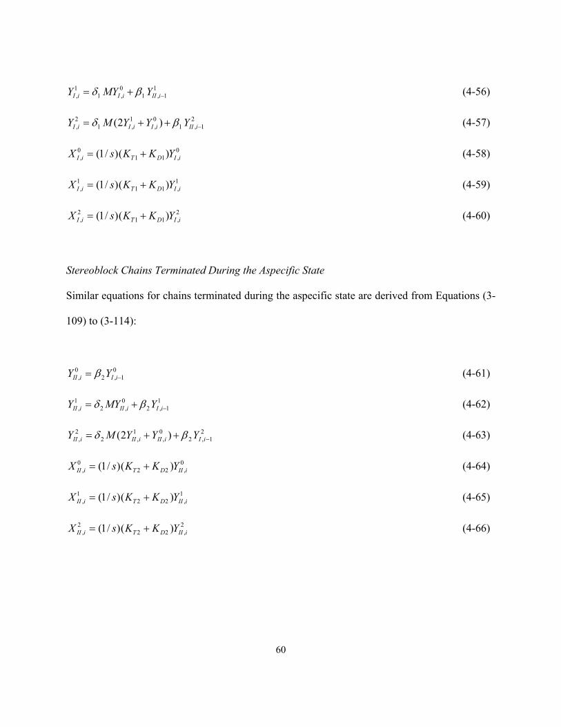
60

11,1

0,1

1, −+= iIIiIiI YMYY βδ ( 4-56)

21,1

0,

1,1

2, )2( −++= iIIiIiIiI YYYMY βδ ( 4-57)

0,11

0, )()/1( iIDTiI YKKsX += ( 4-58)

1,11

1, )()/1( iIDTiI YKKsX += ( 4-59)

2,11

2, )()/1( iIDTiI YKKsX += ( 4-60)

Stereoblock Chains Terminated During the Aspecific State

Similar equations for chains terminated during the aspecific state are derived from Equations (3-

109) to (3-114):

01,2

0, −= iIiII YY β ( 4-61)

11,2

0,2

1, −+= iIiIIiII YMYY βδ ( 4-62)

21,2

0,

1,2

2, )2( −++= iIiIIiIIiII YYYMY βδ ( 4-63)

0,22

0, )()/1( iIIDTiII YKKsX += ( 4-64)

1,22

1, )()/1( iIIDTiII YKKsX += ( 4-65)

2,22

2, )()/1( iIIDTiII YKKsX += ( 4-66)

61

4.2.4 Chain Segments

Isotactic Segments

The equations for the steady-state of the moments of the isotactic segments were solved using

Equations (3-116) to (3-118) and found to be as follows:

MWI''

10 γ= ( 4-67)

01

''1

1II MWMW δγ += ( 4-68)

)2( 011

''1

2III WWMMW ++= δγ ( 4-69)

Atactic Segments

Similarly, the steady-state moments for the atactic segments were derived using Equations (3-

124) to (3-126):

MWII''

21 γ= ( 4-70)

02

''2

1IIII MWMW δγ += ( 4-71)

)2( 012

''2

1IIIIII WWMMW ++= δγ ( 4-72)

62

4.3 Steady-State Simulations

The steady-state equations shown in Section 4.2 were solved simultaneously at different

polymerization conditions. The model was first solved for one single site with two states,

stereospecific (making isotactic chains or blocks) and aspecific (producing atactic chains or

blocks). These simulations represent the main contribution of this thesis, since no mathematical

model for active sites existing in two states has been presented in the literature, even though the

concept has been analyzed qualitatively in many previous publications, as discussed in the

section on literature review.

Ziegler-Natta catalysts, however, have multiple types of sites and only some are considered to go

through this reversible transformation from stereospecific to aspecific state. Most of the other

site types are presumed to make only isotactic polypropylene. Therefore, a four-site model, with

two stereospecific sites and 2 aspecific (two-state) sites, was proposed to model the behaviour of

a heterogeneous Ziegler-Natta catalyst. The number of site types was chosen arbitrarily in our

simulations since we did not make use of experimental data for model validation, but the

predicted trends agree well with the general behaviour of Ziegler-Natta catalysts used

industrially for the production of polypropylene. The following discussion summarizes the

responses to changes in donor type and concentration, catalyst activity and hydrogen

concentration. All of the simulation results presented in this section are tabulated in Appendix A.

63

Figure 4-1 shows that, in the absence of electron donor, no stereoblock chains are made, only

purely atactic or isotactic chains. This is, of course, a consequence of our choice of model

parameters in Table 4-1: the concentration of active sites fed to the reactor in state I and II is the

same and they have the same value for their propagation rate constants; consequently, in the

absence of electron donors, no site transformation will take place and both states will make the

same amount of polymer. Contrarily, when electron donor is introduced in the reactor, a

significant fraction of sites on state II (aspecific) are converted to state I (isospecific), decreasing

the mass fraction of atactic polypropylene to approximately 6%, with the consequent increase in

the fraction of isotactic and stereoblock chains to about 87% and 7%, respectively, as illustrated

in Figure 4-2. Interestingly, according to the simulations, most of the stereoblock chains are

atactic-isotactic diblocks (6 %), with a very low fraction of multiblock chains (1%).

No Donork p 1/k p 2=1

50.00%

0.00%

50.00%

Pure Isotactic Pure Atactic Stereo-Blocks

Block's Distribution

100.00%

0.00%0.00%

0.00%

0.00%0.00%

1 block 2 blocks 3 blocks4 blocks 5 blocks 6 blocks

Figure 4-1: Tacticity and block distributions for propylene made with a single-site catalyst without donor at the reference polymerization conditions. (kp1/kp2 = 1, Rp1/Rtr1 =1364, Rp2/Rtr2 =1364, Mn = 57,270 g/mol, Mw = 114,497 g/mol, and PDI = 2.00)

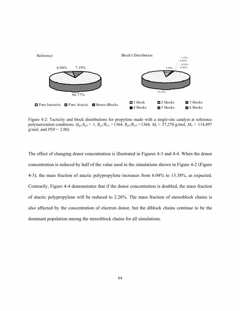
64

Reference

86.77%

7.19%6.04%

Pure Isotactic Pure Atactic Stereo-Blocks

Block's Distribution

92.81%

1.13%0.05%

0.01%0.00%6.00%

1 block 2 blocks 3 blocks4 blocks 5 blocks 6 blocks

Figure 4-2: Tacticity and block distributions for propylene made with a single-site catalyst at reference polymerization conditions. (kp1/kp2 = 1, Rp1/Rtr1 =1364, Rp2/Rtr2 =1364, Mn = 57,270 g/mol, Mw = 114,497 g/mol, and PDI = 2.00)

The effect of changing donor concentration is illustrated in Figures 4-3 and 4-4. When the donor

concentration is reduced by half of the value used in the simulations shown in Figure 4-2 (Figure

4-3), the mass fraction of atactic polypropylene increases from 6.04% to 13.38%, as expected.

Contrarily, Figure 4-4 demonstrates that if the donor concentration is doubled, the mass fraction

of atactic polypropylene will be reduced to 2.26%. The mass fraction of stereoblock chains is

also affected by the concentration of electron donor, but the diblock chains continue to be the

dominant population among the stereoblock chains for all simulations.

65

Block's Distribution

92.98%

6.34% 0.00%0.00%

0.64% 0.03%

1 block 2 blocks 3 blocks4 blocks 5 blocks 6 blocks

1/2 Dok p 1/k p 2=1

79.60%

7.02%13.38%

Pure Isotactic Pure Atactic Stereo-Blocks

Figure 4-3: Tacticity and block distributions for propylene made with a single-site catalyst with half the reference donor concentration shown in Figure 4-2. Other polymerization conditions are the same as shown in Figure 4-1.

2 Dok p 1/k p 2=1

90.91%

6.83%2.26%

Pure Isotactic Pure Atactic Stereo-Blocks

Block's Distribution

93.17%

0.02%

0.07%

0.00%

1.80%

4.93%

1 block 2 blocks 3 blocks4 blocks 5 blocks 6 blocks

Figure 4-4: Tacticity and block distributions for propylene made with a single-site catalyst with twice the reference donor concentration shown in Figure 4-2. Other polymerization conditions are the same as shown in Figure 4-1.

Figure 4-5 shows complete weight distribution for the stereoblock chains and Table 4-7 their

molecular weight averages (Mn, Mw, and PDI). We have also classified the chains according to

the state of the site when chain growth was terminated. This distinction is immaterial for the case

of diblocks, but is important for triblocks and higher odd-numbered multiblock chains, since an

66

isotactic-terminated chain (isotactic-atactic-isotactic-…) has a different microstructure from an

atactic-terminated chain (atactic-isotactic-atactic-…) for odd-numbered multiblock chains. Table

4-7 shows that the molecular weight averages increase and the polydispersity index decreases

with increasing number of blocks per chain. Both trends are expected, since longer chains will

have a higher probability of experiencing site transformation events than shorter chain; the effect

on PDI is a simple consequence of sampling an increasingly narrower polymer population:

uniblock chains are those that follow Flory’s statistics with PDI = 2, diblocks will have PDI =

1.5 in a similar fashion to chains made by termination by combination in free radical

polymerization, and chains with three or more blocks will have even narrower MWDs, since they

are being selected from a subpopulation with increasing molecular weights.

0.00%0.00%

0.00%

0.01%0.08%1.04% 0.03%0.03%

6.04%

3.10%

2.90%

86.77%

1 end Iso 1 end Ata 2 end Iso 2 end Ata3 end Iso 3 end Ata 4 end Iso 4 end Ata5 end Iso 5 end Ata 6 end Iso 6 end Ata

Figure 4-5: Mass fractions of stereoblock chain populations for the reference polymerization conditions shown in Table 4-1.

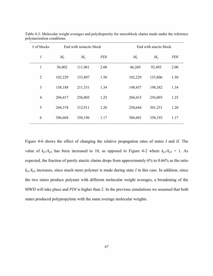
67

Table 4-3: Molecular weight averages and polydispersity for stereoblock chains made under the reference polymerization conditions.

# of blocks End with isotactic block End with atactic block

I Mn Mw PDI Mn Mw PDI

1 56,002 111,961 2.00 46,269 92,495 2.00

2 102,229 153,807 1.50 102,229 153,806 1.50

3 158,188 211,331 1.34 148,457 198,382 1.34

4 204,417 256,005 1.25 204,415 256,003 1.25

5 260,374 312,911 1.20 250,644 301,251 1.20

6 306,604 358,196 1.17 306,601 358,193 1.17

Figure 4-6 shows the effect of changing the relative propagation rates of states I and II. The

value of kp1/kp2 has been increased to 10, as opposed to Figure 4-2 where kp1/kp2 = 1. As

expected, the fraction of purely atactic chains drops from approximately 6% to 0.66% as the ratio

kp1/kp2 increases, since much more polymer is made during state I in this case. In addition, since

the two states produce polymer with different molecular weight averages, a broadening of the

MWD will take place and PDI is higher than 2. In the previous simulations we assumed that both

states produced polypropylene with the same average molecular weights.

68

Normal Dok p 1/k p 2=10

94.56%

0.66% 4.78%

Pure Isotactic Pure Atactic Stereo-Blocks

Block's Distribution

95.22%

0.88% 0.03%0.01%0.00%3.86%

1 block 2 blocks 3 blocks4 blocks 5 blocks 6 blocks

Figure 4-6: Tacticity and block distributions for propylene made with a single-site catalyst at normal donor concentration and increased kp1/kp2 ratio (kp1/kp2 = 10, Rp1/Rtr1 =1364, Rp2/Rtr2 =136, Mn = 52,600 g/mol, Mw = 111,800 g/mol, PDI = 2.13)

The effect of donor type has been also examined by manipulating the values of the parameter for

site transformation by donor, +Dok and −

Dok . Figure 4-7 and Figure 4-8 show the effect of

selecting donor types with different values of site transformation rate constants. When the value

of +Dok is doubled and −

Dok is reduced by a factor of ½ with respect with the value listed in Table

4-2, the mass fraction of purely isotactic chain increases to 95.07 % (as compared to 86.77% for

the reference case) as shown in Figure 4-7; when the value of +Dok is reduced by a factor of ½

and −Dok is doubled, on the other hand, as the mass fraction of purely isotactic chains drops to

65.84 % as presented in Figure 4-8. No significant effect is observed in the values of Mn, Mw,

and PDI, since the propagation and termination rates are not affected by site state transformation.

69

The use of better donors also reduces the weight percent of stereoblock chains, since the

transition from isotactic to atactic state is less likely to occur during the lifetime of a

polypropylene chain.

Donor Bk Do + = 300 L/mol.sk Do - = 0.005 s-1

95.10%

1.25% 3.64%

Pure Isotactic Pure Atactic Stereo-Blocks

Block's Distribution

96.36%

2.68%0.00%

0.01%0.02%0.94%

1 Block 2 Blocks 3 Blocks 4 Blocks5 Blocks 6 Blocks

Figure 4-7: Better donor type effect at steady state reference polymerization conditions for single site. (kDo

+(B)/kDo+(reference) = 2, kDo

−(B)/kDo−(reference) = 0.5, kp1/kp2 = 1, Rp1/Rtr1 =1364, and Rp2/Rtr2 =1364)

70

Donor Ck Do + = 75 L/mol.sk Do - = 0.02 s-1

65.87%

11.74%

22.38%

Pure Isotactic Pure Atactic Stereo-Blocks

Block's Distribution

88.26%

1.21% 0.10%

0.01%0.00%

10.43%

1 Block 2 Blocks 3 Blocks 4 Blocks5 Blocks 6 Blocks

Figure 4-8: Worse donor type effect at steady state reference polymerization conditions for single site, (kDo

+(C)/ kDo+(reference) = 0.5, kDo

− (C)/ kDo−(reference) = 2, kp1/kp2 = 1, Rp1/Rtr1 =1364, and Rp2/Rtr2

=1364)

Figure 4-9 shows how the polymer microstructure is affected when the propagation rate constant

of state I and II are both doubled with respect to the reference case, maintaining the same ratio of

(kp1/kp2), while all other model parameters remain the same. This would correspond to change the

catalyst type or polymerization temperature, for instance although, in reality, all other

polymerization kinetic constants would also be affected by a change of catalyst. As expected, Mn

and Mw almost double when the propagation rate constant is doubled (compare catalyst C2 with

C1). In contrast, catalyst C3 makes polymer with approximately half the Mn and Mw of catalyst

C1, since its propagation rate constant was reduced by a factor of ½. It is interesting to notice

that the tacticities do not change in all three cases, since the value of the propagation rate

constant does not affect the frequency of site state transformation, as shown in Figure 4-9 and

Figure 4-10. This proves that our model equations were properly derived and are consistent with

the expected theoretical behavior for these catalysts.

71

Block's Distribution

92.81%

1.13% 0.05%0.01%0.00%

6.00%

1 Block 2 Blocks 3 Blocks 4 Blocks5 Blocks 6 Blocks

Catalyst C2k pC2 / k pC1 = 2

86.77%

7.19%6.04%

Pure Isotactic Pure Atactic Stereo-Blocks

Figure 4-9: C2 catalyst type at steady state reference polymerization conditions for single site. (kp1/kp2 =

2, Rp1/Rtr1 = Rp2/Rtr2 = 1364, , Mn =114,497 g/mol, and Mw =228,952 g/mol)

Catalyst C3kpC3 / kpC1 = 0.5

86.77%

7.19%6.04%

Pure Isotactic Pure Atactic Stereo-Blocks

Block's Distribution

92.81%

6.00%0.00%0.01%

0.05%1.13%

1 Block 2 Blocks 3 Blocks 4 Blocks5 Blocks 6 Blocks

Figure 4-10: C3 catalyst type at steady state reference polymerization conditions for single site. (kp1/kp2 =

0.5, Rp1/Rtr1 = Rp2/Rtr2 = 1364, , Mn = 28,656 g/mol, and Mw =57,270 g/mol)

Figure 4-11 and Figure 4-12 study the effect of changing the concentration of hydrogen on

polypropylene microstructure. Molecular weight naturally decreases with increasing hydrogen

concentration. More interesting, changes in hydrogen concentration also have a pronounced

72

effect on the fraction of stereoblock chains. This may seem surprising at first, but it is easily

explained: as hydrogen concentration increases, the polymer chains become (in average) shorter

and, consequently, the likelihood of a change in site state taking place during the lifetime of a

polymer chains decreases. Therefore, as the hydrogen concentration increases, the fraction of

stereoblock chains decreases, as illustrated in Figure 4-11.

2 H

88.65%

3.90%7.45%

Pure Isotactic Pure Atactic Stereo-Blocks

Block's Distribution

96.10%

3.56%0.00%0.00%0.01%

0.33%

1 Block 2 Blocks 3 Blocks 4 Blocks5 Blocks 6 Blocks

Figure 4-11: Doubling hydrogen concentration at steady state reference polymerization conditions for

single site. (Mn = 28,689 g/mol, and Mw =57,336 g/mol)

73

1/2 H

83.01%

12.70%4.28%

Pure Isotactic Pure Atactic Stereo-Blocks

Block's Distribution

87.29%

3.33% 0.25%0.08%0.01%

9.04%

1 Block 2 Blocks 3 Blocks 4 Blocks5 Blocks 6 Blocks

Figure 4-12: Decreasing hydrogen concentration by half at steady state reference polymerization conditions for single site. (Mn = 114,214 g/mol, and Mw =228,385 g/mol)

Due to the presence of more than one active site type in heterogenous Ziegler-Natta catalysts

using industrially to polymerize propylene, the model was extended to include multiple sites.

The different active sites on heterogeneous Ziegler-Natta catalysts are characterized by distinct

polymerization kinetic parameters than can be estimated by MWD deconvolution (Faldi and

Soares, 2001; Soares and Hamielec, 1995).

74

Table 4-4: Simulation results for a 4-site model

Site Overall 1 2 3 4

Mole % Mass % Mole % Mass % Mole % Mass % Mole % Mass % Mole % Mass %

Pure Isotactic 95.13% 98.22% 100.0% 100.0% 100.0% 100.0% 91.16% 93.40% 84.84% 86.47%

Pure Atactic 3.41% 0.30% 0.00% 0.00% 0.00% 0.00% 6.41% 2.84% 6.17% 0.88%

Stereoblocks 1.46% 1.48% 0.00% 0.00% 0.00% 0.00% 2.43% 3.76% 8.99% 12.64% Block weight %:

1 block 98.62% 97.98% 100.0% 100.0% 100.0% 100.0% 97.57% 96.24% 91.01% 87.35%

2 blocks 1.12% 1.44% 0.00% 0.00% 0.00% 0.00% 2.22% 3.24% 6.79% 7.89%

3 blocks 0.24% 0.52% 0.00% 0.00% 0.00% 0.00% 0.21% 0.50% 2.00% 4.25%

4 blocks 0.02% 0.04% 0.00% 0.00% 0.00% 0.00% 0.00% 0.01% 0.15% 0.35%

5 blocks 0.00% 0.01% 0.00% 0.00% 0.00% 0.00% 0.00% 0.00% 0.04% 0.14%

6 blocks 0.00% 0.00% 0.00% 0.00% 0.00% 0.00% 0.00% 0.00% 0.00% 0.01%

Mn (g/mol) 52,081 62,957 167,316 7,902 191,523

Mw (g/mol) 231,513 125,890 334,595 16,013 398,055

PDI 4.45 2.00 2.00 2.03 2.08

kp1/kp2 2.50 6.67

Rp1/Rtr1 1500 4000 194 5000

Rp2/Rtr2 0 0 97 1071

Table 4-4 shows the simulation results for a four-site-type catalyst model where model

parameters were chosen so that the overall polymer properties are within values observed in

industrial range. Sites 1 and 2 make only isotactic chains, while Sites 3 and 4 can produce

isotactic, atactic and stereoblock chains because they may exist in two states, as described in our

proposed mechanism above. Site 1 produces isotactic polypropylene chains with Rp1/Rtr1 = 1500

(rate of propagation to rate of termination ratio). However, Site 2 makes chains with longer

average molecular weight with Rp1/Rtr1 = 4000. Sites 3 and 4 can suffer transformation between

75

stereoselective and non stereoselective states by complexation with an electron donor. Site 3 was

assumed to produce around 93 wt% pure isotactic chains, with a ratio of the rate constant of

propagation at stereoselective state to the rate constant of propagation of the non stereoselective

state of kp1/kp2 = 2.5 and shorter chains with Rp1/Rtr1 = 194 and Rp2/Rtr2 = 97. Site 4 was the least

stereoselective site, producing only 86.5 wt % pure isotactic chains with kp1/kp2 = 6.7 and higher

molecular weight averages with Rp1/Rtr1 = 5000 and Rp2/Rtr2 = 1071. Table 4-4 shows that the

model can predict the individual properties of polymer made on each site type such as molecular

weight averages, polydispersity and molar and mass fractions of each population. The overall

properties of the polymer produced by this 4-site catalyst were also predicted where the pure

isotactic content was around 98 wt% and with Mn = 52,081 g/mol, Mw = 231,513 g/mol, and

polydispersity of 4.45. These results are typical of commonly encountered industrial

polypropylene resins made with heterogeneous Ziegler-Natta catalysts.

76

4.4 Dynamic Simulations

In order to compare the steady-state simulations of the previous section and the dynamic

simulations shown in this section, the feed flow rate of catalyst was calculated from Equations

(3-40) and (3-41) assuming steady-state (that is, setting the left hand derivative term to zero) as

follows,

IaI CsAlkC )(ˆ1 += ( 4-73)

IIaII CsAlkC )(ˆ2 += ( 4-74)

Similarly, the feed flow rates of all other reagents were calculated from their dynamic mass

balances given below

))()(

(ˆd

d

220

110

22201110

skkYkkY

kPkPkPkPkPkPMMt

M

MpIIMpI

iRII

EtiHII

HiII

iRI

EtiHI

HiI

+++++

+++++−= ( 4-75)

)(ˆd

d 02

01 sYkYkHH

tH

IIHIH ++−= ( 4-76)

)(ˆd

ld 02

0121 sYkYkIkCkCkAllA

tA

IIAlIAlAlIIaIa +++++−= ( 4-77)

))(()(ˆd

d 00

00 sYPPPkDoYPPPkoD

tDo

IIII

EtII

HII

DoII

EtI

HI

Do ++++−++++= +− ( 4-78)

77

By solving these equations at steady –state (as indicated below), we are able to obtain the molar

flow rates for each of the reactants,

))()(

(ˆ

220

110

22201110

skkYkkY

kPkPkPkPkPkPMM

MpIIMpI

iRII

EtiHII

HiII

iRI

EtiHI

HiI

++++−

+++++= ( 4-79)

)(ˆ 02

01 sYkYkHH IIHIH ++= ( 4-80)

)(ˆ 02

0121 sYkYkIkCkCkAllA IIAlIAlIAlIIaIa +++++= ⋅ ( 4-81)

)())((ˆ 00

00 I

IEt

IH

IDoII

IIEt

IIH

IIDo YPPPksYPPPkDooD +++−++++= −+ ( 4-82)

Since some feed rates depend on more than one reference concentration, different feed flow rates

will result when concentrations are changed. For instance, the propylene flow rate calculated for

the reference conditions CI = CII = 0.00001, M = 0.2, Al = Do = 0.0007, and H = 0.004 mol/L, is

19.633 mol/s. However, when the hydrogen concentration is double to H = 0.008 mol/L, the

propylene flow rate changes to 15.9 mol/s as shown in Table 4-5.

The dynamic population balances derived in Section 3.3.4 to 3.3.6 were solved using the

“ode15s” solver in MATLAB (Higham and Higham, 2005). The effect of changing the

concentrations of donor, hydrogen, and propylene on polymer microstructure was studied by

manipulating their feed rates as shown in Table 4-5. The input data used in the dynamic

simulations is identical to those used for the steady-state simulations. All initial values of

concentrations and moments were set to zero; therefore, the simulations reflect a reactor start-up

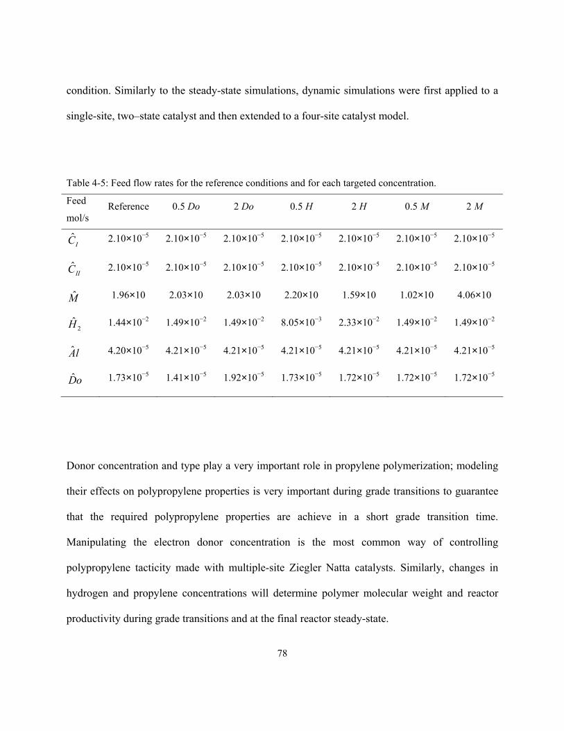
78

condition. Similarly to the steady-state simulations, dynamic simulations were first applied to a

single-site, two–state catalyst and then extended to a four-site catalyst model.

Table 4-5: Feed flow rates for the reference conditions and for each targeted concentration.

Feed

mol/s Reference 0.5 Do 2 Do 0.5 H 2 H 0.5 M 2 M

IC 2.10×10−5 2.10×10−5 2.10×10−5 2.10×10−5 2.10×10−5 2.10×10−5 2.10×10−5

IIC 2.10×10−5 2.10×10−5 2.10×10−5 2.10×10−5 2.10×10−5 2.10×10−5 2.10×10−5

M 1.96×10 2.03×10 2.03×10 2.20×10 1.59×10 1.02×10 4.06×10

2H 1.44×10−2 1.49×10−2 1.49×10−2 8.05×10−3 2.33×10−2 1.49×10−2 1.49×10−2

lA 4.20×10−5 4.21×10−5 4.21×10−5 4.21×10−5 4.21×10−5 4.21×10−5 4.21×10−5

oD 1.73×10−5 1.41×10−5 1.92×10−5 1.73×10−5 1.72×10−5 1.72×10−5 1.72×10−5

Donor concentration and type play a very important role in propylene polymerization; modeling

their effects on polypropylene properties is very important during grade transitions to guarantee

that the required polypropylene properties are achieve in a short grade transition time.

Manipulating the electron donor concentration is the most common way of controlling

polypropylene tacticity made with multiple-site Ziegler Natta catalysts. Similarly, changes in

hydrogen and propylene concentrations will determine polymer molecular weight and reactor

productivity during grade transitions and at the final reactor steady-state.

79

Figure 4-13 shows that doubling the donor concentration does not affect the value of the

molecular weight averages of the polymer. On the other hand, Mn and Mw decrease when the

hydrogen concentration is doubled and increase when the propylene concentration is doubled, as

expected from the polymerization model adopted for these simulations. The dynamic simulations

shown in Figure 4-13 capture nicely the overall reactor dynamics and the time elapsed between

the grade transitions.

Figure 4-14 shows how changing the same concentrations affects the stereoregularity of the

polymer. The mass fraction of isotactic chains increases from approximately 86.8 % to 90.9 %

by doubling the donor concentration, while the mass fraction of atactic chains drops from 6.0 %

to 2.3 % and stereoblock chains from 7.2 % to approximately 6.8 %. It is also interesting to see

that, by doubling the concentration of hydrogen, the mass fraction of isotactic chains drops to

88.7 % which is still higher than the reference value 86.8 % and the mass fraction of the atactic

chains increases by 1.5 % from its reference value of 6.0 %. However, the mass fraction of the

stereoblock chains drops from 7.2 % to approximately 3.9 %. Moreover, by doubling the

concentration of monomer, the fractions of isotactic, atactic, and stereoblock chains are not

affected, because monomer concentration affects propagation rate only and does not have any

effect on site transformation rate.

80

1 2 3 4 5 6 7

x 10 4

0.5

1

1.5

2

2.5

3

3.5

4

x 10 5M

olec

ular

Wei

ght (

g/m

ol)

Time ( s )

Normal Conditions 2 [Do] 2 [H2] 2 [M]

86.7 % Isotactic

90.9 % Isotactic

88.6 % Isotactic

86.7 % Isotactic

Mw

Mn

1 2 3 4 5 6 7

x 10 4

0.5

1

1.5

2

2.5

3

3.5

4

x 10 5M

olec

ular

Wei

ght (

g/m

ol)

Time ( s )

Normal Conditions 2 [Do] 2 [H2] 2 [M]

86.7 % Isotactic

90.9 % Isotactic

88.6 % Isotactic

86.7 % Isotactic

1 2 3 4 5 6 7

x 10 4

0.5

1

1.5

2

2.5

3

3.5

4

x 10 5M

olec

ular

Wei

ght (

g/m

ol)

Time ( s )1 2 3 4 5 6 7

x 10 4

0.5

1

1.5

2

2.5

3

3.5

4

x 10 5M

olec

ular

Wei

ght (

g/m

ol)

Time ( s )

Normal Conditions 2 [Do] 2 [H2] 2 [M]

86.7 % Isotactic

90.9 % Isotactic

88.6 % Isotactic

86.7 % Isotactic

Normal Conditions 2 [Do] 2 [H2] 2 [M]Normal Conditions

Normal Conditions 2 [Do]2 [Do] 2 [H2]2 [H2] 2 [M]2 [M]

86.7 % Isotactic

90.9 % Isotactic

88.6 % Isotactic

86.7 % Isotactic

86.7 % Isotactic

90.9 % Isotactic

88.6 % Isotactic

86.7 % Isotactic

Mw

Mn

Figure 4-13: Effect of changing the concentrations of donor, hydrogen, and monomer on Mn and Mw.

81

0 1 2 3 4 5 6 7 8

x 10 4

0

10

20

30

40

50

60

70

80

90

100

Mas

s %

Time ( s )

Isotactic

Atactic

Stereoblocks

Stereoblocks

Atactic

Isotactic

Normal Conditions 2 [Do] 2 [H2] 2 [M]

Mn = 57,000Mw = 114,000

Mn = 57,000Mw = 114,000

Mn = 28,500Mw = 57,000

Mn = 115,000Mw = 231,000

0 1 2 3 4 5 6 7 8

x 10 4

0

10

20

30

40

50

60

70

80

90

100

Mas

s %

Time ( s )

Isotactic

Atactic

Stereoblocks

Stereoblocks

Atactic

Isotactic

0 1 2 3 4 5 6 7 8

x 10 4

0

10

20

30

40

50

60

70

80

90

100

Mas

s %

Time ( s )

0 1 2 3 4 5 6 7 8

x 10 4

0

10

20

30

40

50

60

70

80

90

100

Mas

s %

Time ( s )

Isotactic

Atactic

Stereoblocks

Stereoblocks

Atactic

Isotactic

Normal Conditions 2 [Do] 2 [H2] 2 [M]

Mn = 57,000Mw = 114,000

Mn = 57,000Mw = 114,000

Mn = 28,500Mw = 57,000

Mn = 115,000Mw = 231,000

Normal Conditions

Normal Conditions 2 [Do]2 [Do] 2 [H2]2 [H2] 2 [M]2 [M]

Mn = 57,000Mw = 114,000

Mn = 57,000Mw = 114,000

Mn = 28,500Mw = 57,000

Mn = 115,000Mw = 231,000

Figure 4-14: Effect of changing the concentration of donor, hydrogen, and monomer on mass fraction of isotactic, atactic and stereoblock chains.

As demonstrated with the steady-state model, the molecular weights obtained for the stereoblock

chains increase with the number of blocks in the chain, while their polydispersities decrease. The

same phenomenon is predicted with the dynamic model, as illustrated in Figure 4-15 and Figure

4-16.

Variation in the properties of stereoblock chains was also studied as a function of donor,

hydrogen, and monomer concentrations. Figure 4-17 shows that the number average molecular

82

weight of chains with one to four stereoblocks increases very slightly when the concentration of

electron donor is reduced. This is easy to understand, since the donor acts as a “pseudo chain

transfer agent”, shortening the average lengths of a stereoblock as it transforms the site from the

aspecific to the stereospecific state, and vice-versa as shown in Figure 4-18. Similarly, a decrease

in the concentration of the actual chain transfer agent, hydrogen, will lead to an increase in the

molecular weight averages of the stereoblocks, in this case much more pronounced. Differently,

a decrease in monomer concentration will lead to a drop in the average size of the stereoblocks.

0 500 1000 1500 2000 2500 30000

0.5

1

1.5

2

2.5

3

3.5x 10 5 Blocks @ Normal Condition : Molecular Weights vs. Time

Mol

ecul

ar W

eigh

t (g/

mol

)

Time "Sec"

Mn Block 1Mn Block 2Mn Block 3Mn Block 4Mn Block 5Mn Block 6Mw Block 1Mw Block 2Mw Block 3Mw Block 4Mw Block 5Mw Block 6

0 500 1000 1500 2000 2500 30000

0.5

1

1.5

2

2.5

3

3.5x 10 5 Blocks @ Normal Condition : Molecular Weights vs. Time

Mol

ecul

ar W

eigh

t (g/

mol

)

Time "Sec"

Mn Block 1Mn Block 2Mn Block 3Mn Block 4Mn Block 5Mn Block 6Mw Block 1Mw Block 2Mw Block 3Mw Block 4Mw Block 5Mw Block 6

( s )0 500 1000 1500 2000 2500 3000

0

0.5

1

1.5

2

2.5

3

3.5x 10 5 Blocks @ Normal Condition : Molecular Weights vs. Time

Mol

ecul

ar W

eigh

t (g/

mol

)

Time "Sec"

Mn Block 1Mn Block 2Mn Block 3Mn Block 4Mn Block 5Mn Block 6Mw Block 1Mw Block 2Mw Block 3Mw Block 4Mw Block 5Mw Block 6

0 500 1000 1500 2000 2500 30000

0.5

1

1.5

2

2.5

3

3.5x 10 5 Blocks @ Normal Condition : Molecular Weights vs. Time

Mol

ecul

ar W

eigh

t (g/

mol

)

Time "Sec"

Mn Block 1Mn Block 2Mn Block 3Mn Block 4Mn Block 5Mn Block 6Mw Block 1Mw Block 2Mw Block 3Mw Block 4Mw Block 5Mw Block 6

0 500 1000 1500 2000 2500 30000

0.5

1

1.5

2

2.5

3

3.5x 10 5 Blocks @ Normal Condition : Molecular Weights vs. Time

Mol

ecul

ar W

eigh

t (g/

mol

)

Time "Sec"

Mn Block 1Mn Block 2Mn Block 3Mn Block 4Mn Block 5Mn Block 6Mw Block 1Mw Block 2Mw Block 3Mw Block 4Mw Block 5Mw Block 6

0 500 1000 1500 2000 2500 30000

0.5

1

1.5

2

2.5

3

3.5x 10 5 Blocks @ Normal Condition : Molecular Weights vs. Time

Mol

ecul

ar W

eigh

t (g/

mol

)

Time "Sec"

Mn Block 1Mn Block 2Mn Block 3Mn Block 4Mn Block 5Mn Block 6Mw Block 1Mw Block 2Mw Block 3Mw Block 4Mw Block 5Mw Block 6

( s )

Figure 4-15: Dynamic evolution of molecular weight averages for chains with different number of stereoblocks. (One block accounts for both isotactic and atactic chains).

83

1000 2000 3000 4000 5000 6000 7000

1

1.2

1.4

1.6

1.8

2

2.2

2.4

2.6

2.8

PDI

Time "Sec"

PDI Block 1PDI Block 2

PDI Block 3

PDI Block 4

PDI Block 5PDI Block 6

1000 2000 3000 4000 5000 6000 7000

1

1.2

1.4

1.6

1.8

2

2.2

2.4

2.6

2.8

PDI

Time "Sec"

PDI Block 1PDI Block 2

PDI Block 3

PDI Block 4

PDI Block 5PDI Block 6

Figure 4-16: Dynamic evolution of polydispersity for chains with different numbers of stereoblocks.

84

1 2 3 4 5 6 7 8

x 10 4

0

1

2

3

4

5

x 10 5

Mol

ecul

ar W

eigh

t (g/

mol

)

Time ( s )

Reference Conditions 1/2 Do 1/2 M

86.7 % Isotactic

67.5 % Isotactic

82.8 % Isotactic

86.7 % Isotactic

1/2 H2

Chains with one block

Chains with 2 blocks

Chains with 3 blocks

Chains with 4 blocks

1 2 3 4 5 6 7 8

x 10 4

0

1

2

3

4

5

x 10 5

Mol

ecul

ar W

eigh

t (g/

mol

)

Time ( s )

Reference Conditions 1/2 Do 1/2 M

86.7 % Isotactic

67.5 % Isotactic

82.8 % Isotactic

86.7 % Isotactic

1/2 H2

1 2 3 4 5 6 7 8

x 10 4

0

1

2

3

4

5

x 10 5

Mol

ecul

ar W

eigh

t (g/

mol

)

Time ( s ) 1 2 3 4 5 6 7 8

x 10 4

0

1

2

3

4

5

x 10 5

Mol

ecul

ar W

eigh

t (g/

mol

)

Time ( s )

Reference Conditions 1/2 Do 1/2 M

86.7 % Isotactic

67.5 % Isotactic

82.8 % Isotactic

86.7 % Isotactic

1/2 H2

Reference ConditionsReference Conditions 1/2 Do1/2 Do 1/2 M1/2 M

86.7 % Isotactic

67.5 % Isotactic

82.8 % Isotactic

86.7 % Isotactic

1/2 H21/2 H2

Chains with one block

Chains with 2 blocks

Chains with 3 blocks

Chains with 4 blocks

Chains with one block

Chains with 2 blocks

Chains with 3 blocks

Chains with 4 blocks

Figure 4-17: Number average molecular weights (Mn) responses to the reduction of donor, hydrogen, and monomer concentrations for chains with one to four blocks (One block accounts for both isotactic and atactic chains).

85

1 2 3 4 5 6 7 8

x 10 4

0

1

2

3

4

5

6

x 10 5

Mol

ecul

ar W

eigh

t (g/

mol

)

Time ( s )

ReferenceConditions 2 Do

86.7 % Isotactic

90.9 % Isotactic

88.6 % Isotactic

86.7 % Isotactic

2 H2

2 M

Chains with one block

Chains with 2 blocks

Chains with 3 blocks

Chains with 4 blocks

1 2 3 4 5 6 7 8

x 10 4

0

1

2

3

4

5

6

x 10 5

Mol

ecul

ar W

eigh

t (g/

mol

)

Time ( s )

ReferenceConditions 2 Do

86.7 % Isotactic

90.9 % Isotactic

88.6 % Isotactic

86.7 % Isotactic

2 H2

2 M

1 2 3 4 5 6 7 8

x 10 4

0

1

2

3

4

5

6

x 10 5

Mol

ecul

ar W

eigh

t (g/

mol

)

Time ( s ) 1 2 3 4 5 6 7 8

x 10 4

0

1

2

3

4

5

6

x 10 5

Mol

ecul

ar W

eigh

t (g/

mol

)

Time ( s )

ReferenceConditions 2 Do

86.7 % Isotactic

90.9 % Isotactic

88.6 % Isotactic

86.7 % Isotactic

2 H2

2 M

ReferenceConditionsReferenceConditions 2 Do2 Do

86.7 % Isotactic

90.9 % Isotactic

88.6 % Isotactic

86.7 % Isotactic

2 H22 H2

2 M2 M

Chains with one block

Chains with 2 blocks

Chains with 3 blocks

Chains with 4 blocks

Chains with one block

Chains with 2 blocks

Chains with 3 blocks

Chains with 4 blocks

Figure 4-18: Number average molecular weights (Mn) responses to the increase of donor, hydrogen, and monomer concentrations for chains containing from one to four blocks.

4.5 Comparison between Steady-State and Dynamic Solutions

To insure the accuracy of both dynamic and steady-state simulations, we compared the steady-

state results of the dynamic simulation with those obtained with the steady-state model. Tables 4-

6 to 4-8 show that both simulation methods are in excellent agreement for all predicted

properties. The slight differences shown in those tables are due to round off errors between the

different mathematical techniques used to solve the steady-state and dynamic problems.

86

Table 4-6: Comparison of one-site steady-state and dynamic models: Overall properties.

Mass % Steady State Dynamic Difference %

Pure Isotactic 86.73% 86.68% -0.1%

Pure Atactic 6.07% 6.10% 0.5%

Stereo-Blocks 7.20% 7.22% 0.2%

By Block

1 block 92.81% 92.81% 0.0 %

2 blocks 6.00% 6.00% 0.0 %

3 blocks 1.13% 1.13% 0.0 %

4 blocks 0.05% 0.05% 0.0 %

5 blocks 0.01% 0.01% 0.0 %

6 blocks 0.00% 0.00% 0.0 %

Mn (g/mol) 57,270 57,270 0.0 %

Mw (g/mol) 114,497 114,497 0.0 %

PDI 2.00 2.00 0.0 %

87

Table 4-7: Comparison of one-site steady-state and dynamic models: Stereoblock properties.

Steady State Dynamic Difference %

i Mn Mw PDI Mn Mw PDI Mn Mw PDI

1 55,246 110,695 2.00 55,245 110,690 2.00 0.00% 0.00% 0.00%

2 102,229 153,807 1.50 102,230 153,810 1.50 0.00% 0.00% 0.00%

3 157,432 210,382 1.34 157,430 210,380 1.34 0.00% 0.00% 0.00%

4 204,416 256,004 1.25 204,420 256,010 1.25 0.00% 0.00% 0.00%

5 259,619 312,037 1.20 259,620 312,040 1.20 0.00% 0.00% 0.00%

6 306,603 358,194 1.17 306,610 358,200 1.17 0.00% 0.00% 0.00%

Table 4-8: Comparison of one-site steady-state and dynamic models: Chain segment properties

Steady State Dynamic Difference %

Mn Mw PDI Mn Mw PDI Mn Mw PDI

Isotactic

segments 56,008 111,939 2.00

56,002 111,960 2.00

0.01% -0.02% -0.03%

Atactic

segments 46,274 92,507 2.00

46,271 92,500 2.00

0.01% 0.01% 0.00%

All

segments 55,058 110,377 2.00

55,112 110,470 2.00

-0.01% -0.08% 0.01%

88

Chapter 5

Monte Carlo Simulation

5.1 Mechanistic Approach

Monte Carlo simulation uses randomly generated numbers to select one event from a series of

events based on its probability of occurrence. For our model of olefin polymerization,

probabilities can be defined for propagation, termination, and transformation. Since the chains

are made one-by-one, the maximum microstructural information can be obtained by Monte Carlo

simulation. In olefin polymerization, several researchers have used Monte Carlo simulation to

keep track of microstructural information that could not be achieved by other modeling

techniques. Soares (2006) summarized Monte Carlo simulation techniques for single-site

catalysts and illustrated some of its applications. Simon and Soares (2002) used a Monte Carlo

model to describe the long-chain branch formation in polyethylene made with a combination of

single-site catalysts. A Monte Carlo model was also used to analyze the microstructure of

polyolefin thermoplastic elastomers made with two single-site catalysts (Haag et al., 2003).

Furthermore, Beigzadeh et al. (2001) simulated CRYSTAF fractionation of ethylene/1-octene

copolymers made with single-site catalysts using a Monte Carlo model.

In this chapter, we used Monte Carlo techniques to develop a new model to simulate propylene

polymerization taking in consideration site transformation in the presence of electron donors.

89

The model can predict the same properties modeled by the method of moments and, in addition,

the complete MWD of the several polymer populations.

Figure 5-1 shows the algorithm developed for the one-site, two–state catalyst model. The model

consists of two main loops: one for constructing the isotactic segments (growing when the site is

in the isospecific state) and the other for constructing the atactic segments (when the site is in the

aspecific state). In each loop, propagation, termination or state transformation events may take

place. The probabilities for each event have been calculated using the values of the kinetic

constants and polymerization conditions, as will be explained in Figure 5-1. The algorithm starts

by generating a random number (Rand), uniformly distributed between zero and one, which is

then used to select a reaction step. The algorithm generally starts with the site in the most

probable state, the isospecific state I, but the choice of initial state will not affect the outcome of

the simulations. This algorithm was coded using MATLAB. It takes apperoximatly 80 minutes to

simulate the full molecular weight distribution for about 205,000 chains and approximately 230

minutes for the NMR prediction with around 900,000 sequences using an AMD Turion 64x2, 1.6

GHz, and 512KB L2 cache.

90

Figure 5-1: Monte Carlo simulation flowchart.

Another chain ?

Another chain ?

r = 0

Rand

Save chain information

End

Start

Yes Rand < Pp2

Pp1 , Ptr1, Ptf1 Pp2 , Ptr2, Ptf2

Yes

State = 1 ?

Yes

Rand < Pp1?

r = r + 1 r = r + 1

No

Rand < Pp2+Ptr2

Rand < Pp1+Ptr1

Yes

No No

Yes No

State = 1 State = 2

Save chain information

No Yes

No No

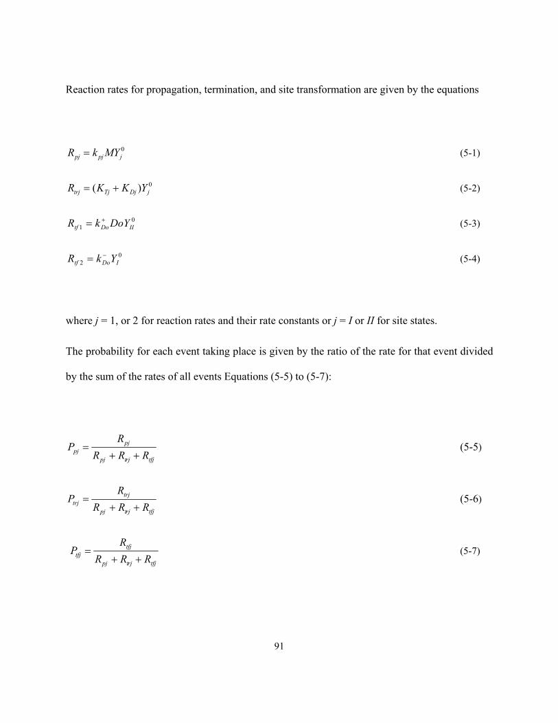
91

Reaction rates for propagation, termination, and site transformation are given by the equations

0jpjpj MYkR = ( 5-1)

0)( jDjTjtrj YKKR += ( 5-2)

01 IIDotf DoYkR += ( 5-3)

02 IDotf YkR −= ( 5-4)

where j = 1, or 2 for reaction rates and their rate constants or j = I or II for site states.

The probability for each event taking place is given by the ratio of the rate for that event divided

by the sum of the rates of all events Equations (5-5) to (5-7):

tfjrjtpj

pjpj RRR

RP

++= ( 5-5)

tfjrjtpj

trjtrj RRR

RP

++= ( 5-6)

tfjrjtpj

tfjtfj RRR

RP

++= ( 5-7)

92

where Ppj is the probability of propagation, Ptrj is the probability of termination, and Ptfj is the

probability of transformation at state j = 1 or 2.

5.2 Simulation Results

Figure 5-2 shows the full chain length distributions (CLDs) for all polymer chains, isotactic,

atactic, and stereoblock chains predicted for the polymerization at the reference conditions

shown in Table 4-1 and Table 4-2. The random noise observed in the CLD is characteristic of

Monte Carlo simulations and can be reduced by generating more polymer chains. For the present

simulation, over 205,000 polymer chains were generated. This type of detailed microstructural

information can only be obtained by the complete solution of the population balances or by

Monte Carlo simulation. Monte Carlo simulation is usually much easier to implement, albeit it

may require considerable computational time. In the case of the reference electron donor

concentration, the mass fraction of isotactic chains was approximately 87.2 %, of atactic 5.6 %,

and of stereoblock 7.2 % (the area under the CLDs is proportional to the mass fraction of

polymer belonging to that population). The model can also predict number and weight average

molecular weights for the overall polymer (Mn= 57,212 Mw= 114,600, and PDI = 2.0.), isotactic

(Mn = 56,819 , Mw = 113,620, PDI = 2.0), atactic (Mn = 45,612 , Mw = 89,699, PDI = 2.0), and

stereoblock chains (Mn = 113,780 , Mw = 169,830 and PDI = 1.5). Figure 5-3, shows that the

Monte Carlo and method of moments predictions for molecular weights and polydispersities

agree very well with increasing number of Monte Carlo iterations (an iteration counts the number

93

of propagation, termination or site transformation events during the simulation) Similarly, Figure

5-4 demonstrates that tacticity predictions by both models are in good agreement, proving that

both models describe the polymerization adequately.

0 0.2 0.4 0.6 0.8 1 1.2 1.4 1.6 1.8 2

x 104

0

0.01

0.02

0.03

0.04

0.05

0.06

Chain Length

Wei

ght F

ract

ion

OverallPure IsotacticPure AtacticSetreoblocks

0 0.2 0.4 0.6 0.8 1 1.2 1.4 1.6 1.8 2

x 104

0

0.01

0.02

0.03

0.04

0.05

0.06

Chain Length

Wei

ght F

ract

ion

OverallPure IsotacticPure AtacticSetreoblocks

Figure 5-2: Monte Carlo simulation of the chain length distributions at reference polymerization conditions; Mn= 57,212 Mw= 114,600, PDI = 2.0, Isotactic = 87.2%, Atactic = 5.6%, Stereoblocks = 7.2%, and with total number of chains of 205,750.

94

113,000

113,500

114,000

114,500

115,000

0.E+00 5.E+07 1.E+08 2.E+08 2.E+08 3.E+08 3.E+08

Iteration

Mw

(g/m

ol)

56,800

56,900

57,000

57,100

57,200

57,300

57,400

57,500

57,600

Mn

(g/m

ol)

Mw

MM_Mw

Mn

MM_Mn

Figure 5-3: Molecular weight averages at reference polymerization conditions: Monte Carlo versus method of moments (MM).

95

85.4

85.9

86.4

86.9

87.4

87.9

88.4

1.0E+07 6.0E+07 1.1E+08 1.6E+08 2.1E+08 2.6E+08 3.1E+08 3.6E+08

Iteration

Isot

actic

Wei

ght %

4.5

5

5.5

6

6.5

7

7.5

8

8.5

Ata

ctic

Wei

ght %

Iso %

MM_Iso%

Ata %

MM_Ata%

Stereo %

MM_Stereo%

Figure 5-4: Tacticity distribution at reference polymerization conditions: Monte Carlo versus method of moments (MM); for reference polymerization conditions, refer to Table 4-1 and 4-2.

96

0 0.2 0.4 0.6 0.8 1 1.2 1.4 1.6 1.8 2

x 104

0

0.01

0.02

0.03

0.04

0.05

0.06

Chain Length

Wei

ght F

ract

ion

OverallPure IsotacticPure AtacticSetreoblocks

0 0.2 0.4 0.6 0.8 1 1.2 1.4 1.6 1.8 2

x 104

0

0.01

0.02

0.03

0.04

0.05

0.06

Chain Length

Wei

ght F

ract

ion

OverallPure IsotacticPure AtacticSetreoblocks

Figure 5-5: Monte Carlo simulation of the chain length distribution at 2×Do; Mn= ,57,106 Mw= 114,460, PDI = 2.0, Isotactic = 91.1%, Atactic = 2.1%, Stereoblocks = 6.8%, and with total number of chains of 205,780.

Similar CLDs are shown in Figure 5-5 for the case when the concentration of electron donor is

doubled. In this case, the mass fraction of isotactic chains increased to 91.1 %, that of atactic

chains decreased to 2.1 %, and the mass fraction of stereoblock chains change only slightly to

6.8 %. The predicted number and weight average molecular weights for the overall polymer (Mn

= 57,106, Mw = 114,460, PDI = 2.0), isotactic (Mn = 55,810, Mw = 111,840, PDI = 2.0), atactic

(Mn = 37,942, Mw = 75,625, PDI = 2.0), and stereoblock chains (Mn = 106, 640, Mw = 161,420,

97

PDI = 1.51) are also predicted easily by the Monte Carlo simulation. These results are also in

excellent agreement in terms of their molecular weights with those obtained through the method

of moments model shown previously in Figure 4-4.

0 0.2 0.4 0.6 0.8 1 1.2 1.4 1.6 1.8 2

x 104

0

0.01

0.02

0.03

0.04

0.05

0.06

Chain Length

Wei

ght F

ract

ion

OverallPure IsotacticPure AtacticSetreoblocks

0 0.2 0.4 0.6 0.8 1 1.2 1.4 1.6 1.8 2

x 104

0

0.01

0.02

0.03

0.04

0.05

0.06

Chain Length

Wei

ght F

ract

ion

OverallPure IsotacticPure AtacticSetreoblocks

Figure 5-6: Monte Carlo simulation of the chain length distributions at ½ × Do ; Mn= 57,098 Mw = 114,530, PDI = 2.0, Isotactic = 80.1%, Atactic = 12.9%, Stereoblocks = 7.1%, and with total number of chains of 205,800.

On the other hand, Figure 5-6 shows the CLDs predicted when the donor concentration is

reduced to half its reference value: the mass fraction of isotactic chains decrease to 80.1 %, while

98

that of atactic chains increase to 12.9 % and stereoblock chains have a slight decrease to 7.1 %.

The predicted number and weight average molecular weights were for the overall polymer (Mn =

57,098 , Mw = 114,530, PDI = 2.0), isotactic (Mn = 55,824, Mw = 111,940, PDI = 2.0), atactic

(Mn = 51,185, Mw = 102,248, PDI = 2.0), and stereoblock chains (Mn = 110,660, Mw = 165,860,

PDI = 1.5) are predicted and agree with the results from the method of moments shown Figure

4-3.

5.3 13C NMR Simulation

One of the most common techniques for determining the degree of tacticity in polypropylene is

carbon-13 nuclear magnetic resonance (13C NMR). 13C NMR measures the sequence distribution

of meso (isotactic, m) and racemic (syndiotactic, r) placements of the methyl groups along the

polymer chain. Figure 5-7 shows the two possible dyad arrangements. Triad, tetrad, pentad and

higher sequences are similarly defined, as illustrated for a particular sequence in Figure 5-8.

Figure 5-7: Dyad arrangements (m = meso, r = racemic).

m r

99

Figure 5-8: Higher meso and racemic sequence distributions.

These sequences obey the following mathematical relationships that will be used later for

verification of our Monte Carlo model (Odian, 2004):

1=+ rm ( 5-8)

1=++ mrrrmm ( 5-9)

mrmmm 5.0+= ( 5-10)

mrrrr 5.0+= ( 5-11)

mmrmmmmm 5.0+= ( 5-12)

mrmmrrrmrmmrmr 22 +=+= ( 5-13)

mmrrmmrmrmmrmmmr +=+ 2 ( 5-14)

rrmmrrmrmrrmmrr +=+ 2 ( 5-15)

mmmrmmmmmmm 5.0+= ( 5-16)

mmrrmmrmrmmrmmmrmmr +=+= 2 ( 5-17)

rmrrmrmrrmr 5.05.0 += ( 5-18)

m r r rm m

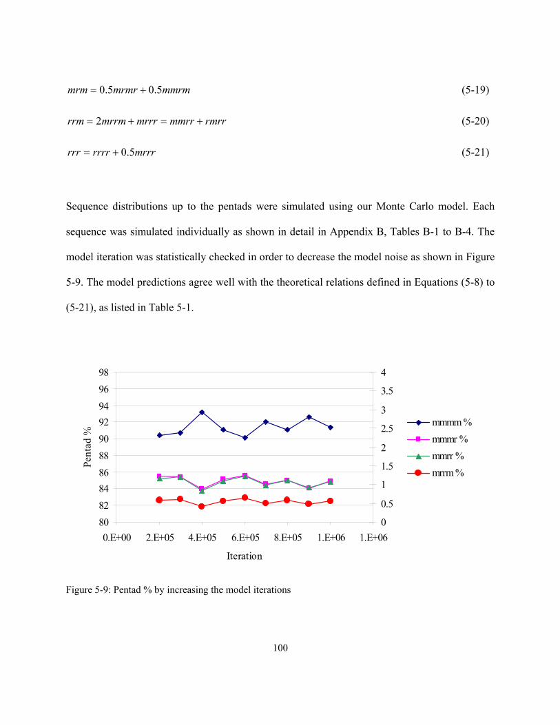
100

mmrmmrmrmrm 5.05.0 += ( 5-19)

rmrrmmrrmrrrmrrmrrm +=+= 2 ( 5-20)

mrrrrrrrrrr 5.0+= ( 5-21)

Sequence distributions up to the pentads were simulated using our Monte Carlo model. Each

sequence was simulated individually as shown in detail in Appendix B, Tables B-1 to B-4. The

model iteration was statistically checked in order to decrease the model noise as shown in Figure

5-9. The model predictions agree well with the theoretical relations defined in Equations (5-8) to

(5-21), as listed in Table 5-1.

80828486889092949698

0.E+00 2.E+05 4.E+05 6.E+05 8.E+05 1.E+06 1.E+06

Iteration

Pent

ad %

0

0.5

1

1.5

2

2.5

3

3.5

4

mmmm %mmmr %mmrr %mrrm %

Figure 5-9: Pentad % by increasing the model iterations

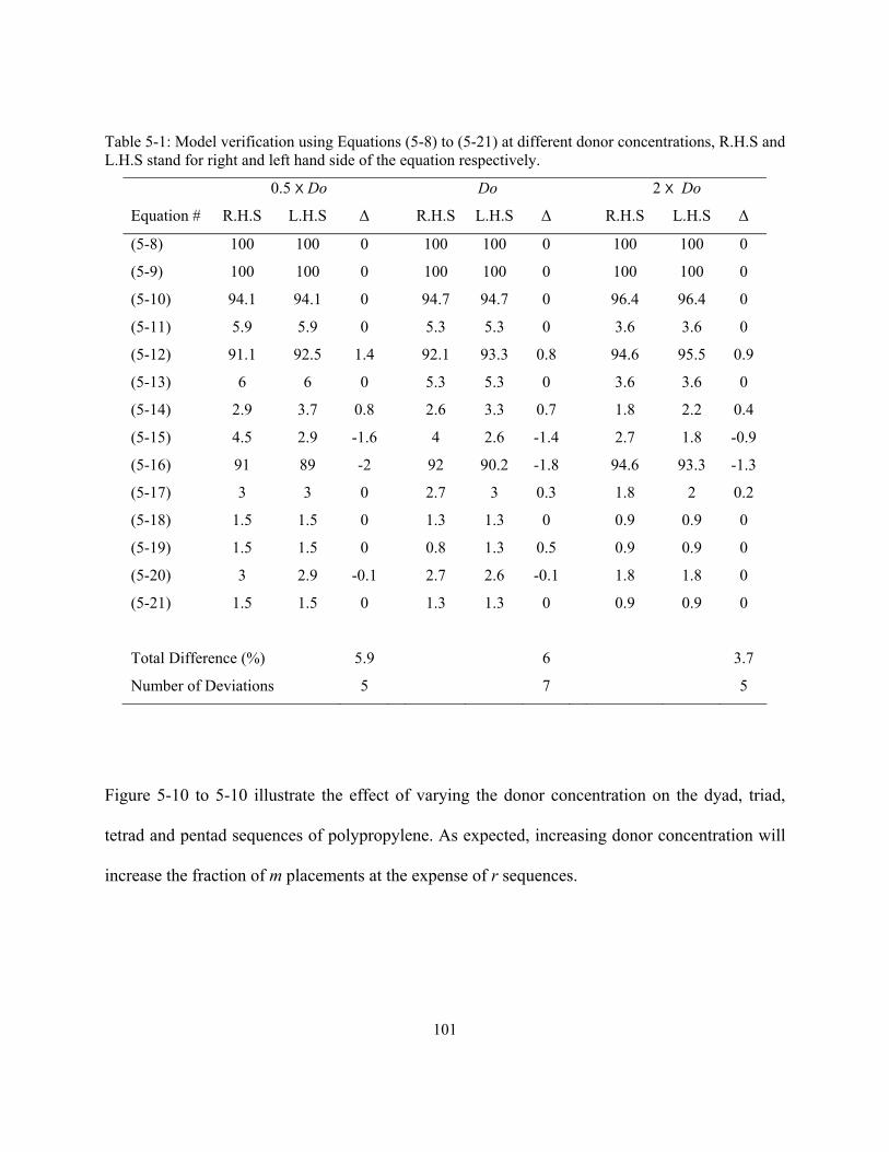
101

Table 5-1: Model verification using Equations (5-8) to (5-21) at different donor concentrations, R.H.S and L.H.S stand for right and left hand side of the equation respectively.

0.5 X Do Do 2 X Do

Equation # R.H.S L.H.S Δ R.H.S L.H.S Δ R.H.S L.H.S Δ

(5-8) 100 100 0 100 100 0 100 100 0

(5-9) 100 100 0 100 100 0 100 100 0

(5-10) 94.1 94.1 0 94.7 94.7 0 96.4 96.4 0

(5-11) 5.9 5.9 0 5.3 5.3 0 3.6 3.6 0

(5-12) 91.1 92.5 1.4 92.1 93.3 0.8 94.6 95.5 0.9

(5-13) 6 6 0 5.3 5.3 0 3.6 3.6 0

(5-14) 2.9 3.7 0.8 2.6 3.3 0.7 1.8 2.2 0.4

(5-15) 4.5 2.9 -1.6 4 2.6 -1.4 2.7 1.8 -0.9

(5-16) 91 89 -2 92 90.2 -1.8 94.6 93.3 -1.3

(5-17) 3 3 0 2.7 3 0.3 1.8 2 0.2

(5-18) 1.5 1.5 0 1.3 1.3 0 0.9 0.9 0

(5-19) 1.5 1.5 0 0.8 1.3 0.5 0.9 0.9 0

(5-20) 3 2.9 -0.1 2.7 2.6 -0.1 1.8 1.8 0

(5-21) 1.5 1.5 0 1.3 1.3 0 0.9 0.9 0

Total Difference (%) 5.9 6 3.7

Number of Deviations 5 7 5

Figure 5-10 to 5-10 illustrate the effect of varying the donor concentration on the dyad, triad,

tetrad and pentad sequences of polypropylene. As expected, increasing donor concentration will

increase the fraction of m placements at the expense of r sequences.

102

Table 5-2: Full Monte Carlo simulation analysis; see also Figure 5-2, Figure 5-5, and Figure 5-6.

½ X Do Do 2 X Do

Isotactic mass % 80.1 % 87.2 % 91.1 %

Atactic mass % 12.9 % 5.6 % 2.1 %

Stereoblock mass % 7.1 % 7.2 % 6.8 %

2 Do3.58%

96.42%

m %

r %

Do5.26%

94.75%

½ Do

94.07%

5.93%2 Do

3.58%

96.42%

m %

r %

Do5.26%

94.75%

½ Do

94.07%

5.93%

Figure 5-10: Dyad sequence distribution.

½ Do5.95%

91.10%

2.95%Do

5.26% 2.62%

92.11%

2 Do3.60%

94.62%

1.78% mm %

mr %

rr %

½ Do5.95%

91.10%

2.95%Do

5.26% 2.62%

92.11%

2 Do3.60%

94.62%

1.78% mm %

mr %

rr %

Figure 5-11: Triad sequence distribution.

The values of the pentad sequence distribution shown in Figure 5-13 can also be used to back

calculate the values of the tetrad, triad, and dyad sequences using Equations (5-8) to (5-21).

103

½ Do1.49%

90.00%

1.49%

1.49%

2.99%

2.49% Do 2.66%

2.55%

1.20%1.80%

90.45%

1.34%2 Do

0.91%

93.40%

0.89%

0.90%

2.29%

1.60% mmm %mmr %mrm %mrr %rmr %rrr %

½ Do1.49%

90.00%

1.49%

1.49%

2.99%

2.49% Do 2.66%

2.55%

1.20%1.80%

90.45%

1.34%2 Do

0.91%

93.40%

0.89%

0.90%

2.29%

1.60% mmm %mmr %mrm %mrr %rmr %rrr %

Figure 5-12: Tetrad sequence distribution.

½ Do

1.46%

1.49%

1.50% 0.50%

89.04%

1.87% 0.61%0.60%1.47%1.45%

Do 1.70% 1.32%0.64%0.64%1.97%

89.40%

0.40%1.30%

1.32%

1.29%2 Do

0.89%

0.89%

0.89% 0.45%

92.85%

1.36% 0.45%0.45%0.90%0.89% mmmm %

mmmr %mmrm %mmrr %mrmr %mrrm %mrrr %rrmr %rmmr %rrrr %

½ Do

1.46%

1.49%

1.50% 0.50%

89.04%

1.87% 0.61%0.60%1.47%1.45%

Do 1.70% 1.32%0.64%0.64%1.97%

89.40%

0.40%1.30%

1.32%

1.29%2 Do

0.89%

0.89%

0.89% 0.45%

92.85%

1.36% 0.45%0.45%0.90%0.89% mmmm %

mmmr %mmrm %mmrr %mrmr %mrrm %mrrr %rrmr %rmmr %rrrr %

Figure 5-13: Pentad sequence distribution.

104

Chapter 6

Conclusion and Future Work

Variations in stereoregularity can be described by assigning two different states to each active

site: IP0 is a stereospecific state that produces isotactic polymer and IIP0 is a aspecific state that

produces atactic polymer. The aspecific state can be converted to the stereospecific state by

reaction with an electron donor. Most of the commercial heterogeneous Ziegler -Natta catalysts

for propylene polymerization have several active site types with varying stereoregular control

characteristics that can be affected by the addition of electron donors. Polypropylene chains can

be atactic, isotactic, or have an atactic-isotactic stereoblock structure. The stereoblock structure

will be produced if the chain starts growing while the site is at the aspecific state and than reacts

with an electron donor molecule and in converted to the stereospecific state before chain

termination (or vice-versa). Our model is the first to describe qualitative this state transformation

step during propylene polymerization.

We used the model to show how the several polypropylene chain populations were affected by

changing the concentration of hydrogen, electron donor, and propylene in the reactor, for both

steady-state and dynamic simulations.

As expected, molecular weight averages decrease with increasing hydrogen concentration but,

more interestingly, hydrogen concentration also affects the fractions of each polypropylene

105

population. Increasing hydrogen concentration favors the formation of atactic or isotactic chains

because it reduces the average lifetime of the polymer chain and decreases the probability of a

change in state taking place as the chain grows, forming a stereoblock chain.

Moreover, the model shows the effect of the electron donor concentration on polypropylene

tacticity. In our simulations, the weight percent of isotactic chains decreases by approximately

6.4% when the donor concentration was reduced by half of its original value. To the best of our

knowledge, this is the first time a mathematical model was developed to describe this effect.

In addition, our model gives a very detailed description of the polypropylene populations. The

polydispersity of the purely atactic or isotactic chains is equal to 2.0, but the PDI decreases as

the number of stereoblocks increases due to the statistical averaging of the chain lengths. The

molecular weight averages increase with increasing number of blocks, as expected. The model is

also capable to predict the mole and mass fraction of each polymer species in the mixture.

Typical heterogeneous Zigler-Natta catalysts used for propylene polymerization have two or

more site types. These catalysts can be modeled with the same approach described above,

provided that each site type is described with a different set of polymerization kinetic

parameters. Therefore, both steady-state and dynamic simulations for a 4-site type catalyst were

carried out where sites type 1 and 2 make only isotactic chains and sites type 3 and 4 alternate

between aspecific and stereospecific states. The polydispersity of chains made on each site type

is still equal to 2.0, but the overall polydispersity of the polymer was 4.45. Moreover, illustration

106

of how varying the donor concentration affects the mass fraction of atactic and isotactic chains in

the reactor was reported. Finally, the time evolution of molecular weight averages of polymer

made in each site type of a 4-site type catalyst was depicted.

The model using the method of moments can follow molecular weight averages, but not the

complete molecular weight distribution. Monte Carlo simulation was used to predict the

complete MWD and tacticity sequence length distribution.

In the next step of model development, we will extend this Monte Carlo method to describe in

addition to the stereoregularity, the regioregularity and to use it further to predict polypropylene

fractionation with temperature rising elution fractionation (TREF). Moreover, the 13C NMR

spectra plot will be also simulated.

The model will be extended to account to determine the catalyst sites type distribution in term of

stereospecific and non stereospecific ones. This is will be done through the deconvolution of the

overall site state distribution. The model will be used as tool to estimate some kinetic parameters

including the reaction rate constants of the transformation by donor for some catalyst/donor

systems. By estimating the kinetic parameter of the individual donors, it would be possible to

predict any combination of these donors in order to have some features of each donor such as

high activity, high stereoselectivity, high regioregularity, reactor self extinguishing and any other

product or process feature.

107

References

Arlman, E. J. and Cossee, P. J., J. Catal., 3, 99 (1964).

Arlman, E. J., J. Catal., 5, 178 (1966).

Barino L., Scordamaglia R., Macromol. Theory Simul. 7, 407 (1998).

Beigzadeh D., Soares J. B. P., Duever T. A., J. Appl. Polym. Sci. 80, 2200 (2001).

Boucheron B., Eue. Polym. J., 11, 131 (1975).

Busico V., Corradini P., De Martino L., Proto A., Savino V., Albizzati E., Makromol. Chem.

186, 1279 (1985).

Busico V., Cipullo R., Corradini P., Makromol. Chem. Rapid Commun, 13, 15 (1992).

Busico V., Cipullo R., Corradini P., De Biasio R., Macromol. Chem. Phys. 196, 491 (1995).

Busico V., Cipullo R., Monaco G., Talarico G., Chadwick J.C., Segre A.L., Sudmeijer O.,

Macromolecules 32, 4173 (1999).

108

Chadwick J.C., Meedema A., Sudeijer O., Macromol. Chem. Phys. 195, 167 (1994).

Chadwick J.C., van Kessel G.M.M., Sudmeijer O., Macromol. Chem. Phys. 196, 1431

(1995).

Chadwick J.C., Morini G., Albizzati E., Balbontin G., Mingozzi I., Cristofori A., Sudmeijer

O., van Kessel G.M.M., Macromol. Chem. Phys. 197, 2501 (1996).

Chadwick J.C., Heere J., Sudmeijer O., Macromol. Chem. Phys. 201, 1846 (2000).

Chadwick J.C., Morini G., Balbontin G., Camurati I., Heere J.J.R., Mingozzi I., Testoni F.,

Macromol. Chem. Phys. 202, 1995 (2001).

Faldi A., Soares J. B. P., Polymer 42, 3057 (2004).

Guastalla G., Giannini U., Makromol. Chem. Rapid Commun., 4, 519 (1983).

Higham D., Higham N., “MATLAB Guide”, 2nd edition (2005).

Kakugo M., Miyatake T., Naito Y., Mizunuma K., Macromolecules, 21, 314 (1988).

109

Kissin, Y.V.; Mink, R. I.; Nowlin, T.E. J. Pol. Sci. A: Pol. Chem, 4255 (1999).

Kissin Y.V., Rishina L. A., J. Pol. Sci. A: Pol. Chem .,40, 1353 (2002).

Kissin Y.V., Rishina L. A., Vizen E.I., J. Pol. Sci. A: Pol. Chem., 40, 1899 (2002).

Morini G., Albizzati E., Balbontin G., Mingozzi I., Sacchi M. C., Forlini F., Toritto I.,

Macromolecules 29, 5770 (1996).

Natta G., Adv. Catal., 11, 1 (1959).

Odian G. “Principles of Polymerization”, 4th edition (2004).

Rishina L., Vizen E., Sosnovskaya L., Dyachkovsky F., Eur. Polym. J., 30, 1309 (1994).

Shaffer W.K., Harmon Ray W., J. Appl. Polym. Sci. 65, 1053 (1997).

Simon L. C., Soares J. B. P., Macromol. Theory Simul. 11, 222 (2002).

Soares J. B. P., Hanielec A. E. Polymer 36, 2257 (1995).

Soares J. B. P., Chem. Eng. Sci. 56, 4131 (2001).

110

Soares J. B. P., The Catalyst Group XV No. 3, (December 2006) .

Soga K., Sino T., Polym. Bull., 8, 261 (1982).

111

Appendix A Steady-State Simulation Results

Appendix A

Table A- 1: Steady-state solution for one-site catalyst at reference simulation conditions; fD: a factor multiplied by the donor concentration, kp1/kp2 = 1, RP1/RT1 =1364 , RP2/RT2 =1364

fD 0.00 1.00 2.00 0.50

Mole % Mass % Mole % Mass % Mole % Mass % Mole % Mass %

Pure Isotactic 50.00 50.00 88.74 86.77 92.97 90.91 81.40 79.60

Pure Atactic 50.00 50.00 7.47 6.04 3.34 2.26 14.97 13.38

Stereoblocks 0.00 0.00 3.79 7.19 3.7 6.83 3.63 7.02

Block weight %:

1 block 100.00 100.00 96.21 92.81 96.30 93.17 96.37 92.98

2 blocks 0.00 0.00 3.36 6.00 2.98 4.93 3.39 6.34

3 blocks 0.00 0.00 0.41 1.13 0.69 1.80 0.23 0.64

4 blocks 0.00 0.00 0.01 0.05 0.02 0.07 0.01 0.03

5 blocks 0.00 0.00 0.00 0.01 0.00 0.02 0.00 0.00

6 blocks 0.00 0.00 0.00 0.00 0.00 0.00 0.00 0.00

Mn (g/mol) 57,264 57,270 57,270 57,270

Mw (g/mol) 114,511 114,497 114,497 114,497

PDI 2.00 2.00 2.00 2.00

See Figure 4-1 to Figure 4-4 for the graphical representation of these results.

112

Table A- 2: Blocks properties of the steady-state solution for one-site catalyst at reference simulation conditions: (kp1/kp2 = 1, RP1/RT1 =1364, RP2/RT2 =1364)

End Iso End Ata End Iso End Ata End Iso End Ata

I Mn Mw PDI Mn Mw PDI Mole % Mole % Mass % Mass %

1 55,989 111,935 2.00 46,261 92,480 2.00 88.70% 7.51% 86.73% 6.07%

2 102,208 153,775 1.50 102,207 153,774 1.50 1.75% 1.62% 3.12% 2.90%

3 158,154 211,285 1.34 148,427 198,341 1.34 0.38% 0.03% 1.04% 0.08%

4 204,374 255,951 1.25 204,372 255,949 1.25 0.01% 0.01% 0.03% 0.02%

5 260,319 312,844 1.20 250,592 301,189 1.20 0.00% 0.00% 0.01% 0.00%

6 306,539 358,120 1.17 306,537 358,118 1.17 0.00% 0.00% 0.00% 0.00%

See Figure 4-5 for the graphical representation of these results.

Table A- 3: Steady state solution for one low stereo-specific site at reference conditions (fD: a factor multiplied by the donor concentration)

fD 1.00 2.00 1.00 2.00

kp1/kp2 = 1,

RP1/RT1 =1364 , RP2/RT2 =1364

kp1/kp2 = 10,

RP1/RT1 =1364 , RP2/RT2 =136

Mole % Mass % Mole % Mass % Mole % Mass % Mole % Mass %

Pure Isotactic 88.74 86.77 92.97 90.91 88.81 94.56 93.01 95.03

Pure Atactic 7.47 6.04 3.34 2.26 7.42 0.66 3.31 0.24

Stereoblocks 3.79 7.19 3.79 6.83 3.78 4.78 3.68 4.74

Block weight %:

1 block 96.21 92.81 96.30 93. 17 96.22 95.22 96.32 95.26

2 blocks 3.36 6.00 2.98 4.93 3.35 3.86 2.97 3.24

3 blocks 0.41 1.13 0.69 1.8 0.41 0.88 0.69 1.43

4 blocks 0.01 0.05 0.02 0.07 0.01 0.03 0.02 0.05

5 blocks 0.00 0.01 0.00 0.02 0.00 0.01 0.00 0.02

6 blocks 0.00 0.00 0.00 0.00 0.00 0.00 0.00 0.00

Mn (g/mol) 57,270 57,270 52,593 54,813

Mw (g/mol) 114,497 114,497 111,832 114,595

PDI 2.00 2.00 2.13 2.05

See Figure 4-2, Figure 4-4, and Figure 4-6 for the graphical representation of these results.

113

Table A- 4: Steady state solution results for high stereo-specific catalyst with two different donors (kp1/kp2 = 1, RP1/RT1 =1364 , RP2/RT2 =1364)

Donor Reference (A) B C

kDonor+ / kA

+ 1 2 0.5

kDonor− / kA

− 1 0.5 2

Pure Isotactic Mole % 88.74 96.18 68.85

Mass % 86.77 95.10 65.87

Pure Atactic Mole % 7.47 1.85 25.05

Mass % 6.04 1.25 22.38

Stereoblocks Mole % 3.79 1.97 6.10

Mass % 7.19 3.64 11.74

Mn (g/mol) 57,270 57,270 57,270

Mw (g/mol) 114,497 114,497 114,497

PDI 2.00 2.00 2.00

Block weight %:

1 block 92.81 96.36 88.26

2 blocks 6.00 2.68 10.43

3 blocks 1.13 0.94 1.21

4 blocks 0.05 0.02 0.10

5 blocks 0.01 0.01 0.01 6 blocks 0.00 0.00 0.00

See Figure 4-2, Figure 4-7, and Figure 4-8 for the graphical representation of these results.

114

Table A- 5: Steady state solution results using different catalysts (kp1/kp2 = 1, RP1/RT1 =1364 , RP2/RT2 =1364)

Catalyst C1 C2 C3

kp / kpC1 1 2 0.5

Pure Isotactic Mole % 88.74 88.74 88.74

Mass % 86.77 86.77 86.77

Pure Atactic Mole % 7.47 7.47 7.47

Mass % 6.04 6.04 6.04

Stereoblocks Mole % 3.79 3.79 3.79

Mass % 7.19 7.19 7.19

Mn (g/mol) 57,270 114,497 28,656

Mw (g/mol) 114,497 228,952 57,270

PDI 2.00 2.00 2.00

Block weight %:

1 block 92.81 92.81 92.81

2 blocks 6.00 6.00 6.00 3 blocks 1.13 1.13 1.13 4 blocks 0.05 0.05 0.05 5 blocks 0.01 0.01 0.01 6 blocks 0.00 0.00 0.00

See Figure 4-2, Figure 4-9, and Figure 4-10 for the graphical representation of these results.

115

Table A- 6: Steady state solution results at other two different H2 (kp1/kp2 = 1) H2 2 X H2 ½ X H2

RP1/RT1 =1364 ,

RP2/RT2 =1364

RP1/RT1 =682

RP2/RT2 =682

RP1/RT1 =2727

RP2/RT2 =2727

Pure Isotactic Mole % 88.74 89.65 86.76

Mass % 86.77 88.65 83.01

Pure Atactic Mole % 7.47 8.34 6.32

Mass % 6.04 7.45 4.28

Stereoblocks Mole % 3.79 2.01 6.92

Mass % 7.19 3.90 12.70

Mn (g/mol) 57,270 28,689 114,214

Mw (g/mol) 114,497 57,336 228,385

PDI 2.00 2.00 2.00

Block weight %:

1 block 92.81 96.10 87.29

2 blocks 6.00 3.56 9.04 3 blocks 1.13 0.33 3.33 4 blocks 0.05 0.01 0.25 5 blocks 0.01 0.00 0.08 6 blocks 0.00 0.00 0.01

See Figure 4-2, Figure 4-11, and Figure 4-12 for the graphical representation of these results.

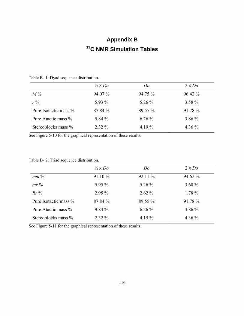
116

Appendix B 13C NMR Simulation Tables

Table B- 1: Dyad sequence distribution.

½ X Do Do 2 X Do

M % 94.07 % 94.75 % 96.42 %

r % 5.93 % 5.26 % 3.58 %

Pure Isotactic mass % 87.84 % 89.55 % 91.78 %

Pure Atactic mass % 9.84 % 6.26 % 3.86 %

Stereoblocks mass % 2.32 % 4.19 % 4.36 %

See Figure 5-10 for the graphical representation of these results.

Table B- 2: Triad sequence distribution.

½ X Do Do 2 X Do

mm % 91.10 % 92.11 % 94.62 %

mr % 5.95 % 5.26 % 3.60 %

Rr % 2.95 % 2.62 % 1.78 %

Pure Isotactic mass % 87.84 % 89.55 % 91.78 %

Pure Atactic mass % 9.84 % 6.26 % 3.86 %

Stereoblocks mass % 2.32 % 4.19 % 4.36 %

See Figure 5-11 for the graphical representation of these results.

117

Table B- 3: Tetrad sequence distribution.

½ X Do Do 2 X Do

mmm % 90.00 % 90.45 % 93.40 %

mmr % 2.99 % 2.55 % 2.29 %

mrm % 1.49 % 1.34 % 0.91 %

mrr % 2.49 % 2.66 % 1.6 %

rmr 1.49 % 1.20 % 0.90 %

rrr % 1.49 % 1.80 % 0.89 %

Pure Isotactic mass % 87.84 % 89.55 % 91.78 %

Pure Atactic mass % 9.84 % 6.26 % 3.86 %

Stereoblocks mass % 2.32 % 4.19 % 4.36 %

See Figure 5-12 for the graphical representation of these results.

Table B- 4: Pentad sequence distribution.

½ X Do Do 2 X Do

mmmm % 89.04 % 89.40 % 92.85 %

mmmr % 1.49 % 1.32 % 0.89 %

mmrm % 1.87 % 1.97 % 1.36 %

mmrr % 1.46 % 1.29 % 0.89 %

mrmr % 1.50 % 1.30 % 0.89 %

mrrm % 0.50 % 0.40 % 0.45 %

mrrr % 1.45 % 1.70 % 0.89 %

rrmr % 1.47 % 1.32 % 0.90 %

rmmr % 0.60 % 0.64 % 0.45 %

rrrr % 0.61 % 0.64 % 0.45 %

Pure Isotactic mass % 87.84 % 89.55 % 91.78 %

Pure Atactic mass % 9.84 % 6.26 % 3.86 %

Stereoblocks mass % 2.32 % 4.19 % 4.36 %

See Figure 5-13 for the graphical representation of these results.