active optics: a new technology for the ...itek 77-0067-1 sll 80 293/ao copy 1 active optics: a new...

Itek 77-0067-1

SLL 80 293/AO copy 1

ACTIVE OPTICS: A NEW TECHNOLOGY

FOR THE CONTROL OF LIGHT

by

John W. Hardy

Itek Corporation, Optical Systems Division, 10 Maguire Road, Lexington, Massachusetts 02173

June 1977

Invited Tutorial/Review Paper for publication in

PROCEEDINGS OF THE IEEE ÄJ&Severi fat SftibÜe reieaMJ FJtälts.tteti öaän&Etftd

Optical &

19980309 342

DTIC QUALITY IKSPHOTB $

PLEASE RETURN T0:

BMD TECHNICAL INFORMATION CENTER BALLISTIC MISSILE DEFENSE ORGANIZATION

7100 DEFENSE PENTAGON WASHINGTON D.C. 20301-7100

u^iozy

Accession Number: 4102

Publication Date: Jun 01,1977

Title: Active Optics: A New Technology for the Control of Light

Personal Author: Hardy, J.W.

Corporate Author Or Publisher: Itek Optical Systems, 10 Maguire Road, Lexington, MA 02173 Report Number Assigned by Contract Monitor: SLL 80-293

Comments on Document: Archive, RRI, DEW

Descriptors, Keywords: Active Optics Technology Control Light Tutorial Wavefront Sensing Technique Measurement Correction Device Random Disturbance Bragg Cell Segment Mirror Monolith Membrance

Pages: 110

Cataloged Date: Dec 10,1992

Document Type: HC

Number of Copies In Library: 000001

Record ID: 25674

Source of Document: DEW

Itek 77-0067-1

PFR-77-067

ACTIVE OPTICS: A NEW TECHNOLOGY

FOR THE CONTROL OF LIGHT

by

John W. Hardy

Itek Corporation, Optical Systems Division, 10 Maguire Road, Lexington, Massachusetts 02173

June 1977

Invited Tutorial/Review Paper for publication in

PROCEEDINGS OF THE IEEE

Optical Systems

Copyright® 1977 Itek Corporation

ABSTRACT

Active optical systems are those in which real-time control over optical wavefronts is employed to optimize system performance in the presence of random disturbances. Applications include (1) outgoing-wave systems for maximizing the power density of a laser beam on a target and (2) received-wave systems for maximizing the angular resolving power of a telescope viewing a distant object through a turbulent atmosphere.

In this tutorial/review paper, the basic concepts of active optics systems and their historical evolution are discussed, from early figure-control systems with a servo bandwidth of less than 1 Hz to the recently developed high-bandwidth systems for atmospheric compensation with bandwidths of several hundred hertz. A critical comparison of the various approaches to wavefront sensing is then made covering both coherent (laser) and incoherent (white-light) systems. Current techniques for wavefront correction, including Bragg cells, segmented mirrors, thin-plate deformable mirrors, monolithic mirrors, and membrane mirrors are described. The performance analysis and optimization of closed-loop systems is covered using two basic models. The paper concludes with a review of the design and performance of five current experimental active optical systems, with some comments on future applications.

CONTENTS

I. Introduction 1

II. Background 9

III. Wavefront Sensing Techniques 15 A. Direct Wavefront Measurement Systems 16 B. Indirect Wavefront Measurement Systems 36

IV. Wavefront Correction Devices 45

V. System Considerations 82

VI. Applications 92

VII. References 107

2. 3. 4. 5. 6.

11. 12.

FIGURES

Optical Image Intensity Distributions for Circular Apertures and Square Apertures o Wavefront Aberration Function 4 Basic Active Optics Systems ."'*'.' 6 Monochromatic Wavefront Sensors 18 Narrow-Band Wavefront Sensors . . 21 Phase Contrast Vector Diagram 03

7. Shearing Interferograms Produced by a Double-Frequency Grating With Two Orthogonal Sets of Lines 26

8. White-Light Wavefront Sensors '.'.'. 28 9. Hartmann Wavefront Sensor 30

10. Hartmann Wavefront Sensor, Image Plane Spot Distribution . . . . . '. . . . \ 31 Imaging Hartmann Sensor Model . . . '',' ' 33 Sidebands Produced by a Symmetrical Square Wave Grating . . . . . 34

13. Wavefront Reconstruction From Phase Difference Measurements 37 14(a). Wavefront Reconstruction Algorithm . ! '. 38 14(b). Mechanization of Wavefront Reconstruction Algorithm Using Analog

Computer 15. Multidither COAT System With Different Sinusoidal Tagging

Frequencies Applied to Phase Shifters 40

Multidither Phasor Diagram 40 Multidither COAT System Spectral Components 42

18. Electro-Optic Wavefront Corrector Using Bismuth Silicon Oxide Crystal

19. Bragg Cell '.'.'.'. '. . . . . \ \ ..'..... \ \ \ 43 20. Operating Regimes for Active Mirrors 50 21. Types of Active Mirrors r1

22. Three-Segment 56-CM Diameter Active Mirror '.'.'.'.'. 53 23. Actuator Force Array Locations on Thin Deformable Mirror [ 55 24. Single-Actuator Control Model for Thin Plate Mirror . . . 57 25. Nyquist Plot for Two-Actuator System 57 26. Mirror Control System With Decoupling Network '.'.'.'.'. m 27. Driving Force Configurations Required to Obtain Displacement at

One Actuator Only in a Thin-Plate Mirror . 60 28. Piezoelectric Actuator Device 29. Inchworm Device „, g4 30. Inchworm Displacement Versus Time ,. 31. Force Actuator for a Large Primary Mirror. '.'.'.'.'.. 65

VI

16. 17.

32. Bending Moment Actuator 68 33. Schematic Diagram of Thin Plate Telescope Mirror With

Active Figure Control 68 34. 76-Centimeter Deformable Mirror Assembly 69 35. Thin-Plate Active Mirror With Piezoelectric Position

Actuators 70 36. Beryllium 37-Actuator Deformable Mirror Using PZT Stack

Drivers 71 37. Influence Function Profiles of Beryllium Mirror 71 38. Construction of Monolithic Piezoelectric Mirror (MPM) 73 39. MPM Response Function 75 40. Monolithic Peizoelectric Mirror 76 41. Interferograms Showing Controlled Surface Deformation of a

Monolithic Piezoelectric Mirror 77 42. Membrane Mirror With Electrostatic Drive 78 43. First System Model—Received Wavefront Compensation 83 44. Wavefront Fitting Error for Atmospheric Turbulence With

Various Mirror Response Functions 86 45. Second System Model—Outgoing Wave Multidither System 89 46. Multidither COAT System Block Diagram 94 47. Multidither COAT System Beam Width Profiles in High Turbulence 94 48. Real-Time Atmospheric Compensation (RTAC) System Block Diagram 97 49. Relationship of Wavefront Sensor Detectors to MPM Actuator Locations

in 21-Element RTAC System 98

50. Optical Assembly of RTAC 99 51. Complete RTAC System Mounted on 1.55 M (61-Inch) Telescope at

Harvard Observatory, Harvard, Mass 100 52. RTAC System Test Data !0i 53. Two Frames From a 15-MM Movie Showing Operation of RTAC Over

a 300-Meter Turbulent Path, Using a 30-CM Aperture Corrected by the 21-Zone RTAC 102

54. RTAC Performance With an Extended Image, Using a 3-Bar Resolution TarSet 103

55. Block Diagram of Image Sharpening System 104 56. Images of Sirius Recorded With the Image Sharpening System 104

VII

TABLES

1. Classification of Active Optical Systems 11 2. Wavefront Sensing Techniques 17 3. Properties of Optical Faceplate Materials 53 4. Characteristics of Lead Titanate Zirconate Piezoelectric Materials 62 5. High Bandwidth Active Mirrors 81

VIII

I. INTRODUCTION

Active optics is a general term for optical components whose characteristics are controlled during actual operation, to modify optical wavefronts. The simplest active optical systems are those controlling focus and tilt; they range in complexity up to systems employing deformable mirrors which may possess more than a hundred degrees of freedom. The concept of active optics has been in existence for perhaps 25 years; the technology that is now emerging is expected to have a profound effect on the design of future high-performance optical systems.

Over a span of 700 years, since the first recorded use of optical lenses as eyeglasses for the correction of sight in 13th century Italy, optical technology has been based on the use of fixed optical components such as lenses, mirrors, and prisms. Following the invention of the telescope 300 years later, the instrument makers of the next centuries were able to build telescopes and microscopes of increasing perfection that provided ever more revealing glimpses of previously unknown macroscopic and microscopic worlds. Much of man's present knowledge of the universe has been gained with optical instruments such as refracting and reflecting telescopes, the spectro- scope, the microscope, and the camera. Modern instruments employ a highly developed optics technology using special glasses, aspheric surfaces, and multilayer dielectric coatings, yet most have one basic feature in common with the 13th century eyeglass—the use of fixed optical surfaces.

The reasons for the historical use of rigid optical components are clear: the visual spectrum is centered on a wavelength of about half a micrometer; lens and mirror surfaces must be figured to control optical wavefronts to a quarter wavelength or less to obtain good image quality. The straightforward solution to this problem is to make the surfaces from a rigid material such as glass, worked to give the required shape, and then to rely on the dimensional stability of the material to provide acceptable performance during the life of the device.

While fixed optical elements are satisfactory for the majority of applications in which the operating conditions can be controlled or at least adequately specified, there is an increasing number of applications in which environmental stress and random processes may dominate the performance of an optical system. Current examples of such applications are: 1) large ground- based telescopes whose angular resolving power is limited by atmospheric turbulence, 2) large telescopes orbiting in space which suffer varying thermal and gravitational stresses, and 3) optical systems for high-energy lasers whose wavefronts are deformed due to thermal effects in the components or in the propagation path.

The performance and reliability of many functional systems can be vastly improved by the use of closed-loop feedback systems. It is interesting to note that most living creatures rely on feedback in their nervous and motor systems to perform everyday functions. Many animals, including man, rely on an adaptive optical imaging system for their eyesight, using a flexible lens of variable focal length, operated by muscular power and controlled by signals from the brain, the system functioning as a closed loop to maximize the acuity of the image on the retina. We know that flexible lenses are not essential for controlled focus; it can be done by moving rigid

lenses. The point is that active optical devices have evolved in nature; after 700 years of developing conventional rigid optics, man is just becoming conscious of the possibilities.

This tutorial/review paper is intended as a general introduction to active optics. As an aid to achieving that goal, an attempt has been made to systematize the various approaches and devices that have been scattered through the literature in this rapidly developing field and to present them in a logical context. The main emphasis is on practical systems and the devices required to implement them.

The paper is organized as follows: the motivation and basic concepts of active optics are discussed in the Introduction; Section II reviews the historical background to active optics, summarizes the major problems and applications that are receiving current attention, and briefly reviews the many different approaches and technologies being presently applied.

In the following sections, the major areas of active optics technology are reviewed in turn: Section III treats wavefront sensing techniques, and Section IV covers wavefront correction devices. The major considerations in system design are summarized in'Section V. A review of the present and some possible future applications is contained in Section VI. The list of references in Section VII is intended to provide comprehensive coverage of the material presented.

The control of wavefronts is essential in optical systems that collect and concentrate energy either to obtain a sharp image as in a telescope, or to produce a high power density in a specific location as in laser systems. This concentration of power involves the generation of spherical wavefronts that converge to a point. The allowable deviation from sphericity is very small, as will be shown.

For analysis of image structure, geometrical optics loses its validity and the intensity distribution in the vicinity of the image must be determined by diffraction theory. It is well known that the amplitude distribution of the light in an image plane is the two-dimensional Fourier transform of the phase and amplitude distribution at the aperture (17). For a perfect wavefront (a constant amplitude sphere), a square aperture produces a (sin x2/x) intensity distribution, whereas a circular aperture produces a (2 Jtx2/x) intensity distribution, the familiar Airy diffraction pattern. These basic image intensity distributions and their parameters are shown in Fig. 1. Wavefront aberrations in the aperture cause a redistribution of power in the image. For small phase aberrations, the most noticeable effect is a reduction in peak intensity; for large abberations the structure of the image is degraded.

The imaging system model (Fig. 2) shows a wavefront with an aberration function $ in relation to the spherical reference surface S. At a location Q, the wavefront may be described as Aeik($+ R), where A is the amplitude and R the radius of the reference sphere. The disturbance at a point P on the optical axis at the image plane is

u(P) = -{^^ JJ\-M*+R)dS

,2, where dS = a p dp dö is an element of the reference sphere S and a, p, and 9 are defined in Fig. 2.

The intensity at point P is then

HP) = IU(P) i'= (^)! n Jo Jc

2v eik* p dp d6

ti

"jF FiJ-l n, 100 HflVFS

Fig. 1 — Optical image intensity distributions for circular apertures (left) and square apertures (right). The top pair represent perfect optical systems with no wavefront aberration. The middle pair depict the intensity distributions for small aberrations (0.1 wave rms), showing a reduction in peak intensity but little change in shape. For larger aberrations (0.3 wave rms) the structure of the image is changed

Aberrated wavefront

Spherical reference surface S

a2p dp d0

Fig. 2 — Wavefront aberration function. The ideal wavefront for a diffraction limited system is the spherical reference surface S. The wavefront aberration function <i> at point Q is the difference between the aberrated wavefront and the surface S. The resulting disturbance at image point P is obtained by integrating the aberrated wavefront over all elements of the wavefront, dS

This intensity may be normalized to that of an unaberrated system.

If # = 0 ,2\2 1 -* Uv

The normalized intensity is then

,2ir

1(P) ~ I* ~ 7T2 J7 eik* p dp d6>

0

i(P) is a commonly used figure of merit known as the Strehl ratio (12a), describing the ratio of the actual peak intensity of an image to that of a perfect unaberrated system.

If the wavefront aberrations are small (A<p < A/10), the peak intensity may be written (12b)

i(P) ~ 1 " (y) 2 <**)2

where (A*)2 is the mean square error of the wavefront [ $p - ($p)2]. The normalized intensity at the focus is therefore independent of the nature of the aberration, enabling wavefront quality to be specified in terms of the variance from the reference spherical wavefront.

For an rms error of 0.1 wavelength

A* A = 0.1 i(P) ~ 0.60

The extreme sensitivity of the image peak intensity is therefore demonstrated, as only one-tenth wave rms error will reduce the peak intensity to 60 percent of the ideal. For many applications this is an unacceptable loss of intensity, and provides the motivation for the use of active optical systems.

The purpose of an active optical system is to optimize a desired property of the system such as the energy density in a specific location. Three basic components are required: a wavefront-modifying device, which may be reflective or refractive; a measuring device that accepts light and provides an output related to the property being optimized; and an information-processing device that accepts the measured data and converts it into the appropriate control signals for the wavefront-modifying device.

The arrangement of these basic components depends on the purpose of the system. Four typical active optical systems designed to correct random wavefront distortion are depicted in Fig. 3. The source of this distortion may be turbulence in the propagation path, aberrations in the optical system, or a combination of both.

The first two block diagrams represent transmitted wavefront systems, in which the objective is to maximize the power density at the target. Such systems normally operate at a single wave-- length, using radiation generated by a laser. In the phase conjugation approach, the beam initially reaching the target gives rise to reflection from small areas producing glints which generate spherical waves. These reflected waves traverse the propagation path in the reverse direction and consequently are spatially modified by the turbulence in the same was as the transmitted beam.

Transmitted Wavefront Systems

////

Source

"7 4^ Wavefront modifier

Wavefront detector

Glint

Wavefront processor

/ Optical path disturbance (OPD)

(a) Phase conjugation OPD Glint

Source Aperture tagger

Wavefront modifier

1 -Jl ~^WT~ Target

J 1 < / Intensity /\y detector Wavefront

processor

(b) Aperture tagging

Received Wavefront Systems

OPD

V Wavefront modifier Image

detector

Wavefront processor —

Wavefront detector

(c) Wavefront compensation

OPD

Aperture — Wavefront

tagger modifier

Wavefront proce ssor

V Image detector

Intensity detector

(d) Image sharpening

Fig. 3 — Basic active optics systems

The received wave is compared with a locally generated reference wave in the wavefront detector and the required correction, which is the phase conjugate of the measured wavefront distortion, is computed in the wavefront processor. A command is then sent to the wavefront modifying device to implement the required correction in the transmitted wavefront. The predistortion impressed on the outgoing wavefront then precisely compensates for the distortion in the propagation path so that the wavefront arriving at the target has the desired spherical shape to maximize the power density at the original glint. In practice, the performance of active optical systems depends on such factors as the error in the wavefront measurement, the response time of the system, and the precision with which the wavefront can be modified.

The second transmitted wavefront system is the aperture tagging approach in which trial perturbations are made in the outgoing wavefront and the optical power returned from a glint at the target is analyzed to determine which perturbations increase the power density. These perturbations are added to the wavefront and the process continues iteratively until the power density is optimized. This operation is known as "hill climbing" because the servo control loop is con- stantly seeking to maximize some figure of merit such as power density. The process has been likened to a lone climber trying to find the highest peak of an unknown mountain range in a snow- storm, armed only with an altimeter. This description is overly pessimistic because hill-climbing systems using aperture tagging have been successfully operated; however, it does point up the potential problems of the approach. The main differences between aperture tagging and phase conjugation are: (1) In the former, the trial perturbations must be uniquely separated (i.e., tagged) in time or frequency; as a result, the system frequency response becomes increasingly limited as the number of independent aperture modes increases. In the phase conjugation approach, the wavefront in each section of the aperture is separated spatially and may be measured independently so that system performance is not significantly influenced by the number of degrees of freedom in the aperture. (2) With aperture tagging, the radiation from the glint that is picked up by the detector does not traverse the same optical path as the outgoing radiation. This is considered an advantage in high-energy systems when nonlinear effects due to thermal blooming may occur in the outgoing beam.

The second pair of block diagrams represent received wavefront systems in which the objective is to obtain the best possible image of a distant objective viewed through a turbulent atmospheric path. An obvious example is a ground-based astronomical telescope looking through the earth's atmosphere. The objects viewed are self-luminous, producing incoherent radiation over a wide spectral band.

The first of these techniques is known as wavefront compensation and is analogous to the phase conjugation approach in laser transmission systems. The object being viewed may be regarded as a collection of unresolved point sources, each one generating a spherical wave, which is distorted in its passage through the turbulent atmosphere. After collection by the telescope aperture and passing through the wavefront modifier (assumed to be initially nulled) the distorted wavefront is split in intensity and a portion is sent to the wavefront detector to be analyzed in terms of the local deviation or tilt from the ideal spherical wave. In this way a complete error map of the received wavefront is generated; the required correction is then computed in the wavefront processor and the necessary control signals for each local area of the aperture are sent to the wavefront modifier. The wavefront error is consequently nulled at the input to the wavefront detector, so that the optical beam reaching the image detector is essentially diffraction limited. The actual performance of such a system depends on many factors such as the signal- to-noise ratio of the wavefront detection process, the speed of the compensation loop in relation to the rate at which the atmosphere is changing, and the spatial resolution of the measurement and compensation functions in relation to the wavefront distortion.

The image sharpening technique uses a totally different approach, analogous to aperture tagging. Trial perturbations are made in the received wavefront and the effect is judged by means of a detector located in the image plane, the criterion being to maximize the integral over the image

7

plane of the square of the image intensity, or some related quantity. This is an indirect technique in that some way of reliably distinguishing or tagging the individual aperture perturbations is required; the same limitations with regard to operation with large apertures (requiring a large number of degrees of freedom) obtain with this system as with outgoing wave aperture tagging systems. Image sharpening systems require only a single detector channel, giving them a practical advantage when the number of degrees of freedom in the wavefront modifier is small, or when there is adequate time for computing the wavefront correction as in the case of mirror figure control system.

n. BACKGROUND

The earliest recorded use of active optics is probably Archimedes' use of a "burning glass" to set fire to the approaching Roman fleet as they sailed into Syracuse Harbor in 215 BC (2). It is hard to imagine this feat being performed by a single optical lens; it has been speculated that the burning glass may in fact have been an array of polished metal mirrors, each one directed by a man (30, 31).

The principle of using moving mirrors to capture the sun's radiation is of considerable importance in these energy-conscious times. The U.S. Energy Resources Development Agency (ERDA) is working on an experimental steam generating plant near Albuquerque, N.M., using a field of mirrors that track the sun and direct the energy to a central boiler mounted on a tower (42). Plans have recently been announced for a similar installation at Barstow, California, which will have 10 megawatts of electrical generating capacity.

The solar furnace of the French National Center for Scientific Research at Odeillo in the Pyrenees has been in operation since 1970. An array of 63 flat mirrors with a total area of 2592 square meters tracks the sun and directs the radiation to a large fixed parabolic mirror which concentrates the power, normally amounting to 1000 kilowatts, into a furnace in which temperatures of 3800°C have been obtained (53).

These examples of multi-mirror systems are non-coherent; no attempt is made to match the phases of the wavefronts reflected from the individual elements. The size of the final image is governed by the size and quality of the individual mirrors, while its intensity is equal to the sum of the individual image intensities. As will become apparent in the following sections of this paper, the prime motivation for using active optics, providing both the biggest payoff in terms of performance and the greatest technical challenge, lies in the development of coherent active optical systems. To achieve a useful degree of coherence, the rms phase error across the wavefront should not exceed about 1 radian, which corresponds to a path length error of about 10"7 meters (1000 A) at the peak visible wavelength. The required position accuracy of a mirror surface at normal incidence is one-half of this value.

A multi-mirror telescope for the collection of radiation from distant astronomical objects is under construction at the University of Arizona (24, 25). This telescope consists of a ring of six circular mirrors on a steerable mount, each mirror 1.8 meters in diameter, with a total light- gathering capability equivalent to a single telescope of 4.5-meter diameter. This instrument may be regarded as transitional between a non-coherent "light-bucket" and a fully coherent synthetic aperture. Its prime use will be at IR wavelengths in the range from 10 to 20 micrometers, where the alignment precision of the individual mirrors allows coherent addition of the wavefronts to provide an angular resolution of 0.5 arc-second. At visible wavelengths the instrument will function as six parallel telescopes, giving a sixfold improvement in light-gathering power but no improvement in resolving power over a single element.

At this point it will be useful to provide some definitions and to categorize the various classes of active optical systems. The terms "active optics" and "adaptive optics" have been used somewhat interchangeably in the past; there is, however, an important distinction to be drawn and the following definitions are proposed: '

• ^ active optical system includes one or more wavefront-modifying components that are controlled in real time, during operation, by internal or external means.

• ^ adaptive optical system is an active system in which the control algorithm is modified in real time as a result of operating experience, in order to optimize system performance.

According to these definitions, active optical systems are the broadest category and include both open-loop and closed-loop control systems. Adaptive optical systems are a restricted category in which performance measurements are made during operation to provide a learning capability.

Active optical systems may be classified according to the degree of control exercised on the wavefront, as measured by the order of a polynomial representation of the wavefront modification function. Table 1 shows such a classification. The most elementary active optics systems are those in which the wavefront is axially displaced, without further modification; the conventional focusing system used in most cameras in which a lens or lens component is moved axially is a typical example. Piezoelectrically controlled mirrors for varying the length of laser cavities and interferometer paths also belong to this class.

First-order systems produce a wavefront tilt; typical examples are:

• Tracking and scanning mirrors with control of the tilt angle using electromagnetic or piezoelectric actuators,

• Scanning mirrors with resonant drives for systematic optical scanning,

• Rotating multi-faceted mirrors as used in optical scanners,

• Acousto-optic cells using Bragg or Raman-Nath diffraction to change the direction of propagation of a light beam.

Second-order active optics systems are those in which the radius of curvature of the wavefront is changed, controlling the effective focal length. This operation normally produces a change in both the image size and image position. Zoom lenses are designed to change the size of the image while maintaining the image plane in a fixed position by simultaneous movement of the exit pupil to compensate for the change in focal length. Such lenses are now common in cameras and projectors Methods for altering the perspective of optically projected images using variable anamorphic lenses have been described by Hemstreet (6), and a system for correction of geometrical image distortion using zoom and anamorphic lenses with closed loop control was described in 1968 by Hardy (16). These systems all employed rigid optical surfaces.

A forerunner of contemporary deformable mirrors was the varifocal mirror described by Muirhead in 1961 (7), which consisted of a metalized Mylar membrane stretched taut over a circular frame. Variation of the relative air pressure between front and back of the membrane varied the curvature, and therefore the focal length, of the mirror. This principle was used in 1967 by Traub (15), who employed a loudspeaker cone to drive the membrane at frequencies up to 60 Hz to generate a three-dimensional display from a cathode-ray tube image.

Second and higher order active optical systems can be divided into two major types depending on whether the wavefront modification is implemented systematically (describable in terms of mathematical functions of ascending order) or zonally (as an array of independently specified values). The classic optical aberrations of defocus, spherical aberration, astigmatism, and coma,

10

Table 1 — Classification of Active Optical Systems

Order of System Wavefront Function

Equation Description

Application

Z = a Uniform (axial) displacement

(1) Plane wave

(2) Converging beam

Interferometers, optical cavities

Focus control

Z = ab+by Wavefront tilt

(1) One-dimensional Optical scanning, image motion compensation

(2) Two-dimensional Optical tracking, image positioning

N

Z = ax2+by2

j,k=N

z=EaixV j,k=0

Radius of curvature

(1) One-dimensional Anamorphic magnification,

perspective change

(2) Two-dimensional Zoom lens varifocal lens

General two-dimensional disturbance

Correction of random aberrations, atmospheric compensation

11

which have considerable symmetry, are readily describable systematically in terms of low-order Zernike polynomials (12C). However, the description of random wavefronts with a large number of degrees of freedom requires sensibly the same number of coefficients whichever method is employed.

Coherent wavefront modification systems of higher than second order have been the latest to emerge and are now being actively developed for applications such as figure control of large telescope mirrors, real-time atmospheric turbulence correction, and compensation for thermal blooming.

The possibility of compensating for the wavefront distortion due to the earth's atmosphere, which is a major limitation to ground-based astronomy, was discussed in 1953 both by Horace Babcock (1) and by James G. Baker in an unpublished report. Baker pointed out that when observing a single star, compensation for the telescope aberrations and for the atmosphere near the telescope aperture could be made with a single wavefront corrector. He suggested the use of a Foucault test with a bank of photocell receivers to generate the necessary correction signals. When dealing with a wider field of view, covering several stars, the atmospheric correction required is different in each direction and a single corrector cannot be used. Baker proposed solving this problem by re-imaging the entire turbulent atmospheric path within the optical system of the telescope and passing the beam through a refractive gas cell using lateral ultrasonic transducers to introduce density variations along the cell that would compensate for the effects of the phase disturbances at conjugate locations in the propagation path. A digital computer would be used to calculate the required corrections in real time.

Babcock originally proposed the use of an arbitrarily deformable optical element with feedback from a wavefront sensor, suggesting the use of an Eidophor in which the thickness of an oil film on the surface of a mirror is controlled by electrostatic charges deposited by a scanned beam from an electron gun, thereby producing controlled optical phase shifts in the reflected light. A letter published by Babcock in 1958 (5) suggested an improved form of mirror consisting of a flexible reflecting film with an array of target elements on which the electrostatic charge is deposited, thereby producing local bending of the film. There is no record of either of these proposals having been implemented.

In 1956, a first-order active optics system for compensation of image motion in astronomical telescopes was described by Leighton (3). This system, which used an electromagnetically operated tip-tilt mirror with a bandwidth of 5 Hz, was used on the 60-inch reflecting telescope at Mount Wilson Observatory, with the aperture stopped down to 20 inches, and was instrumental in obtaining some spectacular planetary photographs, characterized as the best obtained up to that time.

Due to the difficulty of implementing high-order systems with a speed fast enough to compensate for the atmospheric turbulence, which requires a bandwidth of several hundred hertz, attention in the 1960's was turned away from direct (predetection) compensation of atmospheric turbulence toward post-detection image processing and toward active figure control of large telescope mirrors, especially those intended for use in space, where the control bandwidth is typically less than 1 Hz. The first approach was to use a segmented mirror, as described by Robertson et al. (14) in 1966, each segment being controlled in two axes of tilt and one of focus by three actuators. Because of the difficulty of manufacturing a large number of individual mirror segments, which in the case of an astronomical reflecting telescope are all off-axis aspheric surfaces, attention was directed to the use of thin continuous deformable mirrors. A description of a 76-centimeter, f/3 spherical mirror with 61 force actuators evenly spaced over the rear of the mirror was given by Robertson (21) in 1970. The control system concept and the practical problems associated with actuators for large active mirrors also received considerable attention at this time, as reported by Creedon and Robertson (20).

12

A new technique for deforming flexible mirrors using bending moments within the mirror itself rather than force against a support structure was described in 1975 by Scott (46). A similar scheme was independently proposed by Berggren and Lenertz (47). A more detailed discussion of the development of large active mirrors and the associated figure sensing and control systems is given in later sections of this paper.

The basic techniques of adaptive control over electromagnetic wavefronts are first developed in the early 1960's for use in microwave systems. The self-phasing array antenna described by Skolnik and King (9) is the direct forerunner, at microwave frequencies, of the phase conjugate active optical system of Fig. 3a. The self-focusing receiving antenna (10) uses the same principle of operation as the wavefront compensation system of Fig. 3c. The principle of beam tagging in adaptive antenna systems was described by Adams (11) in 1964, who noted that "the beam tagging process optimizes the received signal at the point where the tagging modulation is analyzed." This principle is used in transmitted-wave aperture-tagging systems (such as multi-dither coherent optical adaptive techniques) generically shown in Fig. 3b, and also in the received wave image- sharpening system of Fig. 3d.

These similarities of system concept do not extend to the actual hardware because of the difference of about 104 between the optical and microwave frequencies, and the greatly differing effect of physical factors on the propagation path. Thus, the development of active optics systems has been gated mainly by the development of suitable hardware rather than by the need to develop system concepts. The main area of commonality is in the information-processing functions, because heterodyne detection is used in both microwave and optical systems to obtain baseband signals for control and information extraction, which may then be handled by conventional analog or digital electronics. The latest major application of adaptive arrays has been in radio astronomy, where there is a need for very large apertures in order to obtain high angular resolution. Because of the large area required, many installations use sampled or sparsely filled apertures in which both the physical location and the phasing of the individual elements can be controlled. Some pre- liminary work has been done on optical arrays using these principles, but because of the much shorter wavelengths involved, there are considerable practical difficulties in maintaining the necessary alignment between individual optical elements.

The development of high-bandwidth active optics systems for real-time atmospheric compensation is quite recent, and many different approaches have been reported. The initial problem attacked was that of maximizing the power density of a laser beam propagating through the turbulent atmosphere. Such systems are generally known as coherent optical adaptive techniques (COAT). The phase conjugation approach described in 1970 by Cathey et al. (23) uses the principle of optical reciprocity in which the phase shift in the return path between a specular reflection (glint) on the target and the transmitter is measured in real time at two or more locations in the transmitting aperture. A compensating phase shift is then inserted at the corresponding location in the aperture to make the transmitted laser wavefront match the wavefront received from the target glint, thereby increasing the power density in the vicinity of the target glint.

A different approach first proposed in 1971 by O'Meara and described by Bridges et al. (35) in 1974 uses the principle of measuring the intensity of the radiation returned from a target glint while making trial perturbations of the transmitting aperture, each section of which is tagged with an identifiable signature. A multi-dither COAT system of this type using an 18-element phase corrector was described by Pearson et al. (59) in 1976. Each controlled element was identified by modulating or "dithering" the phase by about ±30 degrees at a different temporal frequency, within the range from 8 kHz to 32 kHz.

The requirements for wavefront compensation when imaging distant objects such as stars through the atmosphere are quite different, because the object radiance itself must be used as the reference source. Such sources emit a broad spectrum, necessitating measurement and compensation of optical path length rather than phase angle. The first practical system of this type was

13

developed at Itek in 1973 and was described by Hardy et al. (37) in 1974. This real-time atmospheric compensation (RTAC) system used an ac white-light lateral-shear interferometer (34), a parallel analog computer, and a 21-element monolithic piezoelectric mirror (38). Successful operation over a 250-meter horizontal atmospheric path was obtained in 1974. Because of its parallel architecture, the performance of this approach, as measured by the residual wavefront error for a given reference source stellar magnitude, is virtually independent of the order of the system (i.e., independent of the number of corrected subapertures). The RTAC approach therefore is advantageous for large astronomical telescopes over aperture tagging systems, whose performance bears an inverse relation to the number of subapertures, as shown by Dyson (43). A compensated imaging system using the RTAC approach to obtain improved imaging of stellar objects through the earth's atmosphere using large ground-based telescopes is presently being developed under the sponsorship of the Defense Advanced Research Projects Agency (Looft, 1976 (61)).

An image sharpening system using sequential tagging of small sections of the telescope aperture was proposed by Müller and Buffington in 1974 (41), the prime application being for atmospheric compensation of ground-based astronomical telescopes. The authors investigated different image sharpening algorithms and control algorithms using a computer simulation. Practical results for a six-element system of this type over a terrestrial path were reported in 1976 by Buffington et al. (54) and first observatory results of stellar image sharpening were reported in 1977 (64).

In reviewing the progress made in active optics over its period of intensive development in the last ten years, certain trends are already apparent. Wavefront correction devices have progressed from the use of 'lumped" components such as lenses and mirror segments moved in their entirety toward the use of distributed correction using deformable mirrors. The means of control for large active telescope mirrors is likewise evolving from separate piston or position actuators which require a stable reaction plate, toward force and bending moment actuators which do not.

For high-speed active compensation, small deformable mirrors using piezoelectric actuators are presently the most highly developed devices, but from the wide variety of current approaches, described in Section IV, it is difficult to predict what the future will bring.

As regards wavefront sensing techniques, the first figure sensors were based on conventional interferometers using local monochromatic (laser) sources. The trend now is toward ac white- light interferometry using natural sources such as bright stars. For high bandwidth operation such as atmospheric compensation in passive imaging systems, subaperture tagging with serial processing has been used for small apertures, but direct wavefront measurement at the receiving aperture followed by parallel data processing is necessary for large telescopes.

For active laser beam control, both phase conjugation and the multi-dither approach have been shown to be effective.

14

III. WAVEFRONT SENSING TECHNIQUES

A wavefront sensor is necessary in every closed-loop active optics system. The first real- time wavefront sensors to be developed were those for detecting defocus in optical projection systems and tilt-angle errors in optical trackers.

Focus sensors are based on maximizing the irradiance (or some function of the irradiance) of the light reaching the image plane. Suitable criteria for this purpose have been reviewed by Linfoot (4) and by Müller and Buffington (41). Quadrant detectors have been used for sensing of wavefront tilt or angle of arrival in optical tracking systems; improved precision is obtained by optically nutating the beam to produce ac modulation. A rotating mirror sensor for high-resolution optical tracking has been described by Lim and Subramanian (29).

Image position and tilt detectors are low-order wavefront sensors and the basic techniques have been known for some time. High-order wavefront sensors have evolved within the last decade; some of these sensors have adapted low-order techniques to a large number of subapertures, as in the case of the Hartmann imaging sensor, which tracks the positions of multiple images. Others are based on classical interferometric testing techniques for lenses and mirrors, suitably modified for real-time operation.

Real-time wavefront sensing for active optics systems imposes the following special requirements:

a) The wavefront deformations to be measured in active systems are usually random, requiring higher spatial resolution than the measurements generally employed to detect the common optical manufacturing aberrations such as spherical, astigmatism, and coma.

b) The range of optical phase errors over which reliable measurements must be made in an active system may be considerably more than one wavelength, introducing phase ambiguity problems; at the same time, the null phase measurement indicating correction of the wavefront error must be made with precision and reliability. These requirements together imply a large dynamic range. Fortunately, closed-loop feedback systems operate by nulling the error; variations in wavefront sensor linearity influence the loop gain of the feedback system, but not the precision of the null.

c) The illumination of the aperture being measured in an active optics system is often uncontrolled and in the case of systems operating through atmospheric turbulence, there may be large random variations of intensity across the aperture. For this reason it is necessary for an active optics wavefront sensor to be capable of measuring phase independent of intensity. Systems using ac modulation and heterodyne detection provide this capability.

d) Real-time operation implies a limit on the time available to make the wavefront measurement and to process the data; the available time varies from the order of milliseconds for atmos-

15

pheric compensation up to many seconds for figure-correction systems. The required response time may be a deciding factor in the type of wavefront measuring system used in any particular case.

There are many possible ways to classify wavefront sensors, depending upon the viewpoint; for active optics applications it is useful to divide the field broadly into direct and indirect measurement techniques.

Direct wavefront measurement involves determining the point by point phase (or optical path difference) of a received wavefront either by comparing it with a reference wave in the case of coherent systems, or by determining the local slope of the wavefront when the radiation is incoherent and subsequently reconstructing the wavefront itself.

Indirect wavefront measurement requires a control loop and computer; the method is based on making trial perturbations of optical phase in the aperture and observing the image produced by light passing through that aperture to evaluate whether the perturbation increases or decreases a figure of merit related to wavefront error, the process continuing until the error is nulled.

Within these two broad categories there are many different approaches, the most important of which are listed in Table 2. Direct methods can be subdivided on the basis of the useful spectral bandwidth: monochromatic, narrow-band, and wide-band. Indirect systems may be subdivided according to the method of aperture tagging used.

A. DIRECT WAVEFRONT MEASUREMENT SYSTEMS

(1) Monochromatic Wavefront Sensors

The first group of wavefront sensors to be discussed employs the interference of two beams, derived from a monochromatic source, one acting as a reference and the other being modified by the optical path being measured. Optical configurations having the required physical separation of the two paths include the Twyman-Green and Mach-Zehnder interferometers. The allowable path length difference is constrained by temporal coherence of the source to the distance X2/2AX. In practice, because of the difficulty of exactly balancing path lengths, monochromatic light must be used, with low-power lasers that most common source. Apart from coherence problems, double-beam interferometers are sensitive to any disturbance in either the reference or test path, and a precise reference surface, usually a mirror or beam splitter, is required. In addition, there are phase ambiguity problems when the error exceeds 1 wavelength.

A method of increasing the dynamic range of interometric phase measurement by the use of two-wavelength interferometry has been described by Polhemus (33). The two coherent sources at wavelengths Xt and X2 produce an additional fringe pattern superimposed on the interferogram, which is scanned and converted to an electrical signal. This signal is filtered to isolate the low- frequency component, yielding a scanned interference pattern equivalent to that produced by a source of effective wavelength Xeff = X1X2/ \\t - X21. By using pairs of wavelengths with progres- sively smaller spacing, the same interferometer may be used both for initial coarse measurements and for the final diffraction-limited alignment.

Two figure sensors that have been developed under NASA sponsorship for space telescopes are shown in Figs. 4a and b.

The first scheme uses a beam focused at the center of curvature of the primary mirror; in the case of a Cassegrain configuration this is outside of the secondary mirror so that the wavefront sensor can be located where it does not cause significant obscuration of the telescope primary mirror. The interferometer is of the Twyman-Green configuration, modified by the addition of an optical frequency shifter which produces temporal modulation of the fringe pattern and enables an

16

XS ai n S a u •iH O o

O CD o

s o

o S o

o o o

0<J

o CD •a CD

"O CD

§ § T-T o '1 % %

•3 P< co

^ O a CD

1 -4-> a CD

CD

CD

s CD

r-4 53 53 a 55 Al 53 53 CM ■*

1 P W CO CD

1 ^ ö CD CD CD CD CD CD o o u P< P< Pi Pi Pi

a X! u

-*-* ü •f-H 3 3 B 3 3 « /i^ 3 CD u CD

Pi CD

Pi CD

Pi CD

Pi CD

5t Pi CD CD

O s a £ a < S a

< a <

bO S

•iH

Pi <t>

CD CD CD CD CD W CD a a>

Pi rt PI rt

täl 1 a0

Pi rt

■B ■a ■B -H CD U o a o o o Ö s 3 PI ™ Pi Pi Pi o to 'S s ® £

"H m <*H «IH •M JL( d ni « S, CD CD CD CD CD CD

CD {3 CD > M 11 53 *-a 5§ & J ni O ni O Ctf O

ä A ^■a ^■g, ^^ ^ M ^ "co

1 Pi

-Ö a Ä a 5 a a a Ä ö £

V O bO O bD O hß O ho O hD CD

r—1

■s

ft

CD

CD > U CD CO

s

)

M

odul

ati

(26)

ph

ase

an

1.

M

odul

ati

phas

e an

Fri

nge

inte

nsit

y

al.

M

odul

ati

phas

e an

Mod

ulat

i ph

ase

an

Imag

e po

siti

on

1.

M

odul

ati

phas

e an

i

a CD U CD

4H

o> - d ^■^ ^—^ ni

^ o s a

-4-J CD

CO

o in

CD

CD

CO Pi

CM CO CD

>> CD Sä

Pi PI •i-l

CD ^

CD O >. u w W 3 P ft 3 ^ wS

Ex -4-> >> 13 S" 03 H o

Pi +-> CD

bO 3

CO ni p<

Pi

äs Pi &D a s CD *ri •iH

+->

PI

u a ni o

'S" PH ■a » 8

5 i

eral

shi

-f

requ

e ti

ng cti

1 ^ m Pi -I M

u CO CD

P -*-)

ni ® u p}

a) O co O g CD

F W 13 fi •iH P)

a S3 U CD Pi

■b> CD

an CD rj N "ft

■a CD "8 ° rt

J B » i u CD P<

ni a o Pi

o s o

p< w

-t-> > O P< CD CD

■^ CO

P ^

CD O

-(-> ni

c3 ^< EH h

bo g S CD

CH «H a

CD

CD I a

CO CO

s <D Q, I! a -«a M CO

H <« a

Pi Pi CD CD Ä XI

f a0 1 »F-l

S -a ■a CD

i >

ä bß & s 1 8

3 u

1 s

CD T3

is a s a ™

CO

8 CD Q,

IS a -c ö CO

CD W £

C^g g

rt J2 +-> ■a CD

rn rt ni CD

& ^ S Pi bp a. CD

§ p l—l .—s 3 I-1

pq So o m §21

bß a •a CD CD

17

Laser

Optical frequency shifter V//////A Reference flat

(a) Twyman- Green interferometer modified for ac measurement

99.99% Laser

] Modulator

(b) Zone-plate figure sensor with ac operation

Mixer

Phase detector

(o)f - u>r)

IF Detector 1

, w'

Voltage controlled oscillator

cor

~\!gj .

iur

Laser

±_ Bragg cell

^~

J^L, Bragg cell

\ M:j

Bragg cell

Bragg cell

(c) Phase conjugate COAT system

Target

Fig. 4 — Monochromatic wavefront sensors

18

ac heterodyne phase detector to be used (18). In operation, the beam from the laser is expanded and is divided into two beams of approximately equal intensity by the beam splitter. The first (transmitted) beam is focused precisely at the center of curvature of the mirror under test, expands to strike it normally, and is then reflected back on its path to the beam splitter, which now reflects it to the detector plane D. The second beam, initially reflected from the beam splitter, passes through an optical frequency shifter and is reflected back on its path by the reference flat, travelling again through the optical frequency shifter and beam splitter to reach the detector plane D where it interferes with the first beam. If no optical aberrations are present, and if we ignore the frequency shifter for the moment, the two wavefronts reaching D will be plane and parallel, producing a uniform intensity across the plane.

I = It + I2 + 271^2 cos 0

where lu I2 are the intensities of the two beams and <j> is their relative phase shift.

If the mirror under test has aberrations, then the beam reaching D reflected from the mirror will no longer be plane, resulting in a variation of 0 and consequently a variation of intensity across the detector plane. The absolute value of the intensity at any point in the detector plane, !(x,y), depends not only on the phase difference between the optical beams <£(x,y) but also upon their individual amplitudes It and I2, which may also vary across the aperture. The effect of intensity variations is minimized in static interferograms by tilting the reference flat so that the interfering beams are no longer parallel. The phase difference then varies linearly across the detector plane, producing uniform parallel fringes perpendicular to the direction to tilt. Wave- front aberrations displace these fringes; the displacements are detected by* scanning the interferogram across the fringes and recording the position of the center of each dark line. The wavefront aberrations producing the fringe displacements are then readily computed. This process is a spatial phase measurement and the sequential scanning takes time.

The speed of measurement can be increased and the effect of beam intensity variations can be minimized by producing a temporal modulation of intensity in the detector plane, allowing the temporal phase to be measured simultaneously at some or all locations on the wavefront. This effect can be achieved by offsetting the optical frequency of one of the interfering beams by an amount o> so that the measured phase becomes (cot + 0). The frequency offset could be produced by moving the reference flat along the beam axis, thereby producing a Doppler shift. In a practical system, a shift produced in this way would have to be cyclic.

An elegant method of producing a continuous frequency offset is described by Crane (19), using two quarter-wave plates, one fixed and one rotating, through which the reference beam passes twice due to reflection. If the rotation frequency of the moving plate is wq, then the optical frequency of the reference beam after passing through the plates twice is shifted by 2coq, producing a sinusoidal modulation of the intensity of the interference fringes over the entire detector plane D at a frequency of w/ir Hz. The phase of the intensity modulation at any point x,y in the detector plane is then (2wq + 4>x>y). The phase of the intensity modulation at a fixed reference location may similarly be expressed as (2wq + <£r).

By the use of photosensitive detectors in plane D, the optical intensity modulation is converted to electrical signals at frequency «A Hz. Electrical phase detectors are then used to measure the phase difference (^ - 0r) to a high degree of accuracy, unaffected by wide variations of intensity. This measurement may be carried out in all parts of the aperture simultaneously, by using the appropriate number of detectors and phase measuring channels.

A limitation of the laser interferometer just described is the fact that it monitors the figure of only the primary mirror of a telescope. In the second example described (26), shown in Fig. 4b, the laser beam traverses both the primary and secondary of a Cassegrain telescope, enabling errors in the whole optical system to be monitored. The laser beam is folded by a beam splitter

19

and is brought to a focus near the telescope image plane; it then expands to fill the secondary and primary mirrors. Normally the entire beam would be collimated and would exit the aperture. A weak circular zone pattern is applied to the primary mirror so that a small percentage of the light (0.01 percent) reaching the primary is diffracted back into the secondary to form a conjugate image of the laser source close to the original focus. This return beam is folded by a beam splitter and expanded to fill the detector plane D. The reference beam passes directly through the two beam splitters and is similarly expanded so that it superimposes the first beam producing an interference pattern. An optical frequency shifter in the reference beam produces ac modulation of the fringes to enable heterodyne phase detection. The zone pattern impressed on the primary mirror produces a very small amount of scattered light, causing a negligible reduction in image contrast.

The third monochromatic wavefront sensor system shown in Fig. 4c depicts the phase conjugate COAT system (23, 63) in which phase errors due to atmospheric turbulence in an outgoing wave system operating at 10.6 micrometers are corrected in real time. The optic phase shift between a small glint at the target and each section of the aperture is measured using an ac heterodyne interferometer. The appropriate phase correction, which is the conjugate of the measured phase, is then inserted in each section of the aperture to ensure that the wavefront arriving at the target is perfectly spherical, thereby maximizing the peak power. The active elements used in this system are Bragg cells and perform a dual function; they provide the ac modulation of the received signal by virtue of the Doppler shift induced by the acoustic waves in the cells and they also provide the phase shifting function in each channel, as described in Section IV.

Each Bragg cell is driven by a voltage controlled oscillator (VCO) at frequency wi. The received wave in each channel, returned from the target glint has passed through the corresponding Bragg cell twice and is therefore shifted in frequency by 2u>i.

A reference wave shifted by 2wr is generated by a further Bragg cell and plane mirror as shown. The signal in each channel is combined with the reference by means of a beam splitter and is directed to the detector, which produces electrical outputs at the sum and difference frequencies 2N(w! ± wr). In the system described, the channel frequencies are 18 MHz and the reference frequency is 15.75 MHz. The difference frequency (wt - wr)/n = 4.5 MHz is filtered out and its phase compared with that of a local oscillator at the same frequency to produce a dc signal proportional to the phase difference in each channel. To close the control loop, these dc signals are applied to the VCO's that adjust the frequency driving the Bragg cells to control the phase of the outgoing wave. This system has been successfully operated over a 7.9-kilometer atmospheric path at a wavelength of 10.6 micrometers (63).

(2) Narrow-Band Wavefront Sensors

In this category of wavefront sensors, there is no requirement for strict temporal coherence, but residual chromatic effects restrict the useful spectral band. Three wavefront sensors of this type are shown schematically in Fig. 5. The first is based on the Zernike phase contrast microscope, while the second and third are shearing interferometers.

Phase Contrast

The use of the phase technique originally developed for microscopes by Zernike has been proposed by Dicke (50) as a method of detecting atmospheric wavefront errors. The optical arrangement is shown schematically in Fig. 5a. The incident wavefront is brought to a focus by lens LI at the plane Z, at which a small phase-shifting element is located. This element has approximately the same diameter as the central peak of the diffraction-limited image (the Airy disk) and retards the phase of the light by one-quarter wavelength relative to the rest of the light in the image. It will be evident that because of the Fourier transform relationship between planes Z and W, the phase shift element defines the zero spatial frequency component of the incident wavefront, i.e., a constant intensity plane wave, which becomes the reference wavefront

20

w LI X

(a) Zernike phase contrast sensor

A

Rl

W ■ .,,

V- Bl

w B2

LI

D

(b) Radial shearing interferometer

(c) Lateral shearing interferometer

1 //

Fig. 5 — Narrow-band wavefront sensors

21

in the system. Interference is produced between this reference wave and the light passing through other regions of the image plane, generating intensity variations at the detector plane.

The process by which these intensity variations are produced may be understood by reference to the vector diagram in Fig. 6. Vector P represents the complex amplitude of the plane wave defined by the central phase shift spot, and D represents the complex amplitude of the light passing through a small area A, with a phase shift of A0 relative to the reference wave. In the absence of the phase shift spot, the complex amplitude D at the detector plane element corresponding to area A is made up of two components the reference plane wave P which passes through the central spot of plane Z and the component S which because of the small size of A, is spread out over a larger area of plane Z. When the TT/2 phase shifter is inserted at the central spot, it rotates the vector P by 90 degrees to produce P1, but has little effect on S. The resulting complex amplitude at the detector plane over area A then becomes D1 and the resulting intensity as a function of the wavefront phase shift A$ is given in Fig. 6. For small wavefront aberrations, |P | = |D | and the resulting intensity varies from 0.17P to 5.83P as A$ varies from -ir/4 to + 3ir/4, thereby providing an interference fringe modulation of 94 percent.

As a practical wavefront sensor, the Zernike phase contrast technique has several serious drawbacks. The first problem is that the contrast of the fringes drops rapidly as the wavefront error increases due to the reduction in the amount of light passing through the phase shift spot. In an atmospherically distorted wavefront before compensation, the intensity |P |2 may be three orders of magnitude below |D j2, reducing the intensity modulation index at the detector plane to 0.09. The effects of detector noise would then be magnified by a factor of about 10, which could hamper the convergence of a closed-loop compensation system. Once convergence or lock-on was achieved, the modulation index would rise to its maximum value of over 0.9. The Zernike technique is also limited in the range of wavefront error over which an ambiguous indication of phase may be obtained, which is ± IT radians. This limitation could inhibit the initial convergence process.

A further problem with the conventional Zernike technique is that the intensity variations that are measured in the detector plane may be caused not only by the wavefront phase variations but also by scintillation. The true phase variations may be isolated by modulating the phase fringes and using a heterodyne detection technique as proposed by Shack (39). This system uses a fixed linear polarizer on the incoming wavefront, a quarter-wave plate at the focal plane, plus a small half-wave retardation plate at the center, with a rotating linearly polarized analyzing screen in front of the detector plane. The beams passing through the quarter-wave plate are circularly polarized, with the reference beam passing through the additional half-wave retardation plate rotating in the opposite direction. The result is a linearly polarized beam with the direction of polarization dependent upon the phase difference between the reference and each section of the wavefront. The rotating analyzer converts this linear polarization into a sinusoidally varying intensity at the detector plane, whose phase reveals the optical wavefront phase at the corresponding sections of the wavefront. The detectors convert the intensities into electrical signals that are heterodyne detected using the analyzer rotation angle as the phase reference. The use of this technique solves the problem of wavefront intensity variations at the cost of additional hardware complexity and some loss of light.

There are further practical problems related to the temporal and spatial coherence of the light received from the reference source. The Zernike interferometer effectively measures the phase error the incoming wavefront. However, most wavefront aberrations are produced by optical path length errors in which the phase shift is inversely proportional to wavelength. Simi- larly, the deformable mirrors commonly used as wavefront correction devices produce optical path length corrections independent of wavelength. The interference fringes produced by the Zernike

22

Plane wave P

|Dr |2= |D|2+ 23/2 |PD| sin(A0 -|) t 2 |P|2

when |P i = |D < = 1

|D*i2 = 3+ 2^ sin(A0-|)

Fig. 6 — Phase contrast vector diagram

23

interferometer are displaced according to wavelength, thereby restricting the spectral band to approximately

AX X2

20PD

where OPD is the optical path length difference to be measured.

One further limitation of the Zernike interferometer is that the phase shift mask must match the diffraction-limited image of the reference source. This is no problem so long as the reference source is unresolved by the optical aperture, but it is a serious problem for larger reference objects. An advantage of the Zernike interferometer is that the wavefront is measured directly, without the need for the wavefront reconstruction process necessary when the measurements are phase differences.

Shearing Interferometers

Wavefront shearing interferometers are a class of common path interferometers in which the wavefront to be measured is divided in amplitude into two components that are mutually displaced and recombined with each other to generate an interference pattern.

In a radial-shear interferometer, one of the two beams is magnified uniformly before being recombined with the unmodified beam to produce a relative shear or local radial displacement whose magnitude varies linearly with radial distance. In the lateral shear interferometer, the beams are displaced laterally to produce a constant unidirectional shear across the wavefront.

The amount of shear that can be used depends on the spatial coherence of the reference source. To produce interference fringes, the shear distance or wavefront displacement should not exceed the coherence length of the received wavefront. In practive this means that the shear distance should not exceed the optical aperture that would resolve the reference source.

Peters et al. (40) have described a modified form of radial shear interferometer in which the shear distance is large; the reference wavefront is obtained for a small area of the aperture (smaller than the spatial wavelength of the wavefront distrubances), which is expanded to cover the whole aperture. Under these conditions the phase of the reference wavefront is essentially constant and the interferogram phase then directly represents the wavefront itself, rather than the local wavefront slope. While this configuration simplifies the data processing required to reconstruct the true wavefront from the phase measurements, it does limit the sensitivity and measurement range of the interferometer.

The optical system of this interferometer, which was designed for use as a figure sensor for a large orbiting astronomical telescope using a star as a reference source, is shown in Fig. 5b. The wavefront to be measured is imaged near the front surface Bl of the beam splitter. A small reflective dot on Bl extracts part of the beam for use as the reference. This beam is reflected by the trihedral corner cube Rl and is radially expanded or sheared by afocal telescope T to match the diameter of the beam to be measured. The diameter of the dot is limited by the expected spatial frequency of the wavefront errors to be measured. The beam to be measured passes through the beam splitter Bl and is reflected by the prism cluster R2 to combine with the reference beam at the beam splitter surface B2. Lens LI then forms an image of the incident wavefront W on the detector plane D, at which the interference fringes are produced. To eliminate the effects of wavefront intensity variations, the fringes are intensity modulated by axially displacing the prism cluster Rl to produce a Doppler shift in the reference beam. One detector element is used as a reference and the phase of the ac signals detected at other points in the detector plane are combined with it using an electronic phase detector. The measured

24

electrical phase differences then correspond to the optical phase difference between each part of the wavefront and the common reference.

The performance of this interferometer, while adequate for its intended purpose of figure sensing with a cycle time of several seconds, falls short of an ideal white-light wavefront sensor in several respects. The optical bandwidth that can be employed is limited because the radial shear is essentially constant with wavelength, so that for non-zero inputs, the position of the interference fringes at the detector plane varies with wavelength. In addition, and differences in optical path length between the arms will reduce the visibility, and the ac modulation frequency produced by moving the prism cluster is inversely proportional to wavelength. These considerations reduce the usable bandwidth to about 400 A, so that less than 20 percent of the available energy from a stellar source is utilized. Furthermore, due to the unequal light intensities in the two arms, more light is lost in the recombining beam splitter (even if the ratio is optimized for maximum signal-to-noise ratio) than if the beams were equal in intensity. This interferometer also has strict requirements for the spatial coherence of the reference source; because of the large radial shear, the reference source must have a sufficiently small angular subtense to provide spatial coherence across at least half the diameter of the entrance pupil.

The use of double frequency gratings to produce lateral shear was developed by Wyant (32) as a simple and stable technique for measuring optical wavefronts. Wyant's shearing interferometer is shown in Fig. 5c. The wavefront to be measured is focused onto a diffraction grating G which has two orthogonal sets of lines, each consisting of two closely spaced frequencies V\ and u2. The light passing through the grating is diffracted into four pairs of overlapping first- order sidebands shown in Fig. 7, which are diffracted in two orthogonal directions at angles öl = ±\i>i and 02 = ± v\2. Some light passes through the grating undiffracted to form the zero order. Each pair of sidebands is displaced by the shear distance S, which is proportional to X(i*i - vt).

The two overlapping beams produce an interference pattern; it can be shown (12d) that for small values of S, the phase of the interference fringes at any points is given by

where 9 cp/s ^ is the wavefront slope in the direction of shear. In other words, a shearing interferometer with small shear measures a set of profiles of the wavefront in the direction of shear. For non-rotationally symmetric wavefronts, a second set of profiles, usually (but not necessarily) orthogonal to the first set, is required in order to reconstruct the complete wavefront. These profiles are obtained simultaneously from the orthogonal sidebands generated by the crossed grating. The process of wavefront reconstruction from such sets of measured profiles is described later

To measure $(s,x) and *(s,y) two detector arrays Dx and Dy are used; for real-time operation, ac heterodyne phase detection is employed. Sine wave intensity modulation of the fringes is produced by translating the grating G sideways. If V is the velocity component in the shear direction, then the temporal modulation frequency is to = 2irV(v2 - vt) Hz.

The unique features of Wyant's grating interferometer are:

1. The amount of shear can be independently controlled while allowing only two beams to interfere. This is not the case with the earlier Ronchi interferometer (8), which produces multiple overlapping beams unless the shear is at least half the pupil diameter. This amount of shear is too large for many practical applications, because the phase difference may exceed ±7r radians

25

Fig. 7 — Shearing interferograms produced by a double-frequency grating with two orthogonal sets of lines. The four outer images are pairs of first-order sidebands with a small lateral shift. The center area is the undiffracted lieht in the zero order. (J. C. Wyant, Appl. Opt., 12:2059, 1973)

26

and, therefore, become ambiguous. In Wyant's interferometer, small shear values can be used to make unambiguous phase measurements on wavefronts with steep local slopes of high spatial frequency.

2. Two orthogonal sets of phase gratings may be impressed on the same substrate so that two orthogonal shear interferograms are obtained automatically with respect to the same reference.

3. The interfering beams have the same intensity and, therefore, produce fringes of good contrast (provided the reference source is coherent over the shear distance).

In a later paper (34), Wyant described a modification of the two-frequency grating interferometer that allows it to be used with a white-light reference source. For white-light operations, three parameters must be independent of wavelength:

• The fringe spacing, • The fringe position, • The ac modulation frequency.

The first and third of these conditions are met by the basic configuration. Wyant showed that the addition of an achromatizing grating having a frequency (vt + v2)/2 placed between the two- frequency grating and the detector plane allows the second condition to be satisfied when the aberration being measured is defocus, or when the residual error is small, as for example in a closed-loop active optics system.

The achromatizing grating can be blazed so that its effective transmission in the first order is about 90 percent. The optical efficiency of the basic two-frequency grating is not so high, however. Wyant states that about 30 percent of the incident light appears in the four first-order sidebands, the rest appearing in the zero and higher orders and some being absorbed in the grating. Thus, even with four detector arrays, one for each of the shearing interferograms shown in Fig. 7, less than one-third of the available light is being utilized.

(3) White- Light Wavefront Sensors

Real-time wavefront compensation systems for use on ground-based astronomical telescopes must use natural reference sources such as stars. Because of the rapid fluctuations of the earth's atmosphere, wavefront measurements must be made at a rate of about 200 Hz. To optimize the signal-to-noise ratio of the wavefront measurements, the largest possible number of photons must be detected; it is therefore necessary to use optically efficient wavefront sensors that make full use of the spectral bandwidth of the reference source.

Three wideband wavefront sensor configurations are depicted in Fig. 8, arranged to show their fundamental relationship. The wavefront sensor shown in Fig. 8a uses a single detector (or detector array) located in the focal plane, receiving light from the entire aperture. This arrangement is commonly used for measurement of wavefront tilt, using a quadrant detector array at the focus. For this application it is generally termed an "angle of arrival" or "tracking" sensor; it provides output signals proportional to the position of the center of intensity of the tracked object in two orthogonal directions. Mathematically, the output signal is the cross-correlation of the object intensity distribution with the detector function.

For unresolved objects, the output signal gives an unambiguous indication of the direction of displacement of the image, with a magnitude that saturates for small displacements of approximately the radius of the Airy disk. When tracking objects that are resolved by the optical aperture, the detector output depends greatly on the intensity distribution. A simple quadrant detector fails completely with certain object shapes such as a dumbell; to track complex object shapes such as these, it is necessary to use a detector with more spatial resolution. There is an opti-

27

w

(a) Single intensity detector

W

(b) Multiple intensity detectors (Hartmann test)

LI, L2.

^.JP

(c) Variable-shear ac interferometer using radial gratings

Fig. 8 — White-light wavefront sensors

28

mum detector configuration for each object shape, presenting a practical problem in system optimization. One solution is to use a high-resolution detector with optimum weighting of the elements or each object shape.

The sensor configuration of Fig. 8a may also be used as a nulling sensor for correction of second and higher order wavefront distortion across the aperture A. In this case, a measurement related to image sharpness is made at a detector plane D. However, there is a difficulty; because of the spatial invariance property of the Fourier transform relationship between the distribution of light in the aperture A and the detector plane D, an intensity measurement made at plane D does not reveal the location of a wavefront disturbance in the aperture. It is therefore necessary to employ an auxiliary "aperture tagging" system to enable aperture locations to be identified. This technique is an indirect system known as image sharpening, which is described in a later section.

Fig. 8b shows a measurement system in which the incoming wavefront is divided up into a number of subapertures, over each of which the dominant wavefront distortion is a first-order tilt. The use of an equal number of quadrant detectors enables the local tilts to be efficiently measured; the original wavefront is reconstructed by piecing together the subaperture tilts. This approach is in fact a variation of the classic method of testing large optical objectives, known as the Hartmann test. In this test, a mask pierced with multiple holes is placed over the optical aperture, which is illuminated with light from a distant point source. The converging light passing through these subapertures is intercepted near the image plane, at a location where the pencils of light are still separated, and recorded on film. Measurement of the location of the centroids of the images then reveals the local tilt of the wavefront passing through each hole. From these measurements, the overall figure of the objective may be determined.

For real-time wavefront control, a Hartmann mask covering the primary aperture cannot be used and the subaperture separation must be implemented within the wavefront sensor itself. To obtain the maximum light efficiency, the subapertures should be contiguous. Fig. 8b shows one approach using individual subaperture objectives, but many other variations are possible, using combinations of lenses, mirrors, and prisms. In the detector plane, an array of quadrant elements is required, one for each subaperture.

The imaging Hartmann sensor is theoretically very efficient when used with unresolved reference sources; it suffers from the same problems as any other tilt tracking sensor with resolvable images and if there is local wavefront curvature within each subaperture. These problems can in principle be alleviated by using multiple-element detectors and by keeping the size of the subapertures small enough to eliminate local wavefront curvature.

An experimental Hartmann wavefront sensor designed by Bowker (43) is shown in Fig. 9. The 16 subapertures are defined and separated by horizontal and vertical arrays of refractive glass plates. With this approach, the number of independent elements required to create an N x N array of subapertures is only 2N.

The image plane sensor used in this device was a CCD array. Fig. 10 shows the spot distribution as displayed on the monitor under two conditions:

a) no wavefront distortion, b) with peak to peak wavefront distortion of 14 waves at 6328 A.

An interferogram of wavefront deformation (b) is shown in Fig. 10c. The rms error for the undis- torted case is 0.06 wave. The displacement of the reference source images due to wavefront tilt in the subapertures is clearly apparent. The distortion of the individual images due to curvature of the wavefront across individual subapertures is also apparent; this effect reduces the accuracy of the device.

29

.1 sin 6' = 1/n sin B

5 = t sin 0 f 1 1 cos 0

n cos S

Horizontal deflection plates

Objective Vertical deflection plates

Fig. 9 — Hartmann wavefront sensor. The aperture is divided into a 4 x 4 array by means of 8 refracting plates which are tilted to separate the 16 subaperture images

30

(a) Spot calibration with no wavefront distortion

(b) Spot distribution produced by wavefront distortion

(c) Interferogram of wavefront distortion

Fig. 10 — Hartmann wavefront sensor, image plane spot distribution

31

The major problem with the imaging Hartmann sensor is purely practical one of achieving the necessary alignment of the optical components and the detector array. As shown by the model in Fig. 11, the quasilinear range of subaperture tilt measurement, for an unresolved source, is determined by the location of the first zero in the intensity function in the detector plane, which occurs at an image displacement of ± XF/a, equivalent to a tilt of 1 wave across the subaperture. A common requirement for measurement accuracy in optical instruments is ± 1/10 wavelength. In visible band a X = 0.5 micrometer, with a focal length F of 1 meter, and a subaperture of 0.05 meter, a wavefront tilt of X/10 corresponds to an image displacement of only 1 micrometer at the detector. To maintain this alignment in a practical system is a difficult problem.

These requirements may be considerably eased by using a single optical system common to all detector elements, thereby eliminating the differential alignment problem typical of the Hartmann sensor.

In pursuit of high optical efficiency combined with the simplicity of the grating lateral shear interferometer, a variable-shear ac interferometer using a rotating radial grating was developed by Hardy et al. in 1975 (69). This interferometer used the principle that with ac heterodyne detection, it is possible to separate the desired interference orders electrically and to reject unwanted ones, provided the modulation frequencies are different. Optical separation of the multiple interference orders, using a double-frequency grating as in Wyant's interferometer, is necessary for statistic interferograms examined visually but is not required with ac heterodyne detection. A low-frequency square-wave grating (similar to a Ronchi ruling) is ideal for this purpose because the mean position of the fringes produced by interference between the zero order and the sym- metrically disposed +1 and -1 order side bands does not shift with frequency. As a result, for small aberrations, the interferometer is inherently achromatic. In addition, the use of a radial (sunburst) grating enables the grating frequency, and consequently the shear distance, to be varied by changing the radius at which the reference image falls on the grating. The configuration of this ac radial grating interferometer is shown in Fig. 8c. The incoming wavefront, W, is amplitude divided into two beams and imaged by means of the lens system Llx, L2X and Lly, L2y onto the detector planes Dx and Dy. Each point on W is, therefore, mapped onto corresponging locations on both Dx and Dy. The distant reference source is imaged by Llx and Lly, respectively, onto the gratings Gx and Gy. The lines on these gratings are respectively horizontal and vertical at the point where they cross the optical axes. The grating produces multiple overlapping images of the incident wavefront at the detector planes. With a symmetrical square-wave grating, as shown in Fig. 12, the even-order sidebands are suppressed; the angular separation or "shear" 0S between the overlapping images is given by

sin ös = ±nXv

where n = 1, 3, 5, etc. X = optical wavelength v = grating spatial frequency.

If the local slope of the incoming wavefront at any point is a(x), then the phase difference between the sheared wavefronts in the corresponding location in the detector plane is

<Mx)= (x)f

where the shear distance S is given by

S = 0sF

where F = focal length of lens L2.

32

Optical aperture

I

Subaperture size a x b

Image and detector plane

-x i,

Ü" X'

>

+x

Intensity Distribution in Image Plane

sin «x\2 / sin ß y\2 Jx,y - h

/sin axv I sin ß y\z

V ax ) \ ßy )

. 7ra - ub where x = —— , ß = —— XF ' AF

First minimum at x' = ± XF

' y b

Fig. 11 — Imaging Hartmann sensor model. The effective range of tilt measurement for a point reference source corresponds to a wavefront tilt of ±1 wavelength across each subaperture

33

Signals

1 and 0 COS (cfJ+j - <f>o + u>t)

1, 0, and -1

cos (*o - <t-i + wt) -1 and 0

Detector output 2 cos » (d>, - ©.) + 2u>t) • cos - (eS, - 2ci0 + 6-,)

Beat freq = u> -3, -5

Beat freq - 2^

Fig. 12 — Sidebands produced by a symmetrical square wave grating. Interference fringes are produced in the overlap areas. When the grating is translated at velocity Vg, the fringes are modulated at temporal frequency a) = (na - nb)Vg^ where na and nb are the orders of the interfering sidebands. Only the zero and first orders can produce the fundamental frequency a>0 = VgV at the left. All other interference products are at 2w0 or higher

34

The phase difference between the sheared beams produces interference, which modifies the intensity of the light, allowing the phase differences to be detected. It should be noted that S is proportional to the optical wavelength X, so that the interference phase angle 0(x) is proportional to the wavefront slope (a dimensionless quantity) independent of the optical wavelength. The system therefore operates in white light.

As the gratings rotate, the intensity at each point in the detector planes is modulated, producing an alternating current signal at the output of each detector (22). The fundamental frequency of this signal is given by

a>o = Vg^

where Vg is the grating velocity.

Interference between the zero-order and each of the first-order sidebands produces modulation at frequency «0; because the even-order sidebands are suppressed, all other interference products are at 2w or higher. Thus desired modulated sidebands can be electrically filtered out to produce a signal

' . fl 2 I(x,t) = A <- + y- cos [«t + 0(x)]

where y is the modulation index (or interference fringe contrast), determined by the spatial coherence of the reference source. The fundamental grating reference frequency w may be detected directly from the grating using an auxiliary optical system. This reference frequency is then used to demodulate the signal I(X)t) to extract the phase angle <p(x) from which the wavefront slope is found. In practice, an array of photoelectric detectors is used in the planes Dx and Dy

to measure the local wavefront slopes in the x and y directions in all parts of the aperture simultaneously.

The use of a detector to generate a phase reference signal directly from the grating motion provides a further bonus when ac heterodyne detection is used: it is now possible to detect changes in the tilt of the wavefront. Wavefront tilt produces a change in position of the image of the distant source relative to that of the fixed grating reference, thereby producing a phase shift in the detected signal in all channels. When this constant phase difference is reconstructed, it is equivalent to an overall wavefront tilt. Overall wavefront tilt cannot be measured from static shearing interferograms.

Analysis of this wavefront sensor as a shearing interferometer gives a complete and rigorous treatment of its operation. However, some further insight can be gained by considering it in terms of geometric optics as a chopping reticle located at the image of the reference source. If we consider the pupil of the optical system as being divided into many subapertures, each corresponding to one detector channel, then each subaperture produces an image of the reference source at the grating. These images will, of course, be diffraction limited by the subaperture size rather than by the total aperture. A wavefront tilt across one subaperture will displace that subaperture image so that it is chopped by the grating either earlier or later depending on the direction of tilt. The light from the subaperture is picked up by the corresponding optical detector element and converted to an electrical signal. The time difference between this signal and a fixed reference is measured by the heterodyne phase detector to provide the output of the wavefront sensor, which is proportional to subaperture wavefront tilt.

Wavefront Re construction

The measurements made by the shearing interferometer and Hartmann sensor consist of an

35

array of phase differences that define the local slope of the wavefront in two dimensions. To obtain the actual wavefront, a reconstruction process is necessary, as shown in Fig. 13. In effect, a two- dimensional spatial integration is performed.

An interesting feature of this process is that wavefront sensor noise can be reduced, provided that it is random and uncorrelated from subaperture to subaperture.

Reconstruction of shearing interferograms using digital processing has been described by Rimmer (36). The procedure for finding the unknown wavefront from two sets of phase difference values reduces to solving a set of simultaneous equations, which may be written in matrix form as

MW = d

Where W is the column vector representing the unknown wavefront values to be found, M is a square matrix determined by the geometry of the measured points, and d is a column vector containing the measured phase difference values.

It should be noted that for a fixed array of measurements, M can be precalculated and stored ready for use. When the arrays are large, the data to be stored in the computer gets cumbersome; for a 20 x 20 array of phase differences, about 300 simultaneous equations must be solved. Rimmer has described a more efficient digital technique based on a relaxation method using an iterative procedure. While this technique is adequate for reconstruction of shearing interferograms for test purposes and for figure-sensing applications, a very powerful and expensive digital computer would be required to process the data fast enough for high-bandwidth applications such as atmospheric wavefront compensation. With this incentive, a parallel analog computer for wavefront reconstruction was developed by Hardy (69). The basis for this computation is that the wavefront value at any point is equivalent to the average of the adjacent values plus the average of the measured phase differences. This process is mathematically equivalent to solving the set of simultaneous equations, but lends itself to an extremely simple analog implementation; the algorithm for a square array is shown in Fig. 14a. Practical implementation, (Fig. 14b), uses a resis- tor matrix to perform the averaging of wavefront values, the voltage at each node of the network corresponding to the required wavefront value. The phase difference inputs are algebraically summed by operational amplifiers and a current is injected into each node proportional to the algebraic sum of the adjacent phase differences. The settling time of this network is on the order of a few microseconds using standard components; the number of components is directly proportional to the number of nodes.

An important function of the wavefront reconstructor is to reduce measurement noise. A square array with a total of N nodes has 2(N - VN) connecting phase differences, i.e., the number of phase difference measurements in large arrays tends toward twice the number of nodes. Because of this redundancy, it is to be expected that the noise propagation through such a network will be less than unity (i.e., output noise will be less than input noise) and should tend toward 1/-/2 if the noise on the inputs is completely uncorrelated. Fried (70) and Hudgin (71) have analyzed the reconstruction process and find that the noise propagation is indeed less than unity and only weakly dependent on N. Hudgin also demonstrates that the reconstruction algorithm in Fig. 13 is convergent and provides a unique solution.

B. INDIRECT WAVEFRONT MEASUREMENT SYSTEMS

The basic principle of indirect wavefront measurement systems is to make trial adjustments of phase in the optical aperture, to determine the effect of each trial using an easily measurable quantity sensitive to wavefront phase, such as the intensity of the focused spot, and then to compute the correction required to maximize the measured quantity. The trial adjustments and phase

36

Reconstructed wavefront

Datum

1 f— 01,2 f— 02,3 | 03,4 T— 04,5 —^

01,6 02,7 03,8 04,9 05 10

6 t 06,7 "

06,11 07,12

07 0, 8,9 09,10 10

^8,13 0! '9,14 0 10,15

„ I . 121 , 13 , 14 , 15J 11 * 011,12- * 012,13 * 013,13 * 014,15"^

Fig. 13 — Wavefront reconstruction from phase difference measurements. The wavefront sensor measures phase differences fa 2 etc. Grid points 1 through 15 represent the locations at which the wavefront is determined. In a two- dimensional network there are more measurements than points so that a least squares fitting operation is performed

37

B

t 0b

0a I •2-<t>c -• c

0d

D

*x = 4~ r*A+*B+ W ^a"^" V V

Fig. 14(a) — Wavefront reconstruction algorithm

B

F0a ~ 0b " 0c + 0d]

Fig. 14(b) — Mechanization of wavefront reconstruction algorithm using analog computer

38

corrections must be repeated at a rate high enough to track real-time changes occurring in the wavefront. Many variations of this basic principle have been described in the literature, both for transmitted-wave and received-wave systems. Two methods of aperture tagging have been employed: frequency division ("multi-dither") and time division (sequential). In each case the trial perturbations in the aperture may be made zonally, systematically, or modally.

The major application of indirect measurement systems to date has been in transmitted wave systems, particularly in multi-dither COAT (coherent optical adaptive technique) employed for optimizing the energy density of high-power lasers. These systems generally employ dither of independent zones in the aperture, although experimental work has been done on systematic dither using the natural vibration modes of a flat plate mirror.

In received wave systems, indirect wavefront measurement is generally noncompetitive with direct wavefront measurement for applications such as atmospheric compensation of large astronomical telescopes, particularly when the received photon flux is low and the number of zones in the aperture is large (49). In spite of this limitation, the first reported successes in real-time atmospheric compensation of astronomical images using ground-based telescopes were obtained with image sharpening systems using sequential aperture tagging (62, 64).

Multi-Dither Systems

An excellent review of the theory of multi-dither COAT systems has been made by O'Meara (65). An outgoing-wave multi-dither COAT system is shown in Fig. 15. The purpose of this system is to maximize the intensity of the radiation incident on the target, in the presence of random phase variations in the propagation path; the system also corrects for nonuniformities in the phase front generated by the high-power laser. The transmitting aperture is split into many subapertures; for clarity only three are shown in the figure. The optical phase shifters fa, <p2, <Ps are dithered at frequencies fi, f2, f3 to produce a phase modulation of small modulation index, usually about ±1/15 wavelength. The beams are combined in the transmitting aperture and then propagate through the turbulent medium. Surface reflection at the target scatters some of the radiation back toward the source. For three-dimensional objects, this reflection usually takes the form of one or more glints. If the area of a glint is smaller than the incident beam of radiation, i.e., if it is not resolved by the transmitting aperture, then the radiation picked up by the detector is proportional to the intensity of the radiation reaching the target. This intensity, in turn, is determined by the phase relationships of the radiation from the individual subapertures, as depicted in the phasor diagram of Fig. 16. The desired conditions is for the contributions from each subaperture to be "converged" or in phase at the target; before convergence, the phasors may be displaced as shown. If we assume for the moment that phasors 4>i and <fo are stationary and that <p3 is "dithered" or phase modulated through an angle 6 at frequency f3, then the resultant intensity will be amplitude modulated at frequency f3, at the detector output. The phase of this ac component relative to the average or ensemble phase of all subapertures is clearly dependent on the mean phase error of the corresponding subaperture tagged with frequency f3.

When all channels are in operation, the detector output also contains signals at all the other dither frequencies plus cross products at (nfj - mfjj) for all system values of j, k, n, and m. To separate the required phase correction signals, the detector output is analyzed by an array of synchronous detectors and filters as shown in Fig. 15, using the dither farrier frequencies ft, f2, and f3. The output of each phase detector is a baseband control signal <p whose amplitude and polarity define the phase correction to be applied to the appropriate subaperture phase shifter. These correction signals are added to the dither signals at iu f2, and f3 driving the subaperture phase shifters, thereby closing the correction loop and maximizing the intensity at the target.

Many of the salient features of multi-dither systems are revealed in this basic description.

39

MULTIPLE LASER BEAMS \

■ \\ HIGH- \V

POWER 1 LASER ARRAY

■

COMBINING OPTICS

TURBULENT ATMOSPHERE

■fßl

X ►*2 *§:

PHASE DISTORTIONS

NONCOHERENT DETECTOR

TARGET GLINT

Fig. 15 — Multidither COAT system with different sinusoidal tagging frequencies applied to phase shifters. (T. R. O'Meara, J. Opt. Soc. Am., 67:306, 1977)

Resultant

Amplitude modulation

Fig. 16 — Multidither phasor diagram. Phase modulation of subaperture 3 at frequency f3 is converted to amplitude modulation of the resultant at frequency f3

40

Only a single detector is required; the electronic control system is simple and operates at low frequencies. The optical wave interactions that are measured by the detector actually occur at the target. This has both good and bad results, because although it makes the detector optical system non-critical, it also means that system performance is very target-dependent and therefore difficult to control with non-cooperative targets. In particular, problems are caused by multiple glints of similar intensity and by target motion that induces speckle effects causing spurious modulation of the received signal.

The distribution of spectral components in a multi-dither COAT system is shown in Fig. 17. The spectrum of the received signal is shown at (a) the baseband signal is composed of the phase disturbances in the propagation path plus the phase corrections applied to the beam. This same spectrum is modulated on to each of the dither carrier frequencies, fi, f2, . . ., fmax> which must therfore be spaced at approximately twice the base bandwidth. To facilitate the servo, loop design, the lowest dither frequency should be at least eight times the required servo frequency response. Pearson and Hanson (67) report that for a segmented mirror system with sine/cosine dither, the maximum dither frequency is

fmax = [10 + 1.6(N-l)]fs

where N = number of segments fs = servo bandwidth.

For a continuous deformable mirror, the constant 1.6 will be larger due to coupling between channels caused by the response function of the mirror. The frequency response requirements for the phase corrector and dither mirror are shown in Fig. 17b. If these are separate components, then the phase corrector should have a flat response up the highest servo bandwidth, while the dither mirror must be capable of responding, at a much lower amplitude, up to fmax« Combining these functions puts very severe requirements on the deformable mirror.

The detector filter requirements are shown in Fig. 17c. The bandpass filter is required to pass all the dither frequencies from 10fs to fmax with negligible phase shift, but to reject the baseband components in the detected signal. The dithered carriers are demodulated by synchronous detectors and passed through low-pass filters to eliminate any regenerative feedback around the loop at the dither frequencies, or at the phase corrector resonant peaks. These low-pass filters must have negligible phase shift over the servo bandwidth fs.

A description of the experimental results obtained with an 18-channel multi-dither COAT system (59) is given in Section VI.

Modal Wavefront Control System (MOWACS)

MOW ACS is an ingenious multi-dither COAT system developed at Perkin-Elmer and described by Neufeld (58). It uses the natural resonant modes and frequencies excited in a thin metal mirror for aperture tagging, thereby eliminating the need for a multiplicity of individually dithered elements. The modal vibration mirror produces optical phase modulations in the transmitted wavefront that are independent of each other in shape and temportal frequency. The signals received from a glint at the target are analyzed to separate the known frequencies of these modes, and the modes that increase the strength of the glint are added to the transmitted wavefront. The addition is achieved by superimposing the appropriate spatial modes with the correct polarity to form an array of voltages that are applied to a continuously deformable mirror.

In MOWACS, the required wavefront deformation is derived in terms of Zernike polynomials, allowing the wavefront compensation to be expressed in terms of the familiar optical aberrations

41

Phase disturbance spectrum

Signal amplitude

Dither carriers

A nv~\ / 1 ,\

fs

(a)

fi f2

~10fs

Spectrum of received signal

*max

Wavefront phase correction

/ ^^-Phase shifter Tagging

Phase shifter response

/ /\ response phase shifters

/

-A- \ /

i i I \ fl u f, max

(b) Frequency response of phase corrector and dither mirror

Servo loop low pass

Filter response

Detector bandpass /

f. max

(c) Filter requirements

Fig. 17 — Multidither COAT system spectral components

42

such as defocus, astigmatism, and coma, although this is not essential. The experimental system described by Neufeld used nine natural vibration modes ranging in frequency from 2288 Hz to 14,123 Hz, plus a conical scan dither at 1000 Hz for correction of overall wavefront tilt. The spacing of the mode frequencies determines the maximum frequency response of the system; in the MOWACS the smallest mode spacing is 460 Hz, giving a useful bandwidth of about 100 Hz. The wavefront correction mirror was a deformable mirror with 37 piezoelectric actuators. The light reflected from a glint on the target is picked up by an optical detector and the resulting electrical signal is demodulated by each of the none mode frequencies. The demodulated signals are passed through low-pass filters to produce baseband signals whose amplitude and polarity are a measure of the required contribution of each mode to the correction mirror shape that will maximize the intensity of the glint.

The control signals are then passed to a bank of mode synthesizers that generate spatial mode shapes matching those of the natural vibration modes of the dither mirror. Each mode shape is generated as 37 voltages, which are fed to the correction mirror actuators through high-voltage amplifiers. The correction mirror then deforms to a linear superimposition of all nine modes, thereby maximizing the power reflected from the glint.

MOWACS was conceived as a practical means of satisfying the basic need in a multi-dither system to generate a large number of independent aperture-tagging functions that can be readily separated by signal processing. In using the natural resonant modes of a flat plate to generate these aperture-tagging functions, the desirable features of high resonant (temporal) frequencies with good separation have been obtained to a limited degree but at the expense of considerable complication in the spatial control of wavefront. This complication arises because of the need to synthesize spatial replicas of the vibrational modes to be applied to the correction mirror.

The application of the MOWACS approach is therefore limited by the number and spacing of the useful vibrational modes and by the complexity of the electronics. The current development of continuously deformable mirrors with independent actuator response of over 20 kHz appears to be a more flexible solution to providing multi-dither capability. It should be noted, however, that every continuous-plate device has resonant modes that will be excited at some frequency, setting an upper limit to the use of independent actuator dither systems.

Image Sharpening

The use of image sharpness functions as a means of detecting wavefront errors was first described by Müller and Buffington in 1974 (41). Such functions are maximized only when the optical system forming the image is aberration-free. By applying trial phase perturbations in the optical aperture, the required phase corrections can be computed for the image sharpness function and applied to a deformable mirror via a servo feedback loop.

The most general image sharpness function is

Si = /I2 (x,y) dx dy

where I(x,y) is the intensity in the image plane.

It has been proved (41) that this function gives a unique maximum for any image when the system is aberration-free. Implementation of a detector for this function requires a large number of elements and data processing channels. A much simpler function to implement is

S2 = / I(x,y) M(x,y) dx dy

where M(x,y) is a masking function in the image plane. Ideally M(x,y) should correspond to the

43

true image. For many astronomical objects, a slit or pinhole gives satisfactory results. In the system described by Buffington et al. (54), a single detector located behind the mask generated a signal proportional to the required image sharpness function S2. The aperture-tagging function was implemented by a deformable mirror consisting of a row of six discrete poston elements each operated by a piezoelectric cylinder. The control algorithm consisted of introducing a small phase perturbation of about 1/4 wavelength into each element of the aperture in turn, and measuring the change in the sharpness function S2. H S2 increases, the perturbation is allowed to remain; if not, the original position is restored. The direction of the trial perturbations is reversed each cycle.

A different image-sharpening system described by McCall et al. (62) employed a 19-element circular continuous deformable mirror with a pinhole masking function in the image plane. Two photomultiplier tubes were used, one developing an output current It proportional to the light passing through the pinhole and the other developing a current I2 proportional to the light not passing through the pinhole, which is reflected off the surrounding mask. These two signals enable the normalized sharpness function ,

Ii + \

to be computed. This normalization minimizes the effect of intensity changes due to scintillation.

Dyson (49) has shown that in an ideal image-plane detection system using an optimized algorithm that weights the feedback inversely with the number of photons counted and in which there are no operating time delays, the condition required to achieve nearly perfect compensation is

BarVs^T

where B = incident photon flux density (photons m"2 • s"1) a = wavefront correlation area y = effective signal modulation («1) ri = detector quantum efficiency ts = wavefront correlation time A = total area of collecting aperture

The values of a and ts are determined by the atmospheric statistics; the condition therefore requires that the incident photon flux density increase directly with the aperture area, or equivalent^, with the number of subäpertures, making image plane detection unsuitable for large telescopes.

In practical image-sharpening systems using sequential aperture tagging, a further penalty is incurred due to the time required to cycle through all the subäpertures. In this case, the condition for nearly perfect compensation is

> >(*)•

where n is the number of iterations required for the image sharpening algotithm to converge (N s 3). To achieve atmospheric compensation with astronomical objects using this approach, the number of subäpertures to which compensation can be applied is restricted to about 20.

Experimental data obtained with the two image-sharpening systems described during observatory tests are given in Section VI.

44

IV. WAVE FRONT CORRECTION DEVICES

The phase of a wavefront can be controlled either by changing the velocity of propagation or by changing the optical path length. The former is achieved by varying the refractive index of a medium, while the latter is implemented by moving a reflective surface such as a mirror or by a moving grating as in a Bragg cell.

At the present time, reflective devices are the most successful and generally used wavefront correctors. Bragg cells have been used at infrared wavelengths; refractive devices have not been used because of the difficulty of inducing sufficiently large changes of refractive index in devices of practical size.

The phase velocity of light, V, in a transmitting medium is given by V = c/n, where C = velocity of light in vacuo and n = refractive index of the medium. The relative phase shift between waves traveling a distance d in media of different refractive indices nt and n2 is

X \n2 V AX = — (—^ - 11 wavelengths

The fractional change in n required to produce 1 wavelength of path difference is then

An _ nt - n2 _ X n n2 d

For X = 0.5 x 10"6 meter and d = 0.001 meter

An _4 — = 5 x 10 * n

Although this appears to be a very small change in refractive index, there are few materials in which even this change in refractive index can be obtained by practical means. One suitable material is bismuth silicon oxide, Bi12Si02o (27), a cubic crystal in which the refractive index is a function of the electric field applied across the crystal. An experimental wavefront corrector using this material is shown in Fig. 18.

In the 1, 1, 1 orientation, the crystal is isotropic so that it can be used with unpolarized light.

The sensitivity of the device shown in Fig. 18, which used a 1-millimeter-thick crystal in double-pass, is 0.22 wavelength per kilovolt at X = 0.55 micrometer. The control voltage required to produce a phase correction of 1 wavelength in the visible band is therefore over 4.5 kilovolts. Other possible materials for refractive correction are PLZT and ferroelectrics.

45

Bi12SiO,

Transparent electrode

Light beam

Glass substrate

Directly )■ addressed

electrodes

Common electrode

Fig. 18 — Electro-optic wavefront corrector using bismuth silicon oxide crystal

46

Apart from the lack of sensitivity, other problems with refractive wavefront correctors are their spectral absorbtion (Bi12SiO20 absorbs strongly below 5000 A) and the difficulty of obtaining sufficient uniformity in the bulk material (absence of internal strain and freedom from physical blemishes). These problems are largely avoided with reflecting-type correctors.

Bragg cells may be used for wavefront correction at optical wavelengths. In a Bragg cell, a transverse acoustic wave is set up in the cell, usually by means of a piezoelectric transducer as shown in Fig. 19. Light is normally incident at the Bragg angle 9 at which the reflection and diffraction angles are equal. The cell acts as a thick grating moving at acoustic velocity V, producing two effects on the optical beam:

1. A Doppler frequency shift due to the traveling acoustic wave of frequency f

2. Diffraction through a total angle 0t + 02 = X/A due to the grating effect produced at the acoustic wavelength A.

Either or both of these effects may be used for optical wavefront correction. For example, if the acoustic frequency is shifted by a small amount Af as a function of time, t, then the phase of the optical wave will be shifted in phase by the amount

A0(t) = 2TT Af(t) dt •A)

A large change in phase can be produced in this way with a relatively small shift in frequency, so that the diffraction angle change is negligible.^

This approach has been implemented at a wavelength of 10.6 micrometers using germanium Bragg cells (63). The acoustic frequency used was 18 MHz, derived from a voltage-controlled oscillator; the voltage therefore controls the rate of change of optical phase. In the device described, a phase shift rate of IOOTT radians per millisecond was obtainable.

An analysis of optical Bragg diffraction has been made by Mahajan (44, 56), who has proposed the use of an array of Bragg cells, each carrying two orthogonal sound waves, as a wavefront corrector for optical imaging systems. Potential advantages of this approach are speed of response and absence of any moving parts. However, the wavefront corrections produced by Bragg cells are chromatic, i.e., the phase shift angle remains constant with optical wavelength and the tilt angle is proportional to wavelength. For many active optics applications, it is necessary to correct path length and tilt errors that are wavelength independent. Bragg cells may be achroma- tized by the use of additional cells in the optical path. A further disadvantage is that each cell can make only one discrete adjustment of phase or tilt so that a spatial array of cells is required to correct an optical aperture.

Most of these problems are avoided with reflecting-type wavefront correctors. Mirror coatings are available with high optical efficiencies over wide spectral ranges from ultraviolet to far-infrared. Because the optical path is confined to one side of the mirror surface, a great variety of substrate materials and methods of deforming the mirror are available. Finally, the wavefront deformation is a true optical path length change, independent of wavelength.

Active mirrors fall into two broad categories of application:

1. Primary mirrors functioning as the transmitting or receiving array in optical systems, to which active control is applied mainly for figure control. Such mirrors range in size from 0.5 meter (14) up to several meters in diameter, and a 30-meter design has been studied (47). For figure control, the required frequency response is usually less than 1 Hz.

47

Transducer driven at acoustic frequency f

X,w,(p (co + f), 0 + $

sin (0t + 62) = A/A

Fig. 19 — Bragg cell. The acoustic compression wave generated by the transducer is equivalent to a phase grating of wavelength A traveling at velocity V. Light passing through the cell is both Doppler shifted by frequency f and optically diffracted through angle 6t + 92

48

2. Secondary mirrors used for wavefront correction in optical systems to which active control may be applied for figure correction, or for compensation of rapidly changing wavefront distortion due, for example, to atmospheric turbulence in which the bandwidth may be as high as 1 kHz. A subcategory consists of multi-dither mirrors, in which the tagging frequencies may extend up to 60 kHz.

To keep the natural resonant frequency above the operating band, such mirrors are necessarily small, usually less than 0.25 meter in diameter.

The regimes in which active mirrors operate may be separated in terms of wavefront correction range and frequency response as shown in Fig. 20. The correction range is shown in wavelengths and may be scaled for different spectral bands. For large segmented mirrors with active figure control, the maximum correction range required may amount to several millimeters. The cutoff frequency shown for curve A assumes a disturbance giving constant surface accelera- tion, the absolute level of which will depend on the specific application. The lower boundary of curve A represents the precision to which the mirror surface is to be actively adjusted, which is generally required to be in the range of X/20 to X/100 (X/10 to X/50 wavefront). The dynamic range for figure control mirror systems may therefore exceed four orders of magnitude, placing severe requirements on the measuring and control system.

Curve B shows the operating regime for high-bandwidth mirrors such as those used for real-time atmospheric compensation. The precision of correction is again in the region of X/20 to X/100 on the mirror surface. The dynamic range requirement is not as high as for figure correction, but a wide frequency band free of resonances is necessary.

Finally, the requirements for aperture tagging mirrors are shown at C. For this application, narrow-band or even resonant-mode operation is possible and the mirror surface excursion required is small, generally less than X/10. The minimum tagging frequency is normally at least 10 times the servo bandwidth.

Because of the greatly differing operational requirements as well as the difference in physical size, each regime has its own special set of technical problems and solutions. To meet these varying requirements, the following basic types of active mirrors, shown schematically in Fig. 21, have been developed:

1. Segmented mirrors a. Piston only b. Piston plus tilt

2. Continuous thin plate mirrors a. Discrete position actuators b. Discrete force actuators c. Bending moment actuators

3. Monolithic mirrors

4. Membrane or pellicle mirrors.

We will now consider each type of active mirror and its associated actuators and control system in more detail.

SEGMENTED MIRRORS

Small piston-type segmented mirrors have been used for generation of multi-dither tagging signals (59) and for correction of atmospheric turbulence (54). These mirrors employed cylindri- cal piezoelectric position actuators and are capable of a deflection of several micrometers with useful bandwidths of over 1 kHz.

49

10J

to

e o u

Ö a> u

eg *-. o u

lO'

101 -

10c

io-a -

10"

10"

\ A

B

1 \ 1 1 1

C

2

3 1 1 1 l l I

10" 10" 101 102

Frequency, Hz

10J 10" 10"

Fig. 20 — Operating regimes for active mirrors. (A) Figure control of large mirrors, (B) atmospheric compensation, (C) aperture tagging

50

c=pc—][

Piston only Piston plus tilt

Segmented Mirrors

VW///>/A>M?//W//>»\

Discrete position actuators Discrete force actuators

Bending moment actuators

Continuous Thin-Plate Mirrors

V FTWI

Monolithic Mirror

Membrane Mirror

Fig. 21 — Types of active mirrors

51

From the optical design point of view, the use of segments providing both piston and tilt capability is preferable to piston-only correction because fewer segments are required to match a given wavefront. The required number of actuators or degrees of freedom is essentially the same in each case.

One of the first active optics devices to be developed was a three-segment 56-centimeter- diameter active mirror (14) shown in Fig. 22, which employed three actuators per segment, enabling the average phase and tilt of each element to be corrected.

For small and medium sized apertures, up to a few meters in diameter, the use of segmented mirrors is giving way to continuously deformable mirrors.

The prime application of segmented mirrors is now seen to be in very large arrays, which must of necessity be assembled out of a large number of separate components, each of which may be over a meter in diameter. Segmented arrays are used for collection of solar energy (42, 53) for increasing the light-gathering power of ground-based telescopes (48) or for space applications such as the 30-meter array studied by NASA (47).

Each segment of such an array is supported at three points by actuators, which may be shared with adjoining segments, giving three degrees of freedom, which may be thought of as the average position of the surface (the piston component) plus tilt components in two orthogonal directions.

The shape of each segment is expected to remain constant (e.g., a section of a sphere or paraboloid) during normal operation, thereby setting requirements on rigidity. Light weight is also advantageous for most applications. While early segmented mirrors used solid glass segments, the trend now is toward lightweight fabrication using a thin faceplate supported by a ribbed or box-like backing structure.

The design of the faceplate involves choice of material, faceplate thickness, and spacing of actuator points. Material properties of some commonly used faceplate materials are listed in Table 3. The plate stiffness D is dependent on Young's modulus, E, Poisson's ratio, v, and the plate thickness, h, according to the relation

D = Eh3

12(1 - v2)

The metals (especially beryllium) have higher stiffness than other materials.

For large mirrors, the spacing between the supporting points is determined by the allowable sag that may occur during optical polishing or during operation in a gravitational field. For a uniform plate, the deflection due to uniform load per unit area is given by

W D

where as is a factor determined by the support configuration (as = 0.0026 for equally spaced lines of support), q is the load per unit area, b is the space between supports, and D is the plate stiffness, previously defined, for a gravitational load q = ph, where p is the density of the material.

The advantages to be gained with lightweight mirror structures include a reduction in sag due to gravity, which minimizes the number of actuators required for figure correction, and also a reduction in the cost of supporting structures. A lightweight mirror structure studied for use in the NASA spaceborne application consists of a thin plate of ultra-low-expansion fused silica 1.3 millimeters thick, bonded to a graphite-epoxy box structure about 50 millimeters thick, the overall diameter of each segment being about 4 meters.

52

Fig. 22 — Three-segment 56 cm diameter active mirror

Table 3 — Properties of Optical Faceplate Materials

ULE Graphite/ Material/Property Cer-Vit Aluminum Beryllium Epoxy Copper Gold

Young's modulus (E), 6.74 7.31 28.96 6.89 11.72 8.28

Newton ^ nr

Poisson's ratio (P) 0.18 0.36 0.2 0.2 0.3 —

Density (p), 2.20 2.77 1.85 1.72 8.94 19.3 kg/m3 (103)

Coefficient of expansion 0.03 23.22 11.52 0.03 17.74 14.2 (a), strain/°C (10"6)

Specific heat (c), 765.6 921.2 1880.3 1030.1 385.0 126. Joules/kg °C

Thermal conductivity 1.31 188.9 150.5 41.5 391.0 290.0 (k), W/m °C

Thermal diffusivity 0.79 74.1 44.5 23.5 113.6 121.0 (k/cp), m2/sec

(a/k), W/m °C (10"8) 2.3 12.3 7.7 0.07 4.5 4.9

53

DEFORMABLE THIN PLATE MIRRORS

For active mirrors in the medium size range from about 10 centimeters up to 2 or 3 meters in diameter, the continuous thin-plate type with discrete actuator has reached the highest stage of development.

Deformation of a thin plate requires the application of an array of forces, usually but not necessarily, applied at discrete points. The spacing of actuators depends on the spatial frequency of the expected mirror deformations; at least two actuators per deformation wavelength are generally required. While an array of discrete actuators can always be adjusted to produce zero mean figure error, there is a residual ripple that causes an rms surface error, the magnitude of which can be reduced by closer spacing of actuators.

The actuator forces may either be applied normal to the mirror surface reacting against a common backing plate or they may be applied as sets of equal and opposite bending moments to the mirror itself, in which case no external reaction is generated. Within these two distinct approaches to mirror deformation there are several variations. In the first group, using normal forces, we can make a distinction between "position" actuators whose stiffness is greater than that of the mirror itself, and "force" actuators whose stiffness is less than that of the mirror. The position actuator is the natural one to use when there is little reaction from the mirror, as for example when separate segments are used, but it has two serious drawbacks when used with thin plates. The first difficulty is that high stiffness is required not only in the actuators, but also in the backing plate. To operate as a position actuator with a deflection error of, say 10 percent, it is necessary for the actuator and the backplate to be 10 times suffer than the mirror; this requirement implies a mas- sive and heavy structure, which may negate the advantages of active control. The second problem is that any deflections in the backing plate due to gravity, structural, or thermal effects are efficiently transferred to the faceplate; while such motion can be sensed and corrected in an active optical system, it does consume part of the dynamic range of the actuator and should be minimized as far as possible.

For these reasons, large thin plate mirrors generally use force actuators that act through a spring. For small mirrors (say up to 20 centimeters in diameter) provision of the necessary backplate stiffness and stability is not a great problem.

In the second group of bending moment actuators, the moments may be applied at discrete points using posts or levers attached to the mirror, or may be applied as distributed forces over areas of the mirror. Both of these types are discussed in the section on actuators.

CONTROL OF THIN PLATE MIRRORS

When a force is applied at one point of a flat plate, the whole plate deforms, producing both static and dynamic interaction between the actuator points. As pointed out by Creedon and Robertson (20), the feasibility of thin plate mirrors rests largely on the ability to synthesize a high-order interacting control system that must take into account both the static interaction and the transient response of the mirror.

The thin plate is assumed to be isotropic with a linear stress/strain relationship and the deflections produced are small compared to the overall diameter. Forces may be applied normal to the surface at an array of points as shown in Fig. 23. The static behavior of the thin plate mirror can be characterized by a flexibility matrix F which defines the deflection at each point for a unit force applied at each point in turn. The deflection d at any point on the mirror due to an array of forces, p, is then

d =FP

54

Fig. 23 — Actuator force array locations on thin deformable mirror. Overall tilt is adjusted at points A, B, and C

55

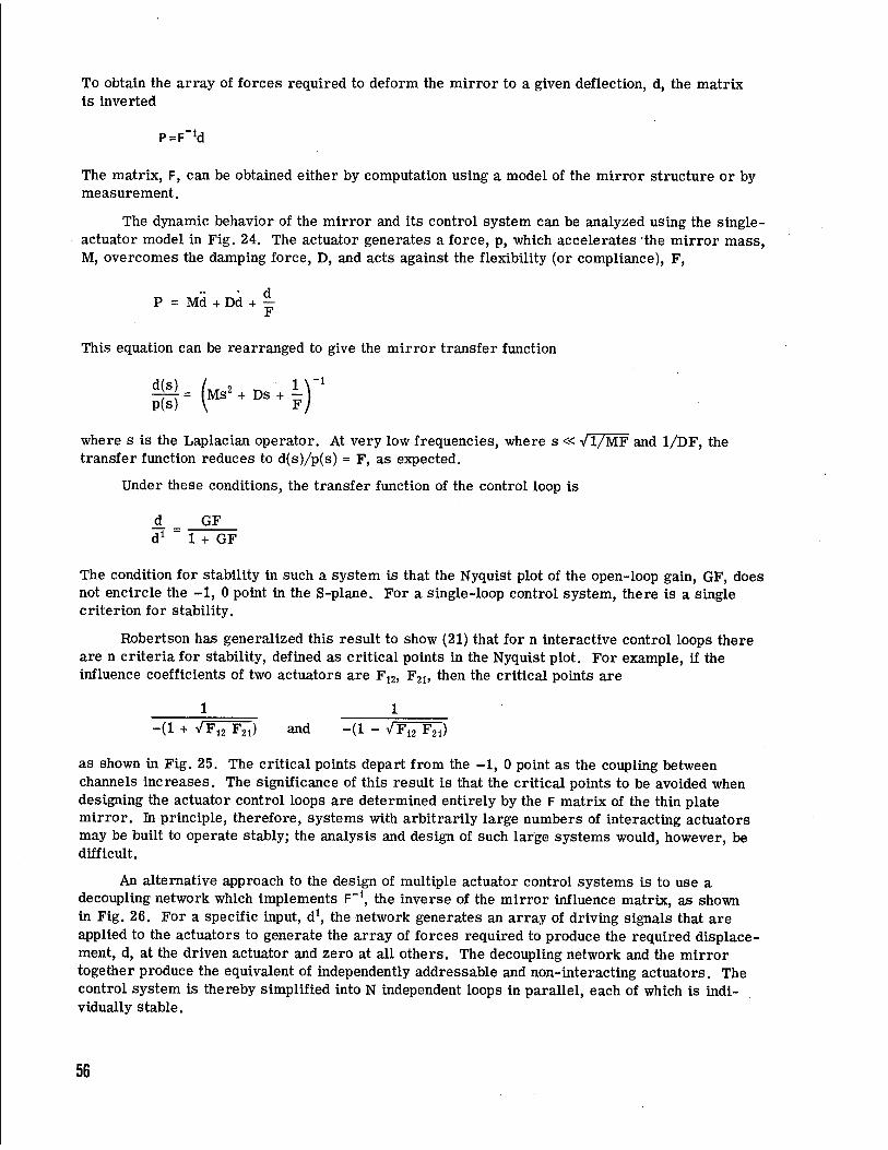
To obtain the array of forces required to deform the mirror to a given deflection, d, the matrix is inverted

P=F~1d

The matrix, F, can be obtained either by computation using a model of the mirror structure or by measurement.

The dynamic behavior of the mirror and its control system can be analyzed using the single - actuator model in Fig. 24. The actuator generates a force, p, which accelerates the mirror mass, M, overcomes the damping force, D, and acts against the flexibility (or compliance), F,

P = Md + Dd + ^- F

This equation can be rearranged to give the mirror transfer function

d(s) P(s)

(Ms2 + Ds + — j

where s is the Laplacian operator. At very low frequencies, where s « Vl/MF and 1/DF, the transfer function reduces to d(s)/p(s) = F, as expected.

Under these conditions, the transfer function of the control loop is

jd_ = GF d1 1 + GF

The condition for stability in such a system is that the Nyquist plot of the open-loop gain, GF, does not encircle the -1, 0 point in the S-plane. For a single-loop control system, there is a single criterion for stability.

Robertson has generalized this result to show (21) that for n interactive control loops there are n criteria for stability, defined as critical points in the Nyquist plot. For example, if the influence coefficients of two actuators are F12, F21, then the critical points are

1 1 -(1 + VF12 F21) and -(1 - VF12 F21)

as shown in Fig. 25. The critical points depart from the -1, 0 point as the coupling between channels increases. The significance of this result is that the critical points to be avoided when designing the actuator control loops are determined entirely by the F matrix of the thin plate mirror. In principle, therefore, systems with arbitrarily large numbers of interacting actuators may be built to operate stably; the analysis and design of such large systems would, however, be difficult.

An alternative approach to the design of multiple actuator control systems is to use a decoupling network which implements F"1, the inverse of the mirror influence matrix, as shown in Fig. 26. For a specific input, d1, the network generates an array of driving signals that are applied to the actuators to generate the array of forces required to produce the required displacement, d, at the driven actuator and zero at all others. The decoupling network and the mirror together produce the equivalent of independently addressable and non-interacting actuators. The control system is thereby simplified into N independent loops in parallel, each of which is individually stable.

56

Actuator G

Force P

Deflection d

77777777777777777777'

Fig. 24 — Single-actuator control model for thin plate mirror

.1-(F12F21)1/2] '°

-1.Ö • ,«

]w

S plane

GF

Fig. 25 — Nyquist plot for two-actuator system. (H. J. Robertson, Ref. 21)

57

Position sensor 1

L) 1 d, Decoupling

network

F"'

Actuators

G

Mirror

F 1 1 1 1

d'N' i

Position sensor N

Fig. 26 — Mirror control system with decoupling network

58

The matrix F"1 is markedly diagonal, i.e., the forces required to produce a given mirror deflection decrease rapidly with distance away from the deflected point. Robertson reports that for a 58-element mirror, the maximum useful array consisted of 19 points arranged as two concentric rings around each deflected point, as shown in Fig. 27. The 19 forces were adjusted to meet three requirements:

1. Sum of forces equals zero 2. Sum of the moments of the forces about the center point equals to zero 3. Force matrix for the complete mirror to be symmetrical about the diagonal.

POSITION ACTUATORS

Of the many possible types of position actuators, the most used are electromechanical (motor-driven screws) and piezoelectric devices. Screw-type position actuators are employed in applications where simplicity and reliability take precedence over high precision, such as in aligning the light-bucket mirrors used for collecting solar energy. For precise mirror control they have given way to force-type actuators, described later.

Several types of piezoelectric devices have been developed for active mirror control; some basic types are shown schematically in Fig. 28. The simple disc or cylinder shown at Fig. 28a may be used singly or in stacks. It is polarized across the thickness and gives a displacement Az = Ed33t, where E is the applied electric field = v/t volts per meter, t is the thickness, and d33

is the piezoelectric coefficient in the direction of polarization (meters per volt). Note that the deflection in this mode is independent of the thickness, up to the maximum (depolarizing) field, a typical value of d33 being 3.7 x 10"10 meter/volt. However, the maximum deflection increases with thickness.

The sensitivity may be increased by stacking plates with alternating polarity as shown in Fig. 28b. The plates are in series mechanically but may be connected in parallel electrically, producing a larger deformation for a given applied voltage. Such stacks tend to be unstable mechanically due to the multiple bonds between layers, and do not necessarily remain parallel when exercised electrically.

In the tubular configuration shown in Fig. 28c, the electrodes are on each side of the wall and the device is polarized radially. The deflection takes place along the length of the tube, L, and is given by Az = Ed31L, where d31 is the piezoelectric coefficient for the direction normal to the polarization. A typical value of d31 is -1.7 x 10"10 meter/volt. While this is lower than d33, the sensitivity of a tube can be improved by reducing the wall thickness (to increase E) and by increasing the length, L. This type of actuator has good structural properties, and is popular for small high-bandwidth active mirrors.

A variant on the tubular configuration is the split cylinder shown in Fig. 28d, which uses three longitudinal slices of piezoelectric material in parallel. The voltages applied to each element can be trimmed to adjust parallelism of the top surface, or to tilt it if required.

In these devices, the properties of the piezoelectric materials are of paramount importance; characteristics of several materials are listed in Table 4. Hysteresis can affect the performance of positioning devices, and tends to be higher in devices with large values of d33. Better overall performance is often obtainable with materials of lower sensitivity. Other factors affecting system design are the loss factor, the coefficient of thermal expansion, and the maximum electric field.

The resonant frequency of actuator devices is normally much higher than the servo bandwidth of large mirrors; it is, however, an important factor in high-bandwidth mirrors and is discussed in a later section.

59

Driving point

(a) Interior Actuator Locations

Mirror edge

Driving point

(b) Edge Actuator Locations

Fig. 27 — Driving force configurations required to obtain displacement at one actuator only in a thin-plate mirror. Numbers indicate relative magnitude of forces. (H. J. Robertson, Ref 21)

60

(a) Disc

(b) Stack

(c) Tube

V

(d) Split tube

^

Fig. 28 — Piezoelectric actuator devices

61

Table 4 — Characteristics of Lead Titanate Zirconate Piezoelectric Materials

Piezoelectric constants d33 10"12 m/V

g33 10-3Vm/N

gi5

Dielectric loss tangent, tan ö

Low field

2kV/cm rms

4kV/cm rms

T Free dielectric constant, K33

T Kii

Curie point deg C

Density (min) 103 kg/m3

Mechanical Q

Elastic constants Y^j 1010N/m3

E Y33

* As defined in MIL-STD- 1376 (SHIPS).

U.S. Navy Type *

I II III

280 380 215

-125 -175 -96

495 595 335

24.4 24.5 24.4

-10.7 -11.2 -10.

38 37.9 29.1

.004 .02 .004

.02 — .007

.04 — .01

1300 1750 1000

1475 1775 1300

>300 >350 >300

7.75 7.6 7.55

500 75 1100

8.2 6.4 8.6

6.7 5.4 7.5

62

A different class of position actuators is based on peristalsis, in which a traveling wave of compression in a hollow cylinder generates axial motion in a closely fitting rod. These devices are characterized by a large total range of travel combined with the capability of making very small individual steps, so that high-resolution positioning is obtainable.

The simplest type of peristaltic device consists of three elements; a device of this type is the Inchworm* shown in Fig. 29. The device consists basically of three coupled PZT cylinders on a metal shaft. The first and third cylinders fit closely on the shaft, while the central cylinder has clearance. The Inchworm is operated by applying a programmed sequence of voltages to the three cylinders, causing the shaft to creep axially in precisely controlled steps. The sequence is started by applying voltage to the first cylinder so that it tightly grips the shaft. A voltage is then applied to the second cylinder to make it stretch by a fixed amount, thereby moving the third cylinder along the shaft. The third cylinder is then clamped, the first cylinder released, and the voltage on the second cylinder reduced to zero.

In this process the piezoelectric structure has "inched" the shaft by a distance exactly equal to the stretch in the central cylinder. The first cylinder is then reclamped and the process repeated.

A plot of displacement versus time is shown in Fig. 30. The control voltage is applied as a staircase of 248 steps at a maximum stepping rate of 220 kHz, causing a total motion of approximately 0.6 micrometer in 1.1 milliseconds. The time required to clamp and unclamp is fixed at 2 milliseconds, so the maximum running speed is about 0.2 mm/sec. The running speed can be varied over a range of about 105, and the minimum resolvable step is stated as 6 nanometers. The maximum load is 22 newtons. Potential problems with this type of device are temperature changes and wear of the piezoelectric elements, which affects the fit on the shaft; the fit can be compensated electronically by applying a bias voltage. Discontinuities may appear in the motion at the clamping intervals, as shown in Fig. 30.

FORCE ACTUATORS

The use of force actuators considerably reduces the effects of backplate deformation; however, they can be used only with stiff faceplate structures. The force is applied through a spring of constant K so that the applied force is equal to Kx, where x is the actuator displacement. The spring constant, K, is made smaller than that of the faceplate, so that a large displacement, x, is required to produce the required faceplate deflection. This is advantageous because the required mirror deflections are generally very small (in the order of micrometers), and the larger actuator motion obtained in this way makes the actuator and the backplate easier to build.

A force actuator designed for use on a stiff primary mirror is shown in Fig. 31. This device uses a motor-driven ball screw to apply the force to the spring; using this approach, electric power is only required to change the applied force, which holds when the power is removed. The force is controllable in increments of 0.1 percent of the maximum of ±445 newtons.

Electromagnetic transducers (similar to a moving coil loudspeaker drive) are also usable as force actuators; they have the advantage of a much higher frequency response than the mechanical screw device, but of course require continuous application of power, which is a drawback in some applications.

Peristaltic devices mentioned previously are also usable as force actuators when combined with a spring.

*Burleigh Instruments Inc., E. Rochester, New York, Patent Pending.

63

Cylinder 2

Cylinder 1 \ Cylinder 3 \ \ / Metal

v//////////^^M(//////////A /haft •*—*-

w////////mmmmm Fig. 29 — Inchworm device, showing the three connected piezoelectric cylinders which are energized in sequence, causing the metal shaft to creep through the structure.

S

c o •ft -t->

I

4.5

3.0

1.5

10 12 14 16 18 20

Time, mS

Fig. 30 — Inchworm displacement versus time. Each step (or ramp) moves the shaft up to 0.7 lira and is followed by a 2 mS period for clamping and unc lamping.

64

Force

Ö35KJ

Spring

-Ball screw

Force

Fig. 31 — Force actuator for a large primary mirror. With this type of actuator, the applied force is not affected by structural deflections and is maintained when the driver power is turned off

65

By using two springs, a weak one on the actuator and a strong one attached to the baseplate, a force actuator can be used with freely supported mirror segments. This method was used in the experimental three-section 56-centimeter mirror shown in Fig. 22. It reduces the effective motion of the actuator in the ratio of the spring constants. The net result is to make the mirror segments stiffly supported from the backplate so that the mirror becomes sensitive to backplate distortion; it does, however, decouple any changes in the actuators themselves.

BENDING MOMENT ACTUATORS

The third basic approach to mirror deformation is to apply bending moments, as described by Scott (46). This technique allows the mirror shape to be adjusted without applying external forces from a backplate.

The basic implementation, shown in Fig. 32, is to attach lever arms at the locations on the deformable mirror where moments are to be applied and then to apply a force between pairs of arms, thereby setting up equal and opposite bending moments. For interior locations on a thin flat plate, the deflection is of the form

where M is value of each moment, d is the separation between moments (much less than the radius of the plate), D is the plate stiffness as previously defined, and K is a parameter dependent on the plate geometry.

Scott has computed the deflection at 217 nodes on a uniform circular plate due to two moments, one at the center and the other located at one of eight different radii, as a standard case. These data may be used to determine the deflection due to bending moments at any point on a new mirror of similar shape by breaking down the moment applied between two locations on the mirror into radial and tangential components, determining the standard deflections, and then adding and scaling them for the new mirror.

The optimum locations for the bending moments are not necessarily the same as those used for force actuators. Scott has found that six moments (three actuator elements acting diametrically between six equally spaced levers) will satisfactorily correct defocus and astigmatism (Zernike polynomial terms 24, 25, and 26) giving an rms error of less than 3 percent of the total deflection. To correct the first 10 Zernike terms to a 1 percent rms level, 24 applied moments are required.

A piezoelectric actuator bonded directly to the faceplate has been used as a bending moment actuator by Berggren and Lenertz (47). The piezoelectric disc was 2.5 centimeters in diameter and 1 centimeter thick, with electrodes on the two flat surfaces. Application of a voltage across the disc results in a thickness change due to the d33 piezoelectric coefficient in the direction of polarization, and also a change in the radius of the disc due to the d31 piezoelectric coefficient. The thickness change has no effect, but the radial change exerts a bending moment on the plate.

Practical thin-plate active mirrors have been made with diameters ranging from 10 centimeters to several meters, covering all three of the main operating regimes shown in Fig. 20. Some representative examples will now be briefly described to illustrate the application of the basic techniques described above.

The first example is a 76-centimeter-diameter mirror with 81 actuators built by Perkin- Elmer for NASA (19). The purpose of this effort was to develop the active figure sensing and control concepts required to obtain diffraction-limited performance of a large telescope mirror in space.

66

The concept is shown schematically in Fig. 33, and a side view of the complete mirror showing the actuators and backplate is shown in Fig. 34. The faceplate is 12-millimeter-thick fused silica figured with a spherical mirror surface. The force actuators apply the controlling forces through springs to 12-millimeter-diameter Invar plugs bonded to the faceplate. The mirror is tied to the 19-millimeter cast aluminum backplate by a kinematic reaction support system, using three supports.

The actuators are driven by dc servomotors and each is capable of exerting up to ±8.9 newtons of force on the mirror. The actuator attachments are stiff axially but have compliance in bending to minimize lateral stresses due to manufacturing tolerances and alignment. The minimum resolvable motion at the mirror was less than 1/250 wavelength at 6328 A (2.5 x 10~9

meter) with a dynamic range of more than ±25 wavelengths. The 76-centimeter mirror had an initial figure error of greater than 0.5 wave rms, which was decreased to less than 0.02 wave rms by the active control system. The mirror was operated with a time constant of 90 seconds, corresponding to a control system cutoff frequency of about 0.002 Hz. The figure sensor used has been described in Section III.

In contrast to the figure-control system with its very long time constant, the next examples of thin plate active mirrors, which were designed for real-time correction of atmospheric turbulence, have time constants of less than a millisecond.

Fig. 35 shows a seven-element experimental active mirror made at Itek (52). The faceplate is 3-millimeter-thick quartz, polished flat. The backplate is 25-millimeter-thick stainless steel whose thermal expansion coefficient closely matches that of the faceplate. The seven discrete position actuators are piezoelectric cylinders that transmit force via flexures, which have a three-millimeter-diameter pad for bonding to the back of the faceplate.

The mirror was assembled from front to back, by first optically contacting the faceplate to an optical flat, bonding on the flexure/actuator assembly, and then finally bonding the actuators to the backplate. After the bonding had cured, the faceplate was separated from the optical flat and then aluminized.

The mirror had a dynamic range of ±3 micrometers for ±1000 volts applied, with a residual error in the flat condition of less than 1/10 wave rms at 6328 A. The useful frequency range extended up to 700 Hz, with the first faceplate resonance at 800 Hz.

The final example of a thin plate mirror is the 37-actuator device made by Hughes (67) shown in Fig. 36. This mirror is made entirely of beryllium and uses piezoelectric position actuators consisting of stacks of discs 19 millimeters long and 6 millimeters in diameter. Each activator can produce 0.56 fim of surface motion for 300 volts of drive.

Influence function profiles of this mirror are shown in Fig. 37. The response of this mirror is of the form exp (-ar1,5), which is termed "sub-Gaussian;" the response is relatively wide, amounting to 23 percent of the adjoining actuators. Toward the edge, the influence functions become skewed. The frequency response is flat up to about 20 kHz, with the first major faceplate resonance at 23 kHz. The authors report that faceplate resonances can be strongly damped by filling the space behind the faceplate with viscous oil; in this way the useful frequency range can be extended to nearly 40 kHz.

The influence function can be narrowed to produce a "super-Gaussian" response of the form exp(-br2-5) by filling the space behind the faceplate with a solid material such as epoxy; this results in some loss in sensitivity. The device then takes on some characteristics of the monolithic mirrors described in the next section, but lack the stability of a homogeneous block.

67

Mirror faceplate

Substrate

-^ ^-

Fig. 32 — Bending moment actuator

PRIMARY MIRROR

MIRROR FIGURE ERROR SENSOR

Fig. 33 — Schematic diagram of thin plate telescope mirror with active figure control

68

Fig. 34 — 76-centimeter deformable mirror assembly, side view showing arrangement of force actuators (H. J. Robertson, Ref. 21)

69

Fig. 35 — Thin-plate active mirror with piezoelectric position actuators

70

41-PIN ELECTRICAL CONNECTOR

ACTUATOR LOCATIONS (3 RINGS) 3.98 DIA

CLEAR APERTURE

Fig. 36 — Beryllium 37-actuator deformable mirror using PZT stack drivers, (a) Side view (b) Faceplate showing 3-ring circular arrangement of actuators, and (c) Photograph of unpolished mirror. (J. E. Pearson and S. Hansen, J. Opt. Soc. Am., 67, 327, 1977)

8 io CENTER OF < NEAREST c£ 0.8 ACTUATOR 3iS am 0.6 UJU N< n . jJ 0.4 <8; |o 0.2

-1.0 -0.8-0.6-0.4-0.2 0 0.2 0.4 0.6 OS 1.0 r = RADIAL DISTANCE, in.

(a)

-0.8 -0.6 -0.4 -0.2 0 0.2 0.4 0.6 0B 1.0 r= RADIAL DISTANCE, in.

Ö 1.0 <

TOWARD EDGE OF MIRROR /"\ •< / \

iz 0.8 =JO

QO 0.6 / \ mm y \ N-l

3Si °-4 <Q I 0.2 O z 0 ■—i -.

-0.8 -0.6 -0.4 -0.2 0 0.2 0.4 0.6 0.8 1.0

r= RADIAL DISTANCE, in.

(b)

-0.8 -0.6-0.4 -02 0 0.2 0.4 0.6 0.8 1.0 r= RADIAL DISTANCE, in.

(c) Id)

Fig. 37 — Influence function profiles of beryllium mirror, (a) Center actuator, (b) First ring actuator, (c) Second ring actuator, and (d) Third (outermost) ring actuator. The interactuator spacing is 14 mm (0.55 in.) (J. E. Pearson and S. Hansen J. Opt. Soc. Am., 67, 327, 1977)

71

In summarizing the characteristics of thin-plate deformable mirrors, two main items stand out:

1. The actuator influence functions are normally wide, extending out to the first or second ring of surrounding actuators so that in a hexagonal array, six to eighteen adjacent actuators are affected. This interaction must be taken into account in the design of the control system.

2. A thin plate mirror is subject to numerous mechanical resonant modes, the frequencies and amplitudes of which depend on the actuator design and damping.

These characteristics are of greater importance in high-bandwidth mirrors than in large mirrors used for figure control. As the operating frequency gets higher, the problem of obtaining stable operation of a multi-channel interacting control system with additional phase shifts due to faceplate resonances becomes severe. For high-bandwidth operation, interaction and resonance problems are greatly reduced in the monolithic active mirrors described next.

MONOLITHIC ACTIVE MIRRORS

The concept involved in monolithic active mirrors is to use for the mirror substrate a homogeneous block of material in which local deformations can be induced and controlled by external means. In effect, the functions of the faceplate, actuators, and backplate are all combined in one monolith.

Devices of this type can be expected to have good" mechanical properties such as stiffness, stability, and shock resistance, making them more tolerant to an operational environment than conventional active devices assembled out of a multiplicity of parts.

The relationship between such devices and conventional active mirrors echoes in many respects the relationship between transistors and vacuum tubes.

At the present time, only one such device, the monolithic piezoelectric mirror (MPM), is known. This device was developed at Itek by Feinlieb, Lipson, and Cone (38) and has proved to be admirably suited for correction of atmospheric wavefront distortion at visible wavelengths. The basic construction of an MPM is shown in Fig. 38; it uses a circular slab of lead zirconate titanate (PZT) piezoelectric ceramic typically 5 to 10 centimeters in diameter and 1.2 to 2.5 centimeters thick. An array of electrodes is located at the top surface to each of which is applied a control voltage, using the electrode at the base of the slab as a common reference. A thin glass bonded to the top surface is optically polished and aluminized to form the reflecting surface.

The MPM has the following characteristics:

1. When voltages are applied to the electrodes, the piezoelectric deformation all occurs close to the top surface and no deformation occurs at the base.

2. The induced deformations are localized in the vicinity of the activated electrode.

3. The coupling between neighboring electrodes can be adjusted from zero of at least 20 percent by varying the geometry of the electrodes.

4. There is no measurable bending of the block when voltages are applied to the electrodes.

Hudgin and Lipson (45) have analyzed the MPM and find that the surface deformation for a plate of infinite thickness may be approximately expressed as

Ms(Y) = db + ^+(i + ff)du]v°cos/,y

72

ALUMINIZED GLASS MIRROR

ADDRESSING ELECTRODES

PIEZOELECTRIC CERAMIC

COMMON ELECTRODE

ELECTRICAL ADDRESSING LEADS

Fig. 38 — Construction of monolithic piezoelectric mirror (MPM)

73

where JUX(Y) is the deformation measured perpendicular to the surface x = 0 at point Y, V0 cos jSy is an applied sinusoidal voltage at the surface, du, d12, d26 are the piezoelectric coefficients, and a is the Poisson ratio. For a plate of finite thickness, t, the solution is obtained numerically. The surface sensitivity (meters per volt) is constant for values of the parameter ßt greater than 3, where ß is the wave number, 2TT/X, of a sinusoidally varying surface voltage. The condition for zero dispersion is therefore that the PZT thickness should be greater than half the longest spatial wavelength to be impressed on the surface.

The sensitivity of practical devices is in the range of 0.25 to 0.5 micrometer surface deflection per kilovolt, depending on the type of PZT material. The maximum interelectrode voltage is limited by the depolarization field, which is typically 1.5 kV/mm.

Some control can be obtained over the sensitivity and the shape of the influence function by varying the electrode configuration and the glass thickness.

A typical MPM response function is shown in Fig. 39 and is of the form [1 - (r/L)2]2, where r is the radius from the center of an actuator and L is the actuator spacing. The shape remains constant over the whole surface.

The frequency response of MPM devices is extremely good, being limited primarily by the natural modes of the PZT block, which because of its large thickness-to-diameter ratio, occur at high frequencies. Typical devices have a flat response to over 10 kHz and have been operated at discrete frequencies as high as 60 kHz, although such frequencies can excite resonant modes.

A typical MPM is shown in Fig. 40 and interferograms depicting the surface deformations achievable are shown in Fig. 41.

Because of the small interaction between actuators, the compensating networks usually required with thin plate mirrors are not necessary with MPM's, resulting in some simplification of hardware. However, MPM actuator sensitivity is lower than with discrete PZT actuators, requiring higher driving voltages.

Monolithic piezoelectric mirrors have been used in the Real-Time Atmospheric Compensa- tion System described by Hardy et al. (69). Experimental MPM's have been built with 300 active elements within a 75-millimeter diameter.

MEMBRANE MIRRORS

A membrane is distinguished from a thin plate by having no inherent stiffness so that tension must be applied to maintain flatness; relatively small forces are required to obtain the deflections necessary for optical wavefront correction. The simplest type of membrane mirror is the "varifocal" mirror described in Section n, in which a reflectively coated membrane is acoustically coupled to a piston (in practice a loudspeaker) producing changes in the radii of curvature and therefore the focal length, of the mirror.

The use of membranes as high bandwidth, high-order active mirrors has been pioneered by Yellin (55) and Grosso et al. (74) at Perkin-Elmer. A schematic diagram of an electrostatically driven membrane mirror is shown in Fig. 42. The metal membrane is typically 0.5 to 1.0 micrometer thick and is positioned between a transparent electrode carrying a bias voltage VB

and an array of electrodes, to each of which is applied the bias voltage plus a signal voltage Vs. The membrane is at ground potential, and experiences no net force so long as Vs = 0. When a signal voltage is applied to one actuator, a deflection is produced; centered around that actuator. The membrane is operated at low air pressure (2 torr) to obtain a favorable compromise between sensitivity (which is maximized in vacuum) and membrane resonant frequency (which is at a minimum in vacuum). The incident light beam passes through the sealing window and the transparent electrode before being reflected off the membrane.

74

-0.4 -0.2 0 0.2 0.4

Distance From Actuator Center, centimeters

Fig. 39 — MPM response function. Interactuator spacing is 3.8 mm

75

Fig. 40 — Monolithic piezoelectric mirror

76

<A)

(B)

Fig. 41 — Interferograms showing controlled surface deformation of a monolithic piezoelectric mirror. Each fringe represents one wavelength (0.633 ßm) of wavefront deformation

77

j- -PUPIL REGION -J

rrn TUT i X. V0±AVj /

TRANSPARENT ELECTRODE

ACTUATORS

BOUNDARY CONTROL PADS

(a) Membrane actuator drive schematic

O-RINGS MEMBRANE

SPRING \\

WINDOW PAD ARRAY

MYLAR SPACERS

MEMBRANE MOUNT

.CONNECTOR

30 GAUGE TEFLON INSULATED COPPER WIRE

(b) Membrane mirror assembly

Fig. 42 — Membrane mirror with electrostatic drive. (R. P. Grosso and M Yellin, J. Opt. Soc. Am., 67, 1977)

78

The equation of motion of an ideal membrane with no viscous damping, with an external force, F, applied at a location r from the center is

32Z _ T y2 F(r, t) Ip" a a

where Z is the displacement, t is the time, T is the tension/length, a is the mass/area, and V2 is the Laplacian operator.

The steady state deflection is given by

v'z - - Spl

Thus, to produce a given deflection, Z, the force applied to the membrane must be the Laplacian of the required deflection.

The wavefront sensors used for active optics produce as outputs either a set of values representing the wavefront map or a set of phase differences from which the wavefront can be reconstructed. With either type of outputs, some computation is required to obtain the Laplacian signal required to drive a membrane mirror. This computation is minimized with the Hartmann and Shearing interferometer sensors (described in Section in), which produce sets of wavefront differences; the operation required is then to determine the local divergence of the measured wavefront.

When using electrostatic actuators, the steady-state deflection at radius r < s is given by Grosso and Yellin (74) as

Z(r) = e0S^ 4T 4 " *fe

(s2 - r2)

where e0 = 8.8 x 10"12 farad/meter S = actuator radius

£p = spacing of membrane to actuator pads Vp = voltage on actuator pad = Vg + A Vg = voltage on bias electrode ig = spacing of membrane to bias electrode.

The peak deflection when r = 0 and AV = 0.5Vg is

Zmax * fä|r (1.25V*B)

In the typical case quoted by the authors, S = 1.25 x 10"3 meter, i = 80 x 10"6 meter, T = 175 N/m, and Vg = 200 volts, giving a peak deflection for each actuator of Zmax = 0.15 x 10"6 meter. The optical path length correction produced by the mirror deflection is twice this value. Because of the broad influence function of the membrane mirror, which effectively integrates the local deflections at each actuator, the total deflection produced when voltage is applied to many actuators is quite large.

The resonant frequency of the membrane is an important parameter in system design. The lowest resonant frequency (in vacuum) is given by

79

1/2

where D = membrane diameter.

The resonant frequency can be raised by introducing air into the cavity, to give

Von - V. (l ♦ C4)

where P is the pressure (torr) and C0 is a proportionality constant.

Air damping of the membrane is necessary to control the transient response; it is implemented by placing an annulus outside of the actuator array with a narrow gap between it and the membrane.

The fundamental resonance of a 50-millimeter-diameter membrane mirror using a 1.4- micrometer titanium membrane is quoted as 3.8 kHz, in vacuum, which is raised to 7 to 8 kHz with air damping.

ACTIVE MIRROR DATA SUMMARY

Physical characteristics and performance data on all high-bandwidth active mirrors described in the open literature to date are listed chronologically in Table 5.

80

"S CU a u >

I K

o o o CM -H

o o o

O t- o

o O o o o 00 -rH CO o o o -H ■« ■41 CO »* CO

es 0) o

•S1 a £

o ■H

C to <y c N

* co M u tu

Its w <

s a

CM

A

=3

o

° a 8"° J3 'S

en

W CM

O CO

o -"-> o o ■*

t!i

§=3

o CM V

OS GO a o -o

in

•y CÜ

IS

«I Is

J3

of 0) s

O w

.«? o

s

.?> o ft 3 ft 3 ft 3

8 •f-l

a

S 2 ft 3

43

o & .a a ft s ft B

<» ■ M ft

ll ft B O Gj

Ä I» H

a-

■a | ft ^

£

o N id

CD 0) -2 ft B

c 1 it 01 01 ft CO

eg ä Ü

ft B

a) e? w co

<U

I EH

u

f * 'S 0)

la 1 .5 t- a

a CU a 1 "3

a § <U X I <u

t- 43

I g «U *<

ä 3 CO

I I cu 8

0) g

cu jij

0) g

CO

u cd

a g 71 *

a a

a I

tl

fH

o o S 2 S a 5 B S a

I -a c B oa

•r-t

ft

a o CO

ft B a C «>

1 t3 H ft

Is EH ft

^ !2 c

■a 7S 0) 4_) -t->

10 CD

0>

* ll a c •rH S3

't. O 0 «> 05 [^ U PH

■&

o CO

S3 ft

"3> ^_ to C3S *-^ »-I

CO t-

"3 05 r*

■u 0) a O CO

o

13 CD 12 ft ««

c» ^ -a

- ® C CO

3 §

c-

C£7 CM CO

C- ^^ t- I- o> c- rH

l CO cu

0)

0)

1 1 g

CO a s o cu cp CO u K ft X s #

81

V. SYSTEM CONSIDERATIONS

After reviewing the various active optics devices and techniques available for wavefront measurement and correction, we now consider how these components are integrated into a functioning system and how that system's performance is optimized.

Some aspects of system design have already been touched on; many of these considerations are familiar ones common to most servo systems, such as dynamic range, residual error, bandwidth, and stability. Consequently, we will consider in this section only those design aspects that are unique to active optical systems. Such systems involve both the spatial and the temporal domains. Spatial considerations involve the number of degrees of freedom (i.e., independent actuators) on a mirror and the spatial resolution of the wavefront sensor. Temporal considerations involve the photon flux and integration time, which determine the signal-to-noise ratio, delays around the servo loop, and the need for prediction. Other factors include the widely changing environmental conditions that are often encountered, especially with atmospheric compensation systems, and that may require adaptive control.

To provide a framework for the following discussion, two system models will be used. The first, shown in Fig. 43, is that of a received wavefront system, typified as an atmospheric compensation system. With minor modifications it will also serve for figure sensing and phase conjugation systems. The second system model is an outgoing wave multidither system, shown in Fig. 45.

Such systems are characterized by the parameters of their key subsystems such as the wavefront sensor and wavefront corrector. System optimization involves consideration of the main sources of error and balancing them to achieve a given goal such as maximum performance or minimum cost.

FIRST SYSTEM MODEL

The purpose of this system is to minimize the residual wavefront distortion, E, in Fig. 43 in order to obtain a nearly diffraction-limited image of the reference source. The incoming wavefront to be measured and corrected is a function of space and time, (p(Xi, t). The photon flux density associated with this wavefront is B photons-m-2-sec"1, and the receiving aperture area is A m2. The wavefront passes through the wavefront corrector, containing Nc individual actuators, which subtracts the estimated correction $(X|, t) from the incoming wavefront to form the corrected wavefront with residual error E. The spatial error associated with this process is termed 'fitting error" and is discussed in a later section. The wavefront sensor then spatially samples the corrected wavefront with a number of subapertures Ns, which is usually but not necessarily the same as Nc. A parallel array of detectors is required for this purpose.

In each subaperture an estimate of the residual wavefront slope A$(Xit) is made using a photoelectron integration time of T seconds. The number of photoelectrons counted per subaperture is

82

Reference source

output

Wavefront disturbance 4> (xi, t)

Wavefront corrector

Nc actuators

Wavefront sensor

NS subapertures

E

«?ps 4, t)

Wavefront predictor

Wavefront reconstructor,

?(Xi t)

A<P (Xi, t)

Fig. 43 — First system model—received wavefront compensation

83

M = Barnq

where 77 = optical efficiency of system from entrance aperture to photosensor q = photosensor quantum efficiency a = A/Ns

The signal-to-noise ratio of the residual slope estimates depends on M and on several other factors that are discussed in the section on photon error. The noisy residual slope measurements are reconstructed into (less) noisy residual wavefront estimates <jt>(Xit); up to this point the average age of each measurement is 1/2 T.

The final stage in the loop is the wavefront predictor whose function is to smooth the measured data and convert it into signals representing the next predicted wavefront 0(Xi, t) that will be applied to the wavefront corrector. In its simplest form, the predictor is a high-gain integrator, as used in the RTAC system (69), which may be characterized by a smoothing time constant, ts. More complex methods of prediction for use in atmospheric compensation systems have been investigated by Hudgin (72) and will be briefly described later.

The main sources of error in an active optical system such as that shown in Fig. 43 are:

1. Wavefront fitting error, CTF

2. Wavefront measurement errors, aM

3. Prediction or time delay errors, Op.

These error sources are considered in the following sections. In addition, there are numerous miscellaneous sources of wavefront error due to hardware tolerances and misalignments that can be lumped together as a quasi-fixed error, aH, usually small.

The total system wavefront error may then be expressed as

°T = °F + °M + °P + °H

WAVEFRONT FITTING ERROR

Wavefront fitting error is caused by the necessarily finite number of degrees of freedom in a wavefront corrector, which limit the precision with which a given phase function can be corrected. In the case of a mirror figure control system, the required phase function <p(X, t) is generally of low order and is often decomposed into the classical optical aberrations such as tilt, deforms, astigmatism, and coma.

Hudgin (73) has shown that if the wavefront corrector response function of the j-th actuator for unit signal is Rj(S), then the minimum mean square fitting error is

N emin = eo ~ ZJ BjCJk BR

where

Bi = i foWRjW

84

CjK = { JdXj(X)RK(X)

e„ = j Jdx 02(X)

A = aperture area

N = number of actuators

The correction to be applied at each actuator is then

N

K=l ]K K

In the case of time-varying wavefronts encountered in atmospheric compensation, a statistical approach must be used. The ensemble average fitting error is then

N <(emin^> = <e„)> - 2 Cj£ BjBK

which gives

<^emin> = äi* Jdx dy D(x " y) + W 2 CJK JdX dy Rj(x)RK(y)°(x " y)

where D(x - y) is the wavefront structure function. For atmospheric turbulence, the function D(x - y) = Clx - y|5/3 corresponding to a Kolmogorov spectrum is normally used.

Hudgin has calculated the residual fitting error <emin^ as a function of the ratio L/r0, where L is the actuator spacing and r0 is the atmospheric coherence length defined by Fried (13). For the response functions shown in Fig. 44, the fitting error is of the form

°F=<fmln>= «(LA,,)5'3

where a is a constant depending on the shape of the response function. Values of a for various response functions are shown in Fig. 44.

WAVEFRONT MEASUREMENT ERRORS

There are two unavoidable errors associated with measurement of a wavefront: the sampling error and the photon flux error. Additional errors may be due to optical system tolerances and misalignment or to electrical noise in the wavefront measuring system.

The sampling error is exactly analogous to the fitting error previously discussed in relation to wavefront correctors. If the subaperture size in the wavefront sensor is the same as the actuator spacing in the corrector (and there appears to be no reason for having it otherwise), then the error need only be accounted for once. If the subapertures and actuator spacings are different, then the fitting error may be found by using an effective spacing

85

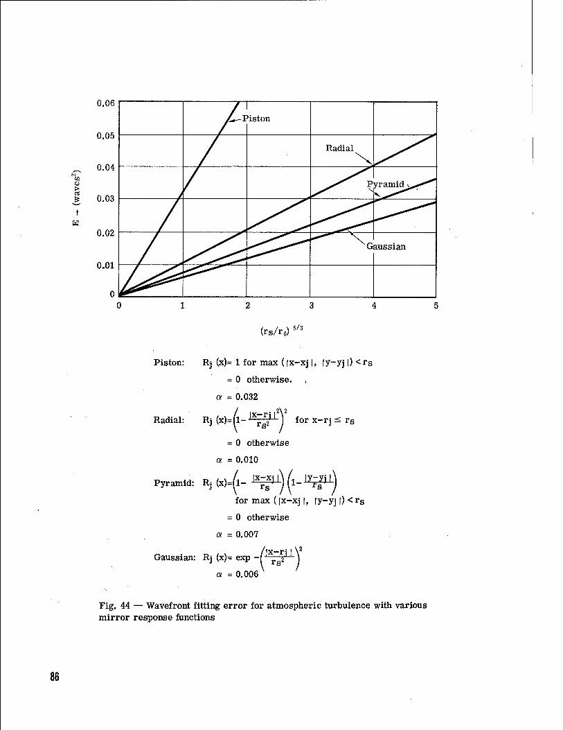
CD

w

0.06

0.05

0.04

0.03

0.02

0-01

/ 1 L*- Piston

Radial

_J>tr Pyramid v-*»"^

Gaussian

(rsAo 5/3

Piston: Rj (x)= 1 for max (|x-xj |, |y-yj |) <rs

= 0 otherwise. ,

a = 0.032

x-rj^2

Radial: Rj (x)=fl- ' 2'' ) for x-rj < rs

= 0 otherwise

a = 0.010

Pyramid: Rj (x)=(l- ^ (l- ^

for max (|x-xj |, |y-yj |) < rs

= 0 otherwise

a = 0.007

/|x—ri ' ^2

Gaussian: Rj (x)= exp -{' r^2

a = 0.006 rs"

Fig. 44 — Wavefront fitting error for atmospheric turbulence with various mirror response functions

86

Leff aV!

where Ls and Lc are the sensor aperture and corrector (actuator) spacings. A further conse- quence of using a measuring aperture of finite size is that residual wavefront curvature within one subaperture reduces the modulation of the detected signal and thereby reduces the signal-to-noise ratio..

If the reference light source used by the wavefront sensor produced a nearly infinite photoelectron count during the allowable measurement integration time, then the photon flux error would be vanishingly small, and the system error would be dominated by the fitting errors just described. This condition is often approached in figure-sensing systems where the allowable integration time is very long, often tens or hundreds of seconds.

At the other extreme are atmospheric wavefront compensation systems, where the photoelectron count from a reference source such as a star within the atmospheric decay time of about 10 milliseconds may be less than 100. In such cases there is a tradeoff between photon error, which decreases with longer integration time, and the wavefront prediction error, which increases with integration time. The optimum is reached when these two errors are equal. In a system where the photon flux and/or the wavefront dynamics change over a period of time, adaptive control over the integration time will be necessary to optimize performance.

SHEARING INTERFEROMETER

For an ac lateral shearing interferometer in which the detected signal is sine-wave modulated, the minimum error in measurement of tilt over one subaperture due to photon noise using sine/ cosine weighting functions in the phase detector is given by

°2 = M7 ^waves'

where M = total photoelectrons used in measurement y = fringe visibility L = subaperture spacing S = shear distance.

The fringe visibility is determined mainly by the angular size of the reference source (51). For a given photon flux density B, the photoelectron count M is proportional to the subaperture area, which is proportional to L2. Thus, for optically efficient systems in which the subapertures completely cover the wavefront, the error in the measurement of local tilt is independent of the size of the subapertures.

When the measured local tilts of the wavefront are combined to form the actual wavefront using the reconstructor shown in Fig. 13, the overall photon error is reduced by a factor of about 0.75 and is only weakly dependent on the number of subapertures (71).

HARTMANN SENSOR

In the Hartmann sensor, described in Section HI, the wavefront to be measured is divided up into many subapertures, the light from each subaperture being brought to a separate focus to produce multiple images of the reference source. The position of the center of intensity of each image is tracked by means of a detector in order to measure the average wavefront tilt in each subaperture.

87

The performance of a Hartmann sensor depends greatly on the size and shape of the reference source image as well as on the type of detector used. For an optimum detector, i.e., one matched to the intensity distribution of the reference source, the tilt measurement error over one subaperture is

, 3 °opt 4ir2M (-W waves2

where a = angular subtense of reference source (assumed circular) X = mean wavelength.

For the more practical case of a quadrant detector, the error variance is over three times greater

2 _ J_ °quad - 4N

L La l1+T-

La\2

waves2

PREDICTION OR TIME DELAY ERRORS

Time delay errors become important in real-time correction systems when changes in the wavefront may occur within a few milliseconds. In received wave systems, the main time delays are the wavefront sensor integration time r, the smoothing time constant ts, and the corrector time delay tc, which includes any computation time required. Usually ts is the dominant time constant in the loop, determining the servo system response. In transmitted wave systems where the corrected wavefront has to make a round trip to the target before being measured, the transit time may add significantly to the total delay. In figure control systems, ts may be tens of seconds and is determined entirely by servo system and noise requirements.

t

For atmospheric compensation systems, ts determines the prediction error according to the relation

Oj = Cf tff»

where Ct is the time-structure function of the atmospheric propagation path. Normally the smoothing time ts will be adjusted to equalize om and op.

The prediction error may be reduced by using knowledge of the wavefront statistics to utilize samples selected from previously measured wavefronts. Hudgin (72) finds that for temporal averaging alone, the use of two previously measured wavefronts with appropriate weighting is nearly optimal and that going back further in time is unproductive. However, the use of combined • space-time estimation gives a dramatic improvement; the use of 10 phase points, distributed in space and time over 10 previously measured wavefronts, reduces the prediction error by a factor of about 4 over a simple integrator, providing that the wavefront sensor phton error is less than the system time delay error. Implementation of such a system requires a considerable computation capability.

SECOND SYSTEM MODEL

An entirely different system application is represented by the second model (Fig. 45). The objective here is to maximize the intensity of a laser beam on a target, after traveling through a turbulent atmosphere. The laser beam is split into N elements, each of which is tagged by a dither frequency o)n to produce a time-varying phase ip sin wnt, where ip is the amplitude of the modulation. The beam passes through the wavefront corrector, which impresses on it by means of independent piston actuators, the phase correction required to compensate for the wavefront disturbance encountered by that section of the beam in its journey to the target.

88

Target

Wavefront disturbance <Mt)

Wavefront corrector

N elements

Tagging array

N elements

Detector

LP filter

Sync detector

Laser source

Dither amplitude iji

© wn

Fig. 45 — Second system model—outgoing wave multidither system

89

The total field on the target may be expressed as (65)

N ET(t) = X AnE0 exp i<fo(t)

n=l

where E0 = magnitude of field per subaperture at source Ajj = subaperture weighting and fitting factor

4>n(t) = time-varying phase of the n-th wave = fti(t) + *P sin wnt-

The total intensity within the diffraction-limited area Ad on the target is

N N N

S S n=l n=l m=l

IT = |ETI2 = E2 1 £ An + £ £ exp i[fc,(t) - tf>m(t)]

I This expression may be expanded to give

Eg N N N £ An + J?(0) 2 £ cos (ft, - j3m) n=l n=l m=l

N N - 4J0(!/))J1(!/)) YJ X sin (ßn - ßm) sin wn* + higher order terms

n=l m=l

Im + Ij) + higher order terms

The Im term is the mean intensity that is to be maximized.

The light reflected from a small glint (whose area Ag is less than that of A<j) also contains the dither term Irj in which the phase errors (ft, - ßm) have been converted into amplitude modulation at the dither frequencies wn. These signals are picked up by the detector and comprise the means of maximizing the intensity on target. The received signal is actually maximized with respect to a reference phase ft», which is the mean of the remaining (N - 1) channels. For small phase errors

N

1=1 l=c

The intensity at the target may then be expressed as

Irj. - E0

N 2 An + 4(m ~ 4J0WJW) (N - 1 + Hn)1/2 sin (ft, - ft.) Sin «nt n=l

where (ft, - ft.) is the phase error in channel n and H and Hn are convergence parameters defined as

90

N N Hn = 2 £ cos On " 0m)

n=l m=l n^m

Before convergence, the phases are random and Hn is small; at convergence, ßn = ßm and Hn = N2 - N

N N H = V V cos (ßn - ßm) = N2 at convergence.

n=l m=l

The detected signals at frequency wn are filtered and synchronously detected to yield the servo control signal, which is the coefficient of sin wnt in the above expression. The loop gain, which is proportional to this signal, is initially small before convergence, reaches a maximum during convergence, and then drops to near zero when /3n = ßc. The on-axis irradiance at convergence for equal subaperture weighting and no noise is

Ip = E2, N + (N2 - N)J?(0)

This expression shows that on-target power is lost as the dither amplitude is increased.

The signal-to-noise ratio is of the form

S Ag N0 Ad

AmJ^) N (ftx " ßc)2

where BT= effective photoelectron count per servo integration time. For a constant transmitted power and constant beam size, the signal-to-noise ratio varies inversely as the square of the number of elements. However, if the element size remains fixed, the signal-to-noise ratio then varies inversely as N, i.e., as the aperture area. For example, in a transmitted wave system if the number of elements (of constant size) is increased, then the diffraction-limited area A^ is inversely proportional to N, so that for constant transmitted power S/N0 & 1/N. Similarly in a received wavefront system where the power density in the collecting aperture is constant, the photoelectron count becomes proportional to N, resulting again in S/N0 «= 1/N.

To optimize signal-to-noise ratio, the dither modulation should maximize J^ij)). However, as shown by the previous expression for Ip, the dither itself produces a loss in intensity on target. Determination of the optimum dither modulation is a complex system tradeoff, which depends on additional factors such as laser or speckle noise.

The effect of speckle-induced modulation of the received signal due to taget motion has been investigated by Kokorowski et al. (72). Random intensity modulation falling within the detection bandwidth may compete with the desired correction signal and thus impair the convergence process. Computer simulations showed that speckle modulation may have two effects: (1) a reduction in the mean convergence level and (2) a random oscillation of intensity. These effects are negligible if the power in the demodulated dither signal is more than twice that of the signal due to speckle. However, if the speckle signal will predominate and prevent the multi-dither system from converging. Experimental measurements showed that these effects could be minimized by optimizing the servo bandwidth.

91

VI. APPLICATIONS

Within the past decade several experimental active optics systems have been built and tested; the results have been generally successful and confirm that active wavefront control indeed brings a new dimension into the design of high-performance optical systems.

In this section, the configuration and performance of four systems representing the most important current approaches to high-bandwidth wavefront compensation reported in the literature will be briefly described: they are:

• Phase conjugate COAT • Multi-dither COAT • RTAC • Image sharpening.

The first two are laser outgoing-wave systems designed to maximize the energy on a target, while the last two are received-wave systems designed to maximize image resolution.

PHASE CONJUGATE COAT

Experimental results of an infrared phase conjugate COAT system have been reported by Hayes et.al. (63) of Rockwell International. The coherent source was 40-watt C02 laser feeding six or seven subapertures each 25 millimeters in diameter. A block diagram of this system is shown in Fig. 4c. The phase shifters employed were germanium Bragg cells operating at an acoustic frequency of 18 MHz. Each channel employed a PbSnTe infrared heterodyne detector using a common reference beam frequency-shifted by a further Bragg cell operating at 15.75 MHz, to produce an electrical output at 4.5 MHz (double pass). The response time of the system is composed of the optical transit time form the path disturbance to the measuring system and return plus about 10 microseconds processing time.

Target glints were simulated with a 1-centimeter-diameter gold-coated corner reflector. The energy distribution in the vicinity of the target was measured by scanning a HgCdTe detector across the beam.

Tests were made at 1-, 6-, and 9.5-kilometer ranges. Using six beam elements as a close- packed linear array 0.175 meter across, little atmospheric degradation was encountered at 1-kilometer range, the system giving essentially diffraction-limited performance. At 6 kilometers range with six elements spaced over a 0.5-meter aperture, the uncompensated beamwidth with mild turbulence was 0.152 meter. With the loop closed, the beam width was reduced to its diffraction-limited size of 0.125 meter. At 9.5 kilometers range, the signal-to-noise ratio was insufficient to obtain full operation.

The response time at short ranges consisted of a hunting time of 20 to 100 microseconds, followed by convergence in the next 20 to 30 microseconds. The convergence time corresponds to two loop iterations. At low signal-to-noise ratios the convergence time stretched to 2 seconds. Once converged, the bandwidth of the system was 2 to 4 kHz.

92

The authors report that the phase conjugate system consistently locked on to the brightest of two glints even when the difference in reflectivity was only 1 dB. Beam pointing or offset was accomplished by introducing a linear phase bias across the Bragg cell array, although the angular deflection is limited in this case to the beam spread of a single subaperture.

The system also had the capability of time-shared operation, switching alternately between a glint point and a designated aim point. Tracking of a moving target, using the phase shift array only, was also demonstrated.

MULTI-DITHER COAT

A description of the design and performance of an 18-channel multi-dither system built at Hughes Research Laboratories has been given by Pearson et al. (59) and experimental results have been reported by Pearson (60). A block diagram of this system, which operated at the visible wavelength of 488 nanometers, is shown in Fig. 46. The optical power source was 0.5-watt argon ion laser; two separate piston-type phase shifters were employed to implement the tagging and error correction functions. Separate galvanometer-driven mirrors were used to provide offset pointing of the entire beam. The 18 channels were arranged in two concentric rings of six and twelve elements, with a transmitted beam outer diameter of 14.8 millimeters. Dither frequencies were in the range 8 to 32 kHz with a spacing of 1.4 kHz. The phase corrector had a range of over ± 4 wavelengths at 488 nanometers, while the dither mirror provided ± 20 degrees of phase modulation. The receiver consisted of a 20-centimeter-diameter parabolic mirror that focused the radiation reflected from the target onto a single photomulitplier tube. The nominal servo bandwidth of the system was 500 Hz, with a convergence time of 1.5 to 3 milliseconds.

The experiments reported by Pearson (60) were conducted on a horizontal propagation renge about 100 meters in length across a rooftop. Target glints were simulated by 3-millimeter-diameter retroreflectors, which were unresolved by the transmitted beam. The power received by each glint was directly measured by a detector located behind the retroreflector.

Using the power received by a single glint under condition of low «turbulence with the COAT system on as a reference (=1.0), the relative glint power with strong turbulence was 0.15 with the COAT system off and 0.44 with the COAT system on, an increase of 2.9 times in intensity. Cor- responding beam width profiles are shown in Fig. 47, showing an improvement in beam width by a factor of about 5 with the COAT system on. Tracking performance of the system was verified by moving a strong glint near a weak fixed glint; satisfactory operation was observed at the highest available rate of 14 mrad/sec. Experimental observations of the system with two glints showed that if the glint intensities differ by 2 to 3 dB, the system converges on the brighter glint and ignores the weaker one. If the intensities are closer than this, the system may jump from one to the other in time but does not instantaneously share power between them.

The experiments reported were conducted at visible wavelengths as a matter of convenience; Pearson (60) shows how these results are capable of being extrapolated to other wavelengths of interest such as 3.8 micrometers or 10.6 micrometers.

The initial experimental work with multi-dither systems was made with piston-type actuators that provide uniform phase displacements over discrete subapertures. Continuously deformable mirrors have several advantages including smoother fitting of wavefronts, the need for fewer actuators, and the capability of cooling the faceplate for high-energy applications. However, the actuator influence functions of deformable mirrors overlap and produce appreciable response in adjacent channels, causing cross-coupling between the servo loops. Some cross-coupling exists even with piston actuators due to the fact that each channel influences the phase of the common reference, but the coupling due to deformable mirror influence functions has been found by O'Meara

93

BEAM DIVIDER T=*

J TAGGER AND PHASE SHIFTER

ARRAY

llll

18 ELEMENT PHASOR MATRIX OUTPUT ARRAY

MICRO SLEWING — MIRRORS

_, OUTPUT TELESCOPE

TARGET

SERVO ELECTRONICS

ARRAY

SIGNAL CONDITIONING

RECEIVER t-

Fig. 46 — Multidither COAT system block diagram. (J. E. Pearson et al., Appl. Opt, 15, 612, 1976)

/V' f** ****J%»^„JI(>(^I

^%li«»Wili|„|,n i

-—I h*—FWHM=0.52

Coat off Coat on

Fig. 47 — Multidither COAT system beam width profiles in high turbulence. (J. E. Pearson, Appl. Opt., 15, 626, 1976)

94

(66) and Pearson and Hansen (67) to be much more severe. The major problem with a hill-climbing servo is that some channels or blocks of channels may lock up on a subsidiary peak that is displaced by a mulitple of 2TT radians from the mean phase of the corrector, thereby causing a significant loss of intensity.

REAL-TIME ATMOSPHERIC COMPENSATION (RTAC)

The purpose of the RTAC system (37) is to improve the angular resolution obtainable with telescopic imaging systems when viewing distant objects through a turbulent atmospheric path. One of its major applications is in ground-based astronomy, where compensation of atmospheric turbulence would allow a large improvement in the resolving power of existing telescopes.

The RTAC system was initially developed in 1973 at Itek and an improved version was described by Hardy et al. in 1977 (69). A block diagram is shown in Fig. 48. The beam from the telescope is collimated by lens LI to form a beam 2.5 centimeters in diameter, which is directed to the wavefront corrector, a monolithic piezoelectric mirror (MPM) with 21 independently addressable elements. The MPM (described in Section IV) is placed near an image plane of the entrance aperture of the telescope so that the incoming wavefront is mapped at a reduced scale onto the MPM. After reflection from the correction device, the beam is amplitude divided into two parts by the beam splitter B, part going to form the corrected image and part going to the wavefront sensor, which is an ac radial grating interferometer similar to that described in Section IH. The wavefront sensor employs two 16-element phbtomultiplier arrays that bear a one-to-one relationship to the spaces between the 21 elements of the MPM wavefront corrector, one array measuring the optical path differences in the x-direction and the other those in the y-direction, as shown in Fig. 49. The 32 optical path difference measurements are then processed in a parallel analog computer similar to that shown in Fig. 14 to produce a parallel set of 21 spatially smoothed residual error signals, which are then temporally smoothed and applied to the amplifiers that drive the elements of the MPM. The RTAC operates as a closed-loop feedback system with 21 independent parallel channels. In addition, correction for overall wavefront tilt is made by tilting the entire MPM in two dimensions by means of piezoelectric actuators. The optical assembly of the RTAC is shown in Fig. 50 and the complete system is shown in Fig. 51.

RTAC test data were obtained using a low-power He-Ne laser as a reference source both in the laboratory using simulated turbulence and over an outdoor horizontal propagation range. Results of the laboratory tests are shown in Fig. 52; the wavefront error at the output of the RTAC was measured by making shearing interferograms, which were scanned and reduced to obtain wave-- front maps in which the contour spacing is 0.05 wave at 6328 Ä. The corresponding point spread functions (PSF's) were computed from these measured data and are shown as three-dimensional intensity plots. The residual distortion in the RTAC alone was 0.04 wave rms, 0.21 wave peak to peak as shown in Fig. 52a.

Wavefront distortion was introduced by a figured glass plate located near the entrance aperture of the RTAC. The correlation length of the path length disturbances was approximately the same as the subaperture spacing of the deformable mirror. With the correction loop switched off, the wavefront map and PSF are shown in Fig. 52b, the wavefront error being 0.27 wave rms, 1.28 wave peak to peak. When the RTAC was switched on, the residual error was reduced to 0.06 wave rms, 0.35 wave peak to peak, as shown in Fig. 52c, a reduction factor of about 4 times.

Two frames from a 16-millimeter move showing operation with moderate atmospheric turbulence over 300-meter horizontal path is shown in Fig. 53, (a) being the uncorrected image of the laser source and (b) the image obtained with the RTAC switched on. The telescope aperture used was 30 centimeters in diameter with each of the 1 subapertures measuring 6x6 centimeters.

The effect of wavefront compensation on an extended image is shown in Fig. 54, the reference

95

source again being a He-Ne laser located just outside the target area, which was illuminated with white light. The wavefront disturbance of 1.5 waves peak to peak was again provided by a figured glass plate with the laser reference and the imaging light passing through the same area. With the RTAC in operation, it was possible to resolve spatial frequencies up to 70 percent of the cutoff frequency of the optical system.

IMAGE SHARPENING

Experimental results with two image sharpening systems have been reported in the literature. The system described by Buffington et al. (54) employs a 30- x 5-centimeter rectangular telescope aperture using six controllable elements and delivers essentially a one-dimensional image. The aperture may be rotated to align the high resolution in any desired direction. This system is shown in the block diagram Fig. 55.

The masking function M(x,y) is a slit whose width is somewhat less than the full width at half intensity of the aperture diffraction pattern. The sharpness detector is a single photomultiplier (PM1) located immediately behind the slit. Two further photomultipliers PM3 and PM4 use light reflected off the front edges of the slit to provide a steering signal, which is fed to a tilt correction mirror operated by piezoelectric actuators. A beam splitter with 20 percent reflectance is located in front of the sharpness slit to enable the corrected image to be examined. The corrected image is scanned by photomultiplier PM2 located behind a narrow slit.

The deformable mirror, consists of a row of six discrete piston elements, each operated by a piezoelectric cylinder. The response time for small mirror excursions is 0.06 millisecond and the total excursion is ±2.5 micrometers for ±1,000 volts applied. The control algorithm is to introduce a small perturbation of 0.05 to 0.10 micrometer into the position of each mirror element in sequence, and to determine if the change increased the sharpness signal. If so, the perturbation is allowed to remain; if not, the original mirror position is restored. The direction of the trial perturbations is reversed each cycle. The control logic is implemented with TTL integrated cir- cuits using a programmable read only memory to store the program. One cycle through the six mirrors takes about 4 milliseconds and three iterations are normally required to achieve diffraction-limited correction. The system operates satisfactorily with light levels down to photoelectron counts of about 100 per integration time of 0.44 milliseconds, corresponding to a stellar visual magnitude of about + 5. The system was initially checked over a 250-meter horizontal path and operated successfully using both a laser and an extended white-light reference source. Later tests made with the image-sharpening system at two observatory locations in California have been reported by Buffington et al. (64). It was found that the characteristic change time of the image speckle structure, which is a function of the atmospheric structure and dynamics, was in the range 5 to 10 milliseconds, much shorter than the expected value of 20 milliseconds for which the system had been designed. Effective image sharpening was observed on nights when the speckle change time was greater than 10 milliseconds as shown by the profiles of Sirius in Fig. 56.

Initial results of an image-sharpening system employing a 19-element circular deformable mirror have been reported by McCall, Brown, and Passner (62). Their system used a 36-centimeter telescope aperture and reduced the photographic seeing disc of Sirius from its uncorrected size of several arc-seconds to less than 1 arc-second.

The masking function used at the image plane was a pihhole with an effective diameter of 1.3 arc-seconds in object space. Two detectors were used, one measuring the light passed by the pinhole and the other measuring the light reflected from the edge of the pinhole, in order to normalize the sharpness function against changes in image intensity. The time required to test and adjust each element was approximately 1 millisecond. The authors state that the cycle time of 1 millisecond may be too long for consistent operation when observing stellar objects through the earth's atmosphere; the system gave a well-corrected image about 50 percent of the time, switching rapidly between corrected and uncorrected modes.

96

REFERENCE SOURCE

WAVEFRONT DISTURBANCE

*

COMPENSATED IMAGE

TELESCOPE

WAVEFRONT CORRECTOR

AMPLI- A FIERS \,

WAVEFRONT COMPUTER

Fig. 48 — Real-time atmospheric compensation (RTAC) system block diagram. (J. W. Hardy et al., J. Opt. Soc. Am., 57, 361, 1977)

97

Y detectors

X detectors

1 Xl •

2 x2 3 »- •

4 x3 5 x4 • *- • b X5 7 x6

9 x7 • —'■—

Y5

10 x8

Y6

11 x9 • 12 xio

8

13

'10 Ln '12 '13

14 xn 15 -*- •

x12 16 x13

17 x14 18

'14 [15 '16

19 x15 20 xie 21

Fig. 49 — Relationship of wavefront sensor detectors to MPM actuator locations in 21-element RTAC system

98

mst

Fig. 50 — Optical assembly of RTAC

99

100 Fig> 51 _ Complete RTAC system mounted on 1.55 m (61-inch) telescope at Harvard Observatory, Harvard, Mass.

(A) (B) (C)

Fig. 52 — RTAC system test data, (a) Residual wavefront error of the RTAC measured with a plane wave input, 0.04 waves rms, 0.21 waves peak to peak, (b) Input wavefront distortion producing 0.27 waves rms, 1.28 waves peak to peak at system output with RTAC off, and (c) Same input as (b) with RTAC on. Residual wavefront distortion has been reduced to 0.06 waves rms, 0.35 waves peak to peak. (J. W. Hardy et al., J. Opt. Soc. Am., 67, 367, 1977)

101

(A)

XB)

Fig. 53 — Two frames from a 16 mm movie showing operation of RTAC over a 300-meter turbulent path, using a 30 cm aperture corrected by the 21 zone RTAC. (a) Uncorrected laser image (RTAC off), (b) Corrected laser image (RTAC on). (J. W. Hardy et al., J. Opt. Soc. Am., 67, 368, 1977)

102

(A) (B)

(C)

Fig. 54 — RTAC performance with an extended image, using a 3-bar resolution target. The reference source is a He-Ne laser located just outside the image area. The diffraction limit of the system is 130 cycles per millimeter. (A) No added wavefront distortion (target group 6-6 is 114 cycles per mm), (B) Image degradation due to 1.5 waves peak to peak wavefront distortion, RTAC off, (C) Same wavefront distortion as (B), with RTAC on. Target group 6-6 is just resolvable on the original negative. (J. W. Hardy et al., J. Opt. Soc. Am., 67, 368, 1977)

103

Telescope

First diagonal mirror (steerable)N

^ Typical light path

Sharpness slit Splitter Second dia9onal mirror

/ / (Gmoveable elements)"

—V -'1 Scanning slit (moveable)

PM2""F^I ^

V Preomps

Fig. 55 — Block diagram of image sharpening system. (A. Buffington et al., Proc SPIE, 75. p. 95, 1976)

(b) Feedback ON (2300 PST)

J I I I I L J I I I L -5 0 5

Position in the image plane, seconds of arc

Fig. 56 — Images of Sirius recorded with the image sharpening system. (A. Buffington et al. J. Opt. Soc. Am., 67, 305, 1977)

104

These experiments represent milestones in the application of active optics to the correction of astronomical images and show the great potential for wavefront compensation in this field.

FUTURE DEVELOPMENTS

This paper has been concerned with the technology of active optics; it is appropriate in conclusion to make an evaluation of how far this technology has progressed toward removing the limitations of conventional static optical systems and to look at the developments that can be fore- seen for the future.

Astronomical Applications

Current astronomical research can benefit from:

1. Increased light-gathering power, 2. Improved angular resolution.

Advances in both of these areas are possible using active optics.

In considering the requirement for increased light-gathering power, it is generally acknowledged that apertures of 5 to 6 meters represent the limit for conventional rigid one-piece mirrors; larger effective apertures must be built up with separate segments. For future telescopes up to about 5 meters aperture, the use of lightweight deformable mirrors with active control may be a more economic approach to achieving diffraction-limited performance than the use of rigid and heavy monoliths.

For segmented mirrors of greater diameter, active control will enable segments to be aligned so that the images are superimposed at least to within the atmospheric seeing limit of 1 to 2 arc-seconds, and full coherence could be achieved if required.

Active optics is, in fact, the key to such concepts as the 25-meter aperture optical "Next Generation Telescope" being studied by the Kitt Peak National Observatory.

To improve angular resolution it is necessary either to provide atmospheric compensation for a ground-based telescope, or to place the telescope in space. The feasibility of real-time atmospheric compensation for ground-based observation has been demonstrated with bright stars, but there is a fundamental limiting magnitude for the reference source of about Mv = 12 beyond which real-time compensation is not possible. This technique does, however, considerably extend the limiting magnitude over that presently achieved with optical intensity interferometry, which is Mv = 2.5. A further problem with atmospheric turbulence is that its optical effects are usually distributed along the propagation path; a single compensator will correct for only a single layer; for long paths the well-corrected field of view (termed the "isoplanatic patch") may be only a few arc-seconds in extent. At the time of writing, a real-time atmospheric compensation has been implemented only with a single compensator, although proposals have been made for multiple compensation systems. Compensation of distributed turbulence requires two or more wavefront correctors, placed at locations in the optical system conjugate to the turbulence locations; each corrector must be driven with the appropriate control signals, which must be derived from a set of wavefront measurements made over the whole field of view. For many astronomical tasks, however, the small field of view obtained with a single corrector is not an important restriction.

High-Energy Laser Applications

High-energy beams suffer wavefront aberrations from many sources such as thermal distortion of the optical system, atmospheric turbulence, and thermal blooming. Compensation of these effects is a major application of active optics. Laser fusion represents an example in which active

105

wavefront compensation is required to maximize the energy on a target pellet.

Laser Communications

Wavefront compensation significantly increases the signal-to-noise ratio of received signals subject to phase distortion, thereby allowing the inherently wide bandwidth to be utilized. When applied at the transmitting end, wavefront compensation can drastically reduce the required area of the receiving aperture.

Space Applications

The feasibility of large optical arrays in space depends on the development of highly stable, lightweight structures; the disturbing influences come from forces experienced during launch and from solar irradiation in orbit, in place of the steady pull of gravity. For such applications where structures spanning tens of meters must be held in alignment to within micrometers, the use of active optical control with feedback is mandatory.

If the present rate of progress in active optics is maintained, the next decade should bring most of these applications to fruition.

ACKNOWLEDGEMENTS

This paper has attempted to pull together the work of a great number of people in many different organizations, in order to provide an overall perspective in the rapidly developing field of active optics; it is hoped that credit for original ideas and achievements has been fairly assigned and properly acknowledged.

The stimulating environment created by the author's present and former colleagues at Itek has provided an invaluable source of ideas and information which has been drawn on heavily in the preparation of this review. The author is especially indebted to J. C. Wyant and J. R. Vyce for discussions on active optics systems concepts, to R. H. Hudgin and E. P. Wallner for systems analysis, to J. K. Bowker and C. L. Koliopoulos for wavefront sensor technology, to J. Feinlieb, P. F. Cone, and J. H. Everson for data on monolithic piezoelectric mirrors, to R. R. Berggren for information of force actuators, to A. J. MacGovern, J. E. Lefebvre, and S. R. Moody for RTAC data, and to D. C. Ehn for supplying the data for Fig. 1.

Much of the work on real-time atmospheric compensation was funded by the Defense Advanced Research Projects Agency and monitored by the U.S.A.F. System Command's Rome Air Development Center.

106

Vn REFERENCES

1. H. W. Babcock, The Possibility of Compensating Astronomical Seeing, Publ. Astro. Soc. Pac, 65, 229-236, 1953.

2. H. C. King, The History of the Telescope, Cambridge, Mass: Sky Publishing Corporation, 1955. p 25.

3. R. B. Leighton, Concerning the Problem of Making Sharper Photographs of the Planets, Scien- tific American, 194, 157-166, June 1956.

4. E. H. Linfoot, Transmission Factors and Optical Design, J.Opt.Soc.Am. 46, 740-752, 1956.

5. H. W. Babcock, Deformable Optical Elements with Feedback, J.Opt,Soc.Am., 48, 500, 1958.

6. (a) H. S. Hemstreet, Means for Altering Apparent Perspective of Images U.S. Patent 2975671, March 21, 1961.

(b)H. S. Hemstreet, Perspective Alteration Means, U.S. Patent 3015988, Jan. 9, 1962.

7. J. C. Muirhead, Variable Focal Length Mirrors, Review of Scientific Instruments, 32, 210-211, 1961.

8. V. Ronchi, Forty Years of History of a Grating Interferometer, Applied Optics, 3, 437-451, 1964.

9. M. L Skolnik and D. D. King, Self-Phasing Array Antennas, IEEE Trans, on Antennas and Propagation, AP-12, 142-149, 1964.

10. R. N. Ghose, Electronically Adaptive Antenna Systems, IEEE Trans, on Antennas and Propa- gation, AP-12, 161-169, 1964.

11. R. T. Adams, Beam Tagging for Control of Adaptive Transmitting Arrays, IEEE Trans, on Antennas and Propagation, AP-12, 224-227, 1964.

12. (a) M. Born and E. Wolf, Principles of Optics, 3rd Edition, Oxford: The Pergamon on Press, 1965 pp 461-462. (b) Ibid, pp 463 -464. (c) Ibid. Appendix VII (d)Ibid. p316.

13. D. L. Fried, Statistics of a Geometric Representation of Wavefront Distortion, J.Opt.Soc.Am.. 55, 1426-1433, 1965.

14. H. J. Robertson, R. Crane, and H. S. Hemstreet, Active Optical System for Spaceborne Tele- scopes, NASA CR-66297, Oct. 1966.

15. A. C. Traub, Stereoscope Display Using Rapid Varifocal Mirror Oscillations, Applied Optics, 6, 1085-1087, 1967.

107

16. J. W. Hardy, An Optical Stereoscope with Automatic Image Registration, EX International Congress of Photogrammetry, Lausanne, Switzerland, 1968, Comm. I, Paper 61.

17. J. W. Goodman, Introduction to Fourier Optics, San Francisco: McGraw-Hill Book Co., 1968. Chapter 5.

18. R. Crane, An Experimental Twenty-Inch Segmented Active Mirror, IEEE Trans. On Aero- space Electronic Systems, AES-5, 279-286, 1969.

19. R. Crane, Interference Phase Measurement, Applied Optics, 8, 538-542, 1969.

20. J. F. Creedon and H. J. Robertson, Evaluation of Multipoint Interaction in Design of Thin Diffraction-Limited Active Mirrors, IEEE Trans. Aerospace Electronic Systems, AES-5, 287-293, 1969.

21. H. J. Robertson, Development of an Active Optics Concept Using a Thin Deformable Mirror, NASA CR-1593, 1970.

22. W. H. Stevenson, Optical Frequency Shifting by Means of a Rotating Diffraction Grating, Applied Optics 9, 649-652, 1970.

23. W. T. Cathey, C. L. Hayes, W. C. Davis and V. F. Pizzurro, Compensation for Atmospheric Phase effects at 10.6/i, Applied Optics, 9, 701-707 (1970).

24. A. B. Meinel, Aperture Synthesis using Independent Telescopes, Applied Optics, 9, 2501-2504, 1970.

25. A. B. Meinel, R; R. Shannon, F. L. Whipple, and F. J. Low, A Large Multiple Mirror Telescope (MMT Project, Proc. SPIE, Instrumentation in Astronomy, Tuscon, Arizona, 155-160, March, 1972.

26. (a) K. E. Erickson, Monitoring and Control of Large Telescope Performance, NASA CR- 111811, 1970.

(b) K. E. Erickson, Fabrication and Evaluation of a Weak Zone Plate for Monitoring Perfor- mance of Large Orbiting Telescopes, NASA CR-112080, 1972.

27. R. E. Aldrich, S. L. Hou and M. L. Harvill, Electrical and Optical Properties of Bi^SiC^o, J.Appl.Phys., 42, 493-494, 1971.

28. M. J. Disney, Optical Arrays, Mon.Notic.Roy.Astron.Soc. (1972) 160, 213-232.

29. Y. S. Lim and M. Subramanian, Improved Image Position Sensor for High Resolution Optical- Tracking, Applied Optics, 11, 890-894, 1972.

30. A. C. Claus, On Archimedes' Burning Glass, Applied Optics, 12, Al4, 1973.

31. O. N. Stavroudis, Comments on: On Archimedes' Burning Glass, Applied Optics, 12, A16, 1973.

32. J. C. Wyant, Double Frequency Grating Lateral Shear Interferometer, Applied Optics, 12, 2057- 2060, 1973.

33. C. Polhemus, Two-Wavelength Interferometry, Applied Optics, 12, 2071-2074, 1973.

34. J. C. Wyant, White Light Extended Source Shearing Interferometer, Applied Optics, 12, 200- 202, 1974.

35. W. B. Bridges, P. T. Brunner, S. P. Lazzara, T. A. Nussmeier, T. R. O'Meara, J. A. Sanguinet and W. P. Brown, Jr., Coherent Optical Adaptive Techniques, Applied Optics,13, p 291-300, 1974.

108

36. M. P. Rimmer, Method for Evaluating Lateral Shear Interferograms, Applied Optics, 13, 623- 629, 1974.

37. J. W. Hardy, J. Feinlieb and J. C. Wyant, Real-time Phase Correction of Optical Imaging Systems, Digest of Technical Papers, Topical Meeting on Optical Propagation Through Tur- bulence, sponsored by O.S.A, Boulder Colo. July 1974, paper Th Bl.

38. J. Feinleib, S. G. Lipson and P. F. Cone, Monolithic Piezoelectric Mirror for Wavefront Correction, Applied Physics Letters, 25, 311-313, 1 Sept. 1974.

39. L. J. Golden, R. V. Shack and P. N. Slater, Study of an Instrument for Sensing Errors in a Telescope Wavefront, NASA-CR-120353, 1974.

40. W. N. Peters, R. A. Arnold and S. Gowrinathan, Stellar Interferometer for Figure Sensing of Orbiting Astronomical Telescopes, Applied Optics, 13, 1785-1795, 1974

41. R. A. Müller and A. Buffington, Real-Time Correction of Atmospherically Degraded Telescope Images Through Image Sharpening; J.Opt.Soc.Am., 64, 1200-1210, 1974.

42. A. F. Hildebrandt and L. L. Vant-Hull, A Tower-Top Focus Solar Energy Collector, Mechanical Engineering, 96, 1974.

43. J. K. Bowker, Deviation Plate Hartmann Sensor, Unpublished Report, Itek Corporation, 1975.

44. V. N. Mahajan, Real-Time Wavefront Correction Through Bragg Diffraction of Light by Sound Waves, J.Opt.Soc.Am., 65, 271-278, 1975.

45. R. Hudgin and S. G. Lipson, Analysis of a Monolithic Piezoelectric Mirror, Journal of Applied Physics, 46, 510-512, 1975.

46. R. M. Scott, New Technique for Controlling Optical Mirror Shapes, Optical Engineering, 14, 112-115, 1975.

47. R. R. Berggren and G. E. Lenertz, Feasibility of a 30-Meter Space Based Laser Transmitter, NASA CR-134903, Oct. 1975.

48. N. V. Ryabova, Sectional Active Mirrors for Telescopes, Sov.J.Opt. Technol, 42, 675-687, 1975, (Translation issued by Optical Society of America).

49. F. J. Dyson, Photon Noise and Atmospheric Noise in Active Optical Systems, Jour.Opt.Soc.Am., 65, 551-558, 1975.

50. R. H. Dicke, Phase-Contrast Detection of Telescope Seeing Errors and Their Correction, The Astrophysical Journal, 198, 605-615, 1975.

51. J. C. Wyant, Use of an AC Heterodyne Lateral Shear Interferometer With Real-Time Wavefront Correction Systems, Applied Optics. 14, 2622-2626, 1975.

52. J. W. Hardy, Real-Time Optical Wavefront Correction, IEEE National Telecommunications Conference Record, Vol. 1, 6-12 to 6-17, 1975.

53. D. Behrman, Solar Energy, the Awakening Science, Boston: Little Brown and Company, 1976, Chap. 2.

54. A. Buffington, F. S. Crawford, R. A. Müller, A. J. Schwernin and R. G. Smits. Active Image Restoration With a Flexible Mirror, Proc. SPIE, Vol. 75, 90-96, 1976.

55. M. Yellin, Using Membrane Mirrors in Adaptive Optics, Proceedings, of the SPIE, Vol. 75, Imaging Through the Atmosphere, 97-102, 1976.

109

56. V. N. Mahajan, Optical Wavefront Correction in Real Time, Proc. SPIE. Vol. 75, Imaging Through the Atmosphere, 109-118, 1976.

57. T. R. O'Meara, C. J. Surgert and W. F. Brown, Adaptive Optics for Space Telescopes, Proc. SPIE Vol. 75 (1976) Imaging Through the Atmosphere, 126-133.

58. C. Neufeld, Modal Wavefront Control System (MOWACS), Final Report, July 1976, National Technical Information Service, U.S. Dept. of Commerce, AD/A-028 298.

59. J. E. Pearson, W. B. Bridges, S. Hansen, T. A. Nussmeier and M. E. Pedinoff, Coherent Optical Adaptive Techniques: Design and Performance of an 18-element Visible Multi-Dither COAT System, Applied Optics, 15, 611-621, 1976.

60. J. E. Pearson, Atmospheric Turbulence Compensation Using Coherent Optical Adaptive Techniques, Applied Optics, 15, 622-631, 1976.

61. D. J. Looft, Optical Technologies, A View of the Future, SPIE Optical Engineering Bulletin, Nov. 1976, 1-3.

62. S. L. McCall, T. R. Brown, and A. Passner, Improved Optical Stellar Image Using a Real-Time Phase Correction System: Initial Results. The Astrophysical Journal, 211, 463-468, 1977.

63. C. L. Hayes, R. A. Brandewie, W. C. Davis, and G. E, Mevers, Experimental Test of an In- frared Phase Conjugation Adaptive Array, J.Qpt.Soc.Am., 67, 269-277, 1977.

64. A. Buffington, F. S. Crawford, R. A. Müller, and C. D. Orth, First Observatory Results With an Image Sharpening Telescope, J.Opt.Soc.Am., 67, 304-305, 1977.

65. T. R. O'Meara,The Multi-Dither Principle in Adaptive Optics, J.Opt.Soc.Am., Vol 67, 306- 315, 1977.

66. T. R. O'Meara, Theory of Multi-Dither Adaptive Optical Systems Operating With Zonal Control of Deformable Mirrors, J.Opt.Soc.Am., 67, 318-325, 1977.

67. J. E. Pearson and S. Hansen, Experimental Studies of a Deformable-Mirror Adaptive Optical System J.Opt.Soc.Am., 67, 325-333, 1977.

68. S. A. Kokorowski, M. E. Pendinoff and J. E. Pearson, Analytical, Experimental and Computer Simulation Results on the Interactive Effects of Speckle with Multi-Dither Adaptive Optics Systems, J.Opt.Soc.Am., 67, 333-345, 1977.

69. J. W. Hardy, J. E. Lefebvre, and C. L. Koliopoulos, Real Time Atmospheric Compensation, Jour.Opt.Soc.Am., 67, 360-369, 1977.

70. D. L. Fried, Least-Square Fitting a Wavefront Distortion Estimate to an Array of Phase- Difference Measurements. J.Opt.Soc.Am., 67, 370-375, 1977.

71. R. H. Hudgin, Wavefront Reconstruction for Compensated Imaging, J.Opt.Soc.Am., 67 375-378 1977. '

72. R. H. Hudgin, Optimal Wavefront Estimation, J.Opt.Soc.Am„ 67, 378-382, 1977.

73. R. H. Hudgin, Wavefront Compensation Error Due to Finite Corrector Element Size, J.Opt.Soc Am.. 67, 393-395, 1977.

74. R P. Grosso and M. Yellin, The Membrane Mirror as an Adaptive Optical Element, J.Opt.Soc. Am., 67, 399-406, 1977.

110

active optics: a new technology for the ...itek 77-0067-1 sll 80 293/ao copy 1 active optics: a new...

Documents