Active Logic and Tetris

Victor Nilsson

Examensarbete for 15 hpInstitutionen for datavetenskap, Naturvetenskapliga fakulteten, Lunds universitet

Thesis for a diploma in computer science, 15 ECTS creditsDepartment of Computer Science, Faculty of Science, Lund University

Active Logic and Tetris

Abstract

Active logic is a formalism intended to model ongoing reasoning in the real world,and avoids some idealised assumptions of classical logic. Previous work has focusedon active logic, where the idea has been to use logical reasoning in a real-time systemcontext.

This work is a practical attempt to build an agent that uses active logic. Anagent that can play Tetris in real-time is presented.

In this work, we have developed a new implementation of of active logic. Clearperformance improvements are presented, compared with a previous implementa-tion.

Aktiv logik och Tetris

Sammanfattning

Aktiv logik ar en formalism avsedd att modellera realistiska pagaende resone-mang, och undviker en del idealiserade antaganden i klassisk logik. Tidigare arbetehar fokuserat pa aktiv logik, dar tanken varit att anvanda logiska resonemang irealtidssystem.

Det har arbetet ar ett praktiskt forsok att bygga en agent som anvander aktivlogik. En agent som kan spela Tetris i realtid presenteras.

I det har arbetet har en ny implementation av aktiv logik utvecklats. Tydligaforbattringar i prestanda presenteras, i jamforelse med en tidigare implementation.

Contents

1 Introduction 51.1 Background . . . . . . . . . . . . . . . . . . . . . . . . . . . . . . . . . . 51.2 Problem . . . . . . . . . . . . . . . . . . . . . . . . . . . . . . . . . . . . 61.3 Structure of the report . . . . . . . . . . . . . . . . . . . . . . . . . . . . 6

2 Logical reasoning 72.1 AI and logic . . . . . . . . . . . . . . . . . . . . . . . . . . . . . . . . . . 72.2 Active logic . . . . . . . . . . . . . . . . . . . . . . . . . . . . . . . . . . 72.3 An LDS-based approach . . . . . . . . . . . . . . . . . . . . . . . . . . . 8

3 Tetris 93.1 The game . . . . . . . . . . . . . . . . . . . . . . . . . . . . . . . . . . . 93.2 A Tetris-playing agent . . . . . . . . . . . . . . . . . . . . . . . . . . . . 113.3 Representation in first-order logic . . . . . . . . . . . . . . . . . . . . . . 123.4 Planning problem . . . . . . . . . . . . . . . . . . . . . . . . . . . . . . . 133.5 Goal generation . . . . . . . . . . . . . . . . . . . . . . . . . . . . . . . . 153.6 Plan execution with active logic . . . . . . . . . . . . . . . . . . . . . . . 163.7 Scenarios . . . . . . . . . . . . . . . . . . . . . . . . . . . . . . . . . . . 19

4 The theorem prover 224.1 Background . . . . . . . . . . . . . . . . . . . . . . . . . . . . . . . . . . 224.2 Overview . . . . . . . . . . . . . . . . . . . . . . . . . . . . . . . . . . . 224.3 Predicate descriptions . . . . . . . . . . . . . . . . . . . . . . . . . . . . 25

5 Results 285.1 Theorem prover examples . . . . . . . . . . . . . . . . . . . . . . . . . . 285.2 Robot-day scenario . . . . . . . . . . . . . . . . . . . . . . . . . . . . . . 295.3 Tetris . . . . . . . . . . . . . . . . . . . . . . . . . . . . . . . . . . . . . 29

6 Conclusions 31

Bibliography 32

A Example specification: The Brother problem 33

3

Acknowledgements

I want to thank my supervisor Jacek Malec for his encouraging support, valuable remarksand patience throughout this project.

4

Chapter 1

Introduction

In this report, we present our work towards making active logic usable in practice,following up on previous work done at the department of Computer Science, Lund Uni-versity. The task set out is to develop non-trivial scenarios requiring resource-boundedreasoning, as provided by active logic.

Tetris is a game that gives the player limited time to reason, and as such has beenchosen as our testing ground. We want to create an agent that can play an actual game,and also to specify scenarios of special interest.

This chapter gives a background to the problem and then describes the problem andobjectives in more specific terms. Section 1.3 outlines the rest of the thesis.

1.1 Background

Logic has been much studied in artificial intelligence (AI) in attempts to model reason-ing. Knowledge can be expressed as logical sentences in a formal language (e.g. first-orderlogic) and sentences that logically follow can be found by applying inference rules.

Classical logic assumes ideal reasoning, as if any number of inferences could be madeinstantly. This is known as the problem of logical omniscience, and has often beenaddressed in the literature (typically in the context of epistemic logic). Relating tohuman reasoning, Fagin and Halpern [FH88] discuss different sources of the lack ofomniscience and how to model them. However, reasoning is still studied in terms of thefinal set of conclusions that results, not as an ongoing process.

Active logic is different in this aspect – the notion that reasoning takes time isfully taken into account. Every “clock tick” a set of conclusions is produced, whichmay include observations of the changing world. Active logic is further described insection 2.2.

The paper [Mal09] presented the idea of a practical reasoner based on active logic,and the current state of this project. The theorem prover that has been created to runthe reasoning process suffers from inefficient implementation. It is not able to run thedeveloped scenario, which may be called “A day in the life of a service robot” [Hei09].After running for hours, it will run out of memory, way before the scenario ends.

This thesis project uses some of the suggestions for future work in [Hei09] as astarting point, with an improved implementation in mind. Another domain (of personalinterest) has been chosen, as it was conceived that the Tetris domain could allow forsome straightforward and interesting reasoning problems, requiring timely action.

5

1.2 Problem

The theorem prover built by Julien Delnaye [Del08] needs to be improved in order to beuseful. In particular, its speed and memory usage will be investigated. The improvedor rewritten prover should be able to solve some interesting examples specified in activelogic.

Although problems of inefficiency are clearly apparent even with toy problems, Del-naye [Del08] assumes that it will be hard to make improvements and at the same timekeep the prover flexible.1 While flexibility is not our highest priority, we aim at some-thing that is generally better. However, we do assume that the prover will be used forsome kind of active logic.

The other part of the problem is to use active logic, in order to verify that the proverworks as expected, but also with a more general purpose: to see how it can be used in a“realistic” scenario, that is, when resources for reasoning are limited and knowledge isuncertain. We intend to develop scenarios that involve reasoning with an approachingdeadline and contradiction handling.

We also want to try out larger, non-trivial problems. The robot-day scenario [Hei09]is quite large, but involves little reasoning (in its specific setting which excludes plan-ning). Playing Tetris should be hard enough, and has obvious real-time constraints. Itmay prove difficult to do everything with just logic and in our implementation of activelogic, but we will try to understand the limits of their usefulness.

1.3 Structure of the report

Chapter 2 provides a short introduction to the kind of logic that we are interested in.Chapter 3 describes Tetris, its basic representation and the design of a real-time agentthat can play the game.Chapter 4 describes our new theorem prover, in part in the form of a user’s manual.Chapter 5 presents the implementations and our experimental results.Chapter 6 presents our conclusions and some suggestions for future work.

1Specifically, we refer to the Three-wise-men problem and the comments on page 56.

6

Chapter 2

Logical reasoning

2.1 AI and logic

Logic has played an important role in AI from its beginning in the 1950s. John McCarthyproposed the use of logic for knowledge representation in a declarative way. An intelli-gent system would use knowledge in the form of explicit logical sentences representingcommon-sense ideas. This “logical approach” to AI is presented in [Nil91].

Practical reasoning in the real world is always performed with limited resources,such as time or memory. A robot may need to take into account its own computationallimitations while deliberating in order to meet deadlines. Classical logic is, however, noteasily adapted to real-time systems. In this context, active logic has been suggested asa useful formalism [Mal09].

There are other problems with classical logic when non-ideal agents are to be de-scribed accurately. One is that anything can be inferred from a contradiction, which iscalled the swamping problem in [ED88].

A realistic reasoning agent will have incomplete knowledge about the world. It couldmake conclusions that are later contradicted by new knowledge, so that they have to beretracted. Some form of non-monotonic reasoning, such as default reasoning, needs tobe handled.

2.2 Active logic

Active logic was first presented as step-logic [ED88, EDP90]. Its distinguishing featureis that inference rules are time-sensitive. Reasoning is viewed as an ongoing process,starting with an empty set of theorems at time 0. “Observations” may arise at discretetime steps and take the place of axioms.

An inference rule can be used to generate conclusions (theorems) at time step i+ 1and takes as input a history of all previous steps. The previous step (the last step in thehistory) consists of the set of theorems at time i and the set of observations at time i+1.

The theorems at time i (the i-theorems) means all possible conclusions from the in-ference rules applied to the previous history. Theorems are called beliefs of the reasoningagent.

Beliefs may change over time. In other words, a theorem may be retracted in passingfrom one step to the next. No formula that is not a conclusion derived with someinference rule will be in the belief set. That is, it is necessary to explicitly state inan inference rule which beliefs should not be retracted. Rule 7 in Figure 2.1 has this

7

Rule 1:i :

i+ 1: Now(i+ 1)Agent looks at clock

Rule 2:i :

i+ 1: αIf α ∈ OBS (i+ 1)

Rule 3:i : α, α → β

i+ 1: βModus ponens

Rule 4:i : P1a, . . . , Pna, ∀x [(P1x ∧ · · · ∧ Pnx) → Qx]

i+ 1: QaExtended modus ponens

Rule 5:i : α

i+ 1: ¬K(i, β)Negative introspection1

Rule 6:i : α,¬α

i+ 1: Contra(i, α,¬α)Contradiction is noted

Rule 7:i : α

i+ 1: αInheritance2

1 where β is not an i-theorem, but is a closed subformula of α (and not of the form K(j, γ)).2 where neither Contra(i− 1, α, β) nor Contra(i− 1, β, α) is an i-theorem, and where α is not of theform Now(β). That is, contradictions and time are not inherited.

Figure 2.1: Inference rules corresponding to INFB

purpose; it controls which beliefs are “inherited” to the next step.Figure 2.1 illustrates an inference function, denoted INFB, which provides mechan-

isms for default reasoning and contradiction handling. For a detailed description, see[EDP90].

¬K(i, β) in Rule 5 means that the agent does not know β at time i. A default canbe represented as:

∀i [(Now(i) ∧ ¬K(i− 1, P )) → ¬P ]

That is, if we didn’t know P a moment ago, then we conclude ¬P . Rule 6 will note acontradiction if both P and ¬P appear as beliefs, which will prevent them from beinginherited. If P can still be inferred after such a contradiction, the default assumption¬P will not be a belief at that time.

2.3 An LDS-based approach

Mikael Asker [Ask03] found that labelled deductive systems (LDS) seem to provide anappropriate framework in which active logic can be expressed. In active logic, eachbelieved formula can be labelled with a time point. LDS allows us to generalise this anduse arbitrary structures as labels.

Asker presents the “memory model LDS” which extends active logic to include cer-tain aspects based on a more realistic view of the agent’s memory. In particular, ashort-term memory of limited size is described. Labels hold additional informationabout beliefs, such as their memory location.

8

Chapter 3

Tetris

3.1 The game

Tetris is a very popular game that was originally created by Alexey Pajitnov in 1984and now exists in many variants, but the basic rules are the same. We will only relateto game elements that were present in well-known titles from 1989 and earlier.

A sequence of tetrominoes – shapes composed of four blocks each – fall down oneat a time into a 10 × 22 grid, called the playfield. Each tetromino is considered tobe generated randomly, uniformly distributed over the seven different tetrominoes (seeFigure 3.1). The player can control the falling tetromino until it is “locked” in theplayfield, which happens shortly after it “hits the bottom.” A tetromino is referred toas a piece; it can be placed once and is not seen as a unit after it has been placed, thatis, after it has been locked. When a number of pieces have been placed in such a waythat a complete row is filled with blocks, that “line” is cleared – which means that theblocks that form the line are removed, and all blocks above it are moved down by onerow. The game ends when there is no space for a new piece to appear.

The next piece to appear is shown in a preview area, which is updated every timea piece enters the playfield. The score, level and number of cleared lines are measuresof success. Typically, clearing several lines with one piece results in a higher score. Thelevel indicates the speed at which pieces fall and increases as the game progresses.

The tetrominoes are named after the letters they resemble and have up to fourorientations, denoted with index numbers. Figure 3.2 shows how they are positionedin the playfield, with the reference cell marked with . Each tetromino enters theplayfield at (4, 19) with its first orientation (index 1). A tetromino can move left-,right- or downwards to an adjacent cell, or rotate by 90 degrees. Rotation just changesthe orientation (and not the column-row coordinates) to the immediately following orpreceding orientation. For example, T can rotate from T1 to T2 or T4.

A tetromino can only occupy cells inside the playfield, not already occupied by otherblocks. Further, if a tetromino can be in a certain position resulting from a move(or rotation), then that move is possible. This actually means that some rotations arepossible that would be impossible (continuous)movements, assuming that a piece cannot

· · · · · · ··

· · ··

· ·· ·

· ·· ·

· · ··

· ·· ·

I J L O S T Z

Figure 3.1: The seven tetrominoes (pieces)

9

2 4 6 8 1022

20

18

16

14

12

10

8

6

4

2

0

T1 at (4, 19)

a goal position:

T3 at (4, 0)

· · ··

·· · ·

hidden rows

I1 I2 O1

· · · ·····

J1 J2 J3 J4

L1 L2 L3 L4

· · ··

· ···

·· · ·

··· ·

S1 S2 Z1 Z2

· ·· ·

·· ··

T1 T2 T3 T4

· · ··

·· ··

·· · ·

·· ··

Figure 3.2: The playfield and the orientations of the seven tetrominoes

move right��

rotate��

Figure 3.3: An unnatural but possible rotation

move through other blocks. Figure 3.3 is an example of such an “impossible” rotation.It is rather a transformation from and to discrete orientations.

Unlike the other tetrominoes, I, S and Z only rotate halfway around one centre;rotating a second time will return them to the initial orientation. Strict rotation of Sis illustrated in Figure 3.4, with the unused orientations crossed out. One reason to useonly two orientations for these tetrominoes is that we will have a one-to-one relationbetween appearance and orientation.

Figure 3.4: Rotation of S around the centre of its bounding box

10

3.2 A Tetris-playing agent

We intend to develop an intelligent agent that plays an actual game under the sameconditions as a human player. The environment of such an agent is fully observable andquite predictable at the lower level, where a given tetromino piece is played. The piecefalls at a constant speed, which makes it reasonable to assume that the agent is able toperform a certain number of actions at each height (unless the game is too fast). Suchan assumption would indeed make the environment essentially deterministic. In otherwords, the agent could do all the reasoning and planning in advance and then act, notwatching the piece moving.

Most of the time, the piece only needs to be rotated 0–2 times and moved to thecolumn of the goal position. This means that planning and acting can be trivial tasksin a simple implementation of an “AI” player.

However, we have settled on making our agent more intelligent than that, with focuson plan execution. Our agent should be able to follow an arbitrary path in the playfieldas well as possible. More important, though, is that we want to make use of dynamicobservations in active logic. Next, we give a general description of the agent.

3.2.1 Perception

There are three kinds of percepts:

• the next piece, shown in the preview area;• the configuration of blocks in the playfield;• the piece in the playfield, including its position.

At the beginning of a game, the agent can see the next piece and the initial configurationof blocks. Then, it will observe the next piece entering the playfield, and the updatednext piece. The configuration of blocks is observed every time a piece is locked in theplayfield. If the environment follows the rules of Tetris and the agent knows what itsactions do, it is sufficient to receive a percept of the piece position every time it fallsdown one row.

3.2.2 Actions

The actions either move or rotate the piece. The environment lets the agent performan action at any time; however, (from the point of view of the agent) the piece may fallbefore the action takes place.

We use the symbols Left , Right , Down, Rot+, Rot− and Drop to represent theactions. Drop moves the piece down to the bottom, until it is locked. The others arequite obvious already and will be further described in section 3.4.1.

Rotation can be intuitively described as a function:

rotate(xi) = x(i mod n)+1

where {x1, x2, . . . , xn} is any set of tetromino symbols subscripted with the same num-bers, corresponding to all the orientations of one tetromino (as given in Figure 3.2).Then Rot+ corresponds to rotate and Rot− corresponds to the inverse, rotate−1.

11

3.2.3 Components

• The controller is responsible for the communication with the Tetris system, re-ceiving percepts and providing them to the observation function in active logic. Itwill also consult the conclusions of the reasoner, for example, in order to choose agoal for the planner.

• The reasoner is the reasoning process, which runs step-wise and uses active logic(the theorem prover).

• The planner creates plans to reach goal positions. It needs to know the configur-ation of blocks in the playfield.

Ideally, most of the work can be done in the reasoner component. In the normal case,the reasoner generates possible placements, from which a goal is chosen, and a sequenceof actions is planned to reach the goal. Then the reasoner guides the plan execution.

3.3 Representation in first-order logic

We will not describe everything that needs to be represented in logic here, just the basicelements of Tetris – the playfield and blocks.

The cells inside and around the playfield are objects identified by a column numberand a row number; (x, y) is a term that refers to the cell in column x, row y. We allowourselves some syntactic sugar: (x, y) + (m,n) stands for (x+m, y+ n), where a+ b isthe sum of two integers.

There are 19 fixed tetrominoes (pictured in Figure 3.2) which are defined in terms ofoccupied area. If occupies(b, x, y) is true, then x and y are distances from the referencecell to a block (which occupies one cell). For example:

∀x[0 ≤ x ≤ 2 → occupies(L3, x, 1)

]occupies(L3, 2, 2)

A configuration of blocks is a set of occupied cells. The constant Blocks is used forthe blocks that are locked in the playfield. The term blocks(b, p) refers to a configurationof blocks that results from placing b at p. For example, blocks(L3, (8, 1)) contains:

(10, 3)(8, 2) (9, 2) (10, 2)

Elements of blocks(b, p) are found using the occupies predicate:

∀b ∀p∀q[q ∈ blocks(b, p) ↔ ∃m∃n (occupies(b,m, n) ∧ q = p+ (m,n))

]The predicate possible is true of legal tetromino positions. If all blocks in b at p are

inside the playfield and no cell intersects, then that position is possible:

∀b ∀p[(∀x∀y [(x, y) ∈ blocks(b, p) → (1 ≤ x ≤ 10 ∧ 1 ≤ y ≤ 22)] ∧¬∃q (q ∈ blocks(b, p) ∧ q ∈ Blocks)

)→ possible(b, p)

]The function height returns the height of any playfield column. An empty column

has the height 0. Otherwise, the height is equal to the row number of the highest blockin the column:

∀x∀h ∀B[((x, h) ∈ B ∧ ∀y [(x, y) ∈ B → y ≤ h]

)→ height(x,B) = h

]12

where h ranges over {1, . . . , 22} and B is a configuration of blocks. The second argumentcan be left out:

height(x) = height(x,Blocks)

It is also convenient to have a function that returns the row number of a cell:

row((x, y)) = y

3.4 Planning problem

Planning in Tetris involves finding a path from the starting position of a tetromino to agoal position, where it can be locked. Here we describe the general planning problem,ignoring some practical issues such as whether a plan is hard to execute.

The classical representation (or STRIPS-style), where preconditions and effects areexpressed for each action, does not seem appropriate to describe our planning problem.All actions are of the same kind: they change the position, if the resulting position ispossible. Given a (static) configuration of blocks, all possible positions (not necessarilyreachable) can be known. Recall that a position is possible if the tetromino is completelyinside the borders of the playfield and does not overlap other blocks. In other words, wewant to describe the change in position for each action and then verify with a collisiontest.

3.4.1 Domain

We will formalise the planning domain as a state-transition system. First, let us considerwhat are meaningful states. There should be a state for every possible position of agiven tetromino. It cannot move once it has been locked, so an additional “locked”state is needed for every position in which the tetromino may lock. If we use a predicateat(b, p) for the position, then a state transition changes either b (rotation) or p (move toadjacent cell), or the new state locks the position. Figure 3.5 shows the different kindsof transitions.

at(L2, (6, 2))

s1

10

1

· ···

· ···

· ···

s2

at(L2, (6, 1))

s3

at(L2, (7, 1))

·· · ·

at(L3, (7, 1))

s5

·· · ·

s6

at(L1, (7, 1))

s4

at(L2, (6, 1))locked

s7

at(L2, (7, 1))locked

Figure 3.5: An example of state transitions in a Tetris planning domain

13

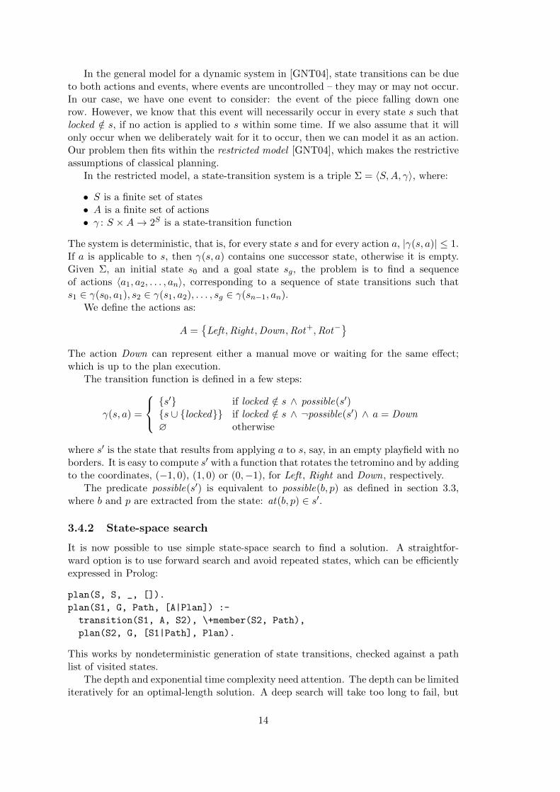
In the general model for a dynamic system in [GNT04], state transitions can be dueto both actions and events, where events are uncontrolled – they may or may not occur.In our case, we have one event to consider: the event of the piece falling down onerow. However, we know that this event will necessarily occur in every state s such thatlocked /∈ s, if no action is applied to s within some time. If we also assume that it willonly occur when we deliberately wait for it to occur, then we can model it as an action.Our problem then fits within the restricted model [GNT04], which makes the restrictiveassumptions of classical planning.

In the restricted model, a state-transition system is a triple Σ = 〈S,A, γ〉, where:

• S is a finite set of states• A is a finite set of actions• γ : S ×A → 2S is a state-transition function

The system is deterministic, that is, for every state s and for every action a, |γ(s, a)| ≤ 1.If a is applicable to s, then γ(s, a) contains one successor state, otherwise it is empty.Given Σ, an initial state s0 and a goal state sg, the problem is to find a sequenceof actions 〈a1, a2, . . . , an〉, corresponding to a sequence of state transitions such thats1 ∈ γ(s0, a1), s2 ∈ γ(s1, a2), . . . , sg ∈ γ(sn−1, an).

We define the actions as:

A ={Left ,Right ,Down,Rot+,Rot−

}The action Down can represent either a manual move or waiting for the same effect;which is up to the plan execution.

The transition function is defined in a few steps:

γ(s, a) =

{s′} if locked /∈ s ∧ possible(s′){s ∪ {locked}} if locked /∈ s ∧ ¬possible(s′) ∧ a = Down∅ otherwise

where s′ is the state that results from applying a to s, say, in an empty playfield with noborders. It is easy to compute s′ with a function that rotates the tetromino and by addingto the coordinates, (−1, 0), (1, 0) or (0,−1), for Left , Right and Down, respectively.

The predicate possible(s′) is equivalent to possible(b, p) as defined in section 3.3,where b and p are extracted from the state: at(b, p) ∈ s′.

3.4.2 State-space search

It is now possible to use simple state-space search to find a solution. A straightfor-ward option is to use forward search and avoid repeated states, which can be efficientlyexpressed in Prolog:

plan(S, S, _, []).

plan(S1, G, Path, [A|Plan]) :-

transition(S1, A, S2), \+member(S2, Path),

plan(S2, G, [S1|Path], Plan).

This works by nondeterministic generation of state transitions, checked against a pathlist of visited states.

The depth and exponential time complexity need attention. The depth can be limitediteratively for an optimal-length solution. A deep search will take too long to fail, but

14

there are many ways to improve on this with plan restrictions that can be used in pruningthe search space. For example, it is extremely unlikely that more than two rotations (ineither direction) are needed.

There is a simple admissible heuristic. Consider moving the piece without obstacles.The optimal solution cost (number of actions) of the relaxed problem is easy to compute:column distance + row distance + number of rotations. Rows below the goal can beexcluded from the search.

A simple technique is to only follow optimal paths as guided by the heuristic. Thisway, the search will be much more predictable, but completeness is sacrificed. This isstill quite acceptable in Tetris, as plans that cannot be found involve unusual goals.Longer paths are also possible to find using subgoals (e.g. near the original goal); seesection 3.7.3 on page 21 for an example.

3.5 Goal generation

The agent needs to have some good knowledge of Tetris in order to find a good goalposition. Then it can reason about candidate goals until it is ready to choose the bestone. If there is not enough time, it should choose a goal in a hurry.

The deadline that we consider here is in terms of external “Tetris time.” A goalmust be chosen before the distance to the blocks below is less than three rows (or someother number) as shown in Figure 3.6.

2 4 6 8 1022

20

18

16

14

12

10

8

6

4

2

L1 at (4, 19)

deadline:

L1 at (4, 6)

· · ··

· · ··

(a)

· · ··

(b)

· · ··

(c)

Figure 3.6: Goal deliberation deadline and goal position examples

We have only built some basic knowledge that allows to generate positions that don’tcreate holes below the piece. A hole is any empty cell that has some block above it inthe same column. For example, placing L1 on a flat surface will give two holes.

Figure 3.6 shows two positions that are generated. The one in (a) should be avoidedfor two reasons: it increases the height; and it creates an empty column deeper thantwo cells, which can only be filled with an I piece. The position in (b) seems to createa hole, but it clears the line above it; (c) shows the result.

15

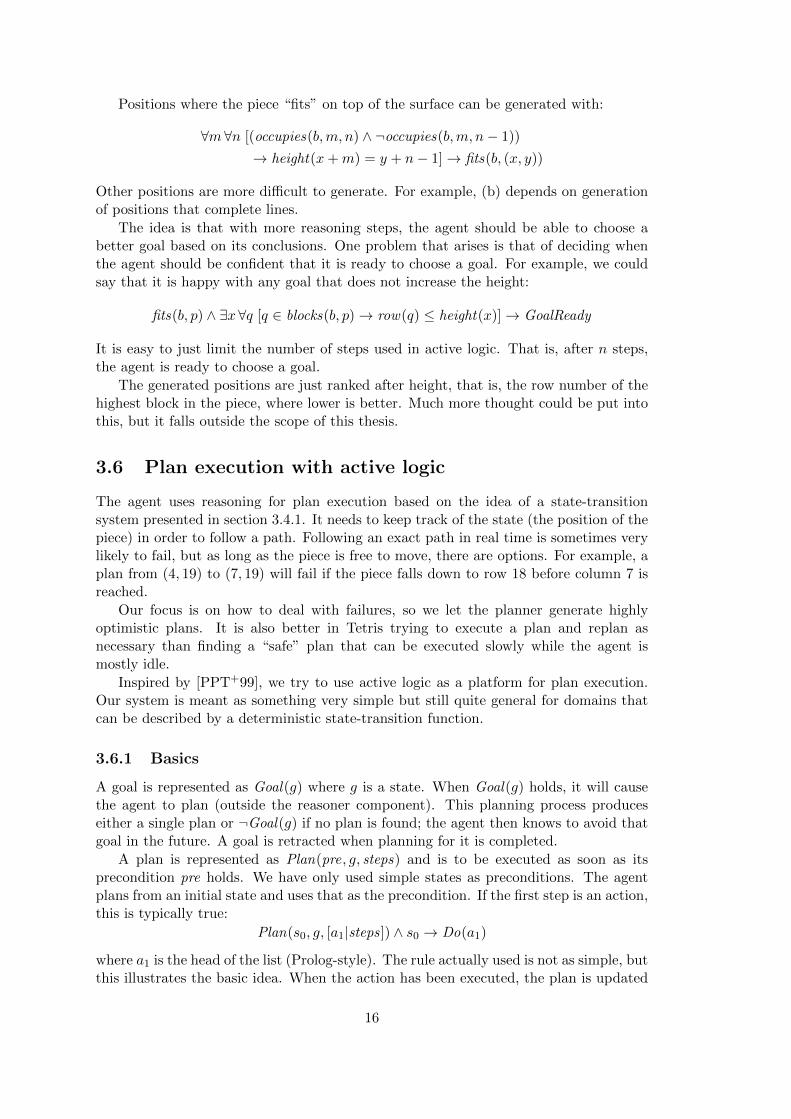
Positions where the piece “fits” on top of the surface can be generated with:

∀m∀n [(occupies(b,m, n) ∧ ¬occupies(b,m, n− 1))

→ height(x+m) = y + n− 1] → fits(b, (x, y))

Other positions are more difficult to generate. For example, (b) depends on generationof positions that complete lines.

The idea is that with more reasoning steps, the agent should be able to choose abetter goal based on its conclusions. One problem that arises is that of deciding whenthe agent should be confident that it is ready to choose a goal. For example, we couldsay that it is happy with any goal that does not increase the height:

fits(b, p) ∧ ∃x∀q [q ∈ blocks(b, p) → row(q) ≤ height(x)] → GoalReady

It is easy to just limit the number of steps used in active logic. That is, after n steps,the agent is ready to choose a goal.

The generated positions are just ranked after height, that is, the row number of thehighest block in the piece, where lower is better. Much more thought could be put intothis, but it falls outside the scope of this thesis.

3.6 Plan execution with active logic

The agent uses reasoning for plan execution based on the idea of a state-transitionsystem presented in section 3.4.1. It needs to keep track of the state (the position of thepiece) in order to follow a path. Following an exact path in real time is sometimes verylikely to fail, but as long as the piece is free to move, there are options. For example, aplan from (4, 19) to (7, 19) will fail if the piece falls down to row 18 before column 7 isreached.

Our focus is on how to deal with failures, so we let the planner generate highlyoptimistic plans. It is also better in Tetris trying to execute a plan and replan asnecessary than finding a “safe” plan that can be executed slowly while the agent ismostly idle.

Inspired by [PPT+99], we try to use active logic as a platform for plan execution.Our system is meant as something very simple but still quite general for domains thatcan be described by a deterministic state-transition function.

3.6.1 Basics

A goal is represented as Goal(g) where g is a state. When Goal(g) holds, it will causethe agent to plan (outside the reasoner component). This planning process produceseither a single plan or ¬Goal(g) if no plan is found; the agent then knows to avoid thatgoal in the future. A goal is retracted when planning for it is completed.

A plan is represented as Plan(pre, g, steps) and is to be executed as soon as itsprecondition pre holds. We have only used simple states as preconditions. The agentplans from an initial state and uses that as the precondition. If the first step is an action,this is typically true:

Plan(s0, g, [a1|steps]) ∧ s0 → Do(a1)

where a1 is the head of the list (Prolog-style). The rule actually used is not as simple, butthis illustrates the basic idea. When the action has been executed, the plan is updated

16

to Plan(s1, g, steps) where s1 is the following state of the corresponding transition andsteps are the remaining steps.

An action here is just a symbol (see section 3.2.2). A step may also be a subgoalof the form Goal(s) which will initiate another plan (if found). When the subgoal hasbeen planned for, the plan progress is updated:

Plan(α, g, [Goal(s)|steps]) ∧ Plan(β, s, γ) → Plan(s, g, steps)

The old plan, whose first step is completed, is retracted.

Rather than waiting for a percept (an observation in active logic), the agent infersthe state from its knowledge of the world:

Do(a) ∧ s1 ∧ transition(s1, a, s2) → s2

This amounts to acting with “closed eyes,” assuming determinism. In addition, theagent does use percepts, that may contradict its conclusions. Neither is really fullyreliable in the architecture due to latency.

3.6.2 Inconsistent beliefs

One aspect of active logic is that it can model a fallible reasoning agent, which is expectedto hold inconsistent beliefs at times. Even when a contradiction is noted and resolved,inconsistent beliefs can make things difficult while they exist. Consider this example,where the first action in the plan is executed:

t : Plan(s0, g, [a1|steps]), s0, transition(s0, a1, s1)...

t+ 2: Plan(s1, g, steps), s1, Plan(s0, g, [a1|steps]), s0, . . .

The action a1 will then get executed again if one is careless.

Unfortunately, there is no obvious way to deal with this kind of problem in activelogic and also keep the rules and axioms as simple as we would like. We can recognisetwo approaches (that may work together):

• Inconsistency is prevented with careful retraction.

• Rules and axioms need to be written carefully so that they don’t conclude anythingharmful from inconsistent beliefs.

The first approach can work by a complicated rule of inheritance. The second approachis more safe, but appears as difficult. We need to take into account that complicatedformulae will not work in our implementation.

It seems natural to view some rules as relevant only in a certain state of consistency.We have come up with a solution that uses a special inference rule to mark a belief setas consistent when there are no contradictory positions in it. This allows us to expressthat a single state holds with:

at(b, p) ∧ Consistent

17

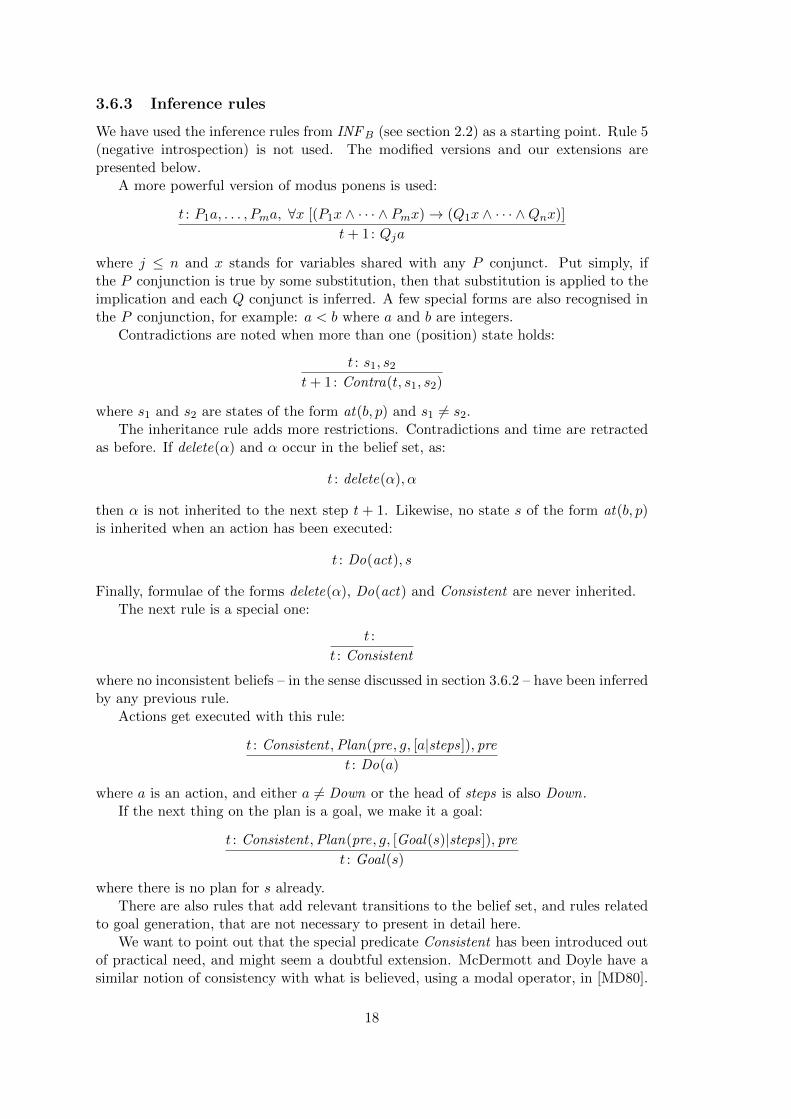
3.6.3 Inference rules

We have used the inference rules from INFB (see section 2.2) as a starting point. Rule 5(negative introspection) is not used. The modified versions and our extensions arepresented below.

A more powerful version of modus ponens is used:

t : P1a, . . . , Pma, ∀x [(P1x ∧ · · · ∧ Pmx) → (Q1x ∧ · · · ∧Qnx)]

t+ 1: Qja

where j ≤ n and x stands for variables shared with any P conjunct. Put simply, ifthe P conjunction is true by some substitution, then that substitution is applied to theimplication and each Q conjunct is inferred. A few special forms are also recognised inthe P conjunction, for example: a < b where a and b are integers.

Contradictions are noted when more than one (position) state holds:

t : s1, s2t+ 1: Contra(t, s1, s2)

where s1 and s2 are states of the form at(b, p) and s1 6= s2.The inheritance rule adds more restrictions. Contradictions and time are retracted

as before. If delete(α) and α occur in the belief set, as:

t : delete(α), α

then α is not inherited to the next step t + 1. Likewise, no state s of the form at(b, p)is inherited when an action has been executed:

t : Do(act), s

Finally, formulae of the forms delete(α), Do(act) and Consistent are never inherited.The next rule is a special one:

t :

t : Consistent

where no inconsistent beliefs – in the sense discussed in section 3.6.2 – have been inferredby any previous rule.

Actions get executed with this rule:

t : Consistent ,Plan(pre, g, [a|steps]), pret : Do(a)

where a is an action, and either a 6= Down or the head of steps is also Down.If the next thing on the plan is a goal, we make it a goal:

t : Consistent ,Plan(pre, g, [Goal(s)|steps]), pret : Goal(s)

where there is no plan for s already.There are also rules that add relevant transitions to the belief set, and rules related

to goal generation, that are not necessary to present in detail here.We want to point out that the special predicate Consistent has been introduced out

of practical need, and might seem a doubtful extension. McDermott and Doyle have asimilar notion of consistency with what is believed, using a modal operator, in [MD80].

18

3.6.4 Axioms

Now we have inference rules that allow us to write robust plan execution axioms quiteeasily. Here follow some examples.

The plan is updated when its first step (an action) is completed:

Plan(s0, g, [a|steps]) ∧ transition(s0, a, s1) ∧DONE

→ Plan(s1, g, steps) ∧ delete(Plan(s0, g, [a|steps]))

where DONE stands for either s0 ∧ Do(a) or s1 ∧ Consistent . That is, two axioms aregenerated. Note that Do(a) implies that the belief set is consistent.

When the goal has been reached, we delete the plan:

Plan(pre, g, steps) ∧ g ∧ Consistent → delete(Plan(pre, g, steps))

State contradictions are resolved with simple axioms. The most trivial one ariseswhen the piece falls down one row:

Now(t) ∧ Contra(t− 1, s1, s2) ∧ transition(s1,Down, s2) → s2

A plan is considered to have failed when its precondition is impossible, which is easyto detect in Tetris:

Plan(at(b, (x, y)), g, steps) ∧ at(b1, (x1, y1)) ∧ Consistent ∧y1 < y → Failed(at(b, (x, y)), g)

Another plan failure is when planning for a subgoal has failed:

Plan(pre, g, [Goal(s)|steps]) ∧ ¬Goal(s) → Failed(pre, g) ∧ ¬Goal(g)

The easiest way to deal with a failed plan is to delete it (and other plans) and replan,possibly for the same goal. It may be better to try and use an existing plan, with littleor no change in the list of steps, from a new initial state.

3.7 Scenarios

Here are three simple Tetris scenarios that show how the agent handles some detailsusing active logic. First are two examples of state contradictions, and then a planinvolving a subgoal is executed.

at(Z1, (5, 19)) s1 at(Z1, (6, 19))s2

at(Z1, (5, 18)) s3 at(Z1, (6, 18))s4

Figure 3.7: The piece falls down while it is moved

19

3.7.1 State contradiction 1

In this setting the piece is about to fall just when an action is executed. There areno obstacles, so the action will succeed in practice. Figure 3.7 shows the states andtransitions involved. The bold arrows indicate the transitions that actually take placein the environment. The most relevant beliefs at each step are shown below:

0: Do(Right), at(Z1, (5, 19)), transition(at(Z1, (5, 19)),Right , at(Z1, (6, 19)))

1 : at(Z1, (6, 19))

2 : at(Z1, (6, 19)), at(Z1, (5, 18))

3 : Contra(2, s2, s3), s2, s3, transition(s1,Right , s2), transition(s1,Down, s3),transition(s3,Right , s4)

4 : s4

The piece falls down one row before Right gets executed in the game, which normallymeans that the action takes place in the observed state s3 ∈ OBS (2). The contradictionis resolved with this axiom:

Now(t) ∧ Contra(t− 1, s2, s3) ∧ transition(s1, a, s2) ∧transition(s1,Down, s3) ∧ transition(s3, a, s4) → s4

Note that s2 and s3 are not inherited from step 3 as they have been noted in a con-tradiction. Modus ponens concludes s4 from Now(3), the contradiction and transitionsshown at step 3 and the axiom above.

3.7.2 State contradiction 2

The agent tries to rotate clockwise, from T1 to T2, but the game rotates the piece in theopposite direction (see Figure 3.8). The reason might be that the game is stochastic, orthat it only rotates in one direction. A contradiction is noted between at(T2, (4, 9)) andat(T4, (4, 8)) a few steps later, when the correct state has been observed. This kind ofcontradiction can be resolved with:

Now(t) ∧ Contra(t− 1, at(b1, (x, y)), at(b2, (x, y − 1))) → at(b2, (x, y − 1))

The real problem is then to replan without repeating the same mistake, which be-comes even more difficult if we consider that the piece could have been rotated morethan once before any observation is received. A basic idea is to do rotate repeatedly,until the right orientation is observed; however, we will not attempt to go further andtackle any technical issues.

at(T4, (4, 9)) s3 s1

at(T1, (4, 9))

at(T2, (4, 9))s2

at(T4, (4, 8)) s4

Figure 3.8: Rotation in wrong direction

20

2 4 6 8 10

8

6

4

2

· ·· ·

· ·· ·

2 4 6 8 10

8

6

4

2· ·· ·

2 4 6 8 10

8

6

4

2

Figure 3.9: Planning using a subgoal

3.7.3 Plan with a subgoal

Figure 3.9 shows a goal which the planner cannot find directly. It falls back on backwardsearch to a subgoal – a positon where the piece is above the surface (the height of eachcolumn) – and a plan of the following list of steps is generated:

[Right ,Goal(at(Z1, (8, 2))),Down,Left ,Left ]

Another plan to reach the subgoal is then needed, as soon as the first action has beenexecuted. Here is a selection of beliefs that we expect:

0 : at(Z1, (4, 7)), Goal(g)

1 : Do(Right)

2 : Goal(at(Z1, (8, 2)))

3 : Plan(at(Z1, (5, 7)), at(Z1, (8, 2)), [Right , . . . ,Down]),Plan(at(Z1, (8, 2)), g, [Down,Left ,Left ])

21

Chapter 4

The theorem prover

4.1 Background

Julien Delnaye implemented a theorem prover in Prolog [Del08], which, in particular, wasmeant to be used with active logic as formalised in [Ask03]. It also allowed customisationfor other logical systems based on LDS (see section 2.3). Our work has aimed at a moreefficient prover with basically the same functionality.1

First, we looked for sources of inefficiency. The program operates repeatedly on inputin the form of lists of beliefs, observations and inference rules, producing as output anew list of beliefs, which is then used as input in the next iteration. The most apparentproblem in the case of the robot-day scenario is that the same list of observations (morethan a thousand items) is processed in every iteration. It is obvious that an observationonly needs to be looked at once, at the time it is new (and not before it has been made).This could be solved without much effort though, at the same time allowing input ofobservations in-between the reasoning steps.

Actually, we never got any deeper into the code, which was very hard to understand.However, the heavy use of recursion on lists is suspected. In many places intermediatelists are created and concatenated in an inefficient way. Just fixing these would furtherobfuscate the code.

Instead, the program was entirely rewritten, after it was realised that most of thetheorem proving could be done by Prolog. Our approach is actually quite similar toElgot-Drapkin’s in the Prolog code to solve (for example) the Brother problem [ED88],which we did not look at initially.

4.2 Overview

Here we describe how the new prover is used and the basics of how it works. Someacquaintance with Prolog is recommended. Predicates are referred to as name/n, wheren is the arity (number of arguments).

The prover is typically loaded inside another Prolog program, which defines a numberof facts that provide the specification to the prover. It basically needs to know threethings: the structure used to hold a belief, the inference rules, and, at each time step,the new observations.

1LDS support is less general in that labels are required to hold a time point which is used as in activelogic.

22

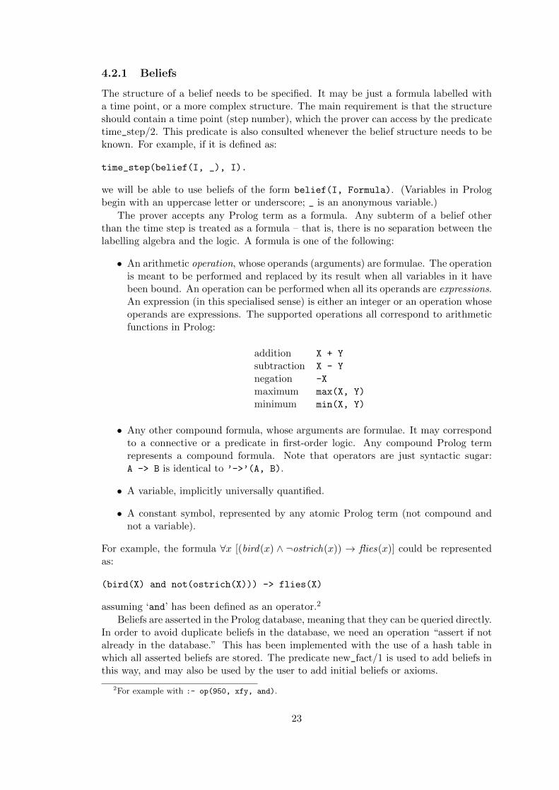
4.2.1 Beliefs

The structure of a belief needs to be specified. It may be just a formula labelled witha time point, or a more complex structure. The main requirement is that the structureshould contain a time point (step number), which the prover can access by the predicatetime_step/2. This predicate is also consulted whenever the belief structure needs to beknown. For example, if it is defined as:

time_step(belief(I, _), I).

we will be able to use beliefs of the form belief(I, Formula). (Variables in Prologbegin with an uppercase letter or underscore; _ is an anonymous variable.)

The prover accepts any Prolog term as a formula. Any subterm of a belief otherthan the time step is treated as a formula – that is, there is no separation between thelabelling algebra and the logic. A formula is one of the following:

• An arithmetic operation, whose operands (arguments) are formulae. The operationis meant to be performed and replaced by its result when all variables in it havebeen bound. An operation can be performed when all its operands are expressions.An expression (in this specialised sense) is either an integer or an operation whoseoperands are expressions. The supported operations all correspond to arithmeticfunctions in Prolog:

addition X + Y

subtraction X - Y

negation -X

maximum max(X, Y)

minimum min(X, Y)

• Any other compound formula, whose arguments are formulae. It may correspondto a connective or a predicate in first-order logic. Any compound Prolog termrepresents a compound formula. Note that operators are just syntactic sugar:A -> B is identical to ’->’(A, B).

• A variable, implicitly universally quantified.

• A constant symbol, represented by any atomic Prolog term (not compound andnot a variable).

For example, the formula ∀x [(bird(x) ∧ ¬ostrich(x)) → flies(x)] could be representedas:

(bird(X) and not(ostrich(X))) -> flies(X)

assuming ‘and’ has been defined as an operator.2

Beliefs are asserted in the Prolog database, meaning that they can be queried directly.In order to avoid duplicate beliefs in the database, we need an operation “assert if notalready in the database.” This has been implemented with the use of a hash table inwhich all asserted beliefs are stored. The predicate new_fact/1 is used to add beliefs inthis way, and may also be used by the user to add initial beliefs or axioms.

2For example with :- op(950, xfy, and).

23

4.2.2 Inference rules

An inference rule has the form rule(Premises, Conclusion) where Premises is a listof premises. Conclusion has the structure of a belief. For example, modus ponens inactive logic can be defined as:

rule([belief(I, A), belief(I, A->B)], belief(I+1, B)).

A premise is almost the same as a Prolog goal but may contain arithmetic operationsjust like formulae in beliefs. There are also two premise goals that are given specialstatus:

• a belief goal that has the structure of a belief;• an observation goal of the form obs(I, Formula), analogous to α ∈ OBS (i).

They are recognised inside negation (as failure) as well, either with:

\+ Goal or not(Goal).

Variables in goals should generally be understood as implicitly existentially quanti-fied over the body they appear in – we may say over the rule here. A solution is the sameas a binding of the variables in a goal. One thing to keep in mind is that all solutionsin premise goals will be generated, so code that leaves a lot of choice points around willmake the rule inefficient.

The inference rules are applied to the history to bring conclusions at a given timestep. They may start from any belief or observation in the history. For example, ifapply_rule/2 is called as apply_rule(5, _), it will pick a rule and make the time stepin the conclusion equal to 5, as in this query:

?- rule(Prems,Concl), time_step(Concl,I), eq(5,I).

It may be necessary to solve a trivial equation like 5 = x + 1, which is done by eq/2.Then the premises are ready to be proven.

The old prover works the other way around, binding the time variable only byprocessing the premises. This is not only less flexible, but requires rules to be writtenin an inefficient way (both in terms of performance and typing). In contrast, no premisethat binds the time variable is needed here. For example, the “clock axiom” may bedefined simply as:

rule([], belief(I, now(I))).

Also, these two rules are equivalent:

rule([belief(I, A)], belief(I+1, A)).

rule([belief(I-1, A)], belief(I, A)).

The order in which the rules are applied has significance if any rule uses premises ofthe same time step as its conclusion. All the conclusions of one rule are produced beforeany following rule is applied, as expected. The conclusions of one rule are visible in thehistory – that is, premises can use them – when the following rules are applied, but thesame rule cannot see its own conclusions until one step later.3

3This behaviour is due to the logical update view in Prolog; when backtracking over the beliefs in thedatabase, changes to the belief predicate are not seen.

24

We can see that this is a sort of incomplete reasoning that may not be desired. Theapplication of the rules could be repeated until no new beliefs are produced; however,we prefer to keep the prover simple and efficient for step-wise reasoning.

This is also a point where the old prover is quite different. Rules that don’t incrementthe time are only applied to the same immutable list of beliefs, “the intermediate beliefset,” producing a second list of beliefs. The two lists are then concatenated to formthe belief set of the completed step. In comparison, our prover can be said to update adynamic intermediate belief set every time it advances to the next rule.

4.2.3 History

Active logic defines a history as a sequence with all the belief sets and observation setsup to a certain time point. We give the concept of history a specific meaning in theimplementation: “the history” refers to the beliefs and observations in the databasesof the prover (the Prolog databases and the hash table). The idea is that only (andall) those previous steps that are actually used to produce the next belief set shouldbe kept in memory. That is, the output should be same as if the prover used a historycontaining all the previous steps.

The history size is the number of (consecutive) steps to remember after all inferencerules have been applied. When the history grows beyond this size, the oldest step isfreed. For the inference function INFB described in section 2.2, a history size 1 issufficient, which is defined as:

history_size(1).

A larger size is needed if any rule looks beyond the previous step.

4.2.4 Observations

The easiest way to provide observations in a static way is to define the predicate obs/2directly. For example:

obs(0, bird(tweety)).

obs(4, ostrich(tweety)).

If obs/2 is undefined, observations are looked for in the recorded database, usingthe time step as key. These observations are also removed when they fall outside the(limited) history. Observations can be added directly, as in:

:- recordz(0, bird(tweety)).

But the intended usage is to define a special predicate, observations/2, that behaves ac-cording to its description in section 4.3.2. At the beginning of each step, observations/2is called once. The returned list of observations is expected to contain all observationsthat have been made since the last call. Each belief is recorded under the current timestep.

4.3 Predicate descriptions

Here the most important predicates for the user are described. Arguments are sometimespreceded by a mode indicator: (+) means that the argument is used as input (it mustbe instantiated) and (-) that it is used as output.

25

4.3.1 Basic predicates

step(I ) runs the next reasoning step, producing beliefs at time I by backtracking overapply_rule/2. If instantiated, I should be a natural number equal to the previousstep plus one, or, if this is the first step, either 0 or 1. The new belief set is printedto the current output stream.

Here is an example that will run until step 5 is completed:

?- repeat, step(I), I=5.

reset frees all the history and goes back to step 0.

apply_rule(+I, -Belief ) infers one new belief at time step I and returns it in Belief.It picks a rule with rule/2 and proves its premises, nondeterministically. Then itasserts the conclusion with new_fact/1.

query(+Goal) proves Goal, with special handling of beliefs and observations. It is usedin proving premises, and is an appropriate place to add more functionality.

Proving a belief goal may involve arithmetic evaluation and inverse operations.For example:

?- query(belief(0, plus(1,X,3))), belief(0, plus(Y,Z,Y+Z)).

X = 2.

all(+Cond, +Prem) generates a list of premises and proves them in the same way asapply_rule/2. For each solution of Cond, a copy of Prem is added with the bindingsfrom the solution.

This predicate is specifically used in the extended modus ponens rule and is alsogenerally useful. Let us take the example of proving a conjunction:

Ps = bird(X) and not(ostrich(X)),

all(conjunct(P,Ps), P).

The generated list of premises is then:

[bird(X), not(ostrich(X))]

conjunct(P, Ps) is true if P is a conjunct in Ps. It can choose an element nondetermin-istically from a conjunction built with and/2 lists. If Ps cannot be unified withand(_,_) then it is considered to be a conjunction with a single conjunct.

?- conjunct(p, p).

true.

?- conjunct(X, and(p, and(q, r))).

X = p ;

X = q ;

X = r ;

false.

26

csf(A, +B) generates closed subformulae: A is a closed subformula of B. Any subterm(including B) that is not one of the following is considered a closed subformula:

• a variable;• a number;• a term that shares variables with other subterms of B (that are not subterms

of itself).

4.3.2 User-defined predicates

These predicates need to be written by the user and should be in accordance with theirdescriptions.

time_step(Belief, I ) is true if Belief has the structure of a belief or is an unboundvariable, and I can be unified with the subterm that holds the time step. Beliefshould be unified with a term that has the structure of a belief (a skeleton).

It must be possible to assert a belief dynamically (with assertz/1). It is recom-mended that the user declares the belief predicate as dynamic, for example, withthis line:

:- dynamic belief/2.

rule(-Prems, -Concl) returns an inference rule: a list of premise goals in Prems andthe conclusion (a belief structure) in Concl.

obs(+I, -Formula) returns an observation at time I in Formula.

If observations are static, it is easy to define this predicate with a set of facts.Define either obs/2 or observations/2, not both.

observations(+I, -Obs) returns a list of new observations (formulae) in Obs. If thereare no new observations, Obs=[].

observations/2 should be seen as a procedure that reads observations from theoutside world everytime it is called. The observations are considered to have beenmade at time I, but this argument may be ignored.

4.3.3 Database

These predicates use the clause database as a set without duplicate facts (clauses willalso work). Terms are hashed with term_hash/2 and stored in a “bucket array” that iswritten in C and uses SWI-Prolog’s foreign language interface.

new_fact(+Fact) asserts Fact in the database (with assertz/1) and adds it to the hashtable. True if Fact is new and fails if it’s already in the hash table.

element(+Fact) is true if Fact is an element of the database set, that is, identical to aterm in the hash table (except for renaming of variables).

delete_facts(+Fact) deletes all facts that unifies with Fact.

27

Chapter 5

Results

5.1 Theorem prover examples

Julien Delnaye demonstrated his program on three simple problems, the wise men prob-lems from [ED88] and the Tweety problem from [Ask03]. We have verified that the newtheorem prover is able to take the same problems, specified much the same way, andsolve them correctly.

5.1.1 Implementation

The Two-wise-men problem (2WM) was straightforward to translate and check againstthe original definition after we had implemented an extended modus ponens rule (seeAppendix A and the descriptions of all/2 and conjunct/2 in section 4.3.1).

The Three-wise-men problem (3WM) did not require any further extensions; how-ever, there was some confusion from a couple of rules that were left out – apparently,this just leads to a slightly different solution. No significant differences between theimplementations could be seen in the output, with respect to how rules behaved.1

The Tweety problem uses some complicated rules that were implemented using aux-iliary Prolog code. The output is now quite identical to Asker’s proof, whereas a fewissues were discovered in Delnaye’s implementation. In particular, some forumulae arenot properly instantiated. For example, at step 2, where ¬K(2,¬flies(Tweety)) is expec-ted (the agent does not know that Tweety cannot fly), ∀x ¬K(2,¬flies(x)) is producedinstead (the agent does not know that any object cannot fly), which is not the samething, although it will do no harm here.

5.1.2 Performance

Table 5.1 shows system statistics as reported by Prolog immediately after the last stephas finished. This simple method is sufficient to show a clear difference in performance,even if the various memory areas are unfamiliar, since the crude measures differ so much.The tests were run using the 32-bit version of SWI-Prolog in Linux.

Next is a description of the columns, followed by some remarks and additional in-formation.

The number of steps shown is the number of belief sets produced. Speed is indicatedby CPU time in seconds and the number of inferences in thousands. Memory require-

1There were, however, a few mistyped axioms in Delnaye’s code.

28

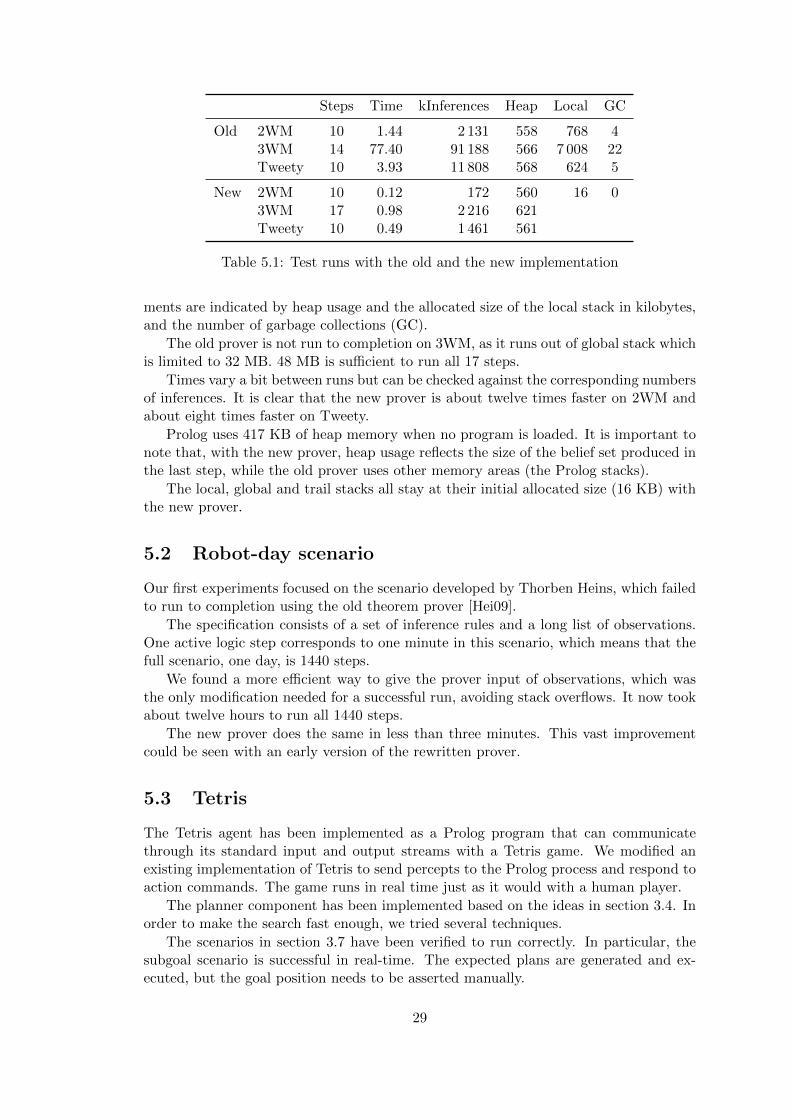
Steps Time kInferences Heap Local GC

Old 2WM 10 1.44 2 131 558 768 43WM 14 77.40 91 188 566 7 008 22Tweety 10 3.93 11 808 568 624 5

New 2WM 10 0.12 172 560 16 03WM 17 0.98 2 216 621Tweety 10 0.49 1 461 561

Table 5.1: Test runs with the old and the new implementation

ments are indicated by heap usage and the allocated size of the local stack in kilobytes,and the number of garbage collections (GC).

The old prover is not run to completion on 3WM, as it runs out of global stack whichis limited to 32 MB. 48 MB is sufficient to run all 17 steps.

Times vary a bit between runs but can be checked against the corresponding numbersof inferences. It is clear that the new prover is about twelve times faster on 2WM andabout eight times faster on Tweety.

Prolog uses 417 KB of heap memory when no program is loaded. It is important tonote that, with the new prover, heap usage reflects the size of the belief set produced inthe last step, while the old prover uses other memory areas (the Prolog stacks).

The local, global and trail stacks all stay at their initial allocated size (16 KB) withthe new prover.

5.2 Robot-day scenario

Our first experiments focused on the scenario developed by Thorben Heins, which failedto run to completion using the old theorem prover [Hei09].

The specification consists of a set of inference rules and a long list of observations.One active logic step corresponds to one minute in this scenario, which means that thefull scenario, one day, is 1440 steps.

We found a more efficient way to give the prover input of observations, which wasthe only modification needed for a successful run, avoiding stack overflows. It now tookabout twelve hours to run all 1440 steps.

The new prover does the same in less than three minutes. This vast improvementcould be seen with an early version of the rewritten prover.

5.3 Tetris

The Tetris agent has been implemented as a Prolog program that can communicatethrough its standard input and output streams with a Tetris game. We modified anexisting implementation of Tetris to send percepts to the Prolog process and respond toaction commands. The game runs in real time just as it would with a human player.

The planner component has been implemented based on the ideas in section 3.4. Inorder to make the search fast enough, we tried several techniques.

The scenarios in section 3.7 have been verified to run correctly. In particular, thesubgoal scenario is successful in real-time. The expected plans are generated and ex-ecuted, but the goal position needs to be asserted manually.

29

There is nothing very impressive about the Tetris-playing abilities of our system,and we have not much discussed methods to measure its success. That is also not thepoint of this thesis. The Tetris AI is incomplete in many ways.

Reliable real-time plan execution using active logic was hard to achieve with ourapproach. At higher speeds the agent is unable to determine the position of the piece andwill not act at all. This is because it receives contradictory observations too frequently– some number of active logic steps is needed to handle each such event.

The planner is called between execution of active logic steps, in the same thread,usually several times before the goal position is reached. Plan generation is actuallyquite fast, but too much replanning (every time the piece falls down one row), whichalso involves reasoning, is a trouble that may slow down plan execution awkwardly. Toaccommodate this, we generate one plan in advance, from the position one row below,which gives a significant improvement.

Another issue is that reasoning gets slower as the belief set grows in each step.Our workaround is to reset the theorem prover every time a new piece is played, butsometimes the agent will still get very slow.

30

Chapter 6

Conclusions

We have shown that the theorem prover could be made much more efficient, in terms ofspeed and memory usage, while keeping its flexibility, which was questioned in [Del08].Also, although it was rewritten from scratch, this did not require as much work as wefirst thought. We found that much of the functionality that [Del08] implemented wasalready in Prolog and could be used for better performance.

The Tetris agent uses active logic at a low level (e.g. for keeping track of the positionof the piece) which might not be its best use. It has been troublesome to develop asystem that wouldn’t be too disappointing from a Tetris point of view, and also woulduse active logic in a clear way.

Reasoning with an approaching deadline (see section 3.5) has been implemented butnot clearly demonstrated in this report. Simple scenarios that involve contradictionhandling have been presented, but they are not very good examples of its usefulness.

The speed of our new active logic implementations is quite promising; however, theproblem that the set of beliefs can grow very large is still apparent in the robot-dayscenario and sometimes in our Tetris agent (despite some efforts to retract unneededformulae). A short-term memory of limited size, as in the LDS-based formalisation in[Ask03], can still be very useful.

Here are the immediate improvements we envision:

• The theorem prover could be modified to more generally support LDS-like systems.This might only require changes that avoid the special treatment of time points.

• The prover needs additions that involve new syntax for some logical symbols, forexample, in order to support quantified subformulae.

• The Tetris agent’s reasoning about goal positions is very basic. It would be inter-esting to see something that clearly leads to better decisions as more time is spenton reasoning.

Prolog programs and other code is available at:http://fileadmin.cs.lth.se/ai/xj/VictorNilsson/alcode.tar.gz

31

Bibliography

[Ask03] M. Asker. Logical Reasoning with Temporal Constraints. Master’s Thesis,Department of Computer Science, Lund University, 2003.

[Del08] J. Delnaye. Automatic Theorem Proving in Active Logics. Master’s thesis,Department of Computer Science, Faculty of Engineering, Lund University,2008.

[ED88] J. Elgot-Drapkin. Step-logic: Reasoning Situated in Time. PhD thesis, De-partment of Computer Science, University of Maryland, 1988.

[EDP90] J. Elgot-Drapkin, D. Perlis. Reasoning Situated in Time I: Basic Con-cepts. Journal of Experimental and Theoretical Artificial Intelligence, 2:75–98, 1990.

[FH88] R. Fagin and J.Y. Halpern. Belief, Awareness, and Limited Reasoning. Ar-tificial Intelligence, 34:39–76, 1988.

[GNT04] M. Ghalab, D. Nau, and P. Traverso. Automated Planning: Theory andPractice. Morgan Kaufmann, 2004.

[Hei09] T.O. Heins. A Case-Study of Active Logic. Master’s thesis, Department ofComputer Science, Lund University, 2009.

[Mal09] J. Malec. Active logic and practice. In proceedings of SAIS 2009, The SwedishAI Society Workshop, pages 49–53. Linkoping University Electronic Press,2009.

[MD80] D. McDermott and J. Doyle. Non-Monotonic Logic I. Artificial Intelligence,13:41–72, 1980.

[Nil91] N.J. Nilsson. Logic and artificial intelligence. Artificial Intelligence, 47:31–56, 1991.

[PPT+99] K. Purang, D. Purushothaman, D. Traum, C. Andersen, and D. Perlis. Prac-tical Reasoning and Plan Execution with Active Logic. In Proceedings of theIJCAI’99 Workshop on Practical Reasoning and Rationality, 1999.

32

Appendix A

Example specification: The Brother problem

Here is a complete Prolog program using our “active logic theorem prover.” It imple-ments all the inference rules of INFB (see section 2.2). Our extended modus ponensrule is more powerful than the original definition and makes Rule 3 unnecessary.

The three scenarios of the Brother problem are presented in [EDP90]. This code willproduce the first scenario – uncomment either of the last lines for the other scenarios.

:- load_files(altp).

:- dynamic belief/2.

:- op(950, xfy, and).

time_step(belief(I,_), I).

rule([], belief(I, now(I))).

rule([obs(I,A)], belief(I, A)).

rule([belief(I, Ps->Q), all(conjunct(P,Ps), belief(I,P))],

belief(I+1, Q)).

rule([belief(I, A), csf(B,A), B \= k(_,_), \+element(belief(I,B))],

belief(I+1, not(k(I, B)))).

rule([belief(I, not(A)), belief(I, A)],

belief(I+1, contra(I, A, not(A)))).

rule([belief(I, A), A \= now(_), \+belief(I, contra(I-1, A, _)),

\+belief(I, contra(I-1, _, A))],

belief(I+1, A)).

obs(0, p -> b).

obs(0, now(X) and not(k(X-1, b)) -> not(b)).

%obs(0, b).

%obs(0, p).

33