ACCURACY STUDY OF FINITE DIFFERENCE METHODS

. a

'1- \

2

)7 p*ibv Nuncv Tune Cvrzcs und Robert E. FzcZton l*s,-k3J J d J ...i - c.-,&

' .-'Tr &._-,

LungZey Reseurch Center :,;?-&.y L . .

,

.

, I,

. . . .\ ILungley Stution, Humptonj vu. - 2

NATIONAL AERONAUTICS A N D SPACE I A D M I N I S T R A T I O N WASHINGTON, D. C. JANUARY 1968

https://ntrs.nasa.gov/search.jsp?R=19680007599 2019-04-10T02:31:23+00:00Z

TECH LIBRARY KAFB. NM

0333477 N A S A 'I" lJ-43'lZ

ACCURACY STUDY O F FINITE DIFFERENCE METHODS

By Nancy J a n e Cyrus and Robert E. Fulton

Langley Resea rch Center Langley Station, Hampton, Va.

NATIONAL AERONAUTICS AND SPACE ADMINISTRATION

For sale by the Clearinghouse far Federal Scientific and Technical Information Springfield, Virginia 22151 - CFSTI price $3.00

ACCURACY STUDY O F FINITE DIFFERENCE METHODS

By Nancy Jane Cyrus and Robert E. Fulton Langley Research Center

SUMMARY

A method for studying the accuracy of finite difference approximations for linear differential equations is presented and utilized. Definitive expressions for the e r r o r in each approximation are obtained by using Taylor se r ies to derive the differential equa­tions which exactly represent the finite difference approximations. The resulting differ­ential equations are accurately solved by a perturbation technique which yields the e r ro r directly.

This method is used t o assess the accuracy of two alternate forms of central finite difference approximations for solving boundary value problems in structural analysis which a r e governed by certain equations containing variable coefficients. A "half station approximation'' in which finite difference approximations a r e made before expanding derivatives of function products is compared with a "whole station approxim@i&' in which derivatives of function products are expanded first for string, beam, and axisymmetric circular plate problems. An example of a square membrane is given as an application of the method to partial differential equations.

INTRODUCTION

The differential equations governing the behavior of structural boundary value prob­lems a r e often solved by approximating the derivatives by finite differences and solving the resulting algebraic equations on a digital computer. For complicated structures the number of simultaneous equations resulting from finite difference approximations can be sufficiently large to exceed the capacity of the computer or introduce round-off e r ror . For such problems, the accuracy of the difference procedure can be a critical item in obtaining meaningful design results. In reference 1, for example, it was found that accu­rate answers for the s t r e s s in a shell could not be obtained by using certain finite differ­ence approximations unless the mesh spacing was smaller than machine capacity permitted.

The most popular difference approximations a r e the so-called central differences which a r e given in textbooks on numerical methods. There are alternate formulations of central differences which can be used when odd order derivatives occur in the differential

equations. Such a situation exists in structural problems, for example, where inplane loads are not uniform (a column loaded by its own weight or a shell of revolution sub­jected to arbitrary loads) or where the stiffness of the structure is nonuniform (a tapered beam or a variable thickness shell).

In this paper a method for studying the accuracy of finite difference approximations is presented and utilized. As illustrative examples, the method is used to assess the accuracy of two alternate forms of central finite difference approximations used in struc­tural problems through application to string, beam, axisymmetric circular plate, and square membrane problems. The same approach can be used t o evaluate the accuracy of finite element methods.

SYMBOLS

linear differential operators

linear difference operators

nondimensional tension in a beam o r string

nondimensional stiffness of beam

finite difference spacing

any integer

superscript describing set of boundary conditions

Fourier wave numbers

nondimensional lateral load

boundary condition

descriptive coordinates of beam, string, plate, or membrane

deflection of beam, string, plate, or membrane

deflection function in perturbation ser ies

slope of plate

boundary curve

Prime or Roman numeral with a symbol denotes differentiation with respect to x.

METHODOFAPPROACH

The usual approach in a finite difference accuracy study is to car ry out the numeri­cal solution to a number of problems for which exact solutions can be obtained and to com­pare the resulting numerical answers at each station with the exact answers. Such a procedure has the liability that comparisons can only be made for each problem at spe­cific stations and the calculations must be redone each time the mesh s ize changes.

The approach used in this paper is to isolate the principal finite difference e r r o r so that its magnitude and character can be evaluated. The finite difference approximations a r e expanded in Taylor ser ies to give differential equations which a r e exactly equivalent to the finite difference approximations. Solving the resulting differential equations by a perturbation technique yields analytical expressions for the principal e r r o r term. These expressions a r e independent of mesh spacing and give a clear indication of the accuracy of the difference approximations not just at discrete points but over the whole domain of interest.

Consider the differential equation

with a necessary and sufficient set of k boundary conditions, each of the form

Equation (1)may represent either an ordinary o r partial differential equation. For example, equation (1) takes the form for a string of

and for a membrane of

3

where V2 is the Laplacian operator

The differential equation (1) is approximated by finite differences and is replaced by a finite difference recursion formula at the ith station of the form

where D(yi) is the equivalent finite difference operator for L(y) and is expressed in te rms of y evaluated at the appropriate finite difference stations.

A similar treatment for each of the k boundary conditions leads to replacing equation (2) by

where Ek is the finite difference operator for Bk. Note that operators of the form of equations (3) and (4) also result for finite element problems if a continuum is approxi­mated by finite elements and the approximate equilibrium equations and boundary condi­tions a re obtained.

The finite difference recursion equations (3) and (4) may be expanded about the ith point by using the appropriate Taylor se r ies expansion, such as the one-dimensional expansion

For any central finite difference method, the order of e r r o r of the approximation is proportional to h2 and the finite difference recursion formula takes the form

where Lo, Ll , and La a r e differential operators which depend on the approximation method used. A similar treatment for Ek leads to

2 k 4 kEk(Yi) = BOk(Yi) + h B1 (Yi) + h B2 (yi) + . . .

For other difference approximations all powers of h may occur.

4

By use of equations (5a) and (5b), the finite difference equations (3) and (4) now take the form

Lo(yi) - pi + h2L1(yi) + h4L2(yi) + . . . = 0 (6)

2 k 4 kBOk(yi) - qik + h B1 (yi) + h B2 (yi) + . . . = 0 (on r) (7)

Equation (6) and its k boundary condition equation (7)are the differential equations which represent the finite difference recursion equations (3) and (4). As the increment h goes to zero, equation (6) and equation (7)should approach equation (1) and equa­tion (2), respectively. In fact, if the finite difference approximations used a r e a con­vergent set, then

Lo = L and

Bo = B

The solution to equations (6) and (7) gives an analytical representation of the numer­ical finite difference answers. Unfortunately, because of the infinite number of te rms in equation (6) a closed form solution does not appear feasible. However, in a practical problem where the size of the region is scaled to be of the order one, h is perhaps 0.1 or 0.01 or even smaller. This small value of h suggests that equation (6) may be solved by a perturbation technique with the perturbation parameter taken to be h2.

Let the solution to equations (6) and (7) be taken in the form

y i = Y o + h2Y l + h4Y 2 + . . . Substituting equation (8) into equation (6) leads to

subject to k boundary conditions of the form

Bok(Yo) - q: + h2[Bgk(Y1) + Blk(Yoj + h4[BOk(Y2)+ Blk(Y1) + B:(Yo)l + . . . = 0

(10) If each order of e r r o r term is solved in sequence, the following ser ies of problems

result:

5

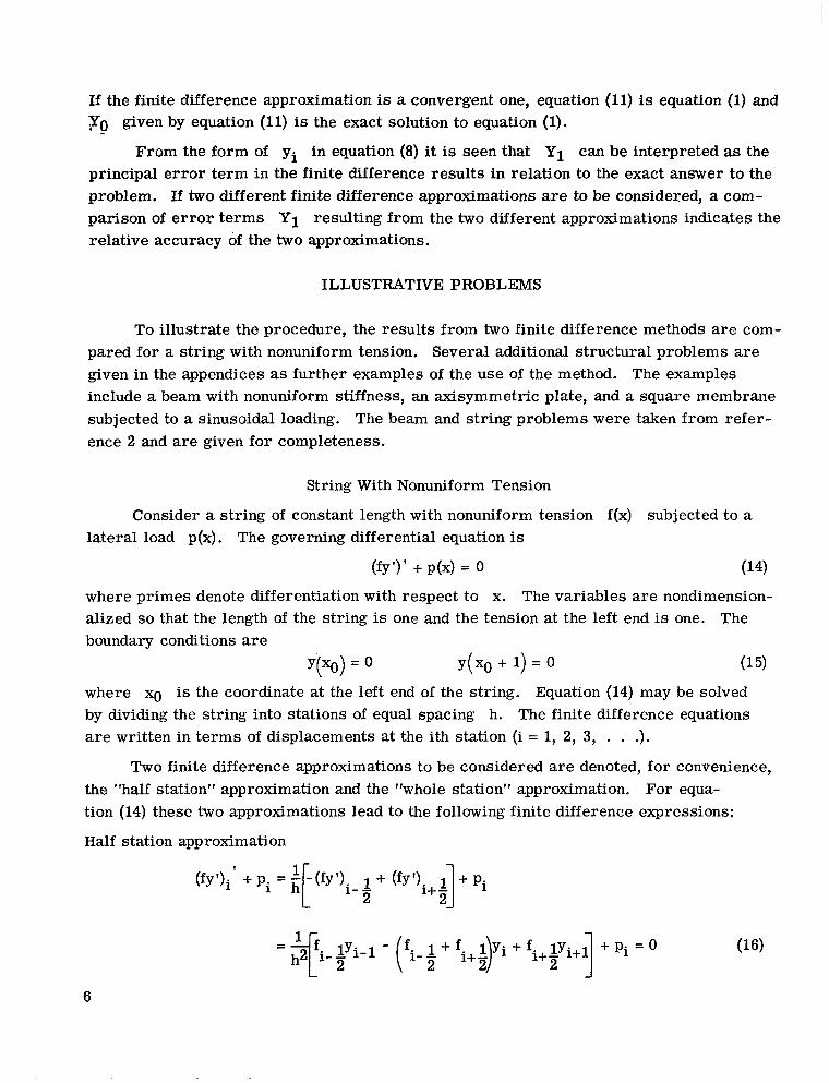
If the finite difference approximation is a convergent one, equation (11) is equation (1) and

;Yo given by equation (11) is the exact solution to equation (1).

From the form of yi in equation (8) it is seen that Y1 can be interpreted as the principal e r r o r te rm in the finite difference results in relation to the exact answer to the problem. If two different finite difference approximations are to be considered, a com­parison of e r r o r te rms Y1 resulting from the two different approximations indicates the relative accuracy of the two approximations.

ILLUSTRATIVE PROBLEMS

To illustrate the procedure, the results from two finite difference methods are com­pared for a string with nonuniform tension. Several additional structural problems are given in the appendices as further examples of the use of the method. The examples include a beam with nonuniform stiffness, an axisymmetric plate, and a square membrane subjected to a sinusoidal loading. The beam and string problems were taken from refer­ence 2 and are given for completeness.

String With Nonuniform Tension

Consider a string of constant length with nonuniform tension f(x) subjected to a lateral load p(x). The governing differential equation is

(fy')' + p(x) = 0 (14)

where primes denote differentiation with respect to x. The variables a r e nondimension­alized so that the length of the string is one and the tension at the left end is one. The boundary conditions are

Y(X0) = 0 y(x0 + 1) = 0 (15)

where xo is the coordinate at the left end of the string. Equation (14) may be solved by dividing the string into stations of equal spacing h. The finite difference equations are written in te rms of displacements at the ith station (i = 1, 2, 3, . . .).

Two finite difference approximations to be considered are denoted, for convenience, the "half station" approximation and the "whole station" approximation. For equa­tion (14) these two approximations lead to the following finite difference expressions:

Half station approximation

6

or whole station approximation

= $[(ti - %)yi-l - 2fiYi + f i + 2yi+l + pi = 0 (17)( "9 ] Note that the half station approximation is the natural result of making the finite differ­ence approximation before expanding the derivatives, whereas the whole station approxi­mation results from making the approximation after the expansion. The latter type of approximation is widely used. (See, for example, refs. 3 and 4.) Both of the preceding se t s of finite difference approximations can be shown to be of order h2 and yet they clearly lead to different coefficients for the simultaneous equations in t e rms of the dis­placements at the ith station. Of concern here a r e the relative magnitudes of the e r r o r s in these two different approximations.

Expand the finite difference recursion equations (16) and (17) about the ith point by using such Taylor se r ies expansions as

n

For both the half station and whole station approximations, this procedure leads to a dif­ferential equation of the form given by equation (6) where

LOtYi) = ( f i Y i I )

Bo(Yi) = Y i

and for the half station approximation

fiYiVI fiIYiV fi"Y;V f i y i l l l fiIVyi" fiVyi'

L2(yi) = xz-+-120

+-96

+ 144 384 1920

J . . .

and for the whole station approximation \

J . . .

Equations (6) and (7) with equations (18) and either equations (19), (20), . . ., or equations (21), (22), . . ., are clearly differential equations and associated boundary con­ditions which represent exactly the two finite difference recursion equations (16) and (17) and their associated boundary conditions.

By using the method described in the previous section, the principal e r r o r func­tions Y1 defined by equation (8) corresponding to the half station and the whole station finite difference approximations have been obtained for a family of problems. These problems are a string having a lateral load which is distributed uniformly and a tension

f(x) = -1 ( 1 5 n Z 6 ) Xn

subject to the boundary conditions Y(1) = o Y(2) = 0

and f(x) = 1+ x” (2 2 n 2 6)

subject to the boundary conditions

force f(x) which varies as follows:

Y(0) = 0

Y(1) = 0

Where f(x) is linear (corresponding to f(x) = 1, x, o r 1+ x), the results for the half station and whole station finite difference approximations are exactly the same. In fact, for f(x) = 1, both difference answers a r e the exact answer. For all other cases, however, the two difference methods lead to different results. It is useful to compare the results for f(x) = -1 in detail as a typical example.

x3

8

For f(x) = - and y(1) = y(2) = 0,x3

yo = -x5 + 31 x4 - 16 (23)5 75 75

and the half station approximation is

x3 31 ,2+ 86y l = - - 41 x4 + - - - 150 11251125 6

and the whole station approximation is

187 x4 + 4,3 - 31 x2 : 26 Y 1 = - = 3 30 225

The two e r r o r te rms Y1 over the length of the string a r e presented in fig­ure l(a). Solutions were also obtained for the e r r o r terms in deflection for all the remaining load functions f(x) noted previously. Additional results for f(x) = 1+ x3 a re shown in figure l(b). The remaining solutions are not shown because figure 1 serves to illustrate the character of the results. An overall measure of the relative e r r o r s in the two methods is shown later for all solutions obtained.

Although e r r o r s in the deflections of the string a r e important, e r r o r s in numerically obtained derivatives should also be considered for a thorough e r r o r analysis. Therefore, results were obtained by using the finite difference answers for approximate curvatures (second derivatives). The second difference operator was applied to the difference results; Taylor and perturbation ser ies expansions were then applied to yield

2 - Yoff+ h2Ylff+ h ( Y t v + h2Y1 IV+ . . . )+ . . .12

or

The h2 e r r o r te rms in the curvatures for f(x) = -1 a r e as follows: x3

For the half station approximation,

Y0IV 164x2 - x + ­31 yl" + -12 = -- 7537 5

and for the whole station approximation,

Y1"+- Y t V -- - -X 31374 2 + 6~ - - (28)12 75 25

9

The e r r o r in the curvature for each of the two approximations is also given in fig­u re l(a)for f(x) = -1 and in figure l(b) for f(x) = 1+ x3. Results for the remaining

x3 load functions a r e shown in a subsequent section in the form of an overall measure of the relative e r ror .

Numerical calculations were also carried out for the deflections and curvatures for the problems cited to determine whether the analytical errors adequately represented the numerical e r rors . The data are not included herein; however, for h l e s s than about 0.1 all analytical e r r o r s agree with calculated numerical e r r o r s within 1percent.

Beam, Plate, and Membrane Examples

Appendix A contains examples of a simply supported beam having a nonuniform bending stiffness and subjected to a uniformly distributed load. Figure 2 shows the dis­tribution of deflection and curvature e r r o r s for a linearly tapered beam. Examples of a clamped circular plate and a simply supported annular plate under uniformly distributed load are given in appendix B. Appendix C contains results for a square membrane sub­jected to a single term Fourier load.

RELATIVE ERRORS OF THE HALF STATION AND

WHOLE STATION APPROXIMATIONS

Although results such as those given in figures 1 and 2 a r e usually sufficient to identify which of the two approximations is superior for a given problem, identification of the superior method for specific results is sometimes difficult (for example, the curvature e r r o r s of fig. l(b)). Moreover, a quantitative measure of the relative accuracy of the approximations is desirable. Probably the fairest comparison of their overall merit can be made by examining the root-mean-square values of the e r r o r s for the whole structure; that is,

for the e r r o r in deflection and

for the e r r o r in curvature, where the integration is over the (unit) length of the string, beam, or plate. Thus, to assess quantitatively the relative meri ts of the half station and

10

whole station approximations for the various problems solved, the ratios

OY1 ,half/oYl ,whole and DYl",half/ay 1",whole have been calculated for each problem.

The results are shown in figure 3.

DISCUSSION OF RESULTS OF SAMPLE PROBLEMS

The results given in figure 3(a) show that for all problems studied, the e r ro r in the deflection resulting from use of the half station approximation is less than the e r r o r obtained from use of the whole station approximation, in some problems by an order of magnitude. The investigation of the accuracy of the curvature approximations gives the same result in general. Thus, the half station method is usually superior for calculation of both deflection and bending curvature for the problems studied.

Although the results clearly favor the half station approximation, one exception occurs: for the string with the load f(x) = 1 1- x2, the e r ro r in the curvature is 25 per­cent greater with the half station approximation. The difference between the two approxi­mations is seen to be generally less in calculating the second derivatives of deflections than in calculating the deflections themselves.

The analytical representation of e r r o r s in the present paper shows the danger of using numerical data at a single station o r a few points to characterize the e r r o r in a problem. An example is shown in figure l(a) for f(x) = 2'If comparisons a r e made of the curvature near the end x = 1, the whole station approximation appears much more accurate than the half station approximation; whereas figure 3(b) shows clearly that the average e r ro r with the whole station approximation is over twice as great.

The present approach to e r r o r assessment may also be useful for comparison of different finite element structural approximations. In fact, the recursion formulas given by the half station approximation (eq. (16) and eq. (A2)) a r e the same recursion formulas that occur for a finite element model consisting of rigid bars connected by rotational springs, which often is used to represent a physical problem such as a beam-column (for example, ref. 5). Thus, the results of the present study verify that the finite element model of reference 5 is a good representation of the behavior of the continuum problem.

A practical consideration which supports the use of the half station method is the symmetry of the matrix of coefficients in this approximation. By contrast, the matrix of coefficients associated with whole stations is not symmetric. Matrix symmetry can be of great value for many numerical procedures associated with eigenvalue routines and simultaneous equation solving routines and, in some problems, is required for an effi­cient numerical solution of a large order system.

11

The results for the square membrane example given in appendix C demonstrate the application of the method to partial differential equations and indicate the relative accu­racy of two alternate patterns for the Laplacian operator. The conventional pattern having e r r o r of order h2 is compared with a so-called refined pattern which can be shown to have an e r r o r of order h4 if the Laplacian of the loading vanishes. It is seen that for a single Fourier loading the standard pattern is actually more accurate than the refined pattern. Definitive expressions for the e r r o r te rms are presented for both approximations. These expressions give the number of finite difference stations which are required within the length of a deflection Fourier wave to res t r ic t finite difference answers to a given percentage of e r ror .

CONCLUDING REMARKS

A new procedure has been developed to determine an analytical representation of the e r r o r in a finite difference solution to a specified problem. This procedure allows a direct comparison, independent of mesh size, between difference approximations. The procedure appears to have considerable merit for assessment of the relative accuracy of finite difference and finite element numerical techniques of linear structural analysis.

By using this procedure, a comparison has been made of the accuracy of two finite difference approximations for solving structural problems through applications to a spectrum of beam and string problems having the characteristics of nonuniform stiff­ness and inplane load and to two circular plate problems. The methods investigated were a "half station" approximation in which the finite difference approximations a r e made before expanding the derivatives of function products and a "whole station" approxi­mation in which derivatives of function products are expanded first ; both approximations are in use. For the same number of stations, the average e r r o r in calculated deflection resulting from use of half station difference approximations was found to be always less than the e r r o r which would result from the use of whole station difference approxima­tions. The method was also applied to a square membrane subjected to a single Fourier type loading and a simple expression was obtained for the number of finite difference spaces required per Fourier wave length to keep finite difference results within a given percent e r ro r .

Langley Research Center, National Aeronautics and Space Adminis tration,

Langley Station, Hampton, Va., August 24, 1967, 124-08-06 -29-23.

12

APPENDIX A

BEAM WITH NONUNIFORM STIFFNESS

As another example which illustrates the procedure described in this paper, con­sider a simply supported beam of unit length with nonuniform bending stiffness denoted by g, subjected to a uniformly distributed load of unit magnitude. The well-known dif­ferential equation governing the lateral deflection y of the beam is

(g")" = 1 (Al)

where primes denote differentiation with respect to x and variables a r e nondimension­alized to make the length of the beam, the bending stiffness at the left end, and the load each equal to one. The boundary conditions are

Y(X0) = 0 y(x0 + 1) = 0

y" (xo) = 0 y"(x0 + 1) = 0

The left-hand side of equation (Al) is approximated by either the half station or whole station finite difference approximations for stations of equal spacing h. There­fore, from the half station approximation

and from the whole station approximation

+ (-4gi - 2hgi' + h (A31

13

APPENDIX A

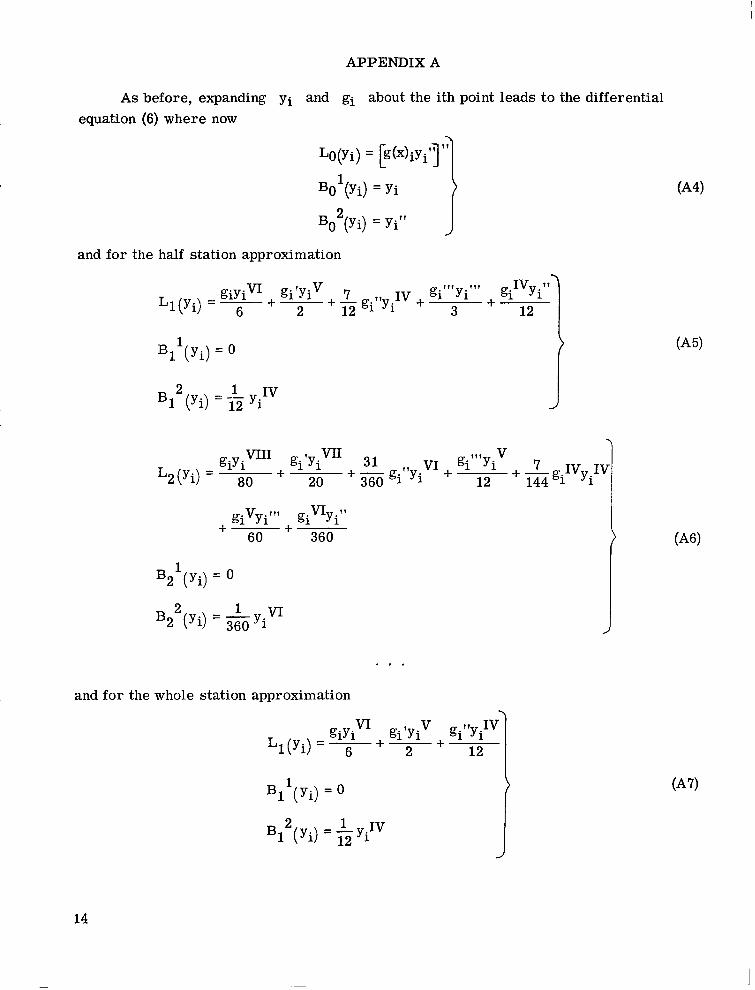
As before, expanding yi and gi about the ith point leads to the differential equation (6) where now

a

J

I 60 ' 360

. . . and for the whole station approximation

giyiVI gilyiv giflYiIV '1 ( Y i ) = 7+ -2 + 12

14

APPENDIX A

. . . If solutions to equations (6) and (7),together with equations (A4) and either equa­

tions (A5), (A6), . . ., or equations (A7), (A8), . . ., are again taken in the form of equa­tion (8 ) , the series of simpler equations (ll),(12), and (13) are again obtained (with p.1 = 1). Since the beam equation is fourth order rather than second, the boundary con­dition of zero bending moment leads to specification of B12 and B22 .

Results have been obtained for

g(x) = xn (n = 2, 3, 4)

(1 5 x 5 2)

for both the half station and whole station approximations of the derivatives. The e r r o r te rms for both deflections and curvatures a r e shown in figure 2 for g(x) = x3 corre­sponding to a linearly tapered beam. An overall measure of the relative e r r o r in the half and whole station approximations is given in figure 3 for all three examples. The analytical e r r o r results for both deflection and curvature also agree with numerical e r r o r calculations within 1 percent for h less than about 0.1.

15

APPENDIX B

CIRCULAR PLATE

Clamped Circular Plate Under Uniform Load

As another example of a second-order equation, consider the axisymmetric bending behavior of a clamped circular plate of radius 1.0 subjected to a uniformly distributed load of magnitude 2. If the plate has constant thickness and appropriate nondimensional variables a r e used, its behavior is governed by a second-order differential equation of

the form t

[;(xQ)j = -x (B1)

where x is the radial distance from the center and where @ represents the slope of the plate. For a clamped plate the boundary conditions a r e @I = 0 at x = 0 and x = 1.

The two finite difference patterns for equation (Bl) a r e as follows:

For the half station approximation,

032) i+

and for the whole station approximation,

The differential operators LO, L1, and L2 in equation (6) a r e given by

BO(Gi) = G i J For the half station approximation,

16

I

APPENDIX B

\

B2 (@i)= 0

and for the whole station approximation,

Results for the average principal e r r o r te rms in the slope and in the numerically obtained second derivative obtained by using the previously described technique a r e presented in figure 3.

Simply Supported Annular Plate Under Uniform Load

The axisymmetric bending behavior of a circular plate is also governed by the fol­lowing fourth-order equation:

where y represents the deflection of the plate. Results are obtained for a clamped plate annulus having an internal radius of 1 and an external radius of 2 and subjected to a uniformly distributed load of magnitude 1. The boundary conditions are y = 0 and y" = 0 at x = 1 and x = 2, respectively.

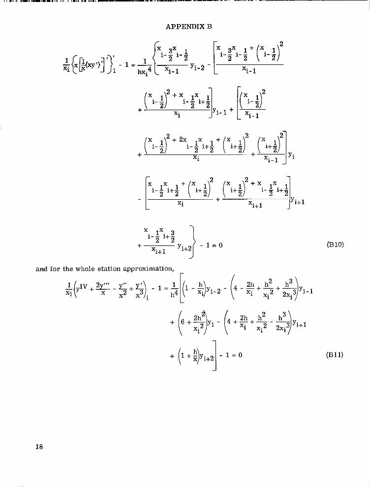
The finite difference approximations to equation (B9) follow, and the results for the average finite difference e r r o r are given in figure 3. For the half station approxirTation,

17

1 1 1 1 1 1 . 1 1 1 I I1111 I1 1111111111111111111.1111 111 I 111111 IIII 11.1 I,,.., ,11111.111 I.,,,., 1.111 1.1,. I---.. I.._..-.-..... I.. ..,, ,...,,,,,,..-., .,, .,...,.-------.-

I

APPENDIX B

2

Yi- 2

i - -lX 3i+- - l = o 2 2 + x.

1+ 1 Yi+2 J

and for the whole station approximation, F

18

APPENDIX B

The differential operators Lo, L1, and L2 in equation (6) are given by

For the half station approximation, -

and for the whole station approximation,

19

~ ~ - ... .... . ...... .,, , .,........,.,,,,.. , . ......-.. ._

APPENDIX B

yim 13yiM --+Y i L2(yi) = 80+ 960% 360xi2 1920xi

J

20

APPENDIX C

DEFLECTIONS OF A MEMBRANE

As an example of the application of the method to a partial differential equation, consider a square membrane subjected to .aunit sinusoidal loading and supported on all edges. The differential equation governing the membrane can be written as

V 2y = sin m m sin n m

y = o (on boundary)I where the length of the side is 1and where y is an appropriate nondimensional deflec­tion. Let equation (Cl) be approximated by finite differences with equal mesh spacing h in both directions. Two finite difference patterns which a r e often used to approximate V 2y are considered in this example. These operators are presented in symbolic form with their Taylor se r ies expansions as follows:

Standard approximation

2Y = V2Y + h (Y-+Yzzzz) + *

L 1 "Refined" approximation

2 4 -20 4 y =V2y + h2(V4y) + . . . 6h2

1 4 1 L -I

where the subscripts denote partial differentiation with respect to the indicated variables. The refined approximation is denoted as such because it utilizes more node points than the standard approximation and for the special case for which the loading is linear (i.e., V4y = 0) has an order of e r r o r of h4 .

The differential operators in equation (6) become

1111 1.1111 I 1 1 1 1 II111111111 111 111 111

APPENDIX C

and for the standard approximation (C2)

Ll(Yi) = Y- +

B1(Yi) = 0

and for the refined approximation (C3)

The finite difference solutions for the deflection at the ith point obtained by the perturbation method give

1 sin mnx sin nnz = .2(m2 + "2)

and the principal e r r o r t e rms for the standard approximation

Y 1 = (1 + $) ~~ sin m m sin nnz

12 I + -( $ and the refined approximation

~ 1 =1sin mnx sin nnz12

Although the refined approximation given by equation (C3)might be considered to be the better approximation, the e r r o r term shows that it is, in fact, l ess accurate for this problem. This result holds for all finite values of m and n; however, for m >> n the e r r o r s in the two methods become essentially the same.

Sample calculations were carried out to obtain actual numerical solutions and to compare them with the exact solution as well as with yi obtained by the perturbation method. Results were obtained for several values of h and m and n for both approximations and substantiate the greater accuracy of the standard approximation for this problem. The results a r e not shown but sample calculations for the dimensionless center deflection with h = 1/4 and m = n = 1 give 0.0533 by the standard approxima­tion and 0.0561 by the refined approximation; the exact answer is 0.0506. With h = 1/4

22

APPENDIX C

agreement was also obtained between the numerical results and the perturbation answers to three digits. This agreement could be improved to 5 digits if the h4 order e r r o r term Y2 was included.

Some practical assessment of the required number of stations to give a certain percentage e r ro r is also possible if equation (8) is written for the deflection as

. . . ) Let the principal e r ro r e be denoted

e = h2 y1- (cii)YO

so that, for example a maximum e r ro r of 10 percent requires that h be chosen such that e < 0.1. For the standard approximation the principal e r ro r is

Since l/m is the length of a displacement Fourier wave, 1 = N is the number of finite difference increments per wave length. Equation (C12) gives

which is fairly insensitive to n/m if m 2 n and which becomes fo r either m >> n or n = m

For example, for a finite difference e r ro r of not more than 10 percent, N = 2.9. This means that approximately three finite difference spaces a r e required within the smallest Fourier wave length in order to obtain a 10-percent accuracy. For a l-percent accuracy, 9.1 spaces are required. Similar developments for the refined approximation give

N =imm

23

APPENDIX C

For m = n, equation (C15) gives N=-7r

J6e (C16)

or N = 4.05 for a 10-percent error and N = 12.8 for a 1-percent error. For m >> n, the error is the same as that for the standard approximation.

24

I

REFERENCES

1. Chuang, K.P.; and Veletsos, A. S.: A Study of Two Approximate Methods of Analyzing Cylindrical Shell Roofs. Struct. Res. Ser. No. 258 (Contract Nonr 1834(03)), Civil Eng. Studies, Univ. of Illinois, Oct. 1962.

2. Cyrus, Nancy Jane; and Fulton, Robert E.: Finite Difference Accuracy in Structural Analysis. Proc. Am. SOC.Civil Engs., J. Struct. Div., vol. 92, no. ST6,Dec. 1966, pp. 459-471.

3. Sepetoski, W.K.;Pearson, C. E.; Dingwell, I. W.; and Adkins, A. W.: A Digital Computer Program for the General Axially Symmetric Thin-Shell Problem. Trans. ASME, Ser. E: J. Appl. Mech., vol. 29, no. 4,Dec. 1962,pp. 655-661.

4.Budianse, Bernard; and Radkowski, Peter P.: Numerical Analysis of Unsymmetrical Bending of Shells of Revolution. AIAA J., vol. 1, no. 8,Aug. 1963,pp. 1833-1842.

5. Newmark, N. M.: Numerical Methods of Analysis of Bars, Plates, and Elastic Bodies. Numerical Methods of Analysis in Engineering, L. E. Grinter, ed. Macmillan Co., 1949,pp. 138-168.

25

Whole station

,.. ,,... , . , ,...

Whole station approximation

*24r -.16

Deflection e r r o r function,

Y1

I I I I 1 I I I I I I

1.o 1.2 1.4 1.6 1.8 2.0 X

--12.0

-Whole station

Curvature -8.0 - approximation er ror function,

-IV ? ?

Y l +- 12 -4.0 ­

- Half station 0’ approximation

I I 1 1 1 1 I I I I

(a) f(x) = i /x3 .

Figure 1.- Fini te difference er ro r in deflection and curvature for a uni formly loaded s t r ing w i th nonuni form tension f(x1.

26

Whole stationDeflection e r r o r function, - approximation 7

y1

Curvature error function,

Whole stationIV -94 approximation Yl" +- 12

approximation .4 .. 1 I I I I I I I I 1

0 .2 .4 .6 .8 1.o X

(b) f(x) = 1 + x3.

Figure 1.- Concluded.

27

Whole station

-Deflection .006 error function,

Yl Half station

1.o 1.2 1.4 1.6 1.8 2.0 X

-.lo Whole station

Curvature -.08 e r ro r function, - .06

X T IV T lY1 + -12 -.04

Half station - .02

0 I 1.0 1.2 1.4 1.6 1.8 2 .o

X

Figure 2.- Finite difference e r ro r in deflection and curvature of a un i formly loaded simply supported beam with nonuni form stiffness g(x) = x3.

28

(a) Solution.

1.2 ­1.0 ­

uyl", whole '6 ­.4­

0 0 & k

9) 9)'.2 - N" N N

0 i 4 - 1

(b) Second derivative.

Figure 3.- Ratio of root-mean-square errors for half and whole station approximations.

“The aeronautical and space activities of the United States shall be conducted 50 as to contribute . . . to the expansion of human knowl­edge of phenomena in the atmosphere and space. The Admifiistration shall provide for the widest practicable and appropriate dissemination of information concerning its activities and the resdts tbereof.”

-NATIONALAERONAUnCS AND SPACE ACT OF 1958

NASA SCIENTIFIC AND TECHNICAL PUBLICATIONS

TECHNICAL REPORTS: Scientific and technical information considered important, complete, and a lasting contribution to existing knowldge.

TECHNICAL NOTES: Information less broad in scope but nevertheless of importance as a contribution to existing knowledge.

TECHNICAL MEMORANDUMS: Information receiving limited distribu­tion because of preliminary data, securityclassification,or other reasons.

CONTRACTOR REPORTS: Scientific and technical information generated under a NASA contract or grant and considered an important contribution to existing knowledge.

TECHNICAL TRANSLATIONS: Information published in a foreign language considered to merit NASA distribution in English.

SPECIAL PUBLICATIONS: Information derived from or of value to NASA activities. Publications include conference proceedings, monographs, data compilations, handbooks, sourcebooks, and special bibliographies.

TECHNOLOGY UTILIZATION PUBLICATIONS: Information on tech­nology used by NASA that may be of particular interest in commercial and other non-aerospace applications. Publications indude Tech Briefs, Technology Utilization Reports and Notes, and Technology Surveys.

Details on the availability of these publications may be obtained from:

SCIENTIFIC AND TECHNICAL INFORMATION DIVISION

NATIONAL AERONAUTICS AND SPACE ADMINISTRATION

Washington, D.C. PO546