finite difference

COMPARISON OF HIGH-ACCURACY FINITE-DIFFERENCE

METHODS FOR LINEAR WAVE PROPAGATION∗

DAVID W. ZINGG†

SIAM J. SCI. COMPUT. c© 2000 Society for Industrial and Applied MathematicsVol. 22, No. 2, pp. 476–502

Abstract. This paper analyzes a number of high-order and optimized finite-difference methodsfor numerically simulating the propagation and scattering of linear waves, such as electromagnetic,acoustic, and elastic waves. The spatial operators analyzed include compact schemes, noncompactschemes, schemes on staggered grids, and schemes which are optimized to produce specific charac-teristics. The time-marching methods include Runge–Kutta methods, Adams–Bashforth methods,and the leapfrog method. In addition, the following fully-discrete finite-difference methods are stud-ied: a one-step implicit scheme with a three-point spatial stencil, a one-step explicit scheme with afive-point spatial stencil, and a two-step explicit scheme with a five-point spatial stencil. For eachmethod, the number of grid points per wavelength required for accurate simulation of wave propaga-tion over large distances is presented. The results provide a clear understanding of the relative meritsof the methods compared, especially the trade-offs associated with the use of optimized methods. Anumerical example is given which shows that the benefits of an optimized scheme can be small if thewaveform has broad spectral content.

Key words. finite-difference methods, wave propagation, electromagnetics, acoustics, Maxwellequations

AMS subject classifications. 65M05, 78A40, 78M20, 76Q05

PII. S1064827599350320

Introduction. Numerical simulation can play an important role in the contextof engineering design and in improving our understanding of complex systems. Thesimulation of wave phenomena, including electromagnetic, elastic, and acoustic waves,is an area of active research. Lighthill [24] and Taflove [40] discuss the prospects forcomputational aeroacoustics and electromagnetics, respectively. The computationalrequirements for accurate simulations of the propagation and scattering of waves canbe high, particularly if the size of the geometry under study is much larger than thewavelength. Consequently, there has been considerable recent effort directed towardsimproving the efficiency of numerical methods for simulating wave phenomena.

In electromagnetics, the most popular approach to the numerical solution of thetime-domain Maxwell equations for numerous applications has been the algorithmof Yee [50], which was named the finite-difference time-domain (FDTD) method byTaflove [41]. This algorithm combines second-order centered differences on a staggeredgrid in space with second-order staggered leapfrog time marching. Its main attributesare its very low cost per grid node and lack of dissipative error. Yee’s method is oftenapplied using Cartesian grids, with a special treatment of curved boundaries [20].Extension to curvilinear grids was carried out by Fusco [11]. Madsen and Ziolowski[28] put the method into a finite-volume framework applicable to unstructured grids.Vinokur and Yarrow [47, 48] developed a related finite-surface method with advantagesat boundaries and grid singularities.

Other methods which have been successfully applied to the time-domain Maxwellequations include the upwind Lax–Wendroff approach used by Shankar, Mohamma-

∗Received by the editors January 28, 1999; accepted for publication(in revised form) December10, 1999; published electronically July 13, 2000.

http://www.siam.org/journals/sisc/22-2/35032.html†University of Toronto Institute for Aerospace Studies, 4925 Dufferin St., Downsview, Ontario,

Canada M3H 5T6 ([email protected]).

476

FINITE-DIFFERENCE METHODS FOR WAVE PROPAGATION 477

dian, and Hall [38], the characteristic-based fractional-step method of Shang [36], andthe finite-element method of Cangellaris, Lin, and Mei [5]. Although all of thesesecond-order methods have been used with a great deal of success, they are efficientonly for geometries of moderate electrical size, on the order of 20 wavelengths orless. For wave propagation over longer distances, the grid resolution requirements ofsecond-order methods can become excessive, leading to impractical CPU and memoryrequirements. This has motivated the development of higher-order methods whichproduce smaller errors for a given grid resolution, such as the extension of Yee’smethod to fourth-order in space [40] and the methods of Liu [25], Shang and Gaitonde[37], Zingg et al. [52, 55, 18, 19], Petropoulos [31], Turkel and Yefet [44], and Young,Gaitonde, and Shang [51], many of which use staggered grids.

In seismology, the need for higher-order methods has been recognized for sometime. Alford, Kelly, and Boore [2], Marfurt [29], Dablain [9], and Sei [34] presenthigher-order algorithms for the elastic wave equation. Similarly, higher-order finite-difference methods have been developed for acoustic applications by Gottlieb andTurkel [13], Cohen and Joly [8], and Davis [10], for example.

It can be advantageous to modify the coefficients of a potentially higher-ordermethod, thereby lowering the order of accuracy, to produce reduced errors over arange of wavenumbers. We refer to such schemes as optimized schemes [52]. Thisapproach was first proposed by Vichnevetsky and De Schutter [45] and later studiedin more detail by Holberg [16] and Lele [23]. Haras and Ta’asan [15] and later Kimand Lee [21] further refined the optimization technique used by Lele. The papers byHolberg and Lele spawned a number of optimized schemes, including those presentedby Hu, Hussaini, and Manthey [17], Lockard, Brentner, and Atkins [27], Sguazzero,Kindelan, and Kamel [35], Tam [42], Tam and Webb [43], Zingg and Lomax [53], andZingg, Lomax, and Jurgens [52, 55]. See Wells and Renaut [49] for a discussion ofseveral of these schemes in the context of computational aeroacoustics.

In addition to the accuracy of the interior differencing scheme, there are severalother important issues in simulating wave phenomena. High-order and optimizedmethods often have a large spatial stencil which cannot be used near boundaries. Thisnecessitates the use of numerical boundary schemes which must be suitably accuraterelative to the interior scheme [14] and stable. These can be difficult to obtain, and thisrepresents a significant obstacle to the use of higher-order methods. Recent progressis reported by Olsson [30] and Carpenter, Gottlieb, and Abarbanel [6, 7]. Zinggand Lomax [54] present a fifth-order numerical boundary scheme which producesa stable scheme in conjunction with sixth-order centered differences. An improvedversion, which is stable for curvilinear grids, is given by Jurgens and Zingg [19].Another important consideration is the boundary condition at the outer boundaryof the domain, which inevitably causes spurious reflection. As a result of recentdevelopments in this area, such as perfectly matched absorbing layers [1, 4, 12, 32, 57],such reflections can be substantially reduced. Consequently, the numerical errorsintroduced by the interior differencing scheme are often dominant, and the choice ofthe interior scheme is critical to the efficient simulation of wave phenomena.

An efficient discretization of a partial differential equation governing a linear wavephenomenon reliably maintains the numerical error below an acceptable threshold,which is problem dependent, at the lowest possible cost. The cost includes processingtime and memory, although development cost can be considered as well. Numericalerrors arise from both the spatial and the temporal discretization. They include bothphase and amplitude errors, which depend on the wavenumber, the grid spacing,

478 DAVID W. ZINGG

the Courant number, and the direction of propagation relative to the grid. Thedependence of the phase speed on the wavenumber results in numerical dispersion[46], while the amplitude error results in numerical dissipation. The dependenceof these errors on the direction of wave propagation relative to the grid leads tonumerical anisotropy. Fourier analysis provides a straightforward means of calculatingthese errors [46, 26]. Although this simplified analysis excludes errors associated withnonuniform grids and boundaries, it is a very useful tool for scheme evaluation anddevelopment. Good performance under the conditions of Fourier analysis, i.e., uniformgrids and periodic boundary conditions, is a necessary condition for good performanceunder more general conditions.

Through Fourier analysis, one can calculate the phase and amplitude error ofa given method as a function of the wavenumber. However, this information canbe difficult to interpret. A more useful approach used by Lockard, Brentner, andAtkins [27] is to plot the grid resolution in terms of grid points per wavelength (PPW)required to maintain global phase and amplitude errors below a specified thresholdas a function of the distance of propagation expressed in terms of the number ofwavelengths traveled. This is not only an excellent metric for scheme developmentand comparison, but it also provides useful information for applying the methods tospecific problems.

In this paper, we study and compare the grid resolution requirements of severalhigh-order and optimized schemes, including spatial discretizations, time-marchingmethods, and combined time-space discretizations. Emphasis is on schemes requiringunder 30 PPW for accurate simulations with propagation distances of up to 200wavelengths. The purpose is twofold. First, the results can aid in the evaluationand application of high-accuracy methods and are especially helpful in clarifying thebehavior of optimized schemes. Second, the framework presented can be used in theassessment of new methods.

Finite-difference schemes compared. In this section, we present the variousfinite-difference schemes in the context of the linear advection equation given by

∂u

∂t+ a

∂u

∂x= 0,(1)

where u is a scalar quantity propagating with speed a, which is real and positive.The schemes under study can be divided into two distinct groups. In the first group,the spatial and temporal discretizations are independent, i.e., a discretization is ap-plied to the spatial derivative to produce a system of ordinary differential equations(ODEs), which is solved numerically using a time-marching method. Hence we firststudy spatial discretizations and time-marching methods separately and later considerspecific combinations. The spatial difference operators are approximations to ∂/∂x.The time-marching methods are presented as applied to a scalar ODE of the form

du

dt= f(u, t).(2)

The second group of methods involves the simultaneous discretization of space andtime; there is no intermediate semidiscrete form. These are presented as applied to(1) itself. The coefficients of all of the schemes studied are given in the appendix.

The methods can also be classified as dissipative or nondissipative. A spatialdiscretization is nondissipative, i.e., produces no amplitude error, if it is skew sym-metric. When combined with certain time-marching methods, such as the leapfrog


method, the resulting full discretization is nondissipative, that is, the amplitude ofthe solution will neither grow nor decay except in the presence of boundaries. Com-bined space-time discretizations can be nondissipative as well. This is generally auseful property in that it is consistent with the physics in preserving certain energynorms. Thus nondissipative schemes are widely used with great success, especiallyin solving the Maxwell equations. However, dissipative schemes can be effective aswell, as long as the numerical dissipation is carefully controlled. For example, in thescheme of Zingg, Lomax, and Jurgens [55], the dissipative error is smaller than thephase error for all wavenumbers. Therefore, any mode for which the numerical dis-sipation is excessive already suffers from excessive phase error. Dissipative schemeshave the advantage that high-frequency spurious waves, arising from boundaries, forexample, are damped [13]. Furthermore, dissipative schemes can, at least in principle,be applied to nonlinear problems.

Spatial difference operators. On a uniform grid with xj = j∆x and uj =u(xj), compact centered-difference schemes of up to tenth order can be representedby the following formula:

β(δxu)j−2 + α(δxu)j−1 + (δxu)j + α(δxu)j+1 + β(δxu)j+2

=1

2∆x

[

c

3(uj+3 − uj−3) +

b

2(uj+2 − uj−2) + a(uj+1 − uj−1)

]

,(3)

where (δxu)j is an approximation to ∂u/∂x at node j. These schemes produce noamplitude error. Noncompact schemes of up to sixth order are obtained with β =α = 0.

Haras and Ta’asan [15] revisited the compact schemes of Lele [23] based on (3) us-ing a more sophisticated optimization procedure. They developed tridiagonal schemes(β = 0) and tridiagonal schemes with a five-point stencil (β = c = 0) as well. In eachcase, Haras and Ta’asan present several methods which result from different param-eters in the optimization procedure. In the comparisons below, we will include onlythose schemes which are best according to our criterion, i.e., those schemes whichrequire the fewest grid points per wavelength for accurate wave propagation over adistance of 200 wavelengths.

The spatial operator of Zingg, Lomax, and Jurgens [52, 55] is noncompact witha seven-point stencil. The operator is divided into a skew-symmetric part given by

(δaxu)j =1

∆x[a3 (uj+3 − uj−3) + a2 (uj+2 − uj−2) + a1 (uj+1 − uj−1)](4)

and a symmetric part given by

(δsxu)j =1

∆x[d3 (uj+3 + uj−3) + d2 (uj+2 + uj−2) + d1 (uj+1 + uj−1) + d0uj ] .(5)

The symmetric part provides dissipation of spurious high-wavenumber components ofthe solution. The magnitude of the dissipative component is chosen such that the am-plitude error produced is less than the phase error. [52, 55] include a maximum-orderscheme and an optimized scheme. The optimized scheme was designed to minimizethe maximum phase and amplitude errors for waves resolved with at least 10 PPW.It is superior for distances of travel of up to 330 wavelengths. Hence we do not con-sider the maximum-order scheme here. Tam and Webb [43] have also developed anoptimized scheme based on the skew-symmetric operator given in (4).

480 DAVID W. ZINGG

Lockard, Brentner, and Atkins [27] present an optimized upwind-biased noncom-pact spatial difference operator based on an eight-point stencil. It can be written inthe form

(δxu)j =1

∆x

3∑

m=−4

amuj+m.(6)

The operator is optimized for waves resolved with at least 7 PPW and providesexcellent accuracy up to about 340 wavelengths of travel. Note that this operatorcan also be written as the sum of a skew-symmetric and a symmetric operator. Anine-point stencil is required for systems of equations with wave speeds of oppositesign.

Differencing schemes on staggered grids are well suited to problems in which thetime derivative of one variable depends on the spatial derivative of the other, and vice-versa. This is the case for the time-domain Maxwell equations or the Euler equationslinearized about a reference state with zero velocity, for example. Centered staggereddifferencing schemes of up to sixth order can be written in the form

(7)

(δxu)j =1

∆x

[

b1(

uj+1/2 − uj−1/2

)

+ b2(

uj+3/2 − uj−3/2

)

+ b3(

uj+5/2 − uj−5/2

)]

.

Time-marching methods. There are many considerations involved in selectinga time-marching method, including efficiency, i.e., accuracy per unit computationaleffort, stability, and memory use. Since wave propagation problems are generallynot particularly stiff, explicit methods are appropriate. Thus the Adams–Bashforthand Runge–Kutta families are suitable candidates. Although other methods, such aspredictor-corrector methods, can be used, we analyze only a few popular options, aswell as some recently introduced methods.

Since a large portion of the computational effort is generally associated withevaluation of the derivative function, one can approximately assess the efficiency of atime-marching method by accounting for the number of derivative function evaluationsper time step. Runge–Kutta methods require one derivative function evaluation perstage. Zingg and Chisholm [56] have shown that for linear ODEs with constantcoefficients, Runge–Kutta methods of up to sixth order can be derived with a numberof stages equal to the order. However, the memory requirements of the methods oforders five and six are high. For nonlinear ODEs and linear ODEs with nonconstantcoefficients, six stages are required for fifth-order accuracy and seven stages for sixth-order accuracy [22].

An alternative approach is to use low-storage multistage methods which are high-order for homogeneous linear ODEs but second-order otherwise [55]. Haras andTa’asan [15] and Zingg, Lomax, and Jurgens [52, 55] present five- and six-stage meth-ods of this type, respectively. For example, when applied to (2), the six-stage methodof Zingg, Lomax, and Jurgens [52, 55] is given by

u(1)n+α1

= un + hα1fn,

u(2)n+α2

= un + hα2f(1)n+α1

,

u(3)n+α3

= un + hα3f(2)n+α2

,(8)

u(4)n+α4

= un + hα4f(3)n+α3

,


u(5)n+α5

= un + hα5f(4)n+α4

,

un+1 = un + hf(5)n+α5

,

where h = ∆t is the time step, tn = nh, un = u(tn), and

f(k)n+α = f(u

(k)n+α, tn + αh).

The five-stage method of [15] is analogous. In their maximum-order form (for ho-mogeneous ODEs), these methods are not stable for pure central (skew-symmetric)differencing in space. Consequently, Haras and Ta’asan modify the coefficients of thefive-stage scheme to produce stability, while Zingg, Lomax, and Jurgens [52, 55] adda dissipative (symmetric) component to their spatial operator, as given in (5).

Adams–Bashforth methods require only one derivative function evaluation pertime step, and thus can be more efficient than Runge–Kutta methods of equal order.Since they are multistep methods, however, they require extra storage. Furthermore,Adams–Bashforth methods of order higher than four have extremely restrictive sta-bility bounds. Thus the time-marching methods we consider here are the fourth-orderAdams–Bashforth method, the low-storage fourth-order Runge–Kutta method for lin-ear ODEs given by Zingg and Chisholm [56], and the low-storage five- and six-stagemethods described above. In terms of stability and Fourier error analysis, the fourth-order Runge–Kutta method of [56] is identical to the classical fourth-order Runge–Kutta method. With respect to memory requirements, the fourth-order Adams–Bashforth method requires five memory locations per dependent variable, while theother methods considered require only two.

A natural choice of time-marching method for use with staggered spatial differ-encing is the second-order staggered leapfrog method, given by

un+1 = un + hfn+1/2.(9)

When used with a nondissipative spatial scheme, as in the FDTD method, the result-ing fully-discrete operator produces no amplitude error. Furthermore, the staggeredleapfrog method generally produces a leading phase error, which can offset the phaselag usually produced by centered spatial differences. At specific Courant numbersand angles of propagation, the perfect-shift property1 can be obtained, leading toexact propagation for all wavenumbers. Although this has little practical significance,fully-discrete methods which possess this property are generally most accurate whenused near the perfect-shift conditions.

Simultaneous space-time discretizations. The scheme of Davis [10] is anondissipative implicit scheme with a three-point spatial stencil. When applied tothe linear advection equation, it is given by

a0un+1j + a1u

n+1j−1 + a2u

n+1j+1 = b0u

nj + b1u

nj−1 + b2u

nj+1(10)

with a0 = b0, a1 = b2, and a2 = b1, where unj = u(xj , tn). Being implicit, this scheme

requires more computational expense than explicit schemes. However, it achievesfourth-order accuracy in time and space with a three-point spatial stencil.

The scheme of Gottlieb and Turkel [13] is an extension of the Lax–Wendroffapproach to fourth-order in space, remaining second-order in time. It is an explicit

1This refers to the situation when the error from the spatial discretization precisely cancels thatfrom the temporal discretization.

482 DAVID W. ZINGG

one-step scheme but requires a five-point stencil. When applied to the linear advectionequation, it is given by

u(1)j = un

j +ah

6∆x(un

j+2 − 8unj+1 + 7un

j ),(11)

un+1j =

1

2(un

j + u(1)j ) +

ah

12∆x(−u

(1)j−2 + 8u

(1)j−1 − 7u

(1)j ).

The two-stage form is motivated by nonlinear problems. This method is dissipativeand has received considerable use in nonlinear problems. The justification for havinga lower order of accuracy in time than in space is based on the idea that the systemis at least mildly stiff. Hence the time-step restriction based on the parasitic modes,i.e., the stability limit, is often much more stringent than that for the driving modes,i.e., the accuracy limit. Note, however, that many wave propagation problems are notstiff at all.

It is straightforward to extend this approach to fourth-order in time withoutincreasing the stencil. For example, one can derive the following dissipative one-stepfourth-order method:

un+1j = un

j − ah(δ(4)x u)nj +

h2a2

2(δ(4)

xx u)nj −h3a3

6(δ(2)

xxxu)nj +h4a4

24(δ(2)

xxxxu)nj ,(12)

where δ(4)x is a fourth-order centered difference approximation to a first derivative,

δ(4)xx is a fourth-order centered difference approximation to a second derivative, δ

(2)xxx

is a second-order centered difference approximation to a third derivative, and δ(2)xxxx

is a second-order centered approximation to a fourth derivative. All of the operatorson the right-hand side require a five-point stencil, as follows:

(δ(4)x u)j =

1

12∆x(uj−2 − 8uj−1 + 8uj+1 − uj+2) ,

(δ(4)xx u)j =

1

12∆x2(−uj−2 + 16uj−1 − 30uj + 16uj+1 − uj+2) ,

(δ(2)xxxu)j =

1

2∆x3(−uj−2 + 2uj−1 − 2uj+1 + uj+2) ,

(δ(2)xxxxu)j =

1

∆x4(uj−2 − 4uj−1 + 6uj − 4uj+1 + uj+2) .(13)

This scheme is quite complicated to apply in multidimensions. Hence we will considera simpler scheme which is fourth-order in time and space, the following nondissipativetwo-step explicit scheme:

un+1j = un−1

j − 2ah(δ(4)x u)nj −

h3a3

3(δ(2)

xxxu)nj ,(14)

where δ(4)x and δ

(2)xxx are given in (13) above. Related methods for the second-order

wave equation are presented by Cohen and Joly [8] and Shubin and Bell [39].

Fourier error analysis. Consider the linear convection equation, (1), on aninfinite domain. A solution initiated by a harmonic function with wavenumber κ is

u(x, t) = f(t)eiκx,(15)

where f(t) satisfies the ODE

df

dt= −iaκf.(16)


If the spatial derivative is approximated by a finite-difference formula, then the ODEbecomes

df

dt= −iaκ∗f,(17)

where κ∗ is the modified wavenumber. For example, the modified wavenumber asso-ciated with the spatial operator given in (3) is obtained from

κ∗∆x =a sin(z) + (b/2) sin(2z) + (c/3) sin(3z)

1 + 2α cos(z) + 2β cos(2z),(18)

where z = κ∆x, i.e., z = 2π/PPW. The numerical phase speed, a∗, is the speedat which a harmonic function propagates numerically. It is related to the modifiedwavenumber by

a∗

a=

κ∗

κ.(19)

The dependence of a∗ on κ introduces numerical dispersion. For the spatial operatorgiven in (4) and (5), the modified wavenumber is obtained from

iκ∗∆x = d0 + 2(d1 cosκ∆x + d2 cos 2κ∆x + d3 cos 3κ∆x)

+ 2i(a1 sinκ∆x + a2 sin 2κ∆x + a3 sin 3κ∆x).(20)

The real part of the modified wavenumber determines the phase (or dispersive) error,while the imaginary part determines the amplitude (or dissipative) error.

The accuracy of a time-marching method can be assessed through the character-istic polynomial of the ODE resulting from application of the time-marching methodto the following ODE:

df

dt= λf.(21)

The accuracy analysis is based on the principal root of the characteristic polynomial,denoted by σ(λh), which is an approximation to eλh. In order to assess the accuracyof time-marching methods for wave propagation, we consider only pure imaginaryvalues of λ, i.e., λ = iω with ω real. The normalized local amplitude and phase errorsare determined from σ(λh), as follows:

era = |σ| − 1,(22)

erp = −φ

ωh+ 1,(23)

where φ = arctan(σi/σr), and σr and σi are the real and imaginary parts of σ.Equation (16) is in the form of (21) with λ = iω = −iaκ. Substituting ω = −aκ into(23), we obtain

erp =φ

zC+ 1,(24)

where σ = σ(−izC), and C = ah/∆x is the Courant number. To analyze a time-marching method in combination with a spatial discretization, σ = σ(−iκ∗∆xC),

484 DAVID W. ZINGG

where κ∗ is the modified wavenumber associated with the spatial operator. For si-multaneous space-time discretizations, the complex amplification factor is calculateddirectly by substituting a solution of the form u(x, t) = σneiκx into the fully discreteoperator [3].

Our criterion for comparing schemes is based on the magnitude of the globalamplitude and phase errors, which are

Era =∣

∣|σ|N − 1∣

∣

=∣

∣

∣|σ|PPWnw/C − 1

∣

∣

∣,(25)

Erp = N |ωh− φ|

= nw

∣

∣

∣

∣

PPWφ

C+ 2π

∣

∣

∣

∣

,(26)

where N = PPWnw/C is the number of time steps and nw is the number of wave-lengths traveled. Using these formulas with an accurate time-marching method anda very small Courant number gives the errors for the spatial operator alone; the timeadvance is effectively exact. In the results section, the various methods are com-pared in terms of the PPW required to keep both global phase and amplitude errorsbelow 0.1 as a function of the number of wavelengths traveled. This error thresh-old is, of course, arbitrary and corresponds to that used by Lockard, Brentner, andAtkins [27]. The relative performance of the methods is similar for other choices, andthus our conclusions are independent of the specific value of the error threshold. Forsome schemes, especially optimized schemes, the error does not increase monotoni-cally with the nondimensional wavenumber z. Hence the error can actually becomelarger as the grid resolution is increased. In such cases, we use the value of PPW forwhich all higher values of PPW also satisfy the error threshold.

Since practical problems involve multidimensional systems of equations, the useof one-dimensional scalar analysis requires some justification. A hyperbolic system ofequations is diagonalizable with real eigenvalues, or wave speeds. These wave speedscan vary significantly. Consequently, the effective Courant number for the differentwaves can also vary significantly. A nonuniform grid further contributes to the vari-ation in the Courant number. For the fastest wave, the Courant number must besufficiently small such that the scheme is both accurate and stable. For the slowerwaves, the Courant number is then much smaller. A scheme which produces pooraccuracy at low Courant numbers is thus inappropriate for such problems. This sit-uation can arise if a scheme relies on cancellation of time and space errors to achievehigh accuracy. For example, several schemes which combine the spatial and temporaldiscretization produce the perfect-shift property at specific Courant numbers. Oftenthis perfect cancellation of temporal and spatial errors is achieved at a Courant num-ber of unity. For such schemes, the error increases as the Courant number is reducedsince the temporal error decreases and no longer cancels the spatial error. Hence itis important to assess schemes over a range of Courant numbers. Note that this isnot an issue with schemes which combine a high-accuracy spatial discretization witha high-accuracy time-marching method. Since such schemes generally do not relyon cancellation to achieve high accuracy, the error does not increase as the Courantnumber is reduced.

The situation is similar in multidimensions. For most spatial discretizations, theerror is largest for waves propagating at 0 or 90 degrees to the grid [46, 23, 53]. The


0 0.1 0.2 0.3 0.4 0.5 0.6–4

–3.5

–3

–2.5

–2

–1.5

–1

–0.5

0

0.5

1x 10

4

ph

ase

sp

ee

d e

rro

r

nondimensional wavenumber

Fig. 1. Phase speed error for the maximum-order (—–) and optimized (- - -) schemes of Zingg,Lomax, and Jurgens [55].

error from the time-marching method is isotropic. Therefore, if there is no cancella-tion of spatial and temporal errors, the one-dimensional analysis is conservative. Incontrast, if a scheme relies on such cancellation, then the error at arbitrary angles ofpropagation can be much higher than that in one dimension. For example, a schemewith the perfect shift property at a Courant number of unity in one dimension canproduce large errors at the same Courant number in multidimensions and can even beunstable. This occurs because the spatial error is anisotropic while the temporal erroris isotropic. Hence they cannot cancel at all angles. Fortunately, this situation can berevealed by a one-dimensional analysis as long as a wide range of Courant numbersis considered. As the Courant number tends to zero, so does the temporal error, andonly the spatial error remains. Hence the one-dimensional analysis at a low Courantnumber can represent the worst case for some schemes, since there is no cancellationof temporal and spatial errors. This is confirmed by the results presented below.

Before proceeding to the results, we briefly discuss the concept of an optimizedscheme, using the schemes of Zingg, Lomax, and Jurgens [55] as an example. Figure 1shows the phase speed error for the maximum-order and optimized spatial discretiza-tions given in [55] for a nondimensional wavenumber z between 0 and π/5, i.e., forwaves resolved with at least 10 PPW. This optimized scheme trades increased errorsat low wavenumbers in return for greatly reduced errors for 0.4 ≤ z ≤ π/5. The ideais to extend the range of wavenumbers for which the scheme is sufficiently accurate.Note that, for the optimized scheme, the error at z = 0.29 (22 PPW) is very close tothat at z = π/5 (10 PPW). Consequently, there is no benefit in increasing the gridresolution from 10 PPW to 22 PPW. If a grid resolution of 10 PPW is insufficientfor a given propagation distance, then greater than 22 PPW will be required. Thisexplains the sudden jumps in the grid resolution requirements of optimized schemeswhich will be seen below.

486 DAVID W. ZINGG

0 20 40 60 80 100 120 140 160 180 2000

10

20

30

40

50

60

70

80

90

100

number of wavelengths of travel

gri

d p

oin

ts p

er

wave

len

gth

Fig. 2. Grid resolution requirements for second-order (—–), fourth-order (- - -), and sixth-order(· · ·) noncompact centered spatial differences.

Results.

Spatial difference operators. In this section, we consider the errors producedby the spatial operators alone. The figures show the PPW required to keep both globalphase and amplitude errors below 0.1 as a function of the number of wavelengthstraveled. Figure 2 shows the grid resolution requirements for second-, fourth-, andsixth-order noncompact centered difference schemes. Since these spatial operators arenondissipative, the grid resolution requirements are determined from the global phaseerror. The requirements of the second-order scheme are clearly excessive. While moreaccurate second-order discretizations are available, such as the FDTD scheme or theupwind leapfrog scheme [33], none of these meets our criterion of 30 PPW for 200wavelengths of travel except under specific conditions.

The PPW requirements for compact centered difference schemes of up to tenthorder are shown in Figure 3. The tenth-order scheme requires the solution of a pen-tadiagonal system of equations. The remaining schemes lead to tridiagonal systems.The compact schemes are considerably more accurate than the noncompact schemesof equivalent order.

We next demonstrate the tradeoffs associated with optimization, using the tridi-agonal five-point operators (β = c = 0) of Haras and Ta’asan as an example. Figure4 shows the behavior of three different optimized schemes given in [15] as well as themaximum-order scheme which can be obtained using this operator, which is sixth-order. Note the presence of sudden jumps in the grid resolution requirements of theoptimized schemes. These are associated with the fact that for an optimized schemethe error does not increase monotonically with increasing wavenumber, as discussedearlier. Their location is dependent on the error threshold used. Reducing the errorallowed moves the jumps to the left. With the present error threshold, the schemedenoted “A” is superior up to a distance of travel of about 60 wavelengths. Scheme B


0 20 40 60 80 100 120 140 160 180 2000

2

4

6

8

10

12

14

16

18

20


gri

d p

oin

ts p

er

wave

len

gth

Fig. 3. Grid resolution requirements for fourth-order (—–), sixth-order (- - -), eighth-order(· · ·), and tenth-order (− · −) compact centered spatial differences.

0 200 400 600 800 10000

2

4

6

8

10

12

14


gri

d p

oin

ts p

er

wave

length

Fig. 4. Grid resolution requirements for the tridiagonal spatial operators with 5-point right-hand stencil of Haras and Ta’asan [15]: scheme A (—–), scheme B (- - -), scheme C (···), sixth-orderscheme (− · −).

is superior for distances up to 250 wavelengths while scheme C is preferable for evenlonger distances. Such behavior is typical of optimized schemes. Aggressive optimiza-tion (as in the case of scheme A) leads to excellent performance for small distances

488 DAVID W. ZINGG

of travel but poor performance for longer distances. In this paper we concentrate ondistances of travel up to 200 wavelengths. Hence we consider only scheme B further.

Figure 5 shows the PPW required by the optimized schemes of Haras and Ta’asanfor distances of travel up to 200 wavelengths. In each case, the best scheme presentedby Haras and Ta’asan for this distance of travel is shown, as discussed above. Thepentadiagonal scheme requires about 3.7 PPW for 200 wavelengths of travel whilethe tridiagonal seven-point scheme requires 4.5 and the tridiagonal five-point schemerequires 5.7. The computational effort is roughly proportional to PPW d+1, whered is the number of dimensions, since the number of grid nodes is proportional toPPW d, and the additional factor of PPW is associated with the decrease in thetime step required to maintain a constant Courant number as PPW is increased, i.e.,N = PPWnw/C. Therefore the increased cost per grid node of the pentadiagonalscheme is not justified. However, the tridiagonal seven-point scheme is more efficientthan the tridiagonal five-point scheme.

The noncompact optimized schemes of Lockard, Brentner, and Atkins [27], Zingg,Lomax, and Jurgens [55], and Tam and Webb [43] are compared with sixth-order cen-tered differences in Figure 6. For the scheme of Lockard, Brentner, and Atkins [27], thePPW requirements are determined by the amplitude error. For the scheme of Zingg,Lomax, and Jurgens [55], the phase and amplitude errors produce roughly equivalentgrid resolution requirements over this distance. Since Tam and Webb’s scheme [43] isnondissipative, its PPW requirements are determined by the phase error. The figureshows that Tam and Webb’s scheme [43] has been optimized for fairly small distancesof travel, leading to excellent performance for less than roughly 14 wavelengths oftravel. The scheme of Lockard, Brentner, and Atkins [27] requires roughly 8 PPW for200 wavelengths of travel while that of Zingg, Lomax, and Jurgens [55] requires over9 PPW.

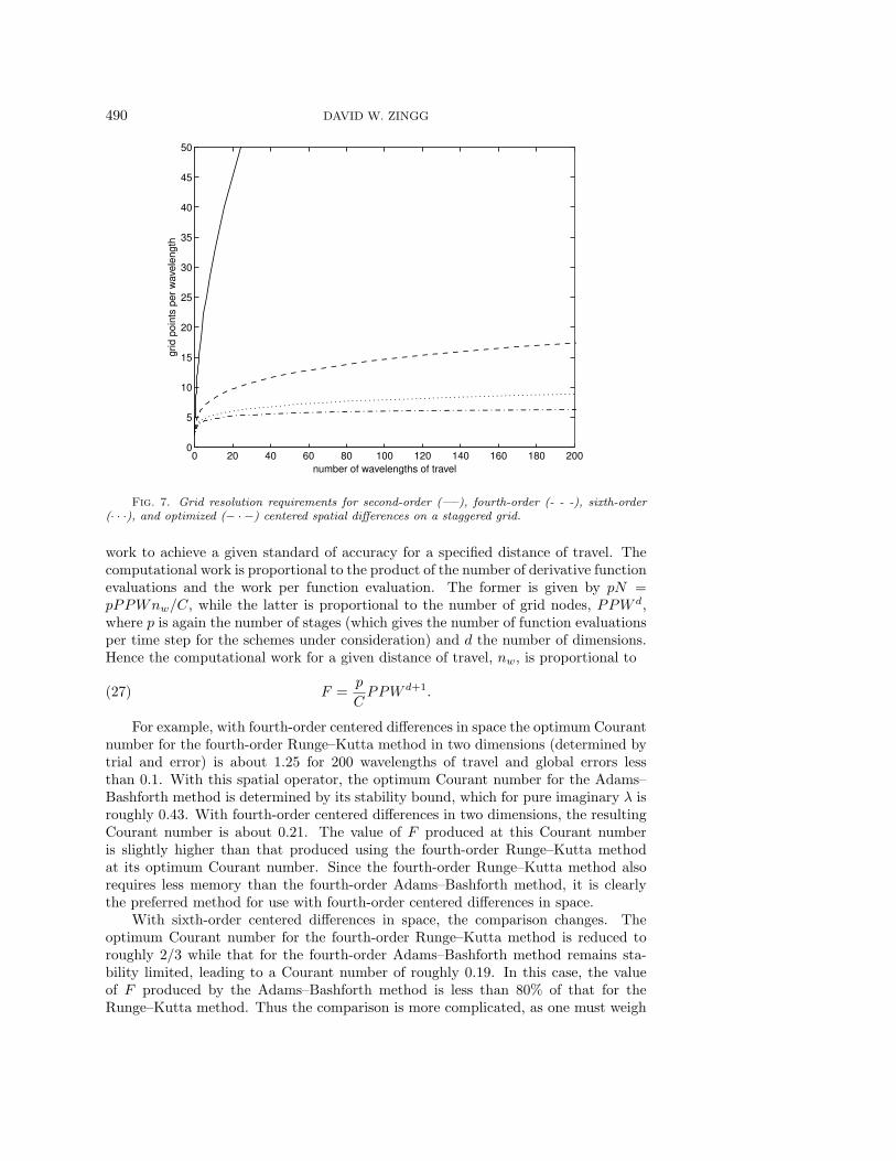
Figure 7 shows the PPW requirements of the staggered spatial operators. Ineach case, the staggered schemes are much more accurate than their nonstaggeredcounterparts of equivalent order. The grid requirements of the second-order schemeare again excessive. However, when used with staggered leapfrog time marching (theFDTD scheme), better results can be obtained. Also shown in Figure 7 is an optimizedscheme with b3 = 103/19200, b2 = −1315/19200, and b1 = 22630/19200, whichproduces excellent performance for up to 200 wavelengths of travel.

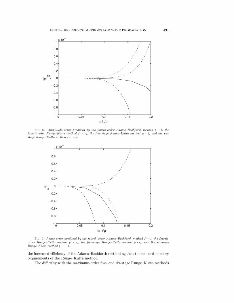
Time-marching methods. Figures 8 and 9 show the amplitude and phase er-rors produced by the four time-marching methods under consideration. The five- andsix-stage methods shown are the maximum-order versions rather than the optimizedmethods, which are discussed in the next subsection. In order to account for thenumber of stages in the Runge–Kutta methods, the errors are plotted versus ωh/p,where p is the number of stages. Hence the errors shown are for approximately equalcomputational effort. Since the time step of a p-stage scheme is thus p times largerthan that of a single-stage scheme, the amplitude error shown is |σ|1/p − 1.

The figures show that the phase errors produced by these methods are largerthan the amplitude errors. Each increase in the order of the Runge–Kutta methodproduces an increase in accuracy even though the extra work has been accounted for.The fourth-order Adams–Bashforth method is much more accurate than the fourth-order Runge–Kutta method per unit cost. It produces the lowest amplitude error ofthe methods considered and phase error comparable to the five-stage Runge–Kuttamethod.

In order to compare time-marching methods properly, one must consider the


0 50 100 150 2000

1

2

3

4

5

6

7

8


gri

d p

oin

ts p

er

wave

length

Fig. 5. Grid resolution requirements for the spatial operators of Haras and Ta’asan [15]: pen-tadiagonal operator with seven-point right-hand stencil (—–), tridiagonal operator with seven-pointright-hand stencil (- - -), tridiagonal operator with five-point right-hand stencil (· · ·).

0 50 100 150 2000

2

4

6

8

10

12

14

16

18

20

number of wavelengths travelled

gri

d p

oin

ts p

er

wave

length

Fig. 6. Grid resolution requirements for the spatial operators of Lockard, Brentner, andAtkins [27] (—–), Zingg, Lomax, and Jurgens [55] (- - -), Tam and Webb [43] (· · ·), and sixth-order centered differences (− · −).

spatial discretization to be used. For each combination of a spatial discretization and atime-marching method, there is a Courant number which minimizes the computational

490 DAVID W. ZINGG

0 20 40 60 80 100 120 140 160 180 2000

5

10

15

20

25

30

35

40

45

50


gri

d p

oin

ts p

er

wave

len

gth

Fig. 7. Grid resolution requirements for second-order (—–), fourth-order (- - -), sixth-order(· · ·), and optimized (− · −) centered spatial differences on a staggered grid.

work to achieve a given standard of accuracy for a specified distance of travel. Thecomputational work is proportional to the product of the number of derivative functionevaluations and the work per function evaluation. The former is given by pN =pPPWnw/C, while the latter is proportional to the number of grid nodes, PPW d,where p is again the number of stages (which gives the number of function evaluationsper time step for the schemes under consideration) and d the number of dimensions.Hence the computational work for a given distance of travel, nw, is proportional to

F =p

CPPW d+1.(27)

For example, with fourth-order centered differences in space the optimum Courantnumber for the fourth-order Runge–Kutta method in two dimensions (determined bytrial and error) is about 1.25 for 200 wavelengths of travel and global errors lessthan 0.1. With this spatial operator, the optimum Courant number for the Adams–Bashforth method is determined by its stability bound, which for pure imaginary λ isroughly 0.43. With fourth-order centered differences in two dimensions, the resultingCourant number is about 0.21. The value of F produced at this Courant numberis slightly higher than that produced using the fourth-order Runge–Kutta methodat its optimum Courant number. Since the fourth-order Runge–Kutta method alsorequires less memory than the fourth-order Adams–Bashforth method, it is clearlythe preferred method for use with fourth-order centered differences in space.

With sixth-order centered differences in space, the comparison changes. Theoptimum Courant number for the fourth-order Runge–Kutta method is reduced toroughly 2/3 while that for the fourth-order Adams–Bashforth method remains sta-bility limited, leading to a Courant number of roughly 0.19. In this case, the valueof F produced by the Adams–Bashforth method is less than 80% of that for theRunge–Kutta method. Thus the comparison is more complicated, as one must weigh


0 0.05 0.1 0.15 0.2-1

-0.8

-0.6

-0.4

-0.2

0

0.2

0.4

0.6

0.8

1x 10

-4

ω h/p

|σ|1/p

1

Fig. 8. Amplitude error produced by the fourth-order Adams–Bashforth method (—–), thefourth-order Runge–Kutta method (- - -), the five-stage Runge–Kutta method (· · ·), and the six-stage Runge–Kutta method (− · −).

0 0.05 0.1 0.15 0.2-1

-0.8

-0.6

-0.4

-0.2

0

0.2

0.4

0.6

0.8

1x 10

-4

ω h/p

erp

Fig. 9. Phase error produced by the fourth-order Adams–Bashforth method (—–), the fourth-order Runge–Kutta method (- - -), the five-stage Runge–Kutta method (· · ·), and the six-stageRunge–Kutta method (− · −).

the increased efficiency of the Adams–Bashforth method against the reduced memoryrequirements of the Runge–Kutta method.

The difficulty with the maximum-order five- and six-stage Runge–Kutta methods

492 DAVID W. ZINGG

0 50 100 150 2000

1

2

3

4

5

6

7

8

9

10


gri

d p

oin

ts p

er

wave

len

gth

Fig. 10. Grid resolution requirements for the spatial and temporal operators of Haras andTa’asan [15] at a Courant number of 0.9: pentadiagonal operator with seven-point right-hand stencil(—–), tridiagonal operator with seven-point right-hand stencil (- - -), tridiagonal operator with five-point right-hand stencil (· · ·); spatial and temporal operators of Zingg, Lomax, and Jurgens [55] ata Courant number of 1 (− · −).

is that they are unstable for pure imaginary λ, as shown in Figure 8. We considerthese schemes further below.

Combined space-time discretizations. Haras and Ta’asan modified the coef-ficients of the five-stage Runge–Kutta method to produce stability for pure imaginaryλ while maintaining second-order accuracy and optimized error behavior. The meth-ods are designed for C = 0.9. Figure 10 shows the grid resolution requirements of thethree spatial operators of Haras and Ta’asan compared in Figure 5 in combinationwith their five-stage time-marching method at a Courant number of 0.9. All threeschemes require between 7 and 8 PPW for 200 wavelengths of travel. The advantageof the more accurate spatial operators has been lost. Either a lower Courant numberor a more accurate time-marching method should be used.

As a result of the dissipation in the spatial operator, the six-stage time-marchingmethod of Zingg, Lomax, and Jurgens [55] is stable up to a Courant number a littlegreater than unity in two dimensions. The grid requirements for the combined space-time discretization at a Courant number of unity are shown in Figure 10. Comparisonwith Figure 6 shows that the time-marching method introduces very little error com-pared to the spatial differencing. Tam and Webb [43] use an optimized four-stepAdams–Bashforth method in conjunction with their spatial operator. It produces lit-tle error for Courant numbers less than about 0.3. In both cases, optimization of thetime-marching method has a much smaller impact than optimization of the spatialoperator.

Figure 11 shows the PPW requirements of the fourth-order staggered spatial dif-ference operator combined with staggered leapfrog time marching. As the Courantnumber is increased from 0.001 to 0.1, the PPW requirements decrease, since the


0 20 40 60 80 100 120 140 160 180 2000

5

10

15

20

25

30


gri

d p

oin

ts p

er

wave

length

Fig. 11. Grid resolution requirements for fourth-order centered differences on a staggered gridcoupled with staggered leapfrog time marching at Courant numbers of 0.2 (—–), 0.1 (- - -), and 0.001(· · ·).

0 50 100 150 2000

5

10

15

20

25

30

35

40

45

50


gri

d p

oin

ts p

er

wave

length

Fig. 12. Grid resolution requirements for the scheme of Davis [10] at Courant numbers of 3(—–), 1.5 (- - -), and 0.01 (· · ·).

error from the time-marching method is of opposite sign to that of the spatial op-erator. However, as the Courant number is further increased, the error from thesecond-order time-marching method begins to dominate. Excellent performance for

494 DAVID W. ZINGG

200 wavelengths of travel is obtained for Courant numbers up to 0.1.

Results for the method of Davis [10] are shown in Figure 12. Since the methodis nondissipative, the PPW requirements are determined from the phase error. Thisscheme is unconditionally stable. For Courant numbers under 1.5, less than 19 PPWare required for 200 wavelengths of travel. While this is quite good, much betterthan many schemes, it is not sufficient to justify the additional computational effortassociated with an implicit scheme.

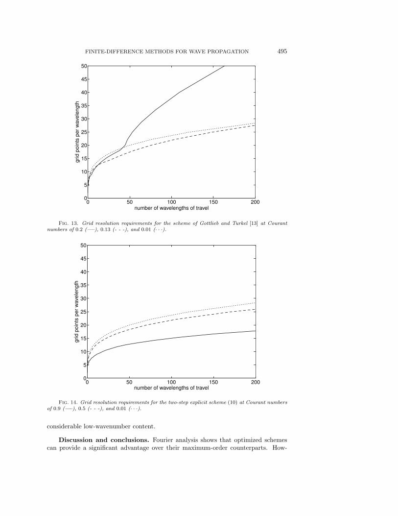
Figure 13 shows the grid resolution requirements for the Gottlieb–Turkel scheme,which is stable up to a Courant number of 2/3 in one dimension. This scheme is veryrobust and has received extensive use in nonlinear applications. Since the method isonly second-order in time, high accuracy is obtained only for Courant numbers lessthan about 0.13. Less than 29 PPW are required to propagate a wave 200 wavelengthswith Courant numbers below this value. Although the cost per grid node is reasonablylow, these PPW requirements are too high for efficient simulation over such distances.

Finally, the grid requirements of the nondissipative two-step explicit scheme, (14),are shown in Figure 14. This scheme is stable up to a Courant number of unity in onedimension. It has the perfect shift property at this Courant number. The phase errorincreases as the Courant number is reduced. Less than 29 PPW are required for allstable Courant numbers. Since it provides reasonably low error at Courant numbersup to unity, this scheme has a very low cost per grid node, substantially lower thanthe Gottlieb–Turkel scheme. However, the PPW requirements are again much higherthan some of the other schemes considered.

A numerical example. In this section, we present a numerical simulation ofthe propagation and reflection of an electromagnetic wave which demonstrates the ap-plicability of the previous analysis in multidimensional cases using nonuniform curvi-linear grids. Further details, including the treatment of the boundary conditions,are available in [19]. The governing equations are the transverse magnetic set of thetwo-dimensional time-domain Maxwell equations. The simulation consists of a pulsedplane wave incident on a perfectly-conducting cylinder. A grid containing 5,400 nodesis shown in Figure 15. Figure 16 shows a snapshot of the electric field intensity com-puted on a grid with 21,600 nodes using the maximum-order version of the method ofZingg, Lomax, and Jurgens [52, 55]. The dashed contours indicate negative values ofthe electric field intensity. This solution is visually indistinguishable from that com-puted using the same method on a grid with 16 times as many nodes, which is usedas a baseline to estimate numerical errors. The reflected wave has not yet reached theouter boundary, so spurious reflections are not an issue.

Figures 17 and 18 show the L2 norm of the numerical error versus the num-ber of grid nodes and the CPU effort, respectively. Four methods are included,the maximum-order (MO) and optimized (O10) schemes of Zingg, Lomax, and Jur-gens [52, 55], as well as second- (C2) and fourth-order (C4) centered differences. Thesecond- and fourth-order difference schemes are combined with fourth-order Runge–Kutta time marching and include a very small amount of artificial dissipation forstability. These figures show that the higher-order and optimized methods lead tosubstantial reductions in both memory and CPU time. The relative grid resolutionrequirements of the methods are consistent with the predictions obtained from Fourieranalysis. Furthermore, the results show that the increased cost per grid node of thehigher-order methods is insignificant compared to the reduction in grid resolution re-quired. The benefits of the optimized scheme over the maximum-order scheme arefairly modest due to the nature of the waveform, which is a Gaussian and thus has


0 50 100 150 2000

5

10

15

20

25

30

35

40

45

50


gri

d p

oin

ts p

er

wave

length

Fig. 13. Grid resolution requirements for the scheme of Gottlieb and Turkel [13] at Courantnumbers of 0.2 (—–), 0.13 (- - -), and 0.01 (· · ·).

0 50 100 150 2000

5

10

15

20

25

30

35

40

45

50


gri

d p

oin

ts p

er

wave

len

gth

Fig. 14. Grid resolution requirements for the two-step explicit scheme (10) at Courant numbersof 0.9 (—–), 0.5 (- - -), and 0.01 (· · ·).

considerable low-wavenumber content.

Discussion and conclusions. Fourier analysis shows that optimized schemescan provide a significant advantage over their maximum-order counterparts. How-

496 DAVID W. ZINGG

-5 -4 -3 -2 -1 0 1 2 3 4 5

Fig. 15. Grid for the perfectly-conducting cylinder.

-5 -4 -3 -2 -1 0 1 2 3 4 5

Fig. 16. Computed contours of electric field intensity.


104

10510

-4

10-3

10-2

10-1

Number of Nodes

Err

or

C2

C4

MO

O10

Fig. 17. Error in the electric field intensity as a function of the number of grid nodes.

100

101

10210

-4

10-3

10-2

10-1

CPU Time (billions of cycles)

Err

or

C2

C4

MO

O10

Fig. 18. Error in the electric field intensity as a function of the CPU time.

ever, if optimized too aggressively, they perform poorly for longer distances of travel.Furthermore, if a waveform has significant low wavenumber content, as in the case ofa Gaussian pulse, the benefits of an optimized scheme can be minimal, and maximum-order schemes can even be superior. The spatial operators of Haras and Ta’asan [15],Lockard, Brentner, and Atkins [27], and Zingg, Lomax, and Jurgens [52, 55] all provideadequate accuracy for 200 wavelengths of travel. The selection of a time-marchingmethod is not quite as critical, since the computational work varies linearly with thetime-step size. Consequently, the cost of reducing the time step is much less than the

498 DAVID W. ZINGG

cost of reducing the PPW, and, furthermore, has no memory implications. Adams–Bashforth and low-storage Runge–Kutta methods can be used, with the latter oftenpreferable because of their reduced memory requirements.

For appropriate problems, such as those involving electromagnetic waves or acous-tic waves in a quiescent medium, staggered spatial schemes perform very well. Thesecan be combined with either a high-order time-marching method or the staggeredleapfrog method. In the latter case, a low Courant number should be used. For largepropagation distances, higher-order time-marching methods are more efficient.

The grid requirements of the explicit fourth-order methods involving simultaneousspace-time discretization are reasonably low considering the low cost of these schemes,especially the two-step explicit scheme. This suggests that sixth-order and optimizedextensions of these schemes are worthy of investigation.

Based on the results presented, it is clear that high-order and optimized finite-difference methods will play an important role in the simulation of high-frequencylinear wave phenomena. Several of the methods studied have the potential to sub-stantially reduce the computational requirements for accurate simulations, includingboth CPU time and memory. The choice of an optimization strategy can be correlatedwith a specific distance of propagation. Among the various optimized schemes of Ha-ras and Ta’asan, for example, specific choices can be made if the propagation distancecan be estimated. This suggests the use of optimized schemes which are specificallytailored to the spectral content and distance of propagation of a given simulation.In addition to providing a useful reference for scheme evaluation and comparison,our results can be used as a basis for selecting an appropriate grid resolution whenapplying these schemes.

Appendix. The following are the coefficients of the finite-difference schemesstudied. The number of significant figures given is based on the number given in thecited references.

The spatial operator of Haras and Ta’asan is given in (3). The schemes shown inFigure 4 have β = c = 0. The remaining coefficients are

Scheme A:

α = 0.3534620453,

a = 1.566965775,

b = 0.1399583152;

Scheme B:

α = 0.3461890571,

a = 1.5633098070,

b = 0.1290683071;

Scheme C:

α = 0.3427812069,

a = 1.5614141543,

b = 0.124148259.

In Figure 5, the pentadiagonal seven-point scheme has

α = 0.5801818925,


β = 0.0877284887,

a = 1.3058941939,

b = 0.9975884963,

c = 0.0323380724.

The tridiagonal seven-point scheme has

α = 0.3904091387,

β = 0,

a = 1.5638887738,

b = 0.2348222711,

c = −0.0178927675.

The tridiagonal five-point operator is scheme B above.In Figure 6, the scheme of Lockard, Brentner, and Atkins is the average of two

schemes with the following coefficients, as defined in (6):

a−4 = 0.0207860419,

a−3 = −0.1500704734,

a−2 = 0.5234309723,

a−1 = −1.34207332539,

a0 = 0.574548248808,

a1 = 0.4090357053658,

a2 = −0.035657169508

and

a0 = 0,a1 = −a−1 = 0.763289242273,a2 = −a−2 = −0.160631393818,a3 = −a−3 = 0.019324515121.

The optimized scheme of Zingg, Lomax, and Jurgens [52, 55] is given by (4) and (5)with the following coefficients:

a1 = 0.75996126,

a2 = −0.15812197,

a3 = 0.018760895,

d0 = 0.1,

d1 = −0.076384622,

d2 = 0.032289620,

d3 = −0.0059049989.

Tam and Webb’s scheme is obtained from (4) with (coefficients are from [42])

a1 = 0.770882380518,

a2 = −0.166705904415,

a3 = 0.0208431427703.

500 DAVID W. ZINGG

The five-stage Runge–Kutta method shown in Figures 8 and 9 has the followingcharacteristic polynomial:

σ(λh) = 1 + λh +(λh)2

2+

(λh)3

6+

(λh)4

24+

(λh)5

120.

The six-stage method is obtained from (8) with α5 = 1/2, α4 = 1/3, α3 = 1/4,α2 = 1/5, α1 = 1/6, leading to the following characteristic polynomial:

σ(λh) = 1 + λh +(λh)2

2+

(λh)3

6+

(λh)4

24+

(λh)5

120+

(λh)6

720.

The characteristic polynomial of the optimized five-stage Runge–Kutta methodof Haras and Ta’asan used in Figure 10 is

σ(λh) = 1 + λh +(λh)2

2+ 0.166407(λh)3 + 0.0409525(λh)4 + 0.0074510(λh)5.

The optimized temporal operator of Zingg, Lomax, and Jurgens [52, 55] is obtainedfrom (8) with the following coefficients:

α1 = 0.168850,

α2 = 0.197348,

α3 = 0.250038,

α4 = 0.333306,

α5 = 0.5.

The resulting characteristic polynomial is

σ(λh) = 1 + λh +(λh)2

2+ 0.16665295(λh)3 + 0.041669557(λh)4

+ 0.0082233848(λh)5 + 0.0013885169(λh)6.

The scheme of Davis is obtained from (10) with

a0 = b0 = −2(C − 2)(C + 2),a1 = b2 = (C − 1)(C − 2),a2 = b1 = (C + 1)(C + 2),

where C = ah/∆x is the Courant number.

REFERENCES

[1] S. Abarbanel, D. Gottlieb, and J.S. Hesthaven, Well-posed perfectly matched layers foradvective acoustics, J. Comput. Phys., 154 (1999), pp. 266–283.

[2] R.M. Alford, K.R. Kelly, and D.M. Boore, Accuracy of finite-difference modelling of theacoustic wave equation, Geophysics, 39 (1974), pp. 834–842.

[3] D.A. Anderson, J.C. Tannehill, and R.H. Pletcher, Computational Fluid Mechanics andHeat Transfer, McGraw-Hill, New York, 1984, p. 73.

[4] J.-P. Berenger, A perfectly matched layer for the absorption of electromagnetic waves, J.Comput. Phys., 114 (1994), pp. 185–200.

[5] A.C. Cangellaris, C.-C. Lin., and K.K. Mei, Point-matched time-domain finite elementmethods for electromagnetic radiation and scattering, IEEE Trans. Antennas and Propa-gation, 35 (1987), pp. 1160–1173.


[6] M.H. Carpenter, D. Gottlieb, and S. Abarbanel, Stable and accurate boundary treatmentsfor compact, high-order finite-difference schemes, Appl. Numer. Math., 12 (1993), pp. 55–87.

[7] M.H. Carpenter, D. Gottlieb, and S. Abarbanel, Time-stable boundary conditions forfinite-difference schemes solving hyperbolic systems: Methodology and application to high-order compact schemes, J. Comput. Phys., 111 (1994), pp. 220–236.

[8] G. Cohen and P. Joly, Fourth order schemes for the heterogeneous acoustics equation, Com-put. Methods Appl. Mech. Engrg., 80 (1990), pp. 397–407.

[9] M.A. Dablain, The application of high-order differencing to the scalar wave equation, Geo-physics, 51 (1986), pp. 54–66.

[10] S. Davis, Low-dispersion finite difference methods for acoustic waves in a pipe, J. Acoust. Soc.Amer., 90 (1991), pp. 2775–2781.

[11] M. Fusco, FDTD algorithm in curvilinear coordinates, IEEE Trans. Antennas and Propaga-tion, 38 (1990), pp. 78–89.

[12] S.D. Gedney, An anisotropic perfectly matched layer absorbing medium for the truncation ofFDTD lattices, IEEE Trans. Antennas and Propagation, 44 (1996), pp. 1630–1639.

[13] D. Gottlieb and E. Turkel, Dissipative two-four methods for time-dependent problems,Math. Comp., 30 (1976), pp. 703–723.

[14] B. Gustafsson, The convergence rate for difference approximations to mixed initial boundaryvalue problems, Math. Comp., 29 (1975), pp. 396–406.

[15] Z. Haras and S. Ta’asan, Finite-difference schemes for long-time integration, J. Comput.Phys., 114 (1994), pp. 265–279.

[16] O. Holberg, Computational aspects of the choice of operator and sampling interval for numer-ical differentiation in large-scale simulation of wave phenomena, Geophysical Prospecting,35 (1987), pp. 629–655.

[17] F.Q. Hu, M.Y. Hussaini, and J.L. Manthey, Low-dissipation and low-dispersion Runge-Kuttaschemes for computational acoustics, J. Comput. Phys., 124 (1996), pp. 177–191.

[18] H.M. Jurgens and D.W. Zingg, Implementation of a high-accuracy finite-difference schemefor linear wave phenomena, Proceedings of the Third International Conference on Spectraland High Order Methods, Houston, TX, Houston J. Math. (1995).

[19] H.M. Jurgens and D.W. Zingg, Numerical solution of the time-domain Maxwell equationsusing high-accuracy finite-difference methods, SIAM J. Sci. Comput., to appear.

[20] T.G. Jurgens, A. Taflove, K.R. Umashankar, and T.G. Moore, Finite-difference time-domain modeling of curved surfaces, IEEE Trans. Antennas and Propagation, 40 (1992),pp. 357–366.

[21] J.W. Kim and D.J. Lee, Optimized compact finite difference schemes with maximum resolu-tion, AIAA J., 34 (1996), pp. 887–893.

[22] J.D. Lambert, Computational Methods in Ordinary Differential Equations, Wiley, New York,1973.

[23] S.K. Lele, Compact finite difference schemes with spectral-like resolution, J. Comput. Phys.,103 (1992), pp. 16–42.

[24] J. Lighthill, The final panel discussion, in Computational Aeroacoustics, J.C. Hardin andM.Y. Hussaini, eds., Springer-Verlag, New York, 1993, pp. 499–513.

[25] Y. Liu, A generalized finite-volume algorithm for solving the Maxwell equations on arbitrarygrids, Conference Proceedings of the 10th Annual Review of Progress in Applied Compu-tational Electromagnetics, 1994, pp. 487–494.

[26] Y. Liu, Fourier analysis of numerical algorithms for the Maxwell equations, J. Comput. Phys.,124 (1996), pp. 396–416.

[27] D.P. Lockard, K.S. Brentner, and H.L. Atkins, High accuracy algorithms for computa-tional aeroacoustics, AIAA J., 33 (1994), pp. 246–251.

[28] N.K. Madsen and R.W. Ziolowski, A three-dimensional modified finite volume technique forMaxwell’s equations, Electromagnetics, 10 (1990), pp. 147–161.

[29] K.J. Marfurt, Accuracy of finite-difference and finite-element modeling of the scalar andelastic wave equations, Geophysics, 49 (1984), pp. 533–549.

[30] P. Olsson, Summation by parts, projections, and stability I, Math. Comp., 64 (1995), pp. 1035–1065.

[31] P.G. Petropoulos, Phase error control for FD-TD methods of second and fourth order accu-racy, IEEE Trans. Antennas and Propagation, 42 (1994), pp. 859–862.

[32] P.G. Petropoulos, L. Zhao, and A.C. Cangellaris, A reflectionless sponge layer absorbingboundary condition for the solution of Maxwell’s equations with high-order staggered finitedifference schemes, J. Comput. Phys., 139 (1998), pp. 184–208.

502 DAVID W. ZINGG

[33] P.L. Roe, Linear bicharacteristic schemes without dissipation, SIAM J. Sci. Comput., 19(1998), pp. 1405–1427.

[34] A. Sei, A family of numerical schemes for the computation of elastic waves, SIAM J. Sci.Comput., 16 (1995), pp. 898–916.

[35] P. Sguazzero, M. Kindelan, and A. Kamel, Dispersion-bounded numerical integration ofthe elastodynamic equations with cost-effective staggered schemes, Comput. Methods Appl.Mech. Engrg., 80 (1990), pp. 165–172.

[36] J.S. Shang, A fractional-step method for the time domain Maxwell equations, J. Comput.Phys., 118 (1995), pp. 109–119.

[37] J.S. Shang and D. Gaitonde, On High Resolution Schemes for Time-Dependent MaxwellEquations, AIAA Paper 96-0832, 1996.

[38] V. Shankar, A.H. Mohammadian, and W.F. Hall, A time-domain finite-volume treatmentfor the Maxwell equations, Electromagnetics, 10 (1990), pp. 127–145.

[39] G.R. Shubin and J.B. Bell, A modified equation approach to constructing fourth order meth-ods for acoustic wave propagation, SIAM J. Sci. Statist. Comput., 8 (1987), pp. 135–151.

[40] A. Taflove, Computational Electrodynamics: The Finite-Difference Time-Domain Method,Artech House, Boston, 1995.

[41] A. Taflove, Application of the finite difference time-domain method to sinusoidal steady-state electromagnetic penetration problems, IEEE Trans. Electromagnetic Compatibility,22 (1980), pp. 191–202.

[42] C.K.W. Tam, Computational aeroacoustics: Issues and methods, AIAA J., 33 (1995), pp. 1788–1796.

[43] C.K.W. Tam and J.C. Webb, Dispersion-relation-preserving finite difference schemes for com-putational acoustics, J. Comput. Phys., 107 (1993), pp. 262–281.

[44] E. Turkel and A. Yefet, Fourth order method for Maxwell equations on a staggered mesh,IEEE Antennas and Propagation Society International Symposium 1997 Digest, 4 (1997),pp. 2156–2159.

[45] R. Vichnevetsky and F. De Schutter, A Frequency Analysis of Finite Difference and Finite-Element Methods for Initial Value Problems, in Advances in Computer Methods for Par-tial Differential Equations, R. Vichnevetsky, ed., AICA/IMACS, Rutgers University, NewBrunswick, NJ, 1975, pp. 46–52.

[46] R. Vichnevetsky and J.B. Bowles, Fourier Analysis of Numerical Approximations of Hy-perbolic Equations, SIAM Stud. Appl. Math. 5, SIAM, Philadelphia, 1982.

[47] M. Vinokur and M. Yarrow, Finite-Surface Method for the Maxwell Equations in GeneralizedCoordinates, AIAA Paper 93-0463, 1993.

[48] M. Vinokur and M. Yarrow, Finite-Surface Method for the Maxwell Equations with CornerSingularities, AIAA Paper 94-0233, 1994.

[49] V.L. Wells and R.A. Renaut, Computing aerodynamically generated noise, Annu. Rev. FluidMech., 29 (1997), pp. 161–199.

[50] K.S. Yee, Numerical solution of initial boundary value problems involving Maxwell’s equationsin isotropic media, IEEE Trans. Antennas and Propagation, 14 (1966), pp. 302–307.

[51] J.L. Young, D. Gaitonde, and J.S. Shang, Toward the construction of a fourth-order dif-ference scheme for transient EM wave simulation: Staggered grid approach, IEEE Trans.Antennas and Propagation, 45 (1997), pp. 1573–1580.

[52] D.W. Zingg, H. Lomax, and H.M. Jurgens, An Optimized Finite-Difference Scheme forWave Propagation Problems, AIAA Paper 93-0459, 1993.

[53] D.W. Zingg and H. Lomax, Finite-difference schemes on regular triangular grids, J. Comput.Phys., 108 (1993), pp. 306–313.

[54] D.W. Zingg and H. Lomax, On the eigensystems associated with numerical boundary schemesfor hyperbolic equations, in Numerical Methods for Fluid Dynamics, M.J. Baines and K.W.Morton, eds., Clarendon Press, Oxford, UK, 1993, pp. 471–480.

[55] D.W. Zingg, H. Lomax, and H.M. Jurgens, High-accuracy finite-difference schemes for linearwave propagation, SIAM J. Sci. Comput., 17 (1996), pp. 328–346.

[56] D.W. Zingg, and T.T. Chisholm, Runge-Kutta methods for linear ordinary differential equa-tions, Appl. Numer. Math., 31 (1999), pp. 227–238.

[57] R.W. Ziolkowski, Time-derivative Lorentz-material model based absorbing boundary condi-tions, IEEE Trans. Antennas and Propagation, 45 (1997), pp. 1530–1535.

finite difference

Documents