Accuracy-Aware Aquatic Diffusion Process Profiling UsingRobotic Sensor Networks

Yu Wang∗, Rui Tan∗, Guoliang Xing∗, Jianxun Wang†, and Xiaobo Tan†

∗Department of Computer Science and Engineering, Michigan State University, USA†Department of Electrical and Computer Engineering, Michigan State University, USA

wangyu3, tanrui, glxing, wangji19, xbtan@msu.edu

ABSTRACT

Water resources and aquatic ecosystems are facing increas-ing threats from climate change, improper waste disposal,and oil spill incidents. It is of great interest to deploy mo-bile sensors to detect and monitor certain diffusion processes(e.g., chemical pollutants) that are harmful to aquatic en-vironments. In this paper, we propose an accuracy-awarediffusion process profiling approach using smart aquatic mo-bile sensors such as robotic fish. In our approach, the robot-ic sensors collaboratively profile the characteristics of a d-iffusion process including source location, discharged sub-stance amount, and its evolution over time. In particular,the robotic sensors reposition themselves to progressivelyimprove the profiling accuracy. We formulate a novel move-ment scheduling problem that aims to maximize the profil-ing accuracy subject to limited sensor mobility and energybudget. We develop an efficient greedy algorithm and a morecomplex near-optimal radial algorithm to solve the problem.We conduct extensive simulations based on real data tracesof robotic fish movement and wireless communication. Theresults show that our approach can accurately profile dy-namic diffusion processes under tight energy budgets. More-over, a preliminary evaluation based on the implementationon TelosB motes validates the feasibility of deploying ourmovement scheduling algorithms on mote-class robotic sen-sor platforms.

Categories and Subject Descriptors

C.3 [Special-purpose and Application-based System-s]: Signal processing systems; C.4 [Performance of Sys-tems]: Measurement techniques, modeling techniques; G.1.6[Numerical Analysis]: Optimization—Constrained opti-mization, gradient methods

Keywords

Robotic sensor networks, diffusion process, movement schedul-ing

Permission to make digital or hard copies of all or part of this work forpersonal or classroom use is granted without fee provided that copies arenot made or distributed for profit or commercial advantage and that copiesbear this notice and the full citation on the first page. To copy otherwise, torepublish, to post on servers or to redistribute to lists, requires prior specificpermission and/or a fee.IPSN’12, April 16–20, 2012, Beijing, China.Copyright 2012 ACM 978-1-4503-1227-1/12/04 ...$10.00.

(a) (b)

Figure 1: Prototypes of autonomous robotic fish de-veloped by the Smart Microsystems Laboratory atMichigan State University [26].

1. INTRODUCTIONWater resources and aquatic ecosystems have been facing

various physical, chemical, and biological threats from cli-mate change, industrial pollution, and improper waste dis-posal. For instance, the last four decades witnessed morethan a dozen major oil spills with each releasing more than30 million gallons of oil [1]. Other harmful diffusion process-es like chemical or radiation leaks could also have disastrousimpact on public health and ecosystem sustainability. Whensuch a crisis arises, an immediate requirement is to profilethe characteristics of the diffusion process, including the lo-cation of source, the amount of discharged substance, andhow rapidly it spreads in space and evolves over time.

Manual sampling, via boat/ship or with handhold devices,is still a common practice in the monitoring of aquatic diffu-sion processes. This approach is labor-intensive and difficultto adapt to the dynamic evolution of diffusion. An alterna-tive is in situ sensing with fixed or buoyed/moored sensors[20]. However, since buoyed sensors cannot move around, itcould take a prohibitively large number of them to capturespatially inhomogeneous information. The past couple ofdecades have seen significant progress in developing robotictechnologies for aquatic sensing. Autonomous underwatervehicles (AUVs) [10] and sea gliders [9] are notable exam-ples of such technologies. However, because of their highcost (over 50,000 U.S. dollars per unit [21]), weight (over100 pounds), and size (1-2meters long), it is difficult to de-ploy many AUVs or sea gliders for temporally and spatiallyresolved measurement of diffusion processes.

Recent advances in computing, communication, sensing,and actuation technologies have made it possible to createuntethered robotic fish with onboard power, control, naviga-tion, wireless communication, and sensing modules, whichturn these robots into mobile sensing platforms in aquat-

ic environments. Fig. 1(a) shows a prototype of robotic fishswimming in an inland lake. Fig. 1(b) shows the close-up of arobotic fish prototype, equipped with GPS, Zigbee antenna,and a dissolved oxygen (DO) sensor. Due to the low man-ufacturing cost, these platforms can be massively deployedto form a mobile sensor network that monitors harmful d-iffusion processes, providing significantly higher spatial andtemporal sensing resolution than existing monitoring meth-ods. Moreover, a school of robotic fish can coordinate theirsensing and movements through wireless communication en-abled by the onboard Zigbee radio, to adapt to the dynamicsof evolving diffusion processes.Despite the aforementioned advantages, low-cost mobile

sensing platforms like robotic fish introduce several chal-lenges for aquatic sensing. First, due to the constraints onsize and energy, they are typically equipped with low-endsensors whose measurements are subject to significant biasesand noises. They must efficiently collaborate in data pro-cessing to achieve satisfactory accuracy in diffusion profiling.Second, practical aquatic mobile platforms are only capableof relatively low-speed movements. Hence the movementsof sensors must be efficiently scheduled to achieve real-timeprofiling of the diffusion processes that may evolve rapidlyover time. Third, given the high power consumption of loco-motion, the distance that mobile sensors move in a profilingprocess should be minimized to extend the network lifetime.We make the following major contributions in this paper:

• We propose a novel accuracy-aware approach for aquat-ic diffusion profiling based on robotic sensor networks.Our approach leverages the mobility of robotic sensorsto iteratively profile the spatiotemporally evolving d-iffusion process.

• We derive the analytical profiling accuracy of our ap-proach based on the Cramer-Rao bound (CRB). Thenwe formulate a movement scheduling problem for aquat-ic diffusion profiling, in which the profiling accuracyis maximized under the constraints on sensor mobilityand energy budgets. We develop gradient-ascent-basedgreedy and dynamic-programming-based radial move-ment scheduling algorithms to solve the problem.

• We implement the profiling and movement schedulingalgorithms on TelosB motes and evaluate the systemoverhead. Moreover, we conduct extensive simulation-s based on real data traces of robotic fish movementand wireless communication for evaluation. The re-sults show that our approach can accurately profile thedynamic diffusion process and adapt to its evolution.

The rest of this paper is organized as follows. Section 2reviews related work. Section 3 introduces the preliminariesand Section 4 provides an overview of our approach. Sec-tion 5 derives the analytical profiling accuracy metric andSection 6 formulates the movement scheduling problem. Sec-tion 7 presents the two movement scheduling algorithms.Section 8 discusses several extensions. Section 9 presentsevaluation results and Section 10 concludes this paper.

2. RELATED WORKMost previous work on diffusion process monitoring is

based on stationary sensor networks. Several different es-timation techniques are adopted by these studies, which in-clude state-space filtering, statistical signal processing, and

geometric trilateration. The state space approach [19, 31] us-es discrete state-space equations to approximate the partialdifferential equations that govern the diffusion process, andthen applies filtering algorithms such as Kalman filters [19,31] to profile the diffusion process based on noisy measure-ments. In the statistical signal processing approach, severalestimation techniques such as MLE [17, 29] and Bayesian pa-rameter estimation [33] are applied to deal with noisy mea-surements. For instance, in [29], an MLE-based diffusioncharacterization algorithm is designed based on binary sen-sor measurements to reduce the communication cost. In [33],the parametric probability distribution of the diffusion pro-file parameters is passed among sensors and updated withsensor measurements by a Bayesian estimation algorithm.The passing route is determined according to various esti-mation performance metrics including CRB. In geometrictrilateration approach [14, 4], the measurement of a sensoris mapped to the distance from the sensor to the diffusionsource. The source location can then be estimated by tri-lateration among multiple sensors. Such an approach incurslow computational complexities, but suffers lower estimationaccuracy compared with more advanced approaches such asMLE [4].

Recently, sensor mobility has been exploited to enhancethe adaptability and sensing capability of sensor networks.For instance, heuristic movement scheduling algorithms areproposed in [24] to estimate the contours of a physical field.In [22], more complex path planning schemes are proposedfor mobile sensors to reconstruct a spatial map of environ-mental phenomena that do not follow a particular physicalmodel. Our previous works exploit reactive sensor mobilityto improve the detection performance of a sensor network[25, 32]. Several studies are focused on using robots to im-prove the accuracy in profiling diffusion processes. As anextension to [17], the gradient of CRB is used to schedulethe movement of a single sensor in [29]. Similarly, a robotmotion control algorithm is proposed in [23] to maximizethe determinant of the Fisher information matrix. Howev-er, as these diffusion profiling approaches [17, 23, 29] adoptcomplicated numerical optimization, they are only applica-ble to a small number (e.g., 3 in [23]) of powerful robots. Incontrast, we focus on developing movement scheduling algo-rithms for moderate- or large-scale mobile networks that arecomposed of inexpensive robotic sensors.

3. PRELIMINARIESIn this section, we describe the preliminaries including the

diffusion process and sensor models.

3.1 Diffusion Process ModelA diffusion process in a static aquatic environment, by

which molecules spread from areas of higher concentrationto areas of lower concentration, follows Fick’s law [13]. Inaddition to the diffusion, the spread of the discharged sub-stance is also affected by the advection of solvent, e.g., themovement of water caused by the wind. By denoting t asthe time elapsed since the discharge of substance and c asthe substance concentration, the diffusion-advection modelcan be described as

∂c

∂t= Dx ·

∂2c

∂x2+Dy ·

∂2c

∂y2+Dz ·

∂2c

∂z2−ux ·

∂c

∂x−uy ·

∂c

∂y, (1)

where D is the diffusion coefficient, u is the advection speed,

and the subscripts of D and u denote the directions (i.e.,x-, y-, and z-axis). The diffusion coefficients characterizethe speed of diffusion and depend on the species of solventand discharge substance as well as other environment factorssuch as temperature. The advection speeds characterize thehorizontal solvent movement caused by external forces suchas wind and flow. The above Fickian diffusion-advectionmodel has been widely adopted to study the spreading ofgaseous substances [29] and buoyant fluid pollutants suchas oil slick on the sea [16]. For many buoyant fluid pollu-tants, the two horizontal diffusion coefficients, i.e., Dx andDy, are identical, while the vertical diffusion coefficient, i.e.,Dz, is insignificant. For instance, in a field experiment [8],where diesel oil was discharged into the sea, the estimatedDx is 2,000 cm2/s while Dz is only 10 cm2/s. Therefore, thevertical diffusion coefficient can be safely ignored and thediffusion can be well characterized by a 2-dimensional pro-cess. In this paper, our study is focused on buoyant fluidpollutants with the diffusion coefficients Dx = Dy = D.Suppose a total of A cm3 of substance is discharged at

location (xs, ys) and t = 0. At time t > 0, the origi-nal diffusion source is drifted to (x0, y0) due to advection,where x0 = xs + uxt and y0 = ys + uyt. Hereafter, bysource location we refer to the source location that has drift-ed from the original position due to advection, unless oth-erwise specified. Denote d(x, y) (abbreviated to d) as thedistance from any location (x, y) to the source location, i.e.,

d =√

(x− x0)2 + (y − y0)2. In the presence of advection,the diffusion is isotropic with respect to the drifted sourcelocation [6]. Therefore, the concentration at (x, y) can bedenoted as c(d, t). The initial condition for Eq. (1) is animpulse source, which can be represented by the Dirac deltafunction, i.e., c(d, 0) = A · δ(d). Under this initial condition,the closed-form solution to Eq. (1) is given by [29]:

c(d, t) = α · exp(−β · d2

), d ≥ 0, t > 0, (2)

where α = A4πDt

and β = 14Dt

. From Eq. (2), for a giventime instant t, the concentration distribution is describedby the Gaussian function that centers at the source loca-tion. As time elapses, the concentration distribution be-comes flatter. In this paper, the diffusion profile is definedas Θ = x0, y0, α, β.

3.2 Sensor ModelOur approach leverages mobile nodes (e.g., robotic fish

[26]) to collaboratively profile an aquatic diffusion process.The nodes form a cluster and a cluster head is selected toprocess the measurements from cluster members. The s-election of cluster head will be discussed in Section 7.2.Moreover, we will extend our approach to address multi-ple clusters in Section 8.2. Many aquatic mobile platformsare battery-powered and hence have limited mobility andenergy budget. For instance, the movement speed of therobotic fish designed in [26] was about 1.8 to 6m/min. Weassume that the mobile nodes are equipped with pollutantconcentration sensors (e.g., the Cyclops-7 [28] series) thatcan measure the concentrations of crude oil, harmful algae,etc. Lastly, we assume that the sensors are equipped withlow-power wireless interfaces (e.g., 802.15.14 ZigBee radios)and hence can communicate with each other when on watersurface.The measurements of most sensors are subject to biases

and additive random noises from the sensor circuitry and

Table 1: Summary of NotationSymbol Definition

D diffusion coefficient

A total amount of discharged substance in cm3

t time from the discharge of substance

α, β α = A(4πDt)−1, β = (4Dt)−1

(xs, ys) coordinates of the original diffusion source

(x0, y0) coordinates of the drifted diffusion source

(xi+x0, yi+y0) coordinates of sensor i

di distance from the drifted diffusion source

c(di, t) concentration at sensor i and time t

Θ diffusion process profile Θ = x0, y0, α, β

bi, σ2 sensor bias and noise variance

ni Gaussian noise, ni ∼ N (0, σ2)

zi sensor measurement, zi ∼ N (c(di, t) + b, σ2)

K number of samples for computing a measurement

N total number of sensors

z normalized observation, z=[z1−b1

σ, . . . ,

zN−bNσ

]T

ω diffusion process profiling accuracy metric

v sensor movement speed∗ The symbols with subscript i refer to the notation of sensor i.

the environment. Specifically, the reading of sensor i, de-noted by zi, is given by zi = c(di, t) + bi + ni, where di isthe distance from sensor i to the diffusion source, bi and ni

are the bias and random noise for sensor i, respectively. Inthe presence of constant-speed advection, the source and thesensors will drift with the same speed and therefore they arein the same inertial system. As a result, the concentrationat the position of sensor i is given by c(di, t). We assumethat the noise experienced by sensor i follows the zero-meannormal distribution with variance ς2, i.e., ni ∼ N (0, ς2). Weassume that the noises, i.e., ni|∀i, are independent acrosssensors. The bias and noise variance for calm water envi-ronment are often given in the sensor specification providedby the manufacturer. They may also be measured in offlinelab experiments. For instance, by placing a sensor in thepollutant-free fluid media, the bias and noise variance can beestimated by the sample mean and variance over a numberof readings. When the water environment is wavy, the noisevariance will increase. Therefore, to address wavy environ-ment, the noise variance should be measured in offline labexperiments with various wavy levels. The above measure-ment model has been widely adopted for various chemicalsensors [17, 29, 33].

In this paper, we adopt a temporal sampling scheme tomitigate the impact of noise. Specifically, when sensor imeasures the concentration, it continuously takes K samplesin a short time, and computes the average as its measure-ment. Therefore, the measurement zi follows the normaldistribution, i.e., zi ∼ N (c(di, t)+bi, σ

2), where σ2 = ς2/K.Table 1 summarizes the notation used in this paper.

4. OVERVIEW OF APPROACHIn this section, we provide an overview of our approach.

Our objective is to profile (i.e., estimate Θ) of an aquaticdiffusion-advection process using a robotic sensor network.Our approach is designed to meet two key objectives. First,the noisy measurements of sensors are jointly processed toimprove the accuracy in profiling the diffusion. Second, sen-sors can actively move based on current measurements tomaximize the profiling accuracy subject to the energy con-

sumption budget. With the estimated profile Θ, we canlearn several important characteristics of the diffusion pro-

Concentration

measurements

MLE-based profil-

ing & Cramer-Rao

bound analysis

CRB-based

movement

scheduling

Sensor

movements- - -

6 Temporal

evolution of

diffusion

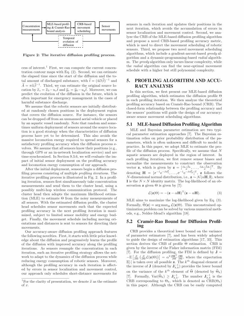
Figure 2: The iterative diffusion profiling process.

cess of interest.1 First, we can compute the current concen-tration contour maps with Eq. (2). Second, we can estimatethe elapsed time since the start of the diffusion and the to-

tal amount of discharged substance, with t = (4Dβ)−1 and

A = παβ−1. Third, we can estimate the original source lo-cation by xs = x0−ux t and ys = y0−uy t. Moreover, we canpredict the evolution of the diffusion in the future, which isoften important for emergency management in the cases ofharmful substance discharge.We assume that the robotic sensors are initially distribut-

ed at randomly chosen positions in the deployment regionthat covers the diffusion source. For instance, the sensorscan be dropped off from an unmanned aerial vehicle or placedby an aquatic vessel randomly. Note that random and some-times uniform deployment of sensors around the source loca-tion is a good strategy when the characteristics of diffusionprocess have yet to be determined. This also avoids themassive locomotion energy required to spread sensors for asatisfactory profiling accuracy when the diffusion process e-volves. We assume that all sensors know their positions (e.g.,through GPS or an in-network localization service) and aretime-synchronized. In Section 9.3.6, we will evaluate the im-pact of initial sensor deployment on the profiling accuracyand locomotion energy consumption of our approach.After the initial deployment, sensors begin a diffusion pro-

filing process consisting of multiple profiling iterations. Theiterative profiling process is illustrated in Fig. 2. In a profil-ing iteration, sensors first simultaneously take concentrationmeasurements and send them to the cluster head, using apossibly multi-hop wireless communication protocol. Thecluster head then adopts the maximum likelihood estima-tion (MLE) to estimate Θ from the noisy measurements ofall sensors. With the estimated diffusion profile, the clusterhead schedules sensor movements such that the expectedprofiling accuracy in the next profiling iteration is maxi-mized, subject to limited sensor mobility and energy bud-get. Finally, the movement schedule including moving ori-entations and distances is sent to sensors for directing theirmovements.Our accuracy-aware diffusion profiling approach features

the following novelties. First, it starts with little prior knowl-edge about the diffusion and progressively learns the profileof the diffusion with improved accuracy along the profilingiterations. As sensors resample the concentration in eachiteration, such an iterative profiling strategy allows the net-work to adapt to the dynamics of the diffusion process whilereducing energy consumption of robotic sensors. Moreover,although the profiling accuracy in each iteration is affect-ed by errors in sensor localization and movement control,our approach only schedules short-distance movements for

1For the clarity of presentation, we denote x as the estimateof x.

sensors in each iteration and updates their positions in thenext iteration, which avoids the accumulation of errors insensor localization and movement control. Second, we ana-lyze the CRB of the MLE-based diffusion profiling algorithmand propose a novel CRB-based profiling accuracy metric,which is used to direct the movement scheduling of roboticsensors. Third, we propose two novel movement schedulingalgorithms, which include a gradient-ascent-based greedy al-gorithm and a dynamic-programming-based radial algorith-m. The greedy algorithm only incurs linear complexity, whilethe radial algorithm can find the near-optimal movementschedule with a higher but still polynomial complexity.

5. PROFILING ALGORITHM AND ACCU-

RACY ANALYSISIn this section, we first present our MLE-based diffusion

profiling algorithm, which estimates the diffusion profile Θin each profiling iteration. We then analyze the theoreticalprofiling accuracy based on Cramer-Rao bound (CRB). Theclosed-form relationship between the profiling accuracy andthe sensors’ positions will guide the design of our accuracy-aware sensor movement scheduling algorithms.

5.1 MLE-based Diffusion Profiling AlgorithmMLE and Bayesian parameter estimation are two typi-

cal parameter estimation approaches [7]. The Bayesian es-timation relies on prior probability distribution of the pa-rameters, which is often unknown and difficult to model inpractice. In this paper, we adopt MLE to estimate the pro-file of the diffusion process. Specifically, we assume that Naquatic sensors are deployed in the region of interest. Ineach profiling iteration, we first remove sensor biases andnormalize the measurements to construct the observationvector z, which is given by z = [ z1−b1

σ, . . . , zN−bN

σ]T. By

denoting H = [σ−1e−βd21 , . . . , σ−1e−βd2N ]T, z follows the

N -dimensional normal distribution, i.e., z ∼ N (αH, I), whereI is the N ×N identity matrix. The log-likelihood of an ob-servation z given Θ is given by [7]:

L(z|Θ) = −(z− αH)T(z− αH). (3)

MLE aims to maximize the log-likelihood given by Eq. (3).

Formally, Θ(z) = argmaxΘ L(z|Θ). This unconstrained op-timization problem can be solved by various numerical meth-ods, e.g., Nelder-Mead’s algorithm [18].

5.2 Cramér-Rao Bound for Diffusion Profil-ing

CRB provides a theoretical lower bound on the varianceof parameter estimators [7], and has been widely adoptedto guide the design of estimation algorithms [17, 33]. Thissection derives the CRB of profile Θ estimation. CRB isgiven by the inverse of the Fisher information matrix (FIM)[7]. For the diffusion profiling, the FIM is defined by J =

−E[

∂∂Θ

(∂∂Θ

L(z|Θ))]

= α2 ∂HT

∂Θ∂H∂Θ

, where the expectation

E[·] is taken over all possible z. The kth diagonal element ofthe inverse of J (denoted by J−1

k,k) provides the lower bound

on the variance of the kth element of Θ (denoted by Θk)

[7]. Formally, Var(Θk) ≥ J−1k,k. The number J−1

k,k is the

CRB corresponding to Θk, which is denoted as CRB(Θk)in this paper. Although the CRB can be easily computed

via numerical methods, in order to guide the movements ofsensors, we will derive the closed-form CRB.Even though J is just a 4×4 matrix, deriving J−1 is chal-

lenging, because the N -dimensional joint distribution func-tion in Eq. (3) leads to high inter-node dependence. To sim-plify the discussion, we set up a Cartesian coordinate systemwith the origin at the source location and let (xi, yi) denotethe coordinates of sensor i. Note that the coordinates of thediffusion source and sensor i in the global coordinate systemare (x0, y0) and (x0 + xi, y0 + yi), respectively. We applymatrix calculus to derive the closed-form J and then deriveJ−1 by block matrix manipulations. Due to space limita-tion, the details of the derivations are omitted here and canbe found in [30]. To facilitate the representation of CRB,we first define several notations, i.e., xi, yi, LX1

, LX2, LY1

,and LY2

. First, xi is given by

xi =

N∑j=1

xj(d2j − d2i )e

−2βd2j

√N∑

m=1

N∑n=1

(d2m − d2n)2e−2β(d2m+d2n)

. (4)

By replacing xj in Eq. (4) with yj , we can define yi in asimilar manner. Moreover, LX1

, LY1are 1×N vectors, and

LX2, LY2

are N × 1 vectors. The ith elements of them are

LX1(i) = σ−1e−βd2i (xi + xi), LY1

(i) = σ−1e−βd2i (yi + yi),

LX2(i) = σ−1e−βd2i (xi − xi), LY2

(i) = σ−1e−βd2i (yi − yi).

Based on the above notation, the CRBs for the estimates ofx0 and y0 are given by

CRB(x0) = J−11,1 =

(4α2β2)−1

LX1LX2

−(LX1

LY2+LX2

LY1)2

4LY1LY2

, (5)

CRB(y0) = J−12,2 =

(4α2β2)−1

LY1LY2

−(LX1

LY2+LX2

LY1)2

4LX1LX2

. (6)

5.3 Profiling Accuracy MetricIn this section, we propose a novel diffusion profiling accu-

racy metric based on the CRBs derived in Section 5.2, whichwill be used to guide the movements of sensors in Section 6.Several previous works [23] adopt the determinant of theFIM as the accuracy metric, which jointly considers all theparameters. Such a metric requires the parameters to beproperly normalized to avoid biases. However, normalizingthe parameters with different physical meanings is highlyproblem-dependent. Moreover, as the closed-form determi-nant of the FIM is extremely complicated, the resulted sen-sor movement scheduling has to rely on the numerical meth-ods with high computational complexities [23], which is notsuitable for robotic sensors with limited resources. In thispaper, we propose a new profiling accuracy metric, denotedby ω, which is defined according to the sum of reciprocals ofCRB(x0) and CRB(y0). Formally,

ω =

1CRB(x0)

+ 1CRB(y0)

4α2β2= (1−ǫ) (LX1

LX2+ LY1

LY2) , (7)

where ǫ =(LX1

LY2+LX2

LY1)2

4LX1LX2

LY1LY2

. By adopting reciprocals, the

accuracy analysis can be greatly simplified. Note that as αand β are unknown but fixed in a particular profiling itera-tion, 4α2β2 in the denominator of Eq. (7) is a scaling factor.

Therefore, optimizing 1CRB(x0)

+ 1CRB(y0)

is equivalent to op-

timizing ω. As discussed in Section 5.1, we adopt the MLEto estimate Θ. The variance of the MLE result converges toCRB and hence a larger ω indicates more accurate estima-tion of x0 and y0. With the metric ω, the movements of sen-sors will be directed according to the accuracy of localizingthe diffusion source. In the rest of this paper, the term pro-filing accuracy refers to the metric ω defined in Eq. (7). Notethat our approach can also be applied to focus on the profil-ing accuracy of the elapsed time t and discharged substanceamount A, by applying the same matrix manipulations toobtain CRB(α) and CRB(β).

According to the derivations in Section 5.2, LX1, LY1

, LX2

and LY2depend on x0, y0, xi and yi. Therefore, ω is a func-

tion of the positions of the sensors and the diffusion source.As the location of the diffusion source, i.e., (x0, y0), is un-known to the network, it is impossible to compute the trueprofiling accuracy. In our approach, we compute ω based onthe estimated location of the diffusion source, i.e., (x0, y0),given by the MLE. As sensors are repositioned in each pro-filing iteration, the discrepancy between the true and esti-mated profiles is expected to be reduced along with the iter-ations. The profiling accuracy ω in Eq. (7) is still too com-plex for us to find efficient movement scheduling algorithms.Hence, we derive the approximation to Eq. (7). If sensors arerandomly distributed around the diffusion source, ǫ is closeto zero. By assuming a random sensor distribution and set-ting ǫ = 0, the profiling accuracy can be approximated as:

ω ≈N∑

i=1

ωi, ωi = σ−2e−2βd2i

(d2i − min

j∈[1,N ],j 6=id2j

), (8)

where ωi can be regarded as the contribution of sensor ito the overall profiling accuracy. As ωi depends on di andthe minimum distance to the source from other sensors, E-q. (8) highly reduces the inter-node dependence comparedwith Eq. (7). The accuracy of this approximation is validat-ed by extensive numerical results, which are omitted hereand available in [30]. In Section 9.3.5, we will evaluate theimpact of sensor deployment on the profiling accuracy whenthe sensor deployment deviates from random distributionaround the diffusion source.

6. DIFFUSION PROCESS PROFILING US-

ING ROBOTIC SENSORSIn this section, we formally formulate the movement schedul-

ing problem. Because of the limited mobility and ener-gy budget of aquatic mobile sensors, the sensor movementsmust be efficiently scheduled in order to achieve the maxi-mum profiling accuracy. As the power consumption of sens-ing, computation and radio transmission is significantly lessthan that of locomotion [26], in this paper we only considerthe locomotion energy. Moreover, as the locomotion energyis approximately proportional to the moving distance [3], wewill use moving distance to quantify the locomotion energyconsumption. To simplify the motion control of sensors, weassume that a sensor moves straight in each profiling itera-tion and the moving distance is always multiple of l meters,where l is referred to as step. We note that this model is mo-tivated by the locomotion and computation limitation typ-ically seen for aquatic sensor platforms. First, the locomo-tion of robotic fish is typically driven by closed-loop motioncontrol algorithms, resulting in constant course-correction

during movement. Second, each profiling iteration has shorttime duration. As a result, the assumption of sensor’s s-traight movement in an iteration does not introduce signifi-cant errors in the movement scheduling. As the estimationand movement are performed in an iterative manner, wewill focus on the movement scheduling in one profiling it-eration. Denote mi ∈ Z

+ and φi ∈ [0, 2π) as the numberof steps and movement orientation of sensor i in a profilingiteration, respectively. Our objective is to maximize the ex-pected profiling accuracy after sensor movements, subject tothe constraints on total energy budget and sensor’s individ-ual energy budget. The movement scheduling problem fordiffusion profiling is formally formulated as follows:

Movement Scheduling Problem. Suppose that a total ofM steps can be allocated to sensors and sensor i can moveat most Li meters in a profiling iteration. Find the alloca-tion of steps and movement orientations for all N sensors,i.e., mi, φi|i ∈ [1, N ], such that the profiling accuracy ω(defined by Eq. (7)) after sensor movements is maximized,subject to:

N∑

i=1

mi ≤ M, (9)

mi · l ≤ Li, ∀i. (10)

Eq. (9) upper-bounds the total locomotion energy in a pro-filing iteration. Eq. (10) can be used to constrain the en-ergy consumption of individual sensors. For instance, Li

can be specified according to the sensor’s residual energy.Moreover, Li can also be specified to ensure the delay of aprofiling iteration. If sensors move at a constant speed ofvm/s and a profiling iteration is required to be completedwithin τ seconds to achieve the desired temporal resolutionof profiling, Li can be set to Li = v · τ . As discussed in Sec-tion 4, the cluster head adopts MLE to estimate Θ, and thenschedules the movements of sensors such that the expectedω in the next profiling iteration is maximized, subject tothe constraints in Eqs. (9) and (10). An exhaustive searchto the above problem would yield an exponential complexitywith respect to N , which is O(( 2π

φ0· Li

l)N ) where φ0 is the

granularity in searching for the movement orientation. Sucha complexity is prohibitively high as the problem needs tobe solved in each profiling iteration by the cluster head. Inthe next section, we will propose an efficient greedy algorith-m and a near-optimal radial algorithm that are feasible tomote-class robotic sensor platform.

7. SENSOR MOVEMENT SCHEDULING AL-

GORITHMSIn this section, we propose an efficient greedy movement

scheduling algorithm based on gradient ascent and a near-optimal radial algorithm based on dynamic programming tosolve the problem formulated in Section 6.

7.1 Greedy Movement SchedulingGradient ascent is a widely adopted approach to find a

local maximum of a utility function. In this paper, we pro-pose a greedy movement scheduling algorithm based on thegradient ascent approach. We first discuss how to determinethe movement orientations for the sensors. Since the profil-ing accuracy ω given by Eq. (7) is a function of all sensors’positions, we can compute the gradient of ω with respect to

the position of sensor i (denoted by ∇iω), which is formally

given by ∇iω =[

∂ω∂xi

, ∂ω∂yi

]T. When all sensors except sensor

i remain stationary, the metric ω will increase the fastestif sensor i moves in the orientation given by ∇iω. There-fore, in the greedy movement scheduling algorithm, we letφi = ∠(∇iω). Note that sensors will move simultaneouslywhen the movement schedule is executed. We now discusshow to allocate the movement steps. The magnitude of ∇iω,denoted by ‖∇iω‖, quantifies the steepness of the metric ωwhen sensor i moves in the orientation ∠(∇iω) while othersensors remain stationary. Therefore, in the greedy algo-rithm, we propose to proportionally allocate the movementsteps according to sensor’s gradient magnitude. Specifically,

mi is given by mi = min

⌊

‖∇iω‖∑Ni=1

‖∇iω‖·M

⌋

,⌊

Li

l

⌋

. Note

that the⌊Li

l

⌋in the min operator satisfies the constraint

Eq. (10). This greedy algorithm has linear complexity, i.e.,O(N), which is preferable for the cluster head with limitedcomputational resource.

7.2 Radial Movement SchedulingIn this section, we propose a new movement scheduling

algorithm based on the approximations discussed in Sec-tion 5.3. In this algorithm, each sensor moves toward oraway from the estimated source location along the straightline connecting the estimated source location and the sen-sor’s current position. Hence, it is referred to as the radialalgorithm. We first discuss how to determine sensors’ move-ment orientations and then present a dynamic-programming-based algorithm for allocating movement steps.

From Eq. (8), the contribution of sensor i, ωi, depend-s on the minimum distance between the cluster head andother sensors. Because of such inter-node dependence, it isdifficult to derive the optimal distance for each sensor thatmaximizes the overall profiling accuracy ω. It can be shownthat the problem involves non-linear and non-convex con-strained optimization. Several stochastic search algorithms,such as simulated annealing, can find near-optimal solution-s. However, these algorithms often have prohibitively highcomplexities. In our algorithm, we fix the sensor closest tothe estimated source location and only schedule the move-ments of other sensors in each profiling iteration. As thesensor closest to the source receives the highest SNR, mov-ing other sensors will likely yield more performance gain.Moreover, this sensor can serve as the cluster head that re-ceives measurements from other sensors and computes themovement schedule. It is hence desirable to keep it station-ary due to its higher energy consumption in computationand communication. We note that the sensor closest to thesource may be different in each iteration after sensor move-ments, resulting in rotation of cluster head among sensors.By fixing the sensor closest to the source, the distance dithat maximizes the expected ωi, denoted by d∗i , can be di-rectly calculated by

d∗i =

√1

2β+ min

j∈[1,N ]d2j , ∀i 6= argmin

j∈[1,N ]

dj . (11)

Note that as β is a time-dependent variable, d∗i also changeswith time and hence should be updated in each profilingiteration. Eq. (11) allows us to easily determine the move-ment orientation of sensor i. Specifically, if di > d∗i , sensor iwill move toward the estimated source location; Otherwise,

sensor i will move in the opposite direction. Formally, bydefining δ = sgn(d∗i − di), we can express the movementorientation of sensor i as φi = ∠([δ · xi, δ · yi]

T).We now discuss how to allocate the movement steps. In

the rest of this section, when we refer to sensor i, we assumesensor i is not the closest to the estimated source location.After sensor i moves mi steps in the orientation of φi, itscontribution to the overall profiling accuracy is given by

ωi(mi) =(di + δ ·mi · l)

2 −minj∈[1,N ] d2j

σ2 · e2β(di+δ·mi·l)2, (12)

where minj∈[1,N ] d2j in Eq. (12) is a constant for sensor i,

and β can be predicted based on its current estimate tocapture the temporal evolution of the diffusion, i.e., β =

(1/β + 4 ·D · τ)−1. Given the radial movement orientationsdescribed earlier, the formulated problem is equivalent tomaximizing

∑i ωi(mi) subject to the constraints Eqs. (9)

and (10), which can be solved by a dynamic programmingalgorithm as follows.We number the sensors by 1, 2, . . . , N − 1, excluding the

sensor closest to the estimated source location. Let Ω(i,m)be the maximum ω when the first i sensors are allocated withm steps. Therefore, the dynamic programming recursionthat computes Ω(i,m) can be expressed as:

Ω(i,m) = max0≤mi≤⌊Li/l⌋

Ω(i− 1,m−mi) + ωi(mi) .

The initial condition of the above recursion is Ω(0,m) = 0for m ∈ [0,M ]. According to the above equation, at theith iteration of the recursion, the optimal value of Ω(i,m)is computed as the maximum value of ⌊Li/l⌋ cases whichhave been computed in previous iterations of the recursion.Specifically, for the case where sensor i moves mi steps, themaximum profiling accuracy ω of the first i sensors allocatedwith m steps can be computed as Ω(i−1,m−mi)+ωi(mi),where Ω(i− 1,m−mi) is the maximum ω of the first i− 1sensors allocated with m−mi steps. The maximum overallprofiling accuracy is given by ω∗ = maxm∈[1,M ] Ω(N−1,m).We now describe how to construct the movement sched-

ule using the above dynamic programming recursion. Themovement schedule of sensor i is represented by a pair (i,mi).For each Ω(i,m), we define a movement schedule S(i,m)initialized to be an empty set. The set S(i,m) is filled incre-mentally in each iteration when Ω(i,m) is computed. Specif-ically, in the ith iteration of the recursion, if Ω(i − 1,m −mx) + ωi(mx) gives the maximum value among all cases,we add a movement schedule (i,mx) to S(i,m). Formally,S(i,m) = S(i− 1,m−mx) ∪ (i,mx), where

mx = argmax0≤mi≤⌊vτ/l⌋

Ω(i− 1,m−mi) + ωi(mi) .

The complexity of the dynamic programming is O(

(N − 1)M2)

,where N is the number of sensors and M is the number ofallocatable movement steps in a profiling iteration.

8. DISCUSSIONS

8.1 Impact of Localization and Control ErrorsThe diffusion profiling process discussed in this paper suf-

fers from localization and control errors introduced by GPSmodule and robotic fish movement. However, our iterativeprofiling algorithm can largely avoid the accumulation ofsuch errors. First, to achieve desired temporal resolution of

profiling, as discussed in Section 6, we upper bound sensors’moving distances in a profiling iteration. Therefore, the clus-ter head only schedules short-distance movements for sensorsin each iteration, hence avoiding the accumulated error inmovement control. Moreover, the profiling algorithm avoid-s the accumulation of localization errors by having sensorsupdate their positions in each profiling iteration. Therefore,the cluster head always leverages the latest sensors’ positionsthat are corrupted only by the errors of current localization.As a result, our profiling algorithm is robust to the localiza-tion and control errors. In Section 9.3, we will evaluate theimpact of such errors on profiling accuracy using real datatraces of GPS and robotic fish movement.

8.2 Scalability of the Radial AlgorithmThe complexity of the dynamic programming algorithm p-

resented in Section 7.2 is O((N − 1)M2

). When the number

of sensors increases, it is desirable to increase the numberof allocatable movement steps. As the maximum movingdistance of a sensor is limited by its energy budget, M isoften a linear function of N , i.e., M ∼ O(N). As a result,the complexity will be O(N3). Such a complexity may leadto long computation delay at the cluster head, which jeop-ardizes the timeliness of the periodical profiling process. Abasic idea to reduce the computation delay is to bound thenumber of sensors in each cluster. Although many clusteringalgorithms can achieve this objective [11], we adopt a sim-ple clustering method, in which each node randomly assignsitself a cluster ID ranging from 1 to p, where p is the totalnumber of clusters. When a diffusion process is profiled bymultiple clusters, the dynamic programming procedures areexecuted separately in different clusters. To account for theinterdependence among clusters, the overall estimated pro-file can be calculated as the average of results from all clus-ters. In Section 9.2, we will evaluate the trade-off betweenexecution time and profiling accuracy of this algorithm.

9. PERFORMANCE EVALUATION

9.1 Evaluation MethodologyWe evaluate our approach through a combination of real

testbed experiments and trace-driven simulations. First, weimplement the MLE, greedy and radial algorithms on TelosBmotes and evaluate their overhead. The results provide in-sights into the feasibility of adopting advanced estimationand movement scheduling algorithms on mote-class roboticsensor platforms. Second, we validate the diffusion processmodel in Eq. (2) with real lab experiments of Rhodamine-Bdiffusion. Third, we evaluate the proposed profiling algo-rithm in extensive simulations based on real data traces.We collect three sets of traces, including GPS localization,robotic fish movement control, and on-water Zigbee wirelesscommunication. We analyze the impact of several importan-t factors on the profiling accuracy, including the temporalsampling scheme, the source location bias, the sensor den-sity, and the network communication overhead. Our resultsshow that our approach can accurately profile dynamic dif-fusion process with low communication overhead.

9.2 Overhead on Sensor HardwareWe have implemented the MLE and the two movement

scheduling algorithms in TinyOS 2.1.1 on TelosB platform[15] equipped with an 8MHz processor. We ported the C

0

20

40

60

80

100

5 10 15 20

Exec

uti

on

tim

eon

Tel

osB

(s)

The number of sensors N

MLEgreedyradial

Figure 3: Execution time on Telos-B versus the number of sensors N .

0

20

40

60

80

100

1 2 315300

15600

15900

16200

16500

Rel

ativ

eex

ecuti

on

tim

e(%

)

Pro

fili

ng

accu

racy

ω

The number of clusters p

relative execution timeω(radial) of p clusters

Figure 4: Execution time and pro-filing accuracy versus the number ofclusters p.

0

0.2

0.4

0.6

0.8

1

5 15 25 35 45 55

Pac

ket

rece

pti

on

rati

o(P

RR

)

Distance between sensors (meter)

Figure 5: Packet reception ra-tio (PRR) (90% confidence) versusdistance.

implementation of the Nelder-Mead algorithm [18] in GNUScientific Library (GSL) [2] to TinyOS to solve the opti-mization problem in MLE (see Section 5.1). The porting isnon-trivial because dynamic memory allocation and functionpointer are extensively used in GSL while these features arenot available in TinyOS. Our implementation of MLE re-quires 19KB ROM and 1KB RAM. When 10 sensors areto be scheduled, the two movement scheduling algorithmsrequire 1 and 8.8KB RAM, respectively. Fig. 3 plots theaverage execution time of the MLE, greedy and radial al-gorithms versus the number of sensors. We note that thecomplexity of MLE is O(N). For both movement schedul-ing algorithms, the execution time linearly increases withN , which is consistent with our complexity analysis. Theradial algorithm takes about 100 seconds to compute themovement schedule in a profiling iteration when N = 20.This overhead is reasonable compared with the movemen-t delay of low-speed mobile sensors. The greedy algorithmis significantly faster, and hence provides an efficient solu-tion when the timeliness is more important than profilingaccuracy. For the radial algorithm, 30% execution time isspent on computing a look-up table consisting of each sensori’s contribution, i.e., ωi(mi) in Eq. (12), given all possiblevalues of mi. There are several ways to further reduce thecomputational overhead. First, our current implementationemploys extensive floating-point computation. Our previousexperience shows that fixed-point arithmetic is significantlymore efficient on TelosB motes. Moreover, we can also adoptmore powerful sensor platforms as cluster head in the net-work. For instance, the projected execution time on Imote2[15] equipped with a 416MHz processor is within 2 secondsfor computing the movement schedule for 20 sensors.Fig. 4 plots the execution time and the profiling accuracy

of the scalable variant of radial approach, which is discussedin Section 8.2, versus the number of clusters, respectively.The left Y-axis is the ratio of execution time for p clusterswith respect to the case of a single cluster. We can see thatboth the execution time and profiling accuracy decrease withthe number of clusters. As discussed in Section 8.2, this isdue to the fact that simply averaging results from all clustersdoes not fully account for the inter-cluster dependence inthe accuracy of dynamic programming. Nevertheless, theradial algorithm of 2 and 3 clusters still outperforms thegreedy algorithm of a single cluster in terms of the profilingaccuracy.

9.3 Trace-Driven Simulations

9.3.1 Model Validation and Trace Collection

We collected four sets of data traces, which include chemi-cal diffusion, GPS localization errors, robotic fish movementcontrol, and on-water Zigbee wireless communication. First,we use the chemical diffusion traces to validate the diffusionprocess model in Eq. (2). To collect the traces, we dischargeRhodamine-B solution in saline water, and periodically cap-ture diffusion process using a digital camera. We assumethat the grayscale of a pixel in the captured image linearlyincreases with the concentration at the corresponding phys-ical location [27]. Therefore, the evolution of diffusion pro-cess can be characterized by the expansion of a contour giv-en a certain threshold of grayscale in the captured images.With the contour areas along the recorded shooting times,we can estimate D by linear regression. The detailed deriva-tions are available in [30]. Fig. 6 plots the captured imageswith contours marked in white. Fig. 7 plots the contour ar-eas observed in images and predicted by Eq. (2) versus t.We can see that the model in Eq. (2) well characterizes thediffusion of Rhodamine-B.

To evaluate the proposed profiling algorithms, we also col-lect traces of GPS localization errors, robotic fish movementcontrol and on-water Zigbee wireless communication. First,the data traces of GPS error are collected using two LinxGPS modules [12] in outdoor open space. We extract theGPS error by comparing the distance measured by GPSmodules with the groundtruth distance. The average GPSerror is 2.29meters. Second, the data traces of movementcontrol are collected with a robotic fish developed in our lab[26] (see Fig. 1). The movement of robotic fish is driven bya servo motor that is controlled by continuous pulse-widthmodulation waves. By setting the fish tail beating ampli-tude and frequency to 23 and 0.9Hz, the movement speedis 2.5m/min. We then have the fish swim along a fixed direc-tion in an experimental water tank, and derive the real speedby dividing the moving distance by elapsed time. Third, thedata traces of Zigbee communication are collected with twoIRIS motes2 by measuring the packet reception rate (PRR)on the wavy water surface of Lake Lansing on a windy day.We note that the PRR in such wavy water environment ismore dynamic than that in calm water environment, due

2The next generation of our robotic fish platform adopts thesame RF230 radio chip equipped on IRIS.

(a) Elapsed time t=3.5 s (b) Elapsed time t=18.1 s

Figure 6: Observations of the diffusion process ofRhodamine-B solution in saline water.

0.5

1.5

2.5

3.5

2 4 6 8 10 12 14 16 18 20

Conto

ur

area

(cm

2)

Elapsed time t (second)

observed in imagespredicted by Eq. (2)

Figure 7: Observed and predicted contour area of d-iffusing Rhodamine-B in saline water versus elapsedtime t.

to multipathing [5]. Specifically, we place the two motesabout 12 centimeters above the water surface, and measurethe PRR versus the distance between sensors. The result-s are plotted in Fig. 5. We note that the two IRIS motesachieve an average PRR of 0.8, when they are 37meters a-part. According to our experience, the communication rangeof IRIS on water surface decreases by about 50% comparedto that on land.

9.3.2 Simulation Settings

We conduct extensive simulations based on collected da-ta traces to evaluate the effectiveness of our approach. Thesimulation programs are written in Matlab. As discussedin Section 3.2, the effect of constant-speed advection is can-celed because the sensors and source location are in the sameinertial system. Therefore, we only simulate the diffusionprocess without advection. The diffusion source is at the o-rigin of the coordinate system, i.e., x0 = y0 = 0. The sensorsare randomly deployed in the square region of 200× 200m2

centered at the origin. The reading of a sensor is set tobe the sum of the concentration calculated from Eq. (2),the bias bi, and a random number sampled from the normaldistribution N (0, ς2). As discussed in Section 3.2, in eachprofiling iteration, a sensor samples K readings and outputsthe average of them as the measurement. The amount ofdischarged substance is set to be A = 0.7 × 106 cm3 (i.e.,0.7m3) unless otherwise specified. The diffusion coefficientis set to be D = 5,000 cm2/s. Note that the settings of Aand D are comparable to the real field experiments report-ed in [8] where 2 to 5m3 of diesel oil were discharged intothe sea and the estimated diffusion coefficient ranged from2,000 cm2/s to 7,000 cm2/s. The noise standard deviation isset to be ς = 1 cm3/m2, i.e., 1 cm3 discharged substance per

-100

-50

0

50

100

-100 -50 0 50 100

x (meter)

y(m

ete

r)

12

34

56

78

9

10

1112

13

14

15

1617

18

19 20diffusion source

sensors

(a) greedy: final ω = 15400

-100

-50

0

50

100

-100 -50 0 50 100

x (meter)

y(m

ete

r)

12

34

56

78

9

10

1112

13

14

15

1617

18

19 20diffusion source

sensors

(b) radial: final ω = 16400

Figure 8: Movement trajectories of 20 sensors in thefirst 15 profiling iterations.

unit area.3 To easily compare various movement schedulingalgorithms, we let the first profiling iteration always startat t = 1800 s, i.e., half an hour after the discharge. Att = 1800 s, the average received SNR is around 10/1. Therationale of this setting is that moving sensors too early(i.e., at low SNRs) leads to little improvement on profilingaccuracy, resulting in waste of energy. In practice, variousapproaches can be applied to initiate the profiling process,e.g., by comparing the average measurement to a thresholdthat ensures good SNRs. Other settings include l = 0.5m,τ = 60 s, v = 2.5m/min and K = 2, unless otherwise speci-fied.

We compare our approach with two additional baselinealgorithms in the evaluation. The first baseline (referred toas SNR-based) schedules the movements based on the SNRsreceived by sensors. The SNR received by sensor i (denot-ed by SNRi) is defined as c(di, t)/σ, where di and t can be

computed from the estimated profile Θ. In the SNR-basedscheduling algorithm, the sensors always move toward theestimated source location to increase the received SNRs.The movement steps are proportionally allocated accord-ing to sensors’ SNRs. The rationale behind this heuristic isthat the accuracy of MLE increases with SNR. The secondbaseline (referred to as annealing) is based on the simulat-ed annealing algorithm. Specifically, for given movementorientations φi|∀i, it uses the brutal-force search to findthe optimal step allocation under the constraints in Eqs. (9)and (10). It then employs a simulated annealing algorithmto search for the optimal movement orientations. However,it has exponential complexity with respect to the number ofsensors.

9.3.3 Sensor Movement Trajectories

We first visually compare the sensor movement trajecto-ries computed by the greedy and radial movement schedulingalgorithms. A total of 20 sensors are deployed. Fig. 8 showsthe movement trajectories of sensors in the first 15 profil-ing iterations. For a particular sensor, the circle denotes itsinitial position, the segments represent its movement trajec-tory of 15 profiling iterations, and the arrow indicates its

3As we adopt a 2-dimensional model to characterize the dif-fusion process, the physical unit of concentration is cm3/m2.As observed in the field experiments [8], diesel oil can pen-etrate down to several meters from the water surface. As aresult, the equivalent ς that accounts for the depth dimen-sion ranges from 0.1 cm3/m3 to 1 cm3/m3. Our setting isconsistent with the noise standard derivation of the crudeoil sensor Cyclops-7 [28], which is 0.1 cm3/m3.

0

1500

3000

4500

6000

7500

1800 2100 2400 2700

Pro

fili

ng

accu

racy

ω

Elapsed time t (second)

radialtrace-driven radial

annealinggreedy

trace-driven greedySNR-based

stationary

Figure 9: Profiling accuracy ω ver-sus elapsed time t.

0.5

1

1.5

2

1800 1920 2040 2160 2280 2400 2520 2640

Aver

age

var

iance

ofx0

andy0

(m2

)

Elapsed time t (second)

A = 0.7 × 106 cm3

A = 1.4 × 106 cm3

trace-driven radialannealing

trace-driven greedySNR-based

Figure 10: Average Var(x0) andVar(y0) versus elapsed time t.

0

1

2

3

4

5

6

7

0 5 10 15 20

Aver

age

var

iance

ofx0

andy0

(m2

)

The number of samplings K

trace-driven radialtrace-driven greedy

SNR-based

Figure 11: Average Var(x0) andVar(y0) versus the number of sam-plings K.

movement orientation in the 15th iteration. The sensor withno segments remains stationary during all 15 profiling iter-ations. We can see that, with the greedy algorithm, severalsensors (e.g., sensor 15, 16, and 17) have bent trajectories.This is because the movement orientation of each sensor isto maximize the gradient ascent of ω, hence not necessarilyto be aligned along the iterations. In the radial algorithm,sensors’ trajectories are more straight. This is because themovement orientation is along the direction determined bythe current sensor position and the estimated source locationthat is close to the true source location. Moreover, we findthat the radial algorithm outperforms the greedy algorithmin terms of profiling accuracy after the first 15 iterations. Inthe greedy algorithm, the orientation assignment and move-ment step allocation are based on the gradient derived fromthe current positions of sensors. Besides, the greedy algo-rithm does not account for the interdependence of sensorsin providing the overall profiling accuracy. As a result, itssolution may not lead to the maximum ω after the sensormovements and the temporal evolution of diffusion.

9.3.4 Profiling Accuracy

In the second set of simulations, we evaluate the accuracyin estimating the diffusion profile Θ. Total 10 sensors aredeployed and our evaluation lasts for 15 profiling iterations.Fig. 9 plots the profiling accuracy ω (defined in Eq. (7))

based on the estimated diffusion profile Θ. The curve la-beled with “stationary” is the result if all sensors alwaysremain stationary. Nevertheless, we can see that the pro-filing accuracy improves over time because of the temporalevolution of the diffusion. In Fig. 9, the curves labeled witha prefix “trace-driven” are the simulation results based onthe data traces of localization errors and robotic fish move-ment. Specifically, the position reading of a robotic sensor iscorrupted by a localization error randomly selected from theGPS error traces. When a robotic sensor moves, its speedis set to be a real speed that is randomly selected from thedata traces. We can see that, for both greedy and radial, thecurves with and without simulated movement control andlocalization errors almost overlap with each other. As ouriterative approach has no accumulated error, small move-ment control and localization errors have little impact onour approach. The radial algorithm outperforms the greedyand SNR-based algorithms by 16% and 50% in terms of ωat the 15th profiling iteration, respectively. And the accura-cy performance of the radial algorithm is very close to the

annealing algorithm that can find the near-optimal solution.However, we note that in each iteration of the annealing al-gorithm, a new look-up table needs to be computed due tochanged movement orientations. Hence its execution timehighly depends on the number of iterations that can be verylarge. Therefore, the annealing algorithm is infeasible onmote-class platforms.

Fig. 10 plots the average of Var(x0) and Var(y0) in eachprofiling iteration under various settings of the dischargedsubstance amount A. In order to evaluate the variances ineach profiling iteration, the sensors perform many roundsof MLE, where each round yields a pair of (x0, y0). TheVar(x0) and Var(y0) are calculated from all rounds. FromFig. 10, we find that the variances may increase (for theSNR-based scheduling algorithm) or fluctuate (for other ap-proaches) after several iterations. This is because the vari-ances are time-dependent due to the involving of α and βin CRB(x0) and CRB(y0). Moreover, we can see that thevariances decrease with A. As sensors receive higher SNRsin the case of higher A, our result consists with the intuitionthat the estimation error decreases with SNR. Comparedwith the SNR-based algorithm, the radial algorithm reducesthe variance in estimating diffusion source location by 36%for A = 0.7 × 106 cm3. Compared with the greedy algorith-m, the reductions are 12% and 18% for A = 0.7 × 106 and1.4 × 106 cm3, respectively. We also evaluate the accuracyin estimating the substance amount A and elapsed time t.Both the greedy and radial algorithms can achieve a high ac-curacy. For instance, the relative error in estimating A forradial algorithm is within 1.4%. Due to space limitation, de-tailed evaluation results are omitted here and can be foundin [30].

9.3.5 Impact of Sampling, Source Bias and NetworkDensity

We characterize the profiling error after 15 iterations bythe average of Var(x0) and Var(y0). Except for the evalua-tions on network density, a total of 10 sensors are deployed.In the temporal sampling scheme presented in Section 3.2,a sensor yields the average of K continuous samples as themeasurement to reduce noise variance. Fig. 11 plots theprofiling error versus K. We can see that the profiling er-ror decreases with K. The relative reductions of profilingerror by the radial algorithm with respect to the greedy andSNR-based algorithms are about 18% and 30%, respectively,when K ranges from 2 to 20.

0

2

4

6

8

10

12

5 15 25 35 50Diffusion source bias δ (m)

Aver

age

var

iance

ofx0

andy0

(m2

)trace-driven radial

trace-driven greedySNR-based

Figure 12: Average Var(x0) andVar(y0) versus source location biasδ.

0.2

0.4

0.6

0.8

1

1.2

1.4

1.6

1.8

2

10 15 20 25 30

Aver

age

var

iance

ofx0

andy0

(m2

)

The number of sensors N

trace-driven radialtrace-driven greedy

SNR-based

Figure 13: Average Var(x0) andVar(y0) versus the number of sensorsN .

600

800

1000

1200

1 2 3 40

1600

3200

4800

6400

8000

Tota

ldis

tance

toupper

bound

(m)

Pro

fili

ng

accu

racy

ω

The number of deployed quadrants

distance to upper boundω of deploymentsupper bound of ω

Figure 14: Impact of initial de-ployment on the profiling accura-cy.

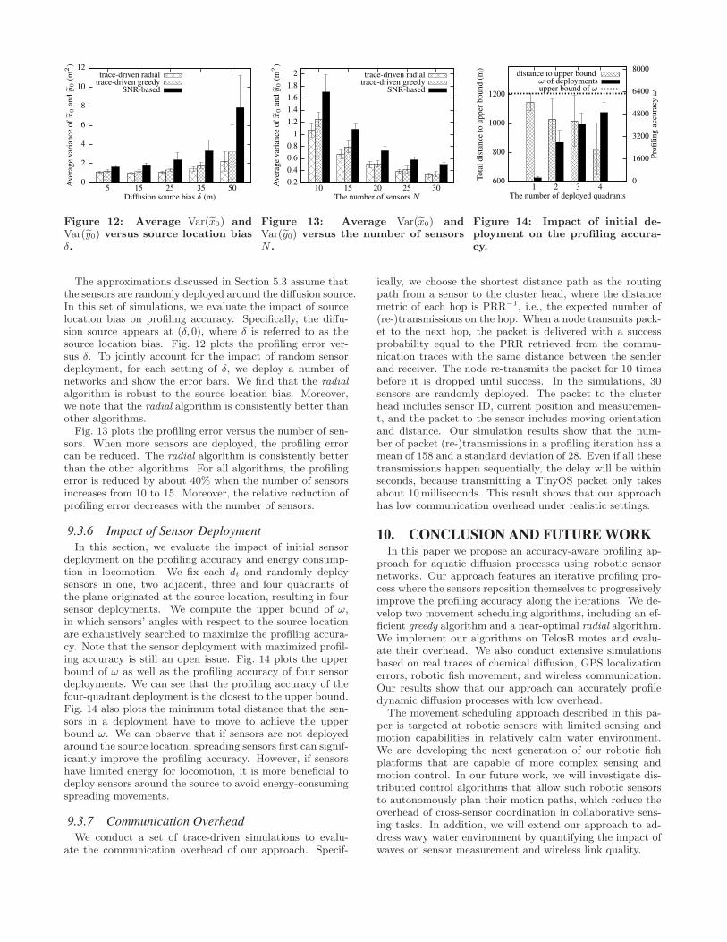
The approximations discussed in Section 5.3 assume thatthe sensors are randomly deployed around the diffusion source.In this set of simulations, we evaluate the impact of sourcelocation bias on profiling accuracy. Specifically, the diffu-sion source appears at (δ, 0), where δ is referred to as thesource location bias. Fig. 12 plots the profiling error ver-sus δ. To jointly account for the impact of random sensordeployment, for each setting of δ, we deploy a number ofnetworks and show the error bars. We find that the radialalgorithm is robust to the source location bias. Moreover,we note that the radial algorithm is consistently better thanother algorithms.Fig. 13 plots the profiling error versus the number of sen-

sors. When more sensors are deployed, the profiling errorcan be reduced. The radial algorithm is consistently betterthan the other algorithms. For all algorithms, the profilingerror is reduced by about 40% when the number of sensorsincreases from 10 to 15. Moreover, the relative reduction ofprofiling error decreases with the number of sensors.

9.3.6 Impact of Sensor Deployment

In this section, we evaluate the impact of initial sensordeployment on the profiling accuracy and energy consump-tion in locomotion. We fix each di and randomly deploysensors in one, two adjacent, three and four quadrants ofthe plane originated at the source location, resulting in foursensor deployments. We compute the upper bound of ω,in which sensors’ angles with respect to the source locationare exhaustively searched to maximize the profiling accura-cy. Note that the sensor deployment with maximized profil-ing accuracy is still an open issue. Fig. 14 plots the upperbound of ω as well as the profiling accuracy of four sensordeployments. We can see that the profiling accuracy of thefour-quadrant deployment is the closest to the upper bound.Fig. 14 also plots the minimum total distance that the sen-sors in a deployment have to move to achieve the upperbound ω. We can observe that if sensors are not deployedaround the source location, spreading sensors first can signif-icantly improve the profiling accuracy. However, if sensorshave limited energy for locomotion, it is more beneficial todeploy sensors around the source to avoid energy-consumingspreading movements.

9.3.7 Communication Overhead

We conduct a set of trace-driven simulations to evalu-ate the communication overhead of our approach. Specif-

ically, we choose the shortest distance path as the routingpath from a sensor to the cluster head, where the distancemetric of each hop is PRR−1, i.e., the expected number of(re-)transmissions on the hop. When a node transmits pack-et to the next hop, the packet is delivered with a successprobability equal to the PRR retrieved from the commu-nication traces with the same distance between the senderand receiver. The node re-transmits the packet for 10 timesbefore it is dropped until success. In the simulations, 30sensors are randomly deployed. The packet to the clusterhead includes sensor ID, current position and measuremen-t, and the packet to the sensor includes moving orientationand distance. Our simulation results show that the num-ber of packet (re-)transmissions in a profiling iteration has amean of 158 and a standard deviation of 28. Even if all thesetransmissions happen sequentially, the delay will be withinseconds, because transmitting a TinyOS packet only takesabout 10milliseconds. This result shows that our approachhas low communication overhead under realistic settings.

10. CONCLUSION AND FUTURE WORKIn this paper we propose an accuracy-aware profiling ap-

proach for aquatic diffusion processes using robotic sensornetworks. Our approach features an iterative profiling pro-cess where the sensors reposition themselves to progressivelyimprove the profiling accuracy along the iterations. We de-velop two movement scheduling algorithms, including an ef-ficient greedy algorithm and a near-optimal radial algorithm.We implement our algorithms on TelosB motes and evalu-ate their overhead. We also conduct extensive simulationsbased on real traces of chemical diffusion, GPS localizationerrors, robotic fish movement, and wireless communication.Our results show that our approach can accurately profiledynamic diffusion processes with low overhead.

The movement scheduling approach described in this pa-per is targeted at robotic sensors with limited sensing andmotion capabilities in relatively calm water environment.We are developing the next generation of our robotic fishplatforms that are capable of more complex sensing andmotion control. In our future work, we will investigate dis-tributed control algorithms that allow such robotic sensorsto autonomously plan their motion paths, which reduce theoverhead of cross-sensor coordination in collaborative sens-ing tasks. In addition, we will extend our approach to ad-dress wavy water environment by quantifying the impact ofwaves on sensor measurement and wireless link quality.

Acknowledgment

This research was supported in part by the U.S. NationalScience Foundation under grants ECCS-1029683 and CNS-0954039 (CAREER). We thank Ruogu Zhou for his contri-bution in traces collection and hardware design. We alsothank the anonymous reviewers providing the valuable feed-backs.

11. REFERENCES[1] http://www.infoplease.com/ipa/A0001451.html.

[2] GSL-GNU scientific library, 2011.

[3] D. Barrett, M. Triantafyllou, D. Yue,M. Grosenbaugh, and M. Wolfgang. Drag reduction infish-like locomotion. Journal of Fluid Mechanics,392(1):183–212, 1999.

[4] J. Chin, D. Yau, N. Rao, Y. Yang, C. Ma, andM. Shankar. Accurate localization of low-levelradioactive source under noise and measurementerrors. In The 6th ACM conference on EmbeddedNetworked Sensor Systems (SenSys), pages 183–196,2008.

[5] P. Corke, T. Wark, R. Jurdak, W. Hu, P. Valencia,and D. Moore. Environmental wireless sensornetworks. Proceedings of the IEEE, 98(11):1903–1917,2010.

[6] J. Crank. The mathematics of diffusion. OxfordUniversity Press, 1983.

[7] R. Duda, P. Hart, and D. Stork. PatternClassification. Wiley, 2001.

[8] A. Elliott. Shear diffusion and the spread of oil in thesurface layers of the north sea. Ocean Dynamics,39(3):113–137, 1986.

[9] C. Eriksen, T. Osse, R. Light, T. Wen, T. Lehman,P. Sabin, J. Ballard, and A. Chiodi. Seaglider: Along-range autonomous underwater vehicle foroceanographic research. IEEE Journal of OceanicEngineering, 26(4):424–436, 2001.

[10] Hydroid, LLC. REMUS: Autonomous technology foryour world.

[11] V. Kumar. Introduction to parallel computing.Addison-Wesley Longman Publishing Co., Inc., 2002.

[12] Linx Technologies. Linx GPS receiver module dataguide.

[13] N. March and M. Tosi. Introduction to Liquid StatePhysics. World Scientific Publishing, 2002.

[14] J. Matthes, L. Groll, and H. Keller. Sourcelocalization by spatially distributed electronic nosesfor advection and diffusion. IEEE Transactions onSignal Processing, 53(5):1711–1719, 2005.

[15] Memsic Corp. TelosB, IRIS, Imote2 datasheets.

[16] S. Murray. Turbulent diffusion of oil in the ocean.Limnology and oceanography, 17(5):651–660, 1972.

[17] A. Nehorai, B. Porat, and E. Paldi. Detection andlocalization of vapor-emitting sources. IEEETransactions on Signal Processing, 43(1):243–253,1995.

[18] J. Nelder and R. Mead. A simplex method for functionminimization. The Computer Journal, 7(4):308, 1965.

[19] L. Rossi, B. Krishnamachari, and C. Kuo. Distributedparameter estimation for monitoring diffusionphenomena using physical models. In The 1st annual

IEEE communications society conference on Sensor,Mesh and Ad Hoc Communications and Networks(SECON), pages 460–469, 2004.

[20] S. Ruberg, R. Muzzi, S. Brandt, J. Lane, T. Miller,J. Gray, S. Constant, and E. Downing. A wirelessinternet-based observatory: The real-time coastalobservation network (recon). In OCEANS, pages 1–6,2007.

[21] D. Rudnick, R. Davis, C. Eriksen, D. Fratantoni, andM. Perry. Underwater gliders for ocean research.Marine Technology Society Journal, 38(2):73–84, 2004.

[22] A. Singh, R. Nowak, and P. Ramanathan. Activelearning for adaptive mobile sensing networks. In The5th international conference on Information Processingin Sensor Networks (IPSN), pages 60–68, 2006.

[23] Z. Song, Y. Chen, J. Liang, and D. Ucinski. Optimalmobile sensor motion planning under nonholonomicconstraints for parameter estimation of distributedsystems. International Journal of Intelligent SystemsTechnologies and Applications, 3:277–295, 2007.

[24] S. Srinivasan, K. Ramamritham, and P. Kulkarni. Acein the hole: Adaptive contour estimation usingcollaborating mobile sensors. In The 7th internationalconference on Information Processing in SensorNetworks (IPSN), pages 147–158, 2008.

[25] R. Tan, G. Xing, J. Wang, and H. So. Exploitingreactive mobility for collaborative target detection inwireless sensor networks. IEEE Transactions onMobile Computing, 9(3):317–332, 2010.

[26] X. Tan. Autonomous robotic fish as mobile sensorplatforms: Challenges and potential solutions. MarineTechnology Society Journal, 45(4):31–40, 2011.

[27] E. Tsotsas and A. Mujumdar. Modern dryingtechnology, vol. 2, experimental techniques, 2009.

[28] Turner Designs Inc. Cyclops-7 user’s manual.

[29] S. Vijayakumaran, Y. Levinbook, and T. Wong.Maximum likelihood localization of a diffusive pointsource using binary observations. IEEE Transactionson Signal Processing, 55(2):665–676, 2007.

[30] Y. Wang, R. Tan, G. Xing, J. Wang, and X. Tan.Accuracy-aware aquatic diffusion process profilingusing robotic sensor networks. Technical report, CSEDepartment, Michigan State University, 2011.

[31] J. Weimer, B. Sinopoli, and B. Krogh. Multiple sourcedetection and localization in advection-diffusionprocesses using wireless sensor networks. In The 30thReal-Time Systems Symposium (RTSS), pages333–342, 2009.

[32] G. Xing, J. Wang, Z. Yuan, R. Tan, L. Sun,Q. Huang, X. Jia, and H. So. Mobile scheduling forspatiotemporal detection in wireless sensor networks.IEEE Transactions on Parallel and DistributedSystems, 21(12):1851–1866, 2010.

[33] T. Zhao and A. Nehorai. Distributed sequentialbayesian estimation of a diffusive source in wirelesssensor networks. IEEE Transactions on SignalProcessing, 55(4):1511–1524, 2007.