cloudsat precipitation proﬁling algorithm—model...

CloudSat Precipitation Profiling Algorithm—Model Description

CRISTIAN MITRESCU

Naval Research Laboratory, Monterey, California

TRISTAN L’ECUYER

Colorado State University, Fort Collins, Colorado

JOHN HAYNES

Monash University, Clayton, Australia

STEVEN MILLER

Cooperative Institute for Research in the Atmosphere, Fort Collins, Colorado

JOSEPH TURK

Jet Propulsion Laboratory, Pasadena, California

(Manuscript received 7 January 2009, in final form 17 December 2009)

ABSTRACT

Identifying and quantifying the intensity of light precipitation at global scales is still a difficult problem for

most of the remote sensing algorithms in use today. The variety of techniques and algorithms employed for

such a task yields a rather wide spectrum of possible values for a given precipitation event, further hampering

the understanding of cloud processes within the climate. The ability of CloudSat’s millimeter-wavelength

Cloud Profiling Radar (CPR) to profile not only cloud particles but also light precipitation brings some hope

to the above problems. Introduced as version zero, the present work uses basic concepts of detection and

retrieval of light precipitation using spaceborne radars. Based on physical principles of remote sensing, the

radar model relies on the description of clouds and rain particles in terms of a drop size distribution function.

Use of a numerical model temperature and humidity profile ensures the coexistence of mixed phases oth-

erwise undetected by the CPR. It also provides grounds for evaluating atmospheric attenuation, important at

this frequency. Related to the total attenuation, the surface response is used as an additional constraint in the

retrieval algorithm. Practical application of the profiling algorithm includes a 1-yr preliminary analysis of

global rainfall incidence and intensity. These results underscore once more the role of CloudSat rainfall

products for improving and enhancing current estimates of global light rainfall, mostly at higher latitudes,

with the goal of understanding its role in the global energy and water cycle.

1. Introduction

Clouds play an important role in the climate system

through complex, nonlinear feedback processes involving

radiation, chemistry, atmospheric dynamics and thermo-

dynamics, and surface–atmospheric coupling (Held and

Soden 2000). As an integral component of the earth’s

hydrological cycle, clouds are essential in sustaining many

forms of life on land through delivery of freshwater to the

surface and subsurface storage aquifers in the form of

precipitation. Given the widely varying spatial and tem-

poral distribution of precipitating cloud systems, satellite

remote sensing is the most practical option for monitor-

ing the global distribution and intensity of this quantity.

Moreover, given the three-dimensional structure of pre-

cipitation, active observing systems such as radars repre-

sent the best suited instruments for this purpose.

Corresponding author address: Cristian Mitrescu, Science Sys-

tems and Applications, Inc., One Enterprise Pkwy., Suite 200,

Hampton, VA 23666.

E-mail: [email protected]

MAY 2010 M I T R E S C U E T A L . 991

DOI: 10.1175/2009JAMC2181.1

� 2010 American Meteorological Society

The primary objective of CloudSat, a National Aero-

nautics and Space Administration (NASA) Earth System

Science Pathfinder satellite mission launched on 28 April

2006, is to provide, from space, the first global survey of

cloud vertical structure, layering, and content. Placed in

a sun-synchronous polar orbit (1330 local time ascending

node), CloudSat is capable of capturing the seasonal and

geographical distributions necessary to evaluate, un-

derstand, and ultimately improve the way clouds and

cloud feedbacks are handled within global weather and

climate forecast models (Stephens et al. 2002). With its

nominal 2-yr mission lifetime having been extended in for

an additional 3.5 yr (contingent on the health of the

spacecraft and sensor), the value of CloudSat measure-

ments to climate research continues to increase.

The ‘‘A-Train’’ constellation of satellites, of which

CloudSat is a member, is aimed at studying a full suite of

surface and atmospheric characteristics using an impres-

sive array of sensors, both active and passive that en-

compass a wide spectral range of frequencies. CloudSat

follows immediately behind the NASA Aqua satellite in

the A-Train. Aqua carries a suite of passive sensors such

as the Atmospheric Infrared Sounder/Advanced Micro-

wave Sounding Unit (AIRS/AMSU), Advanced Micro-

wave Scanning Radiometer for Earth Observing System

(AMSR-E), Clouds and the Earth’s Radiant Energy

System (CERES), and Moderate Resolution Imaging

Spectroradiometer (MODIS; http://aqua.nasa.gov). The

Cloud–Aerosol Lidar and Infrared Pathfinder Satellite

Observations (CALIPSO) satellite, carrying the Cloud-

Aerosol Lidar with Orthogonal Polarization (CALIOP)

lidar, trails closely behind CloudSat in tight formation

to achieve maximum overlap between the observations.

CALIOP is most sensitive to thin high-level cirrus,

aerosols, and boundary layer structures, providing a com-

plementary observation to CloudSat. Polarization and

Anisotropy of Reflectances for Atmospheric Sciences

coupled with Observations from a Lidar (PARASOL)

and Aura round off the A-Train formation.

This paper provides an update on progress to exploit

the sensitivity of CloudSat to light rainfall. Described

herein is an algorithm and methodology for quantifying

profiles of rain rate from measurements of radar back-

scatter. The technique is designed to augment the existing

suite of level-2 environmental data records produced by

CloudSat. In light of the multiple challenges (both algo-

rithmic and sensor hardware) associated with harnessing

the potential of this new sensor dataset, the results pre-

sented here are regarded as preliminary.

2. CloudSat’s 94-GHz observing system

CloudSat carries the Cloud Profiling Radar, a 94-GHz

nadir-pointing radar that has a sensitivity of around

228 dB, an 80-dB dynamic range, 240-m vertical reso-

lution (oversampled from a 480-m pulse length), and

a 1.7 km 3 1.3 km footprint. It samples 688 pulses to

form a single profile, with spacecraft motion over that

interval resulting in 1.1-km horizontal resolution. Unlike

ground-based radars that use centimeter wavelengths,

CloudSat’s millimeter operating wavelength (3 mm) pro-

vides sensitivity to lighter precipitation (missed by con-

ventional terrestrial weather radar systems) and even the

smaller ice and/or liquid particles composing the cloud

itself. From its satellite vantage point, the Cloud Profiling

Radar (CPR) beam is unobstructed by elevated terrain,

in contrast to ground-based radars. Although CloudSat

provides global coverage, its nadir-only viewing geometry

(nonscanning) results in ‘‘curtain’’ observations (2D slices

through the atmosphere) as opposed to the 3D volume

capability of a scanning sensor. Mitigating this limitation

are passive scanning sensors on the A-Train that offer a

wider 2D view of the scene within seconds–minutes of the

CPR observation. Moreover, the suite of all other geo-

stationary satellites offers the much needed spatial and

temporal continuum that complements the polar-orbiting

A-Train system. It follows that a combination of such

sensors can provide a nearly 3D scan of the atmosphere.

Combinations of these sensors are already being used to

characterize the global distribution of clouds (Mace et al.

2009) and to study the impact of aerosols on cloud optical

and microphysical properties (Lebsock et al. 2008). A

near-real-time application of CPR scans and associated

products are already being applied (Mitrescu et al. 2008).

3. CloudSat light precipitation profiling algorithm

The CPR on board CloudSat measures backscatter

reflectivity as a function of distance from both distributed

(i.e., hydrometeors) and solid (i.e., surface) targets. The

physical basis for the profiling algorithm resides in the

physical relationship between the return power, mea-

sured as a function of distance to the target, and the cloud,

precipitation, and surface properties. Given that its fre-

quency of operation (94 GHz) resides in a ‘‘dirty win-

dow’’ of the atmosphere where water vapor is slightly

absorptive, the measured signal is subject to both cloud

and atmospheric attenuation, which must be taken into

account. Because of the large volume sampled by the

CPR, the returned power at a given range often is in-

creased because of multiply-scattered photons. A com-

ponent of this multiply-scattered energy leads to a loss

of correct ranging capability, since the signal may have

come from other regions of the cloud. These effects in-

crease with the penetration depth and with the size of

cloud particles. As such, the ability to accurately sim-

ulate CPR observations (and thereby retrieve physical

992 J O U R N A L O F A P P L I E D M E T E O R O L O G Y A N D C L I M A T O L O G Y VOLUME 49

parameters) becomes increasingly more challenging for

range gates closer to the ground (i.e., farther away from

radar), which is where the precipitation occurs. The fol-

lowing subsections describe the procedures followed to

account for the various physical mechanisms influencing

the CPR measurements.

a. Cloud microphysical model

The purpose of developing a microphysical model is

to provide a physical description of the cloud vertical

structure allowing for model simulation of CPR mea-

surements and relating them to actual observations. For

the purposes of this retrieval, the focus is placed on those

key microphysical parameters to which the CPR holds

sensitivity. Since clouds are composed of a distribution of

particles (ice and/or water), of particular interest are

physical parameters such as number concentration, geo-

metrical dimension, mass, fall velocities, and rain rates.

However, given the limited information that the CPR

observing system offers, we are forced to focus our at-

tention to only one of the above parameters. All others

are to be parameterized in terms of this one particular

parameter. Since the present work focuses on retrieving

profiles of rain rates, this is the parameter of our choice.

Moreover, even if clouds at some point in their evolution

are in fact composed of a bimodal distribution of cloud

particles and precipitating particles, the radar is mostly

sensitive to the latter. Since a global parameterization

that uniquely describes this bimodal repartition is not yet

available, our choice is to represent clouds through a

single particle distribution, tuned to describing precipi-

tating particles. Obviously this approach would be valid

only in precipitating clouds.

Following L’Ecuyer and Stephens (2002), we assume

that all clouds can be described in terms of a Marshall–

Palmer droplet size distribution (DSD):

n(D)5 N0e�LD, (1)

where D is the diameter of the cloud particle. Using

mass–diameter and fall velocity–diameter power laws

(e.g., Liou 1992) that depend on a particle’s shape and

phase, one can relate the slope factor L to the rainfall

rate R:

L 5 aRb. (2)

Although not universal, and only for the purpose of

consistency with the work of Haynes et al. (2009), Table 1

shows the adopted values for these parameters. The

adopted units for R are millimeters per hour. In such

a way we can retrieve our unknown variable of interest,

the rainfall rate, from radar measurements (at each gate),

through an inversion algorithm that is described in sec-

tion 4. Since the rainfall rate is in fact related to the

characteristic diameter of (1), then the cloud mass can

also be evaluated. A quick sensitivity study of the above

equation with respect to the above parameters sheds

some light on the magnitude of error they may introduce.

As such, the rain-rate relative error is 1/b of the relative

errors in parameter a, and respectively jlnRj of the rela-

tive errors in parameter b. For the cases we encounter,

that translates into relative errors of R less than about

a factor of 7 of the relative errors of the above model

parameters. Given the wide statistical nature of all of the

above assumptions, the results that follow should only be

interpreted from this point of view and not particularized

for any given profile. This is still a work in progress that

needs improvement to properly describe clouds at all

scales of interest.

MIXED-PHASE PARAMETERIZATION

The microphysical model described above accounts

for both ice crystals and water drops. Whereas ice crys-

tals begin melting in regions where temperatures are

above freezing, physics allows for the liquid phase to

exist at temperatures as low as 2408C. As such, profiles

of temperature from numerical model runs are used to

determine the cloud phase. Therefore, we allow for the

possibility of mixed-phase clouds at temperature levels

between 2208 and 08C by imposing a precipitation mix-

ture of ice (98%) and water (2%) between these two

levels. To simulate the melting process, we gradually in-

crease the water percentage to 100% within three gates

following descent through the freezing level. For layers

with temperatures below 2208C, ice is the only phase

allowed in the current algorithm.

b. 94-GHz reflectivity model

Described here is the radiative model (i.e., radar

model) used to describe the scattering processes ob-

served by CloudSat. We represent the radar equation in

terms of modeled reflectivity Zm as follows:

Zm

5 Z 1 MS� PIA, (3)

where Z is the total backscatter reflectivity (from clouds,

or the surface), MS is the multiple-scattering contribu-

tion, and PIA is the path integrated attenuation that

accounts for the two-way energy loss due to extinction

TABLE 1. Rainfall retrieval microphysical parameters.

Parameter a (m) b N0 (m6)

Snow 4100 0.21 8.0 3 10218

Rain 1756 0.27 8.0 3 10218


(scattering plus absorption) processes occurring between

the radar and the range gate. Note that (3) is defined

at all levels (or range gates). Obviously, of particular

interest here are the range gates within the cloud and

precipitation. However, we are interested in the return

from the surface as well from the standpoint of its utility

in deriving PIA—a column-integrated parameter that

provides a natural constraint to the profiling algorithm

(L’Ecuyer and Stephens 2002). This will be developed

further below.

1) CLOUD PARTICLE RADAR MODEL

Under the assumption that the Mie regime is valid, the

cloud particle radiative properties at 94 GHz, defined by

(1) and (2), are computed as

X 5p

4

ð‘

0

n(D)QX

D2 dD, (4)

where X can be either the extinction, scattering, or

backscatter coefficients, while QX is the corresponding

Mie efficiency. The results are stored in the form of

discretized lookup tables (LUT) for both snow and rain,

as functions of temperature and rainfall rate. Future

versions of the algorithm will have to account for various

ice habits that can lead to significant departures from

Mie theory. Since the above calculations are based on

the distribution defined by (1), a sensitivity analysis

similar to that performed above yields a factor on the

order of 1/6b between relative errors in R and relative

errors in N0. We thus conclude that our retrieval model

is relatively constrained with respect to the knowledge

of forward model parameters.

2) PIA MODEL

PIA is significant at 94 GHz because of extinction

processes in the entire atmospheric column (clear or

cloudy):

PIA(H) 5 20 log(e)

ðH

0

sext

(z) dz, (5)

where sext is the sum of extinction coefficients of all

radiatively active atmospheric constituents and inte-

gration starts at the top of the atmosphere.

The principle gaseous atmospheric constituents that

must be accounted for are water vapor (H2O), O2, N2,

and their impacts to attenuation as a function of tem-

perature. Profiles of temperature and relative humidity

from a numerical weather model are coupled with

Liebe’s (1989) work to provide extinction information.

For cloudy atmospheres, the aforementioned LUT is

used to determine the appropriate extinction coefficient

given the rainfall rate and phase composition.

c. MS effects

Multiply scattered photons are present in most re-

motely sensed signals. Since these events do not scale

linearly with the scattering volume or its intrinsic single-

scattering properties, their contribution to the total sig-

nal can vary dramatically. Although numerous past

studies have grappled with this complicated problem

(e.g., Miller and Stephens 1999; Mitrescu 2005), evalu-

ations of MS contribution still lack in computational

efficiency and overall accuracy because of the highly

nonlinear nature of this problem. The MS problem is

further complicated by the antenna gain pattern and any

possible subgrid-scale inhomogeneity of the scattering

volume.

Given the top view that CPR has, the MS builds up

progressively as the signal penetrates deeper into the

cloud, starting with the second-order term. Although

higher-order terms may become dominant deeper into

the cloud, that happens only in the cases of deep con-

vective cloud systems, where we expect moderate–

heavy precipitation events. Since the goal of the present

work focuses on retrieving only light precipitation events

(i.e., precipitation rates below 5 mm h21), the multiple-

scattering effects can be neglected from the definition

of our forward model. However, as explained later on,

MS effects are flagged through the definition of the cost

function. Work is under way to implement a second-

order scattering model that accounts for antenna pattern

and is fast enough for semi-operational use.

d. Surface s0 model

Inspection of (3), applied at surface levels, suggests

the possibility of determining total column PIA from

measurements of surface return. Although complicated

by any MS effects, for a given surface type, the differ-

ence between surface measurements in a cloud-free at-

mosphere and a cloudy atmosphere is in fact total

column PIA:

PIAs

5 s0� s, (6)

where the subscript s indicates the methodology for

determining PIA. Here s0 is the surface return in clear

sky conditions corrected for atmospheric attenuation,

while s is the surface return for the particular cloudy

scene also corrected for atmospheric attenuation. The

basic assumption here is that the value for s0 can be

determined at all times, thus a universal constant for a

given surface type. Then one can use (6), seen as a quasi-

independent measurement, to constrain the computed

(5) as will be shown later.

Using surface response under clear sky conditions

(corrected for the atmospheric extinction), a s0 database


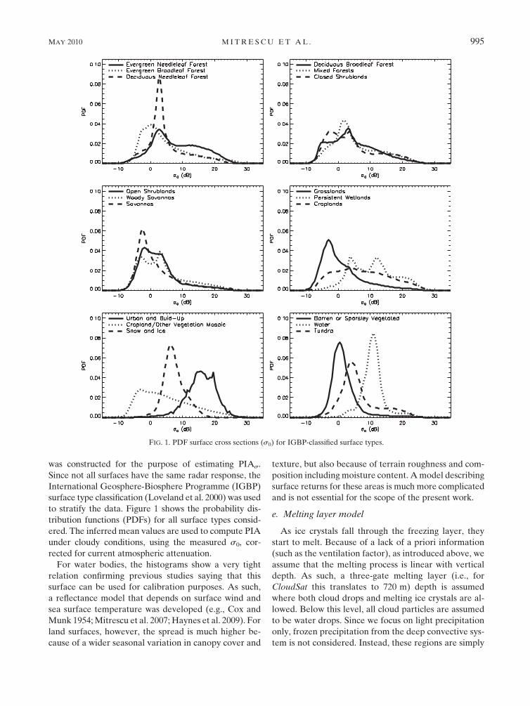
was constructed for the purpose of estimating PIAs.

Since not all surfaces have the same radar response, the

International Geosphere-Biosphere Programme (IGBP)

surface type classification (Loveland et al. 2000) was used

to stratify the data. Figure 1 shows the probability dis-

tribution functions (PDFs) for all surface types consid-

ered. The inferred mean values are used to compute PIA

under cloudy conditions, using the measured s0, cor-

rected for current atmospheric attenuation.

For water bodies, the histograms show a very tight

relation confirming previous studies saying that this

surface can be used for calibration purposes. As such,

a reflectance model that depends on surface wind and

sea surface temperature was developed (e.g., Cox and

Munk 1954; Mitrescu et al. 2007; Haynes et al. 2009). For

land surfaces, however, the spread is much higher be-

cause of a wider seasonal variation in canopy cover and

texture, but also because of terrain roughness and com-

position including moisture content. A model describing

surface returns for these areas is much more complicated

and is not essential for the scope of the present work.

e. Melting layer model

As ice crystals fall through the freezing layer, they

start to melt. Because of a lack of a priori information

(such as the ventilation factor), as introduced above, we

assume that the melting process is linear with vertical

depth. As such, a three-gate melting layer (i.e., for

CloudSat this translates to 720 m) depth is assumed

where both cloud drops and melting ice crystals are al-

lowed. Below this level, all cloud particles are assumed

to be water drops. Since we focus on light precipitation

only, frozen precipitation from the deep convective sys-

tem is not considered. Instead, these regions are simply

FIG. 1. PDF surface cross sections (s0) for IGBP-classified surface types.


flagged as heavy precipitation and skipped. An addi-

tional problem is encountered for cases of temperature

inversions. Here, we assume that the melting layer is the

topmost freezing layer. The scattering properties of melted

ice crystals are evaluated using the Maxwell–Garnett di-

electric mixing formula as introduced by Menenghini and

Liao (1996). We can thus write

�5 �i

1� 2 fA

11 fA, with A 5

�i� �

w

2�i1 �

w

, (7)

where f is the fractional melted volume while �i and

�w are the dielectric constants of ice and water, respec-

tively. Lookup tables as functions of rainfall rate and

melted fraction using (4) are generated. Although one

could argue that smaller crystals melt faster than larger

ones, the imposed melted fraction applies to the entire

distribution. By gradually increasing the water content

in this region, we in fact parameterize this process. As

such, both the melted and water DSDs are invariant

throughout the melting layer. Future versions of the

algorithm should seek better parameterization for de-

scribing this complex process. We also want to point out

that the above formulation is also being applied to the

ice–air mixture (using a mass–diameter relationship for

ice crystals).

4. The inverse model

The retrieval (or inversion) method chosen for in-

ferring profiles of precipitation rate is the optimal esti-

mation technique. Described in detail in many papers

(e.g., Jazwinsky 1970; L’Ecuyer and Stephens 2002;

Rodgers 1976), it uses the forward model to minimize

the cost function:

J 5 (R� Ra)TS�1

a (R� Ra) 1 (Z

o� Z

m)TS�1

Z (Zo� Z

m)

1 (PIA� PIAs)2S�1

s ,

(8)

where Zo is the observed radar reflectivity, Zm is the

modeled radar reflectivity, Sa is the a priori error co-

variance matrix with its diagonal terms set to 15 mm h21,

and SZ is the error covariance matrix associated with

observations that has its diagonal terms set to 2 dB2. We

note that the Sa formulation contains off-diagonal terms

that account for model error cross correlation between

various gates using an exponential decay function with

a correlation length set to 2.5 km. The quantity Ra is the

a priori estimate of the precipitation rate while R is the

rain-rate profile to be retrieved. As mentioned above,

additional information about modeled and observed PIA

due to hydrometeor attenuation is introduced via the last

term of the cost function using a fixed covariance Ss that

depends solely on the type of the surface (water or land).

If for water bodies PIAs can be determined with rela-

tively good accuracy (about 2 dB after wind and tem-

perature correction), for land surfaces it displays large

ambiguities (between 10 and 20 dB) that can create

convergence problems. It also shows that over land the

retrieval relies mostly on the measured profile. For this

reason adequate error covariance matrices must be used.

As such, one can control the information content to be

used for the retrieval problem, by filtering out the less

reliable information without completely ignoring it. As

this is still a work in progress, fine tuning is still be-

ing pursued. The above formulation seeks the solution

through successive iterations (i.e., a Gauss–Newton gra-

dient method) and does not require the introduction of

a separate inversion model since it only uses the forward

model formulation. A clear advantage of such an ap-

proach resides in its simplicity, flexibility, and universal-

ity. Moreover, additional constraints can be easily added

or removed from the above definition. The associated

covariance matrix of the retrieved profile is also provided:

SR

5 [S�1a 1 KTS�1

Z K 1 (PIA� PIAs)2S�1

s ]�1, (9)

where K is the kernel matrix or the weighting function

representing the sensitivity of the radar model to the

parameter being retrieved (R).

However, for complex problems, the optimal estima-

tion may become computationally demanding, particu-

larly for deep cloud structures, since it requires several

matrix computations. In addition, for these systems,

deep inside the cloud, the MS term becomes important.

When neglected, the retrieved scattering properties at

these gates are far larger than the expected values; this

effect increases further below because of a higher atten-

uation correction. As such, the iterative method quickly

becomes unstable as the cost function increases dramat-

ically. Therefore, the value of the cost function is used to

flag the MS effects, which are due to the presence of

heavy precipitation, as shown below.

5. Implementation

As explained above, CloudSat’s CPR is sensitive to

clouds and precipitation. Although not specifically sep-

arated in the proposed microphysical model, given the

strong dependence of the reflectivity field on the size of

the cloud particles, the precipitation regions yield higher

reflectivity values because of increased particle sizes.

Also, since the present algorithm seeks to evaluate cloud

precipitation that falls to the ground, a series of tests and


thresholds are being employed to discriminate between

precipitating and nonprecipitating clouds. The presence

of ground clutter creates a real problem, especially for

regions with low-level clouds over steep terrain. Tem-

perature data from numerical model runs (produced op-

erationally at the European Centre for Medium-Range

Weather Forecasts) are also used to flag the precipitation

phase. To keep consistency between the present profiling

algorithm and that developed by Haynes et al. (2009), we

adopt all the tests and thresholds defined within. More

details about these two precipitation techniques can be

downloaded from the Data Processing Center at Colo-

rado State University (http://CloudSat.cira.colostate.edu/

dataSpecs.php).

Given the size of the CloudSat files, and the proba-

bility of detecting any form of precipitation, one granule

is being processed somewhere between 10 and 30 min

on a 2.66-GHz dual-processor computer. Processing

time increases more than 100 times when MS effects are

considered, thus creating a serious limitation for near-

real-time processing. Work is under way for testing and

implementing fast multiple-scattering algorithms (e.g.,

Hogan 2008). Moreover, plans for adapting the attenu-

ation technique used for inferring rainfall rates as in-

troduced by Matrosov (2007) are being considered. That

would ensure a larger range of retrieved rainfall rates

using CloudSat’s 94-GHz CPR. In its present form,

however, we limit ourselves to retrieving only light pre-

cipitation with rainfall rates less than about 5 mm h21.

We also adopt the same rain likelihood flags as defined in

the constant column precipitation algorithm (2C-PC) of

Haynes et al. (2009). Despite this limitation, regions of

higher-intensity precipitation are still being identified in

the product but the algorithm does not provide quanti-

tative rain-rate estimates because of the MS problem

explained above.

6. Case study

This section summarizes results from the application

of the retrieval technique to actual CloudSat data. To

ensure quick validation to our results, we applied the

above retrieval algorithm to an orbital segment that was

collected when CloudSat was over the KLIX Next

Generation Weather Radar (NEXRAD), near New

Orleans, Louisiana, on 31 July 2006. Figure 2 (top panel)

shows the radar profile as recorded by the CPR. Evident

in the radar return is a nimbostratus cloud structure with

echo tops around 12 km and with its base obscured by

the rain signal. The bright band (BB), which can be clearly

distinguished, is just below the freezing level as in-

dicated by the temperature profile. Strong echoes near

the surface suggest that precipitation was likely. The

figure also suggests some entrainment near cloud top

and a change in the morphology of the cloud (i.e., a two-

layer cloud structure emerges) as the scan progresses

north. Figure 2 (second panel) demonstrates the profiling

capabilities of CloudSat and both the performances and

limitations of the present retrieval algorithm as it shows

profiles of the retrieved LWC and ice water content

(IWC) only for cases where the precipitation flag is set.

Because of the ground clutter problems, only gates above

1 km are being processed. The melting layer is again

clearly visible with retrieved values of up to 500 mg m23.

For demonstration purposes, Fig. 2 (third panel) shows

the unattenuated 94-GHz reflectivity field corresponding

to the above distribution of hydrometeors. This is nothing

more than the application of the forward model to the

retrieved LWC and IWC profiles. Moreover, the re-

flectivity field just below the bright band appears quasi-

uniform, a basic assumption employed by the other

two CloudSat precipitation models as mentioned be-

low. Moreover, the MS effects, neglected here, become

important for lower layers as the reflectivity field shows

values exceeding the 15-dBZ threshold. However, be-

cause of the additional constrain given by PIA, the re-

trieved rain rates are not far from those inferred using

other techniques and/or data. Figure 2 (bottom panel)

shows the rain rates inferred using CloudSat data applied

to three different algorithms and one using KLIX radar

data (extracted along CloudSat track). The latter is con-

verted into rainfall rates using the default (Z–R) relation-

ship for the Weather Surveillance Radar-1988 Doppler

(WSR-88D) radar network written as R 5 0.017Z0.714 and

shown with the green line. The black line denotes results

using the present algorithm. As an additional compari-

son, the blue line represents the approach described by

Matrosov (2007), where an extinction versus rain-rate

(k–R) relationship is being employed. However, since this

approach works only in regions below the bright band,

a gap in this data field is noted. The red line shows the rain

rates equivalent to a uniform cloud layer as described by

Haynes et al. (2009), where only PIA information is used

to infer a rain rate. Since this approach is only applicable

over ocean surfaces, the comparison can only be per-

formed for the first half of the data points (i.e., over

ocean). Finally, the along-CloudSat track rain rates as

retrieved using the AMSR-E passive microwave (PMW)

sensor onboard Aqua are presented with an orange line.

For this particular case, overall, the agreement between

all these various retrieval schemes (and/or sensors) is

satisfactory. However, we note pronounced spikes in the

retrieval around 1919:44 UTC. Here the BB signature is

obviously close to or below the measurement error and

the only option is the use of the NWP temperature

profile for its placement. Therefore, in the absence of


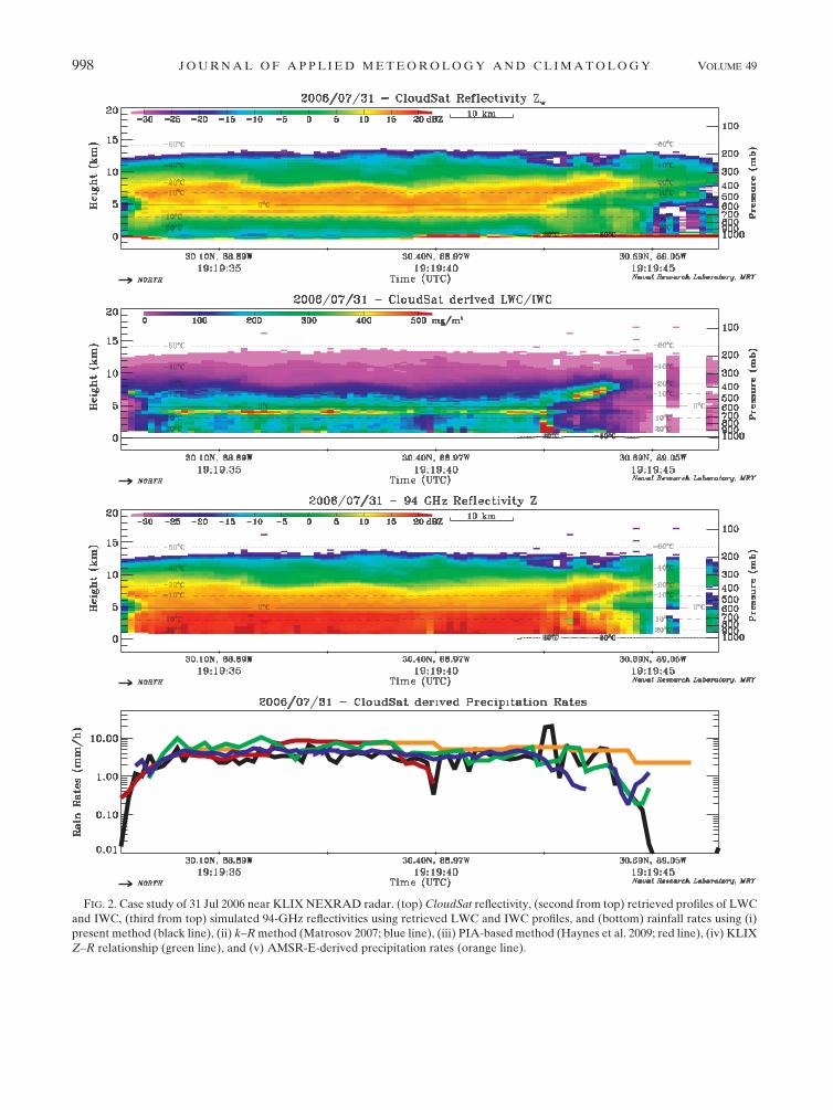
FIG. 2. Case study of 31 Jul 2006 near KLIX NEXRAD radar. (top) CloudSat reflectivity, (second from top) retrieved profiles of LWC

and IWC, (third from top) simulated 94-GHz reflectivities using retrieved LWC and IWC profiles, and (bottom) rainfall rates using (i)

present method (black line), (ii) k–R method (Matrosov 2007; blue line), (iii) PIA-based method (Haynes et al. 2009; red line), (iv) KLIX

Z–R relationship (green line), and (v) AMSR-E-derived precipitation rates (orange line).


a detectable BB, the forward model is thus slightly in-

correct in its BB formulation (i.e., placement and extent,

but also in describing the mixed phase). These artifacts

are amplified by the ground clutter effect and the neglect

of the MS term. Similar retrieval behavior, but less

pronounced, is seen in KLIX data. Also apparent is the

effect of the CPR footprint on the superior resolution of

the ground radars.

7. Statistical results

To further test the algorithm output, we run it for the

entire year of 2007. As explained above, since the MS

effects are neglected, the retrieval will not converge for

regions where rainfall rain rate is above or around

5 mm h21. These regions are flagged by the large values

in the cost function (8). Although no retrieved values are

reported in these cases, they are flagged as heavy pre-

cipitation regions. As such, we can distinguish three

regions of interest: clear, light precipitation, and heavy

precipitation. The retrieval runs on a global domain,

regardless of the underlying surface, or the presence of

a melting layer, or precipitation type that can somehow

be seen as a limiting factor. However, as mentioned

above, even if the aim of the paper is to introduce the

grounds for a precipitation profiling algorithm, given

the limitations of both the observing system as well as

the crudeness of the forward model, the results should

be interpreted with care.

As mentioned in the previous section, two other pre-

cipitation algorithm datasets are available: the 2C-PC

and the AMSR-E PMW precipitation product. Keeping

in mind that none of these three algorithms represents

the ground truth, the following discussion only contrasts

their output. Since precipitation is characterized by both

intensity and incidence, we decided to present this com-

parison study as divided into three main intensity-based

categories: (i) very light precipitation with rain rates less

than 1 mm h21; (ii) light–moderate precipitation with

rain rates between 1 and 5 mm h21; and (iii) heavy

precipitation with rain rates more than 5 mm h21. The

probability of rainfall in each of these categories as in-

ferred by all three algorithms is presented in Figs. 3, 4,

and 5, where each of the three panels (from top to bot-

tom) shows, in order, outputs from the present, 2C-PC,

and AMSR-E PMW algorithms, respectively. Despite

possible problems due to differences in ground resolution,

for consistency purposes, only AMSR-E pixels closest

to the CloudSat footprint were considered. Given the

sampling geometry that CPR has combined with the

A-Train orbital pass characteristics, the results capture

only a global 0130–1330 local time snapshot of the pre-

cipitation field. Overall, similar precipitation patterns and

regions can be observed in all three intensity-based cat-

egories, although the frequency of occurrence can vary

dramatically form one category to another and/or one

algorithm to another. Associated with either short-lived

convective regions or more persistent frontal regions,

light precipitating clouds are a common feature within

the general weather pattern features. Clearly discern-

ible are the Southern Hemisphere (SH) storm tracks—a

manifestation of the zonality in circulation—which pro-

duce considerable amounts of very light precipitation,

mostly due to frontal activity. Not as clearly defined are

the precipitating events associated with the Northern

Hemisphere (NH) storm tracks, influenced by the larger

distribution of land surfaces. As with the SH, a wave

structure due to frontal passages is visible. The inter-

tropical convergence zone (ITCZ) around the equator is

also well captured despite the decrease in spatial cov-

erage due to the polar orbit placement. Also captured

is the South Pacific convergence zone (SPCZ) as well as

the precipitation due to the monsoon cycle in the Arabian

Sea and Bay of Bengal. Over land, we note the both con-

vective and orographically induced precipitation features

over elevated regions in South America, Africa, and Tibet

due to the higher frequency and/or longer lifetime that

such cloud systems have. On the opposite side, low (or

nonexistent) precipitation regions like subtropical belts,

Australia, the Arabic Peninsula, or the Sahara are also

being resolved by this analysis. However, because of the

ground clutter problem, well known low marine stratus

regions, like those near California, Chile, West Africa,

etc., that have the potential of producing light precipi-

tation are misdiagnosed by the CPR. Since that happens

to all the low clouds over the entire globe, caution is re-

quired when interpreting these results.

Figure 3 shows the incidence of very light precipitation.

Somehow expected, the present algorithm (top panel)

contrasts the most with the other two methods. It clearly

identifies the SH and NH storm tracks as the most per-

sistent precipitation regions, with probability rates that

exceed 20%. In this case, we show all possible very light

precipitating events (i.e., retrieved reflectivities at the

lowest bin with values greater than 215 dBZ). Although

very light (with average rain rates less than 0.5 mm h21),

these regions may exert an important influence on the

global heating rates and the nonlinear cloud–climate in-

teractions. Very light precipitation events over ocean

bodies clearly exceed those over land surfaces. These

findings are in sharp contrast to the other two methods.

The 2C-PC method (middle panel), tuned only to liquid

precipitation, shows a decrease in precipitation events as

we move poleward, due to an increase in solid precip-

itation events. As expected, the AMSR-E PMW–based

algorithm (bottom panel) fails to reveal most of the very


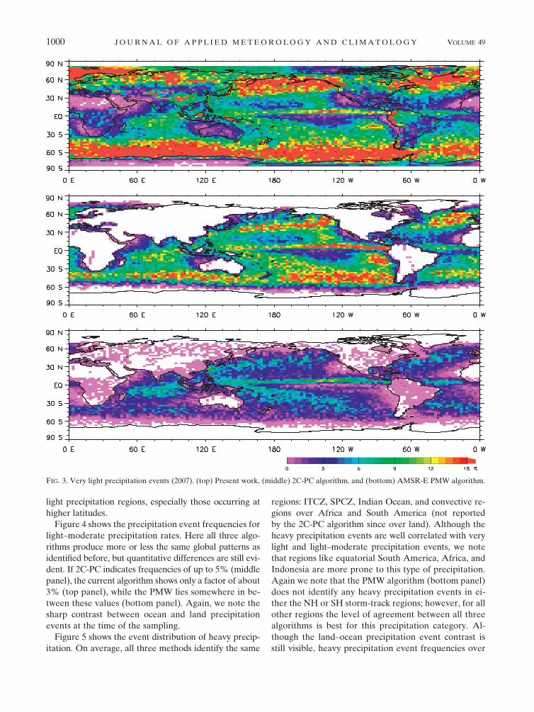
light precipitation regions, especially those occurring at

higher latitudes.

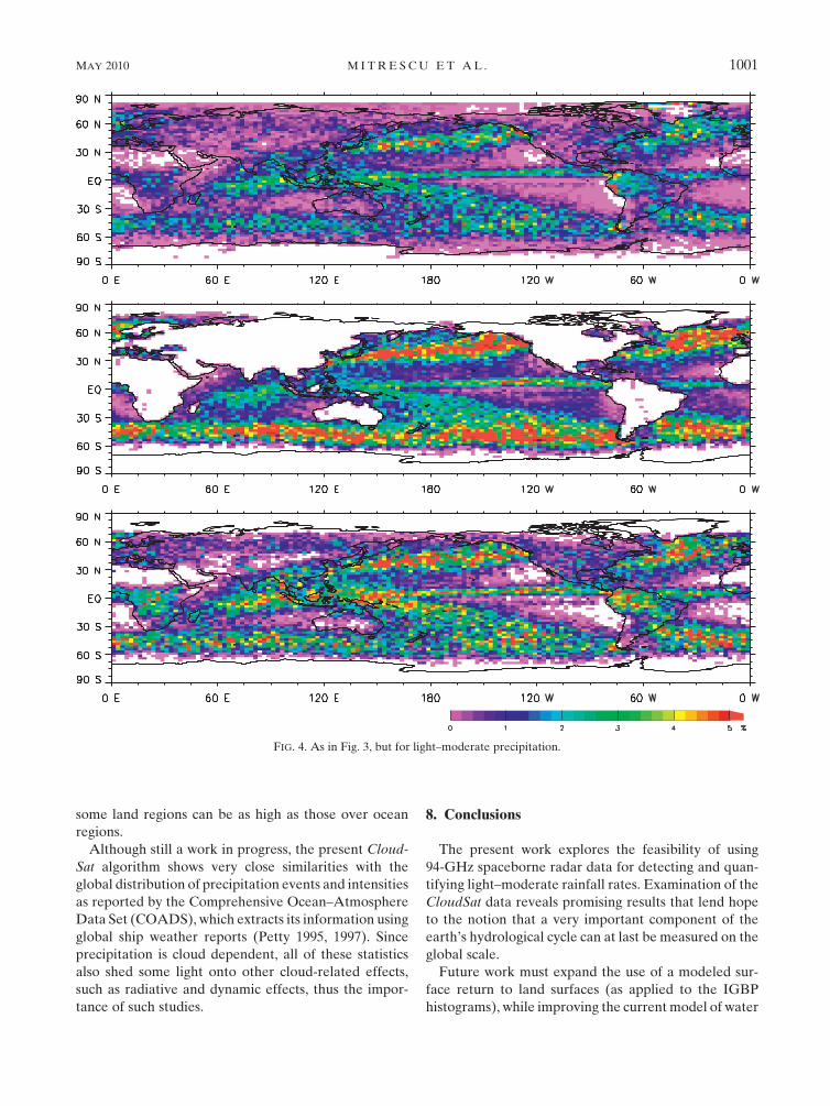
Figure 4 shows the precipitation event frequencies for

light–moderate precipitation rates. Here all three algo-

rithms produce more or less the same global patterns as

identified before, but quantitative differences are still evi-

dent. If 2C-PC indicates frequencies of up to 5% (middle

panel), the current algorithm shows only a factor of about

3% (top panel), while the PMW lies somewhere in be-

tween these values (bottom panel). Again, we note the

sharp contrast between ocean and land precipitation

events at the time of the sampling.

Figure 5 shows the event distribution of heavy precip-

itation. On average, all three methods identify the same

regions: ITCZ, SPCZ, Indian Ocean, and convective re-

gions over Africa and South America (not reported

by the 2C-PC algorithm since over land). Although the

heavy precipitation events are well correlated with very

light and light–moderate precipitation events, we note

that regions like equatorial South America, Africa, and

Indonesia are more prone to this type of precipitation.

Again we note that the PMW algorithm (bottom panel)

does not identify any heavy precipitation events in ei-

ther the NH or SH storm-track regions; however, for all

other regions the level of agreement between all three

algorithms is best for this precipitation category. Al-

though the land–ocean precipitation event contrast is

still visible, heavy precipitation event frequencies over

FIG. 3. Very light precipitation events (2007). (top) Present work, (middle) 2C-PC algorithm, and (bottom) AMSR-E PMW algorithm.


some land regions can be as high as those over ocean

regions.

Although still a work in progress, the present Cloud-

Sat algorithm shows very close similarities with the

global distribution of precipitation events and intensities

as reported by the Comprehensive Ocean–Atmosphere

Data Set (COADS), which extracts its information using

global ship weather reports (Petty 1995, 1997). Since

precipitation is cloud dependent, all of these statistics

also shed some light onto other cloud-related effects,

such as radiative and dynamic effects, thus the impor-

tance of such studies.

8. Conclusions

The present work explores the feasibility of using

94-GHz spaceborne radar data for detecting and quan-

tifying light–moderate rainfall rates. Examination of the

CloudSat data reveals promising results that lend hope

to the notion that a very important component of the

earth’s hydrological cycle can at last be measured on the

global scale.

Future work must expand the use of a modeled sur-

face return to land surfaces (as applied to the IGBP

histograms), while improving the current model of water

FIG. 4. As in Fig. 3, but for light–moderate precipitation.


surface reflectivity return. Also, resulting in part from

the large size of the sampled volume by the CPR sensor

compared to the ground radars, the effect of multiply-

scattered radiation must be taken into account (partic-

ularly in moderate rain regimes), either in terms of a

filter or an account made in the forward model based, for

example, on Monte Carlo simulations. The MS effect is

most pronounced at the farthest range gates where sur-

face rain rates are being evaluated, and increases dra-

matically with the amount of cloud–rainwater mass

residing in the column above. Moreover, an improved

algorithm for brightband detection and a more realistic

mixed-phase description are being tested for the next

versions of the CloudSat precipitation profiling algorithm.

Our ultimate goal is to produce a global quantitative

analysis of light precipitation for the entire CloudSat

mission. Since CloudSat is in a sun-synchronous or-

bit (1330 local time, ascending node), it should be ac-

knowledged that precipitation estimates are biased by

nonuniform diurnal sampling. Moreover, because of the

ground clutter that is present in the CloudSat signal we

are compelled at this early stage in data processing to

consider only radar returns from gates that are approx-

imately 1.25 km and higher above the surface for char-

acterizing surface rainfall. Thus, shallow, low-level

clouds (predominantly marine stratocumulus systems)

were excluded from these precipitation statistics. How-

ever, a new clutter filter approach should partially alleviate

FIG. 5. As in Fig. 3, but for heavy precipitation.


this problem and help push this limit somewhere close to

the 720-m range. Despite these shortcomings, these pre-

liminary findings are encouraging as they correlate well

with the other CloudSat precipitation algorithm (2C-PC),

AMSRE-E PMW algorithm, and/or ship observations

(COADS). These positive results not only add quantita-

tive information to the general knowledge of clouds and

precipitation, but also help to place CloudSat in the con-

text of better-known precipitation sensors.

Acknowledgments. The support of our sponsors,

NASA Earth Science Division Radiation Sciences Pro-

gram CloudSat light precipitation project (NNG07H43i),

and the Office of Naval Research under Program Ele-

ment PE-0602435N, is gratefully acknowledged.

REFERENCES

Cox, C., and W. Munk, 1954: Measurements of the roughness of the

sea surface from photographs of the sun’s glitter. J. Opt. Soc.

Amer., 144, 838–850.

Haynes, J. M., T. S. L’Ecuyer, G. L. Stephens, S. D. Miller,

C. Mitrescu, N. B. Wood, and S. Tanelli, 2009: Rainfall re-

trieval over the ocean with spaceborne W-band radar. J. Geo-

phys. Res., 114, D00A22, doi:10.1029/2008JD009973.

Held, I. M., and B. J. Soden, 2000: Water vapor feedback and global

warming. Annu. Rev. Energy Environ., 25, 441–475.

Hogan, R., 2008: Fast lidars and radar multiple-scattering models.

Part I: Small-angle scattering photon using the photon variance–

covariance method. J. Atmos. Sci., 65, 3621–3635.

Jazwinsky, A. H., 1970: Stochastic Processes and Filtering Theory.

Academic Press, 376 pp.

Lebsock, M. D., G. L. Stephens, and C. Kummerow, 2008: Multi-

sensor satellite observations of aerosol effects on warm clouds.

J. Geophys. Res., 113, D15205, doi:10.1029/2008JD009876.

L’Ecuyer, T., and G. L. Stephens, 2002: An estimation-based pre-

cipitation retrieval algorithm for attenuating radars. J. Appl.

Meteor., 41, 272–285.

Liebe, H., 1989: MPM89–An atmospheric mm-wave propagation

model. Int. J. Infrared Millimeter Waves, 10 (6), 631–650.

Liou, K. N., 1992: Radiation and Cloud Processes in the Atmo-

sphere. Oxford University Press, 487 pp.

Loveland, T. R., B. C. Reed, J. F. Brown, D. O. Ohlen, Z. Zhu,

L. Yang, and J. W. Merchant, 2000: Development of a global

land cover characteristics database and IGBP DISCover

from 1 km AVHRR data. Int. J. Remote Sens., 21 (6–7), 1303–

1330.

Mace, G. G., Q. Zhang, M. Vaughan, R. Marchand, G. Stephens,

C. Trepte, and D. Winker, 2009: A description of hydrometeor

layer occurrence statistics derived from the first year of

merged CloudSat and CALIPSO data. J. Geophys. Res., 114,

D00A26, doi:10.1029/2007JD009755.

Matrosov, S. Y., 2007: Potential for attenuation-based estimations

of rainfall rate from CloudSat. Geophys. Res. Lett., 34, L05817,

doi:10.1029/2006GL029161.

Menenghini, R., and L. Liao, 1996: Comparisons of cross sections

for melting hydrometeors as derived from dielectric mixing

formulas and a numerical method. J. Appl. Meteor., 35, 1658–

1670.

Miller, S. D., and G. L. Stephens, 1999: Multiple scattering effects

in the lidar pulse stretching problem. J. Geophys. Res., 104(D18), 22 205–22 220.

Mitrescu, C., 2005: Lidar model with parameterized multiple

scattering for retrieving cloud optical properties. J. Quant.

Spectrosc. Radiat. Transfer, 94, 210–224.

——, J. M. Haynes, T. L’Ecuyer, S. D. Miller, and J. Turk, 2007: Light

rain retrievals using CloudSat 94-GHz radar data–Preliminary

results. Preprints, 14th Symp. on Meteorological Observation and

Instrumentation and 16th Conf. on Applied Climatology, San

Antonio, TX, Amer. Meteor. Soc., JP2.6. [Available online at

http://ams.confex.com/ams/pdfpapers/117883.pdf.]

——, S. D. Miller, J. Hawkins, T. L’Ecuyer, J. Turk, P. Partain, and

G. L. Stephens, 2008: Near-real-time applications of CloudSat

data. J. Appl. Meteor. Climatol., 47, 1982–1994.

Petty, G. W., 1995: Frequencies and characteristics of global oce-

anic precipitation from shipboard present-weather reports.

Bull. Amer. Meteor. Soc., 76, 1593–1616.

——, 1997: An intercomparison of oceanic precipitation frequen-

cies from 10 special sensors microwave/imager rain rate al-

gorithms and shipboard present weather reports. J. Geophys.

Res., 102, 1757–1777.

Rodgers, C., 1976: Retrievals of atmospheric temperature and

composition from remote measurements of thermal radiation.

Rev. Geophys. Space Phys., 14, 609–624.

Stephens, G. L., and Coauthors, 2002: The CloudSat mission and

the A-Train: A new dimension of space-based observations of

clouds and precipitation. Bull. Amer. Meteor. Soc., 83, 1771–

1790.


cloudsat precipitation proﬁling algorithm—model...

Documents