accounting for flexibility in power system planning with
TRANSCRIPT

KULeuven Energy Institute
TME Branch
WP EN2013-08
Accounting for flexibility in power system planning with renewables
A. Belderbos, E. Delarue
TME WORKING PAPER - Energy and Environment Last update: August 2013
An electronic version of the paper may be downloaded from the TME website:
http://www.mech.kuleuven.be/tme/research/

1
Accounting for flexibility in power system planning with renewables
Andreas Belderbos, Erik Delarue*
University of Leuven (KU Leuven) Energy Institute, TME branch (Applied Mechanics and Energy Conversion), Celestijnenlaan 300A box 2421 / B-3001 Leuven / Belgium
E-mail addresses: [email protected] ; [email protected]
* Corresponding author:
Erik Delarue
University of Leuven (KU Leuven) Energy Institute, TME branch (Applied Mechanics and Energy Conversion), Celestijnenlaan 300A box 2421
B-3001 Leuven
Belgium
Tel.: +32 16 322511; fax: +32 16 322985.

2
Abstract
Due to the increasing deployment of intermittent renewables, the residual load profile, as seen by the dispatchable generation units, becomes lower and more volatile. This paper introduces a new system planning model with an individual power plant resolution, taking into account technical operational constraints. The objective of this model is to determine the optimal set of generation units, able to serve a given demand. An initial solution is obtained from a classical screening curve model, and from a model using mixed integer linear programming (MILP). These initial solutions are perturbed and combined with an operational model to further improve and validate the solution. The evolution of the optimal amount of generation capacity as a function of the installed wind capacity is examined in a case study. As the share of wind power increases in the portfolio, a shift takes place from base load generation towards mid and peak load. This shift is triggered both by the lower demand and the increasing volatility. Hence, this demonstrates that operational constraints of power plants (individual basis) have an important impact on the configuration of the optimal generator set, and need being considered.
Key-words: Power system planning; renewables; screening curve; unit commitment; wind power.

3
1 Introduction
Worldwide, electricity generation systems are undergoing major changes. The share of renewable energy sources (RES) is growing significantly, mainly driven by growing concerns on global warming and for reasons of strategic energy security. These RES, however, often have an intermittent profile. Their output is predictable only to a limited extent, and it is variable, not or only in a limited way dispatchable (e.g., wind turbines can be curtailed, reducing their output). The impact of these RES on the system is twofold: first, they reduce the residual load (i.e., the original load with RES generation subtracted). Second, also more flexibility is required to deal with the higher variability of the residual load. Hence, these effects need to be accounted for in both power system optimization [1-3].
Planning and operating of modern electric power systems comprehends several complex and interlinked tasks. These tasks can be divided in three main groups, depending on the considered time horizon. A first group includes long-term resource and equipment planning which targets time ranges from one year to several decades. Examples are investment planning, transmission and distribution planning and long range fuel planning. A second group contains short-term operational scheduling and is used for time intervals from several hours to a few weeks, or even year(s). Examples are unit commitment (UC) scheduling, maintenance and production scheduling and fuel scheduling. The last group includes real time operations, which consider fractions of a second to several minutes. Examples of real time operations are automatic protection and dispatching. The focus of the present paper is on the first and second group of models.
The main research questions of this paper are (1) to what extent does the deployment of RES affect the optimal generation mix, and (2) to what extent do technical operational constraints need being accounted for in system planning models, to achieve meaningful and reliable results. Hence, in this paper, a new power system planning model is developed, focusing on the integration of RES, and the corresponding required flexibility of dispatchable generation. The objective is to integrate operational constraints from short-term generation scheduling models into a power system planning model. Specific focus is on the impact of RES on lowering the residual demand on the one hand, and on increasing the need for flexibility by a more variable residual load profile, on the other hand (both creating a shift from base to mid load and peak load). The developed model will further allow evaluating classic system planning approaches, which are also often used as such in this context.
Several power system planning models have been developed over time [4, 5]. The textbook example of power system planning optimization is the so-called “load duration based” or “screening curve” approach (see, e.g., Stoft [6]). Several specific features have been added to such planning models (as an example, Hu et al. [7] incorporate uncertainty in a system planning model). System planning could also be performed through more wide, economic approaches, like, e.g., the widely used Markal/Times framework (potentially considering the overall energy sector as a whole, not solely

4
electricity). As an example, Pina et al. [8] extend this framework to increase the level of detail on the operational side.
Wind integration is often studied from an operational viewpoint (see, e.g., [9-11]). However, also from a planning perspective, wind integration is being studied. Recent developed models for system planning made efforts to take explicitly into account the flexibility limitations of existing and newly commissioned thermal generation types, focusing on wind power integration [12, 13]. Other models start from an operational model and include the investment decision as a variable [14]. In [15], the focus is on the optimization (both system planning and operational) of a micro-grid with RES and cogeneration.
The above mentioned approaches either work on technology basis (rather than on power plant resolution, and hence, are not able to account for the actual power plant flexibility), or only consider a set of representative days (extrapolating results to a full year). Hence, there is clear need for further progress on this topic, i.e., to adequately include operational constraints in system planning models. Compared to the existing literature, this paper models the system planning optimization taking into account a full year horizon, with hourly time steps. This new methodology works on power plant resolution (rather than on technology basis) and takes into account technical operational constraints (with binary variables).
The structure of this paper is as follows. The next section presents the problem formulation, first for the power system planning model (on technology basis), second for an operational optimization (UC) and third for an integrated approach. Section 3 presents the newly developed methodology. In section 4 the simulation results of the case study are presented and discussed. Section 5 concludes.
2 Problem formulation Many models exist to optimize the electricity system. The models relevant in the context of this paper are traditionally divided in two groups, the system planning models and the operational scheduling models. The system planning models work on the relatively long term with a time horizon of at least one year. The operational scheduling models on the other hand, have a shorter time horizon but take into account a higher level of technical detail. A problem formulation of each model type will be elaborated below.
2.1 System planning The objective of this model type is to determine the optimal mix of generation technologies able to meet a given load. The mix of generation technologies has to be optimal in a cost effective way, based on fixed and variable costs. The technology specific fixed cost is an annualized cost [€/MW/y], covering investment as well as fixed operation and maintenance costs. The technology specific variable cost [€/MWh] encompasses fuel and variable operational and maintenance costs.
A system planning model can be formulated as linear program (LP) which uses only continuous variables. The solution of the model is expressed as an amount of generation capacity for each generation technology. The lack of discrete variables implies that no discrete number of generation units can be calculated. Furthermore no inter-hourly constraints are taken into account (as there is

5
no resolution on power plant level). The time horizon of a system planning method is at least one year.
The objective of a basic system planning model is to minimize the overall cost tc [€] (for a one year period). This cost is equal to the sum of the fixed cost fc [€] and variable cost vc [€].
𝑀𝑖𝑛𝑖𝑚𝑖𝑧𝑒 𝑡𝑐 = 𝑓𝑐 + 𝑣𝑐 (1)
The fixed cost is the sum of the fixed costs of the different installed technologies t (set T), with fcr the relative fixed cost for each technology [€/MW/y] and cap the installed capacity [MW]:
𝑓𝑐 = ∑ 𝑓𝑐𝑟𝑡 ∙ 𝑐𝑎𝑝(𝑡)𝑡 (2)
The variable cost is the sum of the variable cost over all technologies t and all time periods j (every hour of the year), with vcr the relative variable cost [€/MWh], and g the hourly generation [MWh]:
𝑣𝑐 = ∑ 𝑣𝑐𝑟𝑡 ∙ 𝑔(𝑡, 𝑗)𝑡,𝑗 (3)
For every hour j, the total generation needs to meet the demand D, while the hourly generation per technology is restricted by the installed capacity:
∑ 𝑔(𝑡, 𝑗) = 𝐷𝑗, ∀𝑗 ∈ 𝐽𝑡 (4)
𝑔(𝑡, 𝑗) ≤ 𝑐𝑎𝑝(𝑡), ∀𝑡 ∈ 𝑇,∀𝑗 ∈ 𝐽 (5)
The optimization of this basic model corresponds to obtaining a solution through the so-called screening curve methodology.
2.2 Short-term operational scheduling model The objective of this model type is to determine the optimal operational scheduling for a given set of generation units. The portfolio of power plants is fixed and not part of the optimization. Compared to the operational part of the system planning model, this model works on power plant basis (compared to technology) and has much greater technical detail.
The operational cost calculated by these models is composed of the fuel cost and startup cost. A minimum amount of upward and downward spinning reserve, a minimum up and down time for each generation unit and a minimum generation output (if online) for each unit is enforced.
A basic cost based UC optimization problem is considered. This problem has been described widely in the literature. The description as presented below is partly based on [16].
The objective to be minimized is the total generation cost vc, which is equal to the sum of fuel costs fu, startup costs sc and variable O&M cost om, over all power plants i and all time periods j (in this case hourly time steps):
𝑚𝑖𝑛𝑖𝑚𝑖𝑧𝑒 𝑣𝑐 = ∑ 𝑓𝑢(𝑖, 𝑗)𝑖,𝑗 +∑ 𝑠𝑐(𝑖, 𝑗)𝑖,𝑗 + ∑ 𝑜𝑚(𝑖, 𝑗)𝑖,𝑗 (6)

6
The fuel cost of a power plant is typically a quadratic function of its output g and commitment status z (with a, b and c the cost coefficients) [17]:
𝑓𝑢(𝑖, 𝑗) = 𝑎𝑖 ∙ 𝑧(𝑖, 𝑗) + 𝑏𝑖 ∙ 𝑔(𝑖, 𝑗) + 𝑐𝑖 ∙ 𝑔(𝑖, 𝑗)2, ∀𝑖 ∈ 𝐼,∀𝑗 ∈ 𝐽 (7)
This (convex) quadratic cost function can be linearized by a number of stepwise linear segments (index l). Let Pmax and Pmin be the maximum and minimum power output (if online) respectively, A the fuel cost at minimum output, Fl the slope of the cost function of segment l, and Tl the upper bound power limit of each segment (note that in this case for the last segment nl: Tnl = Pmax). With δ the actual generated power in each segment l, the fuel cost and generation limits are set by the following equations:
𝑓𝑢(𝑖, 𝑗) = 𝐴𝑖 ∙ 𝑧(𝑖, 𝑗) + ∑ 𝐹𝑖,𝑙 ∙ 𝛿(𝑖, 𝑗, 𝑙), ∀ 𝑖 ∈ 𝐼,∀ 𝑗 ∈ 𝐽𝑙 (8)
𝑔(𝑖, 𝑗) = 𝑃𝑚𝑖𝑛𝑖 ∙ 𝑧(𝑖, 𝑗) + ∑ 𝛿(𝑖, 𝑗, 𝑙), ∀ 𝑖 ∈ 𝐼,∀ 𝑗 ∈ 𝐽𝑙 (9)
𝑔(𝑖, 𝑗) ≤ 𝑃𝑚𝑎𝑥𝑖 ∙ 𝑧(𝑖, 𝑗), ∀ 𝑖 ∈ 𝐼,∀ 𝑗 ∈ 𝐽 (10)
𝛿(𝑖, 𝑗, 𝑙) ≤ 𝑇𝑖,𝑙 − 𝑇𝑖,𝑙−1, ∀ 𝑖 ∈ 𝐼,∀ 𝑗 ∈ 𝐽,∀ 𝑙 = 2 …𝑛𝑙 (11)
𝛿(𝑖, 𝑗, 𝑙) ≤ 𝑇𝑖,𝑙 − 𝑃𝑚𝑖𝑛𝑖, ∀ 𝑖 ∈ 𝐼,∀ 𝑗 ∈ 𝐽, 𝑙 = 1 (12)
𝛿(𝑖, 𝑗, 𝑙) ≥ 0, ∀ 𝑖 ∈ 𝐼,∀ 𝑗 ∈ 𝐽,∀ 𝑙 ∈ 𝐿 (13)
Parameter Ai is the cost [€/h] at minimum output, and determined as
𝐴𝑖 = 𝑎𝑖 + 𝑏𝑖 ∙ 𝑃𝑚𝑖𝑛𝑖 + 𝑐𝑖 ∙ 𝑃𝑚𝑖𝑛𝑖2, ∀𝑖 ∈ 𝐼,∀𝑗 ∈ 𝐽 (14)
The commitment status z is a binary variable:
𝑧(𝑖, 𝑗) ∈ {0,1}, ∀ 𝑖 ∈ 𝐼,∀ 𝑗 ∈ 𝐽 (15)
The startup cost is a function of the time p the plant has been off line, previous to the startup. This is implemented as follows, with parameter SCp presenting the startup cost if previously shut down for p hours (set P):
𝑠𝑐(𝑖, 𝑗) ≥ 𝑆𝐶𝑖,𝑝 ∙ �𝑧(𝑖, 𝑗) − ∑ 𝑧(𝑖, 𝑗 − 𝑛)𝑝𝑛=1 �, ∀ 𝑖 ∈ 𝐼,∀ 𝑗 ∈ 𝐽,∀ 𝑝 ∈ 𝑃 (16)
𝑠𝑐(𝑖, 𝑗) ≥ 0, ∀ 𝑖 ∈ 𝐼,∀ 𝑗 ∈ 𝐽 (17)
The O&M cost is a linear function of the output, with OM the variable O&M cost:
𝑜𝑚(𝑖, 𝑗) = 𝑂𝑀𝑖 ∙ 𝑔(𝑖, 𝑗), ∀𝑖 ∈ 𝐼,∀𝑗 ∈ 𝐽 (18)
During all time periods j, the sum of the power generated g of all the power plants should be equal to the demand Dj:
∑ 𝑔(𝑖, 𝑗) = 𝐷𝑗, ∀𝑗 ∈ 𝐽𝑖 (19)
Furthermore, a certain amount of system reserves Rj need to be present in the system, both up- and downwards:

7
∑ 𝑃𝑚𝑎𝑥𝑖 ∙ 𝑧(𝑖, 𝑗) ≥ 𝐷𝑗 + 𝑅𝑗, ∀𝑗 ∈ 𝐽𝑖 (20)
∑ 𝑃𝑚𝑖𝑛𝑖 ∙ 𝑧(𝑖, 𝑗) ≤ 𝐷𝑗 − 𝑅𝑗, ∀𝑗 ∈ 𝐽𝑖 (21)
Finally, the minimum up and down times (MUT and MDT, respectively) are imposed as follows:
𝑧(𝑖, 𝑗) − 𝑧(𝑖, 𝑗 − 1) − 𝑧(𝑖, 𝑗 + 𝑛) ≤ 0, ∀ 𝑖 ∈ 𝐼,∀ 𝑗 ∈ 𝐽,∀ 𝑛 = 1 …𝑀𝑈𝑇𝑖 − 1 (22)
𝑧(𝑖, 𝑗 − 1) − 𝑧(𝑖, 𝑗) + 𝑧(𝑖, 𝑗 + 𝑛) ≤ 1, ∀ 𝑖 ∈ 𝐼,∀ 𝑗 ∈ 𝐽,∀ 𝑛 = 1 …𝑀𝐷𝑇𝑖 − 1 (23)
The operational optimization problem consists of the objective (6) and the constraints (8)-(23).
2.3 Integrated model The above discussed models can now be combined, to include investment decisions (system planning) on the one hand, as well as a resolution on generation unit level and high technical detail, on the other hand. Towards this end, the system planning model is adjusted to run on power plant level (discrete generation units – index i) instead of technology level (index t). An additional binary variable u is introduced to represent the investment decision in certain unit i. The initial set I of power plants should be sufficiently expanded, to include enough (possible) units of each technology, to make an actual optimization possible, also in planning.
𝑓𝑐 = ∑ 𝑓𝑐𝑟𝑖 ∙ 𝑃𝑚𝑎𝑥𝑖 ∙ 𝑢(𝑖)𝑖 (24)
The following constraints further need to be set on u:
𝑢(𝑖) ≥ 𝑧(𝑖, 𝑗), ∀ 𝑖 ∈ 𝐼,∀ 𝑗 ∈ 𝐽 (25)
𝑢(𝑖) ∈ {0,1}, ∀ 𝑖 ∈ 𝐼 (26)
The variable cost of the system planning model (Eq. (3)) is replaced by the more detailed variable cost of the operational model, as defined in Eq. (6). Hence, the integrated model has objective function Eq. (1), and constraints (6), (8)-(26).
3 Integrated system planning model with operational constraints In this section, a new modeling approach is described, allowing to optimize the integrated system planning model (as described in Section 2.3), incorporating technical constraints with an hourly and power plant level resolution.
3.1 Overall methodology The overall model consists of different sub-models. First an initial set of power plants is determined, by two separate system planning approaches. Second, these initial sets are used in combination with an operational model to first validate the solutions in operational terms, and second to iteratively adjust the portfolio of power plants to move towards an optimal solution (perturbation algorithm together with operational UC model). An overview of this methodology is presented in Figure 1.

8
Figure 1. Overview of the developed algorithm.
The different sub-models (system planning models, perturbation algorithm and operational UC model) are now discussed.
3.2 System planning models In a first stage two different system planning approaches are developed and used, to obtain a power plant portfolio on generation unit level. This solution will then be validated in operational terms and can be assessed as such. Furthermore, this solution will also serve as a starting solution for further iterative improvement by the perturbation algorithm.
Screening Curve model
The first model is based on a basic screening curve model as presented before in section 2.1 (solved by linear programming). The demand considered in the model formulation is the original demand increased with the required reserves. The temporal resolution is one hour, and the horizon of this model is one year. The initial output of this screening curve model is a continuous amount of generation capacity. In order to use this result, it is converted to a discrete number of generation units. This is done by basically rounding-up the installed capacity per generation technology to the nearest multiple of the capacity of a single unit.
MILP system planning model
A second system planning model is an MILP model with the investment decision as an extra variable. This model is essentially a direct implementation of the integrated model as described earlier (objective Eq. (1), and constraints (6), (8)-(26)), as MILP.
Such MILP model could in theory determine the optimal set of generation units [18]. However, since the computational requirements increase exponentially with the time horizon, it is not possible to solve the optimization problem due to computational limitations. Therefore, a typical approach is to make use of a set of representative days/weeks (see, e.g., [14]). These different representative periods (days up to weeks) can each be modeled in a cyclic way, and thus are decoupled in
Iteration
Initial validation
Screening curve
System planning models
Operational UC model
Operational UC model MILP model
Perturbation algorithm
Optimal set
9
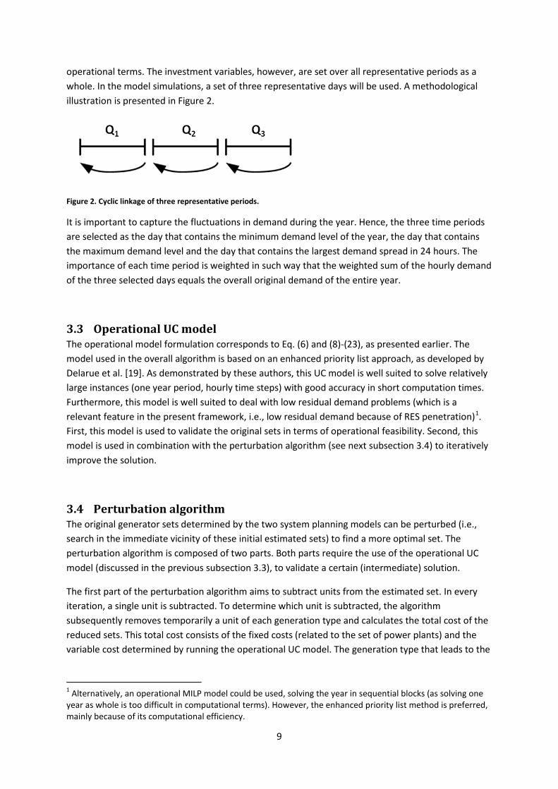
operational terms. The investment variables, however, are set over all representative periods as a whole. In the model simulations, a set of three representative days will be used. A methodological illustration is presented in Figure 2.
Figure 2. Cyclic linkage of three representative periods.
It is important to capture the fluctuations in demand during the year. Hence, the three time periods are selected as the day that contains the minimum demand level of the year, the day that contains the maximum demand level and the day that contains the largest demand spread in 24 hours. The importance of each time period is weighted in such way that the weighted sum of the hourly demand of the three selected days equals the overall original demand of the entire year.
3.3 Operational UC model The operational model formulation corresponds to Eq. (6) and (8)-(23), as presented earlier. The model used in the overall algorithm is based on an enhanced priority list approach, as developed by Delarue et al. [19]. As demonstrated by these authors, this UC model is well suited to solve relatively large instances (one year period, hourly time steps) with good accuracy in short computation times. Furthermore, this model is well suited to deal with low residual demand problems (which is a relevant feature in the present framework, i.e., low residual demand because of RES penetration)1. First, this model is used to validate the original sets in terms of operational feasibility. Second, this model is used in combination with the perturbation algorithm (see next subsection 3.4) to iteratively improve the solution.
3.4 Perturbation algorithm The original generator sets determined by the two system planning models can be perturbed (i.e., search in the immediate vicinity of these initial estimated sets) to find a more optimal set. The perturbation algorithm is composed of two parts. Both parts require the use of the operational UC model (discussed in the previous subsection 3.3), to validate a certain (intermediate) solution.
The first part of the perturbation algorithm aims to subtract units from the estimated set. In every iteration, a single unit is subtracted. To determine which unit is subtracted, the algorithm subsequently removes temporarily a unit of each generation type and calculates the total cost of the reduced sets. This total cost consists of the fixed costs (related to the set of power plants) and the variable cost determined by running the operational UC model. The generation type that leads to the
1 Alternatively, an operational MILP model could be used, solving the year in sequential blocks (as solving one year as whole is too difficult in computational terms). However, the enhanced priority list method is preferred, mainly because of its computational efficiency.

10
largest cost reduction when subtracted, is permanently removed from the set of generation units. A schematic overview is shown in Figure 3.
Figure 3. Schematic representation of the first part of the perturbation algorithm.
The first part of the algorithm is completed when no further cost reduction can be achieved by removing a generation unit. The second part of the algorithm is analogous to the first part. This time a unit is added in each iteration.
Note that when a unit is subtracted during an iteration, it is often not possible to serve the demand with the remaining generator set. Therefore, other units are simultaneously added when one unit is subtracted. The units that are added have a combined capacity which is less than the capacity of the subtracted unit. An analogous remark can be made for the second part of the algorithm, i.e., when adding a unit, it is usually possible to turn off a more expensive unit for the entire time horizon. In this case the adding of one unit will lead to the simultaneous removal of another unit.
4 Model simulations The developed model is applied to a methodological case study, optimizing the planning of an electricity generation system, under different wind deployment scenarios. The next subsection describes the input data, while the following subsection presents an overview of the model outcome. A third subsection discusses the performance of the different system planning models compared the overall algorithm. Finally, the fourth subsection focuses on the evolution of the system with increasing amounts of wind generation.
4.1 Data description
Estmated set
Subtract generatorof 1st type
Start set
Subtract generatorof 2nd type
Subtract generatorof nth type
Total cost 1st set
Total cost 2nd set
Total cost nth set
Select the set withsmallest cost
Smallest cost < start cost?
Start cost
Continue to secondpart of algorithm
Yes
No
Selected setbecomes start set

11
The demand profile is based on load-data from the Belgian transmission system operator Elia [20] from the year 2011. The magnitude is scaled and the resolution of the load-data is modified to obtain a demand profile with load values at hourly intervals and a maximum load of approximately 8 GW. The time horizon of the demand profile is one year. The reserve requirement is set at 5% of the demand, in both upward and downward direction.
The selected profile of electricity generated from wind energy is based on Belgian generation data from 2011. The generation data is obtained from Elia [21]. Analogously to the demand profile, the resolution of the generation profile is converted from quarter values to hourly values. The magnitude of the generation profile is varied linearly to create five different scenarios. The amount of wind capacity installed in each scenario ranges from minimum 0 MW (“0%” wind scenario) to maximum 4334 MW (“100%” wind scenario). This maximum amount of installed wind results in a residual demand with a minimum of 150 MW.
Table 1 displays a number of characteristics for every scenario, from 0% to 100% wind. The amount of installed wind capacity in each scenario is presented. The residual demand for each scenario is characterized by the minimum, maximum and average load. At last two key figures are displayed to quantify the volatility of the demand in each scenario. The first number is the maximum spread (i.e., the maximum demand minus the minimum demand) that occurs in a 24 hour time period. A second number given is the average diurnal spread relative to the annual peak demand, referred to as the average diurnal spread.
Table 1. Characteristics of the residual demand and wind profile of each scenario.
Scenario 0% 25% 50% 75% 100%
Wind cap [MW] 0 1083 2167 3250 4334
Min load [MW] 3786 3150 2254 1206 150
Max load [MW] 7881 7879 7877 7874 7872
Avg load [MW] 5712 5339 4965 4592 4219
Max 24h spread [MW] 2713 2991 3733 4535 5339
Average diurinal spread 20.98% 22.00% 24.47% 27.93% 31.97%
A set of five different generation technologies is selected to represent potential generating units. The economical characteristics of each generation technology are based on data obtained from [22]. The technical characteristics are based on data obtained from [23] and [24]. Note that these characteristics are purely methodological and intended to represent different types of generation technology (i.e., base, mid and peak load) and thus, are to be regarded as such.
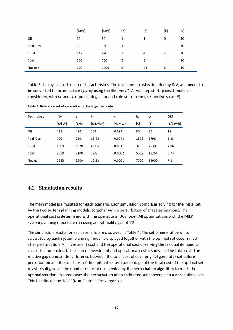
The technical data is shown Table 2. tcold represent the amount of hours after the minimum downtime from when it is assumed that the unit will make a cold start. A last characteristic given is LT, the assumed lifetime of each generator type.
Table 2. Reference set of generation technology: technical data.
Technology Pmin Pmax MUT MDT tcold LT
12
[MW] [MW] [h] [h] [h] [y]
Oil 10 50 1 1 0 30
Peak Gas 30 150 1 2 1 30
CCGT 147 420 2 4 2 30
Coal 300 750 5 8 4 30
Nuclear 600 1000 8 24 8 40
Table 3 displays all cost-related characteristics. The investment cost is denoted by INV, and needs to be converted to an annual cost fcr by using the lifetime LT. A two-step startup cost function is considered, with hc and cc representing a hot and cold startup cost, respectively (set P).
Table 3. Reference set of generation technology: cost data.
Technology INV a b c hc cc OM
[€/kW] [€/h] [€/MWh] [€/MWh2] [€] [€] [€/MWh]
Oil 461 450 104 0.034 30 60 18
Peak Gas 720 950 65.48 0.0043 1898 3796 5.38
CCGT 1069 1320 49.65 0.001 3765 7530 4.06
Coal 2539 2100 22.8 0.0002 5632 11264 8.73
Nuclear 5383 3500 12.33 0.0001 7500 15000 7.2
4.2 Simulation results
The main model is simulated for each scenario. Each simulation comprises solving for the initial set by the two system planning models, together with a perturbation of these estimations. The operational cost is determined with the operational UC model. All optimizations with the MILP system planning model are run using an optimality gap of 1%.
The simulation results for each scenario are displayed in Table 4. The set of generation units calculated by each system planning model is displayed together with the optimal set determined after perturbation. An investment cost and the operational cost of serving the residual demand is calculated for each set. The sum of investment and operational cost is shown as the total cost. The relative gap denotes the difference between the total cost of each original generator set before perturbation and the total cost of the optimal set as a percentage of the total cost of the optimal set. A last result given is the number of iterations needed by the perturbation algorithm to reach the optimal solution. In some cases the perturbation of an estimated set converges to a non-optimal set. This is indicated by 'NOC' (Non-Optimal Convergence).

13
Table 4. Simulation results for the different wind scenarios (0 – 100%). SC denotes the set of power plants obtained with the screening curve methodology, MILP denotes the MILP system planning model (representative days), while Optimal denotes the set obtained after perturbation.
wind scenario 0% 25% 50% model SC MILP Optimal SC MILP Optimal SC MILP Optimal
Oil [#] 14 5 20
20 7 25
23 8 28
Peak Gas [#] 3 0 3
3 2 3
4 1 2
CCGT [#] 2 2 2
2 2 2
2 2 2
Coal [#] 1 3 0
1 4 1
2 4 1
Nuclear [#] 6 5 6 6 4 5 6 4 5
Operational cost [M€] 1227.34 1276.43 1265.19
1137.13 1250.06 1217.07
1058.46 1147.7 1118.32
Investment cost [M€] 922.41 897.07 863.55
927.02 834.71 796.29
996.4 831.88 795
Total cost [M€] 2149.75 2173.51 2128.74 2064.16 2084.77 2013.36 2054.87 1979.58 1913.31
Relative gap 0.98% 2.06% 0.00%
2.46% 3.43% 0.00%
6.89% 3.35% 0.00%
Perturbation steps [#] 5 NOC - 4 NOC - 5 NOC -
wind scenario 75% 100% model SC MILP Optimal SC MILP Optimal Oil [#] 26 16 30
28 12 36
Peak Gas [#] 4 0 3
4 1 4 CCGT [#] 2 3 2
3 2 2
Coal [#] 2 5 2
2 9 3 Nuclear [#] 5 3 4 5 0 3 Operational cost [M€] 1017.09 1130.87 1098.01
955.1 1303.59 1096.21
Investment cost [M€] 864.13 778.29 729.03
880.64 614.03 666.14 Total cost [M€] 1881.22 1909.16 1827.04 1835.74 1917.61 1762.35 Relative gap 2.88% 4.30% 0.00%
4.00% 8.10% 0.00%
Perturbation steps [#] 6 NOC - NC NOC -
These results are now discussed, first in terms of modeling performance, and second focusing on the outcome, regarding the impact of increasing intermittent RES on the rest of the system.
4.3 Performance of the different planning models
The results presented in Table 4 are now further analyzed. A first question is whether the set of power plants obtained with a basic system planning model (that does not take into account detailed technical constraints (screening curve) or only considers a limited time frame (MILP)), is actually feasible to serve the load over the entire year, with technical constraints taken into account (solved with the operational model). As it turns out, the initial sets are feasible in operational terms in all simulations (both models, all wind scenarios). When comparing the initial sets of both models, it can be seen that the amount of generation capacity determined by the screening curve model (SC) is greater than the amount of capacity determined by the MILP model. This is explained by the fact that the screening curve model rounds up the optimal amount of generation capacity to convert the

14
amount of capacity to an amount of discrete generation units. A small amount of capacity needed can thereby lead to the installation of an entire generation unit2. Despite the higher installed capacity, the total cost of the screening curve model is in every wind scenario lower than the MILP model.
When using the initial sets of the two planning models in the perturbation algorithm, in every wind scenario the final solution obtained with the screening curve outperforms the solution obtained when starting from the MILP model. This best solution is denoted “optimal” and each time presented as third solution. The final solution obtained from the MILP after perturbation is 0.36%, 1.3%, 0.53%, 1.15% and 5.39% higher than the best solution (obtained from starting perturbation from the SC set), for the 0%, 25%, 50%, 75% and 100% wind scenario, respectively. There is further a trend of an increasing difference between the overall cost of the initially estimated sets and that of the optimal set, as wind power increases.
A note needs to be made on the perturbation of the initial set of the screening curve model in the 100% wind scenario. Perturbing this estimated set leads not to convergence. During an iteration of the perturbation process, a set was obtained, for which it was not possible to determine a feasible commitment schedule with. This is indicated as 'NC' (No Convergence) in Table 4. Hence, the initial set was modified in a heuristic manner, removing one CCGT unit and adding peak oil fired units instead. With this solution as start value for the perturbation algorithm, the optimal set was obtained. Perturbing the estimated set determined by the MILP system planning model did converge but again to a non-optimal set.
The numerical results show that the screening curve model provides a better estimation of the optimal generator set compared to the MILP system planning model. The screening curve model provides a quick estimation of the optimal set, but perturbation is always needed. The results obtained from the MILP system planning model are always far from the optimal generator set. Perturbing of these results thereby does not lead to the optimal set of generators. In addition the set estimated by the MILP model differs strongly for each scenario. This is explained by the fact that the MILP model makes its investment decision on a very limited amount of data.
As outlined in section 3.2, the MILP system planning model works with the days containing the maximum and minimum demand and a day with the largest demand spread. The relative importance of each representative day is incorporated through different weights in the objective function. This way, the minimum, maximum and average demand are equal for the whole demand and the representative profile (3 days). However, these numbers cannot characterize the entire demand profile. As an example, the relative average diurnal spread is computed for both the entire demand profile and the three representative days. This is an indication for the volatility of the demand. A number for each scenario is shown in Table 5. It is clear that the amount of volatility differs significantly. As other relevant characterizing parameters could be identified as well, it is not possible to capture all of these in the right proportion. Especially the variable profile of wind is difficult to
2 Another way to convert the continuous amount of generation capacity to a discrete number of units is to round one type of generation capacity to the nearest number of discrete units and add the difference in generation capacity obtained to the generation capacity of another type of technology. This method is examined, but the resulting generator set is generally not able to serve the demand. This method is therefore not further pursued.

15
capture in representative days, even more when combined with the fluctuating demand3. Hence, this indicates the necessity to consider both demand and RES on a time frame as large as possible (preferably the entire year). In this case, using 3 days clearly is insufficient to achieve an adequate representation. However, also when considering longer representative periods, this issue remains. Recall further that when increasing the number of periods, computation times will increase accordingly and hence, other assumptions might have to be made to ensure solvability.
Table 5. Indication of the difference in volatility between the entire demand profile and the representative days.
Scenario 0% 25% 50% 75% 100%
Entire demand profile 20.98% 22.00% 24.47% 27.93% 31.97%
Three days 22.31% 25.95% 31.02% 41.37% 47.04%
4.4 Evolution of the optimal generator set as a function of wind power deployment
The influence of the amount of wind capacity on the estimated and optimal sets of generation units is shown by Figure 4. The figure displays the amount of installed capacity per generation type, per system planning model and per scenario. The figure shows the estimated generator sets from the screening curve and the MILP system planning model together with the optimal set.
Figure 4. Installed capacity of different models for each scenario.
Figure 5 provides a more detailed illustration of the optimal generator set as a function of the wind capacity. It is clear that when more wind capacity is installed, the amount of base-load capacity 3 The original load as such could be characterized more easily, as it has typical diurnal, weekly and seasonal patterns.

16
reduces while the amount of mid-load and peak-load generation units increases. The total amount of installed capacity (excluding wind) remains approximately equal for all scenarios.
Figure 5. Installed capacity of optimal set for each scenario.
The replacement of base-load capacity by mid- and peak-load capacity in scenarios with more wind, is explained by two different effects. The first effect is an economic effect. An increase of installed wind capacity causes the total residual demand to decrease. In turn, this leads to a decrease of the total output of each generation unit. The decrease of generation output is unfavorable for base-load generation units as they are only economically preferable when their generation output is high.
The second effect is an operational effect. An increasing amount of installed wind capacity causes an increasing volatility of the residual demand. An increasing amount of flexible generation capacity is required to serve a demand with increasing volatility. This is again unfavorable for the base-load generation units, since their operational flexibility is more limited than the flexibility of a peak-load plant.
A comparison between two sets of generation capacity is made to examine the importance of both effects. The first set is the optimal set of generators, as determined by the developed methodology, incorporating operational constraints. In this case, both the economical and operational effect influence the amount of installed capacity as a function of the installed wind capacity. The second set is determined with the screening curve model without rounding the obtained solution to a discrete set of generation units. This implies that only the economic effect (reducing the demand) influences the amount of installed capacity in the second set. The installed generation capacity in each set as a function of the wind capacity is shown in Figure 6.

17
Figure 6. Installed capacity of un-rounded screening curve (SC) model, and optimal set, for each scenario.
For most scenarios, the amount of base load (nuclear) capacity replaced in the optimal set is approximately double the amount of replaced capacity in the screening curve set. This leads to the conclusion that both the economic and operational effect are important when determining the optimal set of generation units as a function of the installed wind capacity: (1) the deployment of RES reduces the residual load and hence creates a shift from base to mid and peak load; (2) this RES deployment also increases the volatility of the residual load, so this shift from base to peak load becomes even stronger.
5 Conclusion A first conclusion relates to the use of the screening curve model and the MILP system planning model as such. As they both provide solutions that are feasible also in operational terms, for cases with or without RES, in theory they can both be used for system planning. The screening curve methodology provides a good estimation of the optimal set and does so in the least amount of computation time. In addition, the perturbation generally converges to the optimal set. Only in case of 100% wind it occurs that the UC scheduling model employed by the perturbation algorithm could not determine a feasible UC schedule within reasonable calculation time. The MILP system planning model provides in general a worse initial estimation. This model takes by far the most time to determine an estimated set. The composition of each estimated set changes heavily for each scenario. This is because the model bases its investment decision on a very small part of the demand profile. A perturbation of the estimated set converges in general to a non-optimal set.
As is clear from the perturbation algorithm, taking into account operational constraints through an actual operational UC model affects the optimal solution. Hence, the basic system planning models can be used as such (providing feasible solutions), but need further adaptation to improve their performance (in achieving better solutions).
The second conclusion relates to the evolution of the optimal set in function of the amount of installed wind capacity. It is observed that the total amount of installed capacity (excluding wind) is

18
approximately equal for all scenarios. When more wind capacity is installed, a part of the base-load generation units is replaced by mid-load and peak-load generation units. This is explained by two effects. The first effect is an economic effect. An increase of installed wind capacity causes the total residual demand to decrease. A decrease in total residual demand leads to a decrease of the average generation output per generation unit. The decrease of generation output is unfavorable for base-load generation units as they are only economically preferable when their generation output is high. The second effect is an operational effect. An increasing amount of installed wind capacity causes an increase in the volatility of the residual demand. This leads to an increasing need for flexible generation units. This is again unfavorable for the base-load generation units, since their operation flexibility is limited compared to the flexibility of a peak-load generation unit. An examination of the simulation results lead to the conclusion that both effects have a significant impact on the composition of the optimal generator set.
Acknowledgements
E. Delarue is a research fellow of the Research Foundation – Flanders (FWO).
References
[1] Ortega-Vazquez MA, Kirschen DS. Assessing the impact of wind power generation on operating
costs. IEEE Transactions on Smart Grid. 2010;1:295-301.
[2] Restrepo JF, Galiana FD. Assessing the yearly impact of wind power through a new hybrid
deterministic/stochastic unit commitment. IEEE Transactions on Power Systems. 2011;26:401-10.
[3] Ummels BC, Gibescu M, Pelgrum E, Kling WL, Brand AJ. Impacts of wind power on thermal
generation unit commitment and dispatch. IEEE Transactions on Energy Conversion. 2007;22:44-51.
[4] Hobbs BF. Optimization methods for electric utility resource planning. European Journal of
Operational Research. 1995;83:1-20.
[5] Hobbs BF, Centolella P. Environmental policies and their effects on utility planning and
operations. Energy. 1995;20:255-71.
[6] Stoft S. Power System Economics. New York: Wiley; 2002.
[7] Hu Q, Huang G, Cai Y, Huang Y. Feasibility-based inexact fuzzy programming for electric power
generation systems planning under dual uncertainties. Applied Energy. 2011;88:4642-54.

19
[8] Pina A, Silva CA, Ferrão P. High-resolution modeling framework for planning electricity systems
with high penetration of renewables. Applied Energy. 2013;112:215-23.
[9] DeCesaro J, Porter K, Milligan M. Wind Energy and Power System Operations: A Review of Wind
Integration Studies to Date. The Electricity Journal. 2009;22:34-43.
[10] Denholm P, Hand M. Grid flexibility and storage required to achieve very high penetration of
variable renewable electricity. Energy Policy. 2011;39:1817-30.
[11] Holttinen H. Wind integration: experience, issues, and challenges. Wiley Interdisciplinary
Reviews: Energy and Environment. 2012;1:243-55.
[12] De Jonghe C, Delarue E, Belmans R, D’haeseleer W. Determining optimal electricity technology
mix with high level of wind power penetration. Applied Energy. 2011;88:2231-8.
[13] Maddaloni JD, Rowe AM, van Kooten GC. Wind integration into various generation mixtures.
Renewable Energy. 2009;34:807-14.
[14] Ma J, Kirschen DS, Belhomme R, Silva V. Optimizing the flexibility of a portfolio of generating
plants. Proc 2011 17th Power System Computation Conf(PSCC)2010. p. 22-6.
[15] Hawkes AD, Leach MA. Modelling high level system design and unit commitment for a microgrid.
Applied Energy. 2009;86:1253-65.
[16] Carrión M, Arroyo JM. A computationally efficient mixed-integer linear formulation for the
thermal unit commitment problem. IEEE Transactions on Power Systems. 2006;21:1371-8.
[17] Wood AJ, Wollenberg BF. Power generation, operation, and control: John Wiley & Sons; 2012.
[18] Nemhauser GL, Wolsey LA. Integer and combinatorial optimization: Wiley New York; 1988.
[19] Delarue E, Cattrysse D, D'haeseleer W. Enhanced priority list unit commitment method for
power systems with a high share of renewables. Electric Power Systems Research, submitted for
publication. 2013. Available at:
https://www.mech.kuleuven.be/en/tme/research/energy_environment/Pdf/wpen2013-07.pdf
[accessed July 2013].
[20] Elia. Grid data, demand. 2013. http://www.elia.be/nl/grid-data/data-download [accessed July
2013].

20
[21] Elia. Grid data, injected power from wind turbines. 2013. http://www.elia.be/nl/grid-
data/productie/windproductie [accessed July 2013].
[22] IEA/NEA. Projected Costs of Generating Electricity 2010 edition, International Eenrgy Agency /
Nuclear Energy Agency. Paris: OECD Publishing; 2010.
[23] Kazarlis SA, Bakirtzis A, Petridis V. A genetic algorithm solution to the unit commitment problem.
IEEE Transactions on Power Systems. 1996;11:83-92.
[24] Grigg C, Wong P, Albrecht P, Allan R, Bhavaraju M, Billinton R, et al. The IEEE reliability test
system-1996. A report prepared by the reliability test system task force of the application of
probability methods subcommittee. IEEE Transactions on Power Systems. 1999;14:1010-20.