Accepted Manuscript

Finite volume solvers and Moving Least-Squares approximations for the com‐

pressible Navier-Stokes equations on unstructured grids

Luis Cueto-Felgueroso, Ignasi Colominas, Xesús Nogueira, Fermín Navarrina,

Manuel Casteleiro

PII: S0045-7825(07)00248-4

DOI: 10.1016/j.cma.2007.06.003

Reference: CMA 8347

To appear in: Comput. Methods Appl. Mech. Engrg.

Accepted Date: 11 June 2007

Please cite this article as: L. Cueto-Felgueroso, I. Colominas, X. Nogueira, F. Navarrina, M. Casteleiro, Finite

volume solvers and Moving Least-Squares approximations for the compressible Navier-Stokes equations on

unstructured grids, Comput. Methods Appl. Mech. Engrg. (2007), doi: 10.1016/j.cma.2007.06.003

This is a PDF file of an unedited manuscript that has been accepted for publication. As a service to our customers

we are providing this early version of the manuscript. The manuscript will undergo copyediting, typesetting, and

review of the resulting proof before it is published in its final form. Please note that during the production process

errors may be discovered which could affect the content, and all legal disclaimers that apply to the journal pertain.

ACCEPTED MANUSCRIPT

Finite volume solvers and Moving

Least-Squares approximations for the

compressible Navier-Stokes equations on

unstructured grids

Luis Cueto-Felgueroso a,b, Ignasi Colominas b,∗,Xesus Nogueira b, Fermın Navarrina b and Manuel Casteleiro b

aAerospace Computational Design LaboratoryDepartment of Aeronautics and Astronautics

Massachusetts Institute of Technology77 Massachusetts Avenue, Cambridge MA 02139, USAbGroup of Numerical Methods in Engineering, GMNI

Dept. of Applied Mathematics, School of Civil EngineeringUniversidad de La Coruna

Campus de Elvina, 15071 La Coruna, Spain

Abstract

This paper explores the approximation power of Moving Least-Squares (MLS) ap-proximations in the context of higher order finite volume schemes on unstructuredgrids. The scope of the application of MLS is threefold: 1) computation of highorder derivatives of the field variables for a Godunov-type approach to hyperbolicproblems or terms of hyperbolic character, 2) direct reconstruction of the fluxes atcell edges, for elliptic problems or terms of elliptic character, and 3) multiresolutionshock detection and selective limiting. A major advantage of the proposed method-ology over the most popular existing higher order methods is related to the viscousdiscretization. The use of MLS approximations allows the direct reconstruction ofhigh order viscous fluxes using quite compact stencils, and without introducing newdegrees of freedom, which results in a significant reduction in storage and workload.A selective limiting procedure is proposed, based on the multiresolution proper-ties of the MLS approximants, which allows to switch off the limiters in smoothregions of the flow. Accuracy tests show that the proposed method achieves theexpected convergence rates. Representative simulations show that the methodologyis applicable to problems of engineering interest.

Key words: Compressible flow, Finite volume method, High-resolution methods,High-order methods, Moving Least-Squares, Unstructured grids.

Preprint submitted to Elsevier Science 13 June 2007

ACCEPTED MANUSCRIPT

1 Introduction

This work is motivated by the question about whether piecewise polynomialapproximations are the best option for the construction of higher order Navier-Stokes solvers on unstructured grids. By this we refer to schemes that, eitherwithin the finite element framework (such as Discontinuous Galerkin methods[1]), or through suitable cell subdivisions (such as the so-called Spectral Vol-ume method [2]), create new degrees of freedom inside each cell and use themto construct piecewise polynomial interpolants. The most important advan-tage of this kind of approaches is that, under certain conditions, the high orderinterpolation/reconstruction can be formulated in a quite robust and generalsetting (particularly in the case of DG). Painful viscous discretizations, whereadditional degrees of freedom must be introduced and solved for, the necessar-ily high order grids required and, in the case of higher order DG, the absence ofrobust and accurate shock-capturing techniques, are major drawbacks of thisapproach. By accurate shock-capturing we mean shock resolutions comparableto typical second-order finite volume or residual distribution schemes.

Of course, having the general approximation framework of the finite elementmethod makes DG the “safe” path, and it is understandable that many authorsmay be willing to pay the price of very high cost and “robustness uncertainty”in order to follow it. This study is aimed at showing that, perhaps only for themore adventurous, there may be other less safe, but maybe better, options.

Originally devised for data processing and surface generation [3], MovingLeast-Squares (MLS) became very popular within the meshfree community,being widely used, both in eulerian and lagrangian formulations, in order toprovide spatial approximation. The characteristics of Moving Least-Squaresand reproducing kernel methods have been extensively analyzed, both fromtheoretical and purely numerical approaches [4–8]. This class of approximationmethods is particularly well suited for the reconstruction of a given functionand its successive derivatives from scattered, pointwise data. This fact sug-gested the incorporation of MLS approximants into finite volume methods onunstructured grids [9], somewhat providing a kind of “shape functions” forunstructured-grid finite volume solvers.

The scope of the application of MLS to develop higher order finite volumeschemes, as we understand it, is threefold: 1) computation of high order deriva-tives of the field variables for a Godunov-type approach to hyperbolic problemsor terms of hyperbolic character, 2) direct reconstruction of the fluxes at celledges, for elliptic problems or terms of elliptic character, and 3) multiresolu-

∗ Correspondence to: E.T.S. de Ingenieros de Caminos, Canales y Puertos, Univer-sidad de La Coruna, Campus de Elvina, 15071 La Coruna, Spain.

Email address: icolominas@udc.es (Ignasi Colominas).

2

ACCEPTED MANUSCRIPT

tion shock detection and selective limiting.

Quite the opposite to most existing high order finite volume schemes, our ap-proach is “top-down”. Firstly, instead of adopting the cell-average framework,we work with pointwise values of the conserved variables, associated to thecell-centroids. Furthermore, our spatial representation, which is provided bythe MLS approximants, is continuous and already high order accurate. Notethat the discretization of elliptic problems is straightforward within this frame-work. In order to deal with convection-dominated problems, and to apply theusual finite volume technology for hyperbolic terms, we break our continuousrepresentation locally (inside each cell), by means of Taylor series expansions.The resulting scheme has the flavor of a Godunov-type method, but the accu-rate and clear discretization of elliptic terms is a crucial advantage over mostexisting approaches.

The strategy adopted for convection terms follows the ideas of the generalizedGodunov method [10–12], performing piecewise polynomial reconstructions ofthe field variables inside each cell, and subsequently using those reconstructedvariables as input data for a numerical flux function [12–15]. In practice, theconstruction of very high order schemes of this kind has been severely lim-ited by the absence of robust approximation techniques, capable of providingaccurate estimates of the succesive derivatives of the field variables on unstruc-tured grids. Thus, the concept of high-order scheme is most frequently used inthe literature in reference to formally second order schemes (piecewise linearreconstruction). We believe the use of powerful approximation techniques likeMLS may open new perspectives for this kind of schemes.

As mentioned above, a major advantage of the proposed methodology overthe most popular existing higher order methods is related to the viscous dis-cretization. The use of MLS approximations allows the direct reconstructionof high order viscous fluxes using quite compact stencils, and without intro-ducing new degrees of freedom. This approach is conceptually similar to thesuccessful second-order Multi-Point Flux Approximation (MPFA) methodsdeveloped by the petroleum engineering community [18].

Even though well behaved limiters for second order schemes have been de-veloped, the question for higher order reconstructions is far from being clear.Therefore, selective shock-capturing is a critical issue in this context. If thelimiters are active over the whole domain, their deleterious effect on higherorder derivatives results into a partial (or, quite frequently, complete) loss ofthe higher order accuracy of the reconstruction in smooth regions of the flow,virtually taking the method back to second order.

A selective limiting procedure is proposed, based on the multiresolution prop-erties of the MLS approximants [19], which allows to switch off the limiters in

3

ACCEPTED MANUSCRIPT

smooth regions of the flow. Note that the concept of “smooth region” itself isstrongly related to the approximation being used, and hence the convenienceof an indicator that is of the same order and nature as the approximants. Insome sense, this procedure can be regarded as an unstructured grid general-ization of the wavelet-based selective filtering proposed by Sjogreen and Yeefor finite differences [20].

The outline of the paper is as follows. Section 2 presents the model equationsand basic numerical scheme. Section 3 is a brief introduction to Moving LeastSquares Reproducing Kernel approximation methods, which is completed withsome practical implementation issues presented in section 4. Accuracy testsand representative simulations are exposed in sections 5 and 6 and, finally,our main conclusions are drawn in section 7.

2 Mathematical model and basic finite volume scheme

2.1 Governing equations.

The compressible Navier-Stokes equations for two-dimensional flow, writtenin cartesian coordinates and in the absence of source terms, can be cast inconservative form as

∂UUUUUUUUUUUUUU

∂t+

∂(FFFFFFFFFFFFFF x − FFFFFFFFFFFFFF Vx )

∂x+

∂(FFFFFFFFFFFFFF y − FFFFFFFFFFFFFF Vy )

∂y= 00000000000000 (1)

being

UUUUUUUUUUUUUU =

ρρuρvρE

, FFFFFFFFFFFFFF x =

ρuρu2 + p

ρuvρuH

, FFFFFFFFFFFFFF y =

ρvρuv

ρv2 + pρvH

(2)

the conserved variables and inviscid fluxes, respectively, and

FFFFFFFFFFFFFF Vx =

0τxx

τxy

uτxx + vτxy − qx

, FFFFFFFFFFFFFF V

y =

0τxy

τyy

uτxy + vτyy − qy

(3)

4

ACCEPTED MANUSCRIPT

the viscous fluxes. In the above expressions, ρ denotes density, p pressure andvvvvvvvvvvvvvv = (u, v) is the velocity vector. The total energy and enthalpy are given by

ρE = ρe +1

2ρ vvvvvvvvvvvvvv · vvvvvvvvvvvvvv, H = E +

p

ρ(4)

where e is the specific internal energy. The viscous stresses are modelled as

τxx = 2µ∂u

∂x− 2

3µ

(∂u

∂x+

∂v

∂y

)

τyy = 2µ∂v

∂y− 2

3µ

(∂u

∂x+

∂v

∂y

)

τxy = µ

(∂u

∂y+

∂v

∂x

)(5)

where µ is the viscosity. The heat fluxes are assumed to be represented byFourier’s law

qx = −λ∂T

∂x, qy = −λ

∂T

∂y(6)

where T denotes temperature, λ = cpµ/Pr is the thermal conductivity, cp

the specific heat at constant temperature (cp = 1003.5 for air) and Pr is thePrandtl number (Pr = 0.72 for air). The equation of state and temperaturefor an ideal gas can be written as

p = (γ − 1)(ρE − 1

2ρvvvvvvvvvvvvvv · vvvvvvvvvvvvvv), T =

1

cv

p

ρ(γ − 1)(7)

where cv is the specific heat at constant volume (cv = 716.5 for air) and γ =cp

cvis the ratio of specific heats (γ = 1.4 for air). The speed of sound is given by

c =√

γp/ρ (8)

and the dynamic viscosity µ is assumed to be related to the temperatureaccording to Sutherland’s law

µ = µ∞T + S0

T∞ + S0

(T

T∞

)1.5

(9)

where µ∞ and T∞ denote freestream viscosity and temperature, respectively,and S0 = 110.4 K is an experimental constant [21].

5

ACCEPTED MANUSCRIPT

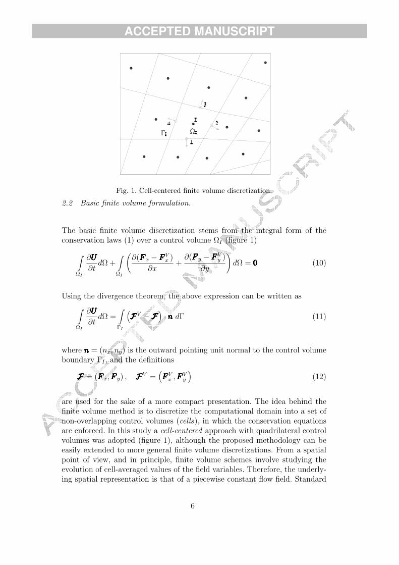
Fig. 1. Cell-centered finite volume discretization.

2.2 Basic finite volume formulation.

The basic finite volume discretization stems from the integral form of theconservation laws (1) over a control volume ΩI (figure 1)

∫

ΩI

∂UUUUUUUUUUUUUU

∂tdΩ +

∫

ΩI

(∂(FFFFFFFFFFFFFF x − FFFFFFFFFFFFFF V

x )

∂x+

∂(FFFFFFFFFFFFFF y − FFFFFFFFFFFFFF Vy )

∂y

)dΩ = 00000000000000 (10)

Using the divergence theorem, the above expression can be written as

∫

ΩI

∂UUUUUUUUUUUUUU

∂tdΩ =

∫

ΓI

(FFFFFFFFFFFFFFV −FFFFFFFFFFFFFF

)· nnnnnnnnnnnnnn dΓ (11)

where nnnnnnnnnnnnnn = (nx, ny) is the outward pointing unit normal to the control volumeboundary ΓI , and the definitions

FFFFFFFFFFFFFF = (FFFFFFFFFFFFFF x, FFFFFFFFFFFFFF y) , FFFFFFFFFFFFFFV =(FFFFFFFFFFFFFF V

x , FFFFFFFFFFFFFF Vy

)(12)

are used for the sake of a more compact presentation. The idea behind thefinite volume method is to discretize the computational domain into a set ofnon-overlapping control volumes (cells), in which the conservation equationsare enforced. In this study a cell-centered approach with quadrilateral controlvolumes was adopted (figure 1), although the proposed methodology can beeasily extended to more general finite volume discretizations. From a spatialpoint of view, and in principle, finite volume schemes involve studying theevolution of cell-averaged values of the field variables. Therefore, the underly-ing spatial representation is that of a piecewise constant flow field. Standard

6

ACCEPTED MANUSCRIPT

high order schemes are constructed through the substitution of this piece-wise constant representation for a piecewise continuous (usually polynomial)reconstruction of the flow variables inside each cell. In addition, and due tothe fact that the reconstructed fields are still discontinuous across interfaces,special care must be paid to the discretization of the viscous fluxes, which arefunctions of the conserved variables, but also of their gradients. According tothis description, most existing high order finite volume schemes work withina cell-average setting, and proceed “bottom-up”.

Our approach is somewhat the opposite. Firstly, instead of adopting the cell-average framework, we work with pointwise values of the conserved variables,associated to the cell-centroids. Furthermore, our spatial representation, whichis provided by the Moving Least-Squares (MLS) approximants, is continu-ous and already high order accurate. Note that the discretization of ellip-tic problems is straightforward within this framework. In order to deal withconvection-dominated problems, and to apply the usual finite volume tech-nology for hyperbolic terms, we break our continuous representation locally(inside each cell), by means of Taylor series expansions. In this sense, weproceed “top-down”. The resulting scheme has the flavor of a Godunov-typemethod, but the accurate and clear discretization of elliptic terms is a crucialadvantage of our scheme. More details of the proposed formulation can befound in [22].

Adopting the numerical method of lines, focusing on a control volume I, andassuming that suitable approximations to the inviscid and viscous fluxes areavailable at a set of quadrature points at each edge, the semi-discrete versionof (11) reads

AIdUUUUUUUUUUUUUU I

dt=

nedgeI∑

iedge=1

ngauI∑

igau=1

[(FFFFFFFFFFFFFFV −FFFFFFFFFFFFFF

)· nnnnnnnnnnnnnn

]igau

Wigau (13)

where AI is the area of cell I, nedgeI the number of cell edges, ngauI thenumber of Gauss quadrature points on each edge, Wigau denotes a quadratureweight and UUUUUUUUUUUUUU I represents, either the average value of UUUUUUUUUUUUUU over the cell I (cell-average approach), or the pointwise value of UUUUUUUUUUUUUU at the centroid of the cell I.In this latter case, the presence of AI instead of a consistent mass matrixassumes that a mass-lumping has been performed.

It is critical in the development of robust high order schemes for the Navier-Stokes equations to acknowledge the distinct nature of the inviscid and viscousfluxes. The former is of hyperbolic character, whereas the later is of ellipticcharacter. It is widely accepted that the most powerful schemes for hyper-bolic problems are those that take into account, in one way or another, theunderlying wave structure of the equations. In the finite volume context, this

7

ACCEPTED MANUSCRIPT

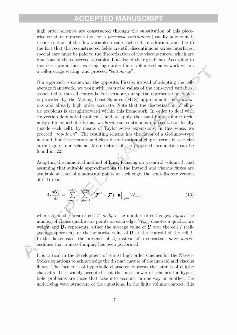
can be achieved by using upwind numerical flux functions, that take as inputvariables the states on either side of each interface, and return a single nu-merical flux. First order schemes use the cell-average values of the variableson each side of the interface as left and right states, whereas higher orderschemes use reconstructed ones, obtained from a certain extrapolation proce-dure. These ideas are in the basis of the generalized Godunov scheme [10–12],whose implementation involves three major steps in the explicit case:

• Development of piecewise continuous (usually polynomial) reconstruc-tions of the flow variables inside each control volume, using either cell-averaged or pointwise information from neighbour cells. In our case, weuse the point values of the variables at the cell centroids. The resultingspatial representation is still discontinuous across interfaces. The pres-ence of discontinuities or steep gradients in the solution may require theuse of some limiting strategy.

• Evaluation of fluxes at cell edges. The extrapolated left (+) and right(−) states at each edge integration point are used as input data for anapproximate Riemann solver (figure 2).

• Solution advancement, using appropriate time stepping algorithms.

Viscous terms pose a major problem for methods that use piecewise poly-nomial approximations. Second-order schemes often use the average of thederivatives of the flow variables on either side of the interface to compute theviscous fluxes. Unfortunately, higher order discretizations of elliptic equationsor viscous terms cannot follow this path. One alternative is to decompose theoriginal second-order system into a first order one, with the consequent intro-duction of additional degrees of freedom. Another option, and the one thatwill be adopted in this study, is to perform a reconstruction of the viscousfluxes using information from neighbouring cells. This approach is sometimesthought to require large stencils, therefore being less efficient in practice. It isone of the objectives of this study to show that, with the reconstruction tech-nique proposed, very competitive and efficient schemes for elliptic problemscan be devised via multi-point reconstruction.

3 Moving Least Squares Reproducing Kernel approximations

3.1 General formulation.

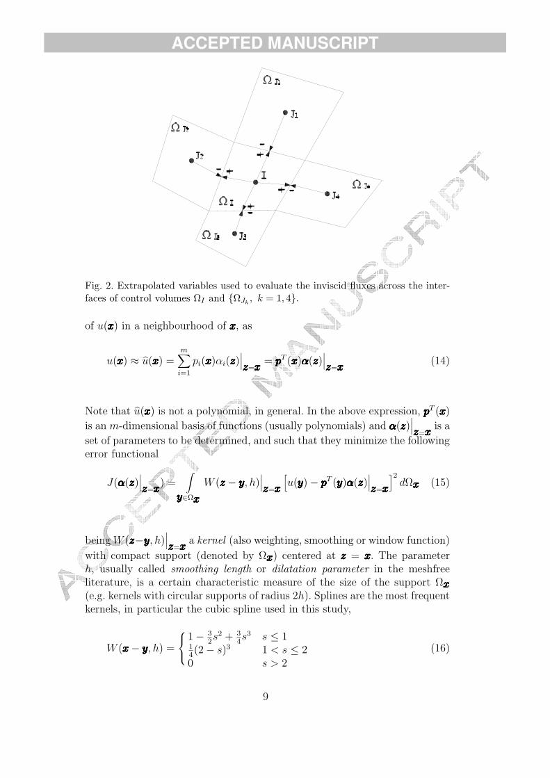
Consider a function u(xxxxxxxxxxxxxx) defined in a domain Ω. Moving Least-Squares (MLS)approximate u(xxxxxxxxxxxxxx), at a given point xxxxxxxxxxxxxx, through a weighted least-squares fitting

8

ACCEPTED MANUSCRIPT

Fig. 2. Extrapolated variables used to evaluate the inviscid fluxes across the inter-faces of control volumes ΩI and ΩJk

, k = 1, 4.

of u(xxxxxxxxxxxxxx) in a neighbourhood of xxxxxxxxxxxxxx, as

u(xxxxxxxxxxxxxx) ≈ u(xxxxxxxxxxxxxx) =m∑

i=1

pi(xxxxxxxxxxxxxx)αi(zzzzzzzzzzzzzz)∣∣∣zzzzzzzzzzzzzz=xxxxxxxxxxxxxx

= ppppppppppppppT (xxxxxxxxxxxxxx)αααααααααααααα(zzzzzzzzzzzzzz)∣∣∣zzzzzzzzzzzzzz=xxxxxxxxxxxxxx

(14)

Note that u(xxxxxxxxxxxxxx) is not a polynomial, in general. In the above expression, ppppppppppppppT (xxxxxxxxxxxxxx)

is an m-dimensional basis of functions (usually polynomials) and αααααααααααααα(zzzzzzzzzzzzzz)∣∣∣zzzzzzzzzzzzzz=xxxxxxxxxxxxxx

is a

set of parameters to be determined, and such that they minimize the followingerror functional

J(αααααααααααααα(zzzzzzzzzzzzzz)∣∣∣zzzzzzzzzzzzzz=xxxxxxxxxxxxxx

) =∫

yyyyyyyyyyyyyy∈Ωxxxxxxxxxxxxxx

W (zzzzzzzzzzzzzz − yyyyyyyyyyyyyy, h)∣∣∣zzzzzzzzzzzzzz=xxxxxxxxxxxxxx

[u(yyyyyyyyyyyyyy)− ppppppppppppppT (yyyyyyyyyyyyyy)αααααααααααααα(zzzzzzzzzzzzzz)

∣∣∣zzzzzzzzzzzzzz=xxxxxxxxxxxxxx

]2dΩxxxxxxxxxxxxxx (15)

being W (zzzzzzzzzzzzzz−yyyyyyyyyyyyyy, h)∣∣∣zzzzzzzzzzzzzz=xxxxxxxxxxxxxx

a kernel (also weighting, smoothing or window function)

with compact support (denoted by Ωxxxxxxxxxxxxxx) centered at zzzzzzzzzzzzzz = xxxxxxxxxxxxxx. The parameterh, usually called smoothing length or dilatation parameter in the meshfreeliterature, is a certain characteristic measure of the size of the support Ωxxxxxxxxxxxxxx(e.g. kernels with circular supports of radius 2h). Splines are the most frequentkernels, in particular the cubic spline used in this study,

W (xxxxxxxxxxxxxx− yyyyyyyyyyyyyy, h) =

1− 32s2 + 3

4s3 s ≤ 1

14(2− s)3 1 < s ≤ 2

0 s > 2

(16)

9

ACCEPTED MANUSCRIPT

where s =|xxxxxxxxxxxxxx− yyyyyyyyyyyyyy|

h. In practice, the minimization of (15) provides a means to

approximate or reconstruct u(xxxxxxxxxxxxxx), at any point xxxxxxxxxxxxxx ∈ Ω, from its pointwise valueat a number of scattered locations in Ω, which are often called particles ornodes .

The integral in (15) is evaluated using nodal integration and, given the com-pact support of the kernel, only those nodes inside Ωxxxxxxxxxxxxxx are involved as quadra-ture points. After some algebra, the set of parameters αααααααααααααα that minimize thefunctional J are obtained as

αααααααααααααα(zzzzzzzzzzzzzz)∣∣∣zzzzzzzzzzzzzz=xxxxxxxxxxxxxx

= MMMMMMMMMMMMMM−1(xxxxxxxxxxxxxx)PPPPPPPPPPPPPPΩxxxxxxxxxxxxxxWWWWWWWWWWWWWW V (xxxxxxxxxxxxxx)uuuuuuuuuuuuuuΩxxxxxxxxxxxxxx (17)

where the vector uuuuuuuuuuuuuuΩxxxxxxxxxxxxxx contains the pointwise values of the function to bereproduced, u (xxxxxxxxxxxxxx), at the nxxxxxxxxxxxxxx particles inside Ωxxxxxxxxxxxxxx (figure 3)

uuuuuuuuuuuuuuΩxxxxxxxxxxxxxx =(u(xxxxxxxxxxxxxx1) u(xxxxxxxxxxxxxx2) · · · u(xxxxxxxxxxxxxxnxxxxxxxxxxxxxx)

)T(18)

The moment matrix, M, which is an (m × m) matrix, is given by M(xxxxxxxxxxxxxx) =PΩxxxxxxxxxxxxxxWV(xxxxxxxxxxxxxx)PT

Ωxxxxxxxxxxxxxx , and the matrices PΩxxxxxxxxxxxxxx and WV(xxxxxxxxxxxxxx), whose dimensions are,

respectively, (m× nxxxxxxxxxxxxxx) and (nxxxxxxxxxxxxxx × nxxxxxxxxxxxxxx), can be obtained as

PPPPPPPPPPPPPPΩxxxxxxxxxxxxxx = (pppppppppppppp(xxxxxxxxxxxxxx1) pppppppppppppp(xxxxxxxxxxxxxx2) · · · pppppppppppppp(xxxxxxxxxxxxxxnxxxxxxxxxxxxxx) ) (19)

WV(xxxxxxxxxxxxxx) = diag Wi(xxxxxxxxxxxxxx− xxxxxxxxxxxxxxi)Vi , i = 1, . . . , nxxxxxxxxxxxxxx (20)

Complete details can be found in [4,5]. In the above equations, Vi and xxxxxxxxxxxxxxi

denote, respectively, the tributary volume (used as quadrature weight) andcoordinates associated to node i. Note that the tributary volumes of the neigh-bouring nodes are included in matrix WV, obtaining an MLS version of theReproducing Kernel Particle Method [4]. Otherwise, we can use W instead ofWV

W(xxxxxxxxxxxxxx) = diag Wi(xxxxxxxxxxxxxx− xxxxxxxxxxxxxxi) , i = 1, . . . , nxxxxxxxxxxxxxx (21)

which corresponds to the classical MLS approximation (in the nodal integra-tion of the functional (15), the same quadrature weight is associated to allnodes). Introducing (17) in (14), the interpolation structure can be identifiedas

u(xxxxxxxxxxxxxx) = ppppppppppppppT (xxxxxxxxxxxxxx)MMMMMMMMMMMMMM−1(xxxxxxxxxxxxxx)PPPPPPPPPPPPPPΩxxxxxxxxxxxxxxWWWWWWWWWWWWWW (xxxxxxxxxxxxxx)uuuuuuuuuuuuuuΩxxxxxxxxxxxxxx = NNNNNNNNNNNNNNT (xxxxxxxxxxxxxx)uuuuuuuuuuuuuuΩxxxxxxxxxxxxxx =nxxxxxxxxxxxxxx∑

j=1

Nj(xxxxxxxxxxxxxx)uj (22)

10

ACCEPTED MANUSCRIPT

In analogy to finite elements, the approximation was written in terms of theMLS “shape functions”

NNNNNNNNNNNNNNT (xxxxxxxxxxxxxx) = ppppppppppppppT (xxxxxxxxxxxxxx)MMMMMMMMMMMMMM−1(xxxxxxxxxxxxxx)PPPPPPPPPPPPPPΩxxxxxxxxxxxxxxWWWWWWWWWWWWWW (xxxxxxxxxxxxxx) (23)

where Nj(xxxxxxxxxxxxxx) can be seen as the shape function associated to particle j. Thefunctional basis pppppppppppppp(xxxxxxxxxxxxxx) is strongly related to the accuracy of the MLS fit. The-ory and numerical evidence [7] show that, for a pth order MLS fit (pth ordercomplete polynomial basis) and general, irregularly spaced points, the nomi-nal order of accuracy for the approximation of a sth order gradient is roughly(p− s+1). In general, any linear combination of the functions included in thebasis is exactly reproduced by the MLS approximation.

Fig. 3. Meshfree approximation: general scheme. Support for reconstruction at P.

In 2D, the p = 2 basis reads

pppppppppppppp(xxxxxxxxxxxxxx) =(1 x1 x2 x1x2 x2

1 x22

)T(24)

and the p = 3 basis is given by

pppppppppppppp(xxxxxxxxxxxxxx) =(1 x1 x2 x1x2 x2

1 x22 x2

1x2 x1x22 x3

1 x32

)T(25)

In the above expression, (x1, x2) denotes the cartesian coordinates of xxxxxxxxxxxxxx. Toimprove the conditioning of the moment matrix, it is most frequent to usescaled and locally defined monomials in the basis. Thus, if the shape functionswere to be evaluated at a certain point xxxxxxxxxxxxxxI , the basis would be of the formpppppppppppppp(xxxxxxxxxxxxxx−xxxxxxxxxxxxxxI

h), instead of pppppppppppppp(xxxxxxxxxxxxxx). With this transformation, the MLS shape functions

read

NNNNNNNNNNNNNNT (xxxxxxxxxxxxxxI) = ppppppppppppppT (00000000000000)CCCCCCCCCCCCCC(xxxxxxxxxxxxxxI) = ppppppppppppppT (00000000000000)MMMMMMMMMMMMMM−1(xxxxxxxxxxxxxxI)PPPPPPPPPPPPPPΩxxxxxxxxxxxxxxIWWWWWWWWWWWWWW (xxxxxxxxxxxxxxI) (26)

11

ACCEPTED MANUSCRIPT

where CCCCCCCCCCCCCC(xxxxxxxxxxxxxx) was defined as

CCCCCCCCCCCCCC(xxxxxxxxxxxxxx) = MMMMMMMMMMMMMM−1(xxxxxxxxxxxxxx)PPPPPPPPPPPPPPΩxxxxxxxxxxxxxxWWWWWWWWWWWWWW (xxxxxxxxxxxxxx) (27)

The approximate derivatives of u (xxxxxxxxxxxxxx) can be expressed in terms of the deriva-tives of the MLS shape functions, which are functions of the derivatives of thepolynomial basis pppppppppppppp(xxxxxxxxxxxxxx−xxxxxxxxxxxxxxI

h) and the derivatives of CCCCCCCCCCCCCC(xxxxxxxxxxxxxx) [9,23,24].

The first order derivatives of the shape functions are computed in this study asfull MLS derivatives, whereas second and third order derivatives are approxi-mated by the diffuse ones. In the diffuse approach, the succesive derivatives ofCCCCCCCCCCCCCC(xxxxxxxxxxxxxx) are neglected. Note that the diffuse derivatives of the shape functions arereadily obtained once the matrix CCCCCCCCCCCCCC(xxxxxxxxxxxxxx) is computed. Although this approachgreatly simplifies the presentation and implementation of the MLS approxi-mants, problems with rough grids may require the use of full derivatives.

More details of the MLS procedure used in this paper can be found in [9,23].

3.2 Computational aspects.

The MLS shape functions are data independent and, therefore, for fixed gridsthey need to be computed only once at the preprocessing phase. Note againthat the reconstructed function is not a polynomial , even in the case when thebasis of functions comprises only polynomials.

The evaluation of the shape functions at a given point involves a series ofmatrix operations, the most expensive of them being the inversion of themoment matrix MMMMMMMMMMMMMM . The size of this matrix is m×m, where m is the dimensionof the basis pppppppppppppp(xxxxxxxxxxxxxx). Note that the size of MMMMMMMMMMMMMM does not depend on the number ofneighbours in the cloud of the evaluation point.

In order to prevent the matrix MMMMMMMMMMMMMM from being singular or ill-conditioned, thecloud of neighbours should fulfill certain “good neighbourhood” requirements.Thus, if the number of neighbours is less than m (the number of functionsin the basis), MMMMMMMMMMMMMM becomes singular. Nevertheless, the approximation couldbe poor if MMMMMMMMMMMMMM is severely ill-conditioned, so it is convenient to use a numberof neighbours slightly above the minimum, and with the information comingfrom as many directions as possible. For rough grids it may be necessary to useanisotropic kernels [22]. The definition of the cloud (the MLS stencil) for eachevaluation point is an important issue that will be addressed in sections 4.2and 4.3. The selection process must be suitable for general unstructured grids,and the stencil should be as compact as possible for the sake of computationalefficiency and physical meaning.

12

ACCEPTED MANUSCRIPT

Once the cloud of neighbour centroids has been determined, the smoothinglength h for isotropic kernels (radial weighting) is set to be proportional tothe maximum distance between the evaluation point xxxxxxxxxxxxxxI and its neighours, as

h = k max (‖xxxxxxxxxxxxxxj − xxxxxxxxxxxxxxI‖) (28)

Values of k around 0.6–0.7 seem to be adequate (recall that, using radialweighting, the support of the kernel expands over a circle of radius 2h).

3.3 Moving Least Squares vs. Piecewise Polynomial interpolation.

Most existing higher order schemes are based on piecewise polynomial ap-proximations, which are obtained either within the finite element framework(consider the Discontinuous Galerkin method [1]), or using some suitable formof cell subdivision (such as the so-called Spectral Volume method [2]). Follow-ing this approach, higher order accuracy is achieved by creating new degrees offreedom inside each cell, which are used to construct an interpolating polyno-mial. This piecewise polynomial interpolation is discontinuous across elementinterfaces, a feature that is quite convenient in terms of the stability and com-pactness of the scheme for hyperbolic problems, but also quite inconvenientin terms of the efficiency of the scheme for equations and terms of ellipticcharacter. The way Moving Least Squares approximations work is rather dif-ferent, and this section is aimed at shedding some light on its advantages andshortcomings.

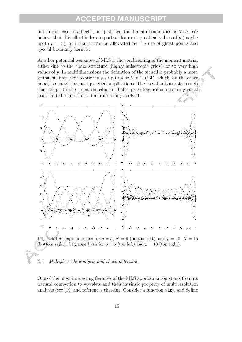
Even though the MLS approximants will be later used in a “moving” (cen-tered) sense, figures 4 and 5 present some examples of MLS shape functionscomputed in an “element” sense. By this we mean that, in order to computethe set of p-complete MLS shape functions associated to N points on [−1, +1],the cloud for each point comprises all the N points, instead of using compactsupports. This may be useful to give a flavour of the structure of the shapefunctions, and to have a first comparison to the Lagrange basis.

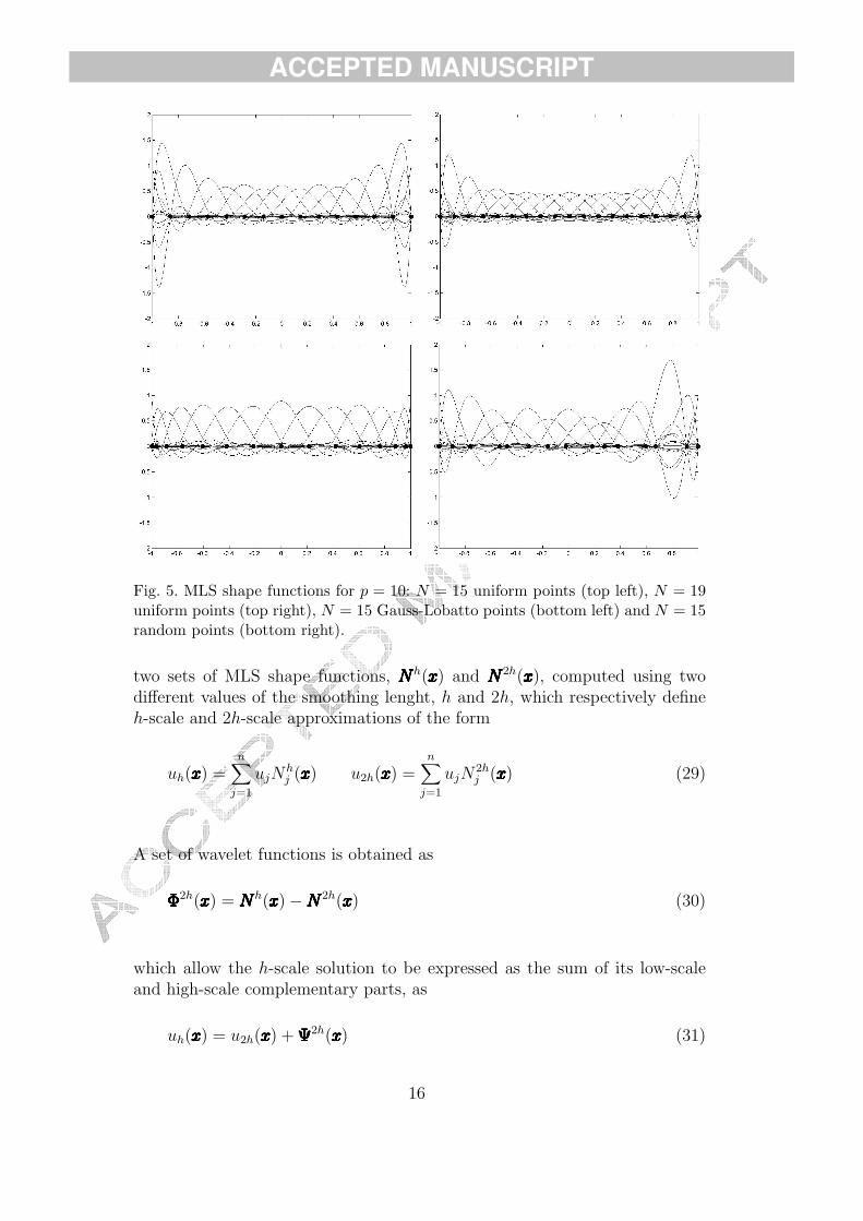
Figure 4 presents the computed shape functions for p = 5, N = 9 (bottomleft), and p = 10, N = 15 (bottom right). The MLS points are uniformlyspaced. The Lagrange basis for p = 5 and p = 10, computed with uniformnodes, are also plotted (top left and top right, respectively). For p = 10, it isclear that non-uniform nodes should be used for the Lagrange basis, and thesame is true for MLS, although the MLS basis is slightly better behaved. Notethat the MLS shape functions do not bear the Kronecker delta property. Thesmoothing lenght is h = 0.6dmax, where dmax is the maximum of the distancesbetween the evaluation point and its neighbours. Figure 5 gives some insightinto the effect over the shape functions of changes in the number of points in

13

ACCEPTED MANUSCRIPT

the cloud N , or in the point distribution. Thus, the shape functions present abetter behaviour when more points are added to the cloud (top right). Goodnon-uniform point distributions have the same effect as in the Lagrange basis(bottom left). Finally, a set of basis functions for irregularly spaced points ispresented (bottom right).

This is not, however, the way Moving Least-Squares are usually employed.They are better defined as a “centered” approximation, without reference toan underlying element or patch structure. Thus, the interpolation is basedon a “nearest neighbours” or stencil structure, which is local and centered atthe evaluation point (the stencil moves to the evaluation point). We believethis feature has some advantages over piecewise polynomial interpolation. Thefirst one is that, for the same order, higher accuracy can be achieved evenwith irregular point distributions. Another one is that the interpolation iscontinuous across interfaces, which will allow the direct computation of high-order viscous fluxes in a multi-point fashion.

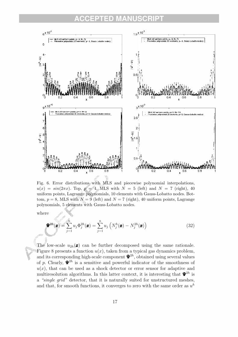
Figures 6 and 7 present the errors in the interpolation of u = sin(2πx) in thedomain [0, +1]. The function value is interpolated at 800 points for plotting,using 40 point values for MLS. Several values of p and N will be discussed, andthe smoothing length is defined as before. The function is also interpolatedusing piecewise polynomials, with a number of elements such that the gridresolution h/p is the same as that of the MLS point distribution, and with thenodes placed at the Gauss-Lobatto points. Figure 6 plots the error distributionfor p = 4 and p = 8. The MLS points are evenly spaced. When the minimumnumber of neighbours, p + 1, is used (top left and bottom left, respectively),the accuracy of MLS for interior nodes is significantly higher than that of thepiecewise polynomial interpolation. Furthermore, note that the difference in-creases with the approximation order. Note that in figure 7 the solutions werecomputed using random points (MLS), and the optimal Gauss-Lobatto nodedistribution (piecewise polynomial), respectively. For redundant point clouds,N > p + 1, (figure 6, top right and bottom right), the piecewise polynomialinterpolation is more accurate, although the differences for interior points aresmall. We must point out that generating good non-uniform nodal distribu-tions for high order piecewise polynomial interpolants is straightforward in 1D(the Gauss-Lobatto points are optimal), but the multidimensional case is farfrom being so, particularly in the case of methods that use cell subdivisionson triangles.

One of the main shortcomings of MLS approximants is also apparent from fig-ures 6–7. For p = 8, the interpolation errors near the boundaries of the globaldomain are about an order of magnitude higher than those inside the domain.This is associated to the one-sided MLS approximation, and is more and morepronounced as p is increased. We must point out that suboptimal node dis-tributions for piecewise polynomial interpolations would have the same effect,

14

ACCEPTED MANUSCRIPT

but in this case on all cells, not just near the domain boundaries as MLS. Webelieve that this effect is less important for most practical values of p (maybeup to p = 5), and that it can be alleviated by the use of ghost points andspecial boundary kernels.

Another potential weakness of MLS is the conditioning of the moment matrix,either due to the cloud structure (highly anisotropic grids), or to very highvalues of p. In multidimensions the definition of the stencil is probably a morestringent limitation to stay in p’s up to 4 or 5 in 2D/3D, which, on the otherhand, is enough for most practical applications. The use of anisotropic kernelsthat adapt to the point distribution helps providing robustness in generalgrids, but the question is far from being resolved.

Fig. 4. MLS shape functions for p = 5, N = 9 (bottom left), and p = 10, N = 15(bottom right). Lagrange basis for p = 5 (top left) and p = 10 (top right).

3.4 Multiple scale analysis and shock detection.

One of the most interesting features of the MLS approximation stems from itsnatural connection to wavelets and their intrinsic property of multiresolutionanalysis (see [19] and references therein). Consider a function u(xxxxxxxxxxxxxx), and define

15

ACCEPTED MANUSCRIPT

Fig. 5. MLS shape functions for p = 10: N = 15 uniform points (top left), N = 19uniform points (top right), N = 15 Gauss-Lobatto points (bottom left) and N = 15random points (bottom right).

two sets of MLS shape functions, NNNNNNNNNNNNNNh(xxxxxxxxxxxxxx) and NNNNNNNNNNNNNN2h(xxxxxxxxxxxxxx), computed using twodifferent values of the smoothing lenght, h and 2h, which respectively defineh-scale and 2h-scale approximations of the form

uh(xxxxxxxxxxxxxx) =n∑

j=1

ujNhj (xxxxxxxxxxxxxx) u2h(xxxxxxxxxxxxxx) =

n∑

j=1

ujN2hj (xxxxxxxxxxxxxx) (29)

A set of wavelet functions is obtained as

ΦΦΦΦΦΦΦΦΦΦΦΦΦΦ2h(xxxxxxxxxxxxxx) = NNNNNNNNNNNNNNh(xxxxxxxxxxxxxx)−NNNNNNNNNNNNNN2h(xxxxxxxxxxxxxx) (30)

which allow the h-scale solution to be expressed as the sum of its low-scaleand high-scale complementary parts, as

uh(xxxxxxxxxxxxxx) = u2h(xxxxxxxxxxxxxx) + ΨΨΨΨΨΨΨΨΨΨΨΨΨΨ2h(xxxxxxxxxxxxxx) (31)

16

ACCEPTED MANUSCRIPT

Fig. 6. Error distributions with MLS and piecewise polynomial interpolations,u(x) = sin(2πx). Top, p = 4, MLS with N = 5 (left) and N = 7 (right), 40uniform points, Lagrange polynomials, 10 elements with Gauss-Lobatto nodes. Bot-tom, p = 8, MLS with N = 9 (left) and N = 7 (right), 40 uniform points, Lagrangepolynomials, 5 elements with Gauss-Lobatto nodes.

where

ΨΨΨΨΨΨΨΨΨΨΨΨΨΨ2h(xxxxxxxxxxxxxx) =n∑

j=1

ujΦ2hj (xxxxxxxxxxxxxx) =

n∑

j=1

uj

(Nh

j (xxxxxxxxxxxxxx)−N2hj (xxxxxxxxxxxxxx)

)(32)

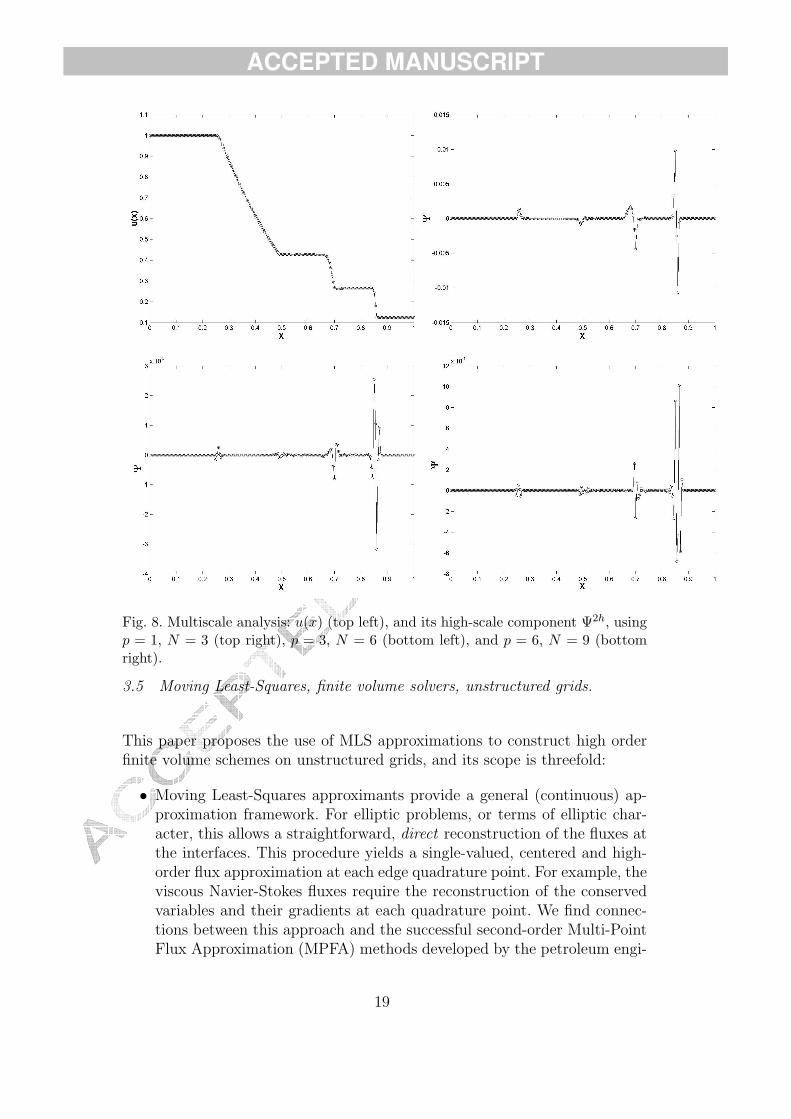
The low-scale u2h(xxxxxxxxxxxxxx) can be further decomposed using the same rationale.Figure 8 presents a function u(x), taken from a typical gas dynamics problem,and its corresponding high-scale component ΨΨΨΨΨΨΨΨΨΨΨΨΨΨ2h, obtained using several valuesof p. Clearly, ΨΨΨΨΨΨΨΨΨΨΨΨΨΨ2h is a sensitive and powerful indicator of the smoothness ofu(x), that can be used as a shock detector or error sensor for adaptive andmultiresolution algorithms. In this latter context, it is interesting that ΨΨΨΨΨΨΨΨΨΨΨΨΨΨ2h isa “single grid” detector, that it is naturally suited for unstructured meshes,and that, for smooth functions, it converges to zero with the same order as uh

17

ACCEPTED MANUSCRIPT

Fig. 7. Error distributions with MLS and piecewise polynomial interpolations,u(x) = sin(2πx). Left, p = 4, MLS with N = 5, 40 random points, Lagrange poly-nomials, 10 elements with Gauss-Lobatto nodes. Right, p = 8, MLS with N = 9, 40random points, Lagrange polynomials, 5 elements with Gauss-Lobatto nodes.

does, p + 1 (it is identically zero for polynomials of degree equal or less thanp).

We believe that this multiresolution smoothness indicator, and its straightfor-ward incorporation into a code that already uses MLS approximations (oneonly needs to compute another set of shape functions, but with 2h instead ofh), is a very attractive feature of the proposed methodology. Even though wellbehaved limiters for second order schemes have been developed, the questionfor higher order reconstructions is far from being clear. Therefore, selectiveshock-capturing is a critical issue for higher-order schemes. If the limiters areactive over the whole domain, their effect on higher order derivatives resultsinto a partial (or, quite frequently, complete) loss of the higher order accu-racy of the reconstruction in smooth regions of the flow, virtually taking themethod back to second order.

As it is shown in one of the simulations in section 6, the limiters can beswitched off in those areas where ΨΨΨΨΨΨΨΨΨΨΨΨΨΨ2h is lower than a certain threshold, there-fore retaining the whole accuracy of the scheme in smooth regions. Note thatthe concept of “smooth region” itself is strongly related to the approximationbeing used, and hence the convenience of an indicator that is of the sameorder and nature as the approximants. In some sense, this procedure can beregarded as an unstructured grid generalization of the wavelet-based selectivefiltering proposed by Sjogreen and Yee for finite differences [20].

18

ACCEPTED MANUSCRIPT

Fig. 8. Multiscale analysis: u(x) (top left), and its high-scale component Ψ2h, usingp = 1, N = 3 (top right), p = 3, N = 6 (bottom left), and p = 6, N = 9 (bottomright).

3.5 Moving Least-Squares, finite volume solvers, unstructured grids.

This paper proposes the use of MLS approximations to construct high orderfinite volume schemes on unstructured grids, and its scope is threefold:

• Moving Least-Squares approximants provide a general (continuous) ap-proximation framework. For elliptic problems, or terms of elliptic char-acter, this allows a straightforward, direct reconstruction of the fluxes atthe interfaces. This procedure yields a single-valued, centered and high-order flux approximation at each edge quadrature point. For example, theviscous Navier-Stokes fluxes require the reconstruction of the conservedvariables and their gradients at each quadrature point. We find connec-tions between this approach and the successful second-order Multi-PointFlux Approximation (MPFA) methods developed by the petroleum engi-

19

ACCEPTED MANUSCRIPT

neering community (see [18] for an introduction).• For hyperbolic problems, or terms of hyperbolic character, the general-

ized Godunov method [10,11,16] is adopted. We use “broken” piecewisepolynomial reconstructions based on the MLS general approximation andTaylor series expansions. The succesive derivatives of the flow variablesat the cell centroids are computed using MLS approximations. There-fore, rather than creating new degrees of freedom inside each cell, we useinformation from neighbouring cells, in a centered (moving) fashion.

• The MLS-based multiresolution indicator provides a reliable shock-detectiontool for the selective limiting of higher-order discretizations.

4 Practical Implementation Aspects

4.1 Overview.

The following sections elaborate on the practical implementation of the pro-posed methodology. Conceptually, two aspects of the process should be dis-tinguised:

• How the MLS shape functions and their derivatives are computed; inparticular, the choice of the cloud of neighbours for each evaluation point(centroids or edge quadrature points). We call these clouds the stencilof the MLS approximation. This choice ultimately determines the fullstencil of the finite volume method.

• How the MLS shape functions and their derivatives are used to 1) con-struct high order reconstructions for a Godunov-type scheme for hyper-bolic problems and to 2) directly reconstruct the “viscous” fluxes at theedges, thus obtaining a multipoint-like high order scheme for elliptic prob-lems.

Sections 4.2 and 4.3 present the MLS stencils used in this study for the cubicbasis (p = 3).

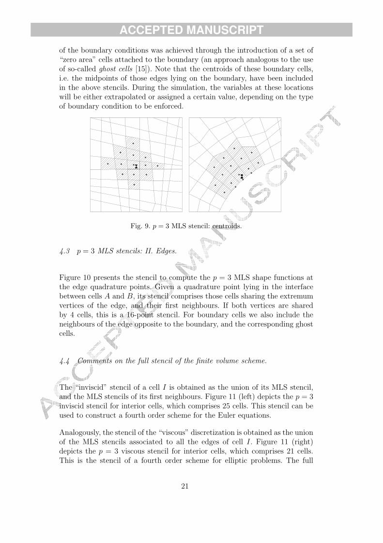
4.2 p = 3 MLS stencils: I. Centroids.

Figure 9 presents the stencil used to compute the p = 3 MLS shape funtionsat the cell centroids. For and interior cell I, the stencil comprises its first andsecond neighbours (by neighbours we mean cells that share an edge). This givesa 13-point stencil. For boundary cells the stencil comprises those cells thatshare a vertex with the cell and their first neighbours. A stronger enforcement

20

ACCEPTED MANUSCRIPT

of the boundary conditions was achieved through the introduction of a set of“zero area” cells attached to the boundary (an approach analogous to the useof so-called ghost cells [15]). Note that the centroids of these boundary cells,i.e. the midpoints of those edges lying on the boundary, have been includedin the above stencils. During the simulation, the variables at these locationswill be either extrapolated or assigned a certain value, depending on the typeof boundary condition to be enforced.

Fig. 9. p = 3 MLS stencil: centroids.

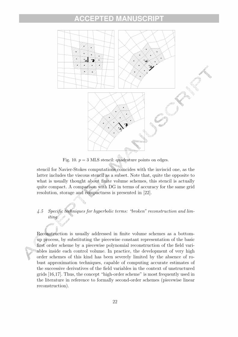
4.3 p = 3 MLS stencils: II. Edges.

Figure 10 presents the stencil to compute the p = 3 MLS shape functions atthe edge quadrature points. Given a quadrature point lying in the interfacebetween cells A and B, its stencil comprises those cells sharing the extremumvertices of the edge, and their first neighbours. If both vertices are sharedby 4 cells, this is a 16-point stencil. For boundary cells we also include theneighbours of the edge opposite to the boundary, and the corresponding ghostcells.

4.4 Comments on the full stencil of the finite volume scheme.

The “inviscid” stencil of a cell I is obtained as the union of its MLS stencil,and the MLS stencils of its first neighbours. Figure 11 (left) depicts the p = 3inviscid stencil for interior cells, which comprises 25 cells. This stencil can beused to construct a fourth order scheme for the Euler equations.

Analogously, the stencil of the “viscous” discretization is obtained as the unionof the MLS stencils associated to all the edges of cell I. Figure 11 (right)depicts the p = 3 viscous stencil for interior cells, which comprises 21 cells.This is the stencil of a fourth order scheme for elliptic problems. The full

21

ACCEPTED MANUSCRIPT

Fig. 10. p = 3 MLS stencil: quadrature points on edges.

stencil for Navier-Stokes computations coincides with the inviscid one, as thelatter includes the viscous stencil as a subset. Note that, quite the opposite towhat is usually thought about finite volume schemes, this stencil is actuallyquite compact. A comparison with DG in terms of accuracy for the same gridresolution, storage and compactness is presented in [22].

4.5 Specific techniques for hyperbolic terms: “broken” reconstruction and lim-iting.

Reconstruction is usually addressed in finite volume schemes as a bottom-up process, by substituting the piecewise constant representation of the basicfirst order scheme by a piecewise polynomial reconstruction of the field vari-ables inside each control volume. In practice, the development of very highorder schemes of this kind has been severely limited by the absence of ro-bust approximation techniques, capable of computing accurate estimates ofthe successive derivatives of the field variables in the context of unstructuredgrids [16,17]. Thus, the concept “high-order scheme” is most frequently used inthe literature in reference to formally second-order schemes (piecewise linearreconstruction).

22

ACCEPTED MANUSCRIPT

Fig. 11. Fourth order MLS-FV stencil: Euler and Navier-Stokes (left) and ellipticproblems (right).

In contrast, our approach is top-down, as we define a general continuous ap-proximation framework provided by the Moving Least-Squares approximants,and then compute local discontinuous approximations, which are broken high-order approximations to the underlying continuous solution, to be used in thecontext of a Godunov-type scheme. In this study, reconstructions of up tofourth order (cubic) have been tested, although schemes of up to sixth orderare expected to be practical in the near future.

The linear component-wise reconstruction of the variables inside cell I reads

U(xxxxxxxxxxxxxx) = UI +∇∇∇∇∇∇∇∇∇∇∇∇∇∇UI · (xxxxxxxxxxxxxx− xxxxxxxxxxxxxxI) (33)

where UI stands for the centroid value, xxxxxxxxxxxxxxI denotes spatial coordinates of thecentroid of the cell and ∇∇∇∇∇∇∇∇∇∇∇∇∇∇UI is a cell-centered gradient. This gradient is as-sumed to be constant on each cell and, therefore, the reconstructed variablesare discontinuous across interfaces.

Analogously, the quadratic reconstruction reads

U(xxxxxxxxxxxxxx) = UI +∇∇∇∇∇∇∇∇∇∇∇∇∇∇UI · (xxxxxxxxxxxxxx− xxxxxxxxxxxxxxI) +1

2(xxxxxxxxxxxxxx− xxxxxxxxxxxxxxI)

THHHHHHHHHHHHHHI(xxxxxxxxxxxxxx− xxxxxxxxxxxxxxI) (34)

where HHHHHHHHHHHHHHI is the centroid hessian matrix. Finally, the cubic reconstruction canbe written as

U(xxxxxxxxxxxxxx) = UI +∇∇∇∇∇∇∇∇∇∇∇∇∇∇UI · (xxxxxxxxxxxxxx− xxxxxxxxxxxxxxI) +1

2(xxxxxxxxxxxxxx− xxxxxxxxxxxxxxI)

THHHHHHHHHHHHHHI(xxxxxxxxxxxxxx− xxxxxxxxxxxxxxI)

23

ACCEPTED MANUSCRIPT

+1

6∆∆∆∆∆∆∆∆∆∆∆∆∆∆2xxxxxxxxxxxxxxT

I TTTTTTTTTTTTTT I(xxxxxxxxxxxxxx− xxxxxxxxxxxxxxI) (35)

where

∆∆∆∆∆∆∆∆∆∆∆∆∆∆2xxxxxxxxxxxxxxTI =

((x− xI)

2 (y − yI)2), TTTTTTTTTTTTTT I =

∂3UI

∂x33

∂3UI

∂x2∂y

3∂3UI

∂x∂y2

∂3UI

∂y3

(36)

For unsteady problems, additional terms must be introduced in (34) and (35)to enforce conservation of the mean, i.e.

1

AI

∫

xxxxxxxxxxxxxx∈ΩI

U (xxxxxxxxxxxxxx) dΩ = UI (37)

The derivatives of the field variables are directly computed at centroids usingMLS. Thus, the approximate gradients read

∇∇∇∇∇∇∇∇∇∇∇∇∇∇UI =

nxxxxxxxxxxxxxxI∑

j=1

Uj∇∇∇∇∇∇∇∇∇∇∇∇∇∇Nj(xxxxxxxxxxxxxxI) (38)

where the Uj’s stand for variables at the nxxxxxxxxxxxxxxI“neighbour” (in the sense of the

MLS stencil) centroids. The second order derivatives read

∂2UI

∂x2=

nxxxxxxxxxxxxxxI∑

j=1

Uj∂2Nj(xxxxxxxxxxxxxxI)

∂x2

∂2UI

∂x∂y=

nxxxxxxxxxxxxxxI∑

j=1

Uj∂2Nj(xxxxxxxxxxxxxxI)

∂x∂y

∂2UI

∂y2=

nxxxxxxxxxxxxxxI∑

j=1

Uj∂2Nj(xxxxxxxxxxxxxxI)

∂y2(39)

Finally, the third order derivatives are written as

∂3UI

∂x3=

nxxxxxxxxxxxxxxI∑

j=1

Uj∂3Nj(xxxxxxxxxxxxxxI)

∂x3,

∂3UI

∂x2∂y=

nxxxxxxxxxxxxxxI∑

j=1

Uj∂3Nj(xxxxxxxxxxxxxxI)

∂x2∂y

∂3UI

∂x∂y2=

nxxxxxxxxxxxxxxI∑

j=1

Uj∂3Nj(xxxxxxxxxxxxxxI)

∂x∂y2,

∂3UI

∂y3=

nxxxxxxxxxxxxxxI∑

j=1

Uj∂3Nj(xxxxxxxxxxxxxxI)

∂y3(40)

In this study, the first order derivatives were computed as full MLS derivatives,whereas the second and third order derivatives are approximated by the diffuseones.

24

ACCEPTED MANUSCRIPT

In the presence of shocks, some limiting procedure is applied to the abovederivatives. The choice of adequate multidimensional limiters is critical inorder to achieve accurate and non-oscillatory shock-capturing algorithms.

4.5.1 Limiters: I.Monotonicity enforcement.

Barth and Jespersen [12] have proposed an extension of Van Leer’s scheme [25]which is suitable for unstructured grids. The basic idea is to enforce “mono-tonicity” in the reconstructed solution. In this context, monotonicity impliesthat no new extrema are created by the reconstruction process [12]. The en-forcement is local, in the sense that only certain neighbour cells are consideredfor the “no new extrema” criterion.

Recall the piecewise linear reconstruction U(xxxxxxxxxxxxxx)I of a variable U inside a certaincell I

U(xxxxxxxxxxxxxx)I = UI +∇∇∇∇∇∇∇∇∇∇∇∇∇∇UI · (xxxxxxxxxxxxxx− xxxxxxxxxxxxxxI) (41)

and consider a limited version of this reconstruction, as

U(xxxxxxxxxxxxxx)I = UI + ΦI∇∇∇∇∇∇∇∇∇∇∇∇∇∇UI · (xxxxxxxxxxxxxx− xxxxxxxxxxxxxxI) (42)

where ΦI is a slope limiter (0 ≤ ΦI ≤ 1) such that the reconstruction (42)satisfies

Umin ≤ U(xxxxxxxxxxxxxx)I ≤ Umax (43)

being

Umin = minj∈AI

(Uj), Umax = maxj∈AI

(Uj) (44)

where AI is the set of “neighbour” cells. In practice, the restriction (43) isonly enforced at the quadrature points on the edges of cell I; thus, for eachquadrature point q, its associated slope limiter Φq

I is computed in terms of theunlimited extrapolated value U q

I , as

ΦqI =

min

(1,

Umax − UI

U qI − UI

)U q

I − UI > 0

min

(1,

Umin − UI

U qI − UI

)U q

I − UI < 0

1 U qI − UI = 0

(45)

25

ACCEPTED MANUSCRIPT

and, finally,

ΦI = minq

(ΦqI) (46)

In the case of the quadratic reconstruction, (34), a similar limiting strategy isadopted

U(xxxxxxxxxxxxxx) = UI + ΦI

(∇∇∇∇∇∇∇∇∇∇∇∇∇∇UI · (xxxxxxxxxxxxxx− xxxxxxxxxxxxxxI) +

1

2(xxxxxxxxxxxxxx− xxxxxxxxxxxxxxI)

THHHHHHHHHHHHHHI(xxxxxxxxxxxxxx− xxxxxxxxxxxxxxI))

(47)

where the limiter ΦI is obtained following the same procedure exposed abovefor the linear case. An analogous expression can be used for the cubic recon-struction.

In this study the neighbourhood to determine the extrema Umin and Umax

comprises the reconstruction cell I and its first order neighbours (figure 12–A). In the following, the above limiter will be referred to as “BJ limiter”.

Fig. 12. Neighbourhoods for the limiting of the reconstruction inside cell I.

4.5.2 Limiters: II.Averaged derivatives.

This section presents a general strategy to obtain limited gradients and hessianmatrices. Thus, the limited gradient associated to a certain cell I, ∇∇∇∇∇∇∇∇∇∇∇∇∇∇UI is

26

ACCEPTED MANUSCRIPT

obtained as a weighted average of a series of representative gradients, as

∇∇∇∇∇∇∇∇∇∇∇∇∇∇UI =N∑

k=1

ωk∇∇∇∇∇∇∇∇∇∇∇∇∇∇Uk (48)

where ∇∇∇∇∇∇∇∇∇∇∇∇∇∇Uk, k = 1, . . . , N is a set of unlimited gradients, used as a basisto construct the limited one. In an approach similar to that exposed in [15],the weights ωk, k = 1, . . . , N are given by

ωk (g1, g2, · · · , gN) =

N∏i6=k

gi + εN−1

N∑j=1

(N∏

i 6=jgi

)+ NεN−1

k = 1, . . . , N (49)

where gi, i = 1, . . . , N are functions of the unlimited gradients (in thisstudy, gi = ‖∇∇∇∇∇∇∇∇∇∇∇∇∇∇Ui‖2) and ε is a small number, introduced to avoid divisionby zero. The hessian matrices will also be limited following these ideas but, inthis case, the functions gi read

gi =

(∂2Ui

∂x2

)2

+ 2

(∂2Ui

∂x∂y

)2

+

(∂2Ui

∂y2

)2

i = 1, . . . , N (50)

Some existing limiters could be considered to be included in this family. VanRosendale [26] has proposed an extension to three gradients of Van Albada’slimiter [27]. This limiter was used on unstructured triangular grids and itsgeneral structure is that of (48) with N = 3. The representative gradients areevaluated at the three vertices of the cell. Jawahar and Kamath [15] proposeda limiter with N = 3, with averaged gradients computed from the unlimitedgradients evaluated at the centroids of the adyacent cells on triangular meshes.Furthermore, the denominators in (49) are slightly different in this case.

For quadrilateral cells we propose a limiter based on (48)–(49) with N = 5;i.e. the limited derivatives are obtained as a weighted average of five unlimitedderivatives. Figure 12 presents four suitable configurations to determine suchrepresentative derivatives . In this study only the configuration given by 12–Awill be considered. In the following, the above limiter will be referred to as“PC5 limiter”.

4.6 Numerical convective fluxes.

The numerical inviscid fluxes in (13) are obtained using Roe’s flux differencesplitting [28]. For this purpose, left (UUUUUUUUUUUUUU+) and right (UUUUUUUUUUUUUU−) states are defined on

27

ACCEPTED MANUSCRIPT

each face. The numerical flux is then computed as

(FFFFFFFFFFFFFF x, FFFFFFFFFFFFFF y) · nnnnnnnnnnnnnn =1

2

[(FFFFFFFFFFFFFF x

(UUUUUUUUUUUUUU+

), FFFFFFFFFFFFFF y

(UUUUUUUUUUUUUU+

))+

(FFFFFFFFFFFFFF x

(UUUUUUUUUUUUUU−)

, FFFFFFFFFFFFFF y

(UUUUUUUUUUUUUU−))]

· nnnnnnnnnnnnnn−1

2

3∑

k=1

αk|λk|rrrrrrrrrrrrrrk (51)

where λk, k = 1, 4 and rrrrrrrrrrrrrrk, k = 1, 4 are, respectively, the eigenvalues and

eigenvectors of the approximate jacobian JJJJJJJJJJJJJJ(UUUUUUUUUUUUUU+,UUUUUUUUUUUUUU−)

λ1 = vvvvvvvvvvvvvv · nnnnnnnnnnnnnn− c, λ2 = λ3 = vvvvvvvvvvvvvv · nnnnnnnnnnnnnn, λ4 = vvvvvvvvvvvvvv · nnnnnnnnnnnnnn + c (52)

(rrrrrrrrrrrrrr1 rrrrrrrrrrrrrr2 rrrrrrrrrrrrrr3 rrrrrrrrrrrrrr4) =

1 0 1 0u− cnx −cny u u + cnx

v − cny cnx v v + cny

H − c vvvvvvvvvvvvvv · nnnnnnnnnnnnnn c(vnx − uny)12(u2 + v2) H + c vvvvvvvvvvvvvv · nnnnnnnnnnnnnn

(53)

and the corresponding wave strengths αk, k = 1, 4

α1 =1

2c2[∆ (p)− ρc (∆ (u) nx + ∆ (v) ny)]

α2 =ρ

c[∆ (v) nx −∆ (u) ny]

α3 = − 1

c2

[∆ (p)− c2∆ (ρ)

]

α4 =1

2c2[∆ (p) + ρc (∆ (u) nx + ∆ (v) ny)] (54)

where ∆ (·) = (·)−− (·)+, nnnnnnnnnnnnnn = (nx, ny) is the outward pointing unit normal to

the interface, and the Roe-average values vvvvvvvvvvvvvv = (u, v) and H (computed usingUUUUUUUUUUUUUU+ and UUUUUUUUUUUUUU−) are defined as

u =u+√

ρ+ + u−√

ρ−√ρ+ +

√ρ−

v =v+√

ρ+ + v−√

ρ−√ρ+ +

√ρ−

H =H+

√ρ+ + H−√ρ−√ρ+ +

√ρ−

(55)

On the other hand, the average values ρ and c are computed as

ρ =√

ρ+ρ− c2 = (γ − 1)[H − 1

2

(u2 + v2

)](56)

4.7 Viscous fluxes.

As mentioned before, one of the major advantages of the proposed method isthat we use the MLS approximants as a global (centered) reconstruction pro-

28

ACCEPTED MANUSCRIPT

cedure to evaluate the viscous fluxes at the quadrature points on the edges.This procedure provides a single high-order flux and, therefore, it is not nec-essary to create new degrees of freedom to compute the derivatives of thevariables at the cell edges.

Recall that the evaluation of the viscous stresses and heat fluxes requiresinterpolating the velocity vector vvvvvvvvvvvvvv = (u, v), temperature T , and their corre-sponding gradients, ∇∇∇∇∇∇∇∇∇∇∇∇∇∇vvvvvvvvvvvvvv and ∇∇∇∇∇∇∇∇∇∇∇∇∇∇T , at each quadrature point xxxxxxxxxxxxxxiq. Using MLSapproximation, these entities are readily computed as

vvvvvvvvvvvvvviq =niq∑

j=1

vvvvvvvvvvvvvvjNj(xxxxxxxxxxxxxxiq), Tiq =niq∑

j=1

TjNj(xxxxxxxxxxxxxxiq) (57)

and

∇∇∇∇∇∇∇∇∇∇∇∇∇∇vvvvvvvvvvvvvviq =niq∑

j=1

vvvvvvvvvvvvvvj ⊗∇∇∇∇∇∇∇∇∇∇∇∇∇∇Nj(xxxxxxxxxxxxxxiq), ∇∇∇∇∇∇∇∇∇∇∇∇∇∇Tiq =niq∑

j=1

Tj∇∇∇∇∇∇∇∇∇∇∇∇∇∇Nj(xxxxxxxxxxxxxxiq) (58)

where niq is the number of neighbour centroids (in the sense of the MLSstencil). Once the above information has been interpolated, the diffusive fluxescan be computed, according to (3).

4.8 Flux integration.

One quadrature point (the midpoint) was used in the case of linear recon-struction, whereas two and three Gauss points were respectively used in thecase of quadratic and cubic reconstructions.

4.9 Time integration.

We use the third order TVD-Runge-Kutta algorithm proposed by Shu andOsher [29]. Given the field variables Un at the previous time step n, the al-gorithm proceeds in three stages to obtain the updated field variables Un+1,as

U1 = Un + ∆tL(Un)

U2 =3

4Un +

1

4U1 +

1

4∆tL(U1)

Un+1 =1

3Un +

2

3U2 +

2

3∆tL(U2) (59)

29

ACCEPTED MANUSCRIPT

where the operator L(·), which represents the time derivative given by (13),reads

L(UUUUUUUUUUUUUU) =1

A

nedge∑

iedge=1

ngau∑

igau=1

[(FFFFFFFFFFFFFFV −FFFFFFFFFFFFFF

)· nnnnnnnnnnnnnn

]igau

Wigau (60)

5 Accuracy tests

This section presents some convergence results of the proposed finite volumemethod with Moving Least-Squares approximations. The tests are intended toassess the performance of the methodology with respect to two distinct areasof its scope: high-order variable reconstruction for Godunov-type schemes, andhigh-order, multi-point viscous flux evaluation.

5.1 Hyperbolic problems: Ringleb flow.

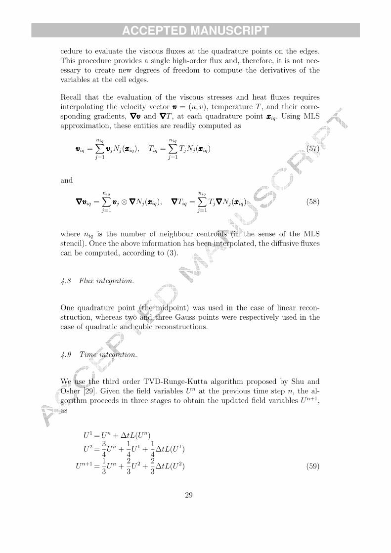
Ringleb flow is an exact solution of the Euler equations, obtained by means ofthe hodograph method [30]. The problem is solved on the square [−1.15,−0.75]×[+0.15, +0.55], imposing the exact value of the conserved variables on theboundary. Linear, quadratic and cubic reconstructions are developed by meansof MLS derivatives, as exposed above. A refinement study was carried out us-ing a sequence of four nested grids, the coarsest of which is showed in figure13 (top), along with the convergence curves, which are broken down in table1.

All linear, quadratic and cubic reconstructions exhibit the correct second,third and fourth orders of convergence, respectively, as expected. One, two,and three Gauss quadrature points per edge have been employed for the sec-ond, third, and fourth order schemes, respectively. In addition, figure 13 (bot-tom right) presents a comparison of the different reconstructions with respectto accuracy versus workload. The cpu times are expressed in terms of timeunits per time step of the Runge-Kutta integrator, and normalized with re-spect to the cpu time associated to a time step of the first-order scheme (noreconstruction) on the 10× 10 grid, which is taken as the reference workload,Work = 1. The benefits and efficiency of the higher order reconstructions arequite apparent. Comparing the second and fourth order reconstructions, forexample, we see that, for the same grid, the accuracy of the latter is aboutthree orders of magnitude higher than that of the former, with a cpu increaseof a factor of four. Moreover, most of the additional cpu time associated to thefourth order scheme is due to the use of three quadrature points per edge, andtherefore more flux evaluations, and not to the higher order reconstruction

30

ACCEPTED MANUSCRIPT

itself.

Linear rec. Quadratic rec. Cubic rec.

Grid Work L2 error Slope Work L2 error Slope Work L2 error Slope

10× 10 1.3 5.04 10−5 2.1 4.71 10−6 4 1.39 10−7

20× 20 3.5 1.28 10−5 1.98 6.8 2.23 10−7 4.40 12.6 1.06 10−8 3.71

40× 40 11 3.14 10−6 2.03 23 2.34 10−8 3.25 42.5 6.60 10−9 4.01

80× 80 35 7.81 10−7 2.01 80.5 2.80 10−9 3.06 152 4.07 10−10 4.02Table 1Fourth order results

Fig. 13. Coarse grid level and convergence results for Ringleb flow.

31

ACCEPTED MANUSCRIPT

5.2 Viscous discretization. A first “worked” example: 1D Poisson.

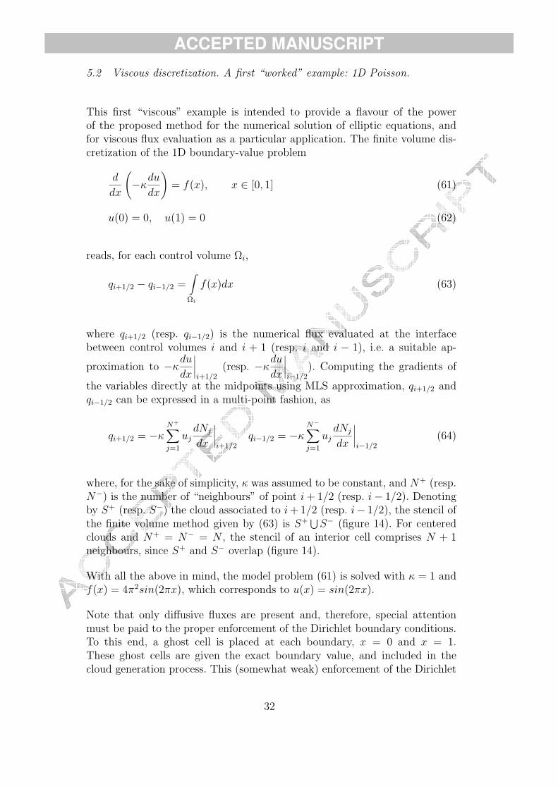
This first “viscous” example is intended to provide a flavour of the powerof the proposed method for the numerical solution of elliptic equations, andfor viscous flux evaluation as a particular application. The finite volume dis-cretization of the 1D boundary-value problem

d

dx

(−κ

du

dx

)= f(x), x ∈ [0, 1] (61)

u(0) = 0, u(1) = 0 (62)

reads, for each control volume Ωi,

qi+1/2 − qi−1/2 =∫

Ωi

f(x)dx (63)

where qi+1/2 (resp. qi−1/2) is the numerical flux evaluated at the interfacebetween control volumes i and i + 1 (resp. i and i − 1), i.e. a suitable ap-

proximation to −κdu

dx

∣∣∣∣i+1/2

(resp. −κdu

dx

∣∣∣∣i−1/2

). Computing the gradients of

the variables directly at the midpoints using MLS approximation, qi+1/2 andqi−1/2 can be expressed in a multi-point fashion, as

qi+1/2 = −κN+∑

j=1

ujdNj

dx

∣∣∣∣i+1/2

qi−1/2 = −κN−∑

j=1

ujdNj

dx

∣∣∣∣i−1/2

(64)

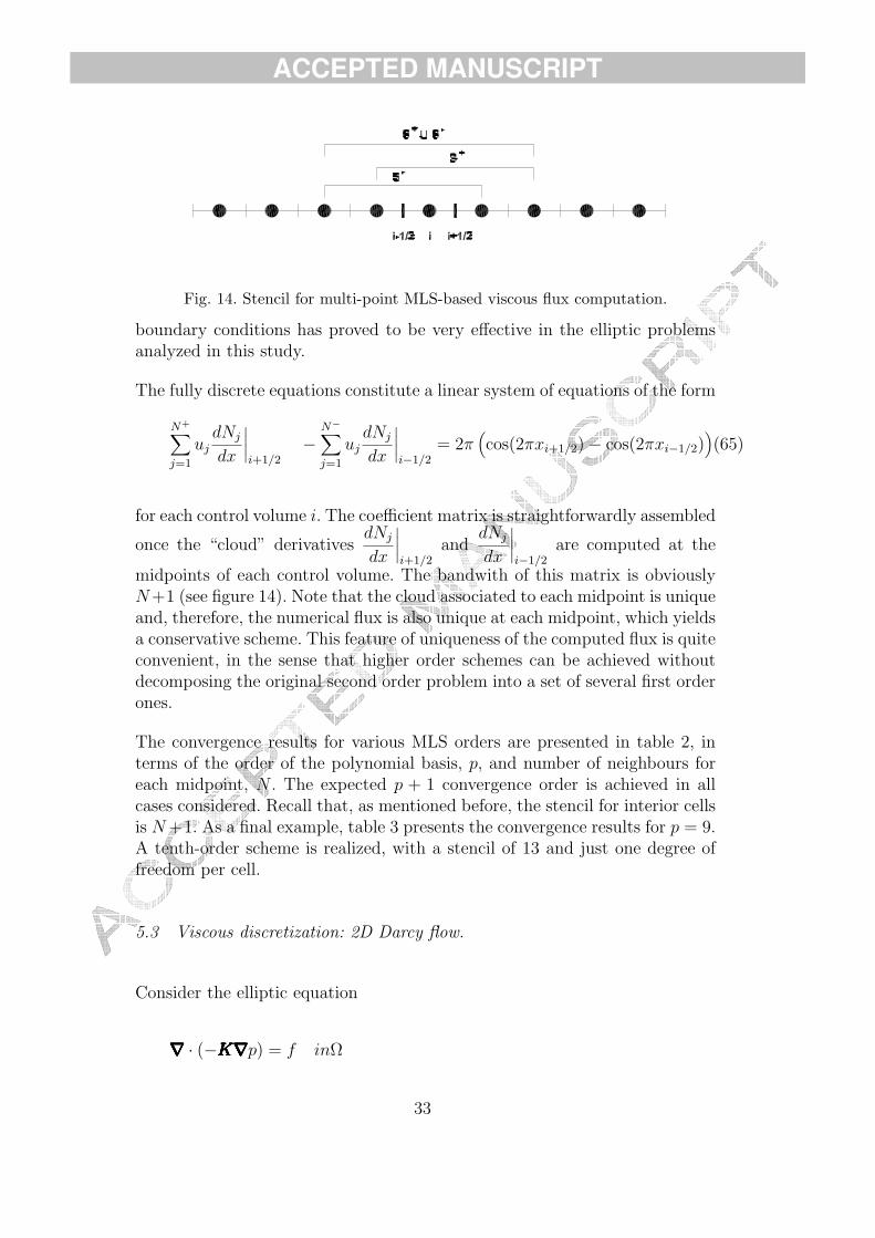
where, for the sake of simplicity, κ was assumed to be constant, and N+ (resp.N−) is the number of “neighbours” of point i + 1/2 (resp. i− 1/2). Denotingby S+ (resp. S−) the cloud associated to i + 1/2 (resp. i− 1/2), the stencil ofthe finite volume method given by (63) is S+ ⋃

S− (figure 14). For centeredclouds and N+ = N− = N , the stencil of an interior cell comprises N + 1neighbours, since S+ and S− overlap (figure 14).

With all the above in mind, the model problem (61) is solved with κ = 1 andf(x) = 4π2sin(2πx), which corresponds to u(x) = sin(2πx).

Note that only diffusive fluxes are present and, therefore, special attentionmust be paid to the proper enforcement of the Dirichlet boundary conditions.To this end, a ghost cell is placed at each boundary, x = 0 and x = 1.These ghost cells are given the exact boundary value, and included in thecloud generation process. This (somewhat weak) enforcement of the Dirichlet

32

ACCEPTED MANUSCRIPT

Fig. 14. Stencil for multi-point MLS-based viscous flux computation.

boundary conditions has proved to be very effective in the elliptic problemsanalyzed in this study.

The fully discrete equations constitute a linear system of equations of the form

N+∑

j=1

ujdNj

dx

∣∣∣∣i+1/2

−N−∑

j=1

ujdNj

dx

∣∣∣∣i−1/2

= 2π(cos(2πxi+1/2)− cos(2πxi−1/2)

)(65)

for each control volume i. The coefficient matrix is straightforwardly assembled

once the “cloud” derivativesdNj

dx

∣∣∣∣i+1/2

anddNj

dx

∣∣∣∣i−1/2

are computed at the

midpoints of each control volume. The bandwith of this matrix is obviouslyN+1 (see figure 14). Note that the cloud associated to each midpoint is uniqueand, therefore, the numerical flux is also unique at each midpoint, which yieldsa conservative scheme. This feature of uniqueness of the computed flux is quiteconvenient, in the sense that higher order schemes can be achieved withoutdecomposing the original second order problem into a set of several first orderones.

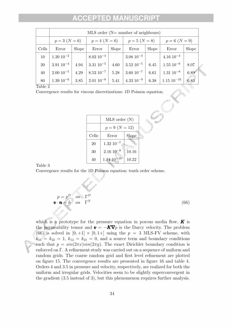
The convergence results for various MLS orders are presented in table 2, interms of the order of the polynomial basis, p, and number of neighbours foreach midpoint, N . The expected p + 1 convergence order is achieved in allcases considered. Recall that, as mentioned before, the stencil for interior cellsis N +1. As a final example, table 3 presents the convergence results for p = 9.A tenth-order scheme is realized, with a stencil of 13 and just one degree offreedom per cell.

5.3 Viscous discretization: 2D Darcy flow.

Consider the elliptic equation

∇∇∇∇∇∇∇∇∇∇∇∇∇∇ · (−KKKKKKKKKKKKKK∇∇∇∇∇∇∇∇∇∇∇∇∇∇p) = f inΩ

33

ACCEPTED MANUSCRIPT

MLS order (N= number of neighbours)

p = 3 (N = 6) p = 4 (N = 6) p = 5 (N = 8) p = 6 (N = 9)

Cells Error Slope Error Slope Error Slope Error Slope

10 1.20 10−2 8.02 10−4 3.08 10−3 4.16 10−4

20 3.91 10−4 4.94 3.31 10−5 4.60 3.52 10−5 6.45 1.55 10−6 8.07

40 2.00 10−5 4.29 8.53 10−7 5.28 3.60 10−7 6.61 1.31 10−8 6.89

80 1.39 10−6 3.85 2.01 10−8 5.41 4.33 10−9 6.38 1.15 10−10 6.83Table 2Convergence results for viscous discretizations: 1D Poisson equation.

MLS order (N)

p = 9 (N = 12)

Cells Error Slope

20 1.32 10−7

30 2.16 10−9 10.16

40 1.14 10−10 10.22Table 3Convergence results for the 1D Poisson equation: tenth order scheme.

p = pD on ΓD

vvvvvvvvvvvvvv · nnnnnnnnnnnnnn = h on ΓN (66)

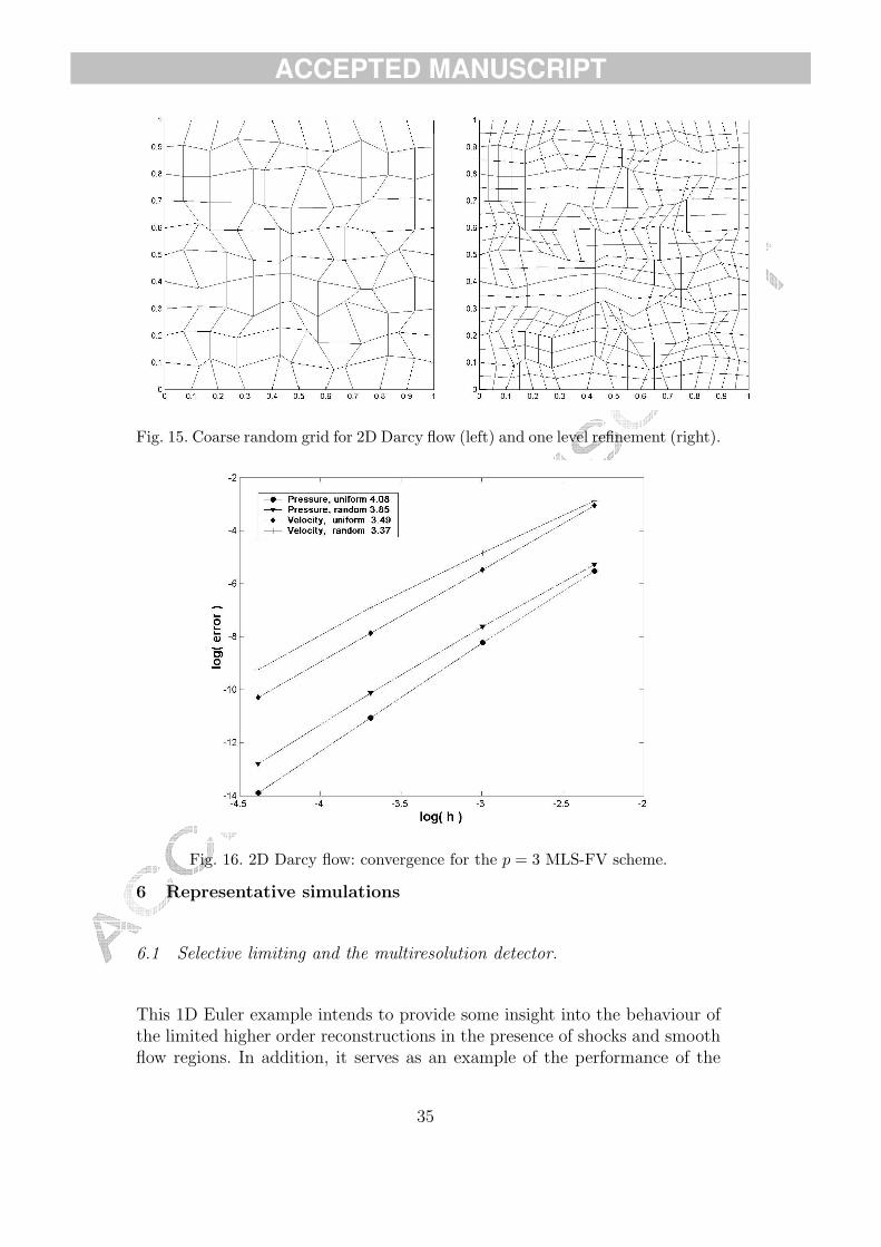
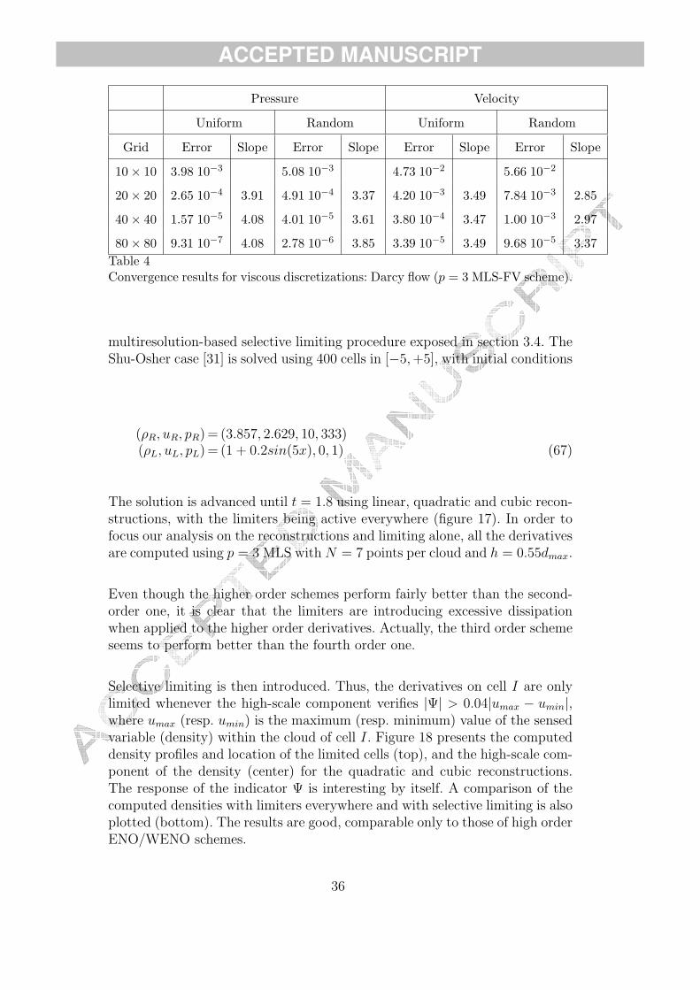
which is a prototype for the pressure equation in porous media flow, KKKKKKKKKKKKKK isthe permeability tensor and vvvvvvvvvvvvvv = −KKKKKKKKKKKKKK∇∇∇∇∇∇∇∇∇∇∇∇∇∇p is the Darcy velocity. The problem(66) is solved in [0, +1] × [0, 1+] using the p = 3 MLS-FV scheme, withk11 = k22 = 1, k12 = k21 = 0, and a source term and boundary conditionssuch that p = sin(2πx)sin(2πy). The exact Dirichlet boundary condition isenforced on Γ. A refinement study was carried out on a sequence of uniform andrandom grids. The coarse random grid and first level refinement are plottedon figure 15. The convergence results are presented in figure 16 and table 4.Orders 4 and 3.5 in pressure and velocity, respectively, are realized for both theuniform and irregular grids. Velocities seem to be slightly superconvergent inthe gradient (3.5 instead of 3), but this phenomenon requires further analysis.

34

ACCEPTED MANUSCRIPT

Fig. 15. Coarse random grid for 2D Darcy flow (left) and one level refinement (right).

Fig. 16. 2D Darcy flow: convergence for the p = 3 MLS-FV scheme.

6 Representative simulations

6.1 Selective limiting and the multiresolution detector.

This 1D Euler example intends to provide some insight into the behaviour ofthe limited higher order reconstructions in the presence of shocks and smoothflow regions. In addition, it serves as an example of the performance of the

35

ACCEPTED MANUSCRIPT

Pressure Velocity

Uniform Random Uniform Random

Grid Error Slope Error Slope Error Slope Error Slope

10× 10 3.98 10−3 5.08 10−3 4.73 10−2 5.66 10−2

20× 20 2.65 10−4 3.91 4.91 10−4 3.37 4.20 10−3 3.49 7.84 10−3 2.85

40× 40 1.57 10−5 4.08 4.01 10−5 3.61 3.80 10−4 3.47 1.00 10−3 2.97

80× 80 9.31 10−7 4.08 2.78 10−6 3.85 3.39 10−5 3.49 9.68 10−5 3.37Table 4Convergence results for viscous discretizations: Darcy flow (p = 3 MLS-FV scheme).

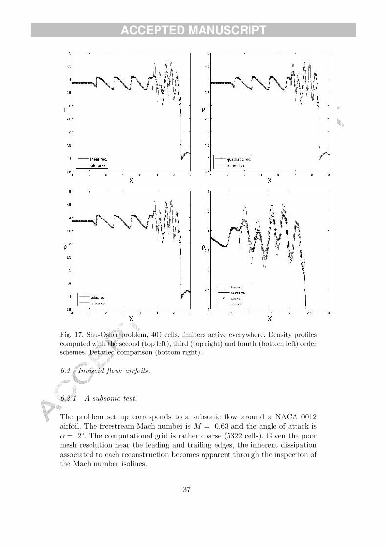
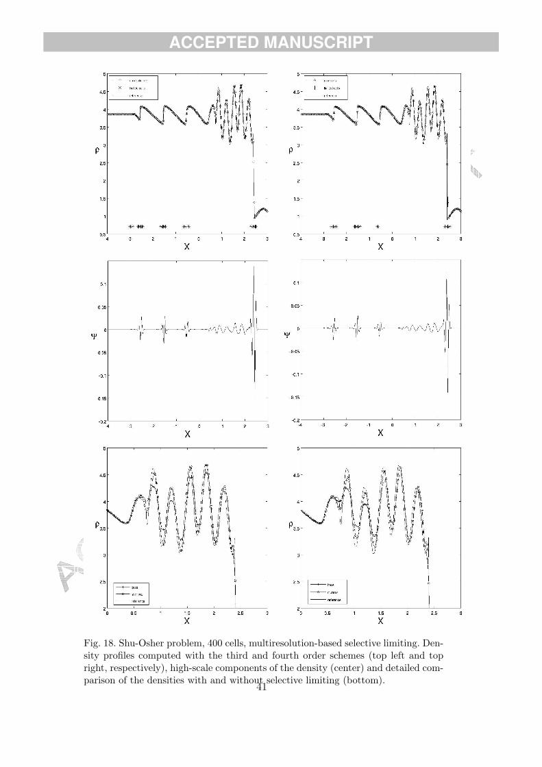
multiresolution-based selective limiting procedure exposed in section 3.4. TheShu-Osher case [31] is solved using 400 cells in [−5, +5], with initial conditions

(ρR, uR, pR) = (3.857, 2.629, 10, 333)(ρL, uL, pL) = (1 + 0.2sin(5x), 0, 1) (67)

The solution is advanced until t = 1.8 using linear, quadratic and cubic recon-structions, with the limiters being active everywhere (figure 17). In order tofocus our analysis on the reconstructions and limiting alone, all the derivativesare computed using p = 3 MLS with N = 7 points per cloud and h = 0.55dmax.

Even though the higher order schemes perform fairly better than the second-order one, it is clear that the limiters are introducing excessive dissipationwhen applied to the higher order derivatives. Actually, the third order schemeseems to perform better than the fourth order one.

Selective limiting is then introduced. Thus, the derivatives on cell I are onlylimited whenever the high-scale component verifies |Ψ| > 0.04|umax − umin|,where umax (resp. umin) is the maximum (resp. minimum) value of the sensedvariable (density) within the cloud of cell I. Figure 18 presents the computeddensity profiles and location of the limited cells (top), and the high-scale com-ponent of the density (center) for the quadratic and cubic reconstructions.The response of the indicator Ψ is interesting by itself. A comparison of thecomputed densities with limiters everywhere and with selective limiting is alsoplotted (bottom). The results are good, comparable only to those of high orderENO/WENO schemes.

36

ACCEPTED MANUSCRIPT

Fig. 17. Shu-Osher problem, 400 cells, limiters active everywhere. Density profilescomputed with the second (top left), third (top right) and fourth (bottom left) orderschemes. Detailed comparison (bottom right).

6.2 Inviscid flow: airfoils.

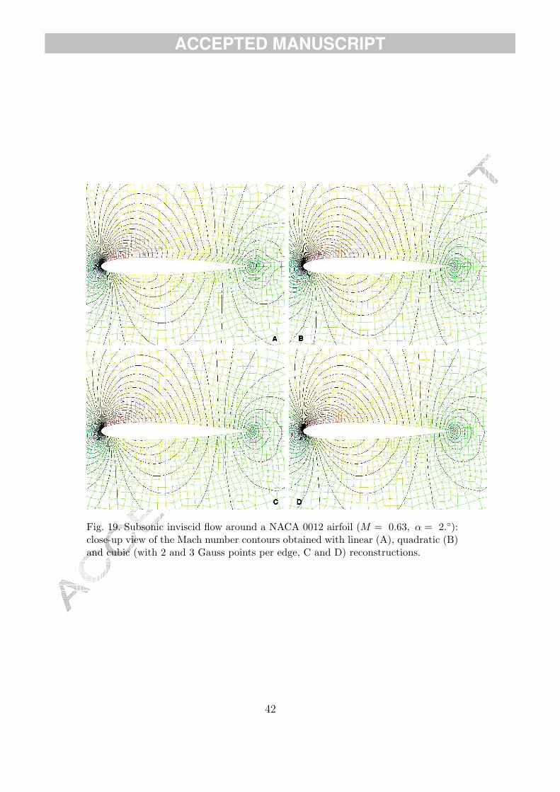
6.2.1 A subsonic test.

The problem set up corresponds to a subsonic flow around a NACA 0012airfoil. The freestream Mach number is M = 0.63 and the angle of attack isα = 2. The computational grid is rather coarse (5322 cells). Given the poormesh resolution near the leading and trailing edges, the inherent dissipationassociated to each reconstruction becomes apparent through the inspection ofthe Mach number isolines.

37

ACCEPTED MANUSCRIPT

Figure 19 presents a close-up view of the Mach number isolines obtained byusing linear (A), quadratic (B) and cubic (C and D) reconstructions. Theinviscid fluxes have been integrated using one, two and either two (C) or three(D) Gauss points per edge, for the linear, quadratic and cubic reconstructions,respectively. The solution provided by the linear reconstruction clearly showsan anomalous pseudoviscous behaviour of the Mach number contours near thesurface. The entropy layer is dramatically reduced by the increase of the orderof the reconstruction. Note that the grid was not modified near the airfoil forthe higher order schemes, and therefore straight edges are used in the boundarycells. The maximum entropy production reduces from ∆Smax = 0.03336 (linearreconstruction) to ∆Smax = 0.00772 (cubic reconstruction), where S is givenby

S = ln

h

γγ−1

p

h = γ

(E − 1

2(u2 + v2)

)(68)

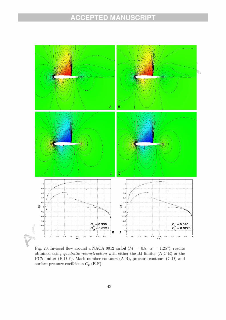
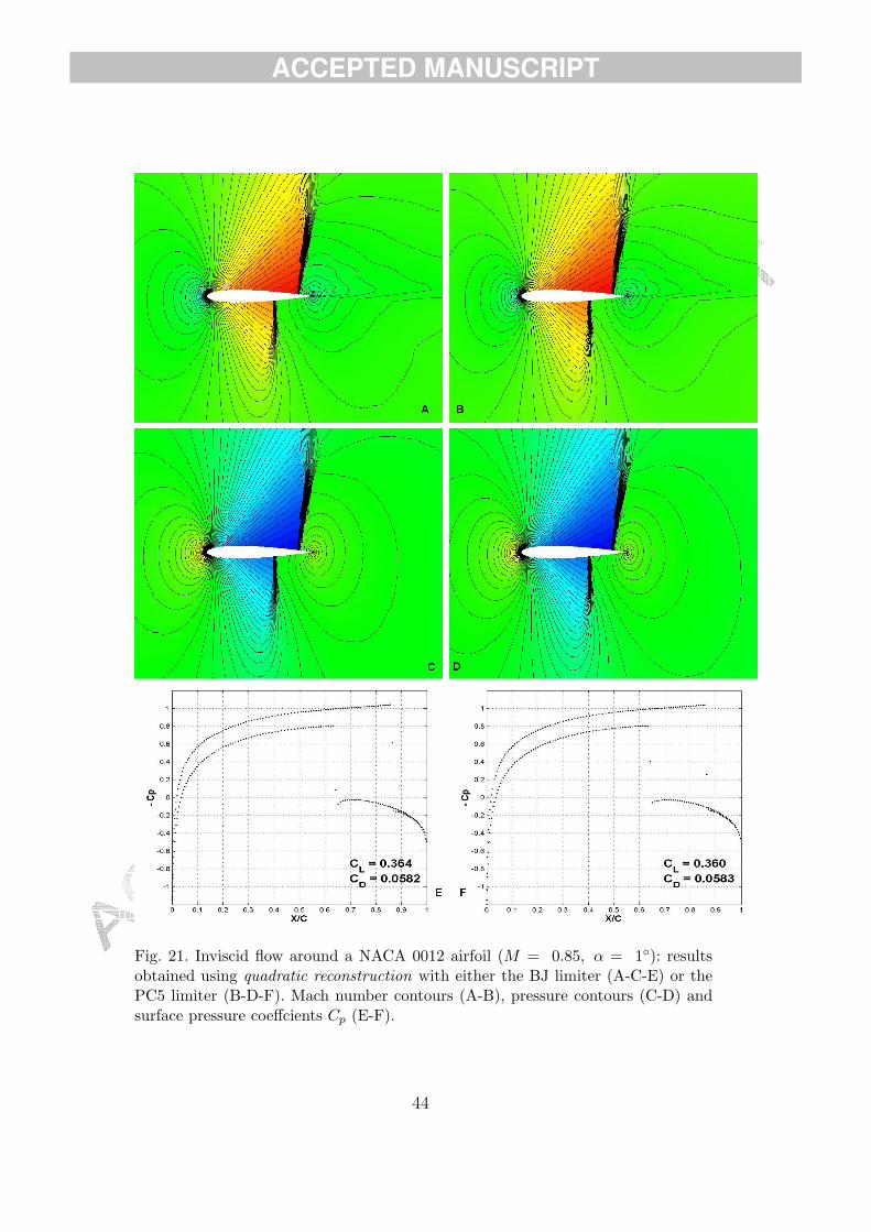
6.2.2 Two transonic examples.

A non-adapted finer grid (12243 cells) has been used to solve two transonictest cases: I) M = 0.8, α = 1.25, and II) M = 0.85, α = 1. Figures 20and 21 show the results for test cases I and II, respectively, using quadraticreconstruction and either the BJ or the PC5 limiter: Mach number isolines,pressure isolines and surface pressure coefficient Cp distribution. Both limitersprovide sharp shock-capturing (one interior cell) and clear slip lines, althoughthe PC5 limiter appears to be slightly more dissipative.

6.3 Viscous flow.

6.3.1 Shock wave impingement on a spatially evolving mixing layer.

We reproduce the example presented in [32]. An oblique shock impacts on aspatially developing mixing layer. The flow is fully supersonic at the outflow,so no explicit outflow boundary conditions are required. The problem domainis the rectangle 0 ≤ x ≤ 200 and −20 ≤ y ≤ 20, with inflow velocities specifiedas a hyperbolic tangent profile

u = 2.5 + 0.5 tanh (2y) (69)

Hence, the velocity of the upper stream is u1 = 3, whereas the velocity of

the lower stream is u2 = 2. The convective Mach number, defined asu1 − u2

c1 + c2

,

where c1 and c2 are the free stream sound speeds, is equal to 0.6.

38

ACCEPTED MANUSCRIPT

The shear layer is excited by adding a periodic fluctuation to the verticalcomponent of the velocity inflow, as

v′ =2∑

k=1

ak cos

(2πkt

T+ φk

)e

(−y2

b

)

(70)

where b = 10 and T =λ

uc

, being uc = 2.68 is the convective velocity, defined

by uc =u1c2 + u2c1

c1 + c2, and λ = 30 the wavelength. For k = 1 we take a1 = 0.05

and φ1 = 0. For k = 2, a2 = 0.05 and φ2 = π/2.

The reference density is taken as the average of the two free streams and thereference pressure is given by:

pR =(ρ1 + ρ2) (u1 − u2)

2

2(71)

Under the assumption that both streams have equal stagnation enthalpies,the local speed of sound reads

c2 = c12 +

(γ − 1)

2

(u1

2 − u22)

(72)

Equal pressure through the mixing layer is assumed. The following values areused at the inflow (left boundary)

p0 = 0.3327 H0 = 5.211 µ0 = 5× 10−4 (73)

whereas on the upper boundary we set

u = 2.9709 v = −0.1367 ρ = 2.1101 p = 0.4754 (74)

On the lower boundary, a slip wall condition was specified. With this problemsetup, an oblique shock originates from the top left corner, impacting the shearlayer around x = 90. The shock wave reflects at the lower wall and passes backthrough the deflected shear layer.

The problem was run using the fourth order scheme on two grids of 400× 100and 600 × 300 cells. Figures 22 and 23 show the contours of density (top),pressure (center) and temperature (bottom) on the fine and coarse grids, re-spectively. On both grids the fourth order scheme is capable of capturing the

39

ACCEPTED MANUSCRIPT

fine scale features of the flow, such as the formation of shocklets or the split-ting in two of the vortex core located at x = 148, caused by its interactionwith the reflected shock wave.

7 Conclusions

This paper explored the approximation power of Moving Least-Squares (MLS)approximations in the context of higher order finite volume schemes on un-structured grids. The scope of the application of MLS is threefold: 1) com-putation of high order derivatives of the field variables for a Godunov-typeapproach to hyperbolic problems or terms of hyperbolic character, 2) directreconstruction of the fluxes at cell edges, for elliptic problems or terms of el-liptic character, and 3) multiresolution shock detection and selective limiting.

A major advantage of the proposed methodology over the most popular ex-isting higher order methods is related to the viscous discretization. The useof MLS approximations allows the direct reconstruction of high order viscousfluxes using quite compact stencils, and without introducing new degrees offreedom, which results in a significant reduction in storage and workload.

A selective limiting procedure is proposed, based on the multiresolution prop-erties of the MLS approximants, which allows to switch off the limiters onsmooth regions of the flow.

Accuracy tests show that the proposed method achieves the expected conver-gence rates. Representative simulations show that the methodology is appli-cable to problems of engineering interest.

40

ACCEPTED MANUSCRIPT

Fig. 18. Shu-Osher problem, 400 cells, multiresolution-based selective limiting. Den-sity profiles computed with the third and fourth order schemes (top left and topright, respectively), high-scale components of the density (center) and detailed com-parison of the densities with and without selective limiting (bottom).

41

ACCEPTED MANUSCRIPT

Fig. 19. Subsonic inviscid flow around a NACA 0012 airfoil (M = 0.63, α = 2.):close-up view of the Mach number contours obtained with linear (A), quadratic (B)and cubic (with 2 and 3 Gauss points per edge, C and D) reconstructions.

42

ACCEPTED MANUSCRIPT

Fig. 20. Inviscid flow around a NACA 0012 airfoil (M = 0.8, α = 1.25): resultsobtained using quadratic reconstruction with either the BJ limiter (A-C-E) or thePC5 limiter (B-D-F). Mach number contours (A-B), pressure contours (C-D) andsurface pressure coeffcients Cp (E-F).

43

ACCEPTED MANUSCRIPT

Fig. 21. Inviscid flow around a NACA 0012 airfoil (M = 0.85, α = 1): resultsobtained using quadratic reconstruction with either the BJ limiter (A-C-E) or thePC5 limiter (B-D-F). Mach number contours (A-B), pressure contours (C-D) andsurface pressure coeffcients Cp (E-F).

44

ACCEPTED MANUSCRIPT

Fig. 22. Shock wave impingement on a mixing layer at t = 120. Fourth order resultson the 600×300 grid. Contours of density (top), pressure (center) and temperature(bottom).

45

ACCEPTED MANUSCRIPT

Fig. 23. Shock wave impingement on a mixing layer at t = 120. Fourth order resultson the 400×100 grid. Contours of density (top), pressure (center) and temperature(bottom).

46

ACCEPTED MANUSCRIPT

8 Acknowledgements

This work has been partially supported by the “Ministerio de Educacion yCiencia” of the Spanish Government (grants #DPI2004-05156 and #DPI2006-15275) cofinanced with FEDER funds, and by the “Xunta de Galicia” (Grants# PGIDIT05PXIC118002PN and # PGDIT06TAM11801PR).

The research of Dr. Luis Cueto-Felgueroso is supported by the “Ministerio deEducacion y Ciencia” through its program of postdoctoral scholarships. Fur-thermore, it is also gratefully acknowledged the financial support received inthe past from “Colegio de Ingenieros de Caminos, Canales y Puertos”, “Fun-dacion de la Ingenierıa Civil de Galicia” and “Caixanova” . Mr. Xesus Nogueiragratefully acknowledges the financial support received from “Fundacion CaixaGalicia”.

References

[1] B. Cockburn, C.W. Shu. Runge-Kutta Discontinuous Galerkin methods forconvection-dominated problems. Journal of Scientific Computing. 6:173-261(2001).

[2] Z.J. Wang, L. Zhang, Y. Liu. Spectral (finite) volume method for conservationlaws on unstructured grids IV: extension to two-dimensional Euler equations.Journal of Computational Physics. 194:716-741 (2004).

[3] P. Lancaster, K. Salkauskas. Surfaces generated by moving least squaresmethods. Math. of Comp. 155:141–158 (1981).

[4] W.K. Liu, S. Li, T. Belytschko. Moving least-squares reproducing kernelmethods: (I) Methodology and Convergence. Computer Methods in AppliedMechanics and Engineering. 143:113–154 (1997).

[5] S. Li, W.K. Liu. Moving least-squares reproducing kernel methods: (II) Fourieranalysis. Computer Methods in Applied Mechanics and Engineering. 139:159–193 (1996).

[6] S. Li, W.K. Liu. Reproducing kernel hierarchical partition of unity, part I- Formulation and theory. International Journal for Numerical Methods inEngineering. 45:251–288 (1999).

[7] A. Gossler. Moving Least-Squares: a numerical differentiation method forirregularly spaced calculation points. SANDIA Report, SAND2001-1669 (2001).

[8] D. Levin. The approximation power of moving least-squares. Mathematics ofComputation. 67(224):1517-1531 (1998).

47

ACCEPTED MANUSCRIPT

[9] L. Cueto-Felgueroso, I. Colominas, J. Fe, F. Navarrina, M. Casteleiro. Highorder finite volume schemes on unstructured grids using Moving Least-Squaresreconstruction. Application to shallow water dynamics. International Journalfor Numerical Methods in Engineering. 65:295-331 (2006).

[10] S.K. Godunov. A difference method for the numerical calculation ofdiscontinuous solutions of hydrodynamic equations. Mat. Sbornik. 47(3):271-306 (1959).

[11] A. Harten, P. Lax, B. Van Leer. On upstream differencing and Godunov-typeschemes for hyperbolic conservation laws. SIAM Rev. 25:35-61 (1983).

[12] T.J. Barth, D.C. Jespersen. The design and application of upwind schemes onunstructured meshes. AIAA-89-0366 (1989).

[13] N.T. Frink. Upwind scheme for solving the Euler equations on unstructuredtetrahedral meshes. AIAA J. 30(1):70 (1992).

[14] V. Venkatakrishnan. Convergence to steady state solutions of the Eulerequations on unstructured grids with limiters. Journal of ComputationalPhysics. 118:120–130 (1995).

[15] P. Jawahar, H. Kemath. A high-resolution procedure for Euler and Navier-Stokes computations on unstructured grids. Journal of Computational Physics.164:165–203 (2000).

[16] T.J. Barth. Aspects of unstructured grids and finite-volume solvers for the Eulerand Navier-Stokes equations. VKI Lecture Series 1994-05.(1995).

[17] J.M. Vaassen, P Wautelet, J.A. Essers. A quadratic reconstruction scheme forhypersonic reacting flows on unstructured meshes. ECCOMAS ComputationalFluid Dynamics Conference. Swansea, Wales, UK (2001).

[18] I. Aavatsmark. An introduction to multipoint flux approximations forquadrilateral grids. Computational Geosciences. 6:405-432 (2002).

[19] W.K. Liu, W. Hao, Y. Chen, S. Jun, J. Gosz. Multiresolution reproducing kernelparticle methods. Computational Mechanics. 20:295-309 (1997).

[20] B. Sjogreen, H.C. Yee. Multiresolution wavelet based adaptive numericaldissipation control for high order methods. Journal of Scientific Computing.20:211-255 (2004).

[21] F.M. White. Viscous fluid flow. (2nd edition) McGraw-Hill. New York (1991).

[22] L. Cueto-Felgueroso, I. Colominas. High-order finite volume methods andmultiresolution reproducing kernels. Archives of Computational Methods inEngineering. Submitted.

[23] L. Cueto-Felgueroso. Particles, finite volumes and unstructured grids: numericalsimulation of fluid dynamics problems. PhD Thesis (in Spanish). Universidadde A Coruna (2005). (http://www.tesisenred.net/)

48

ACCEPTED MANUSCRIPT

[24] L. Cueto-Felgueroso, I. Colominas, G. Mosqueira, F. Navarrina, M. Casteleiro.On the Galerkin formulation of the SPH method. International Journal forNumerical Methods in Engineering. 60:1475–1512 (2004).

[25] B. van Leer. Towards the ultimate conservative difference scheme V. A secondorder sequel to Godunov’s method. Journal of Computational Physics. 32:101(1979).

[26] J. Van Rosendale. Floating shock fitting via Lagrangian adaptive meshes.ICASE 94-89 (1989).

[27] G. D. Van Albada, B. Van Leer, W. W. Roberts. A comparative study ofcomputational methods in cosmic gas dynamics. Astronomy and Astrophysics108: 76 (1982).

[28] P.L. Roe. Approximate Riemann solvers, parameter vectors and differenceschemes. Journal of Computational Physics. 43:357–372 (1981).

[29] C.-W. Shu, S. Osher. Efficient implementation of essentially non-oscillatoryshock-capturing schemes. Journal of Computational Physics. 77:439-471 (1988).

[30] A.H. Shapiro. The dynamics and thermodynamics of compressible fluid fow.Ronald Press Co. New York (1953).

[31] C.W. Shu, S. Osher. Efficient implementation of essentially non-oscillatoryshock-capturing schemes, II. Journal of Computational Physics. 83:32-78(1989).

[32] H.C. Yee, N.D. Sandham, M.J. Djomehri. Low-dissipative high-order shock-capturing methods using characteristic-based filters. Journal of ComputationalPhysics. 150:199-238 (1999).

49