accelerating the convergence of multiphase flow

J. Appl. Comput. Mech., 7(1) (2021) 235-253 DOI: 10.22055/JACM.2020.35096.2563

ISSN: 2383-4536 jacm.scu.ac.ir

Published online: November 12 2020

Accelerating the Convergence of Multiphase Flow Simulations

when Employing Non-Uniform Structured Grids

Gautham Krishnamoorthy1 , Lauren Elizabeth Clarke1,2 , Jeremy Nicholas Thornock3

1 Department of Chemical Engineering, UPSON II Room 365, 241 Centennial Drive, University of North Dakota,

Grand Forks, ND 58202-7101, USA, Email: [email protected] 2 Department of Chemical Engineering, Massachusetts Institute of Technology, 77 Massachusetts Avenue, Room 66-350, Cambridge, Massachusetts 02139, Email: [email protected]

3 Department of Chemical Engineering, 50 S. Central Campus Dr., Room 3290 MEB, University of Utah, Salt Lake City, UT 84112-9203, USA, Email: [email protected]

Received September 19 2020; Revised November 11 2020; Accepted for publication November 11 2020.

Corresponding author: G. Krishnamoorthy ([email protected])

© 2020 Published by Shahid Chamran University of Ahvaz

Abstract. Non-uniform grids inevitably arise in multiphase flow simulation scenarios due to the need to resolve near-wall phenomena and/or large L/D ratios associated with the reactor configuration. This in conjunction with large density ratios of the constituent phases can retard the convergence of the pressure-correction equation that results from applying operator-splitting methods to the incompressible Navier-Stokes equations. Various pre-conditioning strategies to this ill-conditioned pressure-correction matrix are explored in this study for a class of bubbling bed simulations encompassing: different particle densities, bed-heights and dimensions (2D/3D). The right-side Block Jacobi preconditioning option resulted in a 20 - 35% decrease in CPU time that correlated well with a decrease in the number of iterations to reach a specified tolerance.

Keywords: PETSc; MFiX; BiCGSTAB; Preconditioner; Multiphase flow.

1. Introduction

Multiphase CFD simulation scenarios present a number of additional challenges beyond those present in single-phase simulations. Among these are: large constituent density ratios, presence of discrete interfaces, significant mass transfer rates, non-equilibrium interfacial dynamics along with the fact that they are inherently transient in nature [1]. In the Two-Fluid Model (TFM) framework for simulating multiphase flows, the governing equations for all the phases involved are solved in an Eulerian framework and the coupling between the different phases is achieved through an appropriate modeling of the interaction and source terms in the respective phase equations. A solution to the incompressible Navier Stokes equation for the different phases is then undertaken using operator-splitting methods where a pressure-correction equation is formulated implicitly, requiring the solution of a linear system at each time step. Using the extended SIMPLE algorithm developed by Syamlal [2], the pressure-correction equation takes the form of a discrete Poisson equation with discontinuous coefficients. The solution to this equation consumes the bulk of the computational time in multiphase simulations because density is a coefficient in the pressure-correction equation and large variations or discontinuities among the phase densities greatly increase the condition number of the pressure-correction matrix and retard the convergence of iterative methods employed in its solution [3, 4]. Further, non-uniform grids inevitably arise in various multiphase flow simulation scenarios due to the need to accurately resolve near-wall phenomena. For instance, stretched, large-aspect ratio grids near the boundary wall are employed in multiphase modeling of: particle deposition [5], cloud cavitation near air foils [6] and multiphase heat transfer in microchannels [7]. In other instances, large L/D ratios associated with the reactor configuration such as those found in solid sorbent systems [8] and circulating fluidized beds [9] may result in the generation of non-uniform or high-aspect ratio cells where cells are stretched in the direction of the dominant velocity vector to minimize the computational simulation cost. Finally, the study of multiphase hydrodynamics in complex geometries such as: resolving the air core accurately in hydro cyclones [10], studying the erosion and heat transfer characteristics of tube bundles immersed in fluidized beds [11] or the cavitation characteristics in centrifugal pumps [12] may naturally result in the generation of non-uniform grids along with sudden changes to cell aspect ratios. It is well known that the iterative convergence of many solution methods, rapidly deteriorate when applied on non-uniform [13 - 14] and high-aspect ratio grids [15]. The performance degradation has been seen to be even more severe in parallel computing environments especially when the grid is decomposed along the direction where the cell aspect ratio is high [16]. The primary goals of this manuscript are to:

1. Highlight for the first time, this degradation in the convergence of iterative methods when employing non-uniform structured grids in multiphase flow simulations encompassing different: particle densities, bed-heights, jet inlet velocities, problem dimensions (2D/3D) and grid types (uniform/non-uniform) in a bubbling bed configuration.

2. Propose a remedy to this convergence degradation through the judicious selection of pre-conditioner (PC) to Krylov Subspace (KSP) iterative solvers.

By working within the framework of the open-source multiphase simulation code MFiX [17], we first interface it with the robust,

236 Gautham Krishnamoorthy et. al., Vol. 7, No. 1, 2021

Journal of Applied and Computational Mechanics, Vol. 7, No. 1, (2021), 235-253

scalable PETSc linear solver library [18] through an appropriate mapping of the matrix and vector data structures between the two software frameworks. Through this interface an access to a wide range of solver and PC options in PETSc was then obtained with the additional option of applying the preconditioning strategy from the left-side (which is more common) as well as the right side. By keeping the KSP method fixed (BiCGSTAB) throughout our analysis, a performance assessment of the different PC’s is made by comparing against the default line preconditioning option in the native MFiX solver by allowing all options to converge to the same residual tolerance.

The PETSc [18] library allows for the transparent use of various Krylov subspace solvers and preconditioner options in large-scale parallel environments without the need to write specialized code to access them. Our emphasis on identifying the correct PC is driven by the studies of Zhang [19] and Ghai et al. [20] who demonstrated that when utilizing preconditioned KSP methods, the choice of the preconditioners employed in the preconditioned iterative solvers determine the overall convergence rate of the iteration procedure. By carefully evaluating a wide range of non-symmetric matrix systems arising from CFD simulations, the authors [19, 20] reinforced the current consensus among preconditioning technique practitioners that the quality of the preconditioner is more critical than the choice of the Krylov subspace accelerator in designing a preconditioned iterative solver for large scale CFD applications. The MFiX-PETSc interfaces was developed in a “black box” fashion after an appropriate mapping of matrix and vector data structures between the CFD code and linear solver libraries as shown in Figure 1.

This means, the coefficients for the matrix and right hand side vector are first passed on to PETSc. PETSc then use these coefficients to create the global matrix and vectors. Once the solve is completed and the solution vector passed back to MFiX, the global matrix and vectors are thrown away only to be created again on the subsequent time-step. Verification of the implementation of our MFiX-PETSc framework was carried out by comparing our numerical predictions of a steady-state heat conduction problem (TFM01) and a single phase plane Poiseuille flow problem (TFM02) both of which have known analytical solutions (not discussed in this paper) [21].

2. Method

2.1 Governing Equations

For the isothermal, non-reacting systems investigated in this study, the continuity equation for the fluid and solids phases in the Two-Fluid Model (TFM) in MFiX can be represented respectively as follows [22]:

�� + �

�� = ��

��

�� (1)

�� + �

�� = ��

��

�� (2)

where �� is the fluid volume fraction, �� is the volume fraction of the �� solids phase, �� is the fluid-phase density, �� is the density of the �� solids phase, �� is the �� velocity component of the fluid-phase, and �� is the �� velocity component of the �� solids phase. The right-hand term denotes interphase mass transfer due to chemical reactions or other physical phenomena. The corresponding momentum equations for the fluid phases are represented as [22]:

�� + �

�� = −��

��

+ ��

+ �ℛ�� − ℛ�� − ��!"

��+ #�� + ��$� (3)

where �� is the fluid-phase pressure, �� is the stress tensor of the fluid-phase, ℛ�� is mass transfer from the fluid-phase to the �� solids phase, ℛ�� is mass transfer from the �� solids phase to the fluid-phase, �� represents momentum transfer between the fluid and the �� solids phase caused by interphase forces (such as the drag force), #�� is fluid flow resistance due to porous media, and $� is acceleration due to gravity. The momentum balance for the solids phase is represented similarly as [22]:

�� %��& + �

�� = −��

��

− ��'��

+ ��

+ (ℛ)�)� − ℛ�)�� − �)�*"

��+ ��$� (4)

where �' is solids-phase pressure in close packed regions (which uses an equation of state to increase this term exponentially to constrain the solid volume fractions to their close packing limit), �� is the stress tensor of the �� solids phase, ℛ)� is mass transfer from the +�� phase to the �� phase, ℛ�) is mass transfer from the �� phase to the +�� phase, and �)� represents momentum transfer between the �� phase and the +��phase caused by interphase forces (such as the drag force).

MFiX applies the finite volume method with a staggered grid to discretize the governing equations. Using this approach, scalar values (i.e. fluid-pressure) are computed at the center of the control volume whereas velocity components are calculated along the faces of the control volume. An interpolation scheme (section 2.4) is required to interpolate the face-centered velocities to their cell–centered values. After this is accomplished, discretization of scalar transport equations for all phases can be represented as [22]:

%,�&-%ф�&- = %,�&�/%ф�&�/ +�/

0� + 12 3),�

"

)�5(%ф)&- − %ф�&-* (5)

Fig. 1. A block diagram of the matrix and vector mapping associated with the MFiX-PETSc interface for solving the linear matrix equation Ax = b.

Accelerating the Convergence of Multiphase Flow Simulations 237


In equation (5), the coefficient , contains flow properties and geometric parameters from the discretized equations (including phase volume fractions, densities, velocities and cell surface areas), ф is a given scalar value, 0 is a source term, and 3),� is the interface transfer coefficient. Subscript 6 represents the phase, subscript � is the central point of the scalar quantity undergoing calculation, and subscript 60 denotes its neighbor central points (E, W, N, S, T, and B).

2.2 Numerical Method

When flow is incompressible, challenges arise in computing the fluid flow field. As shown in Eqs. (1) through (4), there is a strong, implicit coupling between the pressure and velocity fields. In MFiX, the solids phase pressure is resolved with a volume fraction correction equation and the fluid-phase pressure field is resolved with a fluid-pressure correction equation [22] using the SIMPLE algorithm. The SIMPLE algorithm is an operator-splitting numerical procedure that is widely employed in CFD to solve the discretized Navier-Stokes equations for incompressible systems. MFiX employs a version of the SIMPLE algorithm developed by Patankar [23] that has been extended to multiphase systems. This involves the solution to a fluid-pressure correction equation to satisfy continuity and then update the gas pressure and velocity fields.

If the intermediate values for pressure and velocity from solving the momentum equations are represented by P* and u* respectively. Then, the relationship between the intermediate value (ф*) and the actual value (ф) for these parameters (that also satisfies the continuity equation) is denoted as ф = ф* + ф’, where ф’ is the correction value. Derivation of the fluid-pressure correction equation first requires replacing pressure (P) and velocity (u) terms in the discretized fluid-phase momentum equation with intermediate pressure (P*) and velocity (u*) terms. Then, the P* = P – P’ and u* = u – u’ expressions are substituted into this equation. The original discretized gas momentum equation, with actual pressure and velocity values, is subtracted to yield an expression only containing velocity (u’) and pressure (P’) correction terms. The resultant fluid-pressure correction equation is then of the form [2]:

78�998: �9 = 78�;<98: �;< +;<

<8 (6)

In stencil based codes such as MFiX, Eq. (6) results in a symmetric septa-diagonal matrix. However, due to the manner in which boundary cells are treated in MFiX, the resulting matrix ends up being non-symmetric. The pressure correction terms calculated using Eq. (6) are then used to calculate the actual gas-phase pressure [2]:

98�9 = 98∗ � + >9898: �9 (7)

for which >98 is a relaxation factor. This pressure correction is also used to update the gas-phase velocity [2]:

?8�@ = ?8∗ �@ + A8�@ B98: �9 − 98: �CD (8)

where A8 is an interphase mass transfer factor. As noted in Eq. 6 the coefficients ag are a function of: phase densities, phase volume fractions, phase velocities and geometric

surface areas. Sudden changes in these values across neighboring cells can increase the condition number of the pressure correction matrix (Eq. 6) and retard the convergence of iterative methods employed in its solution. The goal of this manuscript is to highlight and address these deficiencies.

This is undertaken by comparing the CPU times and the number of iterations taken by different solver – PC options to reach a specified tolerance during the solution to Eq. (6). This is denoted as the number of inner iterations in this study.

In the transient simulations undertaken in this study, MFiX uses an automatic time step adjustment to reduce the run time. This is done by making small upward or downward adjustments in time steps and monitoring the total number of outer iterations for several time steps. The adjustments are continued, if there is a favorable reduction in the number of outer iterations per second of simulation. Otherwise, adjustments in the opposite direction are attempted. Differences in the solver-PC options employed in the simulation may result in slight changes to the time-step sizes during the course of the simulation. Therefore, to compare the performances of different solvers and PC, the total number of inner iterations taken to reach a specified simulation time were also monitored.

2.3 Iterative Solvers and Pre-Conditioners

MFiX offers four iterative methods and two preconditioners (line and diagonal) to then solve the system of equations described in section 2.2. Among these, the BiCGSTAB iterative solver with the line-preconditioning option have been deemed to be the fastest solver-PC option for a wide range of multiphase flows [2]. By interfacing MFiX with PETSc, we were able to obtain access to a wider range of Krylov Subspace Solvers and Preconditioners. The steps involved during the use of the MFiX - PETSc solver interface for solving the generic linearized system, EF = < shown in Figure 1 involves: 1. Problem Setup: Functionality for setting PETSc solver parameters such as solver tolerances, maximum number of iterations,

and preconditioners as dictated by derived solver types. 2. Solver Setup: Solver object creation (allocation of E, F, and <) and initialization. 3. Communication Linear System: Handshake function for passing the linear system coefficients (E) and right-hand-side values

(<) in the current native MFiX data-structure and subsequent conversion to the solver-specific types for PETSc. 4. Solve System: Using PETSc’s native solver types, this function will compute the solution (F) to the linear system. 5. Return/Copy Solution: Conversion of the solver type solution (F) to the current, native MFiX type. 6. Cleanup: De-allocation and destruction of PETSc solver objects.

While solving the linear system (step 4) is likely to consume the majority of the computational time, a slight overhead cost associated with the solver object creation (step 2) is also to be expected and is also investigated in this study.

Since the goal of this study is to assess the degradation in the convergence of iterative methods when employing non-uniform structured grids in multiphase flow simulations encompassing different: particle densities, bed-heights, jet inlet velocities, problem dimensions (2D/3D) and grid types (uniform/non-uniform) and suggest remedies, the line preconditioning option in conjunction with the BiCGSTAB solver was used throughout this study when employing the native MFiX solver. Additionally, the Block Jacobi PC option was employed with the MFiX-PETSc framework. This has previously been deemed to be the fastest PC option in the MFiX – PETSc framework for a wide class of flows during the software verification process where numerical predictions of a steady-state heat conduction problem (TFM01) and a single phase plane Poiseuille flow problem (TFM02) were compared against known analytical solutions [21, 24].

For a linear system containing a non-symmetric matrix, a preconditioner can be applied from the left- or right-side. In general, application of a preconditioner from the left to a linear system will yield [25]:



Fig. 2. Dimensions and the grid associated with the thin rectangular fluidized beds investigated in this study; (a) Dimensions along the x- and y- directions; (b) The non-uniform grid which is well resolved near the jet center; (c) The 3D uniform grid with an initial bed height of H/D = 2.

GHIEF = GHI< (9)

where G is the preconditioning matrix. Preconditioning performed from the right is of the form [25]:

EGHI? = < (10)

where F = GHI?. While it is true that left- and right-side preconditioners have similar asymptotic behavior, they can actually behave differently

depending on the linear system. The termination criterion of Krylov subspace methods is generally related to the residual norm of the preconditioned system. When preconditioning is applied from the left, the preconditioned residual, defined as JGHIKLJ, can

greatly differ from the true residual JKLJ if the ‖GHI‖ value is far from 1. Unfortunately, this can be a common problem when applying left preconditioning to large linear systems. On the other hand, right preconditioners use the unaltered, true residual with an insignificant increase in computational cost. Right preconditioners should not lead to large solution errors, unless the preconditioning matrix, G , is extremely ill-conditioned [20]. In a similar vein, Tadano and Sakurai [26] have shown that the perturbation of a preconditioner does not affect the accuracy of an approximate solution with right side preconditioning.

Block Jacobi preconditioners are methods of block preconditioning geared towards parallel environments. Traditional Block Jacobi preconditioning employs a domain decomposition with no overlap. The Block Jacobi preconditioners in PETSc are obtained by applying incomplete LU factorizations with zero-fill in (ILU(0)) on each processor’s local diagonal blocks. In general, the ILU factorization process formulates a sparse lower triangular matrix O and a sparse upper triangular matrix P which have the same nonzero structure as the lower and upper sections of E. These matrices are computed so that Q = OP − E, the residual matrix, satisfies a certain constraint. For the ILU(0) method, this constraint is having zero entries in certain locations. This technique aims to define a preconditioner G = OP such that the elements of the residual matrix are zero in the locations that the E matrix is non-zero [25]. In this study, since the preconditioner is applied in a serial context, the Block Jacobi preconditioner is actually an ILU(0) preconditioner. Most methods of solving a given linear system, EF = <, include passing through iterations by altering one or more components of an approximate vector solution at each iteration. By default, both PETSc and MFiX test for convergence based upon the RS-norm (‖KT‖S) of the preconditioned residual (KT). In PETSc, convergence is detected at iteration T if [18]:

‖UV‖S < XYZ%U[\] ∗ ‖^‖S, Y[\]& (11)

where KT = < − EFT, K_`R is the decrease of the residual norm relative to the norm of the right hand side, 7_`R is the absolute size of the residual norm, and A_`R is the relative increase in the residual. The K_`R, 7_`R, and A_`R parameters can be set by the user.

2.4 Discretization Schemes for the Convection Terms

When flows are transient, multi-dimensional, or contain strong sources, higher-order discretization schemes for convection can help increase accuracy, but they can also create issues with overshoots and undershoots near discontinuities, known as oscillations. This can create problems with convergence and physically unrealistic intermediate solutions [2]. Total variation diminishing (TVD) schemes have been developed to resolve discontinuities without producing these oscillations. These techniques employ a limiter which bounds the value of ф (velocity) using the notations for the node locations that are based on the flow direction. The notation D represents downwind, U represents Upwind, C is the central point of the control volume, and f is the face of the control volume. The limiter is expressed as a function of the normalized value of ф, which is defined as [2]:

фa = ф − фPфb − фP

. (12)



Table 1. List of material properties and some of the modeling parameters

Material Glass Polypropylene

Density (kg/m3) 2545 900

Coefficient of Restitution 0.9 0.6

Angle of Internal Friction 30˚ 30˚

Diameter (μm) 425 425 Minimum Fluidization Velocity (m/s) 0.30 0.11 Drag Coefficients (drag_C1, drag_D1) 0.771, 2.8781 0.641, 4.0144

Table 2. A Summary of numerical parameters employed in the 2D simulations to study the effects of grid uniformity.

Bed Height (Grid Type)

Dimensions Mesh

(Total # cells) Time Step (sec) Tolerance Vjet Solver

Discretization Scheme

PC

H/D = 2 (Non-Uniform) 20x100 cm2

56x250 (14,000) Max: 1e-03

Min: 1e-06

Outer 1e-03

Solver 1e-03

5 m/s

BiCGStab

van Leer

MFiX Line

MFiX-PETSc BJACOBI (left)

MFiX-PETSc BJACOBI (right)

H/D = 2 (Uniform) 20x100 cm2

40x200 (8,000)

Table 3. A Summary of numerical parameters employed in the 2D simulations to study the effects of bed height.


Dimensions Mesh

(Total # cells) Time Step (sec) Tolerance Vjet Solver

Discretization Scheme

PC

H/D = 1 (Non-Uniform)

20x100 cm2 56x250 (14,000)

Max: 1e-03 Min: 1e-06

Outer 1e-03

Solver 1e-03

5 m/s

BiCGStab

van Leer

MFiX Line



H/D = 2 (Non-Uniform)

20x100 cm2 56x250 (14,000)

Table 4. A Summary of numerical parameters employed in the 3D simulations to study the effects of grid uniformity.


Dimensions Mesh

(Total # cells) Tolerance Time Step (sec) Vjet Solver Scheme PC

H/D = 2 (Non-Uniform) 20x100x2 cm3

56x100x2 (11,200)

Outer: 1e-02 Solver:

1e-03 (Glass), 1e-02 (Polypropylene)

Max: 1e-03 Min: 1e-06

5 m/s

BiCGStab

van Leer van Leer

MFiX Line



H/D = 2 (Uniform) 20x100x2 cm3

40x200x4 (32,000)

Outer: 1e-03 Solver: 1e-03

TVD schemes bound ф with this limiter when the variation in ф is monotonic, which occurs when d ≤ фaf ≤ I. A down-wind

factor formulation for discretization, proposed by Leonard and Mokhtari [27], has been adopted into the TVD schemes implemented in several existing codes due to its ability to retain the traditional septa-diagonal matrix structure in linear systems. However, TVD schemes differ by how they calculate the down-wind weighting factor. In the van Leer scheme, the down-wind factor is equal to фfg [2] and is the scheme adopted in this study.

3. Results and Discussion

The fluidized bed cases for assessing the performances of the different PC explored in this study is based on the experimental and computational study of Utikar and Ranade [29]. Their experimental set up consisted of a 3-dimensional, thin rectangular fluidized-bed operated with a central jet. Their study examined the fluidization characteristics of glass and polypropylene particles at two bed heights (H/D = 1, 2) and three different jet inlet velocities (Vjet) of: 5 m/s, 10 m/s, and 20 m/s. The advantages of thin rectangular fluidized beds include the ability to perform detailed optical diagnostics for obtaining high quality data for validating numerical simulations. Further, highly resolved 2D simulations of these reactor geometries may enable the development/tuning of multiphase sub-models parameters and facilitate conducting parametric studies for design and scale up at a reduced computational cost.

In order to isolate the effects of bed height and particle densities on the iterative solve time, the first set of simulations in this study employed a jet inlet velocity (Vjet) of 5 m/s. In addition, the simulations were carried out in both 2D and 3D domains using uniform as well as non-uniform meshes to assess the performances of PC in solving penta-diagonal (2D) as well as septa-diagonal (3D) matrix systems. The dimensions and the grids employed in this study are shown in Figure 2.

For the drag model, we employed the Syamlal – O’Brien drag model parameters with the coefficients modified to match the minimum fluidization velocities of glass (0.3 m/s) and polypropylene (0.11 m/s). A list of the material properties and the modeling parameters pertinent to this study are reported in Table 1.

Summaries of numerical parameters employed in the 2D simulations to study the effects of grid uniformity and bed-height are shown in Tables 2 and 3 respectively.

In the uniform grids, the mesh resolution is 11.8 times the particle diameter, whereas in the non-uniform grids, the mesh do not have an aspect-ratio of 1. Nevertheless, the mesh resolution (considering the larger of the mesh dimensions) varies between 9.4 (in the highly resolved central region) to 23.5 times the particle diameter. Although the focus of this paper is on assessing the numerical convergence of different PC, it is still worth noting that a grid resolution of 18 times the particle diameter have been deemed as adequate for obtaining grid-independent results when simulating the hydrodynamics of Geldart B particles (the particle type chosen in this study) [30]. Table 4 summarizes the numerical parameters employed in the 3D simulations to study the effects of grid uniformity.



Fig. 3. Typical fluidization behavior (contours of gas volume fraction Ep_g) observed with the Polypropylene particles in the 2D simulations

(H/D = 2)

Fig. 4. Typical fluidization behavior (contours of gas volume fraction Ep_g) observed with the Glass particles in the 2D simulations (H/D = 2).

Slight increases to the solver and outer iteration tolerances (from their default values of 1e-03 employed throughout this study) were necessary in the 3D non-uniform grid simulations due to divergence of select solver-PC combinations. The tolerances shown in Table 4 are the ones in which all three solver-PC combinations could run successfully for 20 seconds to ensure consistency when comparing the different PCs.

3.1 Comparison of Fluidization Characteristics

The typical fluidization characteristics of the polypropylene and glass particles at a bed height of H/D = 2 are shown through the contours of gas-phase volume fraction (Ep_g) in Figures 3 and 4 respectively.

These snapshots are at around 12 seconds of simulation time after the initial transient characteristics associated with the initial conditions have been washed away. While the general fluidization characteristics are identical between: the uniform and non-uniform grid simulations as well as between the different solver – PC options, the contours do not evolve in an identical manner among the different options. During a transient simulation, initial differences among the solvers can be amplified as a result of the variable time-stepping algorithm employed in MFiX. When transient results start to differ, the number of iterations per time step start to vary resulting in the time steps being adjusted at a different rate. In fact, previous studies have observed these discrepancies to arise even due to differences in the Fortran compilers employed to make the MFiX executable [31]! The general fluidization characteristics shown in Figures 3 and 4 are in general agreement with the experimental images reported in Utikar and Ranade [29]. In case of glass beads (Figure 4), bubbles are formed immediately close to the distributor whereas for Polypropylene particles, a jet is seen before the formation of bubbles. Further, in the case of polypropylene particles, the jet and bubbles do not rise vertically but rather move throughout the column as observed in the experiments. The general fluidization characteristics of the simulations remain unchanged as a result of the different PC options.

Figures 5 and 6 show the time-averaged and standard deviation of the pressure drop across the bed over 10 seconds of simulation time (from 10 – 20 seconds) in the 2D and 3D simulations respectively. The time-averaged pressure drops remain unchanged with the different PC options across all the simulation scenarios.



Fig. 5. Average and standard deviation of the pressure drop across the bed over 10 seconds of simulation time (from 10 – 20 seconds) in the 2D simulations (all results are from employing a non-uniform mesh unless explicitly mentioned): (a) Effect of bed height (Glass beads); (b) Mesh type

(Glass beads); (c) Effect of bed height (Polypropylene beads); (b) Mesh type (Polypropylene beads).

Fig. 6. Average and standard deviation of the pressure drop across the bed over 10 seconds of simulation time (from 10 – 20 seconds) in the 3D simulations (all results are from employing a non-uniform mesh unless explicitly mentioned): (a) Mesh type (Glass beads); (b) Mesh type

(Polypropylene beads).



Fig. 7. Power spectral density plots of the pressure fluctuations (from 10 – 20 seconds) from the simulations performed on non-uniform mesh.

(Straight lines corresponding to the decay in power spectrum with a slope of -4 are also shown).

The dynamic characteristics of the simulations were compared next using power spectral density (PSD) plots of the pressure fluctuations (obtained at 15 mm above the jet inlet) over 10 seconds of simulation time and are shown in Figure 7 (Non-Uniform mesh).

On log-log plots, the power-law decay of the PSD of pressure fluctuations across all simulations are seen to have slopes close to -4 in agreement with experimental observations in this configuration [29] as well as other bubbling fluidized beds [32]. However, differences in solver-PC combinations sometimes resulted in differences in the identification of the dominant frequencies of the pressure fluctuations as reported in Table 5.

As seen in Figure 7d, where a distinct peak associated with the PSD is seen, in Figures 7a – c, several peaks of similar magnitudes are observed. It is possible that obtaining pressure samples over an extended period of time (> 10 seconds) would lead to a more accurate identification of the dominant frequency characteristics [33, 34].

3.2 Solver-PC Performance Comparisons in 2D Simulations

Figure 8a shows the CPU time ratios relative to that of the native MFiX solver (i.e., MFiX-PETSc CPU time/native MFiX CPU time) to simulate 20 seconds of fluidization in 2D. On uniform grids, the MFiX’s native solver – PC options perform better than the MFiX – PETSc PC options.

On non-uniform grids however, the use of right side BJACOBI PC results in 30 -35% solution speed-up compared to MFiX. Further, the right side PC performs better than the more commonly used left side PC option. Since the solution to the pressure-correction equation often limits the rate of convergence, the average and standard deviation of the number of pressure solve iterations over 20 seconds of simulation time are shown in Figure 8b. On non-uniform grids, the BJACOBI PC options take less iterations to converge to the specified tolerance and thereby cause the CPU times to be lower than those of the native MFiX solver. Further, when moving from uniform to non-uniform grids while the average number of solver iterations increases across all PC options, the change is greatest for MFiX’s line PC and the least with the BJACOBI (right) PC indicative of its robustness with an increase in problem size as well as condition number. Figure 9 shows the total number of time steps and the total number of inner iterations for the pressure solve over 20 seconds of simulation time.

Table 5. The dominant frequency (in Hz) of the pressure fluctuations (from 10 – 20 seconds) in the simulations performed on non-uniform grids

Glass (H/D = 2) PP (H/D = 2)

Preconditioner 2D, Non-Uniform 3D, Non-Uniform 2D, Non-Uniform 3D, Non-Uniform

MFiX – line relaxation 1.3 3.8 4.8 4.7 MFiX-PETSc – BJACOBI (left) 1.3 3.9 5.0 5.2

MFiX PETSc – BJACOBI (right) 1.5 1.6 3.0 4.6



Fig. 8. CPU time ratios and average number of solver iterations over 20 seconds of fluidized bed simulations (2D, H/D =2): (a) CPU time ratios (MFiX-

PETSc CPU time / native MFiX CPU time); (b) Average and standard deviation of the number of solver iterations (inner iterations) for solving the pressure correction equation (cf. Eq. 6).

There is a significant increase in time-steps when going from uniform to non-uniform grids (Figure 9a) which translates to a corresponding to the total number of inner iterations for the pressure solve shown in Figure 9b. However, the time-step sizes resulting from MFiX’s automatic time-stepping algorithm are not significantly affected by the choice of the PC.

Figures 10 and 11, compare the solver-PC performances by varying the bed heights in the 2D simulations performed on non-uniform grids. While increasing the bed heights or the particle densities do increase: the average (Figure 10b) and total number of iterations (Figure 11b) for the pressure-correction equation and the number of time-steps (Figure 11a) to reach a given simulation time, the performance gains associated with the BJACOBI (right) PC option is relatively independent of the bed material density or height (Figure 10a) and it again emerges as the fastest solver-PC combination across all non-uniform 2D multiphase simulations. A similar assessment was extended to 3D domains where the discretized pressure-correction equation resulted in septa-diagonal matrix systems.

3.3 Solver-PC Performance Comparisons in 3D Simulations

Figure 12 compares the solver-PC performances for solving the pressure correction equation over 20 seconds of the fluidized bed simulations on uniform 3D grids.



Fig. 9. Number of time steps and total number of inner iterations for the pressure solve over 20 seconds of fluidized bed simulations (2D, H/D =2): (a) number of time steps; (b) total number of inner iterations for the pressure correction equation (cf. Eq. 6).

Again, on uniform grids MFiX’s line PC option is faster than either of the BJACOBI PC options as reflected by the average number

of solver iterations for the pressure-correction equation (Figure 12a) as well as the total number of inner iterations associated with the pressure solve (Figure 12c). Further, it is interesting to compare the solver-PC performances on uniform 2D grids (Figures 8 and 9) against those on uniform 3D grids (Figure 12). The average number of iterations for the pressure solve, the total number of time-steps and the total number of inner iterations for the pressure solve, do not change significantly in spite of the increase in matrix size (from 8000 to 32000) and the change from a penta-diagonal matrix (2D) to a septa-diagonal matrix (3D)! This is anticipated since the mesh size is roughly the same and physical parameters are roughly the same, the condition number in the Poisson equation should be roughly equal. For the same matrix size, a 3D system has a lower condition number and is thus easier to solve iteratively than a 2D system. Table 6 compares the performances of the MFiX-PETSc-BJACOBI (Right) preconditioner on 2D and 3D meshes at successive levels of refinements.



(a)

(b)

Fig. 10. CPU time ratios and average number of solver iterations over 20 seconds of fluidized bed simulations (2D, Non-uniform mesh): (a) CPU time ratios (MFiX-PETSc CPU time / native MFiX CPU time); (b) Average and standard deviation of the number of solver iterations (inner iterations) for

solving the pressure correction equation (cf. Eq. 6).

Table 6. Performance assessment of the MFiX-PETSc-BJACOBI (Right) preconditioner on 2D and 3D meshes at successive levels of refinements.

PP, Uniform mesh, H/D =2 2D (2000 cells) 2D (8000 cells) 2D (32000 cells) 3D (500 cells) 3D (4000 cells) 3D (32000 cells)

Average # iterations 32.95 41.69 79.48 18.8 39.12 47.18

Std. Deviation # iterations 8.68 27 53.44 2.6 10.32 28.67

# time steps 4155 4988 9143 4136 4145 4730



(a)

(b)

Fig. 11. Number of time steps and total number of inner iterations for the pressure solve over 20 seconds of fluidized bed simulations (2D, Non-uniform mesh): (a) number of time steps; (b) total number of inner iterations for the pressure correction equation (cf. Eq. 6).

It is clear that the PC converges much faster on 3D meshes than on 2D meshes (for the same mesh size of 32000) due to the lower condition number of 3D systems in comparison to 2D systems. Further, since the Poisson equation has a condition number of O(1/h2) (where h is the cell size), halving the cell size should double the number of iterations with the KSP method due to the resulting change in the condition number. However, due to the variable coefficient nature of the Poisson equation in these multiphase scenarios, there are significant fluctuations in the number of inner iterations associated with the pressure-correction equation and this scaling of the number of iterations with the number of cells is not readily apparent.

Figure 13 compares the Solver-PC performance comparisons over 20 seconds of simulation time in the 3D simulations when employing a non-uniform mesh (H/D = 2). The results are similar to the 2D non-uniform mesh simulations shown in Figures 8 and 9. BJACOBI (Right) emerges as the fastest PC with its speed-up attributed to a reduction in the number of inner iterations to solve the pressure equation to its specified tolerance. Again, the total number of time-steps do not vary across the different solver PC options. The multiphase simulations employing the native MFiX line PC option did not run (or diverged) before reaching 20 seconds of simulation time at a tolerance of 1e-03 for the polypropylene bed material.



Fig. 12. Solver-PC performance comparisons over 20 seconds of simulation time in the 3D simulations when employing a uniform mesh (H/D = 2): (a) Average and standard deviation of the number of solver iterations (inner iterations) for solving the pressure correction equation (cf. Eq. 6); (b)

number of time steps; (c) total number of inner iterations for the pressure correction equation (cf. Eq. 6).

Fig. 13. Solver-PC performance comparisons over 20 seconds of simulation time in the 3D simulations when employing a non-uniform mesh (H/D = 2): (a) CPU time ratios (MFiX-PETSc CPU time / native MFiX CPU time); (b) number of time steps; (c) Average and standard deviation of the number of

solver iterations (inner iterations) for solving the pressure correction equation (cf. Eq. 6); (d) total number of inner iterations for the pressure correction equation (cf. Eq. 6).



Fig. 14. Solver-PC performance comparisons over 20 seconds of simulation time in the 3D simulations when employing a non-uniform mesh (H/D = 2) at a reduced solver tolerance of 1e-2: (a) CPU time ratios (MFiX-PETSc CPU time / native MFiX CPU time); (b) number of time steps; (c) Average and standard deviation of the number of solver iterations (inner iterations) for solving the pressure correction equation (cf. Eq. 8); (d) total number of

inner iterations for the pressure correction equation (cf. Eq. 6).

3.4 Relaxing the Solver Tolerance to 1e-02

Since the native MFiX line PC did not converge for the 3D non-uniform mesh polypropylene bed at a solver tolerance of 1e-03, the solver tolerance was relaxed to 1e-02 to successfully run the simulation. In order to ensure consistency in comparing the different PC at this increased solver tolerances, calculations employing the BJACOBI PC’s were also repeated at a tolerance of 1e-02 and are shown in Figure 14. In spite of an increase in solver tolerance, the average and total number of inner iterations associated with the BJACOBI (Right) PC is still lower than the native MFiX line PC option. However, when the CPU times are compared the BJACOBI (Right) PC option ends up being 20% slower than the native MFiX solve due to the solver set up time associated with matrix and vector creation as shown in Figure 14a. This is discussed further in section 3.6.

To enable a fair comparison of the different PC option at different solver tolerances, Table 7 compares the performances of the different preconditioners at different solver tolerances for the 2D Non-Uniform mesh simulations (PP, H/D = 2). Comparing the ratio of average number of iterations (MFiX-Line Relaxation/MFiX-PETSc-BJACOBI (Right)) for instance, shows that the ratio remains nearly the same at both solver tolerances (1e-02 and 1e-03) thereby demonstrating the PC performance is independent of the solver tolerance employed in the simulations.

3.5 Inlet Jet Velocities of 20 m/s

A final performance assessment of the solver-PC performance was made over 20 seconds of simulation time in the 2D simulations at an increased inlet jet velocity of 20 m/s. The results from employing a non-uniform mesh at two bed heights (H/D = 1, 2) are shown in Figure 15.

Table 7. Performance comparisons of the different preconditioners at different solver tolerances for the 2D Non-Uniform mesh simulations (PP, H/D = 2)

Tolerance (1e-02) MFiX – line relaxation MFiX-PETSc – BJACOBI (Right)

Avg # iterations 33.68 19.46

# time-steps (2.5 sec) 5121 5854

Tolerance (1e-03) MFiX – line relaxation MFiX-PETSc – BJACOBI (Right)

Avg # iterations 101.74 62.05

#time-steps (2.5 sec) 5448 5375



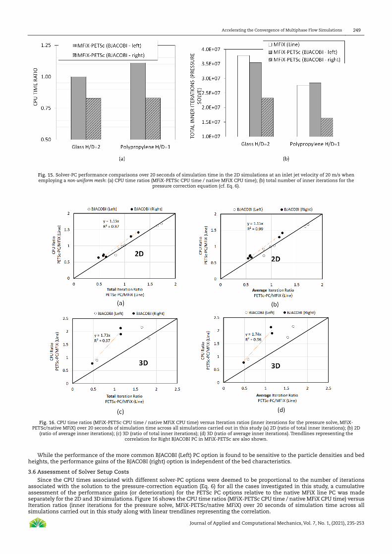
Fig. 15. Solver-PC performance comparisons over 20 seconds of simulation time in the 2D simulations at an inlet jet velocity of 20 m/s when employing a non-uniform mesh: (a) CPU time ratios (MFiX-PETSc CPU time / native MFiX CPU time); (b) total number of inner iterations for the

pressure correction equation (cf. Eq. 6).

Fig. 16. CPU time ratios (MFiX-PETSc CPU time / native MFiX CPU time) versus Iteration ratios (inner iterations for the pressure solve, MFiX-

PETSc/native MFiX) over 20 seconds of simulation time across all simulations carried out in this study (a) 2D (ratio of total inner iterations); (b) 2D (ratio of average inner iterations); (c) 3D (ratio of total inner iterations); (d) 3D (ratio of average inner iterations). Trendlines representing the

correlation for Right BJACOBI PC in MFiX-PETSc are also shown.

While the performance of the more common BJACOBI (Left) PC option is found to be sensitive to the particle densities and bed

heights, the performance gains of the BJACOBI (right) option is independent of the bed characteristics.

3.6 Assessment of Solver Setup Costs

Since the CPU times associated with different solver-PC options were deemed to be proportional to the number of iterations associated with the solution to the pressure-correction equation (Eq. 6) for all the cases investigated in this study, a cumulative assessment of the performance gains (or deterioration) for the PETSc PC options relative to the native MFiX line PC was made separately for the 2D and 3D simulations. Figure 16 shows the CPU time ratios (MFiX-PETSc CPU time / native MFiX CPU time) versus Iteration ratios (inner iterations for the pressure solve, MFiX-PETSc/native MFiX) over 20 seconds of simulation time across all simulations carried out in this study along with linear trendlines representing the correlation.



Fig. 17. Average and standard deviation of the number of solver iterations (inner iterations) for solving the pressure correction equation (cf. Eq. 8) in the fluidized bed simulations (H/D = 2) – A comparison of BJACOBI (Right) PC in PETSc with PFMG PC in HYPRE

First, we notice that the correlation is indeed linear for both 2D and 3D simulations. A slope of unity would indicate no overhead PETSc solver setup costs associated with solver object (h, �, and 0) creation and allocation. Figure 16 shows that this cost is minimal in the 2D simulations (Figure 16a, b) but non-negligible in the 3D simulations (Figure 16c, d). This means that in 3D simulations, the performance gains associated with a decrease in the number of iterations to achieve a specified solver tolerance should be greater than the overhead associated with the solver setup to result in a net decrease in CPU time associated with the simulation. As shown previously in Figure 14d, a simple reduction in the number of inner iterations in the 3D simulations (at the lower solver tolerance 1e-02) alone was not sufficient to result in a net decrease in CPU time (Figure 14a) compared to the native MFiX solver.

3.7 Multigrid (MG) Preconditioning

A preliminary integration of integrating the MFiX solve with the HYPRE linear solver library [35] was also carried out and the results are summarized in Figure 17.

The semi-coarsening multigrid PFMG was employed as a PC to the BiCGSTAB solver and converged to a tolerance of 1e-03. Results in Figure 17 show a significant reduction in the number of iterations to solve the pressure-correction equation in comparison to the MFiX-PETSc (BJACOBI – Right) option across all scenarios. The use of geometric MG option for multiphase flow scenarios is indeed very promising and billions of degrees of freedom can be tackled at large core counts [36]. However, a careful assessment of the set-up costs and performance degradation associated with MG solvers showed that these can be ameliorated as long as there is enough work to do per core as shown in [36, 37]. However, a rigorous validation of the numerical predictions followed by an assessment of solver set up costs in the HYPRE framework is ongoing and will be reported in a subsequent study. Nevertheless, this study has demonstrated the interfacing of the MFiX code with the PETSc and HYPRE linear solver libraries and has highlighted specific scenarios where the suite of solver-PC options in these numerical libraries may offer an advantage. With this framework in place, additional modifications can be undertaken to further accelerate the convergence of multiphase simulations. For instance, a recent study has shown that the SIMPLE method can be further accelerated (by a factor 3 - 5) when it is combined with a Krylov method [38] or that the variable coefficients in the Poisson equation that result in multiphase flow simulations can be avoided by employing fractional time-stepping techniques [39].

4. Conclusion

The need to accurately resolve near-wall phenomena and/or large L/D ratios associated with reactor configurations inevitably result in the generation of non-uniform grids characterized by: large aspect-ratios as well as variations in aspect ratios in various multiphase flow simulation scenarios. This, in conjunction with large density ratios of the constituent phases can further retard the convergence of the pressure-correction equation which constitutes a major bottleneck during the iterative solution to the to the incompressible Navier-Stokes equation. For single-phase flow problems, it has long been recognized that this shortcoming associated with the ill-conditioned pressure-correction matrix can be alleviated through appropriate pre-conditioning (PC) strategies to the iterative solver. This idea is extended in this study to multiphase simulation scenarios encompassing a wide range of fluidized bed scenarios.



We first interface the open-source multiphase simulation code MFiX with the PETSc linear solver library through an appropriate mapping of the matrix and vector data structures between the two software frameworks. Through this interface an access to a wide range of solver and PC options was then obtained. Among these, the Block Jacobi pre-conditioning to the BiCGTAB iterative solver was deemed to be the best PC-Solver option during the software verification process through timing studies performed on various test cases encompassing single-phase and multi-phase flow scenarios. In this paper, we compare the performance of this solver-PC combination against the default line-preconditioning option to BiCGSTAB in the native MFiX code for a class of bubbling bed simulations encompassing different: particle densities, bed-heights, inlet jet velocities, problem dimensions (2D/3D) and grid types (uniform/non-uniform). Taking a thin rectangular fluidized bed with a central jet as our reactor configuration (that has been experimentally investigated by other authors previously), the performances of various solver and PCs were compared on uniform grids as well as non-uniform grids that were well-resolved along the line near the central jet. Further, to ensure consistency when comparing PC performances, all of the solver-PC combinations were converged to the same residual tolerances. Our findings can be summarized as follows: 1. In all the simulations involving non-uniform grids with changes to the grid aspect ratios, the right-side Block Jacobi

preconditioning option in PETSc resulted in a 20 - 35% decrease in CPU time compared to the MFiX’s native solver-PC options when the linear solver tolerance was maintained at 1e-03. Further, the right-side Block Jacobi preconditioning performed better than the more commonly implemented left-side pre-conditioning option across all investigated scenarios.

2. The performance gains/losses achieved by the MFiX-PETSc interface over the native MFiX solver correlated well with a corresponding decrease in the number of iterations to reach a specified tolerance during the solution to the pressure-correction matrix equation. This confirmed that the solution to the pressure-correction equation was the computational bottleneck across all of the investigated scenarios.

3. When moving from uniform to non-uniform grids while the average number of solver iterations (to solve the pressure correction equation to a specified tolerance) increased across all PC options, this increase was greatest for MFiX’s line PC and the least with the BJACOBI (right) PC. This indicates that the BJACOBI (right) PC might perform more robustly when dealing with complex geometry and/or sudden changes to the grid sizes and aspect ratios.

4. While increasing the bed heights or the particle densities do increase: the average and total number of iterations for the pressure-correction equation and the number of time-steps to reach a given simulation time, the performance gains associated with the BJACOBI (right) PC option in the non-uniform grid simulations was found to be relatively independent of the bed material density or height.

5. The PETSc solver setup costs associated with solver object (E, F, and <) creation and allocation while being minimal in the 2D simulations was non-negligible in the 3D simulations. This means that in 3D simulations, the performance gains associated with a decrease in the number of iterations to achieve a specified solver tolerance should be greater than the overhead associated with the solver setup to result in a net decrease in CPU time associated with the simulation.

6. On uniformly spaced meshes however, MFiX’s native BiCGSTAB solver-line PC option performed better than the options in MFiX – PETSc both in terms of CPU times as well as in the number of iterations to reach a specified tolerance.

7. While the general fluidization characteristics were in reasonable agreement with experimental observations and identical between: the uniform and non-uniform grid simulations as well as between the different solver – PC options, the contours do not evolve in an identical manner among the different options as a result of the variable time-stepping algorithm employed in MFiX.

8. The choice of uniform/non-uniform grids or the solver-PC combination did not impact the time-averaged averaged pressure drop across the beds. In addition, the dynamic characteristics of the simulations were compared using power spectral density (PSD) plots of the pressure fluctuations over 10 seconds of simulation time. On log-log plots, the power-law decay of the PSD of pressure fluctuations across all simulations had slopes close to -4 in agreement with experimental observations. However, differences in solver-PC combinations sometimes resulted in differences in the identification of the dominant frequencies of the pressure fluctuations pointing towards a need to obtaining pressure samples over an extended period of time (> 10 seconds).

9. The time-step sizes resulting from MFiX’s automatic time-stepping algorithm were not significantly affected by the choice of the PC. This was ascertained by the fact that the total number of time-steps taken to reach a specified simulation time did not vary significantly among the various solver-PC combinations for each specific flow scenario.

Author Contributions

G. Krishnamoorthy planned and initiated the project and wrote the initial draft; L.E. Clarke helped develop the modeling framework, conducted the simulations, analyzed the results and assisted with the manuscript preparation; J.N. Thornock helped develop the modeling framework and conducted some of the simulations and assisted with the manuscript preparation. The manuscript was written through the contribution of all authors. All authors discussed the results, reviewed, and approved the final version of the manuscript.

Acknowledgments

We greatly appreciate discussions with Drs. Jordan Musser and Jean-Francois Dietiker (DOE-NETL).

Conflict of Interest

The authors declared no potential conflicts of interest with respect to the research, authorship, and publication of this article.

Funding

This research was funded through the University Coal Research Program being administered by DOE-NETL (Award #: DE-FE0026191).

Nomenclature

h Area of a control volume face, m2

E Matrix defining a linear system , Coefficients containing flow properties from discretized equations 0 Source term



< Right-hand side vector of a linear system ij Pressure coefficient i, k, , # Locations for TVD schemes b Diagonal matrix lm# Downwind factor for TVD schemes −C Lower triangular matrix −n Upper triangular matrix 3 Interface transfer coefficient # Fluid flow resistance due to porous media $ Acceleration due to gravity, m2/s Momentum transfer between two phases G Preconditioning matrix O Sparse lower triangular matrix for ILU � Pressure � Mass transfer of a chemical species due to reactions or other phenomena ℛ Mass transfer between two phases Q Residual matrix for ILU K Residual vector � Time, s Velocity component, m/s P Sparse upper triangular matrix for ILU o x-velocity component, m/s 2 Volume, m3 �, p, q Coordinate directions F Solution vector of a linear system Greek symbols � Volume fraction � Density, kg/m3 � Stress tensor r Relaxation factor for pressure correction equation > Relaxation parameter for the SOR preconditioner Ф General representation of a variable being solved Subscripts t Close packed regions u East control volume face comparative to v w East control volume central point comparative to � $ Fluid phase x, �, y Vector direction components � Solids phase 6 General phase number (fluid or solid) 60 Neighbor control volume faces or central points � Control volume central point at which a scalar variable is being solved v Control volume face at which velocity component is being solved m West control volume face comparative to v z West control volume central point comparative to � ∞ Inlet air stream conditions ′ Correction term for pressure or velocity ∗ Intermediate term for pressure or velocity } Normalized value

References

[1] Kunz, R.F., Boger, D.A., Stinebring, D.R., Chyczewski, T.S., Lindau, J.W., Gibeling, H.J., Venkateswaran, S., Govindan, T.R., A preconditioned Navier–Stokes method for two-phase flows with application to cavitation prediction, Computers & Fluids, 29(8), 2000, 849-875. [2] Syamlal, M., MFIX documentation: numerical technique, National Energy Technology Laboratory, Department of Energy, Technical Note No. DOE/MC31346-5824, 1998. [3] Hua, J., Lou, J., Numerical simulation of bubble rising in viscous liquid, Journal of Computational Physics, 222, 2007, 769-795. [4] Duffy, A.U., Kuhnle, A.L., Sussman, M., An improved variable density pressure projection solver for adaptive meshes, From URL https://www.math.fsu.edu/~sussman/MGAMR.pdf (last accessed: 4/26/2018) [5] Dehbi, A., A CFD model for particle dispersion in turbulent boundary layer flows, Nuclear Engineering and Design, 238(3), 2008, 707-715. [6] Saito, Y., Takami, R., Nakamori, I., Ikohagi, T., Numerical analysis of unsteady behavior of cloud cavitation around a NACA0015 foil, Computational Mechanics, 40(1), 2007, 85. [7] Gupta, R., Fletcher, D.F., Haynes, B.S., CFD modelling of flow and heat transfer in the Taylor flow regime, Chemical Engineering Science, 65(6), 2010, 2094-2107. [8] Ryan, E.M., DeCroix, D., Breault, R., Xu, W., Huckaby, E.D., Saha, K., Dartevelle, S., Sun, X. , Multi-phase CFD modeling of solid sorbent carbon capture system, Powder Technology, 242, 2013, 117-134. [9] Tingwen Li, A.G., Pannala, S., Shahnama, M., Syamlal, M., CFD simulations of circulating fluidized bed risers, part II, evaluation of differences between 2D and 3D simulations, Powder Technology, 265, 2014, 13-22. [10] Ghadirian, M., Hayes, R.E., Mmbaga, J., Afacan, A., Xu, Z., On the simulation of hydrocyclones using CFD, The Canadian Journal of Chemical Engineering, 91(5), 2013, 950-958. [11] Li, T., Dietiker, J.F., Zhang, Y., Shahnam, M., Cartesian grid simulations of bubbling fluidized beds with a horizontal tube bundle, Chemical Engineering Science, 66(23), 2011, 6220-6231. [12] Coutier-Delgosha, O., Fortes-Patella, R., Reboud, J.L., Hofmann, M., Stoffel, B., Experimental and numerical studies in a centrifugal pump with two-dimensional curved blades in cavitating condition, Journal of Fluids Engineering, 125(6), 2003, 970-978. [13] Smith, J., Matrix Solution Techniques for CFD Applications on Non-Uniform Grids, In ASME 2004 Heat Transfer/Fluids Engineering Summer Conference, pp. 1319-1324, American Society of Mechanical Engineers, 2004. [14] Buelow, P.E.O., Venkateswaran, S., Merkle, C.L., Effect of grid aspect ratio on convergence, AIAA Journal, 32(12), 1994, 2401-2408. [15] Hu, Y.F., Carter, J.G., Blake, R.J., The effect of the grid aspect ratio on the convergence of parallel CFD algorithms, Parallel Computational Fluid Dynamics,



1995, 289-296. [16] Coutier-Delgosha, O., Fortes-Patella, R., Reboud, J.L., Hakimi, N., Hirsch, C., Stability of preconditioned Navier–Stokes equations associat,ed with a cavitation model, Computers & Fluids, 34(3), 2005, 319-349. [17] Syamlal, M., Rogers, W., O’Brien, T.J., MFIX documentation: theory guide, U.S. Dept. of Energy, Office of Fossil Energy, Technical Note No. DOE/METC-94/1004, 1993. [18] Balay, S., Abhyankar, S., Adams, M., Brown, J., Brune, P., Buschelman, K., Dalcin, L., Eijkhout, V., Gropp, W., Karpeyev, D., Kaushik, D., Knepley, M., May, D., McInnes, L.C., Mills, R., Munson, T., Rupp, K., Sanan, P., Smith, B., Zampini, S., Zhang, H., Zhang, H., PETSc users manual, Argonne National Laboratory, ANL-95/11 Rev. 3.9, 2013. [19] Zhang, J., Preconditioned Krylov subspace methods for solving nonsymmetric matrices from CFD applications, Computer Methods in Applied Mechanics and Engineering, 189(3), 2000, 825-840. [20] Ghai, A., Lu, C., Jiao, X., A comparison of preconditioned krylov subspace methods for large-scale nonsymmetric linear systems, arXiv:1607.00351, 2017. [21] Musser, J., Choudhary, A., MFIX documentation volume 3: verification and validation manual, National Energy Technology Laboratory, From URL https://mfix.netl.doe.gov/download/mfix/mfix_current_documentation/MDV3-VVUQ-v0.5.pdf, 2015 (last accessed: 6/24/2018). [22] Syamlal, M., Musser, J., Dietiker, J.F., The two-fluid model in MFIX, In: Multiphase Flow Handbook (2nd Ed.), Boca Rotan, FL, USA, Taylor & Francis Group, LLC, 242-275, 2017. [23] Patankar, S.V., Numerical heat transfer and fluid flow, New York, Hemisphere Publishing Corporation, 1980. [24] Clarke, L.E., Interfacing the CFD Code MFiX with the PETSc Linear Solver Library to Achieve Reduced Computation Times, MS Thesis, The University of North Dakota, 2018 [25] Saad, Y., Iterative Methods for Sparse Linear Systems, 2nd ed., Society for Industrial and Applied Mathematics, 2013. [26] Hiroto, T., Sakurai, T., On single precision preconditioners for Krylov subspace iterative methods, In International Conference on Large-Scale Scientific Computing, pp. 721-728. Springer, Berlin, Heidelberg, 2007. [27] Leonard, B.P., Mohktari, S., Beyond first-order upwinding: the ultra-sharp alternative for non-oscillatory steady-state simulation of convection, International Journal for Numerical Methods in Engineering, 30(4), 1990, 729-766. [28] Wang, Z.J., Fidkowski, K., Abgrall, R., Bassi, F., Caraeni, D., Cary, A., Deconinck, H., Harmann, R., Hillewaert, K., Huynh, H.T., Kroll, N., May, G., Persson, P.-O., van Leer, B., Visbal, M., High‐order CFD methods: current status and perspective, International Journal for Numerical Methods in Fluids, 72(8), 2013, 811-845. [29] Utikar, R.P., Ranade, V.V., Single jet fluidized beds: experiments and CFD simulations with glass and polypropylene particles, Chemical Engineering Science, 62(1-2), 2007, 167-183. [30] Uddin, M.H., Coronella, C.J., Effects of grid size on predictions of bed expansion in bubbling fluidized beds of Geldart B particles: A generalized rule for a grid-independent solution of TFM simulations, Particuology, 34, 2017, 61-69. [31] Dietiker, J.-F., MFIX results sensitivity to Fortran compilers. From URL https://mfix.netl.doe.gov/download/mfix/mfix_current_documentation/MFIX_results_sensitivity_to_Fortran_compilers.pdf (2012) (last accessed: 7/24/2018) [32] Van Wachem, B.G.M., Schouten, J.C., Krishna, R., Van den Bleek, C.M., Validation of the Eulerian simulated dynamic behaviour of gas–solid fluidised beds, Chemical Engineering Science, 54(13-14), 1999, 2141-2149. [33] Hernández-Jiménez, F., Sánchez-Delgado, S., Gómez-García, A., Acosta-Iborra, A., Comparison between two-fluid model simulations and particle image analysis & velocimetry (PIV) results for a two-dimensional gas–solid fluidized bed, Chemical Engineering Science, 66(17), 2011, 3753-3772. [34] Benyahia, S., Fine‐grid simulations of gas‐solids flow in a circulating fluidized bed, AIChE Journal, 58(11), 2012, 3589-3592. [35] Chow, E., Cleary, A.J., Falgout, R.D., Design of the Hypre Preconditioner Library, Lawrence Livermore National Laboratory, UCRL-JC-132025, Livermore, California, 1998 [36] Kronbichler, M., Diagne, A., Holmgren, H., A fast massively parallel two-phase flow solver for microfluidic chip simulation, The International Journal of High Performance Computing Applications, 32(2), 2018, 266-287. [37] Schmidt, J., Berzins, M., Thornock, J., Saad, T., Sutherland, J.C., Large scale parallel solution of incompressible flow problems using uintah and hypre, In Cluster, Cloud and Grid Computing (CCGrid), 13th IEEE/ACM International Symposium, pp. 458-465, 2013. [38] Klaij, C.M., Vuik, C., SIMPLE‐type preconditioners for cell‐centered, colocated finite volume discretization of incompressible Reynolds‐averaged Navier–Stokes equations, International Journal for Numerical Methods in Fluids, 71(7), 2013, 830-849. [39] Guermond, J.L., Salgado, A., A splitting method for incompressible flows with variable density based on a pressure Poisson equation, Journal of Computational Physics, 228(8), 2009, 2834-2846.

ORCID iD

Gautham Krishnamoorthy https://orcid.org/0000-0002-5520-5092 Lauren Elizabeth Clarke https://orcid.org/ 0000-0003-4780-2791 Jeremy Nicholas Thornock https://orcid.org/0000-0002-6587-9437

© 2020 by the authors. Licensee SCU, Ahvaz, Iran. This article is an open access article distributed under the terms and conditions of the Creative Commons Attribution-NonCommercial 4.0 International (CC BY-NC 4.0 license) (http://creativecommons.org/licenses/by-nc/4.0/).

How to cite this article: Krishnamoorthy G., Clarke L.E., Thornock, J.N.. Accelerating the Convergence of Multiphase Flow Simulations when Employing Non-Uniform Structured Grids, J. Appl. Comput. Mech., 7(1), 2021, 235–253. https://doi.org/10.22055/JACM.2020.35096.2563

accelerating the convergence of multiphase flow

Documents