abstracts - hgg.au.dkhgg.au.dk/fileadmin/ · reff =8fk. (2) a good estimation of reff is a decisive...
TRANSCRIPT

Abstracts from session A
IP2016 – 6-8 June, Aarhus, Denmark 1
Induced polarization and pore radius – a discussion Andreas Weller Zeyu Zhang Lee Slater Institut für Geophysik, TU Clausthal Southwest Petroleum University Rutgers University Arnold-Sommerfeld-Str.1, Institute of Earth Science and Technology Dpt. Earth and Environm. Sci. 38678 Clausthal-Zellerfeld, Germany Chengdu, China Newark, New Jersey, USA [email protected] [email protected] [email protected] Sabine Kruschwitz Matthias Halisch Bundesanstalt für Materialforschung und –prüfung Leibniz-Institut für Angewandte Geophysik Unter den Eichen 87, 12205 Berlin, Germany Stilleweg 1, 30655 Hannover, Germany [email protected] [email protected]
INTRODUCTION
The key parameters for reservoir characterization are porosity and permeability. A variety of field, logging and laboratory methods provide porosity. Permeability can be determined by gas flow measurements in the lab. Permeability prediction in a field or logging survey is based on correlations to other measurable parameters. Beside porosity, the pore size is an important parameter that is closely related to permeability. However, the determination of a reliable value of an effective pore size is a challenging problem. The Mercury Intrusion Capillary Pressure method (MICP) provides the distribution of the pore throat radius. Nuclear Magnetic Resonance (NMR) is
another useful method that can be used to estimate the pore size distribution. MICP is a laboratory method. Under favourable conditions, NMR is also applicable in field surveys. Induced Polarization (IP) has been proposed to be another potential method providing access to the pore size distribution. Several authors observed relations between the pore size and different types of relaxation times (e.g. Scott and Barker, 2003; Binley et al., 2005; Kruschwitz et al. 2010). It is difficult to explain all these observations by a uniform physical model. Instead of a pore size distribution, a so-called characteristic pore size is assumed. Most authors prefer to use the dominant pore size determined from MICP that corresponds to the pressure of maximal incremental mercury intrusion. Similarly, a characteristic relaxation time is assumed, which can be determined by different procedures. The resulting time constant from fitting procedures related to models of the Cole-Cole type is a widely used approach. Others use the mean relaxation time resulting from Debye decomposition (Nordsiek and Weller, 2008). In other approaches, if the measured IP spectra show a maximum in the curves of imaginary part of conductivity or the phase angle the frequency of the maximum is simply transformed into a relaxation time (Scott and Barker, 2003; Revil et al., 2015). The latter approach is quite simple because it does not require any fitting procedure. We used this approach for a set of sandstone samples that has been investigated in different labs. All IP spectra show a maximum of imaginary part of conductivity inside the investigated frequency interval between 2 mHz and 100 Hz. The effective hydraulic radius of this set of samples has been determined from permeability and formation factor. We evaluate whether any relation between characteristic relaxation time and effective hydraulic radius exists.
METHOD The simplest model of permeability prediction is based on bundles of uniform capillaries that pervade a solid medium. Based on geometric considerations and considering the Hagen-Poiseuille equation, permeability k can be easily determined by the geometric quantities porosity φ, pore radius r and tortuosity T according to the following equation:
.8
2
T
rk
φ= (1)
The ratio T/φ can be replaced by the formation factor if the electric tortuosity is assumed to equal the hydraulic tortuosity. Equation 1 can be used to determine an effective hydraulic
SUMMARY Permeability estimation from spectral induced polarization (SIP) measurements is based on a fundamental premise that the characteristic relaxation time (τ) is related to the effective hydraulic radius (reff) controlling fluid flow. The approach requires a reliable estimate of the diffusion coefficient of the ions in the electrical double layer. Others have assumed a value for the diffusion coefficient, or postulated different values for clay versus clay-free rocks. We examine the link between τ and reff for an extensive database of sandstone samples where mercury porosimetry data confirm that reff is reliably determined from a modification of the Hagen-Poiseuille equation assuming that the electrical tortuosity is equal to the hydraulic tortuosity. Our database does not support the existence of 1 or 2 distinct representative diffusion coefficients but instead demonstrates strong evidence for 6 orders of magnitude of variation in an apparent diffusion coefficient that is well correlated with both reff and the specific surface area per unit pore volume (Spor). Two scenarios can explain our findings: (1) the length-scale defined by τ is not equal to reff and is likely much longer due to the control of pore surface roughness; (2) the range of diffusion coefficients is large and likely determined by the relative proportions of the different minerals (e.g. silica, clays) making up the rock. In either case, the estimation of reff (and hence permeability) is inherently uncertain from SIP relaxation time. Key words: pore radius, mercury intrusion capillary pressure, spectral induced polarization, relaxation time.
Induced polarization and pore radius Weller et al.
IP2016 – 6-8 June, Aarhus, Denmark 2
radius reff of any sample if permeability and formation factor are known:
Fkreff 8= . (2)
A good estimation of reff is a decisive step in permeability prediction because the variation in the formation factor is considerably lower than in reff. A variety of models have recently been proposed to relate a characteristic pore size Λ with a characteristic relaxation time τ0 (Revil et al., 2012; 2015):
)(
2
0 2 +
Λ=D
τ (3)
with D(+) being the diffusion coefficient of the ions in the Stern layer. A characteristic relaxation time τpeak can easily be determined from the frequency of the maximum (peak frequency fpeak) of the spectrum of imaginary part of conductivity σ”( f):
peak
peak fπτ
2
1= (4)
assuming that a measurable maximum exists inside the investigated frequency range. We equate the effective hydraulic radius reff that is determined from equation 2 to the characteristic pore size Λ. The resulting equation
peakeff Dr τ)(2 += (5)
relates the relaxation time τpeak to the effective hydraulic radius reff. We check the general validity of equation 5 for a set of sandstone samples.
SAMPLES Our set of sandstone samples originates from several studies including 21 Eocene sandstone samples of the Shahejie formation (CS samples, China, Zhang and Weller, 2014), eight samples of the Cretaceous Bahariya formation (Egypt), and 17 samples from different locations in Germany (Bentheimer, Buntsandstone, Elbe-sandstone, Flechtinger, Green sand, Obernkirchen, Röttbacher, Udelfanger), France (Fontainebleau), Poland (Skala), the UK (Helsby), and Vietnam (Dong Do). All samples are characterized by a measurable maximum in the spectrum of the imaginary part of conductivity. The permeability and the formation factor of all samples are known and the effective hydraulic radius reff has been determined by equation 2. Additionally, MICP measurements and the specific surface area per unit volume (Spor) of most samples are available.
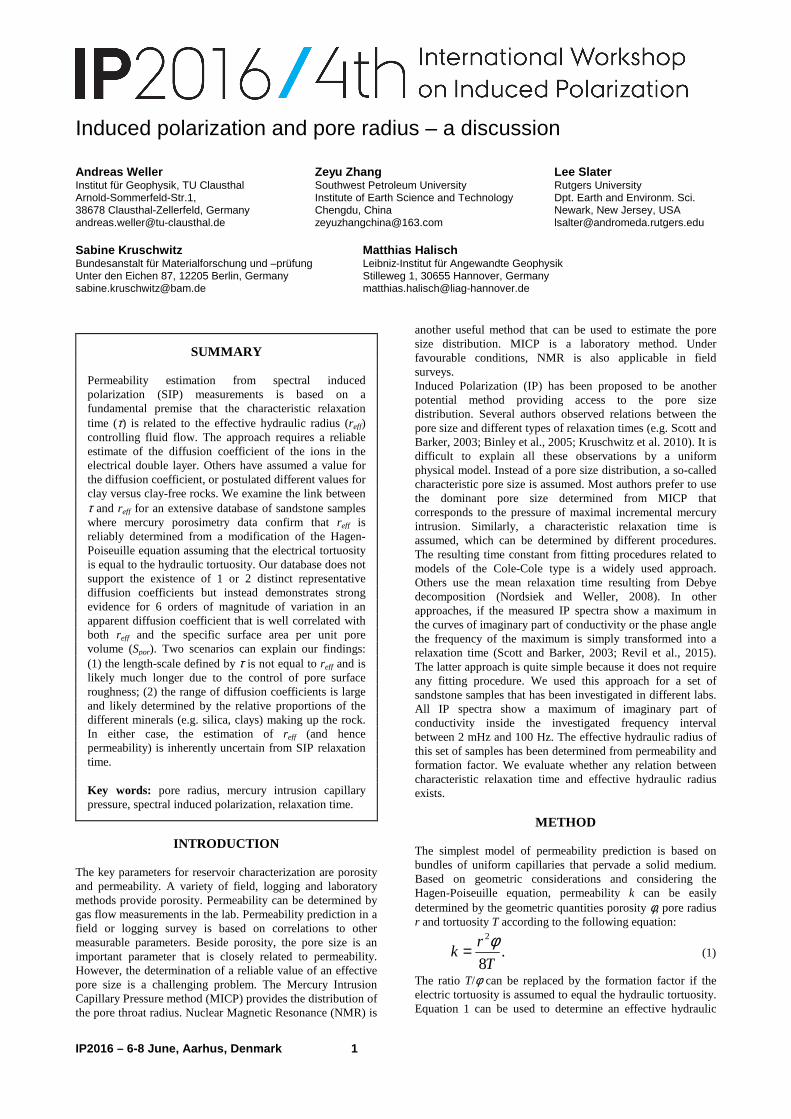
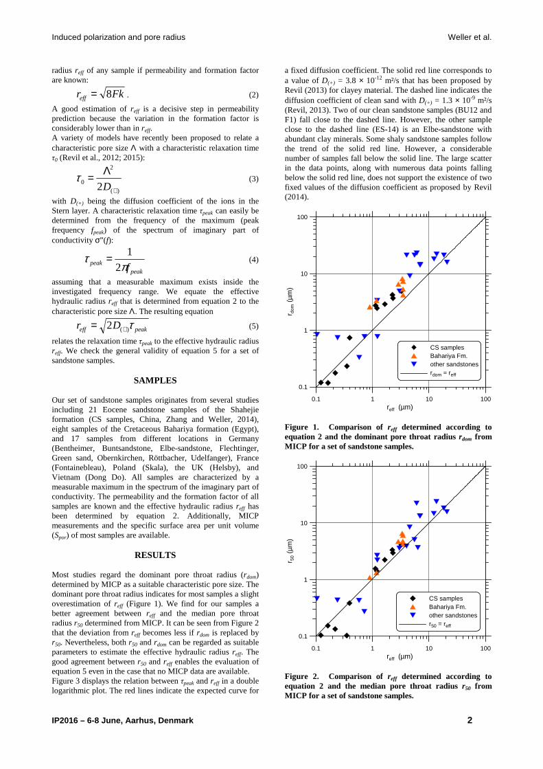
RESULTS Most studies regard the dominant pore throat radius (rdom) determined by MICP as a suitable characteristic pore size. The dominant pore throat radius indicates for most samples a slight overestimation of reff (Figure 1). We find for our samples a better agreement between reff and the median pore throat radius r50 determined from MICP. It can be seen from Figure 2 that the deviation from reff becomes less if rdom is replaced by r50. Nevertheless, both r50 and rdom can be regarded as suitable parameters to estimate the effective hydraulic radius reff. The good agreement between r50 and reff enables the evaluation of equation 5 even in the case that no MICP data are available. Figure 3 displays the relation between τpeak and reff in a double logarithmic plot. The red lines indicate the expected curve for
a fixed diffusion coefficient. The solid red line corresponds to a value of D(+) = 3.8 × 10⁻¹² m²/s that has been proposed by Revil (2013) for clayey material. The dashed line indicates the diffusion coefficient of clean sand with D(+) = 1.3 × 10⁻⁹ m²/s (Revil, 2013). Two of our clean sandstone samples (BU12 and F1) fall close to the dashed line. However, the other sample close to the dashed line (ES-14) is an Elbe-sandstone with abundant clay minerals. Some shaly sandstone samples follow the trend of the solid red line. However, a considerable number of samples fall below the solid line. The large scatter in the data points, along with numerous data points falling below the solid red line, does not support the existence of two fixed values of the diffusion coefficient as proposed by Revil (2014).
0.1 1 10 100reff (µm)
0.1
1
10
100
r dom
(µm
)
CS samplesBahariya Fm.other sandstonesrdom = reff
Figure 1. Comparison of reff determined according to equation 2 and the dominant pore throat radius rdom from MICP for a set of sandstone samples.
0.1 1 10 100reff (µm)
0.1
1
10
100
r 50
(µm
)
CS samplesBahariya Fm.other sandstonesr50 = reff
Figure 2. Comparison of reff determined according to equation 2 and the median pore throat radius r50 from MICP for a set of sandstone samples.

Induced polarization and pore radius Weller et al.
IP2016 – 6-8 June, Aarhus, Denmark 3
-2.5 -2 -1.5 -1 -0.5 0 0.5 1log(τpeak in s)
-1
-0.5
0
0.5
1
1.5
log(
r eff
in µ
m)
Bu-1
ES-14
GR-1
OK-4
BH7
BR5
BU3
BU12
GR1F1
NS2/2R
Roett
Ska
Ud
BE
FL
OK
CS samplesBahariyaother sandstonesD(+) = 3.8 µm²/s
D(+) = 1300 µm²/s
Figure 3. Comparison between τpeak and reff in a double logarithmic plot for a set of sandstone samples.
0.1 1 10 100reff (µm)
0.01
0.1
1
10
100
1000
Da
(µm
2 /s)
CS samplesBahariyaother sandstonesDa = 0.782 (reff)1.77
Da = 3.8 µm²/s
Da = 1300 µm²/s
Figure 4. Relation between effective hydraulic radius reff and apparent diffusion coefficient Da for a set of sandstone samples. Assuming the validity of equation 5, an apparent diffusion coefficient Da can be defined:
peak
effa
rD
τ2
2
= . (6)
This apparent diffusion coefficient, which can be determined for each sample, is presented as a function of reff in Figure 4. It varies over a range of nearly six orders of magnitude. A remarkable trend is observed: the increasing effective hydraulic radius is accompanied by an increasing apparent diffusion coefficient. The fitting equation reads
77.1782.0 effa rD = . (7)
with Da given in µm2/s and reff. in µm. Kruschwitz et al. (2010) reported a similar trend for their set of sandstone samples. They determined an apparent diffusion coefficient from the dominant pore throat diameter ddom and the time constant of a generalized Cole-Cole fitting model. The resulting graph indicates the proportionality
68.1
doma dD ∝ (8)
with a similar exponent. Figure 5 displays the relation between the specific surface area per unit pore volume Spor and the apparent diffusion coefficient Da. An increasing specific internal surface is related to a decrease in Da.
0.1 1 10 100 1000Spor (1/µm)
0.01
0.1
1
10
100
1000
Da
(µm
2 /s)
CS samplesBahariyaother sandstonesDa = 49.4 (Spor)-1.31
Figure 5. Relation between specific surface area Spor and apparent diffusion coefficient Da for a set of sandstone samples.
DISSCUSSION The wide variation in apparent diffusion coefficient and its dependence on effective hydraulic radius and the specific surface area raises doubt regarding the applicability of equation 5 for estimating pore geometric characteristics of sandstone samples. There are two main concerns: (1) The effective hydraulic radius cannot be the relevant pore size for IP relaxation if a nearly constant diffusion coefficient is assumed for the clayey sandstone samples. The diffusion path would be considerably longer than the pore radius for most samples that are displayed below the solid red line in Figure 3. The increasing pore surface roughness, which is reflected by larger values of Spor, generates a considerable surface tortuosity and longer diffusion paths along the pore surface. It can be assumed that the true length of the diffusion path can be determined by IP relaxation time, but this length is not simply related to the effective hydraulic radius. (2) A decrease in the ion mobility and consequently in the diffusion coefficient caused by increasing clay content and increasing specific surface area offers an alternative explanation of the experimental findings. It can be expected that a stronger binding of ions at the surfaces of clay minerals

Induced polarization and pore radius Weller et al.
IP2016 – 6-8 June, Aarhus, Denmark 4
dominates the diffusion in smaller pores. A variation of the diffusion coefficient with the type and amount of clay makes the application of equation 5 for estimating reff difficult. A permeability prediction that assumes the validity of equation 5 and a constant diffusion coefficient will only work for those samples that are indicated close to the red lines in Figure 3. In the specific case of the plotted red lines, the apparent diffusion coefficient is close to the assumed diffusion coefficient for either clayey material (solid line) or clean sandstones (dashed line). The majority of samples indicates a diffusion coefficient different from these two fixed values. Most samples with an apparent diffusion coefficient lower than the value of clayey material (D(+) = 3.8 × 10⁻¹² m²/s) are characterized by an effective pore radius smaller than 2 µm and a permeability smaller than 1 mD. Revil et al. (2015) exclude these samples from their approach of permeability prediction based on IP relaxation time and formation factor. The binary binning into clayey material and clean sands has been recently disputed (Revil, 2014; Weller et al., 2014). Our experimental findings do not support the existence of two fixed values of the diffusion coefficient. Considering the varying clay content in our samples, it would be difficult to define a sharp boundary between the two groups. What concentration of clay minerals would be tolerated in a sandstone for it to be referred to as clean sand? In our opinion, a sandstone should be characterized by an effective diffusion coefficient representing a weighting between the different minerals. The data points falling between the two red lines in Figure 3 indicate the existence of sandstone samples with behaviour between clean sand and clayey material. All approaches of permeability prediction that are based on IP relaxation time remain problematic. Sandstone samples that do not indicate a characteristic relaxation time in the investigated frequency cannot be considered. As shown in our study, the relation between IP relaxation time and pore size is far from unique. Alternative approaches, which are based on quadrature conductivity instead of relaxation time, have proved to be successful in permeability prediction of sandstones and unconsolidated material (e.g. Weller et al., 2015).
CONCLUSIONS Our study presents experimental evidence that the effective hydraulic radius, which is a key parameter in permeability prediction, cannot be determined by the IP relaxation time in a direct way. The apparent diffusion coefficient that relates effective hydraulic radius and IP relaxation time varies over six orders of magnitude. The assumption of a constant diffusion coefficient suggests that the true diffusion path is much larger than the effective hydraulic radius. A strongly varying diffusion coefficient has to be assumed if the effective hydraulic radius is accepted to be related to the diffusion length. The practical use of IP relaxation time is strongly restricted if both effective hydraulic radius and diffusion coefficient are variable parameters in sandstone samples.
ACKNOWLEDGMENTS The authors thank Katrin Breede, Henning Schröder, and Nguyen Trong Vu for providing data of their sandstone samples.
REFERENCES Binley, A., Slater, L. D., M. Fukes, M., and Cassiani, G., 2005, Relationship between spectral induced polarization and hydraulic properties of saturated and unsaturated sandstone, Water Resources Research., 41, W12417, doi:10.1029/2005WR004202. Kruschwitz, S. F., Binley, A., Lesmes, D., and A. Elshenawy, A., 2010, Textural controls on low-frequency electrical spectra of porous media: Geophysics, 75, 4, WA113–WA123. Nordsiek, S., and Weller, A., 2008, A new approach to fitting induced-polarization spectra: Geophysics, 73, No. 6, F235-F245, doi: 10.1190/1.2987412. Revil, A., 2013, Effective conductivity and permittivity of unsaturated porous materials in the frequency range 1 mHz-1GHz, Water Resources Research, 49, 306-327, doi: 10.1029/2012WR012700. Revil, A., 2014, Comment on: “On the relationship between induced polarization and surface conductivity: Implications for petrophysical interpretation of electrical measurements” (A. Weller, L. Slater, and S. Nordsiek, Geophysics, 78, no. 5, D315-D325): Geophysics, 79, no. 2, X1-X5. Revil, A., Binley, A., Mejus, L., and Kessouri, P., 2015, Predicting permeability from characteristic relaxation time and intrinsic formation factor of complex conductivity spectra: Water Resources Research, 51, 6672-6700, doi:10.1002/2015WR017074. Revil, A., Koch, K., and Holliger, K., 2012, Is it the grain size or the characteristic pore size that controls the induced polarization relaxation time of clean sands and sandstones?, Water Resources Research, 48, W05602, doi:10.1029/2011WR011561. Scott, J. B., and Barker, R., 2003, Determining pore-throat size in Permo-Triassic sandstones from low-frequency electrical spectroscopy: Geophysical Research Letters, 30(9), 1450, doi:10.1029/2003GL016951. Weller, A., Slater, L., and Nordsiek, S., 2014, Reply to the discussion by A. Revil, Comment on: “On the relationship between induced polarization and surface conductivity: Implications for petrophysical interpretation of electrical measurements” (A. Weller, L. Slater, and S. Nordsiek, Geophysics, 78, no. 5, D315-D325): Geophysics, 79, no. 2, X6-X10. Weller, A., Slater, L., Binley, A., Nordsiek, S., and Xu, S., 2015, Permeability prediction based on induced polarization: Insights from measurements on sandstone and unconsolidated samples spanning a wide permeability range: Geophysics 80, No. 2, D161-D173. Zhang, Z., and Weller, A., 2014, Fractal dimension of pore-space geometry of an Eocene sandstone formation: Geophysics, 79, No. 6, D377-D387. doi: 10.1190/geo2014-0143.1.

IP2016 – 6-8 June, Aarhus, Denmark 1
Modeling the evolution of spectral induced polarization during calcite precipitation on glass beads Leroy Philippe Li Shuai Jougnot Damien Revil André Wu Yuxin BRGM Imperial College CNRS, UMR 7619 METIS CNRS, UMR 5275 LBNL
Orléans, France London, England Paris, France Le Bourget du Lac, France Berkeley, USA.
[email protected] [email protected] [email protected] [email protected] [email protected]
INTRODUCTION
Calcite is one of the most abundant minerals in the earth crust
and frequently precipitates when alkalinity and pH increase
(Vancappellen et al., 1993). Calcite precipitation modifies the
rock porosity, and can have positive or harmful effects for the
mechanical and transport properties of porous media. Calcite
precipitation in porous media has broad applications in
geotechnical engineering for soil strengthening (DeJong et al.,
2006) and in environmental studies for the sequestration of
heavy metals (Sturchio et al., 1997), radionuclides (Fujita et
al., 2004) and CO2 in geological formations (Pruess et al.,
2003). However, calcite precipitation can also have undesirable
effects such as the decrease of the efficiency and permeability
of reactive barriers for the remediation of aquifers (Wilkin et
al., 2003).
Wu et al. (2010) performed complex conductivity
measurements and modeling of calcite precipitation on glass
beads packed column. From their imaginary part of complex
conductivity data, the evolution of calcite precipitation in
porous media was clearly observed. The empirical Cole-Cole
model (Cole and Cole, 1941) was used by Wu et al. (2010) to
interpret the complex conductivity signature of calcite
precipitation in glass beads. However, the lack of physical
processes in the Cole-Cole model to interpret the complex
conductivity data restricts the understanding of the effects of
calcite precipitation on the evolution of the pore structure and
connectivity in glass beads column. The induced polarization
of calcite precipitates needs to be further clarified using a
mechanistic complex conductivity model accounting for the
EDL properties and the particle size distribution. In this study,
a mechanistic model for the induced polarization of calcite is
proposed, which depends on the surface charge density and
ions mobility of the counter-ions in the Stern layer and on the
particle size distribution. The predictions of the model are
compared to the imaginary conductivity data of Wu et al.
(2010), and the evolution of the pore structure during calcite
precipitation in glass beads is estimated accordingly.
THEORETICAL BACKGROUND AND
COMPARISON WITH EXPERIMENTAL DATA
We consider a porous medium containing particles, glass
beads grains (of millimetric size) and calcite crystals (of
micrometric size), and water (subscript “w”). The complex
conductivity model is presented at Figure 1.
Figure 1. Sketch of thecomplex conductivity model of the
porous medium.
Maxwell-Wagner polarization occurs at the boundary between
the different phases (solid, water) possessing different
electrical properties. The differential effective medium (DEM)
theory (Sen et al., 1981) is used to compute the electrical
conductivity of the porous medium according to the
conductivity of the particles and liquid. The complex surface
SUMMARY
When pH and alkalinity increase, calcite frequently
precipitates and hence modifies the petrophysical
properties of porous media. The complex conductivity
method can be used to directly monitor calcite
precipitation in porous media because it is very sensitive
to the evolution of the pore structure and its connectivity.
We have developed a mechanistic grain polarization
model considering the electrochemical polarization of the
Stern layer surrounding calcite particles. This model
depends on the surface charge density and mobility of the
counter-ions in the Stern layer. Our induced polarization
model predicts the evolution of the size of calcite
particles, of the pore structure and connectivity during
spectral induced polarization experiments of calcite
precipitation on glass beads pack. Model predictions are
in very good agreement with the complex conductivity
measurements. During the first phase of calcite
precipitation experiment, calcite crystals growth, and the
inverted particle size distribution moves towards larger
calcite particles. When calcite continues to precipitate and
during pore clogging, inverted particle size distribution
moves towards smaller particles because large particles do
not polarize sufficiently. The pore clogging is also
responsible for the decrease of the connectivity of the
pores, which is observed through the increasing electrical
formation factor of the porous medium.
Key words: calcite precipitation, complex conductivity,
Stern layer, particle size, pore clogging.
Modeling spectral induced polarization of calcite precipitation Leroy, P., Li, S., Jougnot, D., Revil, A., Wu, Y. eg: Author1, Author2 and Author3
IP2016 – 6-8 June, Aarhus, Denmark 2
conductivity of the particles of different sizes is calculated
considering the superposition principle and using the particle
size distribution (PSD) (Leroy et al., 2008). The complex
surface conductivity of the particle is computed using the
spectral induced polarization model of Leroy et al. (2008)
generalized to the electrochemical polarization of different
counter-ions at the mineral/water interface. The specific
surface conductivity of the particle is calculated considering
the superposition of the AC (Stern layer) and DC current
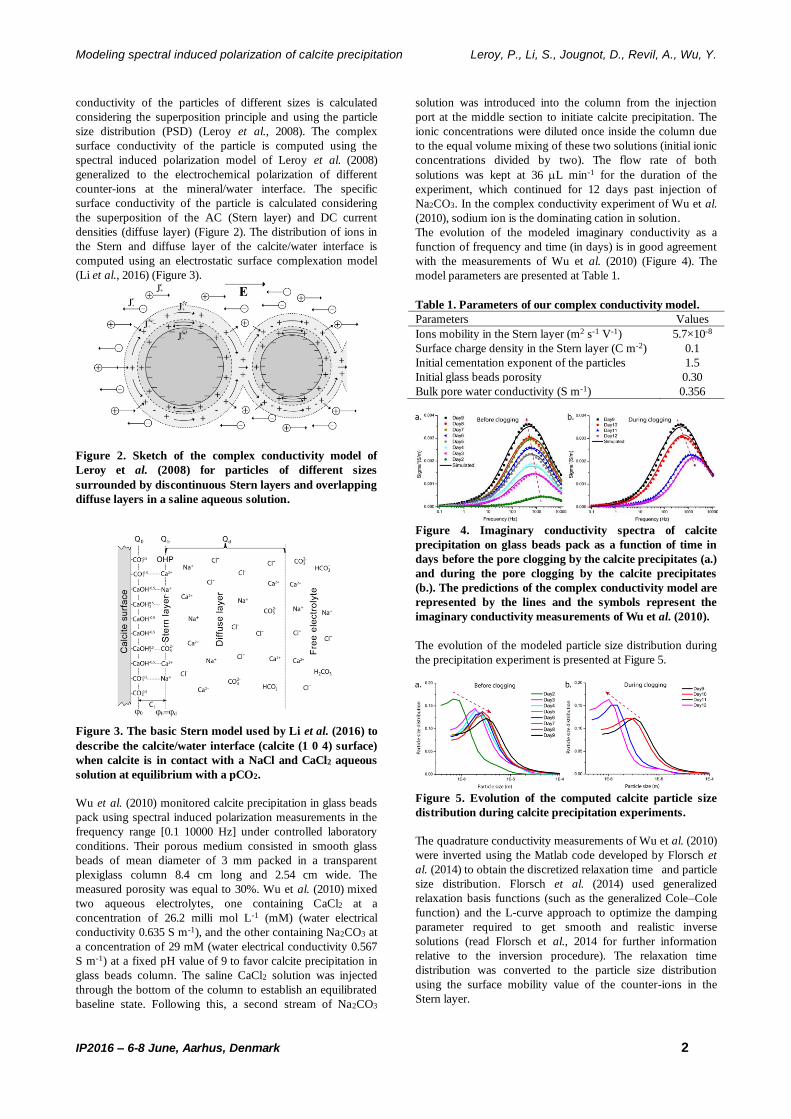
densities (diffuse layer) (Figure 2). The distribution of ions in
the Stern and diffuse layer of the calcite/water interface is
computed using an electrostatic surface complexation model
(Li et al., 2016) (Figure 3).
Figure 2. Sketch of the complex conductivity model of
Leroy et al. (2008) for particles of different sizes
surrounded by discontinuous Stern layers and overlapping
diffuse layers in a saline aqueous solution.
Figure 3. The basic Stern model used by Li et al. (2016) to
describe the calcite/water interface (calcite (1 0 4) surface)
when calcite is in contact with a NaCl and CaCl2 aqueous
solution at equilibrium with a pCO2.
Wu et al. (2010) monitored calcite precipitation in glass beads
pack using spectral induced polarization measurements in the
frequency range [0.1 10000 Hz] under controlled laboratory
conditions. Their porous medium consisted in smooth glass
beads of mean diameter of 3 mm packed in a transparent
plexiglass column 8.4 cm long and 2.54 cm wide. The
measured porosity was equal to 30%. Wu et al. (2010) mixed
two aqueous electrolytes, one containing CaCl2 at a
concentration of 26.2 milli mol L-1 (mM) (water electrical
conductivity 0.635 S m-1), and the other containing Na2CO3 at
a concentration of 29 mM (water electrical conductivity 0.567
S m-1) at a fixed pH value of 9 to favor calcite precipitation in
glass beads column. The saline CaCl2 solution was injected
through the bottom of the column to establish an equilibrated
baseline state. Following this, a second stream of Na2CO3
solution was introduced into the column from the injection
port at the middle section to initiate calcite precipitation. The
ionic concentrations were diluted once inside the column due
to the equal volume mixing of these two solutions (initial ionic
concentrations divided by two). The flow rate of both
solutions was kept at 36 L min-1 for the duration of the
experiment, which continued for 12 days past injection of
Na2CO3. In the complex conductivity experiment of Wu et al.
(2010), sodium ion is the dominating cation in solution.
The evolution of the modeled imaginary conductivity as a
function of frequency and time (in days) is in good agreement
with the measurements of Wu et al. (2010) (Figure 4). The
model parameters are presented at Table 1.
Table 1. Parameters of our complex conductivity model.
Parameters Values
Ions mobility in the Stern layer (m2 s-1 V-1) 5.7×10⁻⁸
Surface charge density in the Stern layer (C m-2) 0.1
Initial cementation exponent of the particles 1.5
Initial glass beads porosity 0.30
Bulk pore water conductivity (S m-1) 0.356
Figure 4. Imaginary conductivity spectra of calcite
precipitation on glass beads pack as a function of time in
days before the pore clogging by the calcite precipitates (a.)
and during the pore clogging by the calcite precipitates
(b.). The predictions of the complex conductivity model are
represented by the lines and the symbols represent the
imaginary conductivity measurements of Wu et al. (2010).
The evolution of the modeled particle size distribution during
the precipitation experiment is presented at Figure 5.
Figure 5. Evolution of the computed calcite particle size
distribution during calcite precipitation experiments.
The quadrature conductivity measurements of Wu et al. (2010)
were inverted using the Matlab code developed by Florsch et
al. (2014) to obtain the discretized relaxation time and particle
size distribution. Florsch et al. (2014) used generalized
relaxation basis functions (such as the generalized Cole–Cole
function) and the L-curve approach to optimize the damping
parameter required to get smooth and realistic inverse
solutions (read Florsch et al., 2014 for further information
relative to the inversion procedure). The relaxation time
distribution was converted to the particle size distribution
using the surface mobility value of the counter-ions in the
Stern layer.

Modeling spectral induced polarization of calcite precipitation Leroy, P., Li, S., Jougnot, D., Revil, A., Wu, Y. eg: Author1, Author2 and Author3
IP2016 – 6-8 June, Aarhus, Denmark 3
The smallest particles size information is missing due to lack of
the complex conductivity measurements at high frequency (>
10 kHz). Before clogging (referred to phase 1 in Wu et al.,
2010, at day 9), the modeled particles size increases as
experiment continues (also shown in Figure 5). It is consistent
with the visual observations from SEM (scanning electron
microscopy) images in the experiment (Wu et al., 2010). The
calcite particles increase approximately from less than 1 to 20
µm, as reported by Wu et al. (2010). During the first stage of
calcite precipitation, the modeled volume of the pore water
decreases due to calcite precipitation (Figure 6).
As the calcite precipitation experiment continued over 9 days,
the clogging occurred in the sample holder. At the second
stage, the formation factor of glass beads increases
significantly as shown in Figure 6, from 6.08 to 7 (day 10), 11
(day 11) and 12 (day 12). The changes of the formation factor
is due to the loss of connectivity of glass beads pores affected
by the clogging even though the porosity of the sample (glass
beads, porous medium) has a tiny change. The modeled
particle size distribution obtained from the inverted imaginary
conductivity spectra (quadrature conductivity) moves towards
smaller particles as experiment continues (Figure 4b and
Figure 5b). This could be explained by that the large calcite
particles created during the clogging process do not play an
important role in the complex conductivity spectra (they do
not polarize sufficiently) and only smaller particles are the
effective ones contributed to the complex surface conductivity.
Calcite precipitation induces a smaller pore volume fraction,
therefore, a slight increase of the formation factor F. The
occurrence of pore clogging may explain the increase of the
cement exponent from 1.5 to 2 for glass beads materials,
which leads the formation factor F increasing from 6.08 to 12
under the same porosity.
Figure 6. Computed relative volume of the fluid to the
volume of the porous medium and relative volume of the
bulk water to the volume of the fluid mixture and
formation factors F and F’ changes during the calcite
precipitation experiment of Wu et al. (2010). The pore
clogging happens at day 9, the formation factor of the
porous medium (glass beads) changes dramatically.
CONCLUSIONS
A mechanistic complex conductivity model was used to
interpret spectral induced polarization experiments of calcite
precipitation on millimetric glass beads containing CaCl2 and
Na2CO3 aqueous electrolytes in equal concentration. The
conductivity model considers the electrochemical polarization
of the Stern layer surrounding calcite particles and depends on
the surface site density and surface mobility of counter-ions in
the Stern layer, which were kept constant during the
simulation of the precipitation experiment. The particle size
distribution, porosity and electrical formation factor evolution
during the precipitation process were inverted from imaginary
conductivity data.
Model predictions are in very good agreement with the
measured imaginary conductivity spectra and the microscopy
observations of the evolution of the pore structure and
connectivity during calcite precipitation. The tangential
mobility of the counter-ions in the Stern layer is found to be
similar to their mobility in bulk water. The kinetic of calcite
precipitation in glass beads column is described by considering
two different stages, one before the pores clogging where
modeled particle size distribution moves to larger particles due
to the growth of calcite crystals, and another during the pores
clogging where only the smaller particles influence the
polarization response. During the first stage of calcite
precipitation, the electrical formation factor of glass beads
remains constant and the modeled pore water volume
decreases due to calcite precipitation. During the second stage
of calcite precipitation, the electrical formation factor of glass
beads increases considerably because of the loss of pores
connectivity due to the clogging process and the modeled pore
water volume remains constant. These observations can be
explained by the aggregation of the calcite precipitates merging
at the surface of glass beads, which can significantly alter the
connectivity and current paths of the pore space of glass beads
even though the total porosity remains nearly unchanged.
This study shows that spectral induced polarization can be an
efficient and cost effective geophysical method to monitor
non-invasively and continuously calcite precipitation in porous
media because of its sensitivity to polarization processes
occurring at the mineral/water interface. A mechanistic
induced polarization model is also necessary to interpret
induced polarization experiments in terms of evolution of
particle size distribution, pores structure and connectivity
during calcite precipitation.
ACKNOWLEDGMENTS
This work was supported by the BRGM-Carnot Institute and
the H2020 CEBAMA project. We are indebted to Dr.
Mohamed Azaroual and Francis Claret for their support
through the BRGM-Carnot Institute. Dr. Shuai Li post-
doctoral grant was supported by the BRGM-Carnot Institute.
We thank Dr. Nicolas Devau for fruitful discussions.
REFERENCES
Cole, K.S. and Cole, R.H., 1941, Dispersion and absorption in
dielectrics. I. Alternating current characteristics, The Journal of
Chemical Physics, 9, 341-351.
DeJong, J.T. et al., 2006, Microbially induced cementation to
control sand response to undrained shear, Journal of
Geotechnical and Geoenvironmental Engineering, 132, 1381-
1392.
Florsch, N. et al., 2014, Inversion of generalized relaxation
time distributions with optimized damping parameter, Journal
of Applied Geophysics, 109, 119-132.
Fujita, Y. et al., 2004, Strontium incorporation into calcite
generated by bacterial ureolysis, Geochimica Et
Cosmochimica Acta, 68, 3261-3270.

Modeling spectral induced polarization of calcite precipitation Leroy, P., Li, S., Jougnot, D., Revil, A., Wu, Y. eg: Author1, Author2 and Author3
IP2016 – 6-8 June, Aarhus, Denmark 4
Hanai, T., 1968, Electrical properties of emulsions. in
Emulsions Science, pp. 354-477, ed. Sherman, P. Academic
Press, New York.
Leroy, P. et al., 2008, Complex conductivity of water-
saturated packs of glass beads, Journal of Colloid and Interface
Science, 321, 103-117.
Li, S. et al., 2016, Influence of surface conductivity on the
apparent zeta potential of calcite, Journal of Colloid and
Interface Science, 468, 262-275
Pruess, K. et al., 2003, Numerical Modeling of aquifer disposal
of CO2, Spe Journal, 8, 49-60.
Sen, P.N. et al., 1981, A self-similar model for sedimentary
rocks with application to the dielectric constant of fused glass
beads, Geophysics, 46, 781-795.
Sturchio, N.C. et al., 1997, Lead adsorption at the calcite-water
interface: Synchrotron X-ray standing wave and X-ray
reflectivity studies, Geochimica Et Cosmochimica Acta, 61,
251-263.
Vancappellen, P. et al., 1993, A Surface Complexation Model
of the Carbonate Mineral-Aqueous Solution Interface,
Geochimica Et Cosmochimica Acta, 57, 3505-3518.
Wilkin, R.T. et al., 2003, Long-term performance of permeable
reactive barriers using zero-valent iron: Geochemical and
microbiological effects, Ground Water, 41, 493-503.
Wu, Y. et al., 2010, On the complex conductivity signatures of
calcite precipitation, Journal of Geophysical Research-
Biogeosciences, 115, 1-10.
.
IP2016 – 6-8 June, Aarhus, Denmark 1
Field evaluation of wideband EIT measurements M. Kelter Institute of Bio- and Geosciences, Agrosphere (IBG-3), Forschungszentrum Jülich GmbH, Germany [email protected]
J. A. Huisman* Institute of Bio- and Geosciences, Agrosphere (IBG-3), Forschungszentrum Jülich GmbH, Germany [email protected] * Presenting author
E. ZimmermannCentral Institute for Engineering, Electronics and Analytics, Electronic Systems (ZEA-2), Forschungszentrum Jülich GmbH, Germany [email protected]
H. Vereecken Institute of Bio- and Geosciences, Agrosphere (IBG-3), Forschungszentrum Jülich GmbH, Germany [email protected]
INTRODUCTION
Laboratory measurements of the complex electrical conductivity in a broad frequency range (i.e. mHz to kHz) using spectral induced polarization (SIP) measurements have shown promise to characterize important hydrological properties (e.g. hydraulic conductivity) and biogeochemical processes (Kemna et al. 2012). However, translating these findings to field applications remains challenging, and significant improvements in spectral electrical impedance tomography (EIT) are still required to obtain images of the complex electrical conductivity in a broad frequency range (mHz to kHz) with sufficient accuracy in the field. Many field investigations with EIT are limited to frequencies below 10 Hz (e.g. Flores-Orozco et al., 2011), mostly because the higher frequencies are strongly affected by
electromagnetic coupling, especially inductive coupling, when long multicore cables are used. In order to remove inductive coupling effects from spectral EIT measurements, Zhao et al. (2013, 2015) proposed a combination of calibration measurements and model-based corrections to account for inductive coupling within and between multicore cables. The aim of this study is to evaluate to what extent recent improvements in data correction, inversion, and processing of wideband field EIT measurements have improved the accuracy and spectral consistency of images of the real and imaginary part of the electrical conductivity. For this, we use data from two case studies where spectral EIT measurements were used to i) monitor infiltration and ii) characterize aquifer heterogeneity.
METHODS AND RESULTS We made EIT measurements in the mHz to kHz frequency range using a modified version of the data acquisition system described in Zimmermann et al. (2008) that also allows reciprocal measurements. The system has 40 channels, which can be used for current as well as potential measurements. Potentials are measured simultaneously at all electrodes relative to system ground, which allows the calculation of arbitrary voltage pairs in post-processing. Case study I: infiltration experiment Time-lapse surface EIT measurements were performed during an infiltration experiment to investigate the spectral complex electrical conductivity as a function of water content. We used a transect of 28 non-polarizable Cu/CuSo4 electrodes with an electrode spacing of 25 cm. Wetted sponges were used to obtain a homogeneous contact to the uneven soil surface. A considerable advantage of this type of electrode is their large contact area with the soil surface, which reduces the electrode contact impedance. The electrodes were connected to the EIT system using individual 5 m long twisted-pair cables as used in laboratory EIT experiments. Therefore, inductive coupling between cables was not considered in this first case study. Inversion of the EIT data was done using the 2.5 D inversion code CRTomo developed in Kemna (2000). This code uses log-transformed magnitude and phase as data and iteratively minimizes the error-weighted root mean square error between data and model until convergence criteria have been reached for each frequency independently. EIT measurements were filtered and processed as outlined in Kelter et al. (2015), and the integral spectral parameters (i.e. normalized total chargeability and mean relaxation time) were obtained using Debye decomposition of the complex electrical resistivity spectra for each pixel of the inverted tomograms. Data error was obtained from filtered reciprocal measurements where current and potential electrodes were exchanged.
SUMMARY Field applications of wideband electrical impedance tomography (EIT) remain challenging, despite recent advances to obtain images of the complex electrical conductivity with sufficient accuracy for a broad range of frequencies (mHz – kHz). The aim of this study is to evaluate to what extent recent improvements in the inversion and processing of wideband field EIT measurements have improved the accuracy and spectral consistency of images of the real and imaginary part of the electrical conductivity. In a first case study, time-lapse surface EIT measurements were performed during an infiltration experiment to investigate the spectral complex electrical conductivity as a function of water content. State-of-the-art data processing and inversion approaches were used to obtain images of the complex electrical conductivity in a frequency range of 100 mHz to 1 kHz, and integral parameters were obtained using Debye decomposition. Results showed consistent spectral and spatial variation of the phase of the complex electrical conductivity in a broad frequency range, and a complex dependence on water saturation. In a second case study, borehole EIT measurements were made in a well-characterized gravel aquifer. These measurements were inverted to obtain broadband images of the complex conductivity after correction of inductive coupling effects using a recently developed procedure relying on a combination of calibration measurements and model-based corrections. The inversion results were spatially and spectrally consistent in a broad frequency range up to 1 kHz only after removal of inductive coupling effects. Key words: electrical impedance tomography, inductive coupling, wideband measurements

Field evaluation of wideband EIT measurements Kelter, Huisman, Zimmermann and Vereecken
IP2016 – 6-8 June, Aarhus, Denmark 2
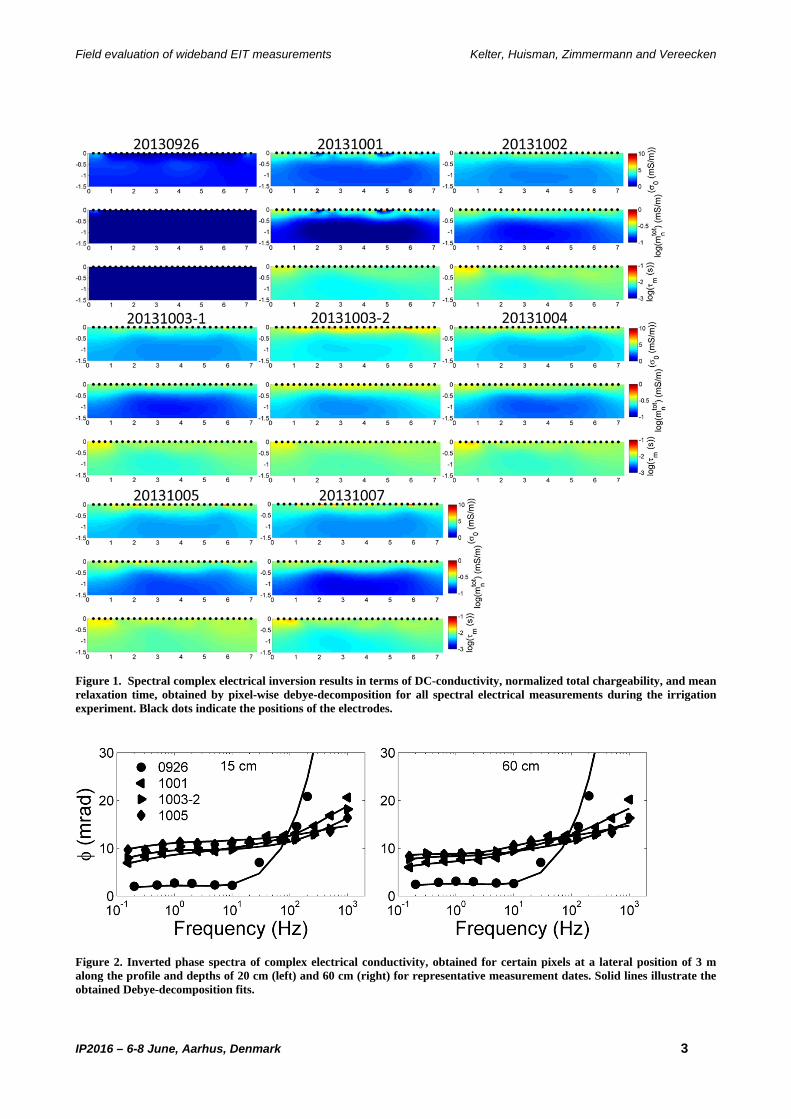
Figure 1 shows a compilation of spectral complex electrical imaging results obtained during and after infiltration. The results clearly show that the electrical conductivity, the normalized total chargeability, as well as the mean relaxation time all increased with increasing soil water content. For all three integral spectral parameters, a clear maximum is obtained for the measurement where stationary flow conditions were assumed (20131003-2), whereas minimum values are obtained for the first measurement in driest conditions. The imaging results also indicate a two layered soil in both the electrical conductivity and normalized total chargeability images. Figure 2 presents inverted phase spectra of complex electrical conductivity for selected pixels. The consistency of the spectra across a broad frequency range is evident, and this confirms the feasibility of wideband spectral EIT for near-surface applications with short cable lengths where inductive coupling can be neglected. Case study II: Aquifer characterization Wideband borehole EIT measurements were made to investigate the well-characterized heterogeneous unconfined aquifer at the Krauthausen test site (Müller et al. 2010). The base of the aquifer is located at a depth of 11 to 13 meter and consists of intermitting layers of clay and silt, whereas the upper part of the aquifer consists of 3 layers with Rur sediments at the top followed by the upper and lower Rhine sediments. In contrast to the first case study, multicore electrode chains as developed in Zhao et al. (2013) were used with an electrode separation of 1 m. EIT measurements were performed using two electrode chains in borehole B75 and B76 using both single well and cross-well electrode configurations. Therefore, calibration measurements and numerical modelling of the cable layout of the electrode chains were used in order to correct for inductive coupling effects. The details of this correction procedure are described in Zhao et al. (2015). Processing and inversion of the measured impedance data was identical to the first case study. Analysis of reciprocal measurements showed that data error was very similar for uncorrected and corrected data. This confirms that errors associated with inductive coupling are of reciprocal nature, as already postulated by Zhao et al. (2015). Figure 3 shows inversion results for the imaginary part of the electrical conductivity at four frequencies for uncorrected and corrected data. In the low frequency range (until 10 Hz), the images of the uncorrected and the corrected data show very similar results, whereas the images of the uncorrected data show increasingly strong artefacts for frequencies higher than 10 Hz. In contrast to the erratic images of the uncorrected data, the corrected data shows the same structures that are present in the lower frequencies and even an increase in the contrast for the high frequencies, indicating the value of spectral information in complex electrical imaging. Spectral electrical images were compared with estimates of clay content and gravel content determined from material extracted during drilling of the wells and showed good agreement.
CONCLUSIONS In this study, we presented wideband EIT measurements obtained in two field studies. The results show that the use of dedicated EIT measurement equipment in combination with calibration measurements and model-based correction methods in addition to appropriate data processing and inversion strategies allow the accurate determination of spectral electrical properties in the mHz to kHz frequency range. In particular, spatially and spectrally consistent
inversion results were obtained up to a frequency of 1 kHz during an infiltration experiment, which illustrated the ability of spectral EIT to monitor near-surface vadose zone processes using surface electrodes and short cables. In the case of aquifer studies that extend beyond the top few meters of the soil, longer cables are required that may lead to unwanted inductive coupling effects. In this study, it was shown that a previously developed combination of calibration measurements and model-based corrections successfully removed inductive coupling effects and provided spatially and spectrally consistent electrical properties up to 1 kHz. Overall, we conclude that wideband spectral EIT has matured to such an extent that routine applications are becoming feasible.
ACKNOWLEDGMENTS We gratefully acknowledge the SFB/TR32 "Patterns in Soil-Vegetation-Atmosphere Systems: monitoring, modeling, and data assimilation“, which is funded by the Deutsche Forschungsgemeinschaft (DFG) for financial support.
REFERENCES Flores Orozco, A., Williams, K.H., Long, P.E., Hubbard, S.S., and Kemna, A., 2011. Using complex resistivity imaging to infer biogeochemical processes associated with bioremediation of an uranium-contaminated aquifer. Journal of Geophysical Research, 116: G03001. M. Kelter M., Huisman, J.A., Zimmermann, E. Kemna, A. Vereecken, H., 2015, Quantitative imaging of spectral electrical properties of variably saturated soil columns, Journal of Applied Geophysics, 123, 333 - 344. Kemna, A. (2000). Tomographic inversion of complex resistivity – theory and application. Ph.D. thesis, Ruhr-University of Bochum, Germany. Kemna, A., Binley, A., Cassiani, G., Niederleithinger, E., Revil, A., Slater, L., and Zimmermann, E., 2012. An overview of the spectral induced polarization method for near-surface applications. Near Surface Geophysics, 10(6), 453-468. Müller, K., Vanderborght, J., Englert, A., Kemna, A., Huisman, J. A., Rings, J., & Vereecken, H., 2010. Imaging and characterization of solute transport during two tracer tests in a shallow aquifer using electrical resistivity tomography and multilevel groundwater samplers. Water Resources Research, 46(3), W03502. Zhao, Y., Zimmermann, E., Huisman, J.A., Treichel, A., Wolters, B., van Waasen, S., Kemna, A., 2013. Broadband EIT borehole measurements with high phase accuracy using numerical corrections of electromagnetic coupling effects. Measurement Science Technology, 24 (8), 085005. Zhao, Y., Zimmermann, E., Huisman, J.A., Treichel, A., Wolters, B., van Waasen, S., Kemna, A., 2015. Phase correction of electromagnetic coupling effects in cross-borehole EIT measurements. Measurement Science Technology, 26 (1), 015801. Zimmermann, E., Kemna, A., Berwix, J., Glaas, W., Vereecken, H., 2008. EIT measurement system with high phase accuracy for the imaging of spectral induced polarization properties of soils and sediments. Measurement Science Technology, 19, 094010.
Field evaluation of wideband EIT measurements Kelter, Huisman, Zimmermann and Vereecken
IP2016 – 6-8 June, Aarhus, Denmark 3
Figure 1. Spectral complex electrical inversion results in terms of DC-conductivity, normalized total chargeability, and mean relaxation time, obtained by pixel-wise debye-decomposition for all spectral electrical measurements during the irrigation experiment. Black dots indicate the positions of the electrodes.
Figure 2. Inverted phase spectra of complex electrical conductivity, obtained for certain pixels at a lateral position of 3 m along the profile and depths of 20 cm (left) and 60 cm (right) for representative measurement dates. Solid lines illustrate the obtained Debye-decomposition fits.

Figure 3. EIT imaging results for frequencies of 2, 10, 100 and 1000 Hz for uncorrected (top) and corrected (bottom) data in terms of the imaginary part of the complex electrical conductivity.

IP2016 – 6-8 June, Aarhus, Denmark 1
3D TEM-IP inversion workflow for galvanic source TEM data
Seogi Kang Douglas W. Oldenburg University of British Columbia University of British Columbia
6339 Stores Rd., Vancouver, Canada 6339 Stores Rd., Vancouver, Canada
[email protected] [email protected]
INTRODUCTION
The electrical conductivity of earth materials can be frequency
dependent with the effective conductivity decreasing with
decreasing frequency due to the buildup of electric charges
that occur under the applied electric field. Effectively, the rock
is electrically chargeable. Controlled-source electromagnetic
(EM) methods excite the earth using either galvanic (a
generator attached to two grounded electrodes) or inductive
source (arising from currents flowing in a wire loop). A typical
EIP survey layout (Siegel, 1959) is shown in Figure 1.
Grounded wire
Figure 1. Conceptual diagram of a ground-based galvanic
source with half-duty cycle current waveform.
It consists of grounded electrodes carrying a current waveform
(like the square wave shown) and electrodes to measure
voltage differences. When the ground is chargeable the
received voltage looks like that in Figure 2. The decay in the
off-time is the IP effect. To interpret observed IP data, a two-
stage inversion is usually deployed (Oldenburg and Li, 1994).
The first step is to invert late on-time data (V0) using a DC
inversion to obtain the background conductivity. The second
step is to use the obtained conductivity to generate a sensitivity
function, and then invert late off-time data (Vs); this is often
called DC-IP inversion.
Figure 2. A typical overvoltage effects in EIP data.
Although application of this method has been successful, a
main concern is the second step. The time decaying fields
are assumed to be purely the result of IP phenomena and any
EM induction effects in the data are ignored. This assumption
can be violated when the earth has a significant conductivity
and EM coupling can remain even in the late off-time.
Removing the effects of EM induction from the measured data
is referred to as EM-decoupling and it has been a focus of
attention for many years. Most analyses have used simple
earth structures: half-space and layered earth to ameliorate its
effects (Wynn and Zonge, 1975). However, with our current
capability to handle 3D forward modelling and inversion it is
timely to revisit this issue.
In a recent work (Kang and Oldenburg, 2016), we developed a
workflow for inverting airborne IP data using inductive
sources. This involved three main steps: a) inverting early time
TEM data to recover a 3D conductivity, b) EM-decoupling
(forward modelling the EM response and then subtracting it
from the observations), and c) IP inversion to recover pseudo-
chargeability distribution at each time channel. The current
problem of inverting IP data using grounded sources follows
the same workflow but some aspects are greatly simplified
because EIP measures data when electric fields, and charge
accumulations, have reached a steady state. This provides
another data set from which information about the electrical
conductivity can be extracted.
A major difference between conventional EIP inversion and
our approach is the use made of early time channels in the EIP
data. In conventional work these have been considered as
“noise” and hence been thrown away. However, we consider
these as “signal” to recover conductivity. In this study, we
apply a 3D TEM-IP inversion workflow to the synthetic
galvanic source example (gradient array). This will include the
three steps in the workflow listed above but the first step is
SUMMARY
Electrical induced polarization (EIP) surveys have been
used to detect chargeable materials in the earth. For
interpretation of the time domain EIP data, the DC-IP
inversion method, which first invert DC data (on-time) to
recover conductivity, then inverts IP data (off-time) to
recover chargeability, has been successfully used
especially for mining applications finding porphyry
deposits. It is assumed that the off-time data are free of
EM induction effects. When this is not the case, an EM-
decoupling technique, which removes EM induction in
the observation, needs to be implemented. Usually
responses from a half-space or a layered earth are
subtracted. Recent capability in 3D TEM forward
modelling and inversion allows us to revisit this
procedure. Here we apply a 3D TEM-IP inversion
workflow to the galvanic source example. This includes
three steps: a) invert DC and early time channel TEM data
to recover the 3D conductivity, b) use that conductivity to
compute the TEM response at later time channels.
Subtract this fundamental response from the observations
to generate the IP response, and c) invert the IP responses
to recover a 3D chargeability. This workflow effectively
removes EM induction effects in the observations and
produces better chargeability and conductivity models
compared to conventional approaches.
Key words: Induced polarization, EM-decoupling,
galvanic source, time domain EM, 3D inversion

3D TEM-IP inversion workflow Seogi Kang and Douglas W. Oldenburg
IP2016 – 6-8 June, Aarhus, Denmark 2
altered so that we invert the DC data, and early time channels
of TEM data, to recover the 3D conductivity.
SEPARATION OF EM AND IP RESPONSE
Assuming the earth has chargeable material, the observed
responses from any TEM survey has both EM and IP
responses. To be more specific, we first define the complex
conductivity in the frequency domain as
(1)
where is the conductivity at infinite frequency, and is
angular frequency (rad/s). For the Cole-Cole model from
Pelton et al. (1978),
, (2)
where is intrinsic chargeability, is time constant, and c is
frequency dependency. Following Smith et al. (1988), the
observed datum including both EM and IP effects can be
defined as
, (3)
where dF and dIP are respectively the fundamental and IP
responses. Here the fundamental response is ,
where F[] is a Maxwell’s operator; this takes the conductivity
and computes EM responses without IP effects. Note that
when =0. A main goal of our 3D TEM-IP
inversion workflow is to evaluate the dF and dIP components.
To illustrate the challenge, we perform a simple TEM forward
modelling using a galvanic source as shown in Figure 1. We
inject a half-duty cycle rectangular current through a grounded
wire. A chargeable body is embedded in the earth. Figure 3
shows the measured voltage at a pair of potential electrodes on
the surface. It is different from the conventional over-voltage
diagram shown in Figure 2. At early on- and off-time, we
observe significant EM induction effects. It is only at late off-
times that we can identify typical over-voltage effects which
are characteristic of the IP responses. The fact that EM
dominates the data at early times and IP effects dominate the
late-time data suggests it may be possible to separate the EM
and IP responses in time.
For a clearer demonstration of this, we view only the off-time
data, and plot them on a log-log plot as shown in Figure 4.
Black, blue, and red lines correspondingly indicate observed,
fundamental, and IP responses; solid and dotted lines
distinguish negative and positive data. At early times, the
fundamental response is much greater than the IP data; this is
the region of EM dominance. At later times, the IP signal is
much greater than the fundamental; this is the region of IP-
dominance. Importantly, there is an intermediate time region
when both EM and IP are considerable. Our following
inversion workflow is based upon this natural separation of
EM and IP in time.
3D TEM-IP INVERSION WORKFLOW
Our inversion workflow is based upon Kang and Oldenburg
(2016) which was built for an inductive source case, but is
applicable here. Figure 5 shows the 3D TEM-IP inversion
workflow to be applied. The first step is to invert the TEM data
to recover the 3D model. As in our inductive source
work, we use only early time data that we feel are not IP-
contaminated. We note that these early time data have
previously been considered as “noise” in conventional
analyses and hence have been thrown away. However, here we
consider these as “signal” and use them to recover a better
conductivity model. Another possibility for obtaining a
background conductivity is to use the steady-state fields just
prior to switching the current off. These are the potentials that
are traditionally used in DC-IP inversion. Inversion of these
data yields a conductivity that is but if is
small enough then this will be a reasonable approximation to
. The inversion of DC data is analogous to inverting only
one frequency in a frequency-domain data set. Hence it might
be expected that inverting data at multi-times (equivalent to
multi-frequencies) would produce a better result. Our
experience verifies this. Nevertheless, the DC fields are
valuable and we wish to use them. The options are to invert the
DC and TEM data together, or treat them as two separate data
sets. For the present we have chosen the latter since we then
do not have to contend with the issue that the DC fields are
really . The approach implemented here is first to invert the
DC data and then use the resulting model as a starting and
reference model for the TEM inversion
Figure 3. Observed voltage with EM induction effects. EM
effects dominate the early off-time data.
EM
Induction
Intermediate
IP
Figure 4. Transients of observed (black line), fundamental
(blue crosses) and IP (red line) at the off-time in the log-log
plot. Solid and dotted lines distinguish positive and
negative datum.
The second step of the workflow is EM decoupling. The
estimated conductivity model, est, from step 1 is used to
generate raw IP data according to
, (4)
where dobs is the observed data, F [est] is estimated
fundamental data. Here, we identify that the predicted
fundamental response might be different from true
fundamental response, because est is not the same as .
Potential errors in raw IP data will be significant especially at
early times, but they will decrease as time increases. The
effective region for EM-decoupling will be in the intermediate
time when both EM and IP are considerable (Figure 4). Note

3D TEM-IP inversion workflow Seogi Kang and Douglas W. Oldenburg
IP2016 – 6-8 June, Aarhus, Denmark 3
that at late time (IP-dominant) EM-decoupling may not be
required.
The final step in the process is to carry out the IP inversion.
We adopt the conventional IP inversion approach (e.g.
Oldenburg and Li, 1994), which uses a linear form of IP
responses written as
, (5)
where G is the sensitivity function and is the pseudo-
chargeability. The conductivity model est is required to
generate the sensitivity matrix. We invert each time channel
of IP data separately, and recover pseudo-chargeability at
multiple times. Interpreting this recovered pseudo-
chargeability to extract intrinsic IP information such as , ,
and c is possible, but we do not treat that in this study.
Figure 5. A 3D TEM-IP inversion workflow for galvanic
source TEM data.
GALVANIC SOURCE EXAMPLE
Synthetic TEM data
As an example, we use a galvanic source and multiple
receivers which measures voltages as shown in Figure 3. Four
blocks (A1-A4) presented in Figure 6 have different and
values (see Table 1); all blocks have =0.5 sec and c=1
(Debye model). Only A2 and A3 blocks are chargeable. The
length of the transmitter wire is 4.5 km and potential
differences between two electrodes along easting lines are
measured at 625 locations. The measured time channels are
logarithmic-based ranging from 1-600 ms (60 channels).
Computed responses at 5, 80, and 350 ms are shown in Figure
7. At 5 ms, EM induction effects are dominant, and all data are
negative. At 80 ms, both EM and IP effects are considerable,
but still all data are negative. Note that A2 and A3 are
chargeable, but A1, which is conductive, is not. Therefore, it is
difficult to differentiate chargeability and conductivity
anomalies just by looking at observed data at 80 ms. At 350
ms, EM induction effects are significantly decayed, hence IP is
dominant. Only A2 and A3 show positive anomalies that
originate from chargeability. Depending on the measured time
window, and IP parameters of chargeable bodies, we could
have data in IP-dominant time or not. Hence, whenever our
measured time window is not late enough to be considered as
IP-dominant time, EM-decoupling is crucial step. Note that the
A1 anomaly at 80 ms could be misinterpreted as a chargeable
response, if this is the latest time channel.
Table 1. Conductivity at infinite frequency and intrinsic
chargeability values for five units: A1-A4 and half-space.
3D DC and TEM inversion
To recover , we use the first six channels of the TEM data
(1-6 ms), which have minor contamination from IP. In
addition, we have DC data which contain IP effects, but have
minor EM induction effects. We first invert the DC data, and
recover 3D conductivity. By using the recovered DC
conductivity as a reference model, we invert the TEM data.
The recovered conductivity models from the 3D DC and TEM
inversions are shown in Figure 8. The conductive blocks A1
and A3 are much better imaged with the TEM inversion.
A1 A2
A3 A4
A1 A2
A3 A4
Figure 6. Plan and section views of the 3D mesh. Black
solid lines show the boundaries of four blocks (A1-A4).
Only A2 and A3 are chargeable. Arrows indicate a wire
path for the galvanic source.
5 ms 80 ms 350 ms
A1 A2
A3 A4
A1 A2
A3 A4
A1 A2
A3 A4
Figure 7. Plan maps of the observed TEM data at 5 ms (left
panel), 80 ms (middle panel), 350 ms (right panel). Dashed
and solid contours differentiate negative and positive data.
A1 A2
A3 A4
A1
A3 A4
(a) DC inversion
A1 A2
A3 A4
A1
A3 A4
(b) TEM inversion
Figure 8. Recovered conductivity models from (a) DC and
(b) TEM inversions.
EM-decoupling
3D TEM-IP inversion workflow Seogi Kang and Douglas W. Oldenburg
IP2016 – 6-8 June, Aarhus, Denmark 4
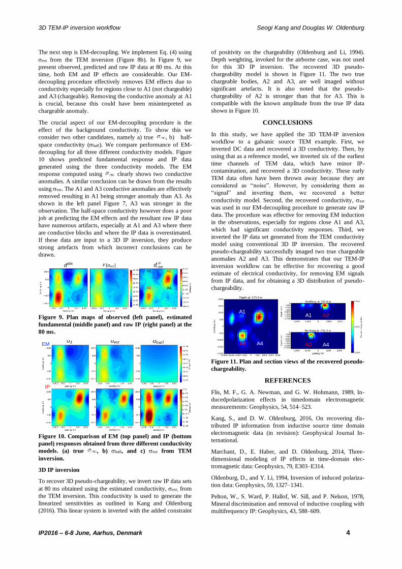
The next step is EM-decoupling. We implement Eq. (4) using
est from the TEM inversion (Figure 8b). In Figure 9, we
present observed, predicted and raw IP data at 80 ms. At this
time, both EM and IP effects are considerable. Our EM-
decoupling procedure effectively removes EM effects due to
conductivity especially for regions close to A1 (not chargeable)
and A3 (chargeable). Removing the conductive anomaly at A1
is crucial, because this could have been misinterpreted as
chargeable anomaly.
The crucial aspect of our EM-decoupling procedure is the
effect of the background conductivity. To show this we
consider two other candidates, namely a) true , b) half-
space conductivity (half). We compare performance of EM-
decoupling for all three different conductivity models. Figure
10 shows predicted fundamental response and IP data
generated using the three conductivity models. The EM
response computed using clearly shows two conductive
anomalies. A similar conclusion can be drawn from the results
using est. The A1 and A3 conductive anomalies are effectively
removed resulting in A1 being stronger anomaly than A3. As
shown in the left panel Figure 7, A3 was stronger in the
observation. The half-space conductivity however does a poor
job at predicting the EM effects and the resultant raw IP data
have numerous artifacts, especially at A1 and A3 where there
are conductive blocks and where the IP data is overestimated.
If these data are input to a 3D IP inversion, they produce
strong artefacts from which incorrect conclusions can be
drawn.
A1 A2
A3 A4
dobs dI Pr awF [σest ]
Figure 9. Plan maps of observed (left panel), estimated
fundamental (middle panel) and raw IP (right panel) at the
80 ms.
EM
IP
σ1 σest σhal f
Figure 10. Comparison of EM (top panel) and IP (bottom
panel) responses obtained from three different conductivity
models. (a) true , b) half, and c) est from TEM
inversion.
3D IP inversion
To recover 3D pseudo-chargeability, we invert raw IP data sets
at 80 ms obtained using the estimated conductivity, est, from
the TEM inversion. This conductivity is used to generate the
linearized sensitivities as outlined in Kang and Oldenburg
(2016). This linear system is inverted with the added constraint
of positivity on the chargeability (Oldenburg and Li, 1994).
Depth weighting, invoked for the airborne case, was not used
for this 3D IP inversion. The recovered 3D pseudo-
chargeability model is shown in Figure 11. The two true
chargeable bodies, A2 and A3, are well imaged without
significant artefacts. It is also noted that the pseudo-
chargeability of A2 is stronger than that for A3. This is
compatible with the known amplitude from the true IP data
shown in Figure 10.
CONCLUSIONS
In this study, we have applied the 3D TEM-IP inversion
workflow to a galvanic source TEM example. First, we
inverted DC data and recovered a 3D conductivity. Then, by
using that as a reference model, we inverted six of the earliest
time channels of TEM data, which have minor IP-
contamination, and recovered a 3D conductivity. These early
TEM data often have been thrown away because they are
considered as “noise”. However, by considering them as
“signal” and inverting them, we recovered a better
conductivity model. Second, the recovered conductivity, est
was used in our EM-decoupling procedure to generate raw IP
data. The procedure was effective for removing EM induction
in the observations, especially for regions close A1 and A3,
which had significant conductivity responses. Third, we
inverted the IP data set generated from the TEM conductivity
model using conventional 3D IP inversion. The recovered
pseudo-chargeability successfully imaged two true chargeable
anomalies A2 and A3. This demonstrates that our TEM-IP
inversion workflow can be effective for recovering a good
estimate of electrical conductivity, for removing EM signals
from IP data, and for obtaining a 3D distribution of pseudo-
chargeability.
A1 A2
A3 A4
A1
A3 A4
A2
Figure 11. Plan and section views of the recovered pseudo-
chargeability.
REFERENCES
Flis, M. F., G. A. Newman, and G. W. Hohmann, 1989, In-
ducedpolarization effects in timedomain electromagnetic
measurements: Geophysics, 54, 514–523.
Kang, S., and D. W. Oldenburg, 2016, On recovering dis-
tributed IP information from inductive source time domain
electromagnetic data (in revision): Geophysical Journal In-
ternational.
Marchant, D., E. Haber, and D. Oldenburg, 2014, Three-
dimensional modeling of IP effects in time-domain elec-
tromagnetic data: Geophysics, 79, E303–E314.
Oldenburg, D., and Y. Li, 1994, Inversion of induced polariza-
tion data: Geophysics, 59, 1327–1341.
Pelton, W., S. Ward, P. Hallof, W. Sill, and P. Nelson, 1978,
Mineral discrimination and removal of inductive coupling with
multifrequency IP: Geophysics, 43, 588–609.

3D TEM-IP inversion workflow Seogi Kang and Douglas W. Oldenburg
IP2016 – 6-8 June, Aarhus, Denmark 5
Seigel, H., 1959, Matehmatical formulation and type curves for
induced polarization: Geophysics, 24, 547–565.
Smith, R. S., P. Walker, B. Polzer, and G. F. West, 1988, The
time-domain electromagnetic response of polarizable bodies:
an approximate convolution algorithm: Geophysical
Prospecting, 36, 772–785.
Weidelt, P., 1982, Response characteristics of coincident loop
transient electromagnetic systems: 47, 1325–1330.
Wynn, J. C., and K. L. Zonge, 1975, EM coupling, its intrinsic
value, its removal and the cultural coupling problem: Geo-
physics, 40, 831–85

IP2016 – 6-8 June, Aarhus, Denmark 1
Methods for measuring the complex resistivity spectra of rock
samples in the context of mineral exploration Tina Martin Stephan Costabel Thomas Günther Federal Institute for Geosciences Federal Institute for Geosciences Leibniz Institute for Applied and Natural Resources (BGR) and Natural Resources (BGR) Geophysics (LIAG)
Wilhelmstr. 25-30 Wilhelmstr. 25-30 Stilleweg 2, D-13593 Berlin/Germany D-13593 Berlin/Germany D-30655 Hannover/Germany
[email protected] [email protected] [email protected]
INTRODUCTION
Critical raw materials such as Sn, W, In and rare earth metals
are very important today for producing electronic equipment. In the past decades the exploration activities in Germany for
mineral resources were low and therefore the research in this
field. Nowadays efforts are undertaken to develop new
technologies and exploration systems (e.g. using helicopter electromagnetics as in the project, where this work is involved
in). Along with the geophysical exploration, it becomes
important to know about petrology and the genesis of the
expected mineral deposits and the knowledge about petrophysical characterization of the rocks involved are
essential.
This information can then be used for improving (three-
dimensional) images of the electrical resistivity distribution in the subsurface and can thus provide indications of mineralized
deposits and their geological, tectonic, and structural properties.
The main focus in the current research project are antimonite deposits. To measure petrophysical parameters such as density,
resistivity and magnetic susceptibility, samples of antimonite and the deposit surrounding material are required. However, at
least in Germany, in situ samples cannot be obtained anymore
due to closed mining pits. Only existing samples in rock
collections are available. The problem is that it is mostly not allowed to destroy or cut these samples so new approaches for
measuring of the complex resistivity have to be developed. The
following study demonstrate preliminary results of potential strategies to overcome the given limitations.
MATERIAL AND METHODS Most of the samples in geological rock collections have an
approximate size of a fist and exhibit arbitrary geometries (Figure 1). It is usually not allowed or even possible to drill
cylindrical samples matching a common four-point measuring
cell for measuring the complex resistivity, because the samples
are too precious, too small or too instable. For a reliable data acquisition, three different approaches are pursued:
1.) If possible, cylindrical core samples are measured in the
measuring cell.
2.) Fist-sized samples with irregular geometry are measured
using small (nail) electrodes stuck on the rock surface.
3.) Samples with irregular geometry are buried in a sandboxes
for measuring exact phase values.
Figure 1: Picture of an antimonite from the BGR rock
collection.
For measuring the complex resistivity * we use an SIP
(spectral induced polarization) instrument (SIP-ZEL,
Zimmermann et al., 2008), which provides magnitude (||) and
SUMMARY
For the geophysical exploration of mineral resources
knowledge about petrophysical parameters of the expected
investigation material is essential. If it is not possible to measure samples in a common geometry, new approaches
have to be developed. In this preliminary study three
approaches for adequate and proper measurements of
spectral induced polarization at rock samples are introduced.
First results show that additionally to the measurement in
a common 4-point measuring cell, also measurements with
stuck electrodes connected to rock samples with irregular geometry seem to be promising. Furthermore the detection
of a buried antimonite sample in a sand-box could be
demonstrated by the strong phase anomaly it produced.
Nevertheless further investigations are necessary, such as considering possible anisotropy effects and verification of
the methods for a broader range of samples with irregular
geometry. Also the electrode material for the
measurements in the sandbox should be modified to avoid unwanted polarization effects. In addition, alternative
materials for coupling the electrodes directly to the rock
surface will be tested in the future.
Key words: SIP, laboratory measurement, hard rock
sample, arbitrary geometry, antimonite

SIP at rock samples Martin, Costabel and Günther
IP2016 – 6-8 June, Aarhus, Denmark 2
phase () of the complex resistivity. These parameters are
related to the real ( )́ and imaginary (´´) parts of resistivity by
𝜌∗ = |𝜌|𝑒𝑖𝜑 = 𝜌′ + 𝜌′′ = 1
𝜎 ∗
with * being the electrical conductivity. The magnitude (||)
and the phase () are associated with:
|𝜌| = √𝜌′2 + 𝜌′′2
and
𝜑 = arctan [𝜌′′
𝜌′ ].
1.) Cylindrical core samples
For the laboratory measurements we use a four-point measuring
cell (Figure 2Figure 2 a) with stainless steel current electrodes at the face side of the cell and potential electrodes (Ni-Co alloy)
being ring wires placed outside the electrical field in the central
part of the cell (more information in Kruschwitz 2008).
The core samples were drilled in cylindrical shape with 2 cm in diameter and various lengths (Figure 2Figure 2 b). The cores
were extracted from two different directions to consider
possibly occurring anisotropy effects and are measured under
controlled conditions in a climatic chamber (20°C) at a frequency range between 2 mHz and 45 kHz. As coupling agent
we used an Agar-Agar gel.
The complex resistivity * is then calculated by
𝜌∗ = 𝑅𝐴
𝐿
where R is the measured resistance. The ratio A/L is the
geometric factor of the sample holder with the length L between
the potential electrodes and the cross-section area A.
Figure 2: a) 4-point measuring cell. b) Cylindrical core
samples from antimonite.
2.) Measurements using stuck electrodes
To measure the complex resistivity at the fist-size samples small holes (< 2 mm) were drilled. Silver wire electrodes were
stuck with conductive epoxy or silverpaint (very well
conducting glue) at the sample. At least four electrodes are
needed for a measurement (Figure 3). In our first tests, the electrodes are placed in line with a distance of about 1 cm to
each other. To consider the anisotropy of the samples further
electrodes on each side are possible.
Figure 3: Picture of a rock sample with stuck electrodes.
To digitize the geometry and to calculate the geometry factor
the samples are scanned by a 3-D scanner (Matter and Form,
2016). It provides a high resolution and also photographic recording (Figure 4). With the exact geometry and the position
of the electrodes the necessary factors are calculated using a
tetrahedral Finite-Element mesh that is generated from the
surface mesh with the mesh generator TetGen (Rücker et al., 2006).
Figure 4: Results from 3-D scan. a) Photographic, b) 3-D
scan points, c) connection between the scanned points.
3.) Measurements in a sandbox
To measure exact phase values, the fist-sized samples were also
buried in a sandbox (44 x 25 x 25 cm) filled with pure fully
saturated quartz sand. A principal feasibility study could be shown by Radic (1984).
Newer result (for the detection of tree roots) can be found in
Zanetti et al. (2011).
In our previous studies this sand showed negligible phase
effects and resistivities in the range of 45 m (fluid
conductivity: 700 µS/cm/14.3 m). Due to the limited size of
the sandbox boundary effects may occur and therefore resistivity can be overestimated.
We used 12 stainless steel nails as electrodes, which are
arranged in line with a distance of 3 cm (Figure 5), so different
measurement arrays with varying depth levels and multi-channel recording are possible. An inversion of the data can be
done with the BERT algorithm (Günther et al, 2006). To
account for the geometry of the tank, we use a hybrid 2D/3D
approach, i.e. a 3D forward calculation is combined with a 2D inversion (Ronczka et al., 2014).
Formatted: Font: Times New Roman, 9 pt

SIP at rock samples Martin, Costabel and Günther
IP2016 – 6-8 June, Aarhus, Denmark 3
Figure 5: Picture of the sandbox with electrode line.
RESULTS AND DISCUSSION
1.) Cylindrical core samples
Example spectra of antimonite core samples are shown in Figure 6. All five rock samples were cut from one rock sample
but with perpendicular orientation (orientation A: 1 and 2;
orientation B: 3, 4 and 5). The resistivity values (left) are
clustered: two samples exhibit higher resistivities (10 000 m)
and three exhibit lower values (~ 2000 m). Unfortunately this
observation cannot be fully related to the orientation. In
contrast, the phase values can be related to the orientation: higher phases (10 mrad) are associated with orientation B and
lower (5 mrad) values with A. However, in general the phases
are relatively small and their behaviour over the entire
frequency range is more or less constant, except for high frequencies, which is assumed to be an artefact caused by
unavoidable inductive effects of the measurement setup.
Figure 6: First results of an antimonite core samples.
Sample 1 and 2 are perpendicular to 3, 4, and 5.
2.) Measurements using stuck electrodes In Figure 7 the preliminary results for an SIP measurement with stuck electrodes at a fist-sized antimonite sample is shown. The
coupling resistance between current and potential electrodes
was sufficiently small with < 3 kAs a preliminary estimate, the geometry factor was calculated assuming the four-point-
electrode line over a halfspace, which yields at least a rough
estimation of the order of magnitude for the resistivity of the
rock. In future, the calculation of the geometry factor will be repeated by simulated resistance measurements using the
digitized 3-D model. However, the preliminary resistivity
estimate of the investigated sample is in principal agreement
with the core samples around 2000 m. In contrast to the core samples, we observe no phase effects, only a continuous
increase from low to high frequencies that appears to be linear
when plotted using a log-log scaling, which indicates inductive
effects from the measurement system.
Figure 7: First results of a fist-sized sample of antimonite
with stuck electrodes (two repetitions).
3.) Measurements in a sandbox
Various measurements in the sandbox were carried out. To
characterize the filling sand after saturation with water
(700 µS/cm), it was measured first in the four-point measuring cell. After filling the sandbox, the water-saturated sand was
measured again with two different arrays (Wenner-alpha and
dipole-dipole). At least for small electrode distances (first
level), the resistivity measurement in the sandbox corresponded to the reference measurement in the cell. For higher levels, the
boundary of the sandbox caused an overestimation of the
resistivity. On the other hand, the zero-phase in the sandbox
was only found for the higher levels, while a peak with a maximum between 2 and 38 mrad at frequencies between 0.1
and 1 Hz in the phase spectrum was found for the first levels. It
is contemplated whether this artefact is associated with
polarizing effects at the steel electrodes. After the reference measurements using the pure sand, a fist-
sized native antimonite sample was buried in the centre of the
sandbox (just below electrodes 6, 7 and 8) at a depth between 3 and 7 cm. In Figure 8 the results of these measurements using a
Wenner-alpha array are shown. At the electrodes 5, 6, 7 and 8
(red open triangle), resistivities of about 45 m and very small
phase values were measured corresponding to the pure sand characteristics. One electrode position further (6, 7, 8, 9 orange
triangle), a remarkable phase effect (up to 300 mrad) could be
observed with a maximum at 100 Hz. This phase effect is
increasing with increasing electrode distances (equivalent to depth) and is associated with the buried antimonite sample,
while the resistivity value does hardly show a significant
change. For the highest level (green open square) the resistivity
is overestimated probably because of the limited dimension of the sandbox, which was already observed for the measurements
in the pure sand before. The next step is an inversion of the data
that considers the correct dimensions of the sandbox.
Figure 8: First results from a buried antimonite in fully
saturated quartz sandbox.
SIP at rock samples Martin, Costabel and Günther
IP2016 – 6-8 June, Aarhus, Denmark 4
CONCLUSIONS
Our preliminary results show that probably reliable SIP measurements can be carried out using any of the three
approaches. Previous studies (e.g., Binley et al., 2005;
Kruschwitz, 2008; Martin, 2010; Weller et al., 2011)
demonstrate that measurements at cylindrical core samples in a four-point cell can be considered to be the state-of-the-art for
solid rocks.
However, also measurements at rock samples with irregular
geometry seems to be a promising tool, even if there is still potential to further develop the proposed approaches.
SIP measurements at sand-filled boxes can also be a suitable
way. However, the reliability of the SIP characterization of
buried rocks inside a box must be verified in further studies. Our next steps are the comparison of the three approaches
considering possible anisotropy effects and the verification of
the measurement for a broader range of samples with irregular
geometry. The electrode material for the measurements in the sandbox should be modified to avoid unwanted polarization
effects. Also, alternative materials for coupling the electrodes
directly to the rock surface will be tested in the future.
ACKNOWLEDGMENTS We thank the German Ministry of Education and Research
(BMBF) for funding the project DESMEX (grant 033R130A)
in which all the work is done. We also thank the BGR technicians for their great support.
REFERENCES
Binley A., Slater L., Fukes M. and Cassiani G., 2005. The
relationship between spectral induced polarization and
hydraulic properties of saturated and unsaturated sandstone. Water Resources Research 41(12), W12417, doi:
10.1029/2005WR004202.
Günther, T., Rücker, C., and Spitzer, K. (2006). Three-
dimensional modeling and inversion of DC resistivity data incorporating topography - Part II: Inversion. Geophys. J. Int.,
166, 506-517. doi:10.1111/j.1365-246X.2006.03011.x.
Kruschwitz, S., 2008, Assessment of the complex resistivity behaviour of salt affected building materials: Ph.D. Thesis,
Federal Institute for Materials Research and Testing (BAM).
Martin, T., 2010. Complex resistivity measurements on oak. European Journal of Wood and Wood Products 70, 45-53.
Matter and Form, 2016, https://matterandform.net/scanner
Radic, T., 1984. Bau und Programmierung eines mikrocomputergesteuerten digitalen Messgerätes zur
Bestimmung des komplexen Gesteinswiderstandes durch
induzierte Polarisation und dessen Erprobung im sandgefüllten
Trog. Diploma Thesis (in German), Free University Berlin.
Ronczka, M., Günther, T. and Stoeckl, L. (2014): Geoelectrical
monitoring of freshwater-saltwater interaction in physical
model experiments. Ext. Abstr., 23rd Saltwater Intrusion Meeting, Husum, Germany.
Rücker, C., Günther, T. and Spitzer, K., 2006. 3-D modeling
and inversion of DC resistivity data incorporating topography - Part I: Modeling. - Geophys. J. Int., 166, 495-505.
Weller A., Breede K., Slater L. and Nordsiek S., 2011. Effect
of changing water salinity on complex conductivity spectra of sandstones. Geophysics 76(6), F315-F327.
Zanetti, C., Weller, A., Vennetier, M. and Meriaux, P. (2011)
Detection of buried tree root samples by using geoelectric measurements: a laboratory experiment. Plant and Soil, 339,
273–283.
Zimmermann, E., Kemna, A., Berwix, J., Glaas, W., Münch, H., and Huisman, J., 2008. A high-accuracy impedance
spectrometer for measuring sediments with low polarizability.
Meas. Sci. Technol. 19. doi:10.1088/0957-0233/19/9/094010.
IP2016 – 6-8 June, Aarhus, Denmark 1
Spectral induced polarization in a sandy medium containing semiconductor materials: study of the polarization mechanism ABDULSAMAD Feras FLORSCH Nicolas CAMERLYNCK Christian Sorbonne Université, UPMC-CNRS Sorbonne Université, UPMC-IRD Sorbonne Université, UPMC-CNRS UMR 7619 METIS, Paris, France UMI 209 UMMISCO, Paris, France UMR 7619 METIS, Paris, France [email protected] [email protected] [email protected]
I
NTRODUCTION For a long time, the interpretation of spectral induced polarization has been based on empirical models (Cole and Cole 1941), wherein the physical meanings of the model parameters are difficult to interpret physically. Pioneers like Pelton et al. (1978) showed relationships between chargeability and mineral content in sulphide deposits, but did not provide mechanistic approaches. However several theorists, for instance Schwarz (1962), Wong (1979) and more recently Revil et al. (2015) have proposed mechanistic approaches that light the micro-meso-macro IP in various cases. One consensus does exist regarding the dependence of the time constant with the grain size and the diffusion coefficient (D in m2/s) of ions in the pore solution. However it seems not applicable in the case of semi-conductor particles: the diffusion coefficient as numerically derived from the time constant is some orders of magnitude larger than in the case of siliciclastic mediums (Gurin et al. 2015; Revil et al. 2015). In the presence of electronic semi-conductors, Gurin et al. (2015) and Hupfer et al. (2016) prefer to introduce the notion of specific surface area to model the time constant, and D is no more involved in the relationship providing the time constant.
METHOD AND EXPERIMENTAL RESULTS The complex resistivity of unconsolidated siliciclastic medium containing electron-based semi-conductors minerals were acquired over a frequency range from 91.5 mHz to 20 kHz using SIP Fuchs III electrical impedance spectrometer. We use Fontainebleau sand (consisting of 98 % of pure silica). The particle size lies between (0.1- 0.2 mm). According to our tests, this medium shows a weak polarization, in agreement with all previous works made on such samples. The measurements tank is rectangular with dimensions (28 cm long, 10 cm wide and 10 cm of height). We use a Wenner array with 6.5 cm spacing. Non-polarizable Cu/CuSO4 electrodes are used to measure the potential difference, whereas the current electrodes are made of stainless steel (Ag 316L) electrodes. The metallic grains are randomly scattered throughout the medium. We firstly vary the metal content (mass fraction) and the grain size, and secondly the electrolyte type (sodium chloride NaCl, potassium chloride KCl and sodium sulphate Na2SO4 separately). Finally the electrolyte concentration is also changed with 0.001, 0.01, 0.1 and 0.5 mol/l respectively. The chargeability M of the medium is calculated from the amplitude of the complex resistivity at higher and lower frequencies and the time constant τ is derived from the critical frequency (the frequency of the phase peak).
SUMMARY Induced polarization (IP) is useful for mineral exploration. In the presence of sulphides (more generally speaking: semi-conductors), the charge carriers inside particles are electrons and electron gaps. The inner diffusivity and the charge concentration are very high with respect to the background solution ones. Mechanisms of induced polarization are still under questioning in those cases. In order to improve our knowledge about the mechanisms controlling IP in such mediums, we propose new lab experiments on unconsolidated mineralized medium and begin numerical modelling by using the Poisson-Nernst-Planck (PNP) equation set as well. Four different types of semi-conductors (graphite, pyrite, chalcopyrite and galena) are involved in the experiments. The polarization effect of grain size, mineral concentration as well as electrolyte salinity and type are investigated at the lab scale. We find that the total chargeability of the medium is a function of the mineral volume but is independent of the electrolyte salinity and electrolyte type. However, the time constant (τ) is highly dependent on the grain size and the electrolyte salinity, and is slightly dependent on the mineral type. These results appear to be in agreement with the classical Wong’s theory, but we assume here that no significant redox phenomenon does happen at the grain surface. The observed dependence of the chargeability and the time constant on the salinity could be explained by considering the mineral grain as a dipole impacting the potential and consequently charge distribution in its vicinity. This dipole is generated inside the particle to compensate the primary electrical field and the whole particle is –as a first approximation- a spherical boundary (and volume) with a constant potential on (and in) it. The distribution of the charged particles in the area around the dipole electric will respond accordingly to this boundary condition and is driven by the potential. Since the equations are coupled, the potential depends on return on the resulting ions distribution. Although the finite-element numerical approach used here is still preliminary, it opens wide perspectives in the understanding of IP in more complex media. Key words: spectral induced polarization, electrolyte effect, mineralized medium.
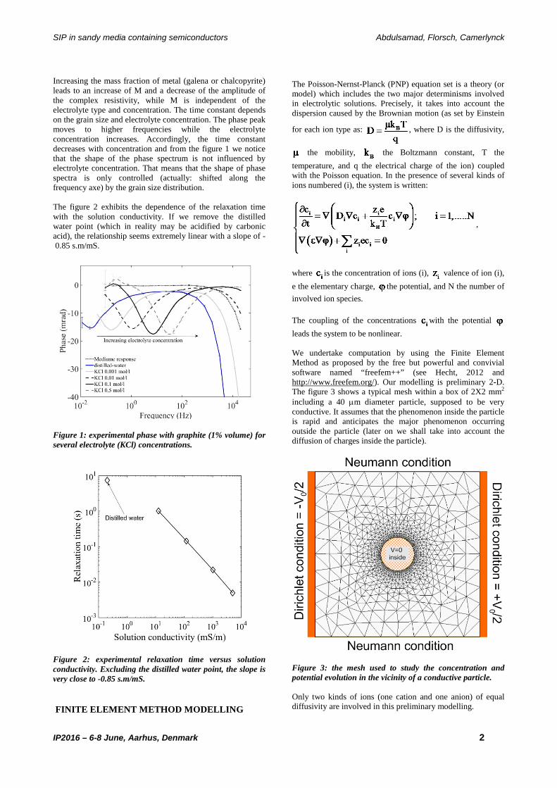
SIP in sandy media containing semiconductors Abdulsamad, Florsch, Camerlynck
IP2016 – 6-8 June, Aarhus, Denmark 2
Increasing the mass fraction of metal (galena or chalcopyrite) leads to an increase of M and a decrease of the amplitude of the complex resistivity, while M is independent of the electrolyte type and concentration. Τhe time constant depends on the grain size and electrolyte concentration. The phase peak moves to higher frequencies while the electrolyte concentration increases. Accordingly, the time constant decreases with concentration and from the figure 1 we notice that the shape of the phase spectrum is not influenced by electrolyte concentration. That means that the shape of phase spectra is only controlled (actually: shifted along the frequency axe) by the grain size distribution. The figure 2 exhibits the dependence of the relaxation time with the solution conductivity. If we remove the distilled water point (which in reality may be acidified by carbonic acid), the relationship seems extremely linear with a slope of - 0.85 s.m/mS.
Figure 1: experimental phase with graphite (1% volume) for several electrolyte (KCl) concentrations.
Figure 2: experimental relaxation time versus solution conductivity. Excluding the distilled water point, the slope is very close to -0.85 s.m/mS. FINITE ELEMENT METHOD MODELLING
The Poisson-Nernst-Planck (PNP) equation set is a theory (or model) which includes the two major determinisms involved in electrolytic solutions. Precisely, it takes into account the dispersion caused by the Brownian motion (as set by Einstein
for each ion type as: , where D is the diffusivity,
the mobility, the Boltzmann constant, T the
temperature, and q the electrical charge of the ion) coupled with the Poisson equation. In the presence of several kinds of ions numbered (i), the system is written:
,
where is the concentration of ions (i), valence of ion (i),
e the elementary charge, the potential, and N the number of
involved ion species.
The coupling of the concentrations with the potential
leads the system to be nonlinear. We undertake computation by using the Finite Element Method as proposed by the free but powerful and convivial software named “freefem++” (see Hecht, 2012 and http://www.freefem.org/). Our modelling is preliminary 2-D. The figure 3 shows a typical mesh within a box of 2X2 mm2 including a 40 µm diameter particle, supposed to be very conductive. It assumes that the phenomenon inside the particle is rapid and anticipates the major phenomenon occurring outside the particle (later on we shall take into account the diffusion of charges inside the particle).
Figure 3: the mesh used to study the concentration and potential evolution in the vicinity of a conductive particle. Only two kinds of ions (one cation and one anion) of equal diffusivity are involved in this preliminary modelling.
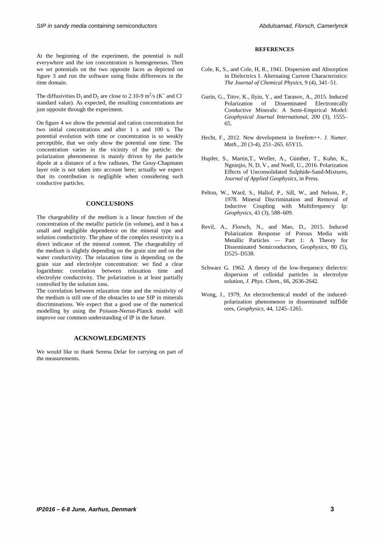
SIP in sandy media containing semiconductors Abdulsamad, Florsch, Camerlynck
IP2016 – 6-8 June, Aarhus, Denmark 3
At the beginning of the experiment, the potential is null everywhere and the ion concentration is homogeneous. Then we set potentials on the two opposite faces as depicted on figure 3 and run the software using finite differences in the time domain. The diffusivities D1 and D2 are close to 2.10-9 m2/s (K+ and Cl-
standard value). As expected, the resulting concentrations are just opposite through the experiment. On figure 4 we show the potential and cation concentration for two initial concentrations and after 1 s and 100 s. The potential evolution with time or concentration is so weakly perceptible, that we only show the potential one time. The concentration varies in the vicinity of the particle: the polarization phenomenon is mainly driven by the particle dipole at a distance of a few radiuses. The Gouy-Chapmann layer role is not taken into account here; actually we expect that its contribution is negligible when considering such conductive particles.
CONCLUSIONS The chargeability of the medium is a linear function of the concentration of the metallic particle (in volume), and it has a small and negligible dependence on the mineral type and solution conductivity. The phase of the complex resistivity is a direct indicator of the mineral content. The chargeability of the medium is slightly depending on the grain size and on the water conductivity. The relaxation time is depending on the grain size and electrolyte concentration: we find a clear logarithmic correlation between relaxation time and electrolyte conductivity. The polarization is at least partially controlled by the solution ions. The correlation between relaxation time and the resistivity of the medium is still one of the obstacles to use SIP in minerals discriminations. We expect that a good use of the numerical modelling by using the Poisson-Nernst-Planck model will improve our common understanding of IP in the future.
ACKNOWLEDGMENTS We would like to thank Serena Delar for carrying on part of the measurements.
REFERENCES
Cole, K, S., and Cole, H, R., 1941. Dispersion and Absorption
in Dielectrics I. Alternating Current Characteristics: The Journal of Chemical Physics, 9 (4), 341–51.
Gurin, G., Titov, K., Ilyin, Y., and Tarasov, A., 2015. Induced
Polarization of Disseminated Electronically Conductive Minerals: A Semi-Empirical Model: Geophysical Journal International, 200 (3), 1555–65.
Hecht, F., 2012. New development in freefem++. J. Numer.
Math., 20 (3-4), 251–265. 65Y15. Hupfer, S., Martin,T., Weller, A., Günther, T., Kuhn, K.,
Ngninjio, N, D, V., and Noell, U., 2016. Polarization Effects of Unconsolidated Sulphide-Sand-Mixtures, Journal of Applied Geophysics, in Press.
Pelton, W., Ward, S., Hallof, P., Sill, W., and Nelson, P.,
1978. Mineral Discrimination and Removal of Inductive Coupling with Multifrequency Ip: Geophysics, 43 (3), 588–609.
Revil, A., Florsch, N., and Mao, D., 2015. Induced
Polarization Response of Porous Media with Metallic Particles — Part 1: A Theory for Disseminated Semiconductors, Geophysics, 80 (5), D525–D538.
Schwarz G. 1962. A theory of the low-frequency dielectric
dispersion of colloidal particles in electrolyte solution, J. Phys. Chem., 66, 2636-2642.
Wong, J., 1979, An electrochemical model of the induced-
polarization phenomenon in disseminated sulfide ores, Geophysics, 44, 1245–1265.
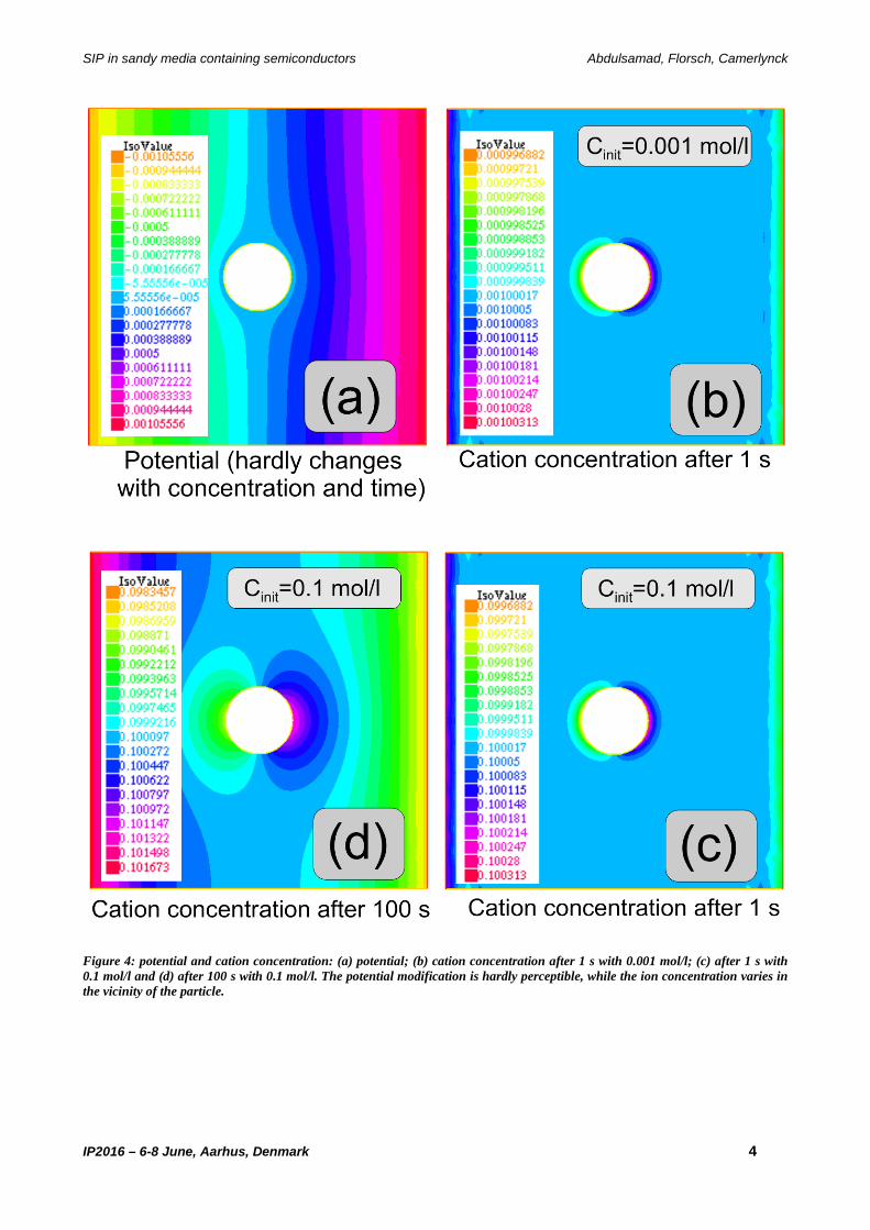
SIP in sandy media containing semiconductors Abdulsamad, Florsch, Camerlynck
IP2016 – 6-8 June, Aarhus, Denmark 4
Figure 4: potential and cation concentration: (a) potential; (b) cation concentration after 1 s with 0.001 mol/l; (c) after 1 s with 0.1 mol/l and (d) after 100 s with 0.1 mol/l. The potential modification is hardly perceptible, while the ion concentration varies in the vicinity of the particle.
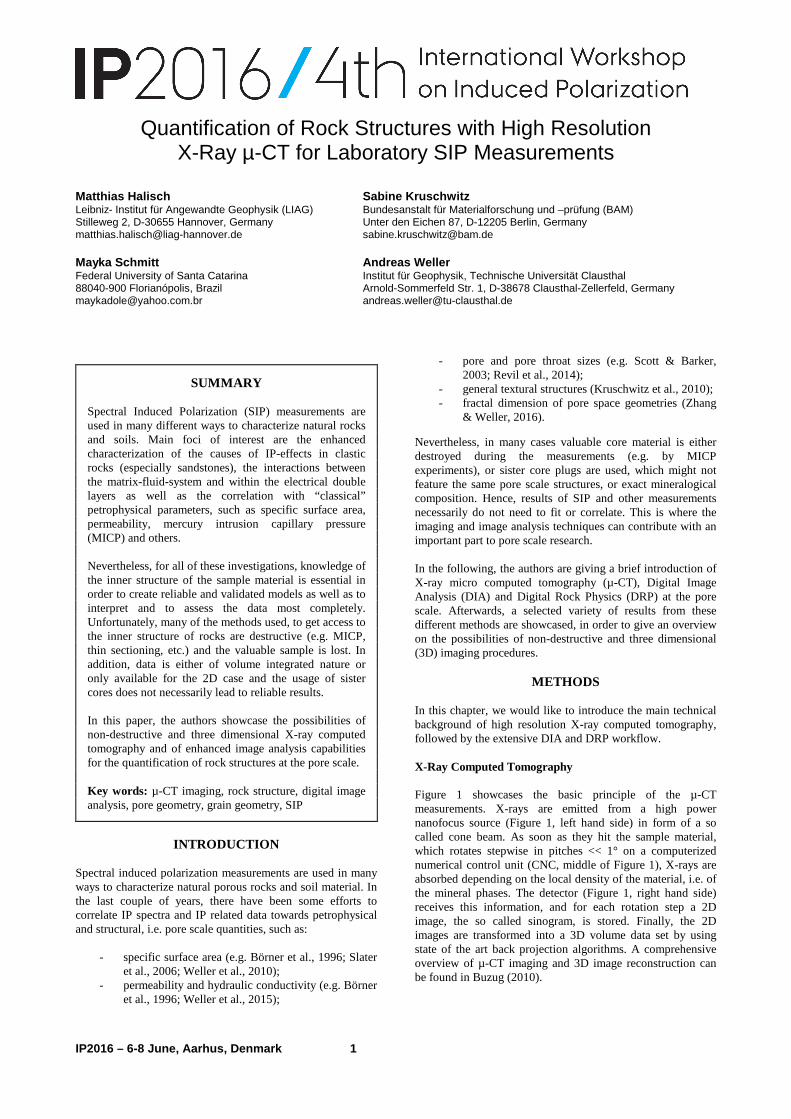
IP2016 – 6-8 June, Aarhus, Denmark 1
Quantification of Rock Structures with High Resolution X-Ray µ-CT for Laboratory SIP Measurements
Matthias Halisch Sabine Kruschwitz Leibniz- Institut für Angewandte Geophysik (LIAG) Bundesanstalt für Materialforschung und –prüfung (BAM) Stilleweg 2, D-30655 Hannover, Germany Unter den Eichen 87, D-12205 Berlin, Germany [email protected] [email protected] Mayka Schmitt Andreas Weller Federal University of Santa Catarina Institut für Geophysik, Technische Universität Clausthal 88040-900 Florianópolis, Brazil Arnold-Sommerfeld Str. 1, D-38678 Clausthal-Zellerfeld, Germany [email protected] [email protected]
INTRODUCTION
Spectral induced polarization measurements are used in many ways to characterize natural porous rocks and soil material. In the last couple of years, there have been some efforts to correlate IP spectra and IP related data towards petrophysical and structural, i.e. pore scale quantities, such as:
- specific surface area (e.g. Börner et al., 1996; Slater et al., 2006; Weller et al., 2010);
- permeability and hydraulic conductivity (e.g. Börner et al., 1996; Weller et al., 2015);
- pore and pore throat sizes (e.g. Scott & Barker, 2003; Revil et al., 2014);
- general textural structures (Kruschwitz et al., 2010); - fractal dimension of pore space geometries (Zhang
& Weller, 2016).
Nevertheless, in many cases valuable core material is either destroyed during the measurements (e.g. by MICP experiments), or sister core plugs are used, which might not feature the same pore scale structures, or exact mineralogical composition. Hence, results of SIP and other measurements necessarily do not need to fit or correlate. This is where the imaging and image analysis techniques can contribute with an important part to pore scale research. In the following, the authors are giving a brief introduction of X-ray micro computed tomography (µ-CT), Digital Image Analysis (DIA) and Digital Rock Physics (DRP) at the pore scale. Afterwards, a selected variety of results from these different methods are showcased, in order to give an overview on the possibilities of non-destructive and three dimensional (3D) imaging procedures.
METHODS In this chapter, we would like to introduce the main technical background of high resolution X-ray computed tomography, followed by the extensive DIA and DRP workflow.
X-Ray Computed Tomography Figure 1 showcases the basic principle of the µ-CT measurements. X-rays are emitted from a high power nanofocus source (Figure 1, left hand side) in form of a so called cone beam. As soon as they hit the sample material, which rotates stepwise in pitches << 1° on a computerized numerical control unit (CNC, middle of Figure 1), X-rays are absorbed depending on the local density of the material, i.e. of the mineral phases. The detector (Figure 1, right hand side) receives this information, and for each rotation step a 2D image, the so called sinogram, is stored. Finally, the 2D images are transformed into a 3D volume data set by using state of the art back projection algorithms. A comprehensive overview of µ-CT imaging and 3D image reconstruction can be found in Buzug (2010).
SUMMARY Spectral Induced Polarization (SIP) measurements are used in many different ways to characterize natural rocks and soils. Main foci of interest are the enhanced characterization of the causes of IP-effects in clastic rocks (especially sandstones), the interactions between the matrix-fluid-system and within the electrical double layers as well as the correlation with “classical” petrophysical parameters, such as specific surface area, permeability, mercury intrusion capillary pressure (MICP) and others. Nevertheless, for all of these investigations, knowledge of the inner structure of the sample material is essential in order to create reliable and validated models as well as to interpret and to assess the data most completely. Unfortunately, many of the methods used, to get access to the inner structure of rocks are destructive (e.g. MICP, thin sectioning, etc.) and the valuable sample is lost. In addition, data is either of volume integrated nature or only available for the 2D case and the usage of sister cores does not necessarily lead to reliable results. In this paper, the authors showcase the possibilities of non-destructive and three dimensional X-ray computed tomography and of enhanced image analysis capabilities for the quantification of rock structures at the pore scale. Key words: µ-CT imaging, rock structure, digital image analysis, pore geometry, grain geometry, SIP

µ-CT Rock Structure Quantification for SIP Measurements M. Halisch et al..
IP2016 – 6-8 June, Aarhus, Denmark 2
Figure 1. Basic principle of µ-CT imaging (Halisch, 2013). Digital Image Analysis & Digital Rock Physics After the sample material has been scanned by µ-CT imaging, and the data set has been reconstructed into a 3D volume file, the data should be pre-processed before the image analysis workflow starts. Pre-processing includes X-ray artefact reduction, enhanced image filtering operations (de-noising, smoothing, edge enhancement) and cropping of the data set into regions of interest (ROI) for the further investigations. Followed by these procedures, the different phases (e.g. pore space filled with air or water, main grain matrix, accessory minerals, etc) within the sample are identified and then segmented (i.e. explicitly identified and labelled). In the simplest case, pore space and minerals are segmented into two “phases” only (Figure 2).
Figure 2. Simple “two phase segmentation” of a small subsample from a Bentheimer sandstone data set, showing the detected porosity on the left and the mineral phases on the right, respectively. Depending on the specific research interest, the segmented structures can be assessed and characterized in detail by performing the DIA, allowing deriving the following (selected) parameters:
- total and effective porosity, - axial porosity distribution, - matrix mineral volume, - pore size distribution, - grain size distribution, - surface area of the grains (or pore surface), - fractal dimension, - pore shape classes, - individual pore geometry (max., min. and medium
extension), - pore and grain aspect ratios.
In addition, the processed 3D data sets can be used to perform extensive numerical modeling by using the in-situ geometries of the investigated samples. By performing DRP at the pore scale on representative volumes, the previously introduced list of parameters can be extended by the following (again, a selection):
- electrical conductivity of the rock-pore fluid-system, - formation resistivity factor, - capillary pressure at drainage and imbibition, - pore throat distribution, - permeability tensor and - diffusion coefficient.
In the following section, we would like to showcase a selection of results, focussing upon structural pore scale analyses of a small variety of sandstones.
RESULTS As explained in the previous section, different phases can be segmented for the 3D data sets. From this, the volume of the detected phase of interest can be derived (Figure 2). For the volume of the pore space, µ-CT is able to distinguish between total and effective porosity (as a function of resolution and investigated ROI), whereas most laboratory measurements are solely able to detect the effective, i.e. connected porosity. It is furthermore possible to separate the porous / grain matrix system, i.e. to disconnect the detected pores / grains from each other. By doing this, each pore / grain is labelled and gets an explicit identification number (Figure 3). From this, pore size and grain size distributions can be easily calculated.
Figure 3. Disconnecting and labelling of the pore network (left) and grain matrix (right). P1, P2, P3 indicate the three biggest pores, M1, M2 and M3 the three biggest grains, which have been identified from the ROI of Figure 2. Figure 4 displays the results from a “conventional” grain size analysis, derived by thin section analysis, and from 3D DIA. The investigated sample is a so called Baumberger sandstone, which is characterized by a fair amount of carbonatic cement, which makes the 3D analysis very challenging due to the low density contrast of the mineral phases. Nevertheless, both results indicate a remarkable good accordance and overlap. The thin section analysis slightly tends to smaller grain sizes, since not all grains are cut straight through the center, and hence edge effects are likely. In addition, DIA is able to investigate by far more grains than the 2D analysis (almost factor of 50). Nevertheless, thin section analysis features the advantage of higher resolution, so that smaller grains can be detected. Effective detection threshold for the DIA in this example is about 20 µm.

µ-CT Rock Structure Quantification for SIP Measurements M. Halisch et al..
IP2016 – 6-8 June, Aarhus, Denmark 3
Figure 4. Comparison of two different results from a grain size distribution analysis of a Baumberger sandstone sample. The greyish graph shows the results from 2D thin section analysis, the red graph shows the results from the 3D DIA. In the same way, pore size distributions can be created and assessed. Additionally, by separating the pores und labelling them individually, it is possible to characterize the equivalent 3D pore geometry, aspect ratios and pore shapes. The pore geometry is measured by using so called bounding box methods (Figure 5), which determine the x-, y- and z-length of a surrounding box for each pore individually. This can be done either by a fixed bounding box (Figure 5, left hand side), which does not consider the pore orientation, or by a so called Feret calliper box, which is oriented in direction of the largest elongation of the detected pore (Figure 5, right).
Figure 5. Different approaches to estimate the geometry of an individual pore. (a) Bounding box, (b) Feret diameter method. By using these geometries, different length ratios can be evaluated, depending on the smallest (S), medium (l) and longest (L) pore elongation (Figure 6). This leads to so called equancy and equivalent shape plots for further investigations.
Figure 6. Pore equancy (left) and shape (right) classification (Schmitt et al., 2015). Please note that the cubic / rod like shapes can be equivalently replaced with spheres or cylinders.
These results can be used to assess the pore network by individual pore (shape and equancy) clusters. Investigations from Schmitt et al. (2015) have shown that the different shape clusters can be correlated with structural pore scale features. The very cubic / spheric shapes are often linked to large pore bodies, which form the main part of the pore network. Rod or cylindrical shaped pores are often formed by altered minerals, especially by feldspars. More plate like pores are often affiliated to clayey agglomerations (e.g. clay booklets). Additionally, more general geometrical ratios can be determined, such as the average pore body – pore throat ratio, which is of interest for (e.g.) membrane polarization models, such as recently published by Bücker and Hördt (2013a & 2013b). Figure 7 showcases such a small region of interest of the main pore network of a Fontainebleau sandstone sample. The determined average ratio, i.e. pore body diameter to pore “throat” diameter is in range of 200 µm: 10 µm (20 : 1). Table 1 summarizes the results for different cretaceous sandstones. Nevertheless, it should be mentioned that these results are highly dependent of the investigated sample, due to the very high variability of structures at the pore scale.
Figure 7. Visualization of a typical pore body – pore throat – pore body system of the main pore network of a Fontainebleau sandstone. Different approaches to characterize the pore size distribution are compared in Figure 8. Besides conventional laboratory techniques like NMR or MICP, pore radii might be estimated by SIP (Niu and Revil, 2016; Zhang & Weller, 2016) and also derived by performing DRP on the 3D geometry of CT images. The main limiting factors for this kind of numerical Table 1. Pore body to pore throat ratios of main pore networks for a small selection of cretaceous sandstones: S1 = Fontainebleau, S2 = Bentheimer, S3 = Berea, S4 = Obernkirchen. avg. ratio max. ratio min. ratio
S1 20:1 25:1 10:1 S2 16:1 21:1 8:1 S3 15:1 22:1 9:1 S4 11:1 15:1 8:1
Red: 3D DIA. ~ 4900 investigated grains Grey: 2D thin section analysis. ~ 100 investigated grains
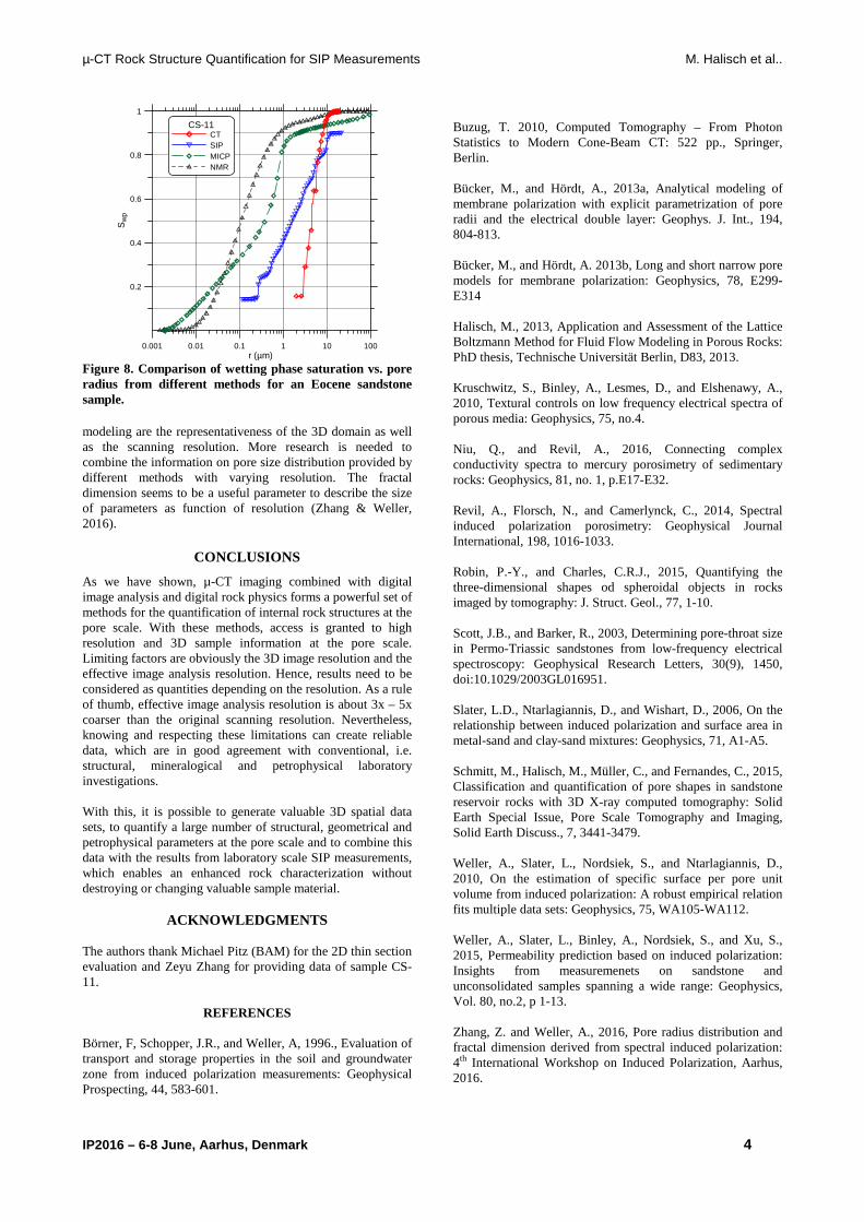
µ-CT Rock Structure Quantification for SIP Measurements M. Halisch et al..
IP2016 – 6-8 June, Aarhus, Denmark 4
0.001 0.01 0.1 1 10 100r (µm)
0.2
0.4
0.6
0.8
1S
wp
CS-11CTSIPMICPNMR
Figure 8. Comparison of wetting phase saturation vs. pore radius from different methods for an Eocene sandstone sample. modeling are the representativeness of the 3D domain as well as the scanning resolution. More research is needed to combine the information on pore size distribution provided by different methods with varying resolution. The fractal dimension seems to be a useful parameter to describe the size of parameters as function of resolution (Zhang & Weller, 2016).
CONCLUSIONS
As we have shown, µ-CT imaging combined with digital image analysis and digital rock physics forms a powerful set of methods for the quantification of internal rock structures at the pore scale. With these methods, access is granted to high resolution and 3D sample information at the pore scale. Limiting factors are obviously the 3D image resolution and the effective image analysis resolution. Hence, results need to be considered as quantities depending on the resolution. As a rule of thumb, effective image analysis resolution is about 3x – 5x coarser than the original scanning resolution. Nevertheless, knowing and respecting these limitations can create reliable data, which are in good agreement with conventional, i.e. structural, mineralogical and petrophysical laboratory investigations. With this, it is possible to generate valuable 3D spatial data sets, to quantify a large number of structural, geometrical and petrophysical parameters at the pore scale and to combine this data with the results from laboratory scale SIP measurements, which enables an enhanced rock characterization without destroying or changing valuable sample material.
ACKNOWLEDGMENTS The authors thank Michael Pitz (BAM) for the 2D thin section evaluation and Zeyu Zhang for providing data of sample CS-11.
REFERENCES Börner, F, Schopper, J.R., and Weller, A, 1996., Evaluation of transport and storage properties in the soil and groundwater zone from induced polarization measurements: Geophysical Prospecting, 44, 583-601.
Buzug, T. 2010, Computed Tomography – From Photon Statistics to Modern Cone-Beam CT: 522 pp., Springer, Berlin. Bücker, M., and Hördt, A., 2013a, Analytical modeling of membrane polarization with explicit parametrization of pore radii and the electrical double layer: Geophys. J. Int., 194, 804-813. Bücker, M., and Hördt, A. 2013b, Long and short narrow pore models for membrane polarization: Geophysics, 78, E299-E314 Halisch, M., 2013, Application and Assessment of the Lattice Boltzmann Method for Fluid Flow Modeling in Porous Rocks: PhD thesis, Technische Universität Berlin, D83, 2013. Kruschwitz, S., Binley, A., Lesmes, D., and Elshenawy, A., 2010, Textural controls on low frequency electrical spectra of porous media: Geophysics, 75, no.4. Niu, Q., and Revil, A., 2016, Connecting complex conductivity spectra to mercury porosimetry of sedimentary rocks: Geophysics, 81, no. 1, p.E17-E32. Revil, A., Florsch, N., and Camerlynck, C., 2014, Spectral induced polarization porosimetry: Geophysical Journal International, 198, 1016-1033. Robin, P.-Y., and Charles, C.R.J., 2015, Quantifying the three-dimensional shapes od spheroidal objects in rocks imaged by tomography: J. Struct. Geol., 77, 1-10. Scott, J.B., and Barker, R., 2003, Determining pore-throat size in Permo-Triassic sandstones from low-frequency electrical spectroscopy: Geophysical Research Letters, 30(9), 1450, doi:10.1029/2003GL016951. Slater, L.D., Ntarlagiannis, D., and Wishart, D., 2006, On the relationship between induced polarization and surface area in metal-sand and clay-sand mixtures: Geophysics, 71, A1-A5. Schmitt, M., Halisch, M., Müller, C., and Fernandes, C., 2015, Classification and quantification of pore shapes in sandstone reservoir rocks with 3D X-ray computed tomography: Solid Earth Special Issue, Pore Scale Tomography and Imaging, Solid Earth Discuss., 7, 3441-3479. Weller, A., Slater, L., Nordsiek, S., and Ntarlagiannis, D., 2010, On the estimation of specific surface per pore unit volume from induced polarization: A robust empirical relation fits multiple data sets: Geophysics, 75, WA105-WA112. Weller, A., Slater, L., Binley, A., Nordsiek, S., and Xu, S., 2015, Permeability prediction based on induced polarization: Insights from measuremenets on sandstone and unconsolidated samples spanning a wide range: Geophysics, Vol. 80, no.2, p 1-13. Zhang, Z. and Weller, A., 2016, Pore radius distribution and fractal dimension derived from spectral induced polarization: 4th International Workshop on Induced Polarization, Aarhus, 2016.

IP2016 – 6-8 June, Aarhus, Denmark 1
Decay-Curve Analysis for the Quantification of Data Error in Time-Domain Induced Polarization Imaging Adrián Flores Orozco Jakob Gallistl Matthias Bücker Kenneth H. Williams TU-Wien TU-Wien TU-Wien Lawrence Berkeley National Lab Vienna, Austria Vienna, Austria Vienna, Austria Berkeley, California, USA [email protected] [email protected] [email protected] [email protected]
INTRODUCTION
Initially developed for the prospection of metallic ores, the induced polarization (IP) method has emerged in recent years as a suitable technique for hydrogeological studies. As an extension of the standard DC-resistivity method, IP measurements provide information about the electrical conductivity (i.e., energy loss) and polarization (i.e., energy storage) properties of the subsurface, permitting an improved lithological characterization. Furthermore, studies using multi-frequency measurements (spectral-IP, SIP) have demonstrated the ability of the IP method to gain information about biogeochemical processes. For instances, an increase in the polarization effect has been correlated to the accumulation of bio-films in column experiments (e.g., Ntarlagiannis et al., 2005). Also, a significant increase in the polarization response has been observed due to the precipitation of metallic minerals
accompanying the stimulation of microbial activity (e.g., Williams et al., 2009; Flores Orozco et al., 2011). Furthermore, changes in the electrical signatures have been correlated to reversible chemical transformation of bio-minerals (e.g., Slater et al., 2007; Flores Orozco et al., 2013). Such results have promoted the application of the IP method in numerous investigations in the emerging discipline of biogephysics (e.g., Atekwana and Slater, 2009). Built on these findings, a recent study has explored the applicability of the IP imaging method for the prospection of naturally reduced zones (NRZ) at the floodplain scale with promising results (Wainwright et al., 2016). NRZ are spatially limited areas characterized by high rates of microbial activity and thus a disproportionally large impact on larger-scale biogeochemical cycling. Furthermore, chemical changes in the groundwater composition accompanying microbial activity in NRZ might be associated with the precipitation of metallic minerals, such as iron sulphides (FeS), which have a measurable polarization effect. Site characterization at the floodplain scale based on the analysis of soil and groundwater samples is limited by the characteristics of the samples (e.g., location of the boreholes, depth and volumes of the sampling), and often lacks the spatial resolution needed to identify NRZ. IP images provide information about the electrical properties of the floodplain sediments at a high spatial resolution and might be a suitable alternative to define NRZ. However, as pointed out by Wainwright et al. (2016), the modest polarization response of metallic biominerals places high demands on the resolution of the TDIP imaging results. An adequate characterization of data error is critical to avoid the creation of artifacts or the loss of resolution in images. Furthermore, quantitative information on data error can be used i) to remove outliers associated with systematic error and ii) for the parameterization of error models describing the characteristics of inherent random error. Flores Orozco et al. (2012) recently adopted a power-law error model to characterize the data error in IP measurements (i.e. phase or chargeability) yielding an improved resolution of the images obtained from an inversion scheme, where the data are fitted to the confidence interval defined by the error model. Furthermore, the on-site evaluation of data quality is critical to eventually improve the survey design or increase the signal-to-noise ratio (S/N). However, to date, the most widely accepted approach to evaluate IP data quality is based on the analysis of the misfit between normal and reciprocal measurements, where reciprocal measurements are those collected with interchanged current and potential electrodes. Though, the necessity to reduce the acquisition time for large-scale surveys compromises the collection of reciprocals.
SUMMARY Recent studies have demonstrated the advantages of a careful processing of induced polarization (IP) imaging datasets. In particular, inversion results based on an adequate quantification of data error provide IP images with enhanced contrasts and a better correlation with subsurface structures and processes. The analysis of the discrepancy between normal and reciprocal readings is a widely accepted measure to assess quality of imaging datasets and parametrize error models. However, the collection of reciprocal measurements increases acquisition time and is not always feasible. Therefore, we propose an alternative methodology to quantify data error of time-domain IP (TDIP) imaging measurements based on the analysis of the recorded IP decay curve. Our approach provides detailed information about data error as required for the identification of outliers and the quantification of error parameters without the need of reciprocal measurements. Comparison of the error parameters and imaging results following our proposed decay-curve analysis (DCA) and the conventional normal-reciprocal analysis revealed consistent results, demonstrating the accuracy of our approach. We illustrate the practical applicability of our approach with the inversion results for an extensive field data set collected at the floodplain scale aiming at the localization of so-called “biogeochemical hot-spots”, which are areas characterized by high rates of microbial activity and the accumulation of iron sulphides. Key words: data processing, error quantification, time-domain IP, hydrogeophysics, biogeophysics.

Decay Curve Analysis in TDIP imaging A. Flores Orozco, J. Gallistl, M. Bücker, and K. H. Williams
IP2016 – 6-8 June, Aarhus, Denmark 2
Furthermore, measuring configurations characterized by high S/N, such as the multiple-gradient array (Dahlin and Zhou, 2006), are not suited for the collection of reciprocals with multi-channel instruments without drastically increasing the acquisition time. Accordingly, IP surveys at the large scale call for the development of new techniques to quickly and though reliably quantify data quality without the need of reciprocal readings. Here, we propose a new methodology to quantify data-error parameters based on the analysis of the voltage decay of time-domain IP (TDIP) measurements. Inversion of TDIP measurements were performed using error parameters obtained after the analysis of normal-reciprocal misfit (NRM) and with the proposed decay curve analysis (DCA) to evaluate the performance of the proposed algorithm. We demonstrate the applicability of the new approach with an extensive TDIP data set collected at the floodplain scale that includes dipole-dipole and multiple-gradient data. The objective of the IP survey was the identification of possible NRZ.
STUDY AREA AND SETTINGS
Figure 1. Layout of the TDIP profiles (red lines) collected at the Shiprock site. Measurements were collected at the Shiprock Site (New Mexico, USA) on the grounds of a former uranium-processing facility. The site has been remediated but remanent concentrations of uranium are still observed in water samples. The site’s stratigraphy is characterized by three main units: an impermeable clay-rich layer extending from the surface to ~2 m depth, followed by a sandy-gravel aquifer (~3 m thickness) on top of the low permeable Macos Shale. Groundwater level was located at a depth ~3m during the field surveys. Studies on similar sites (Wainwright et al., 2016) revealed that fluvially deposited organic material within aquifer sediments naturally stimulates the activity of subsurface microorganisms leading to both the natural immobilization of uranium and the accumulation of reduced end products (minerals and pore
fluids). In order to map these possible hot spots, which are expected to generate measureable IP anomalies, a total of 22 IP profiles were collected. Six long profiles (up to 350 m) helped to fairly characterize large-scale changes in the electrical properties along the floodplain, and 16 shorter profiles were used to improve the resolution of particular areas of interest (Figure 1). TDIP measurements were collected using the Syscal Iris Pro 72 Switch equipment with a square-wave current injection, 50% duty cycle, and a pulse length of two seconds. The voltage decay was measured along 20 windows between 240 and 1840 milliseconds (ms) after current shut-off. All measurements were collected using a separation of 2 m between electrodes and two configurations: 1) Dipole-Dipole (DD) skip-2 and skip-3 (i.e., a length of 6 and 8 m for both current and potential dipoles), and 2) multiple-gradient (MG) configurations (after Dahlin and Zhou, 2006) with 10 potential dipoles (ski-0, skip-1 and skip-2) nested within the current dipole. DD measurements were collected as normal-reciprocal pairs. In order to reduce acquisition time, the depth of investigation was limited to 7 m, which allowed defining the bottom of the aquifer at the upper limit of the Mancos Shale. The data error in DD measurements was quantified using the bin analysis for the normal-reciprocal misfit and error-models described in Flores Orozco et al. (2012). All data was inverted with CRTomo an algorithm by Kemna (2000), which permits the inversion of the data only to the confidence level determined by the error model. For inversions with CRTomo, chargeability values were linearly converted to frequency-domain phase values (at the fundamental frequency of 0.125 Hz) assuming a constant-phase response (Kemna, 1997).
DECAY-CURVE ANALYSIS Initial inversion of MG measurements using error parameters of co-located DD datasets resulted in images that were affected by artifacts (not shown here) due to the over estimation of data error. As expected, a more detailed analysis of the decay curves (see Figure 2) revealed smooth curves for measurements associated with high S/N (i.e., low geometrical factors) and increasingly distorted curves for measurements collected with larger separations between the potential and current electrodes (lower S/N, higher geometrical factors). Previous studies reported similar observations and proposed to manually remove measurements associated with an erratic (or increasing) behaviour of the decay curves (e.g., Gazoty et al., 2013; Doetch et al., 2015).
Figure 2. Measured decay curves with DD configurations (red symbols) for small (left), medium (centre) and maximum (right) separation between current and potential dipoles (i.e., S/N). The negative power law model fitted to each curve is indicated with the blue line.
N

Decay Curve Analysis in TDIP imaging A. Flores Orozco, J. Gallistl, M. Bücker, and K. H. Williams
IP2016 – 6-8 June, Aarhus, Denmark 3
The first step of our processing consists in fitting a negative power-law model (fitted decay curve, FDC) to each measured decay curve (MDC). Such model yields a good fit of most decays while involving a minimum number of parameters. All physically meaningful MDC should be positive and decrease with time. Hence, a first filter removes all measurements associated with non-decaying curves, while measurements associated with an erratic behaviour were not removed. At this point, the actual goodness of the fit is not used for filtering, as this would remove erratic decay curves, typically related to larger separations between electrodes, i.e., “deeper” information, which is critical to solve for accurate images at depth. To explore the robustness of the FDC, we performed a series of analysis. For instances, we compared power-law fits to smaller subsets of the decay curve (odd and even IP windows) or using other models than the proposed power-law fit. Nevertheless, all results were consistent to those using the negative power-law model. To further evaluate the accuracy of the FDC we compared the integral chargeability obtained from the MDC and the FDC, which we found to be very consistent (Figure 3).
Figure 3. Comparison of the integral chargeability values computed from measured (MDC) and fitted (FDC) decay curves. To this point each FDC has been fitted independently, which might still result in a high spatial variability of the fitted models. However, due to the nature of the tomographic measurements, chargeabilities are expected to vary in a relatively smooth manner. Therefore, the second step of our analysis assesses the spatial consistency of all FDC of a tomographic dataset to identify and remove outliers. To this end, we compute a master decay curve as the median value of all measurements, and then adjust its position along the y-axis (i.e., the magnitude of the voltage values) to each individual MDC. The resulting curve, i.e. the shifted master decay curve, defines an improved FDC for each measurement. Outliers are then defined as those measurements associated with a large discrepancy between the MDC and the master decay curve. The filtered DD pseudosections in Figure 4 show that both NRA- and DCA-based filters consistently remove most outliers. Yet, the DCA filter removes fewer measurements associated with relatively high integral chargeabilities and/or small separations between electrodes. This illustrates the main difference between the two approaches. While the DCA only evaluates the similarity of all MDC in a data set with the shape of the master decay curve, the NRA is sensible to variations of the offset of the decay curves, the magnitude of which is higher at small dipole spacings and large chargeabilities.
Figure 4. Pseudosection for DD measurements after the removal of outliers as defined by the proposed DCA (top) and standard NRA (bottom). In a third step, we compute the discrepancy between the MDC and the FDC (fitted in step one), based on the individual misfits for each IP window. This approach allows us to quantify the temporal instability (i.e. erratic behaviour) of the measured signal and use this information to quantify the data error (i.e. standard deviation of a measurement). If we used the misfit of the integral chargeabilities instead, the obtained error would not properly assess the quality of the decay curve. Furthermore, later IP windows are associated with lower voltage values (i.e., lower S/N), thus the analysis of the misfit for each independent window permits a detailed analysis for a larger dynamic in the signal strength. The misfit between FDC and MDC can be used in a similar way as the misfit between normal and reciprocal readings to describe the error of the integral chargeability of a dataset. Figure 5 shows the FDC-MDC misfits and the normal-reciprocal misfit of the same DD data set, both in function of the respective transfer resistances. The patterns of the misfits of DCA and NRA are consistent and exhibit similar power-law distributions.
Figure 5. Chargeability error estimates based on DCA- and NRA-misfits plotted as a function of the transfer resistances. Subsequently, error parameters were obtained for datasets processed by NRA and DCA following the methodology described in Flores Orozco et al. (2012b). Figure 6 presents a comparison of the imaging results for the polarization effect expressed in terms of the phase shift of the complex electrical resistivity. Images of the magnitude of the complex electrical resistivity revealed no significant changes between the two approaches (not shown here). Both phase images consistently resolved the main geological units; the low phase values correspond to the unsaturated clay-rich top layer and the low permeable Mancos clay at the bottom, whereas the high phase values are associated with the sandy-gravel aquifer material. Nevertheless, it is obvious that the NRA was not accurate enough to detect outliers in the datasets solving for the less-

Decay Curve Analysis in TDIP imaging A. Flores Orozco, J. Gallistl, M. Bücker, and K. H. Williams
IP2016 – 6-8 June, Aarhus, Denmark 4
polarizable anomaly located at ~90 m along profile. The enhanced resolution and the lack of artifacts clearly demonstrate the applicability of and the additional benefit provided by the proposed DCA.
Figure 6. IP imaging results in terms of the phase of the complex electrical resistivity for data processed after the proposed DCA and standard NRA. After performing the DCA and inversion of the entire dataset, it was possible to construct maps representing the electrical properties of the subsurface at different depths. Figure 7 presents the inverted phase values for aquifer materials (at a depth of 4.5 m), which reveal clear anomalies characterized by high IP values (>10 mrad). Ongoing work consists on the collection of aquifer materials to confirm the presence of NRZ in areas associated to high IP response
Figure 7. Map of the Shiprock Site presenting the distribution of phase values in aquifer materials (at a depth of 4.5 m).
CONCLUSIONS We propose a new methodology for the processing of TDIP imaging data sets based on the analysis of the IP decay curve. Our approach reliably identifies outliers and provides an adequate quantification of the data error. Error parameters obtained with the proposed DCA and standard NRA are consistent, which clearly demonstrates the applicability of our approach. Imaging results obtained with the DCA resulted in images with enhanced contrasts and less artefacts compared to
those images obtained with the NRA. Based on our results, the new approach is able to improve the quality of IP images.
REFERENCES Atekwana, E.A., and Slater, L.D., 2009, Biogeophysics: A new frontier in Earth science research: Reviews of Geophysics 47, RG4004. Dahlin, T., Zhou, B.,. 2006, Multiple-gradient array measurements for multichannel 2D resistivity imaging: Near Surface Geophysics 4(2), 113-123. Doetsch, J., Ingeman-Nielsen, T., Christiansen, A. V., Fiandaca, G., Auken, E., and Elberling, B., 2015, Direct current (DC) resistivity and induced polarization (IP) monitoring of active layer dynamics at high temporal resolution: Cold Regions Science and Technology, 119, 16-28. Flores Orozco, A., Kemna, A., Zimmermann, E.,. 2012, Data error quantification in spectral induced polarization imaging: Geophysics 77(3), E227-E237. Flores Orozco, A., Williams, K.H., Long, P.E., Hubbard, S. S., Kemna, A.,. 2011, Using complex resistivity imaging to infer biogeochemical processes associated with bioremediation of an uranium-contaminated aquifer: Journal of Geophysical Research: Biogeosciences 116(G3), 2156-2206. Flores Orozco, A., Williams, K.H., Kemna, A.,. 2013, Time-lapse spectral induced polarization imaging of stimulated uranium bioremediation: Near Surface Geophysics: 11(5), 531-544. Gazoty, A., Fiandaca, G., Pedersen, J., Auken, E., & Christiansen, A. V., 2013, Data repeatability and acquisition techniques for time-domain spectral induced polarization: Near Surface Geophysics, 11(4), 391-406. Kemna, A., 2000. Tomographic Inversion of Complex Resistivity: Theory and Application, Der Andere Verlag, Osnabrück. Ntarlagiannis, D., Yee, N., and Slater, L., 2005, On the low-frequency electrical polarization of bacterial cells in sands: Geophysical Research Letters 32, L24402. Slater, L., Ntarlagiannis, D., Personna, Y.R., and Hubbard, S., 2007, Pore-scale spectral induced polarization signatures associated with FeS biomineral transformations: Geophysical Research Letters 34. Wainwright, H. M., Flores Orozco, A.., Bücker, M., Dafflon, B., Chen, J., Hubbard, S. S., and Williams, K. H., 2015, Hierarchical Bayesian method for mapping biogeochemical hot spots using induced polarization imaging. Water Resources Research 52, 533-551. Williams, K.H., Kemna, A., Wilkins, M.J., Druhan, J., Arntzen, E., N'Guessan, A.L., Long, P.E., Hubbard, S.S., and Banfield, J.F., 2009, Geophysical monitoring of coupled microbial and geochemical processes during stimulated subsurface bioremediation: Environmental Science and Technology 43, 6717-6723.
N
IP2016 – 6-8 June, Aarhus, Denmark 1
Advances in spectral inversion of time-domain induced polarization Gianluca Fiandaca Esben Auken Anders Vest Christiansen
HydroGeophysics Group HydroGeophysics Group HydroGeophysics Group Department of Geoscience Department of Geoscience Department of Geoscience Aarhus University (Denmark) Aarhus University (Denmark) Aarhus University (Denmark) [email protected] [email protected] [email protected]
INTRODUCTION
Recently, the interpretation and inversion of TDIP data has
changed from only inverting for the integral changeability to
consider also the spectral information contained in the IP
response curves (Fiandaca et al., 2012, 2013). Several
examples of spectral TDIP applications have been presented,
for landfill delineation (Gazoty et al., 2012b, 2013; Wemegah
et al., 2016), lithotype characterization (Chongo et al., 2015;
Gazoty et al., 2012a; Johansson et al., 2015, 2016; Maurya et
al., 2016), time-lapse monitoring of CO2 injection (Doetsch et
al., 2015a) and freezing of active layer in permafrost (Doetsch
et al., 2015b). Furthermore, efforts have been made to achieve
a wider time-range in TDIP acquisition, up to four decades in
time (Olsson et al., 2016), for enhanced spectral content. In
this work a review of the recent advances in spectral inversion
of TDIP data is presented, in terms of: supported IP
parameterizations; modelling of transmitter waveform; support
for buried electrodes; model regularization; computation of the
depth of investigation.
ADVANCES IN SPECTRAL TDIP INVERSION
In the spectral inversion of TDIP data, the data space is
composed by the apparent resistivity and the full voltage
decays, while the model space is constituted by a
parameterization of IP. The Cole-Cole model (Cole-Cole,
1941; Pelton et al., 1978) and the Constant Phase Angle
(CPA) model (Van Voorhis et al., 1973) are the two
parameterizations currently implemented in AarhusInv (Auken
et al., 2015), the software in which the inversion algorithms
described in Fiandaca et al. (2012,2013) are implemented. The
complex resistivity ζCole-Cole of the Cole-Cole model takes the
form:
𝜁𝐶𝑜𝑙𝑒−𝐶𝑜𝑙𝑒 = 𝜌 (1 − 𝑚0 (1 −1
1 + (𝑖𝜔𝜏)𝐶))
(1)
where ρ is the direct current resistivity, m0 is the intrinsic
chargeability, τ is the time constant, C is the frequency
exponent and i is the imaginary unit. The complex resistivity
𝜁𝐶𝑃𝐴 of CPA model is expressed as:
𝜁𝐶𝑃𝐴 = 𝐾(𝑖𝜔)−𝑏 (2)
where b is a positive fraction, 𝜑 = −𝜋
2𝑏 represents the phase
shift and defines completely the IP response, K is a constant
and i is the imaginary unit. In the CPA model, the DC
resistivity cannot be defined, because the complex resistivity
increases indefinitely at low frequencies. For this reason, Van
Voorhis et al. (1973) introduced the Drake model:
𝜁𝐷𝑟𝑎𝑘𝑒 = 𝐾(𝑖𝜔 + 𝜔𝐿)−𝑏 (3)
where in comparison with the CPA model a low frequency
pole 𝜔𝐿 is introduced and the DC resistivity can be defined as
𝜌 = 𝐾𝜔𝐿−𝑏. In the AarhusInv implementation of the time-
domain CPA forward response the Drake model of equation
(3) is actually used, with a fixed value for the low frequency
pole 𝜔𝐿 = 10−5 Hz. In this way, the CPA inversion is set up
in terms of the model parameters 𝜌 and 𝜑, while the Cole-
Cole inversion is set up in terms of ρ, m0, τ and C. Considering
that the CPA and the Cole-Cole models are easily
distinguishable in time-domain when more than 2 orders of
magnitudes are acquired in the time-range (Lajaunie et al.,
2016), the choice between the different supported IP
parameterizations can be driven by the actual spectral content
of the data. For both models it is also possible to invert
directly for the normalized chargeability parameters 𝜑/𝜌 or
𝑚0/𝜌, instead of 𝜑 or 𝑚0.
The forward modelling in AarhusInv, whatever
parameterization is used for IP, takes into account the
transmitter waveform and the receiver transfer function
(Figure 1), for an accurate modelling of the IP response
(Fiandaca et al., 2012,2013). The inversion is performed
iteratively, by using the first term of the Taylor expansion of
the nonlinear forward mapping of the model to the data space,
as described in details in Auken et al. (2015). Figure 2 shows
two typical forward responses for Cole-Cole and CPA
homogeneous half spaces. The shape of the decays contains
the spectral information of the IP phenomenon, which can be
properly retrieved when the transmitter/receiver characteristics
are properly modelled (Fiandaca et al., 2012; Fiandaca et al.,
2013; Lajaunie et al., 2016; Madsen et al., 2016). Recently,
the modelling of the IP response during the current on-time
with a 100% duty cycle transmitter waveform has been
implemented in AarhusInv (Figure 3). With the 100% duty
cycle the current switches directly from positive to negative
values, allowing for shorter acquisition times (because the off-
time is skipped) and better signal-to-noise ratio (because the
measured voltages are higher for the 100% duty cycle), but
keeping equivalent spectral content when compared to the
SUMMARY The extraction of spectral information in the inversion
process of time-domain (TD) induced polarization (IP)
data is changing the use of the TDIP method. Data
interpretation is evolving from a qualitative description of
the subsurface, able only to discriminate the presence of
contrasts in chargeability parameters, towards a
quantitative analysis of the investigated media, which
allows for detailed soil- and rock-type characterization. In
this work a review of the recent advances in spectral
inversion of TDIP data is presented, in terms of:
supported IP parameterizations; modelling of transmitter
waveform; support for buried electrodes; model
regularization; computation of the depth of investigation.
Keywords: spectral inversion, time-domain, Cole-Cole,
CPA, transmitter waveform

Advances in spectral inversion of TDIP Fiandaca et al.
MRS2015 – 8-10 June, Aarhus, Denmark 2
50% duty cycle waveform (Olsson et al., 2015; Madsen et al.,
2016).
Figure 1 (after Fiandaca et al, 2013). (a) Construction of
the actual response by superimposing step responses; (b)
IP percentage difference between decays with different
number of stacks (a decay stacked six times is used as a
reference) for the homogeneous half-space described by
the Cole–Cole parameters (m0 = 100 mV/V, τ =2 s, C=0.5).
(c) IRIS Syscal Pro filter effect (circles) measured in the
time domain on a non-chargeable resistor. (d) Example of
forward response with the filter implementation (black
line) and without the filter implementation (grey line).
Figure 2. Examples of Cole-Cole decay (red curve) and
CPA decay (blue curve) for homogeneous half spaces and
50% duty cycle waveform (Ton= Toff =10 s, 4 stacked
pulses).
In addition to the 1-D and 2-D implementations described in
Fiandaca et al. (2012,2013), the IP forward modelling in
AarhusInv has been recently enriched by the possibility of
computing the response for buried electrodes, for inversion of
1-D borehole and 2-D cross-borehole data. The 1-D
implementation computes the kernel following Sato (2000),
with recursion formulas over the layers. Considering that in
borehole data often hundreds of layers are modelled (Auken et
al., 2016), the lateral-constrained approach has been
implemented for speeding-up computations. The full 1-D
model containing hundreds of layers is split into several sub-
models containing only a few tens of layers and the data are
subdivided in subsets grouped by pseudodepth.
Figure 3. 50% duty cycle decays (circles) and 100% duty
cycle decays (triangles) for Cole-Cole homogeneous
halfspace (ρ=100 Ωm, m0=40 mV/V, τ=0.01 s, C=0.3,
Ton/Toff =10 s, 4 stacked pulses). Black lines represent the
normalized decays in mV/V, while red lines represent the
actual voltages (see Olsson et al. (2015) for details).
Figure 4. Split of a 32-layers 1D model (grey model) in six
13-layers laterally-constrained sub-models for
computational efficiency. The red arrows represent the
lateral constraints.
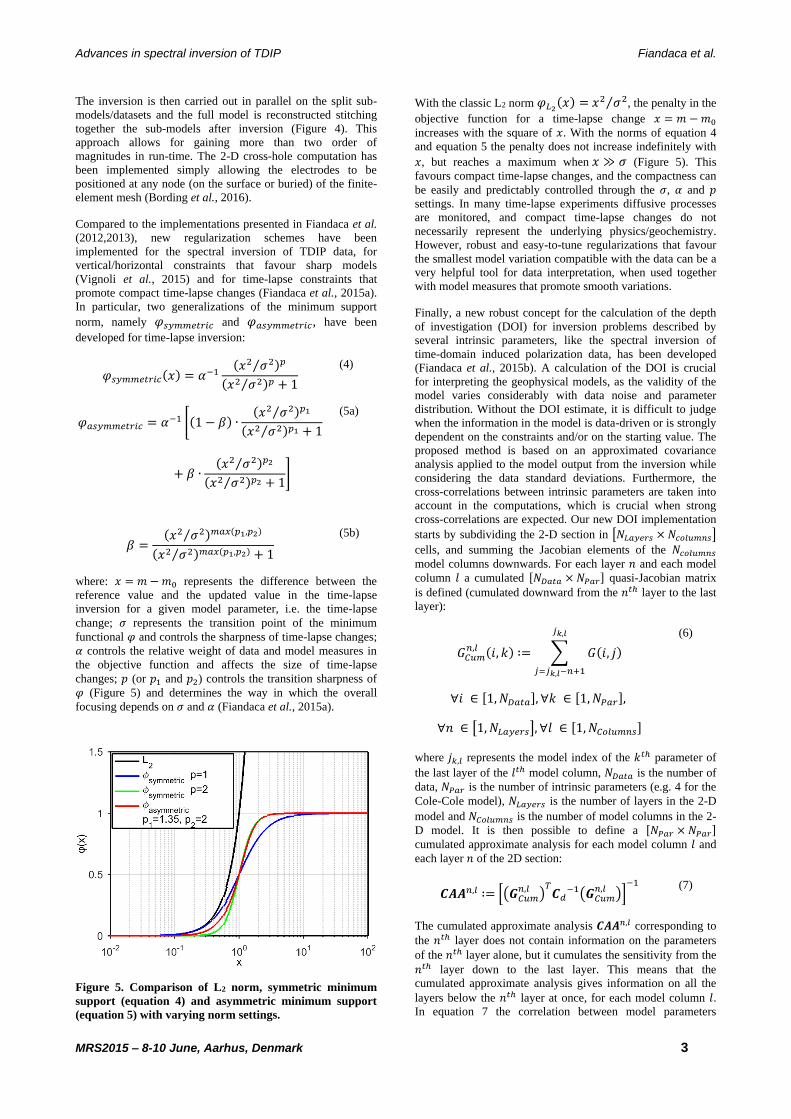
Advances in spectral inversion of TDIP Fiandaca et al.
MRS2015 – 8-10 June, Aarhus, Denmark 3
The inversion is then carried out in parallel on the split sub-
models/datasets and the full model is reconstructed stitching
together the sub-models after inversion (Figure 4). This
approach allows for gaining more than two order of
magnitudes in run-time. The 2-D cross-hole computation has
been implemented simply allowing the electrodes to be
positioned at any node (on the surface or buried) of the finite-
element mesh (Bording et al., 2016).
Compared to the implementations presented in Fiandaca et al.
(2012,2013), new regularization schemes have been
implemented for the spectral inversion of TDIP data, for
vertical/horizontal constraints that favour sharp models
(Vignoli et al., 2015) and for time-lapse constraints that
promote compact time-lapse changes (Fiandaca et al., 2015a).
In particular, two generalizations of the minimum support
norm, namely 𝜑𝑠𝑦𝑚𝑚𝑒𝑡𝑟𝑖𝑐 and 𝜑𝑎𝑠𝑦𝑚𝑚𝑒𝑡𝑟𝑖𝑐, have been
developed for time-lapse inversion:
𝜑𝑠𝑦𝑚𝑚𝑒𝑡𝑟𝑖𝑐(𝑥) = 𝛼−1(𝑥2 𝜎2⁄ )𝑝
(𝑥2 𝜎2⁄ )𝑝 + 1
(4)
𝜑𝑎𝑠𝑦𝑚𝑚𝑒𝑡𝑟𝑖𝑐 = 𝛼−1 [(1 − 𝛽) ∙(𝑥2 𝜎2⁄ )𝑝1
(𝑥2 𝜎2⁄ )𝑝1 + 1
+ 𝛽 ∙(𝑥2 𝜎2⁄ )𝑝2
(𝑥2 𝜎2⁄ )𝑝2 + 1]
(5a)
𝛽 =(𝑥2 𝜎2⁄ )𝑚𝑎𝑥(𝑝1,𝑝2)
(𝑥2 𝜎2⁄ )𝑚𝑎𝑥(𝑝1,𝑝2) + 1
(5b)
where: 𝑥 = 𝑚 − 𝑚0 represents the difference between the
reference value and the updated value in the time-lapse
inversion for a given model parameter, i.e. the time-lapse
change; 𝜎 represents the transition point of the minimum
functional 𝜑 and controls the sharpness of time-lapse changes;
𝛼 controls the relative weight of data and model measures in
the objective function and affects the size of time-lapse
changes; 𝑝 (or 𝑝1 and 𝑝2) controls the transition sharpness of
𝜑 (Figure 5) and determines the way in which the overall
focusing depends on 𝜎 and 𝛼 (Fiandaca et al., 2015a).
Figure 5. Comparison of L2 norm, symmetric minimum
support (equation 4) and asymmetric minimum support
(equation 5) with varying norm settings.
With the classic L2 norm 𝜑𝐿2(𝑥) = 𝑥2 𝜎2⁄ , the penalty in the
objective function for a time-lapse change 𝑥 = 𝑚 − 𝑚0
increases with the square of 𝑥. With the norms of equation 4
and equation 5 the penalty does not increase indefinitely with
𝑥, but reaches a maximum when 𝑥 ≫ 𝜎 (Figure 5). This
favours compact time-lapse changes, and the compactness can
be easily and predictably controlled through the 𝜎, 𝛼 and 𝑝
settings. In many time-lapse experiments diffusive processes
are monitored, and compact time-lapse changes do not
necessarily represent the underlying physics/geochemistry.
However, robust and easy-to-tune regularizations that favour
the smallest model variation compatible with the data can be a
very helpful tool for data interpretation, when used together
with model measures that promote smooth variations.
Finally, a new robust concept for the calculation of the depth
of investigation (DOI) for inversion problems described by
several intrinsic parameters, like the spectral inversion of
time-domain induced polarization data, has been developed
(Fiandaca et al., 2015b). A calculation of the DOI is crucial
for interpreting the geophysical models, as the validity of the
model varies considerably with data noise and parameter
distribution. Without the DOI estimate, it is difficult to judge
when the information in the model is data-driven or is strongly
dependent on the constraints and/or on the starting value. The
proposed method is based on an approximated covariance
analysis applied to the model output from the inversion while
considering the data standard deviations. Furthermore, the
cross-correlations between intrinsic parameters are taken into
account in the computations, which is crucial when strong
cross-correlations are expected. Our new DOI implementation
starts by subdividing the 2-D section in [𝑁𝐿𝑎𝑦𝑒𝑟𝑠 × 𝑁𝑐𝑜𝑙𝑢𝑚𝑛𝑠]
cells, and summing the Jacobian elements of the 𝑁𝑐𝑜𝑙𝑢𝑚𝑛𝑠
model columns downwards. For each layer 𝑛 and each model
column 𝑙 a cumulated [𝑁𝐷𝑎𝑡𝑎 × 𝑁𝑃𝑎𝑟] quasi-Jacobian matrix
is defined (cumulated downward from the 𝑛𝑡ℎ layer to the last
layer):
𝐺𝐶𝑢𝑚𝑛,𝑙 (𝑖, 𝑘) ∶= ∑ 𝐺(𝑖, 𝑗)
𝑗𝑘,𝑙
𝑗=𝑗𝑘,𝑙−𝑛+1
∀𝑖 ∈ [1, 𝑁𝐷𝑎𝑡𝑎], ∀𝑘 ∈ [1, 𝑁𝑃𝑎𝑟],
∀𝑛 ∈ [1, 𝑁𝐿𝑎𝑦𝑒𝑟𝑠], ∀𝑙 ∈ [1, 𝑁𝐶𝑜𝑙𝑢𝑚𝑛𝑠]
(6)
where 𝑗𝑘,𝑙 represents the model index of the 𝑘𝑡ℎ parameter of
the last layer of the 𝑙𝑡ℎ model column, 𝑁𝐷𝑎𝑡𝑎 is the number of
data, 𝑁𝑃𝑎𝑟 is the number of intrinsic parameters (e.g. 4 for the
Cole-Cole model), 𝑁𝐿𝑎𝑦𝑒𝑟𝑠 is the number of layers in the 2-D
model and 𝑁𝐶𝑜𝑙𝑢𝑚𝑛𝑠 is the number of model columns in the 2-
D model. It is then possible to define a [𝑁𝑃𝑎𝑟 × 𝑁𝑃𝑎𝑟] cumulated approximate analysis for each model column 𝑙 and
each layer 𝑛 of the 2D section:
𝑪𝑨𝑨𝑛,𝑙 ∶= [(𝑮𝐶𝑢𝑚𝑛,𝑙 )
𝑇𝑪𝑑
−1(𝑮𝐶𝑢𝑚𝑛,𝑙 )]
−1
(7)
The cumulated approximate analysis 𝑪𝑨𝑨𝑛,𝑙 corresponding to
the 𝑛𝑡ℎ layer does not contain information on the parameters
of the 𝑛𝑡ℎ layer alone, but it cumulates the sensitivity from the
𝑛𝑡ℎ layer down to the last layer. This means that the
cumulated approximate analysis gives information on all the
layers below the 𝑛𝑡ℎ layer at once, for each model column 𝑙. In equation 7 the correlation between model parameters

Advances in spectral inversion of TDIP Fiandaca et al.
MRS2015 – 8-10 June, Aarhus, Denmark 4
belonging to different model columns are neglected (lateral
data correlation), but the correlation among the 𝑁𝑃𝑎𝑟 intrinsic
parameters for each model column is considered. The
inversion is carried out in logarithmic model space, and thus
we use a standard deviation factor, 𝑆𝑇𝐷𝐹, for each parameter
𝑘:
𝑆𝑇𝐷𝐹𝑛,𝑙(𝑘) ∶= 𝑒𝑥𝑝 (√𝐶𝐴𝐴𝑛,𝑙(𝑘, 𝑘)) (8)
The DOI-value is then defined for each parameter 𝑘 and each
model column 𝑙 by imposing a threshold value for the 𝑆𝑇𝐷𝐹,
bearing the implicit meaning that below this threshold the
model structures are not data driven, but rather a result of the
constraints and/or inversion properties. Figure 6 shows the
𝑆𝑇𝐷𝐹 values and the corresponding DOI computations for a
typical 3-layers Cole-Cole model for a Schlumberger sounding
(red lines). Furthermore, the results when disregarding the off-
diagonal elements in (𝑮𝐶𝑢𝑚𝑛,𝑙 )
𝑇𝑪𝑑
−1(𝑮𝐶𝑢𝑚𝑛,𝑙 ), i.e. the
parameter correlations, are presented (blue lines): the DOI is
significantly overestimated when neglecting the parameter
correlations.
Figure 6. Depth of investigation (DOI) for an exemplary 3-layers Cole-Cole model for a Schlumberger sounding. Black
dashed lines: layer interfaces. Continuous grey lines: vertical model subdivision for the 𝑺𝑻𝑫𝑭 computation (equation 8) as a
function of depth. Green dashed lines: threshold value for the 𝑺𝑻𝑫𝑭 computation. Red lines: 𝑺𝑻𝑫𝑭 values as a function of
depth taking into account the parameter correlations (continuous lines) and corresponding DOI values (dashed lines). Blue
lines: 𝑺𝑻𝑫𝑭 values as a function of depth disregarding the parameter correlations (continuous lines) and corresponding
overestimated DOI values (dashed lines).
CONCLUSIONS
The spectral inversion of TDIP data has reached maturity.
Different IP parameterizations can be modelled, i.e. the Cole-
Cole and the CPA models, and the choice between the models
can be made in function of the actual spectral content of the
data. The forward modelling takes into account the transmitter
waveform and the receiver transfer function for accurate
computations, and the 100% duty cycle is supported for
shorted acquisition time and better signal-to-noise ratio.
Computation with buried electrodes for 1-D and 2-D
modelling has been implemented, and advanced model
regularizations have been developed, for sharp
vertical/horizontal model variations and compact changes in
time-lapse inversion. Furthermore, a new robust concept for
the calculation of the depth of investigation has been
developed, enabling judging when the information in the
model is data-driven or is strongly dependent on the
constraints and/or on the starting value. We believe that the
advances in spectral TDIP inversion significantly increase the
potential of TDIP in (hydro)geophysical applications.
ACKNOWLEDGMENTS
Support was provided by the research project GEOCON,
Advancing GEOlogical, geophysical and CONtaminant
monitoring technologies for contaminated site investigation
(contract 1305-00004B). The funding for GEOCON is
provided by The Danish Council for Strategic Research under
the Programme commission on sustainable energy and
environment.
REFERENCES Auken E., Christiansen A.V., Kirkegaard C., Fiandaca G.,
Schamper C., Behroozmand A.A., Binley A., Nielsen E.,
Efferso F., Christensen N.B., Sorensen K., Foged N. &
Vignoli G., 2015. An overview of a highly versatile forward
and stable inverse algorithm for airborne, ground-based and
borehole electromagnetic and electric data, Exploration
Geophysics, 46, 223-235. 10.1071/eg13097.

Advances in spectral inversion of TDIP Fiandaca et al.
MRS2015 – 8-10 June, Aarhus, Denmark 5
Auken E., Fiandaca G., Christiansen A.V., Maurya P.K.,
Holm H., 2016. Mapping lithotypes using in-situ measurement
of time domain induced polarization: El-log. 4th IP Workshop,
6-8 June 2016, Aarhus, Denmark.
Bording T.S., Fiandaca G., Maurya P.K., Auken E.,
Christiansen A.V., 2016. Mapping possible flowpaths of
contaminants through surface and cross-borehole spectral
time-domain induced polarization. 4th IP Workshop, 6-8 June
2016, Aarhus, Denmark.
Chongo M., Christiansen A.V., Fiandaca G., Nyambe I.A.,
Larsen F. & Bauer-Gottwein P., 2015. Mapping localised
freshwater anomalies in the brackish paleo-lake sediments of
the Machile-Zambezi Basin with transient electromagnetic
sounding, geoelectrical imaging and induced polarisation,
Journal of Applied Geophysics, 123, 81-92.
10.1016/j.jappgeo.2015.10.002.
Cole K.S., Cole R.H., 1941. Dispersion and absorption in
dielectrics I. Alternating current characteristics. J. Chem.
Phys. 9 (4), 341.
Doetsch J., Ingeman-Nielsen T., Christiansen A.V., Fiandaca
G., Auken E. & Elberling B., 2015a. Direct current (DC)
resistivity and induced polarization (IP) monitoring of active
layer dynamics at high temporal resolution, Cold Regions
Science and Technology, 119, 16-28.
10.1016/j.coldregions.2015.07.002.
Doetsch J., Fiandaca G., Auken E., Christiansen A.V., Cahill
A.G. & Jakobsen R., 2015b. Field-scale time-domain spectral
induced polarization monitoring of geochemical changes
induced by injected CO2 in a shallow aquifer, Geophysics, 80,
WA113-WA126. 10.1190/geo2014-0315.1.
Fiandaca G., Auken E., Christiansen A.V. & Gazoty A., 2012.
Time-domain-induced polarization: Full-decay forward
modeling and 1D laterally constrained inversion of Cole-Cole
parameters, Geophysics, 77, E213-E225. 10.1190/geo2011-
0217.1.
Fiandaca G., Ramm J., Binley A., Gazoty A., Christiansen
A.V. & Auken E., 2013. Resolving spectral information from
time domain induced polarization data through 2-D inversion,
Geophysical Journal International, 192, 631-646.
10.1093/gji/ggs060.
Fiandaca G., Doetsch J., Vignoli G. & Auken E., 2015a.
Generalized focusing of time-lapse changes with applications
to direct current and time-domain induced polarization
inversions, Geophysical Journal International, 203, 1101-
1112. 10.1093/gji/ggv350.
Fiandaca G., Christiansen A. & Auken E., 2015b. Depth of
Investigation for Multi-parameters Inversions, Near Surface
Geoscience 2015-21st European Meeting of Environmental
and Engineering Geophysics, 1-4. 10.3997/2214-
4609.201413797.
Gazoty A., Fiandaca G., Pedersen J., Auken E., Christiansen
A.V. & Pedersen J.K., 2012a. Application of time domain
induced polarization to the mapping of lithotypes in a landfill
site, Hydrology and Earth System Sciences, 16, 1793-1804.
10.5194/hess-16-1793-2012.
Gazoty A., Fiandaca G., Pedersen J., Auken E. & Christiansen
A.V., 2012b. Mapping of landfills using time-domain spectral
induced polarization data: the Eskelund case study, Near
Surface Geophysics, 10, 575-586. 10.3997/1873-
0604.2012046.
Gazoty A., Fiandaca G., Pedersen J., Auken E. & Christiansen
A.V., 2013. Data repeatability and acquisition techniques for
time-domain spectral induced polarization, Near Surface
Geophysics, 11, 391-406. 10.3997/1873-0604.2013013.
Johansson S., Fiandaca G. & Dahlin T., 2015. Influence of
non-aqueous phase liquid configuration on induced
polarization parameters: Conceptual models applied to a time-
domain field case study, Journal of Applied Geophysics, 123,
295-309. 10.1016/j.jappgeo.2015.08.010.
Johansson S., Sparrenbom C., Fiandaca G., Olsson P.-I.,
Dahlin T. & Rosqvist H., 2016. Investigations of a Cretaceous
limestone with spectral induced polarization and scanning
electron microscopy, Geophysical Journal International, Under
Review.
Lajaunie M., Maurya P.K., Fiandaca G., 2016. Comparison of
Cole-Cole and Constant Phase Angle modeling in time-
domain induced polarization. 4th IP Workshop, 6-8 June 2016,
Aarhus, Denmark.
Madsen L.M., Kirkegaard C., Fiandaca G., Christiansen A.V.,
Auken E., 2016. An analysis of Cole-Cole parameters for IP
data using Markov chain Monte Carlo. 4th IP Workshop, 6-8
June 2016, Aarhus, Denmark.
Maurya P.K., Fiandaca G., Auken E., Christiansen A.V., 2016.
Lithological characterization of a contaminated site using
Direct current resistivity and time domain Induced
Polarization. 4th IP Workshop, 6-8 June 2016, Aarhus,
Denmark.
Olsson P.-I., Dahlin T., Fiandaca G. & Auken E., 2015.
Measuring time-domain spectral induced polarization in the
on-time: decreasing acquisition time and increasing signal-to-
noise ratio, Journal of Applied Geophysics, 123, 316-321.
10.1016/j.jappgeo.2015.08.009.
Olsson P.I., Fiandaca G., Larsen J.J., Dahlin T., Auken E.,
2016. Doubling the spectrum of time-domain induced
polarization: removal of non-linear self-potential drift,
harmonic noise and spikes, tapered gating, and uncertainty
estimation. 4th IP Workshop, 6-8 June 2016, Aarhus,
Denmark.
Pelton W.H., Ward S.H., Hallof P.G., Sill W.R., Nelson P.H.,
1978. Mineral discrimination and removal of inductive
coupling with multifrequency IP. Geophysics 43 (3), 588–609.
Sato H.K., 2000. Potential field from a dc current source
arbitrarily located in a nonuniform layered medium.
Geophysics, 65 (6), 1726–1732.
Van Voorhis G.D., Nelson P.H., Drake T.L., 1973. Complex
resistivity spectra of porphyry copper mineralization.
Geophysics 38 (1), 49–60
Vignoli G., Fiandaca G., Christiansen A.V., Kirkegaard C. &
Auken E., 2015. Sharp spatially constrained inversion with
applications to transient electromagnetic data, Geophysical
Prospecting, 63, 243-255. 10.1111/1365-2478.12185.
Wemegah D.D., Fiandaca G., Auken E., Menyeh A. & Danuor
S.K., 2016. Spectral time-domain induced polarization and
magnetic surveying – an efficient tool for characterization of
solid waste deposits in developing countries, Near Surface
Geophysics, Under Review.

IP2016 – 6-8 June, Aarhus, Denmark 1
Examples of modelling IP in AEM data: synthetic and real data Viezzoli Andrea Vlad Kaminski Gianluca Fiandaca Aarhus Geophysics Aps Aarhus Geophysics Aps HGG- Aarhus University Lollandsgade 52, Lollandsgade 52, Høegh-Guldbergs Gade 2 Aarhus, Denmark, DK-8000 Aarhus, Denmark, DK-8000 Aarhus, Denmark, DK-8000 [email protected] [email protected] [email protected]
INTRODUCTION
The IP effect in TDEM data can be observed in coincident-
loop TDEM systems and is manifested as abnormally quick
decay, which sometimes causes the measured voltage values in
the receiver coil to demonstrate negative values. This
phenomenon can significantly alter the shape of the transients
and therefore may mislead the interpretation to recover false
structures, with incorrect conductivity-thickness parameters.
IP effect has been widely recognized in the ground-based
Time Domain EM surveys, including work done by
Kamenetsky et al. (2014). Nonetheless, for a long time it has
been a standard practice within the geophysical community to
neglect this effect in airborne data and eliminate any negative
values, when inverting the TDEM data.
There has been a recent and increasing interest in the IP effect
in airborne data, as it carries potential for recovery of the
Cole-Cole parameters (Cole and Cole, 1942), including
chargeability information, which can be extracted from the
airborne EM data, along with other Cole-Cole parameters.
These recent attempts include work demonstrated in Kaminski
et al. (2015), Viezzoli et al. (2013) and Viezzoli et al. (2015).
The goal of the synthetic study, from which a short extract is
presented here, is to address, under controlled conditions, the
relevance of IP effect on heliborne TDEM data in different
realistic scenarios, its impact on the data and the possibility of
recovering the IP model parameters by means of
multiparametric inversion. The results presented herein are
currently under review in “Geophysics”
The real case study deals with a classic geophysical target, i.e.,
kimberlite exploration. Even though it has long been known
that, under certain conditions, the clay rich, altered kimberlite
top faces can produce a measure chargeable signal, the
examples of exploration exploiting IP effects in TDEM data
are limited (e.g., Kamenetsky et al., 2014). In this paper we
present results of IP modelling of VTEM data from
Amakinskaya Kimberlite pipe, in Yakutia, eastern Russia.
These results are under review in “Exploration Geophysics”.
METHOD AND RESULTS
The synthetic models are used to simulate a series of VTEM
full waveform (long pulse) data sets, which in turn are
contaminated with noise and further inverted in order to study
recoverability of various targets in different environments. In
addition, some noise-contaminated data were artificially
processed; replicating the advanced processing techniques
required for optimal results of field data AIP modelling.
In current study we present the results of the study of two
synthetic models
Kimberlite model: in this model, a synthetic kimberlite pipe
was placed underneath 30 m overburden. The upper facies of
the kimberlite (crater) was made chargeable and conductive,
while the lower facies of kimberlite (diatreme) was made less
conductive and non-chargeable. Recovery of depth to the
bottom of chargeable target was studied.
“Simple deep” chargeable model: in this model a series of
conductive and chargeable targets were placed at increasing
depths to the maximum depth of 150 m. Possibility to recover
deep chargeable targets is studied in resistive and conductive
host rock environments.
The extraction of Cole-Cole parameters on both the synthetic
and the field data is handled by means of Laterally
Constrained Inversion (LCI) or Spatially Constrained
Inversion (SCI). Both inversions (LCI and SCI) use similar
forward mapping kernel, based on 1D considerations, in
which the complex resistivity (dispersive model) is given by
SUMMARY
There have been multiple evidences in the literature in
the past several years of what has been referred to as IP
effect in the Time Domain Airborne EM data (TDEM).
This phenomenon is known to be responsible for
incorrect inversion modelling of electrical resistivity,
lower interpreted depth of investigation and lost
information about chargeability of the subsurface as well
as about other valuable parameters. Historically there
have been many suggestions to account for the IP effect
using the Cole-Cole model. In current paper we are
showing the possibility to extract IP information from
airborne TDEM data including inverse modelling of
chargeability from airborne TDEM, both synthetic and
actual VTEM data with a field example from Russia
(Amakinskaya kimberlite pipe). The synthetic examples
illustrate how it is possible to recover deep chargeable
targets (depths to over 130 m) in association with both
high electrical conductivity and in resistive environments.
Furthermore, modelling of IP effects allows corrected
resistivity models. The Amakinskaya kimberlite pipe
results highlight the relevance of chargeability for
kimberlite exploration.
Key words: Airborne EM, IP, Cole-Cole, Kimberlite.
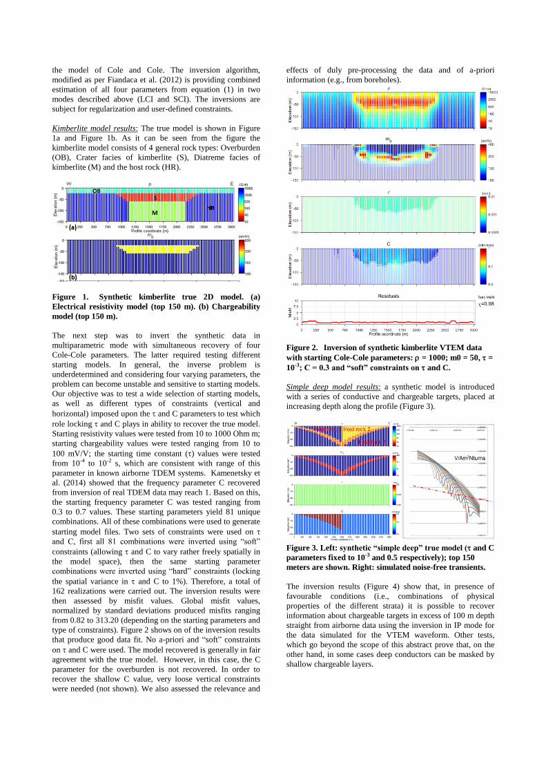
the model of Cole and Cole. The inversion algorithm,
modified as per Fiandaca et al. (2012) is providing combined
estimation of all four parameters from equation (1) in two
modes described above (LCI and SCI). The inversions are
subject for regularization and user-defined constraints.
Kimberlite model results: The true model is shown in Figure
1a and Figure 1b. As it can be seen from the figure the
kimberlite model consists of 4 general rock types: Overburden
(OB), Crater facies of kimberlite (S), Diatreme facies of
kimberlite (M) and the host rock (HR).
Figure 1. Synthetic kimberlite true 2D model. (a)
Electrical resistivity model (top 150 m). (b) Chargeability
model (top 150 m).
The next step was to invert the synthetic data in
multiparametric mode with simultaneous recovery of four
Cole-Cole parameters. The latter required testing different
starting models. In general, the inverse problem is
underdetermined and considering four varying parameters, the
problem can become unstable and sensitive to starting models.
Our objective was to test a wide selection of starting models,
as well as different types of constraints (vertical and
horizontal) imposed upon the and C parameters to test which
role locking and C plays in ability to recover the true model.
Starting resistivity values were tested from 10 to 1000 Ohm m;
starting chargeability values were tested ranging from 10 to
100 mV/V; the starting time constant () values were tested
from 10-4 to 10-2 s, which are consistent with range of this
parameter in known airborne TDEM systems. Kamenetsky et
al. (2014) showed that the frequency parameter C recovered
from inversion of real TDEM data may reach 1. Based on this,
the starting frequency parameter C was tested ranging from
0.3 to 0.7 values. These starting parameters yield 81 unique
combinations. All of these combinations were used to generate
starting model files. Two sets of constraints were used on
and C, first all 81 combinations were inverted using “soft”
constraints (allowing and C to vary rather freely spatially in
the model space), then the same starting parameter
combinations were inverted using “hard” constraints (locking
the spatial variance in and C to 1%). Therefore, a total of
162 realizations were carried out. The inversion results were
then assessed by misfit values. Global misfit values,
normalized by standard deviations produced misfits ranging
from 0.82 to 313.20 (depending on the starting parameters and
type of constraints). Figure 2 shows on of the inversion results
that produce good data fit. No a-priori and “soft” constraints
on and C were used. The model recovered is generally in fair
agreement with the true model. However, in this case, the C
parameter for the overburden is not recovered. In order to
recover the shallow C value, very loose vertical constraints
were needed (not shown). We also assessed the relevance and
effects of duly pre-processing the data and of a-priori
information (e.g., from boreholes).
Figure 2. Inversion of synthetic kimberlite VTEM data
with starting Cole-Cole parameters: = 1000; m0 = 50, =
10-3; C = 0.3 and “soft” constraints on and C.
Simple deep model results: a synthetic model is introduced
with a series of conductive and chargeable targets, placed at
increasing depth along the profile (Figure 3).
Figure 3. Left: synthetic “simple deep” true model ( and C
parameters fixed to 10-3 and 0.5 respectively); top 150
meters are shown. Right: simulated noise-free transients.
The inversion results (Figure 4) show that, in presence of
favourable conditions (i.e., combinations of physical
properties of the different strata) it is possible to recover
information about chargeable targets in excess of 100 m depth
straight from airborne data using the inversion in IP mode for
the data simulated for the VTEM waveform. Other tests,
which go beyond the scope of this abstract prove that, on the
other hand, in some cases deep conductors can be masked by
shallow chargeable layers.

Figure 4. Inversion of synthetic VTEM data for “simple
deep” model in IP mode with the following starting model
parameters: = 1000; m0 = 10, = 10-3; C = 0.5 and
“hard” constraints on and C.
Amakinskaya Kimberlite pipe results: From the geological
standpoint, the area surrounding Amakinskaya kimberlite pipe
belongs to a sedimentary basin with widespread outcrops of
clays and alevrolites of Jurassic age (J1or), which
unconformably overlay Cambrean limestone complex (Є3hl).
Triassic basalts (T1kt) are also widespread in the area,
especially to the north from the pipe. Amakinskaya
Kimberlite pipe shows a great deal of anisotropy in the
vertical direction, shifting from weathered, clayish upper
facies, affected by permafrost to consolidated hard kimberlite
below 30 m depth. This obviously has reflection in the
physical properties of the kimberlite. Resistivity and
chargeability changes with depth, showing lowering resistivity
and increasing chargeability values in the upper facies of the
kimberlite, while magnetic susceptibility increases with depth,
as kimberlite consolidates (Bondarenko and Zinchuk, 2004).
The airborne survey was flown in late 2014 using a VTEM
system and the data were seriously affected by the IP effect
(Figure 5b). It should be noted however, that IP effect over
the kimberlite, although evident in the transients, does not
result in negative voltage measurements and therefore may not
be instantly obvious in the data space at a first glance.
Figure 5. Location of Amakinskaya kimberlite pipe (north-
eastern Russia); (a): VTEM flight lines shown over
Landsat image. (b): IP effect measured over the kimberlite,
shown in VTEM individual transients.
In addition to strong IP effect, which made conventional
inversion challenging, there was a strong electrified industrial
infrastructure situated just 200 meters east of the Amakinskaya
pipe, which seriously affected both EM and magnetic data.
This cultural noise had to be removed from all data sets in
order to proceed further with inverting the data. In general,
the IP effect may be indicative of the clay alteration, which, in
turn, may be present in upper (weathered) facies of a
kimberlite. Interpretation of IP effect over kimberlites for
ground TDEM surveys has been previously described in the
literature (Kamenetsky et al., 2014) and becomes increasingly
attractive in case with airborne TDEM data sets, as it allows
extraction of chargeability, along with other parameters, such
as time constant () and frequency parameter (C).
As a result of SCI inversion approach with IP modelling, all
four Cole-Cole parameters were extracted. The target misfits
of the inversions were achieved, producing distributions of
Cole-Cole parameters, which were further interpolated to
populate 3D volumes. The distributions of electrical
resistivity and chargeability with depth are shown in Figure 6.
Overall, the results of the inversions allow to clearly
differentiate between the kimberlite and the host rock. The
results are shown in Figure 7 as a compilation of all inversion
results (including Mag), interpolated along VTEM flight line
9310 and shown as a depth section of electrical resistivity,
chargeability and magnetic susceptibility.
Figure 6. 3D distribution of electrical resistivity and
chargeability recovered by SCI inversion with IP
modelling over Amakinskaya kimberlite pipe, shown as
series of depth slices.
The physical properties recovered through inversion of the
VTEM data were compared to those derived from laboratory
measurements on kimberlite samples (Figure 8). There is good
agreement on the resistivity of the different facies, from the
weathered kimberlite top to the deeper kimberlite breccia and
carboniferous kimberlite. The clean limestones in the
laboratory data display higher resistivities than those
recovered by VTEM, due to the effect of saline water known
to be present in the limestones, forming a confined aquifer in
the area.
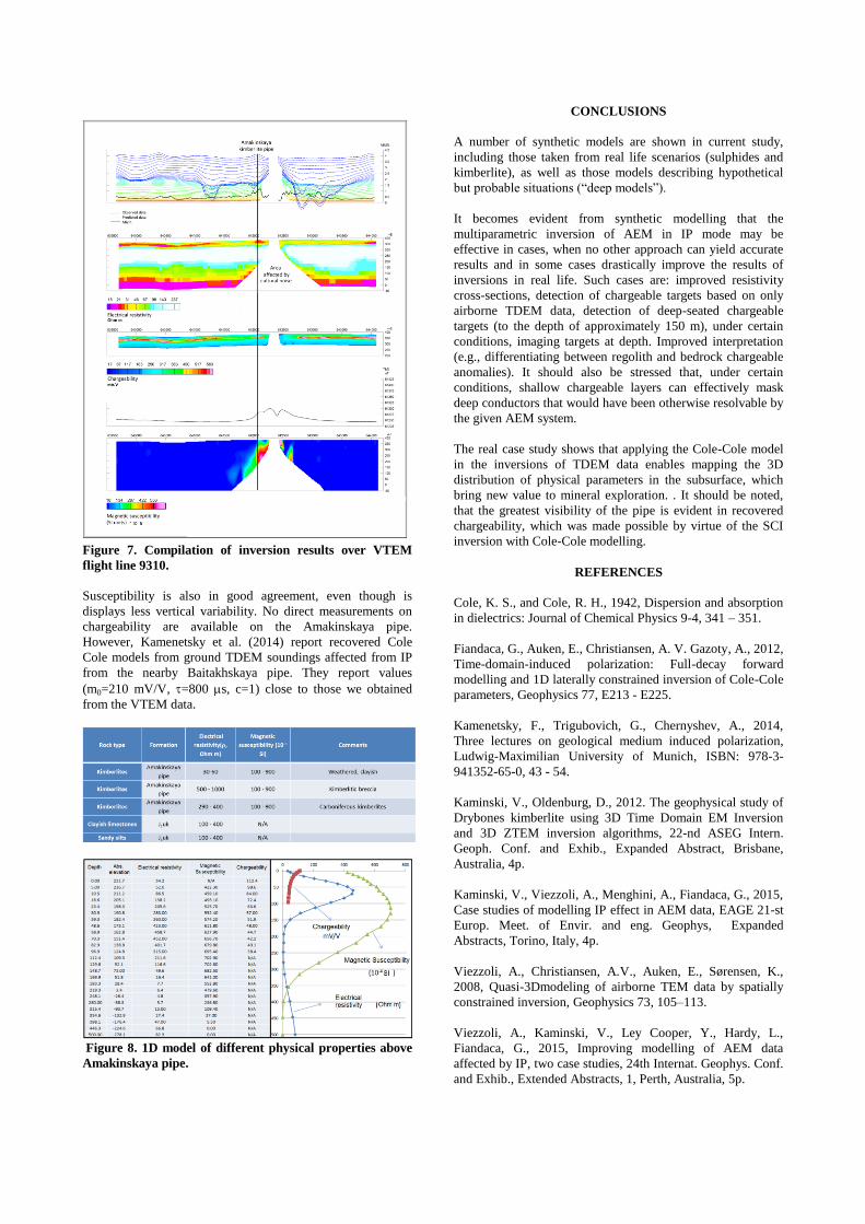
Figure 7. Compilation of inversion results over VTEM
flight line 9310.
Susceptibility is also in good agreement, even though is
displays less vertical variability. No direct measurements on
chargeability are available on the Amakinskaya pipe.
However, Kamenetsky et al. (2014) report recovered Cole
Cole models from ground TDEM soundings affected from IP
from the nearby Baitakhskaya pipe. They report values
(m0=210 mV/V, =800 s, c=1) close to those we obtained
from the VTEM data.
Figure 8. 1D model of different physical properties above
Amakinskaya pipe.
CONCLUSIONS
A number of synthetic models are shown in current study,
including those taken from real life scenarios (sulphides and
kimberlite), as well as those models describing hypothetical
but probable situations (“deep models”).
It becomes evident from synthetic modelling that the
multiparametric inversion of AEM in IP mode may be
effective in cases, when no other approach can yield accurate
results and in some cases drastically improve the results of
inversions in real life. Such cases are: improved resistivity
cross-sections, detection of chargeable targets based on only
airborne TDEM data, detection of deep-seated chargeable
targets (to the depth of approximately 150 m), under certain
conditions, imaging targets at depth. Improved interpretation
(e.g., differentiating between regolith and bedrock chargeable
anomalies). It should also be stressed that, under certain
conditions, shallow chargeable layers can effectively mask
deep conductors that would have been otherwise resolvable by
the given AEM system.
The real case study shows that applying the Cole-Cole model
in the inversions of TDEM data enables mapping the 3D
distribution of physical parameters in the subsurface, which
bring new value to mineral exploration. . It should be noted,
that the greatest visibility of the pipe is evident in recovered
chargeability, which was made possible by virtue of the SCI
inversion with Cole-Cole modelling.
REFERENCES
Cole, K. S., and Cole, R. H., 1942, Dispersion and absorption
in dielectrics: Journal of Chemical Physics 9-4, 341 – 351.
Fiandaca, G., Auken, E., Christiansen, A. V. Gazoty, A., 2012,
Time-domain-induced polarization: Full-decay forward
modelling and 1D laterally constrained inversion of Cole-Cole
parameters, Geophysics 77, E213 - E225.
Kamenetsky, F., Trigubovich, G., Chernyshev, A., 2014,
Three lectures on geological medium induced polarization,
Ludwig-Maximilian University of Munich, ISBN: 978-3-
941352-65-0, 43 - 54.
Kaminski, V., Oldenburg, D., 2012. The geophysical study of
Drybones kimberlite using 3D Time Domain EM Inversion
and 3D ZTEM inversion algorithms, 22-nd ASEG Intern.
Geoph. Conf. and Exhib., Expanded Abstract, Brisbane,
Australia, 4p.
Kaminski, V., Viezzoli, A., Menghini, A., Fiandaca, G., 2015,
Case studies of modelling IP effect in AEM data, EAGE 21-st
Europ. Meet. of Envir. and eng. Geophys, Expanded
Abstracts, Torino, Italy, 4p.
Viezzoli, A., Christiansen, A.V., Auken, E., Sørensen, K.,
2008, Quasi-3Dmodeling of airborne TEM data by spatially
constrained inversion, Geophysics 73, 105–113.
Viezzoli, A., Kaminski, V., Ley Cooper, Y., Hardy, L.,
Fiandaca, G., 2015, Improving modelling of AEM data
affected by IP, two case studies, 24th Internat. Geophys. Conf.
and Exhib., Extended Abstracts, 1, Perth, Australia, 5p.