Short Selling and Earnings Management:

A Controlled Experiment*

Vivian W. Fang a

University of Minnesota

Allen H. Huang b

Hong Kong University of Science and Technology

Jonathan Karpoff c

University of Washington

This draft: November 16, 2014

Abstract

During 2005-2007, the SEC ordered a pilot program in which one-third of the Russell 3000 were

arbitrarily chosen as pilot stocks and exempted from short-sale price tests. Pilot firms’ discretionary

accruals and likelihood of marginally beating earnings targets decrease during this period, and revert to

pre-experiment levels when the program ends. After the program starts, pilot firms are more likely to be

caught for fraud initiated before the program, and their stock returns better incorporate earnings

information. These results indicate that short selling, or its prospect, works to curb earnings management,

helps to detect fraud, and improves price efficiency.

JEL classifications: G14; G18; G19; M41; M48

Keywords: Regulation SHO; Pilot Program; Short Selling; Earnings Management; Fraud Discovery;

Price Efficiency

______________________________

*

We are grateful for helpful comments from two anonymous referees, an anonymous associate editor, Kenneth

Singleton (the editor), Vikas Agarwal, Mark Chen, John Core, Hemang Desai, Jarrad Harford, Adam Kolasinski,

Paul Ma, Scott Richardson, Ed Swanson, Jake Thornock, Wendy Wilson, and seminar participants at Cheung Kong

Graduate School of Business, Peking University, CEAR/GSU Finance Symposium on Corporate Control

Mechanisms and Risk, FARS Midyear Meeting, HKUST Accounting Symposium, CFEA Conference, and UC

Berkeley Multi-disciplinary Conference on Fraud and Misconduct. We are grateful to Russell Investments for

providing the list of 2004 Russell 3000 index, and to Jerry Martin for providing the KKLM data on financial

misrepresentation. Huang gratefully acknowledges financial support from a grant from the Research Grants Council

of the HKSAR, China (Project No., HKUST691213).

a Email: fangw@umn.edu, Carlson School of Management, University of Minnesota, Minneapolis, MN 55455,

USA. b Email: allen.huang@ust.hk, The Hong Kong University of Science and Technology, Clear Water Bay, Kowloon,

Hong Kong c Email: karpoff@uw.edu, Foster School of Business, University of Washington, Seattle, WA 98195, USA.

1

Short Selling and Earnings Management: A Controlled Experiment

I. Introduction

Previous research shows that short sellers can identify earnings manipulation and fraud before

they are publicly revealed.1 But this is for earnings manipulations that already have taken place. Might

short selling also constrain firms’ incentives to manipulate or misrepresent earnings in the first place?

That is, does the prospect of short selling help improve the quality of firms’ financial reporting?

In this paper we exploit a natural experiment that allows us to address this question. In July 2004,

the Securities and Exchange Commission (SEC) adopted a new regulation governing short selling

activities in the U.S. equity markets – Regulation SHO. Regulation SHO contained a Rule 202T pilot

program in which every third stock ranked by trading volume within each exchange was drawn from the

Russell 3000 index and designated as a pilot stock. From May 2, 2005 to August 6, 2007, pilot stocks

were exempted from short-sale price tests, including the tick test for exchange-listed stocks and the bid

test for Nasdaq National Market Stocks.2

The pilot program creates an ideal setting to examine the effect of short selling on corporate

financial reporting decisions, for three reasons. First, the exemption from short-sale price tests decreased

the cost of short selling in the pilot stocks relative to the non-pilot stocks (see the SEC’s Office of

Economic Analysis, 2007; Diether, Lee, and Werner, 2009). The pilot program thus eliminates the need

to estimate short selling costs directly, a notoriously difficult task (see Lamont, 2012). Rather, we use the

fact that the prospect of short selling increased in the pilot firms relative to the non-pilot firms, all else

being equal. Second, the pilot program represents a truly exogenous shock to the cost of selling short in

the affected firms. We can identify no evidence that the firms themselves lobbied for the pilot program,

or that any individual firm could know it would be in the pilot group until the program was announced.

1 See Dechow, Sloan, and Sweeney (1996), Christophe, Ferri, and Angel (2004), Efendi, Kinney, and Swanson

(2005), Desai, Krishnamurthy, and Venkataraman (2006), and Karpoff and Lou (2010). 2 The pilot program was originally scheduled to commence on January 3, 2005 and end on December 31, 2005

(Securities Exchange Act Release No. 50104, July 28, 2004). However, the SEC postponed the commencement date

to May 2, 2005 (Securities and Exchange Act Release No. 50747, November 29, 2004) and extended the end date to

August 6, 2007 (Securities and Exchange Act Release No. 53684, April 20, 2006).

2

Third, the pilot program had specific beginning and ending dates, facilitating a difference-in-differences

(hereafter, DiD) analysis of the impact of short selling costs on firms’ financial reporting. The known

ending date allows us to investigate whether the effects of the pilot program reversed when it ended – an

important check on the internal validity of the DiD tests (e.g., see Roberts and Whited, 2012).

We begin by verifying that pilot firms represent a random draw from the Russell 3000 population.

In the fiscal year before the pilot program, the pilot and non-pilot firms are similar in size, growth,

corporate spending, profitability, leverage, and dividend payout. Although the two groups of firms also

exhibit similar levels of discretionary accruals before the program, pilot firms significantly reduce their

discretionary accruals once the program starts.3 After the program ends, pilot firms’ discretionary

accruals revert to pre-program levels. The non-pilot firms, meanwhile, show no significant change in

their discretionary accruals around the pilot program. Our point estimates indicate that performance-

matched discretionary accruals, as a percentage of assets, are one percentage point lower for the pilot

firms than for the non-pilot firms during the three-year pilot program compared to the three-year pre-pilot

period. This corresponds to 7.4% of the standard deviation of discretionary accruals in our sample.

We also examine the pilot program’s effect on two alternative measures of earnings management.

First, we find that the likelihood of beating the analyst consensus forecast by up to one cent is 1.8

percentage points lower for the pilot firms than the non-pilot firms during the pilot program. This

represents 11.1% of the unconditional likelihood of meeting or just beating analysts’ forecast in our

sample. Similarly, the likelihood of meeting or just beating the firm’s quarterly EPS in the same quarter

of the prior year is 0.8 percentage points lower for the pilot firms, representing 14.2% of the

unconditional likelihood. Second, we find that the likelihood of being classified as a misstating firm,

based on the F-score of Dechow et al. (2011), is significantly lower for the pilot firms during the pilot

3 Following the literature (e.g., Kothari, Leone, and Wasley, 2005), we measure discretionary accruals as the

difference between actual accruals and a benchmark estimated within each industry-year. Details are provided in

Section III.C.

3

period. Combined with our results regarding discretionary accruals, these results indicate that pilot firms

decrease their earnings management during the pilot program.

We consider several alternative interpretations for the patterns we observe in discretionary

accruals. One possibility is that pilot firms’ discretionary accruals reflect changes in their growth,

investment, or equity issuance, as Grullon, Michenaud, and Weston (2014) document a significant

reduction in financially constrained pilot firms’ investment and equity issuance during the pilot program.

We consider several controls for firm growth and investment, both in the construction of our discretionary

accruals measures and as controls in the multivariate tests. None of these controls has a material effect on

our main findings. We also find that the pilot firms’ investment levels do not follow a pattern that would

explain the changes in their discretionary accruals during and after the pilot program. Regarding the

possible impact of equity issuance, we find that pilot firms’ discretionary accruals pattern is similar

among firms that do not seek to issue equity as for the overall sample. These results indicate that the

effect of the pilot program on discretionary accruals is unlikely to be explained by changes in pilot firms’

growth, investment, or equity issuance surrounding the program.

Another possible explanation is that managers of the pilot firms decreased their earnings

management because of a general increase in investors’ attention paid to these firms. Using three

measures of market attention, however, we do not find that pilot firms were subject to greater attention

during the pilot program. In multivariate DiD tests, the market attention measures are not significantly

related to discretionary accruals, nor do they affect our main finding in discretionary accruals.

The most plausible interpretation of our results is that the pilot program reduced the cost of short

selling sufficiently among the pilot firms to increase potential short sellers’ monitoring activities, and that

the increased monitoring induced a decrease in these firms’ earnings management.4 We conduct three

additional tests to further probe this interpretation. First, we find that, among the pilot firms during the

pilot program, short selling is positively related to discretionary accruals. Second, we find that short

4 Throughout this paper, we use “potential short sellers” or “short sellers” to refer both to investors who may take

new short positions and investors with existing short positions.

4

interest increases in months in which firms are later revealed to have engaged in financial

misrepresentation during our sample period. And third, we find that, among firms that had previously

initiated financial fraud, pilot firms are more likely to get caught than control firms after the pilot period

started. We also find that the unconditional likelihood that pilot firms are caught for financial fraud

converges monotonically toward that for non-pilot firms as we sequentially include frauds initiated after

the pilot program begins. This result is consistent with both an increase in the pilot firms’ conditional

likelihood of being caught for any financial frauds they commit, and our finding that pilot firms

endogenously adjust by decreasing their earnings manipulations after the pilot program begins.

Finally, we examine the implications of the pilot program for price efficiency through its effect

on firms’ reporting practices. We show that the pilot firms’ coefficients of current returns on future

earnings increase. Among firms announcing particularly negative earnings surprises, the well-

documented post-earnings announcement drift disappears for pilot firms during the pilot period, while it

remains significant for non-pilot firms. These results indicate that the reduction in pilot firms’ earnings

management during the pilot program corresponds to an increase in the efficiency of their stock prices as

their stock returns better incorporate earnings information.

These findings make four contributions to the literature. First, they show that an increase in the

prospect of short selling has real effects on firms’ financial reporting. This demonstrates one avenue

through which trading in secondary financial markets affects firms’ decisions.5 Second, our results

highlight one important avenue through which short selling improves price discovery and makes prices

more efficient. Previous research emphasizes how short selling facilitates the flow of private information

into prices (e.g., Miller, 1977; Harrison and Kreps, 1978; Chang, Cheng, and Yu, 2007; Boehmer and Wu

2013). Our findings indicate that the prospect of short selling also improves price efficiency by

decreasing managers’ tendency to manage earnings. Third, our findings identify a new determinant of

5 See Bond, Edmans, and Goldstein (2012) for a survey of research on the real effects of financial markets. For

example, Karpoff and Rice (1989) and Fang, Noe, and Tice (2009) examine the effect of stock liquidity on firm

performance; Fang, Tian, and Tice (2014) examine the effect of liquidity on innovation; and Grullon, Michenaud,

and Weston (2014) examine the effect of short selling constraints on investment and equity issuance.

5

earnings management – short-sale constraints – in addition to the factors identified in prior research (for a

review, see Dechow, Ge, and Schrand, 2010). And fourth, these results contribute to the policy debate on

the benefits and costs of short selling. Previous research demonstrates that short sellers frequently are

good at identifying the overpriced shares of firms that have manipulated earnings, and that short sellers’

trading conveys external benefits to other investors by improving market quality and by accelerating the

discovery of financial misconduct.6 Our results indicate that the prospect of short selling decreases

earnings management and increases price efficiency in general, even among firms that are not charged

with financial reporting violations. This indicates that short selling, or its prospect, conveys external

benefits to investors by improving financial reporting quality and stock price efficiency.

This paper is organized as follows. Section II describes short-sale price tests in the U.S. equity

markets, how they can affect firms’ tendency to manage earnings, and related research. Section III

describes the data. Section IV reports tests of the effect of Regulation SHO’s pilot program on firms’

earnings management. Section V examines whether short sellers actually increased their scrutiny of the

pilot stocks during the pilot program by comparing the probability of fraud detection between pilot and

non-pilot firms. Section VI reports on tests that examine whether the pilot program coincided with an

increase in the efficiency of pilot firms’ stock prices with respect to earnings, and Section VII concludes.

II. Short-sale price tests, its effect on earnings management, and related research

A. Short-sale price tests in U.S. equity markets

Short-sale price tests were initially introduced to the U.S. equity markets in the 1930s, ostensibly

to avoid bear raids by short sellers in declining markets. The NYSE adopted an uptick rule in 1935,

which was replaced in 1938 by a stricter SEC rule, Rule 10a-1, also known as the “tick test.” The rule

mandates that a short sale can only occur at a price above the most recently traded price (plus tick) or at

6 See the references in footnote 1, and also the SEC’s Office of Economic Analysis (2007), Alexander and Peterson

(2008), and Diether, Lee, and Werner (2009). To be sure, other studies have noted the potential dark side of short

selling, as manipulative short selling could reduce price efficiency (e.g., Gerard and Nanda, 1993; Henry and Koski,

2010).

6

the most recently traded price if that price exceeds the last different price (zero-plus tick).7 In 1994, the

NASD also adopted its own price test (the “bid test”) under Rule 3350. Rule 3350 requires a short sale to

occur at a price one penny above the bid price if the bid is a downtick from the previous bid.8

To facilitate research on the effects of short-sale price tests on financial markets, the SEC

initiated a pilot program under the Rule 202T of Regulation SHO in July 2004. Under the pilot program,

every third stock in the Russell 3000 index ranked by trading volume was selected as a pilot stock. From

May 2, 2005 to August 6, 2007, pilot stocks were exempted from short-sale price tests. Subsequent to the

pilot program, on July 6, 2007, the SEC eliminated short-sale price tests for all exchange-listed stocks.

The decision to eliminate all short-sale price tests prompted a huge backlash from managers and

politicians. In 2008, NYSE Euronext commissioned Opinion Research Corporation to conduct a study to

seek corporate issuers’ views on short selling. Fully 85% of the surveyed corporate managers favored

reinstituting the short-sale price tests “as soon as practical,” indicating that managers are aware of and

sensitive to the impact of eliminating price tests on the potential amount of short selling in their firms.

The former state banking superintendent of New York argued that the SEC’s repeal of the price tests

added to market volatility, especially in down markets.9 The Wall Street Journal argued that the SEC’s

Office of Economic Analysis (2007) was too biased to evaluate the short-sale price tests fairly.10

Wachtell, Lipton, Rosen & Katz, a well-known law firm, argued that the uptick rule should be reinstated

immediately, and three members of Congress introduced a bill (H.R. 6517) to require the SEC to reinstate

the uptick rule. Presidential candidate Sen. John McCain blamed the SEC for the recent financial turmoil

by “turning our markets into a casino,” in part because of the increased prospect of short sales, and called

7 Narrow exceptions apply, as specified in SEC’s Rule 10a-1, section (e).

8 Rule 3350 applies to Nasdaq National Market (Nasdaq NM or NNM) securities. Securities traded in the OTC

markets, including Nasdaq Small Cap, OTCBB, and OTC Pink Sheets, are exempted. When Nasdaq became a

national listed exchange in August 2006, NASD Rule 3350 was replaced by Nasdaq Rule 3350 for Nasdaq Global

Market securities (formerly Nasdaq NM securities) traded on Nasdaq, and NASD Rule 5100 for Nasdaq NM

securities traded over-the-counter. The Nasdaq switched from fractional pricing to decimal pricing over the interval

of March 12, 2001 – April 9, 2001. Prior to decimalization, Rule 3350 required a short sale to occur at a price 1/8th

dollar (if before June 2, 1997) or 1/16th

dollar (if after June 2, 1997) above the bid. 9 Gretchen Morgenson, “Why the roller coaster seems wilder,” The New York Times, August 26, 2007, Page 31.

10 “There’s a better way to prevent bear raids,” The Wall Street Journal, November 18, 2008, Page A19.

7

for the SEC’s chairman to be dismissed. In response to this pressure, the SEC partially reversed course

and restored a modified uptick rule on February 24, 2010. Under the new rule, price tests are triggered

when a security’s price declines by 10% or more from the previous day’s closing price. This policy

reversal drew sharp criticism itself, this time from hedge funds and short sellers.11

B. The impact of the pilot program on earnings management

The strong public reactions to changes in the uptick rule indicate that the rule is important to

investors, managers, and politicians. Consistent with practitioners’ perception, most prior research

indicates that short-sale price tests impose meaningful constraints on short selling, an assumption we

examine further in the next section.12

In this section, we draw from prior studies to construct our main

hypothesis about how changes in the cost of short selling due to the removal of short-sale price tests – and

the corresponding changes in the prospect of short selling – affect a manager’s tendency to engage in

earnings management.

Previous research indicates that executives have incentives to distort their firms’ reported

financial performance to bolster their compensation, gains through stock sales, job security, operational

flexibility, or control.13

This implies that managers can earn a personal benefit from managing earnings

to inflate the stock price. Prior research also demonstrates that short selling facilitates the flow of

unfavorable information into stock prices, increases price efficiency, and dampens the price inflation that

motivates managers to manipulate earnings in the first place (e.g., see Miller, 1977; Harrison and Kreps,

1978; Chang, Cheng, and Yu, 2007; Karpoff and Lou, 2010; Boehmer and Wu, 2013). These findings

indicate that managers’ benefits of manipulating earnings decrease with the prospect of short selling

11

See “Hedge Funds Slam Short-Sale Rule,” The New York Times, February 25, 2010. 12

See, for examples, McCormick and Reilly (1996), Angel (1997), Alexander and Peterson (1999, 2008), the SEC’s

Office of Economic Analysis (2007), and Diether, Lee, and Werner (2009). For a contradictory finding, however,

see Ferri, Christophe, and Angel (2004). 13

For evidence regarding compensation motives, see Bergstresser and Philippon (2006), Burns and Kedia (2006),

and Efendi, Srivastava, and Swanson (2007); regarding stock sale motives, see Beneish and Vargus (2002);

regarding job security and control-related motives, see DeFond and Park (1997), Ahmed, Lobo, and Zhou (2006),

DeFond and Jiambalvo (1994), and Sweeney (1994).

8

because short sellers’ activities partially offset the price inflation that motivates managers to manipulate

earnings in the first place.

Although earnings management conveys benefits to managers, managers cannot manipulate

earnings with impunity. Previous research shows that aggressive earnings management is associated with

an increased likelihood of forced CEO turnover (see Hazarika, Karpoff, and Nahata, 2012; Karpoff, Lee,

and Martin 2008), and that short sellers help to monitor managers’ reporting behavior and uncover

aggressive earnings management (see, e.g., Efendi, Kinney, and Swanson, 2005; Desai, Krishnamurthy,

and Venkataraman, 2006; and Karpoff and Lou, 2010). These results indicate that, for any given level of

earnings management, managers’ potential cost increases with a reduction in the cost of short selling and

an increase in the prospect of short sellers’ scrutiny.

Regulation SHO’s pilot program, which eliminated short-sale price tests for the pilot stocks,

represents an exogenously imposed reduction in the cost of short selling and an increase in the prospect of

short selling in these stocks. The effect is to decrease pilot firm managers’ expected benefits and to

increase their expected costs at any given level of earnings management. These effects on a manager’s

choice to manage earnings are illustrated in Figure 1. Let MB0 and MC0 represent the managers’ marginal

benefit and marginal cost of managing earnings before the initiation of the pilot program. In drawing

these curves with their normal slopes, we assume that the benefits from artificial stock price inflation

increase at a decreasing rate in the level of earnings management, while the costs from the prospect of

being discovered increase at an increasing rate. The pre-program optimum amount of earnings

management is EM0. Once the program starts, the marginal benefit and marginal cost of earnings

management shift to MB1 and MC1, and the manager adjusts endogenously by choosing a new, lower

level of earnings management, EM1. This adjustment among pilot firms implies our first hypothesis:

Hypothesis 1: Earnings management in the pilot firms will decrease relative to earnings

management in the non-pilot firms during the pilot program.

9

C. The impact of the pilot program on fraud discovery

In developing Hypothesis 1 we assume that the pilot program had a substantial enough effect on

short sellers’ activities to induce a measurable change in the pilot firms’ financial reporting decisions.

Previous research finds that, in general, short selling tracks firms’ discretionary accruals and that short

selling helps to uncover financial misrepresentation.14

In Section I of the Internet Appendix, we report

results that confirm these two findings in our sample; that is, pilot firms’ short selling is positively related

to these firms’ discretionary accruals during the pilot period, and short interest increases in months in

which firms are later revealed to have engaged in financial misrepresentation. These results are consistent

with the view that cost reduction introduced by the pilot program did provide sufficient incentives for

short sellers to increase their scrutiny of the pilot firms’ reporting behavior. In this section, we exploit the

unique features of the pilot program to construct a hypothesis and test for whether the pilot program also

increased pilot firms’ risk of detection for earnings manipulations that rise to the level of financial

misrepresentation or fraud.15

We begin by noting that there generally is a time lag between when a firm begins misrepresenting

its earnings and when the misrepresentation is detected. Karpoff and Lou (2010) report that this lag

varies across firms and has a median of 26 months in their sample. We therefore characterize a firm’s

conditional probability of being caught as:

Pr(Caught(t + n)|Fraud(t)) = δ ΣsmsSSP(t + s). (1)

14

Desai, Krishnamurthy, and Venkataraman (2006), Cao et al. (2006), Karpoff and Lou (2010), and Hirshleifer,

Teoh, and Yu (2011) all report that short selling tracks discretionary accruals. Desai, Krishnamurthy, and

Venkataraman (2006) find that short selling leads the announcement of earnings restatements, and Karpoff and Lou

(2010) find that short selling accelerates the rate at which misrepresentation is detected. 15

Karpoff et al. (2014) point out that many instances of financial misrepresentation do not include fraud charges.

We nonetheless use the term “fraud” to refer to any illegal misrepresentation that attracts SEC enforcement action.

10

In Eq. (1), Pr(Caught(t + n)|Fraud(t)) is the firm’s probability of being caught at time t + n conditional

on misrepresenting at time t, where n ≥ 0. SSP(t + s) is short selling potential at time t + s, and when t +

s falls within the pilot period we expect this potential to be higher for pilot firms. ms represents the

individual weight each period’s short selling potential contributes to the conditional probability of

detection, and depends on the wide range of non-short-selling factors that affect a firm’s probability of

being caught. We hypothesize that an increase in short selling potential will help to uncover aggressive

reporting, i.e., δ > 0. This leads to our second hypothesis,

Hypothesis 2: Conditional on misreporting, pilot firms are more likely than non-pilot firms to get

caught after the pilot program starts.

A challenge in testing Hypothesis 2 is that we do not directly observe the conditional probability

of detection, but rather, only the unconditional probability that a firm both commits fraud and is detected,

which can be expressed as:

Pr(Caught(t + n), Fraud(t)) = Pr(Fraud(t))×Pr(Caught(t + n)|Fraud(t)). (2)

To develop a test of Hypothesis 2, we exploit the time lag between the commission and detection of fraud.

Since the pilot firms were selected randomly, it is reasonable to assume that, before the pilot program was

announced in July 2004, the actual rate of fraud commission was equal between the pilot and non-pilot

firms, i.e., Pr(Fraud(t))pilot = Pr(Fraud(t))non-pilot for t < July 2004.16

This allows us to use the

unconditional probability of detection for frauds that were initiated before the pilot program was

16

We restrict t to the period before the announcement of the pilot program (in July 2004) to ensure that the rate of

fraud commission is equal across the two groups of firms. Whereas short sellers arguably begin to change their

behavior after the pilot program is implemented in May 2005, managers of pilot firms could change their reporting

behavior in response to the prospect of short selling as early as when they learn the identity of the pilot stocks in

July 2004.

11

announced in July 2004, but detected after the program started in May 2005, to infer the conditional

probability of getting caught. Specifically, Hypothesis 2 implies that

Pr(Caught(post-May 2005), Fraud(pre-July 2004))pilot >

Pr(Caught(Post-May 2005), Fraud(pre-July 2004))non-pilot.

Once the pilot program was announced, Hypothesis 1 implies that managers of the pilot firms will

start to adjust endogenously to the higher conditional probability of detection by decreasing their earnings

management. That is,

Pr(Fraud(t))pilot < Pr(Fraud(t))non-pilot for 𝑡 > July 2004.

The pilot program therefore has two offsetting effects on the unconditional probability of detection for

frauds committed after July 2004: pilot firms commit fewer frauds, but conditional on committing fraud,

they are more likely to be caught. This implies that the difference between pilot and non-pilot firms in the

unconditional likelihood of fraud detection will decrease as we consider frauds initiated after the July

2004 announcement of the pilot program. In Section V below we also test and find support for this

implication of Hypothesis 2.

D. Related research

Our investigation is related to the small but growing literature that exploits changes in short sale

regulations to examine the economic implications of short selling. Autore, Billingsley, and Kovacs

(2011), Frino, Lecce, and Lepone (2011), and Boehmer, Jones, and Zhang (2013) examine the impact of a

widespread ban on short selling in U.S. equity markets in 2008, and Beber and Pagano (2013) examine

the impacts of short selling bans around the world. These studies conclude that the bans decreased

various measures of market quality.

Using Regulation SHO’s Rule 202T pilot program, Alexander and Peterson (2008) find that order

execution and market quality improved for the pilot stocks during the pilot program. Diether, Lee, and

Werner (2009) and the SEC’s Office of Economic Analysis (2007) show that pilot stocks listed on both

12

the NYSE and Nasdaq experienced a significant increase in short-sale trades and short sales-to-share

volume ratio during the term of the pilot program. The former also shows that NYSE-listed pilot stocks

experienced a higher level of order-splitting, suggesting that short sellers applied more active trading

strategies. Other papers relate the pilot program to firm outcomes. Grullon, Michenaud, and Weston

(2014), for example, examine the effect of the pilot program on pilot firms’ stock prices, equity issuance,

and investment. Kecskés, Mansi, and Zhang (2013) study bond yields, De Angelis, Grullon, and

Michenaud (2014) study equity incentives, and He and Tian (2014) study corporate innovation.

In our main analyses, we use the controlled experiment created by the pilot program to examine

the effect of short selling costs on firms’ earnings management decisions. This experiment is well suited

for our research question, as it facilitates DiD comparisons of pilot vs. non-pilot firms’ earnings

management before, during, and after the pilot program. The DiD tests allow us to control for time trends

that may be common to both the pilot and non-pilot firms, and mitigate concerns about reverse causality

or correlated omitted variables (because the SEC assigned pilot stocks arbitrarily). This experimental

design is thus superior to a blanket ban of short selling that applies to the entire cross-section of firms

because the latter can be muddied by possible confounding events. For example, changes in accruals

following the blanket ban on short selling during the recent financial crisis could be associated with

economy-wide changes in investment opportunities rather than the changes in short selling regulations.

A contemporaneous paper by Massa, Zhang, and Zhang (MZZ, 2014) also investigates the

effects of short selling on firms’ earnings management. Whereas we use the pilot program’s removal of

short-sale price tests in U.S. markets to identify our tests, MZZ focus on 33 international markets and use

the amount of shares available for lending to measure short-selling potential. To address endogeneity,

MZZ use Exchange-traded Fund (ETF) ownership as an instrument for lending supply. Like us, MZZ

also infer that short selling plays a disciplinary role in deterring firms’ opportunistic reporting behavior.

13

III. Data

A. Sample

On July 28, 2004, the SEC issued its first pilot order (Securities Exchange Act Release No.

50104) and published a list of 986 stocks that would trade without being subject to any price tests during

the term of the pilot program (available at http://www.sec.gov/rules/other/34-50104.htm). To create this

list, the SEC started with 2004 Russell 3000 index members and excluded stocks that were not previously

subject to price tests (i.e., not listed on NYSE, AMEX, or Nasdaq NM) and stocks that went public or had

spin-offs after April 30, 2004. The remaining stocks were then sorted by their average daily dollar

volume computed from June 2003 through May 2004 within each of the three listing markets. Every

third stock (beginning with the second one) within each listing market was designated as a pilot stock.

To construct our sample, we start with the 2004 Russell 3000 index and also exclude stocks that

were not listed on the NYSE, AMEX, or Nasdaq NM, and stocks that went public or had spin-offs after

April 30, 2004. Based on the SEC’s pilot order, we identify an initial sample of 986 pilot stocks and

1,966 non-pilot stocks. An examination of the exchange distribution of these stocks shows that both the

pilot and non-pilot groups are representative of the Russell 3000 index, confirming the statistics reported

by the SEC. Specifically, of the 986 pilot stocks, 49.9% (492) are listed on the NYSE, 47.9% (472) on

the Nasdaq NM, and 2.2% (22) on the AMEX. The exchange distribution of non-pilot stocks is very

similar, with 50% (982) listed on the NYSE, 48% (944) on the Nasdaq NM, and 2% (40) on the AMEX.

In our tests, we delete firms in the financial services (SIC 6000-6999) and utilities industries (SIC

4900-4949) because disclosure requirements and accounting rules are significantly different for these

regulated industries. A further complication with financial stocks is the 2008 short-sale ban imposed on

this sector. We require data from the Compustat Industrial Annual Files to construct earnings

management proxies and control variables. In most tests, we require all firms to have data to calculate

firm characteristics across the entire sample period, 2001-2003 and 2005-2010. The resulting balanced

panel sample consists of 388 pilot firms and 709 non-pilot firms. If we relax this requirement, our

unbalanced panel sample contains 741-782 pilot firms and 1,504-1,610 non-pilot firms in the year

14

immediately before the announcement of the pilot program (i.e., 2003), depending on the data availability

to calculate a given firm characteristic. We emphasize the results from the balanced panel sample, but

also report results for the unbalanced sample. Throughout, the results are similar using either sample.

B. Key test variables

We create an indicator variable PILOT to denote firms with pilot stocks (pilot firms).

Specifically, PILOT equals one if a firm’s stock is designated as a pilot stock under Regulation SHO’s

pilot program and zero otherwise. Pilot firms constitute the treatment sample and non-pilot firms serve as

the control sample. We also construct three variables to indicate time periods: PRE equals one if a firm-

year’s fiscal end falls between January 1, 2001 and December 31, 2003 and zero otherwise; DURING

equals one if a firm-year’s fiscal end falls between January 1, 2005 and December 31, 2007 and zero

otherwise; and POST equals one if a firm-year’s fiscal end falls between January 1, 2008 and December

31, 2010 and zero otherwise. In our primary DiD tests, we omit year 2004 because the identity of the

pilot and non-pilot stocks was made public in July 2004, so it is not clear whether year 2004 should be

classified as pre- or during-pilot period. In Table IA4 of the Internet Appendix, we report tests that

indicate our main findings are not substantially affected if we include the entire year of 2004 in the PRE

or Q1-Q3 of 2004 in the PRE and Q4 in the DURING period.

C. Measures of earnings management

Our primary proxy for earnings management is the performance-matched discretionary accrual

measure of Kothari, Leone, and Wasley (2005). To construct this measure, we first estimate the following

cross-sectional model within each fiscal year and Fama-French 48 industry,

𝑇𝐴𝑖,𝑡

𝐴𝑆𝑆𝐸𝑇𝑖,𝑡−1= 𝛽0+𝛽1

1

𝐴𝑆𝑆𝐸𝑇𝑖,𝑡−1+ 𝛽2

∆𝑅𝐸𝑉𝑖,𝑡

𝐴𝑆𝑆𝐸𝑇𝑖,𝑡−1+ 𝛽3

𝑃𝑃𝐸𝑖,𝑡

𝐴𝑆𝑆𝐸𝑇𝑖,𝑡−1+ 𝜀𝑖,𝑡. (3)

15

where i indexes firms and t indexes fiscal years. Total accruals TAt are defined as earnings before

extraordinary items and discontinued operations minus operating cash flows for fiscal year t, ASSETt-1 is

total assets at the end of year t − 1, ΔREVt is the change in sales revenue from year t − 1 to t, and PPEt is

the gross value of property, plant and equipment at the end of year t. We require at least 10 observations

to perform each cross-sectional estimation.

Next, we use the following model and the estimated coefficients from Eq. (3) to compute the

fitted normal accruals NAi,t,

𝑁𝐴𝑖,𝑡 = 𝛽0̂ + 𝛽1̂1

𝐴𝑆𝑆𝐸𝑇𝑖,𝑡−1+ 𝛽2̂

(∆𝑅𝐸𝑉𝑖,𝑡−∆𝐴𝑅𝑖,𝑡)

𝐴𝑆𝑆𝐸𝑇𝑖,𝑡−1+ 𝛽3̂

𝑃𝑃𝐸𝑖,𝑡

𝐴𝑆𝑆𝐸𝑇𝑖,𝑡−1. (4)

Following Dechow, Sloan, and Sweeney (1995), the change in accounts receivable is subtracted from the

change in sales revenue as credit sales might also provide potential opportunity for accounting distortion.

After obtaining the fitted normal accruals NAi,t from Eq. (4), we calculate the firm-year specific

discretionary accruals as DAi,t = (TAi,t / ASSETi,t-1) − NAi,t.

Finally, we adjust the estimated discretionary accruals for performance. We match each sample

firm with another firm from the same fiscal year-industry that has the closest return-on-assets ratio as the

given sample firm. The performance-matched discretionary accruals, denoted as Discretionary accruals,

are then calculated as the firm-specific discretionary accruals minus the discretionary accruals of the

matched firm. Discretionary accruals is signed and constructed to be positively related to income-

increasing earnings management.17

17

We create three additional performance-matched discretionary accrual measures by removing the intercept term

from Eq. (3) and Eq. (4) and/or replacing ∆𝑅𝐸𝑉𝑖,𝑡

𝐴𝑆𝑆𝐸𝑇𝑖,𝑡−1 with

(∆𝑅𝐸𝑉𝑖,𝑡−∆𝐴𝑅𝑖,𝑡)

𝐴𝑆𝑆𝐸𝑇𝑖,𝑡−1 in Eq. (3). The results using these alternative

measures are reported in Table IA5 of the Internet Appendix and are consistent with those reported in the paper.

16

D. Firm characteristics

Similar to Grullon, Michenaud, and Weston (2014), we compare the pilot and non-pilot firms’

characteristics in the fiscal year immediately before the announcement of the pilot program, 2003. Table

1, Panel A reports on the balanced panel sample, in which we require a firm to have financial data

available to calculate firm characteristics and accrual measures in all years of the sample period. The

mean book value of assets in both groups is $3.7 billion. The two groups also exhibit similar mean and

median values of the market-to-book ratio, one-year growth in assets, capital expenditures-to-assets ratio,

R&D expenditures-to-assets ratio, annual return-on-assets ratio, cash flow-to-assets ratio, leverage, and

the levels of cash and dividends (both as a percentage of total assets). In none of these comparisons is the

difference statistically significant, which supports our contention that Regulation SHO’s pilot program is

a well-controlled experiment that is suitable for examining the effects of short-sale constraints.

Panel B of Table 1 reports similar comparisons for the larger unbalanced panel sample. Firms in

this sample are slightly smaller than those included in the balanced panel sample, with assets averaging

$2.9 billion versus $3.7 billion. As in Panel A, the pilot and non-pilot firms in the unbalanced panel

sample are similar to each other in the financial characteristics we examine. The sole exception is that the

median capital expenditure by pilot firms is slightly higher than that for the non-pilot firms.

IV. The effect of Regulation SHO’s pilot program on earnings management

A. The effect of the pilot program on earnings management: discretionary accruals

Table 2 reports the results of the univariate DiD tests examining Hypothesis 1 using our primary

measure of earnings management based on discretionary accruals. Panel A reports on the balanced panel

sample defined in Section III.A. The mean value of Discretionary accruals during the three-year period

before the pilot program (2001–2003), is -0.004 for both the pilot and non-pilot firms. The t-statistic for

the difference in means (i.e., the cross-sectional estimator -0.001) is -0.03, and the Wilcoxon z-statistic for

the difference in medians is 0.77, both insignificant. During the three-year period of the pilot program

(2005-2007), the mean value of Discretionary accruals decreases to -0.014 for the pilot firms while it

17

remains at -0.004 for the non-pilot firms. The mean difference becomes -0.011 (t-statistic = -2.09) and

the median difference is -0.008 (Wilcoxon z-statistic = -2.23), both significant at the 5% level. For the

three-year period after the pilot program (2008-2010), Discretionary accruals increases for the pilot firms

to a mean of zero, while it changes slightly for the non-pilot firms to -0.003. The mean difference in the

post-pilot period is 0.004 (t-statistic = 0.69), and the median difference is 0.001 (Wilcoxon z-statistic =

0.66), both insignificant. The bottom-left cell of Table 2 Panel A reports the time-series estimators,

which track the change in Discretionary accruals within each group of firms across the three periods.

The second column shows that the average Discretionary accruals drops by -0.011 (significant at the 5%

level) for the pilot firms from pre- to during- the pilot program, but bounces back by 0.013 (significant at

the 1% level) after the program ends. Consistent with this reverting pattern, the time-series estimator

comparing pilot firms’ average Discretionary accruals from pre- to post- pilot program is 0.003 and

insignificant. In contrast, the estimators in the fourth column are never significant, suggesting that non-

pilot firms’ Discretionary accruals does not change much over time.

The bottom-right cell of Table 2 Panel A reports on the DiD estimators. The mean DiD estimator

for Discretionary accruals from before to during the pilot program is -0.011 with a t-statistic of -1.67.

This difference is statistically significant at only the 10% level. However, the results from other tests

reported below, including multivariate DiD tests and the results from the unbalanced panel, are significant

at lower levels. The DiD estimator that tracks Discretionary accruals from during to after the pilot

program is 0.013 with a t-statistic of 2.06. In addition, the DiD estimator that compares Discretionary

accruals pre-program to post-program is statistically insignificant with a t-statistic of 0.32. The last two

DiD estimators demonstrate that the effect of the pilot program on discretionary accruals reverses when

the program ends – an important check on the internal validity of the DiD test.

We plot these univariate results in Figure 2 for a better illustration of the pattern in discretionary

accruals. As the figure shows, non-pilot firms’ discretionary accruals do not change much over the entire

sample period. The pilot firms’ discretionary accruals, similar to those of the non-pilot firms before the

18

pilot program, decrease significantly during the program, and then revert to levels that are similar to those

of the non-pilot firms after the program.

Panel B of Table 2 reports on the changes in Discretionary accruals using data from the

unbalanced panel sample in which we do not require firms to have financial data available for all years of

the sample period. The results are similar to those from the balanced panel sample even though we are

only able to calculate the cross-sectional estimators given the unbalanced sample.

Next, we extend the DiD test using multivariate regressions. To do so, we retain firm-year

observations for both pilot and non-pilot firms for the nine-year window (2001-2003 and 2005-2010)

surrounding Regulation SHO’s pilot program and estimate the following model:

Discretionary accrualsi,t = β0 + β1PILOTi×DURINGt + β2PILOTi×POSTt

+ β3PILOTi + β4DURINGt + β5POSTt + ɛi,t. (5)

The variables are as defined in Sections III.B and III.C. The benchmark period consists of the

three years before the pilot program (2001-2003). As previously discussed, year 2004 is omitted from

these tests because the identity of the pilot stocks was announced midway through 2004. The regression

results estimating Eq. (5) are reported in Column (1) of Table 3. The coefficients of interest are the two

DiD estimators, β1 and β2. The coefficient on PILOT×DURING, β1, is negative and significant at the 5%

level. The magnitude of β1 is consistent with the univariate DiD results reported in Table 2 and indicates

that Discretionary accruals (i.e., discretionary accruals as a percentage of total assets) is one percentage

point lower for the treatment group than for the control group during the three-year period of the pilot

program compared to the three-year period pre-pilot. This corresponds to 7.4% of the standard deviation

of Discretionary accruals in the pooled sample, 0.135. The coefficient on PILOT×POST, β2, is

insignificant, which once again demonstrates the reverting pattern as the difference between the pilot and

non-pilot firms’ discretionary accruals after the pilot program is not statistically different from that before

the program. The coefficient on PILOT, β3, is also insignificant, consistent with pilot and non-pilot firms

exhibiting similar levels of discretionary accruals before the pilot program. Consistent with prior

19

research, the regression’s R2 is low, indicating that most of the cross-sectional differences in discretionary

accruals are due to unmodeled factors.

In Column (2), we augment Eq. (5) by including four controls that have been shown to affect a

firm’s level of discretionary accruals (e.g., Kothari, Leone, and Wasley, 2005; Zang, 2012): the natural

logarithm of total assets (SIZE), market-to-book ratio (MB), return-on-assets (ROA), and leverage (LEV).

In Column (3), we further include eight year fixed effects from 2002-2003 and from 2005-2010, but omit

DURING and POST as well as the fixed effect for 2001 (the base year) to avoid multicollinearity. The

results are similar when we include these additional controls.

B. The effect of the pilot program on earnings management: alternative measures

In this section we examine whether our results based on discretionary accruals are robust using

two alternative measures of earnings management. First, we examine whether the pilot program

differentially affected firms’ likelihood of meeting or marginally beating analyst consensus forecast.

Graham, Harvey, and Rajgopal (2005) report that a large majority of CFOs consider it important to beat

the analyst consensus forecast and that they are willing to engage in earnings manipulations to do so. For

this reason, many papers (e.g., Bhojraj et al., 2009) infer earnings management from the tendency of firms

to meet or beat analyst consensus by up to one cent.

We follow prior research and run the following probit model on a panel of quarterly earnings

announcements that take place during the same nine-year window (2001-2003 and 2005-2010):

BEAT_ALYi,q= β0 + β1PILOTi×DURINGq + β2PILOTi×POSTq + β3PILOTi +

β4DURINGq + β5POSTq + ɛi,q. (6)

Subscript q indicates a fiscal quarter. The dependent variable BEAT_ALY is coded one for quarters in

which the firm’s reported EPS meets or beats the most recent analyst consensus forecast before the

earnings announcement by up to one cent. Both reported EPS and analyst forecasts are retrieved from

I/B/E/S. To calculate analyst consensus, we take each analyst’s latest forecast issued within 90 days of

20

the fiscal quarter end and before the earnings announcement, and require a firm-quarter to have at least

three analysts. PILOT is defined as before while the two time indicators are now based on the earnings

announcement date. That is, DURINGq (POSTq) equals one if quarter q’s earnings announcement takes

place during (post) the pilot period, and zero otherwise.

The regression results estimating Eq. (6) are reported in Column (1) of Table 4. Consistent with

our earlier results using discretionary accruals, the coefficient on our main variable of interest – the DiD

estimator (PILOT×DURING) – is negative and significant at the 5% level. The marginal effect of β1,

calculated using the methodology suggested in Ai and Norton (2003), indicates that the likelihood of

marginally beating analyst consensus is 1.8 percentage points lower for the treatment group than for the

control group during the three-year period of the pilot program compared to the three-year period pre-

pilot. This corresponds to 11.1% of the unconditional likelihood of BEAT_ALY in the sample, 16.2%.18

The coefficient on the second DiD estimator (PILOT×POST), β2, continues to be insignificant, indicating

that the difference between the pilot and non-pilot firms’ likelihood of marginally beating analyst

consensus in the post-pilot period is not statistically different from that pre-pilot. The coefficient on

PILOT, β3, also remains insignificant, consistent with pilot firms and non-pilot firms having similar

likelihood of marginally beating analyst consensus pre-pilot.

In Column (2), we include a list of controls previously shown to affect the likelihood of beating

analyst consensus. We largely follow Edmans, Fang, and Lewellen (2014) to construct these controls,

including the log of market capitalization (MV), market-to-book ratio (MB), return-on-assets ratio (ROA),

the log of analyst coverage (ALY_N), the log of average forecasting horizon (ALY_HORIZON), and

analyst forecast dispersion (ALY_DISP). We also include two proxies for real earnings management: the

18

Ai and Norton (2003) argue that the magnitude of the interaction effect in nonlinear regressions may not equal its

marginal effect and propose a way to correct for the interaction term’s magnitude and standard error. Le (1998) and

Kolasinski and Siegel (2010), however, argue that the coefficient on the interaction term is relevant even in a

nonlinear regression, especially when used to measure proportional rather than absolute marginal effects. In our

setting, the interaction effect calculated using the conventional linear method is only slightly higher (2% versus

1.8%). Nevertheless, we quote the economic significance based on Ai and Norton (2003)’s interaction measure to

stay on the conservative side.

21

change in R&D expenditures from quarter q − 4 to quarter q, ΔR&Dq, and the change in capital

expenditures, ΔCAPEXq, both scaled by total assets at the beginning of quarter q. Among these controls,

the market-to-book ratio is positively related to the likelihood of marginally beating analyst consensus

while forecast horizon, forecast dispersion, and an increase in R&D spending are negatively related to this

likelihood. The inclusion of these controls, however, does not significantly alter the magnitude or the

significance of the coefficients on the pilot-related variables.

Graham, Harvey, and Rajgopal (2005) report that an alternative benchmark firms might try to

beat is the firm’s EPS of the same quarter last year. We therefore repeat our tests using BEAT_EPS, an

indicator that equals one if the firm’s quarterly EPS meets or beats the prior year same quarter’s EPS by

up to one cent. The results are tabulated in Columns (3)-(4) of Table 4. The results are qualitatively

similar to those using BEAT_ALY, although the coefficient on PILOT×DURING is significant at only the

10% level. The weaker statistical significance is consistent with Brown and Caylor (2005)’s finding that

analyst consensus, and not the prior year’s earnings, has become the most important earnings target for

U.S. firms in recent years. Nonetheless, the economic significance remains sizable, as the likelihood of

marginally beating the prior year same quarter’s EPS is 0.8 percentage points lower for the treatment

group than for the control group during the three-year period of the pilot program compared to the three-

year pre-pilot period. This represents a 14.2% difference based on the unconditional likelihood of

BEAT_EPS in the sample, which is 5.3%.

Next, we examine whether the pilot program differentially affected firms’ likelihood of being

classified as a misstating firm based on the F-score. The F-score is the predicted probability of misstating

using fitted values of a model that Dechow et al. (2011) develop to characterize firms that are subject to

SEC enforcement actions for financial misconduct that include one or more Accounting and Auditing

Enforcement Release (AAER). The model includes balance sheet items (which are intended to capture

accrual quality and financial performance), and/or nonfinancial measures, off-balance sheet activities, and

market-based measures. The advantage of this measure is that it is correlated with an ex post indication

of earnings management, namely the incidence of SEC enforcement action for earnings manipulations.

22

We calculate three versions of the F-score, F1-F3, using the three different sets of coefficient

estimates provided in Dechow et al. (2011). The first set of coefficients is obtained from their Model (1),

which includes accrual quality and financial performance measures. The second set comes from their

Model (2), which includes all variables in Model (1) plus nonfinancial measures and off-balance sheet

activities. The third set comes from their Model (3), which further includes market-based measures. We

then define a binary variable, HF1, which stands for “High F-score” and is set equal to one if the firm’s

F1 is equal to or above the 99th percentile of the sample. HF2 and HF3 are defined similarly, based on

Dechow et al. (2011)’s second and third models.

The results, replacing Discretionary accruals with HF1-HF3 in Eq. (5), are reported in Table 5.

As shown, the coefficient on our main DiD estimator of interest, PILOT×DURING, is once again

negative and significant at the 5% level in all columns. The marginal effect in Column (1) indicates that

the likelihood of being classified as a misstating firm is 0.4 percentage points lower for the treatment

group than for the control group during the three-year period of the pilot program compared to the three-

year pre-pilot period. As before, the coefficients on PILOT are insignificant, indicating that the pilot and

non-pilot firms had similar probabilities of being classified as misstating firms before the pilot program

began. The results using the higher F-score variables do, however, differ in one respect from those using

discretionary accruals or the meet or beat measures of earnings management – the coefficients on

PILOT×POST are negative and significant at the 10% level or lower. This result suggests that there is a

prolonged effect of the pilot program on pilot firms’ earnings quality when it is measured by the high F-

score variables.

C. The effect of the pilot program on earnings management: alternative explanations

So far, our results indicate that the increase in the prospect of short selling due to the removal of

short-sale price tests is associated with a significant decrease in pilot firms’ earnings management.

Hypothesis 1 implies that this result reflects how the prospect of short selling works to curb firms’

opportunistic reporting behavior. In this section, we evaluate several alternatives to this explanation.

23

C.1. Growth/investment and equity issuance

Grullon, Michenaud, and Weston (2014) document that financially constrained pilot firms

significantly reduced their investment and equity issuance during the pilot program. So it is possible that

the pilot firms’ tendency to decrease their earnings management during the pilot program reflects changes

in the difference between the pilot and non-pilot firms’ investment and/or equity issuance around the pilot

program. This concern is particularly pertinent when discretionary accruals are used to measure earnings

management, because prior research shows that a firm’s accruals correlate with its growth (e.g., Fairfield,

Whisenant, and Yohn, 2003; Zhang, 2007; Wu, Zhang, and Zhang, 2010) and its incentives to issue

equity (e.g., Friedlan, 1994; Teoh, Welch, and Wong, 1998a, 1998b).

To investigate this concern, we adopt several controls for firms’ investment. We begin by re-

estimating Eq. (5) controlling for R&D expenditures (R&D) and capital expenditures (CAPEX), both

scaled by lagged total assets. The results are reported in Table 6. In Column (1), we include R&D and

CAPEX separately. In Column (2), we include the sum of the two, INVESTMENT. The coefficients on

the two DiD estimators, PILOT×DURING and PILOT×POST, are barely affected by the inclusion of

these controls. In Columns (3)-(4), we further include squared terms of the investment variables to

account for the possibility that the effect of investment on accruals may be non-linear. The main results

remain similar. In Column (5), we modify the Jones model by adding the market-to-book ratio to both

Eq. (3) and (4) when calculating the performance-matched discretionary accruals. That is, total accruals

are modeled as a function of the market-to-book ratio in addition to the changes in revenues (or revenues

adjusted for accounts receivable in Eq. (4)) and PPE (both scaled by total assets). The results are again

similar to those reported in Table 3.

As an additional probe for any investment effect on accruals, we examine changes in the

investment variables surrounding the pilot program for the two groups of firms. If discretionary accruals

reflect only growth, investment should follow a pattern around the pilot program that is similar to the

pattern in Discretionary accruals. In Table IA6 of the Internet Appendix, we re-estimate Eq. (5)

24

replacing Discretionary accruals with CAPEX in Column (1), and INVESTMENT in Column (2). Our

results in Column (1) are consistent with Grullon, Michenaud, and Weston (2014)’s finding that capital

expenditures decreased for the pilot firms relative to the non-pilot firms during the pilot program.

However, pilot and non-pilot firms’ capital expenditures do not appear to converge when the pilot

program ends, as the coefficient estimate on PILOT×POST is significantly negative and of a larger

magnitude than that on PILOT×DURING. We also find no evidence that pilot firms’ overall

INVESTMENT decreased during the pilot program, which is consistent with Grullon, Michenaud, and

Weston’s (2014) finding that investment decreased during the pilot program only among pilot firms that

are identified as financially constrained.

We also examine whether our findings regarding pilot firms’ discretionary accruals are

concentrated among firms that sought to issue equity during our sample period. To do so, we partition the

sample according to whether firms were likely to issue equity during the pilot period. As Kadan et al.

(2009) point out, recent equity issuance is positively correlated with the ex ante likelihood that a firm will

issue equity again. We thus classify firms that issued equity at least once in the two prior fiscal years, as

recorded in the Thomson Reuters Securities Data Company (SDC) Platinum database, as Equity Issuers,

and firms that did not as Non-Equity-Issuers. As an alternative test, we also partition the sample based on

whether, ex post, the firm issued equity in the given year. This alternative approach has an advantage of

identifying Equity Issuers based on firms’ actual equity issuance. A drawback, however, is that some

potential issuers could be mistakenly classified as Non-Equity-Issuers if they refrained from issuing

equity because of the pilot program.

The results are reported in Table 7. The left panel reports results when the sample is partitioned

on the ex ante measure of firms’ desire to issue equity, and the right panel reports the results using the ex

post measure. Using either partition, the coefficient on PILOT×DURING is statistically significant only

among the subsample of Non-Equity-Issuers. The coefficient on PILOT×DURING for the subsample of

Equity Issuers ranges from -0.027 to 0.006 but is not statistically significant in either panel. These results

indicate that the effect of the pilot program on discretionary accruals is widespread and is not limited to

25

firms that are likely to issue equity. Overall, the results in this section do not support the contention that

the pattern in discretionary accruals that we document is driven by changes in firms’ investment levels

and/or equity issuance.19

C.2. Market attention

Another possible explanation is that the pilot program brought widespread attention to the pilot

firms and these firms refrained from manipulating earnings in response to the increased attention from the

overall market rather than attention from short sellers in particular.

To examine this market attention hypothesis, we construct three measures of investors’ awareness

of and attention to individual companies. Our first measure follows Da, Engelberg, and Gao (2011), and

is based on the frequency with which a stock is searched on Google. This Search Volume Index (SVI)

arguably reflects retail investors’ awareness of and interest in a particular firm. Our second measure of

market attention is the number of earnings forecasts issued by sell-side financial analysts. Sell-side

financial analysts work for brokerage firms and their research is typically funded by trading commissions

paid by institutions. We conjecture that, if a pilot firm experiences an increase in attention from

institutional investors, the institutions’ demand for information will prompt analysts to exert more effort

in collecting information, thereby generating more frequent earnings forecasts (e.g., see Jacob, Lys, and

Neale, 1999). As a third measure of market attention, we use the total trading volume in the stock.

Trading volume can also increase as a result of a decrease in the cost of short selling, but for this measure

we will focus on the trading volume in the period between the identification of the pilot firms and the

implementation of the program. Presumably, an increase in the trading volume before the program was

19

The discretionary accrual measure is industry-adjusted. So it is possible that our finding that pilot firms’

discretionary accruals reverted to pre-program levels after the pilot program could reflect changes in non-pilot firms’

accruals rather than changes in pilot firms’ accruals. We examine this concern in Section II of the Internet

Appendix, and find that the convergence in pilot and non-pilot firms’ discretionary accruals after the pilot program

does partly reflect a decrease in total accruals among the non-pilot firms.

26

implemented is more likely to reflect an increase in investors’ awareness of the firm, whereas an increase

in trading volume after the program was implemented could reflect the lower shorting costs.

If the announcement of the pilot program led to an increase in market attention, the effect should

occur following the announcement date of the SEC’s first pilot order (i.e., July 28, 2004) when the pilot

firms were first identified. We begin our test by restricting the focus to year 2004 and calculating the DiD

estimator for each of the three attention measures from the pre-announcement period (January 1, 2004 to

July 27, 2004) to the post-announcement period (July 28, 2004 to December 31, 2004). As shown in

Panel A of Table IA7 of the Internet Appendix, none of the market attention DiD estimators are

statistically significant, indicating that the announcement of the pilot program did not substantially raise

market attention for the pilot firms compared to the non-pilot firms.

We then repeat the univariate DiD tests over our main sample period (2001-2003, 2005-2010).

Table IA7, Panel B reports the results. As shown, most of the DiD estimators for changes in market

attention remain statistically insignificant. There are only two statistically significant results, regarding

the changes in the SVI and the number of analyst earnings forecasts from during the pilot period to after

the pilot period. These results indicate that the increased market attention, if any, was greater for the non-

pilot firms.

Finally, we re-estimate Eq. (5) including two of our attention measures, the number of analyst

forecasts and total trading volume, as additional controls. We cannot include SVI as an additional control

because SVI only dates back to year 2004 while our main sample period starts from 2001. The results,

reported in Table IA8, remain similar to those in Table 3.

Market attention is an elusive concept that is difficult to measure. But overall, the various tests

we conduct to examine the market attention hypothesis indicate that we cannot attribute the patterns of

27

changes in firms’ earnings management to an increase in the market’s overall attention paid to the pilot

firms during the pilot program.20

V. The effect of Regulation SHO’s pilot program on fraud discovery

This Section reports on tests of Hypothesis 2, that the conditional likelihood of fraud detection is

higher for the pilot firms. First, we estimate the following probit model at the firm level,

Pre-2004 fraud caughti = ß0 + ß1 PILOTi + ɛi. (7)

Pre-2004 fraud caught is a dummy variable that equals one if (i) a firm is identified in the Karpoff et al.

(2014) database as having initiated financial misrepresentation before July 2004, and (ii) the misconduct

is revealed after May 2005. The variable is set to zero for firms that have never been identified to engage

in financial misconduct, or have engaged in misconduct but were detected before July 2004.21

Hypothesis

2 predicts β1 to be positive.

Eq. (7) represents our cleanest test of Hypothesis 2: if we assume that pilot and non-pilot firms

are equally likely to commit fraud before the announcement of the pilot program, Hypothesis 2 implies

that the unconditional likelihood of getting caught is higher for the pilot firms. Note that we do not

require fraud detection to be limited only to the pilot period (i.e., between May 2005 and August 2007)

because, as shown in Eq. (1) and (2), both the conditional and unconditional probability of detection can

remain higher for pilot firms even after the pilot program ends.

20

We also note that the reverting pattern we observe for the discretionary accruals and for the likelihood of

marginally beating earnings targets at the end of the pilot program is not consistent with an investor awareness or

market attention hypothesis. Other studies find that, when investor awareness increases for a particular firm, such

attention persists for a prolonged period and does not quickly revert (e.g., see Chen, Noronha, and Singal, 2004). 21

In other words, for a clean comparison with the fraud firms, only firms that have never been detected for having

fraud or having engaged in fraud but were detected before the announcement of the pilot program are coded as zero

for Pre-2004 fraud caught. Firms excluded from this analysis are (1) those that engaged in fraud before July 2004

and were detected between July 2004 and May 2005, and (2) those that engaged in fraud after July 2004 and were

detected after May 2005. We only have 32 such cases, and our results are not affected by including these firms and

coding them as having zeros for Pre-2004 fraud caught.

28

Results estimating Eq. (7) are tabulated in Column (1) of Table 8. Consistent with Hypothesis 2,

the coefficient on PILOT is positive and significant at the 1% level. In Column (2) of Table 8, we include

two control variables, the log of market capitalization (MV) and the market-to-book ratio (MB). Both

controls are measured in fiscal year 2003, the year immediately before the announcement of the pilot

program. Consistent with the random assignment of pilot firms, the results are barely affected by the

inclusion of these controls. The marginal effect in Column (2) indicates that the unconditional probability

of detection for fraud initiated before the announcement of the pilot program (i.e., July 2004) is one

percentage point higher for the pilot firms than for the non-pilot firms, which corresponds to an increase

of 38% of the unconditional probability of detection for such fraud cases (2.6%).

Next, we examine whether the gap between pilot and non-pilot firms’ unconditional probability

of detection shrinks as we move further into the pilot program. Specifically, we re-estimate Eq. (7) with

the two controls included, and replace Pre-2004 fraud caught with Pre-2005 fraud caught in Column (3)

of Table 8, with Pre-2006 fraud caught in Column (4), and with Pre-2007 fraud caught in Column (5).

These three variables are defined similar to Pre-2004 fraud caught except that they equal one if the firm

is identified in the Karpoff et al. (2014) database for having initiated fraud before July 2005, before July

2006, and before July 2007, respectively.22

The rationale behind this analysis is that, as we gradually expand the window to include more

fraud cases that were initiated after the pilot program was announced in July 2004, Hypothesis 1 implies

that pilot firm managers will have begun to adjust to the pilot program by decreasing their earnings

management. This decrease in earnings management will at least partially offset the higher conditional

probability of detection for these firms, implying a smaller gap between the two groups of firms’

unconditional probabilities of detection. We therefore expect the coefficients on PILOT to decrease in

magnitude and/or statistical significance as we gradually include fraud cases initiated during the pilot

program. Note that we do not have a prediction for the rate at which β1 weakens, because that would

22

We stop at July 2007 because we only have one fraud in the database that was initiated after that.

29

require us to know the exact distribution of (i) the lag between the time of fraud initiation and the time of

detection (n in Eq. (1) and (2)), (ii) the weights the manager puts on each period’s short selling potential

when making the reporting decision, and (iii) the weights each period’s short selling potential contributes

to the probability of detection (ms in Eq. (1)).

Nevertheless, the results in Table 8 show a downward trend in the difference between pilot and

non-pilot firms’ unconditional probabilities of detection. In fact, the coefficients on PILOT become

smaller and less significant monotonically from Column (2) (0.201 and significant at the 1% level) to

Column (5) (0.141 and marginally significant). The marginal effects of PILOT drop as well, as the

unconditional probability of detection is 38% higher for the pilot firms in Column (2) and only 33%

higher for the pilot firms in Column (5).

VI. The effect of short selling on price efficiency during the pilot program

The results in Sections IV-V show that pilot firms are less likely to engage in earnings

management during the pilot period and that the probability of detection is higher for any

misrepresentation that does occur among these firms. In this section we examine whether the pilot firms’

earnings became more efficiently reflected in their stock prices. Previous research shows that price

efficiency in general improves with short selling (e.g., Boehmer and Wu, 2013). Here, we report on two

tests that examine the impact of the pilot program on price efficiency with respect to earnings. The first

test examines the extent to which future earnings are incorporated in current stock prices and the second

test examines the market’s reaction to negative earnings news.

A. Coefficient of current returns on future earnings

To examine if the pilot firms’ stock prices became more informative about future earnings during

the pilot program, we follow Lundholm and Myers (2002) and model the returns-earnings relation using

the following equation,

30

Ri,t = β0 + β1Xi,t-1 + β2Xi,t + β3X3i,t + β4R3i,t + ɛi,t. (8)

Rt is the annual buy-and-hold return for year t, measured over the 12-month period ending three months

after the end of fiscal year t. Xt-1 and Xt are the annual earnings for fiscal year t − 1 and t, calculated as

income before extraordinary items in year t − 1 and t scaled by the market value of equity three months

after the end of fiscal year t − 1; they are included to proxy for the unexpected earnings news during the

year. X3t is the aggregated earnings for the three years following fiscal year t. It is calculated as the sum

of income before extraordinary items in fiscal years t + 1, t + 2, and t + 3, divided by the market value of

equity three months after the end of year t − 1. This variable proxies for the cumulative change in

expectations of future earnings. R3t is the buy-and-hold return for the three-year period following year t,

starting three months after the end of fiscal year t. We use this variable as a partial control for the

unexpected shock to X3t. As in Lundholm and Myers (2002), we refer to β3, the coefficient of X3t, as the

coefficient of current returns on future earnings. It captures the degree to which current price reflects

future earnings, or in other words, the efficiency of current price with respect to future earnings.

To assess the effect of pilot program on the coefficient of current returns on future earnings, we

augment Eq. (8) by including interactions of pilot-related variables with X3t,

Ri,t = β0 + β1Xi,t-1 + β2Xi,t + β3X3i,t + β4R3i,t

+ β5X3i,t×PILOTi×DURINGt + β6X3i,t×PILOTi + β7X3i,tDURINGt +ɛi,t. (9)

We estimate Eq. (8) and (9) using a sample of pilot and non-pilot firms that have data to construct all

variables for the six-year (rather than nine-year) period surrounding the pilot program (i.e., 2001-2003

and 2005-2007). Including the three-year post-pilot period (2008-2010) would require annual returns and

earnings beyond 2012, for which we do not have data.

The results from estimating Eq. (8) are reported in Column (1) of Table 9. Xt-1 and Xt have

coefficients of similar magnitude but opposite sign, suggesting that earnings are treated by the market as

following a random walk. The significantly positive coefficient on aggregated future earnings, X3t,

31

demonstrates that the current return does incorporate information from future earnings. Although X3t is

used as a proxy for the change in expectations of future earnings, it also contains unexpected shocks to

future earnings (a measurement error). Future return R3t is included to remove the effect of this

measurement error and exhibits a predictively negative coefficient. Overall, these results are consistent

with those reported in Lundholm and Myers (2002).

The results from estimating Eq. (9) are presented in Column (2) of Table 9. The coefficients on

the first four variables (Xt-1, Xt, X3t, and R3t) are similar in sign and magnitude to those in Column (1).

More importantly, the coefficient of current returns on future earnings is higher for pilot firms during the

three-year period of the pilot program, as evidenced by a positive coefficient on X3t×PILOT×DURING.

That is, pilot stocks’ stock prices better reflect their future earnings during the pilot program, consistent

with greater price efficiency. In terms of economic significance, the coefficient of current returns on

future earnings for pilot firms during the pilot program (0.270 + 0.158 − 0.014 + 0.037 = 0.451) is nearly

47% higher than that for non-pilot firms during the pilot program (0.270 + 0.037 = 0.307). The difference

between pilot and non-pilot firms is absent before the pilot program, as the coefficient on X3t×PILOT is

statistically insignificant. In Column (3), we estimate a full model by also including the interaction terms

of pilot-related variables with Xt-1, Xt, and R3t, and the results remain similar.

B. Post earnings announcement drift (PEAD)

The PEAD test builds on the notion that, when investors fail to fully capitalize the information in

earnings surprises at earnings announcements, returns will drift in the same direction as the earnings

surprise (Ball and Brown, 1968; Bernard and Thomas, 1989, 1990). The magnitude of the PEAD can

thus be used as a measure of price inefficiency. By its nature, short selling facilitates the incorporation of

negative information into stock prices (e.g., see Miller, 1977). We therefore expect a decrease in the cost

of short selling to accelerate price discovery after negative earnings news. This implies that the pilot

firms’ PEADs following negative earnings surprises should be smaller in magnitude than those of non-

pilot firms during the pilot program.

32

To test this hypothesis, we follow Boehmer and Wu (2013)’s methodology and examine firms’

returns following earnings surprises during the pilot program. First, we calculate earnings surprise as the

firms’ actual earnings per share (EPS) minus the latest analyst consensus EPS forecast before the earnings

announcement dates (both from I/B/E/S), scaled by the stock price two days before the earnings

announcement date. Within each quarter, we sort our sample firms based on their earnings surprises into

ten deciles, with decile one (D1) consisting of stocks with the most negative earnings surprises and decile

ten (D10) consisting of stocks with the most positive earnings surprises. Finally, we define PEAD as the

cumulative abnormal return (CAR) following the earnings surprise, calculated as the stock’s raw return

minus the corresponding value-weighted market return over the (+2, +11) trading day window relative to

the earnings announcement date.

Table 10 reports the average PEAD in each decile for the pilot and non-pilot firms. For the non-

pilot firms, PEAD is negative and statistically significant in the bottom deciles, and positive and

statistically significant in the top deciles. This result is consistent with prior findings (e.g., Bernard and

Thomas, 1989, 1990). Among the pilot firms, however, the PEAD is small in magnitude and statistically

insignificant in the lowest earnings surprise decile, D1. The difference in PEAD between the pilot and

non-pilot firms is significant at the 5% level for this decile. Furthermore, D1 is the only decile for which

the pilot and non-pilot firms’ PEADs are significantly different from each other. This result supports the

hypothesis that the pilot firms’ stock prices more efficiently incorporated negative information about

earnings during the pilot period relative to those of the non-pilot firms.

Tables 9 and 10 document a higher coefficient of current returns on future earnings and the

absence of significant post earnings announcement drift (PEAD) following extreme negative earnings

surprises for pilot firms during the pilot program. We infer that a decrease in the cost of short selling

facilitates short selling that is based on earnings-related private information, or that the increased prospect

of short selling disciplines opportunistic reporting behavior and improves earnings quality (and thus the

informativeness of the pilot firms’ earnings), or both.

33

VII. Conclusion

In this paper we exploit a natural experiment to shed light on an important effect of short selling

on firms’ financial reporting practices. The SEC’s Regulation SHO included a pilot program in which

every third stock ranked by trading volume within each exchange was drawn from the Russell 3000 index

and designated as a pilot stock. From May 2, 2005 to August 6, 2007, pilot stocks were exempted from

short-sale price tests, thus decreasing the cost of short selling and increasing the prospect of short selling

among these stocks. The costs of short selling in non-pilot stocks remained unchanged. We find that

pilot and non-pilot firms have similar levels of discretionary accruals before the announcement of the

pilot program. Once the program begins, pilot firms’ discretionary accruals decrease substantially, only

to revert to pre-program levels after the pilot program ends. These patterns are not explained by changes

in these firms’ investment around the program, firms’ incentives to issue equity, or a general increase in

investors’ attention paid to the pilot firms. The effect of the pilot program on firms’ tendency to manage

earnings is also robust to the use of two alternative measures of earnings management, the likelihood of

meeting or marginally beating earnings targets and the likelihood of being classified as a misstating firm

based on the F-score of Dechow et al. (2011).

We also find that, for financial misconduct that occurred before the announcement of the pilot

program, pilot firms were more likely to be caught than non-pilot firms after the pilot program started.

Furthermore, as we sequentially include frauds initiated during periods after the pilot program begins, the

unconditional likelihood that pilot firms are caught for financial fraud converges monotonically toward

that for non-pilot firms. Together, these results indicate that the pilot program lowered the cost of short

selling sufficiently to increase potential short sellers’ incentives to scrutinize the pilot firms’ earnings

reports, and that managers responded to the prospect of increased scrutiny by decreasing their earnings

management.

Finally, we document that, during the pilot program, pilot firms’ coefficients of current returns on

future earnings increase, and the magnitude of post earnings announcement drift (PEAD) decreases

among pilot firms with the most negative earnings surprises. These results indicate that pilot firms’

34

reduction in earnings management during the pilot program corresponds to an increase in the efficiency of

their stock prices with respect to earnings information.

Short selling remains a controversial activity in financial markets. But our results uncover an

important external benefit from short selling activity. A decrease in the cost of short selling curbs

managers’ willingness to manipulate earnings, increases the likelihood of fraud detection, and makes

stock prices more informative of earnings. This demonstrates one path by which trading in secondary

financial markets affects business decisions (see Bond, Edmans, and Goldstein, 2012).

35

References

Ahmed, A., Lobo, G., Zhou, J., 2006. Job security and income smoothing: An empirical test of the

Fudenberg and Tirole (1995) model. Unpublished Manuscript.

Ai, C., Norton, E., 2003. Interaction terms in logit and probit models. Economics Letters 80, 123–29.

Alexander, G. J., Peterson, M. A., 1999. Short selling on the New York stock exchange and the effects of

the uptick rule. Journal of Financial Intermediation 8, 90–116.

Alexander, G. J., Peterson, M. A., 2008. The effect of price tests on trader behavior and market quality:

An analysis of Reg SHO. Journal of Financial Markets 11, 84–111.

Angel, J. J., 1997. Short selling on the NYSE. Unpublished Manuscript.

Autore, D. M., Billingsley, R. S., Kovacs T., 2011. The 2008 short sale ban: Liquidity, dispersion of

opinion, and the cross-section of returns of US financial stocks. Journal of Banking & Finance 35,

2252–2266.

Ball, R., and Brown, P., 1968. An empirical evaluation of accounting income numbers. Journal of

Accounting Research 6, 159-178.

Beber, A., Pagano, M., 2013. Short-selling bans around the world: Evidence from the 2007–09 crisis. The

Journal of Finance 68, 343–381.

Beneish, M. D., Vargus, M. E., 2002. Insider trading, earnings quality, and accrual mispricing. The

Accounting Review 77, 755–791.

Bergstresser, D., Philippon, T., 2006. CEO incentives and earnings management. Journal of Financial

Economics 80, 511–529.

Bernard, V. L., and Thomas, J. K.,1989. Post-earnings-announcement drift: Delayed price response or

risk premium? Journal of Accounting Research 27, 1-36.

Bernard, V. L., and Thomas, J. K.,1990. Evidence that stock prices do not fully reflect the implications of

current earnings for future earnings. Journal of Accounting and Economics 13, 305-340.

Bhojraj, S., Hribar, P., Picconi, M., McInnis, J., 2009. Making sense of cents: An examination of firms

that marginally miss or beat analyst forecasts. Journal of Finance 64, 2361–2388.

Boehmer, E., Jones, C. M., and Zhang, X. 2013. Shackling short sellers: The 2008 shorting ban. Review

of Financial Studies 26, 1363-1400.

Boehmer, E., Wu, J., 2013. Short selling and the price discovery process. Review of Financial Studies 26,

287–322.

Bond, P., Edmans, A., Goldstein, I., 2012. The real effects of financial markets. Annual Review of

Financial Economics 4, 339–360.

Brown, L. D., Caylor, M. L., 2005. A temporal analysis of quarterly earnings thresholds: Propensities and

valuation consequences. The Accounting Review 80, 423–440.

Burns, N., Kedia, S., 2006. The impact of performance-based compensation on misreporting. Journal of

Financial Economics 79, 35–67.

Cao, B., Dhaliwal, D., Kolasinski, A. C., Reed, A. V., 2006. Bears and numbers: Investigating how short

sellers exploit and affect earnings-based pricing anomalies. Unpublished Manuscript.

Chang, E., Cheng, J., Yu, Y., 2007. Short-sales constraints and price discovery: Evidence from the Hong

Kong market. Journal of Finance 62, 2097–2121.

Chen, H., Noronha, G., Singal, V., 2004. The price response to S&P 500 index additions and deletions:

Evidence of asymmetry and a new explanation. Journal of Finance 59, 1901–1930.

36

Christophe, S. E., Ferri, M. G., Angel, J. J., 2004. Short-selling prior to earnings announcements. Journal

of Finance 59, 1845–1876.

Da, Z., Engelberg, J., Gao, P., 2011. In search of attention. Journal of Finance 66, 1461–1499.

De Angelis, D., Grullon, G., Michenaud, S., 2014. The effects of short-selling threats on incentive

contracts: Evidence from a natural experiment. Unpublished Manuscript.

Dechow, P. M., Ge, W., Schrand, C., 2010. Understanding earnings quality: A review of the proxies, their

determinants and their consequences. Journal of Accounting and Economics 50, 344–401.

Dechow, P. M., Ge, W., Larson, C. R., Sloan, R. G., 2011. Predicting material accounting misstatements.

Contemporary Accounting Research 28, 17–82.

Dechow, P. M., Sloan, R. G., Sweeney, A. P., 1995. Detecting earnings management. The Accounting

Review 70, 193–225.

Dechow, P. M., Sloan, R. G., Sweeney, A. P., 1996. Causes and consequences of earnings manipulation:

An analysis of firms subject to enforcement actions by the SEC. Contemporary Accounting Research

13, 1–36.

DeFond, M. L., Jiambalvo, J., 1994. Debt covenant violation and manipulation of accruals. Journal of

Accounting and Economics 17, 145–176.

DeFond, M. L., Park, C. W., 1997. Smoothing income in anticipation of future earnings. Journal of

Accounting and Economics 23, 115–139.

Desai, H., Krishnamurthy, S., Venkataraman, K., 2006. Do short sellers target firms with poor earnings

quality? Evidence from earnings restatements. Review of Accounting Studies 11, 71-90.

Diether, K. B., Lee, K. H., Werner, I. M., 2009. It's SHO time! Short-sale price tests and market quality.

Journal of Finance 64, 37–73.

Edmans, A., Fang, V. W., Lewellen, K., 2014. Equity vesting and managerial myopia. Unpublished

Manuscript.

Efendi, J., Kinney, M., Swanson, E., 2005. Can short sellers anticipate accounting restatements?

Unpublished Manuscript.

Efendi, J., Srivastava, A., Swanson, E. P., 2007. Why do corporate managers misstate financial statements?

The role of option compensation and other factors. Journal of Financial Economics 85, 667–708.

Fairfield, P. M., Whisenant, J. S., Yohn, T. L., 2003. Accrued earnings and growth: Implications for

future profitability and market mispricing. The Accounting Review 78, 353–371.

Fang, V. W., Tian, X., Tice, S., 2014. Does stock liquidity enhance or impede firm innovation? Journal of

Finance 69, 2085–2125.

Fang, V. W., Noe, T. H., Tice, S., 2009. Stock market liquidity and firm value. Journal of Financial

Economics 94, 150–169.

Ferri, M. G., Christophe, S. E., and Angel, J. J., 2004. A short look at bear raids: Testing the bid test.

Unpublished Manuscript.

Friedlan, J. M., 1994. Accounting choices of issuers of initial public offerings. Contemporary Accounting

Research 11, 1–31.

Frino, A., Lecce, S., Lepone, A., 2011. Short-sales constraints and market quality: Evidence from the

2008 short-sales bans. International Review of Financial Analysis 20, 225–236.

Gerard, B., Nanda, V., 1993. Trading and manipulation around seasoned equity offerings. Journal of

Finance 48, 213–245.

37

Graham, J., Harvey, C., Rajgopal, S., 2005. The economic implications of corporate financial reporting.

Journal of Accounting and Economics 40, 3–73.

Grullon, G., Michenaud, S., Weston, J., 2014. The real effects of short-selling constraints. Unpublished

Manuscript.

Harrison, J. M., Kreps, D. M., 1978. Speculative investor behavior in a stock market with heterogeneous

expectations. Quarterly Journal of Economics 92, 323–336.

Hazarika, S., Karpoff, J. M., Nahata, R., 2012. Internal corporate governance, CEO turnover, and

earnings management. Journal of Financial Economics 104, 44–69.

He, J., and Tian, X., 2014. Short sellers and innovation: Evidence from a quasi-natural experiment.

Unpublished Manuscript.

Henry, T., and Koski, J., 2010. Short selling around seasoned equity offerings. Review of Financial

Studies 23, 4389-4418.

Hirshleifer, D., Teoh, S. H., Yu, J. J., 2011. Short arbitrage, return asymmetry, and the accrual anomaly.

Review of Financial Studies 24, 2429–2461.

Jacob, J., Lys, T., and Neale, M. A., 1999. Expertise in forecasting performance of security analysts.

Journal of Accounting and Economics 28, 51-82.

Jones, J. J., 1991. Earnings management during import relief investigations. Journal of Accounting

Research 29, 193 – 228.

Kadan, O., Madureira, L., Wang, R., Zach, T., 2009. Conflicts of interest and stock recommendations:

The effects of the global settlement and related regulations. Review of Financial Studies 22, 4189-

4217.

Karpoff, J. M., Koester, A., Lee, D. S., Martin, G. S., 2014. Databases challenges in financial misconduct

research. Unpublished Manuscript.

Karpoff, J. M., Lee, D. S., Martin, G. S., 2008. The consequences to managers for financial

misrepresentation. Journal of Financial Economics 88, 193-215.

Karpoff, J. M., Lou, X., 2010. Short sellers and financial misconduct. Journal of Finance 65, 1879–1913.

Karpoff, J. M., Rice, E.M., 1989. Organizational form, share transferability, and firm performance:

Evidence from the ANCSA Corporations. Journal of Financial Economics 24, 69-105.

Kecskés, A., Mansi, S. A., Zhang, A., 2013. Are short sellers informed? Evidence from the bond market.

The Accounting Review 88, 611–639.

Kolasinski, A. C., Siegel, A. F., 2010. On the economic meaning of interaction term coefficients in non-

linear binary response regression models. Unpublished Manuscript.

Kothari, S. P., Leone, A. J., Wasley, C. E., 2005. Performance matched discretionary accrual measures.

Journal of Accounting and Economics 39, 163–197.

Lamont, O. A., 2012. Go down fighting: Short sellers vs. firms. Review of Asset Pricing Studies 2, 1-30.

Le, C. T., 1998. Applied categorical data analysis. Hoboken, NJ: John Wiley & Sons.

Lundholm, R., Myers, L. A., 2002. Bringing the future forward: The effect of disclosure on the returns-

earnings relation. Journal of Accounting Research 40, 809–839.

Massa, M., Zhang, B., Zhang, H., 2014. The invisible hand of short-selling: Does short-selling discipline

earnings manipulation? Review of Financial Studies, Forthcoming.

McCormick, T., Reilly, L., 1996. The economic impact of the Nasdaq short sale rule. Nasdaq Economic

Study.

38

Miller, E. M., 1977. Risk, uncertainty, and divergence of opinion. Journal of Finance 32, 1151–1168.

Opinion Research Corporation, 2008. Short selling study: The views of corporate issuers, prepared on

behalf of NYSE Euronext.

Roberts, M., Whited, T., 2012. Endogeneity in empirical corporate finance. Handbook of the Economics

of Finance.

SEC’s OEA, 2007. Economic analysis of the short sale price restrictions under the regulation SHO pilot.

Office of Economic Analysis, U.S. Securities and Exchange Commission.

Sweeney, A. P., 1994. Debt-covenant violations and managers’ accounting responses. Journal of

Accounting and Economics 17, 281–308.

Teoh, S. H., Welch, I., Wong, T. J., 1998a. Earnings management and the long-run market performance

of initial public offerings. Journal of Finance 53, 1935–1974.

Teoh, S. H., Welch, I., Wong, T. J., 1998b. Earnings management and the underperformance of seasoned

equity offerings. Journal of Financial Economics 50, 63–99.

Wu, J., Zhang, L., and Zhang, X. F., 2010. The q-theory approach to understanding the accrual anomaly.

Journal of Accounting Research 48, 177–223.

Zang, A. Y., 2012. Evidence on the trade-off between real activities manipulation and accrual-based

earnings management. The Accounting Review 87, 675–703.

Zhang, X. F., 2007. Accruals, investment, and the accrual anomaly. The Accounting Review 82, 1333–

1363.

39

Appendix A- Variable Definitions

Variable Name Definition

Primary measures of earnings management Discretionary

accrualst

Performance-matched discretionary accruals in fiscal year t, calculated as a firm’s

discretionary accruals minus the corresponding discretionary accruals of a matched firm from

the same fiscal year-Fama-French 48 industry with the closest return-on-assets ratio. A firm’s

discretionary accruals are defined as the difference between its total accruals and the fitted

normal accruals derived from a modified Jones model (Jones, 1991). The modified Jones

model follows Dechow, Sloan, and Sweeney (1995) and is specified as 𝑇𝐴𝑖,𝑡

𝐴𝑆𝑆𝐸𝑇𝑖,𝑡−1= 𝛽0 +

𝛽11

𝐴𝑆𝑆𝐸𝑇𝑖,𝑡−1+ 𝛽2

∆𝑅𝐸𝑉𝑖,𝑡

𝐴𝑆𝑆𝐸𝑇𝑖,𝑡−1+ 𝛽3

𝑃𝑃𝐸𝑖,𝑡

𝐴𝑆𝑆𝐸𝑇𝑖,𝑡−1+ 𝜀𝑖,𝑡. Total accruals TAi,t are defined as earnings

before extraordinary items and discontinued operations (IBC) minus operating cash flows

(OANCF−XIDOC), ASSETi,t-1 is total assets at the beginning of year t (AT), ΔREVi,t is the

change in sales revenue (SALE) from the preceding year, and PPEi,t is the gross property,

plant and equipment (PPEGT). The fitted normal accruals are computed as 𝑁𝐴𝑖,𝑡 = 𝛽0̂ +

𝛽1̂1

𝐴𝑆𝑆𝐸𝑇𝑖,𝑡−1+ 𝛽2̂

(∆𝑅𝐸𝑉𝑖,𝑡−∆𝐴𝑅𝑖,𝑡)

𝐴𝑆𝑆𝐸𝑇𝑖,𝑡−1+ 𝛽3̂

𝑃𝑃𝐸𝑖,𝑡

𝐴𝑆𝑆𝐸𝑇𝑖,𝑡−1 with the change in accounts receivable

(RECT) subtracted from the change in sales revenue. Firm-year specific discretionary

accruals are then calculated as DAi,t = (TAi,t / ASSETi,t-1) − NAi,t;

Discretionary

accruals_MBadjt

Similar to Discretionary accrualst, except that market-to-book ratio MB is included as an

additional regressor in both steps of the estimation procedure;

Experiment-related variables PILOT A dummy variable that equals one if a firm’s stock is designated as pilot stock in the

Regulation SHO’s pilot program and zero otherwise;

PREt A dummy variable that equals one if the end of a firm’s fiscal year t falls between January 1,

2001 and December 31, 2003 and zero otherwise;

DURINGt A dummy variable that equals one if the end of a firm’s fiscal year t falls between January 1,

2005 and December 31, 2007 and zero otherwise;

POSTt A dummy variable that equals one if the end of a firm’s fiscal year t falls between January 1,

2008 and December 31, 2010 and zero otherwise;

Firm characteristics

ASSETt Book value of total assets (AT) at the end of fiscal year t, SIZE is the natural logarithm of

ASSET;

MBt Market-to-book ratio of fiscal year t, calculated as market value of equity (PRCC_F×CSHO)

divided by book value of equity (CEQ) at the end of the year;

ASSETGRt Total assets at the end of fiscal year t divided by that at the beginning of the year minus one;

CAPEXt Capital expenditures (CAPX) during fiscal year t scaled by total assets at the beginning of the

year. CAPEXt2 is the squared term of CAPEXt;

R&Dt Research and development expenditures (XRD) during fiscal year t scaled by total assets at

the beginning of the year, set to zero if missing. R&Dt2 is the squared term of R&Dt;

INVESTMENTt The sum of R&Dt and CAPEXt. INVESTMENTt2 is the squared term of INVESTMENTt;

ROAt Return-on-assets ratio in fiscal year t, calculated as income before depreciation and

amortization (OIBDP) during year t scaled by total assets at the beginning of the year;

CFOt Operating cash flow (ONACF) in fiscal year t scaled by total assets at the beginning of the

year;

LEVt Leverage in fiscal year t, calculated as long term debt (DLTT) plus debt in current liabilities

(DLC) scaled by the sum of long term debt, debt in current liabilities, and total shareholders’

equity (SEQ) at the end of the year;

CASHt Cash and short term investment (CHE) at the end of fiscal year t scaled by total assets at the

beginning of the year;

DIVIDENDSt Common share dividends (DVC) plus preferred share dividends (DVP) during fiscal year t

scaled by total assets at the beginning of the year;

Meeting or beating earnings target measures and related controls

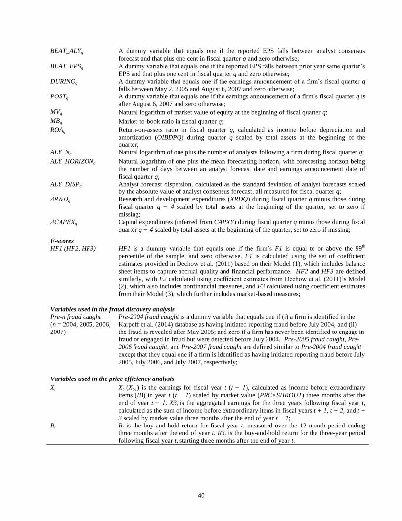
40

BEAT_ALYq A dummy variable that equals one if the reported EPS falls between analyst consensus

forecast and that plus one cent in fiscal quarter q and zero otherwise;

BEAT_EPSq A dummy variable that equals one if the reported EPS falls between prior year same quarter’s

EPS and that plus one cent in fiscal quarter q and zero otherwise;

DURINGq A dummy variable that equals one if the earnings announcement of a firm’s fiscal quarter q

falls between May 2, 2005 and August 6, 2007 and zero otherwise;

POSTq A dummy variable that equals one if the earnings announcement of a firm’s fiscal quarter q is

after August 6, 2007 and zero otherwise;

MVq Natural logarithm of market value of equity at the beginning of fiscal quarter q;

MBq Market-to-book ratio in fiscal quarter q;

ROAq Return-on-assets ratio in fiscal quarter q, calculated as income before depreciation and

amortization (OIBDPQ) during quarter q scaled by total assets at the beginning of the

quarter;

ALY_Nq Natural logarithm of one plus the number of analysts following a firm during fiscal quarter q;

ALY_HORIZONq Natural logarithm of one plus the mean forecasting horizon, with forecasting horizon being

the number of days between an analyst forecast date and earnings announcement date of

fiscal quarter q;

ALY_DISPq Analyst forecast dispersion, calculated as the standard deviation of analyst forecasts scaled

by the absolute value of analyst consensus forecast, all measured for fiscal quarter q;

ΔR&Dq Research and development expenditures (XRDQ) during fiscal quarter q minus those during

fiscal quarter q − 4 scaled by total assets at the beginning of the quarter, set to zero if

missing;

ΔCAPEXq Capital expenditures (inferred from CAPXY) during fiscal quarter q minus those during fiscal

quarter q − 4 scaled by total assets at the beginning of the quarter, set to zero if missing;

F-scores HF1 (HF2, HF3) HF1 is a dummy variable that equals one if the firm’s F1 is equal to or above the 99

th

percentile of the sample, and zero otherwise. F1 is calculated using the set of coefficient

estimates provided in Dechow et al. (2011) based on their Model (1), which includes balance

sheet items to capture accrual quality and financial performance. HF2 and HF3 are defined

similarly, with F2 calculated using coefficient estimates from Dechow et al. (2011)’s Model

(2), which also includes nonfinancial measures, and F3 calculated using coefficient estimates

from their Model (3), which further includes market-based measures;

Variables used in the fraud discovery analysis Pre-n fraud caught

(n = 2004, 2005, 2006,

2007)

Pre-2004 fraud caught is a dummy variable that equals one if (i) a firm is identified in the

Karpoff et al. (2014) database as having initiated reporting fraud before July 2004, and (ii)

the fraud is revealed after May 2005; and zero if a firm has never been identified to engage in

fraud or engaged in fraud but were detected before July 2004. Pre-2005 fraud caught, Pre-

2006 fraud caught, and Pre-2007 fraud caught are defined similar to Pre-2004 fraud caught

except that they equal one if a firm is identified as having initiated reporting fraud before July

2005, July 2006, and July 2007, respectively;

Variables used in the price efficiency analysis

Xt Xt (Xt-1) is the earnings for fiscal year t (t − 1), calculated as income before extraordinary

items (IB) in year t (t − 1) scaled by market value (PRC×SHROUT) three months after the

end of year t − 1. X3t is the aggregated earnings for the three years following fiscal year t,

calculated as the sum of income before extraordinary items in fiscal years t + 1, t + 2, and t +

3 scaled by market value three months after the end of year t − 1;

Rt Rt is the buy-and-hold return for fiscal year t, measured over the 12-month period ending

three months after the end of year t. R3t is the buy-and-hold return for the three-year period

following fiscal year t, starting three months after the end of year t.

41

Table 1: Firm characteristics of the treatment group and control group in the fiscal year of 2003

Panel A: Treatment group and control group drawn from the 2004 Russell 3000 index, balanced panel sample This panel reports summary statistics of the firm characteristics for the balanced panel sample of the treatment and control groups measured in 2003, the year

immediately before the Regulation SHO’s pilot program was announced. The sample is drawn from the 2004 Russell 3000 index and requires a firm to have data

available to calculate firm characteristics and discretionary accruals across the entire sample period used in the empirical tests (i.e., 2001-2003, and 2005-2010).

A firm is classified into the treatment group if its stock is designated as a pilot stock and into the control group otherwise. Variable definitions are listed in

Appendix A. All variables are winsorized at the 1% and 99% levels. ASSET is in millions of dollars. ASSETGR, CAPEX, R&D, ROA, CFO, LEV, CASH, and

DIVIDENDS are in percentage points. ***, **, and * indicate significance at the 1%, 5%, and 10% levels using two-tailed tests.

Treatment Group (PILOT = 1) Control Group (PILOT = 0) Tests for differences

Variable N Mean Median Std. Dev N Mean Median Std. Dev t-statistic

Wilcoxon z-

statistic

ASSET 388 3,748.61 817.69 8,512.30 709 3,746.25 817.42 8,647.29 0.00 0.51

MB 388 2.75 1.95 3.79 709 2.60 1.98 3.13 0.68 0.03

ASSETGR 388 13.42 7.88 31.28 709 13.22 7.66 30.18 0.10 -0.30

CAPEX 388 5.55 3.76 5.54 709 5.50 3.65 5.88 0.14 0.91

R&D 388 4.19 0.00 8.40 709 4.04 0.32 7.83 0.27 -0.94

ROA 388 14.37 14.51 12.70 709 14.15 14.29 14.30 0.25 0.22

CFO 388 11.36 11.33 10.68 709 10.56 10.46 13.26 1.10 1.10

LEV 388 29.36 26.46 27.50 709 29.80 27.56 28.25 -0.25 -0.24

CASH 388 0.21 0.12 0.26 709 0.22 0.11 0.28 -0.44 -0.32

DIVIDENDS 388 0.83 0.00 1.49 709 0.73 0.00 1.33 1.14 1.07

42

Table 1 (continued)

Panel B: Treatment group and control group drawn from the 2004 Russell 3000 index, unbalanced panel sample This panel reports summary statistics of the firm characteristics for the unbalanced panel sample of the treatment and control groups measured in 2003, the year

immediately before the Regulation SHO’s pilot program was announced. The sample is drawn from the 2004 Russell 3000 index and requires a firm to have data

available to calculate a given firm characteristic in a given year. A firm is classified into the treatment group if its stock is designated as a pilot stock and into the

control group otherwise. Variable definitions are listed in Appendix A. All variables are winsorized at the 1% and 99% levels. ASSET is in millions of dollars.

ASSETGR, CAPEX, R&D, ROA, CFO, LEV, CASH, and DIVIDENDS are in percentage points. ***, **, and * indicate significance at the 1%, 5%, and 10% levels

using two-tailed tests.

Treatment Group (PILOT = 1) Control Group (PILOT = 0)

Tests for differences

Variable N Mean Median Std. Dev N Mean Median Std. Dev t-statistic

Wilcoxon z-

statistic

ASSET 782 2,918.37 726.92 7,471.08 1,610 2,941.31 669.22 7,883.20 -0.07 1.26

MB 759 2.66 1.89 3.84 1,534 2.55 1.85 4.15 0.60 1.05

ASSETGR 781 17.81 8.82 40.64 1,605 17.61 8.45 43.10 0.11 0.38

CAPEX 741 5.59 3.61 6.21 1,504 5.28 3.31 5.98 1.13 1.74*

R&D 781 5.78 0.00 11.96 1,605 6.10 0.22 12.22 -0.61 -1.06

ROA 778 10.67 12.79 18.92 1,604 9.68 11.87 20.88 1.15 1.23

CFO 742 8.19 9.88 17.20 1,505 7.20 9.24 19.20 1.23 1.39

LEV 781 30.82 28.06 29.18 1,602 31.54 27.27 31.21 -0.55 0.11

CASH 781 0.27 0.13 0.36 1,605 0.27 0.12 0.38 -0.48 -0.66

DIVIDENDS 778 0.73 0.00 1.55 1,600 0.77 0.00 1.65 -0.69 -1.13

43

Table 2: Discretionary accruals before, during, and after the pilot program, univariate difference-in-differences tests The top half of Panel A reports summary statistics of the level of discretionary accruals for the balanced panel sample of the treatment and control groups for the

three-year periods before, during, and after the Regulation SHO’s pilot program, and the differences in the mean and/or median. The bottom half of Panel A

reports the univariate results of difference-in-differences (DiD) tests, with standard errors reported in parentheses below the DiD estimators. The sample is drawn

from the 2004 Russell 3000 index and requires a firm to have data available to calculate firm characteristics and discretionary accruals across the entire sample

period (i.e., 2001-2003, and 2005-2010). A firm is classified into the treatment group if its stock is designated as pilot stock during the program and into the

control group otherwise. Panel B reports summary statistics of the level of discretionary accruals for the unbalanced panel sample of the treatment and control

groups. The sample is also drawn from the 2004 Russell 3000 index and but only requires a firm to have data available to calculate discretionary accruals in a

given year. Variables definitions are provided in Appendix A. ***, **, and * indicate significance at the 1%, 5%, and 10% levels using two-tailed tests.

Panel A: Balanced Panel Sample

Treatment Group (PILOT = 1)

Control Group (PILOT = 0)

Cross-sectional estimator:

Variable of interest N Mean Median N Mean Median

Difference

in Mean

Difference

in Median

Discretionary accruals

PRE (2001-2003) 1,164 -0.004 -0.001 2,127 -0.004 -0.003 -0.001 0.002

DURING (2005-2007) 1,164 -0.014 -0.012 2,127 -0.004 -0.004 -0.011** -0.008**

POST (2008-2010) 1,164 0.000 0.000 2,127 -0.003 -0.001 0.004 0.001

Univariate DiD test N

Time-series

estimator N

Time-series

estimator

DiD

estimator

t-statistic

of DiD estimator

ΔDiscretionary accruals

DURING-PRE 388 -0.011** 709 0.000 -0.011

(0.006) -1.67*

POST-DURING 388 0.013*** 709 0.001 0.013

(0.006) 2.06**

POST-PRE 388 0.003 709 0.001 0.002

(0.006) 0.32

Panel B: Unbalanced Panel Sample

Treatment Group (PILOT = 1)

Control Group (PILOT = 0)

Cross-sectional estimator:

Variable of interest N Mean Median N Mean Median

Difference

in Mean

Difference

in Median

Discretionary accruals

PRE (2001-2003) 2,067 -0.002 0.000 4,151 0.000 -0.002 -0.002 0.002

DURING (2005-2007) 1,865 -0.012 -0.009 3,740 -0.003 -0.003 -0.009** -0.006**

POST (2008-2010) 1,605 0.001 0.001 3,087 -0.005 -0.003 0.006 0.004

44

Table 3: Multivariate difference-in-differences tests: discretionary accruals This table reports the ordinary least squares (OLS) regression results that estimate differences in pilot and non-pilot

firms’ discretionary accruals for the periods before, during, and after Regulation SHO’s pilot program, using a

balanced panel sample. The sample is drawn from the 2004 Russell 3000 index and requires a firm to have data

available to calculate firm characteristics and discretionary accruals across the entire sample period (i.e., 2001-2003,

and 2005-2010). A firm is classified into the treatment group if its stock is designated as a pilot stock during the

program and into the control group otherwise. We estimate the following model: Discretionary accrualsi,t = β0 +

β1PILOTi×DURINGt + β2PILOTi×POSTt + β3PILOTi + β4DURINGt + β5POSTt + εi,t in Column (1). We then

augment the model by including SIZE, MB, ROA, and LEV in Column (2) and by further including eight year fixed

effects from 2002-2003, and from 2005-2010 in Column (3). We omit PILOT and POST in Column (3) to avoid

multicollinearity. Variable definitions are provided in Appendix A. Coefficient estimates are shown in bold and

their standard errors clustered by year and firm are displayed in parentheses below. For brevity, the coefficient

estimates on year fixed effects in Column (3) are not reported. ***, **, and * indicate significance at the 1%, 5%, and

10% levels using two-tailed tests.

(1) (2) (3)

Dependent Variable Discretionary accruals

PILOT×DURING -0.010** -0.010** -0.010**

(0.004) (0.004) (0.004)

PILOT×POST 0.004 0.003 0.003

(0.004) (0.004) (0.005)

PILOT -0.000 0.000 0.000

(0.003) (0.003) (0.003)

DURING -0.001 -0.001

(0.002) (0.002)

POST 0.000 -0.001

(0.005) (0.005)

SIZE 0.002* 0.002*

(0.001) (0.001)

MB -0.001 -0.001

(0.001) (0.001)

ROA -0.041** -0.041***

(0.016) (0.016)

LEV -0.014 -0.013

(0.009) (0.008)

INTERCEPT -0.004** -0.006 -0.006

(0.002) (0.007) (0.008)

Year fixed effects Included

# of obs. 9,873 9,873 9,873

Adjusted R2 0.10% 0.40% 0.40%

45

Table 4: Multivariate difference-in-differences tests: firm’s likelihood of beating earnings targets This table reports the probit regression results that estimate differences in pilot and non-pilot firms’ likelihood of

meeting or marginally beating the quarterly analyst consensus forecast (or the reported earnings of same quarter last

year) for the periods before, during, and after Regulation SHO’s pilot program. The sample is drawn from the 2004

Russell 3000 index and requires a firm to have data available for analyst forecast related variables (or reported EPS

of same quarter last year), and controls during the sample period (i.e., 2001-2003, and 2005-2010). A firm is

classified into the treatment group if its stock is designated as a pilot stock during the program and into the control

group otherwise. We estimate the following model: BEAT_ALY (BEAT_EPS)i,q = β0 + β1PILOTi×DURINGq +

β2PILOTi×POSTq + β3PILOTi + β4DURINGq + β5POSTq + εi,q in Column (1) (Column (3)). We then augment the

model by including controls in Columns (2) and (4). Variables definitions are provided in Appendix A. Coefficient

estimates are shown in bold and their standard errors clustered by quarter end and firm are displayed in parentheses

below. For brevity, the coefficient estimates on quarter end fixed effects are not reported. ***, **, and * indicate

significance at the 1%, 5%, and 10% levels using two-tailed tests.

(1) (2) (3) (4)

Dependent Variables BEAT_ALY BEAT_EPS

PILOT×DURING -0.081** -0.079** -0.077* -0.078*

(0.040) (0.040) (0.043) (0.044)

PILOT×POST 0.019 0.016 0.005 0.001

(0.043) (0.042) (0.032) (0.032)

PILOT 0.025 0.019 0.041* 0.046*

(0.027) (0.028) (0.023) (0.023)

DURING 0.240*** 0.249*** -0.128 -0.114

(0.039) (0.050) (0.173) (0.188)

POST -0.002 -0.109 0.138 -0.040

(0.163) (0.129) (0.215) (0.257)

MV -0.002 -0.065***

(0.010) (0.007)

MB 0.018*** 0.006**

(0.003) (0.003)

ROA -0.407 1.393***

(0.426) (0.315)

ALY_N 0.000

(0.022)

ALY_HORIZON -0.034**

(0.015)

ALY_DISP -0.196***

(0.040)

ΔR&D -1.802** -0.255

(0.896) (0.454)

ΔCAPEX 0.133 0.373

(0.916) (0.389)

INTERCEPT -0.741*** -0.693*** -1.530*** -0.872***

(0.013) (0.067) (0.214) (0.271)

Quarter fixed effects Included Included Included Included

# of obs. 28,626 28,341 59,830 59,573

Pseudo R2 3.40% 3.40% 0.99% 1.46%

46

Table 5: Multivariate difference-in-differences tests: the likelihood of misstating based on F-scores This table reports the probit regression results that estimate differences in pilot and non-pilot firms’ likelihood of

being classified as misstating based on F-scores of Dechow et al. (2011) for the periods before, during, and after

Regulation SHO’s pilot program. The sample is drawn from the 2004 Russell 3000 index and requires a firm to have

data available to calculate F-scores and controls during the sample period (i.e., 2001-2003, and 2005-2010). A firm

is classified into the treatment group if its stock is designated as a pilot stock during the program and into the control

group otherwise. We estimate the following model: HF1 (HF2, HF3)i,t = β0 + β1PILOTi×DURINGt +

β2PILOTi×POSTt + β3PILOTi + β4DURINGt + β5POSTt + εi,t in Columns (1), (3), and (5). We then augment the

model by including SIZE, MB, ROA, and LEV in Columns (2), (4), and (6). Variables definitions are provided in

Appendix A. Coefficient estimates are shown in bold and their standard errors clustered by year and firm are

displayed in parentheses below. ***, **, and * indicate significance at the 1%, 5%, and 10% levels using two-tailed

tests.

(1) (2) (3) (4) (5) (6)

Dependent Variables HF1 HF2 HF3

PILOT×DURING -0.178** -0.174** -0.189** -0.187** -0.200** -0.196**

(0.080) (0.081) (0.079) (0.080) (0.080) (0.081)

PILOT×POST -0.177** -0.170* -0.186** -0.181** -0.169** -0.167*

(0.087) (0.088) (0.087) (0.088) (0.086) (0.087)

PILOT -0.001 -0.011 -0.006 -0.016 -0.004 -0.012

(0.035) (0.036) (0.036) (0.036) (0.038) (0.039)

DURING -0.976*** -1.024*** -0.942*** -0.989*** -0.974*** -1.015***

(0.046) (0.047) (0.045) (0.046) (0.046) (0.046)

POST -0.941*** -0.989*** -0.928*** -0.977*** -0.887*** -0.939***

(0.049) (0.050) (0.048) (0.050) (0.048) (0.049)

SIZE 0.079*** 0.084*** 0.072***

(0.017) (0.017) (0.017)

MB 0.021*** 0.020*** 0.014**

(0.006) (0.006) (0.006)

ROA 0.093 -0.000 0.026

(0.168) (0.167) (0.170)

LEV 0.127 0.108 0.294***

(0.084) (0.083) (0.088)

INTERCEPT -0.081*** -0.735*** -0.063*** -0.726*** -0.004 -0.628***

(0.021) (0.111) (0.022) (0.110) (0.023) (0.111)

# of obs. 9,871 9,871 9,871 9,871 9,871 9,871

Pseudo R2 11.5% 12.5% 11.0% 12.1% 10.8% 12.0%

47

Table 6: Multivariate difference-in-differences tests, controlling for investment This table reports the OLS regression results that estimate differences in pilot and non-pilot firms’ discretionary

accruals for the periods before, during, and after Regulation SHO’s pilot program, using a balanced panel sample.

The sample is drawn from the 2004 Russell 3000 index and requires a firm to have data available to calculate firm

characteristics and discretionary accruals across the entire sample period (i.e., 2001-2003, and 2005-2010). A firm is

classified into the treatment group if its stock is designated as a pilot stock during the program and into the control

group otherwise. We estimate the following model: Discretionary accrualsi,t = β0 + β1PILOTi×DURINGt +

β2PILOTi×POSTt + β3PILOTi + β4DURINGt + β5POSTt + β6SIZEi,t + β7MBi,t + β8ROAi,t + β9LEVi,t + εi,t. We

include R&D and CAPEX in Column (1), INVESTMENT in Column (2), and further include their squared terms in

Columns (3)-(4). In Column (5), we replace the dependent variable Discretionary accruals with Discretionary

accruals_MBadj. Variable definitions are provided in Appendix A. Coefficient estimates are shown in bold and their

standard errors clustered by year and firm are displayed in parentheses below. ***, **, and * indicate significance at the

1%, 5%, and 10% levels using two-tailed tests.

(1) (2) (3) (4) (5)

Dependent Variables Discretionary accruals

Discretionary

accruals_MBadj

PILOT×DURING -0.010** -0.010** -0.010** -0.010** -0.018***

(0.004) (0.004) (0.004) (0.004) (0.004)

PILOT×POST 0.003 0.003 0.003 0.003 0.004

(0.005) (0.004) (0.005) (0.004) (0.006)

PILOT -0.000 -0.000 -0.000 -0.000 0.004

(0.003) (0.003) (0.003) (0.003) (0.003)

DURING -0.001 -0.001 -0.001 -0.001 0.002

(0.002) (0.001) (0.002) (0.001) (0.002)

POST -0.002 -0.003 -0.002 -0.003 0.001

(0.005) (0.005) (0.005) (0.005) (0.005)

SIZE 0.001 0.001 0.001 0.001 0.001

(0.001) (0.001) (0.001) (0.001) (0.001)

MB -0.000 -0.000 -0.000 -0.000 -0.001

(0.001) (0.001) (0.001) (0.001) (0.001)

ROA -0.062*** -0.053*** -0.064*** -0.058*** -0.044**

(0.014) (0.015) (0.014) (0.015) (0.019)

LEV -0.017** -0.016* -0.016* -0.015* -0.013

(0.009) (0.008) (0.009) (0.009) (0.009)

R&D -0.001*** -0.001*

(0.000) (0.000)

CAPEX -0.001*** -0.001**

(0.000) (0.000)

INVESTMENT -0.001*** -0.001**

(0.000) (0.000)

R&D2 -0.000

(0.000)

CAPEX2 0.000

(0.000)

INVESTMENT2 -0.000

(0.000)

INTERCEPT 0.015* 0.013* 0.013* 0.010 -0.001

(0.008) (0.008) (0.008) (0.007) (0.009)

# of obs. 9,849 9,873 9,873 9,873 9,206

Adjusted R2 1.06% 1.02% 1.10% 1.10% 0.50%

48

Table 7: Multivariate difference-in-differences tests, partitioned on seasoned equity offering This table reports the OLS regression results that estimate differences in pilot and non-pilot firms’ discretionary

accruals for the periods before, during, and after Regulation SHO’s pilot program, separately for the subsample of

equity issuers and the subsample of non-equity-issuers. The sample is drawn from the 2004 Russell 3000 index and

requires a firm to have data available to calculate firm characteristics and discretionary accruals across the entire

sample period (i.e., 2001-2003, and 2005-2010). On the left panel of the table, we define a firm as an Equity Issuer

if the firm issued equity at least once during the two prior fiscal years, as recorded in the Thomson Reuters

Securities Data Company (SDC) Platinum database, and Non-Equity-Issuer otherwise. On the right panel of the

table, we define a firm as an Equity Issuer if the firm issued equity at least once during a given fiscal year, as

recorded in the Thomson Reuters Securities Data Company (SDC) Platinum database, and Non-Equity-Issuer

otherwise. A firm is classified into the treatment group if its stock is designated as a pilot stock during the program

and into the control group otherwise. We estimate the following model: Discretionary accrualsi,t = β0 +

β1PILOTi×DURINGt + β2PILOTi×POSTt + β3PILOTi + β4DURINGt + β5POSTt + εi,t in Columns (1), (3), (5), and

(7). We then augment the model by including SIZE, MB, ROA, and LEV in Columns (2), (4), (6), and (8). Variable

definitions are provided in Appendix A. Coefficient estimates are shown in bold and their standard errors clustered

by year and firm are displayed in parentheses below. ***, **, and * indicate significance at the 1%, 5%, and 10% levels

using two-tailed tests.

(1) (2) (3) (4) (5) (6) (7) (8)

Partition based on past equity issuance Partition based on current equity issuance

Equity Issuers Non-Equity-Issuers Equity Issuers Non-Equity-Issuers

Dependent Variable Discretionary accruals Discretionary accruals

PILOT×DURING 0.004 0.006 -0.011** -0.012** -0.027 -0.020 -0.009*** -0.010***

(0.008) (0.008) (0.005) (0.005) (0.036) (0.038) (0.003) (0.003)

PILOT×POST -0.036 -0.035 0.007 0.006 0.007 0.006 0.003 0.003

(0.028) (0.028) (0.005) (0.005) (0.052) (0.052) (0.006) (0.006)

PILOT 0.003 0.003 -0.001 -0.001 -0.016 -0.016 0.001 0.002

(0.006) (0.006) (0.004) (0.004) (0.012) (0.012) (0.002) (0.002)

DURING -0.001 -0.002 -0.001 -0.002 -0.002 -0.009 0.000 -0.000

(0.010) (0.010) (0.002) (0.003) (0.036) (0.038) (0.001) (0.002)

POST 0.013** 0.011 -0.001 -0.003 -0.005 -0.011 0.001 0.000

(0.006) (0.009) (0.006) (0.006) (0.014) (0.016) (0.006) (0.006)

SIZE -0.002 0.002** -0.001 0.002**

(0.002) (0.001) (0.005) (0.001)

MB -0.002 -0.000 -0.002 -0.001

(0.001) (0.001) (0.002) (0.001)

ROA -0.021 -0.049*** -0.040 -0.041*

(0.040) (0.019) (0.048) (0.021)

LEV 0.005 -0.016** 0.016 -0.016

(0.018) (0.008) (0.018) (0.010)

INTERCEPT -0.010 0.009** -0.002 -0.005 0.011** 0.023 -0.005*** -0.008

(0.009) (0.004) (0.003) (0.008) (0.004) (0.030) (0.001) (0.007)

# of obs. 1,199 1,199 8,674 8,674 559 559 9,314 9,314

Adjusted R2 0.20% 0.60% 0.10% 0.40% 0.70% 1.40% 0.10% 0.30%

49

Table 8: The effect of pilot program on the discovery of financial misrepresentation This table reports the probit regression results that estimate differences in pilot and non-pilot firms’ likelihood of

being identified as having engaged in fraud in the Karpoff et al. (2014) database. The sample is drawn from the 2004

Russell 3000 index. A firm is classified into the treatment group if its stock is designated as a pilot stock during the

program and into the control group otherwise. We estimate the following model: Pre-2004 fraud caughti = β0 +

β1PILOTi + εi in Column (1). We then augment the model by including MV, MB in Column (2). We estimate Pre-

2005 fraud caught (Pre-2006 fraud caught, Pre-2007 fraud caught)i = β0 + β1PILOTi + β2MVi + β3MBi + εi in

Columns (3)-(5). MV and MB are the log of market capitalization and the market-to-book ratio of the firm at the

end of fiscal year 2003. Other variable definitions are provided in Appendix A. Coefficient estimates are shown in

bold and their standard errors clustered by year and firm are displayed in parentheses below. ***, **, and * indicate

significance at the 1%, 5%, and 10% levels using two-tailed tests.

(1) (2) (3) (4) (5)

Dependent Variables

Pre-2004

fraud caught

Pre-2004

fraud caught

Pre-2005

fraud caught

Pre-2006

fraud caught

Pre-2007

fraud caught

PILOT 0.202*** 0.201*** 0.189*** 0.182** 0.141*

(0.066) (0.063) (0.065) (0.073) (0.077)

MV 0.067** 0.058** 0.055* 0.059**

(0.027) (0.029) (0.028) (0.023)

MB -0.018 -0.003 -0.003 -0.004

(0.012) (0.013) (0.012) (0.012)

INTERCEPT -2.078*** -2.511*** -2.482*** -2.456*** -2.467***

(0.027) (0.196) (0.207) (0.197) (0.160)

Industry Fixed Effect Included Included Included Included Included

# of obs. 2,764 2,705 2,708 2,711 2,715

Pseudo R2 4.94% 5.41% 5.27% 4.69% 4.07%

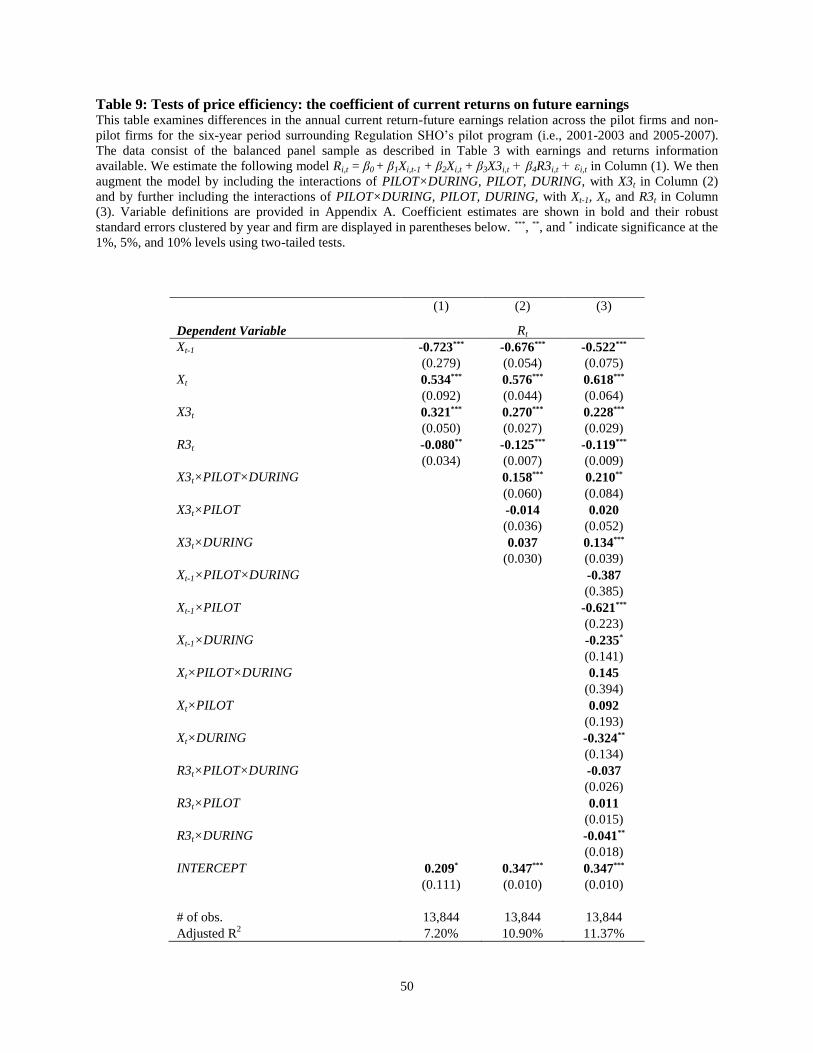
50

Table 9: Tests of price efficiency: the coefficient of current returns on future earnings This table examines differences in the annual current return-future earnings relation across the pilot firms and non-

pilot firms for the six-year period surrounding Regulation SHO’s pilot program (i.e., 2001-2003 and 2005-2007).

The data consist of the balanced panel sample as described in Table 3 with earnings and returns information

available. We estimate the following model Ri,t = β0 + β1Xi,t-1 + β2Xi,t + β3X3i,t + β4R3i,t + εi,t in Column (1). We then

augment the model by including the interactions of PILOT×DURING, PILOT, DURING, with X3t in Column (2)

and by further including the interactions of PILOT×DURING, PILOT, DURING, with Xt-1, Xt, and R3t in Column

(3). Variable definitions are provided in Appendix A. Coefficient estimates are shown in bold and their robust

standard errors clustered by year and firm are displayed in parentheses below. ***, **, and * indicate significance at the

1%, 5%, and 10% levels using two-tailed tests.

(1) (2) (3)

Dependent Variable Rt

Xt-1 -0.723*** -0.676*** -0.522***

(0.279) (0.054) (0.075)

Xt 0.534*** 0.576*** 0.618***

(0.092) (0.044) (0.064)

X3t 0.321*** 0.270*** 0.228***

(0.050) (0.027) (0.029)

R3t -0.080** -0.125*** -0.119***

(0.034) (0.007) (0.009)

X3t×PILOT×DURING 0.158*** 0.210**

(0.060) (0.084)

X3t×PILOT -0.014 0.020

(0.036) (0.052)

X3t×DURING 0.037 0.134***

(0.030) (0.039)

Xt-1×PILOT×DURING -0.387

(0.385)

Xt-1×PILOT -0.621***

(0.223)

Xt-1×DURING -0.235*

(0.141)

Xt×PILOT×DURING 0.145

(0.394)

Xt×PILOT 0.092

(0.193)

Xt×DURING -0.324**

(0.134)

R3t×PILOT×DURING -0.037

(0.026)

R3t×PILOT 0.011

(0.015)

R3t×DURING -0.041**

(0.018)

INTERCEPT 0.209* 0.347*** 0.347***

(0.111) (0.010) (0.010)

# of obs. 13,844 13,844 13,844

Adjusted R2 7.20% 10.90% 11.37%

51

Table 10: Tests of price efficiency: post-earnings announcement drift (PEAD) This table reports differences in the post-earnings announcement drift across the pilot firms and non-pilot firms for

the three-year period during Regulation SHO’s pilot program (i.e., 2005-2007). The data consist of the balanced

panel sample as described in Table 3 with earnings, analyst forecasts, and return information available. In each

quarter, the sample firms are sorted into ten deciles (D1-D10) based on their earnings surprises. The earnings

surprise is calculated as the firm’s actual earnings per share (EPS) minus the latest analyst consensus EPS forecast

before the earnings announcement date (both from I/B/E/S), scaled by the firm’s stock price two days before the

earnings announcement date. PEAD is the cumulative abnormal return (CAR) following the earnings surprise,

calculated as the stock’s raw return minus the corresponding value-weighted market return over the (+2, +11)

window relative to the earnings announcement date. ***, **, and * indicate significance at the 1%, 5%, and 10% levels

using two-tailed tests.

Post-earnings announcement drift (+2, +11)

Treatment Group

Control Group

t-Statistics

Treatment - Control

Earnings surprise

D1 (Most negative) -0.38% -1.26%*** 2.47**

D2 -0.41%** -0.41%*** 0.01

D3 -0.38%** -0.57%*** 0.88

D4 0.00% -0.07% 0.35

D5 -0.22% -0.24%** 0.12

D6 -0.13% -0.16% 0.13

D7 0.10% -0.10% 0.95

D8 -0.02% -0.06% 0.16

D9 0.23% 0.36%** -0.45

D10 (Most positive) 0.97%*** 0.83%*** 0.43

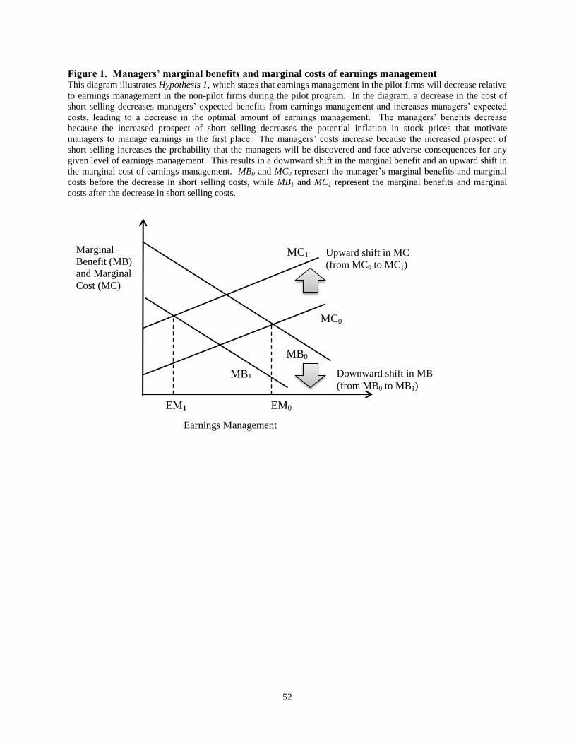
52

Figure 1. Managers’ marginal benefits and marginal costs of earnings management This diagram illustrates Hypothesis 1, which states that earnings management in the pilot firms will decrease relative

to earnings management in the non-pilot firms during the pilot program. In the diagram, a decrease in the cost of

short selling decreases managers’ expected benefits from earnings management and increases managers’ expected

costs, leading to a decrease in the optimal amount of earnings management. The managers’ benefits decrease

because the increased prospect of short selling decreases the potential inflation in stock prices that motivate

managers to manage earnings in the first place. The managers’ costs increase because the increased prospect of

short selling increases the probability that the managers will be discovered and face adverse consequences for any

given level of earnings management. This results in a downward shift in the marginal benefit and an upward shift in

the marginal cost of earnings management. MB0 and MC0 represent the manager’s marginal benefits and marginal

costs before the decrease in short selling costs, while MB1 and MC1 represent the marginal benefits and marginal

costs after the decrease in short selling costs.

MC1

MC0

MB1

MB0

Marginal

Benefit (MB)

and Marginal

Cost (MC)

Earnings Management

EM0 EM1

Upward shift in MC

(from MC0 to MC1)

Downward shift in MB

(from MB0 to MB1)

53

Figure 2. Discretionary accruals for pilot vs. non-pilot firms This figure displays the results reported in Panel A of Table 2. It depicts the mean discretionary accruals for the

balanced panel sample of the treatment group and control group for the periods before, during, and after Regulation

SHO’s pilot program, i.e., 2001-2003, 2005-2007, and 2008-2010. The sample is drawn from the 2004 Russell 3000

index and requires a firm to have data available to calculate firm characteristics and discretionary accruals across the

entire sample period used in the empirical tests (i.e., 2001-2003, and 2005-2010).

-0.016

-0.014

-0.012

-0.010

-0.008

-0.006

-0.004

-0.002

0.000

0.002

Pre-pilot During-pilot Post-Pilot

Discretionary Accruals of Pilot Firms

Discretionary Accruals of Non-pilot Firms