Is Accounting an Information Science?

John Felllingham

Ohio State University

Haijin Lin

University of Houston

2017

Abstract: The central result is an equality connecting accounting numbers

with information. ln(1 + income

assets

)= rf + I (X;Y ), rf is the risk free rate, ln

is the natural logarithm, and I(X;Y ) is a Shannon information measure. The

equality is derived using economic income accounting; it is shown to hold, un-

der appropriate conditions, for declining balance and straight line depreciation

methods. Some social welfare implications are explored.

1

Is Accounting an Information Science?

1 Introduction

The paper is a modest attempt at a positive answer to the question about

accounting being an information science. The main result is that accounting

numbers are a statement about how much information the reporting entity has

access to. We do not analyze the communication of the details of the information

available to the reporting entity; the entity conveys a measure of the amount

of information they hold, not the information itself. The metric for amount of

information is Shannon entropy– a function of probabilities (Shannon 1948).

Shannon’s entropy concept has amplified the importance of information, as it

can be treated as a commodity to be accumulated, modified, and transferred;

a commodity as important as energy or mass for descriptive content. Some

other sciences are routinely referred to as "information sciences," physics, for

example, where quantum information is a central idea. Biology, as well, studies

the information content of the genetic code. The title of the paper questions

whether accounting is properly included as a similar and complementary scien-

tific inquiry.

Roughly speaking, the result herein is that the accounting rate of return is

equal to the amount of information possessed by the reporting entity. Account-

ing, then, is a consistent ranking of information systems. As this conclusion

is counter to Blackwell– a general, context free ranking of information systems

does not exist (see Demski 1973)– there must necessarily be some theoretical

restrictions placed upon the environment in which accounting operates. There

are three such restrictions. The first is that the decision maker’s preferences are

distinctly long run in nature. Further, the opportunities available to the deci-

sion maker are characterized by a state-act-payoff matrix and a price vector for

the opportunities. While the state-act-payoff format is not restrictive, there are

some restrictions on the form of the matrix and the price vector. The matrix

must be full rank. Also, the price vector must be free of arbitrage opportunities:

a fairly weak, but nonetheless quite instructive equilibrium condition.

In notation the accounting and information relation is the following:

ln

(1 +

income

assets

)= rf + I (X;Y ) .

2

The left hand side utilizes accounting stocks and flows: income flow is divided

by the stock of assets available for production and investment activities. ln is

the natural logarithm. On the right hand side rf is the risk free rate of return,

and I(X;Y ) is an entropy measure of the increase to the rate of return due to

the availability of information. I (X;Y ) consists entirely of probabilities, and

is, then, free of decision context.

The next section introduces the information numbers as entropy measures.

Section 3 presents conditions under which accounting numbers are connected

with information numbers. The relation is derived in a setting in which ac-

counting is done under the economic income depreciation. The relation is also

derived for declining balance depreciation and straight line depreciation. Sec-

tion 4 confronts what happens when the explicit long run preference assumption

for the decision maker is relaxed, and some speculations about accounting and

social welfare are offered. We conclude in section 5.

2 Information and Rate of Return

2.1 Entropy and mutual information

Shannon entropy is a measure of uncertainty associated with a random variable,

say x. The greater the measure, the larger the uncertainty. The measure is ele-

gantly designed so it is natural to think of the working definition of information

as whatever reduces entropy.

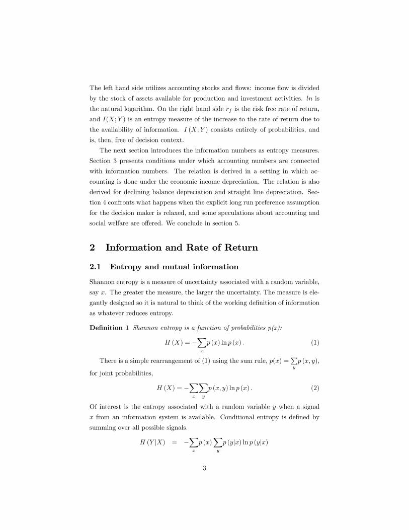
Definition 1 Shannon entropy is a function of probabilities p(x):

H (X) = −∑x

p (x) ln p (x) . (1)

There is a simple rearrangement of (1) using the sum rule, p(x) =∑yp (x, y),

for joint probabilities,

H (X) = −∑x

∑y

p (x, y) ln p (x) . (2)

Of interest is the entropy associated with a random variable y when a signal

x from an information system is available. Conditional entropy is defined by

summing over all possible signals.

H (Y |X) = −∑x

p (x)∑y

p (y|x) ln p (y|x)

3

= −∑x

∑y

p (x, y) ln p (y|x) (3)

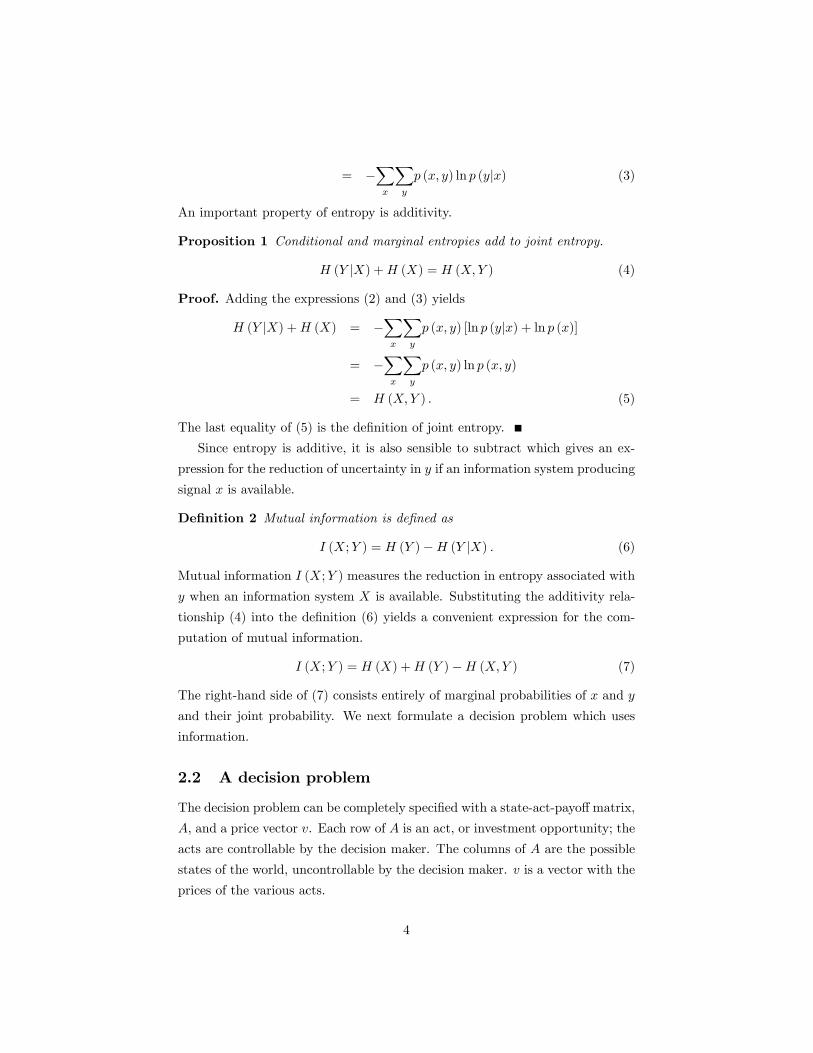
An important property of entropy is additivity.

Proposition 1 Conditional and marginal entropies add to joint entropy.

H (Y |X) +H (X) = H (X,Y ) (4)

Proof. Adding the expressions (2) and (3) yields

H (Y |X) +H (X) = −∑x

∑y

p (x, y) [ln p (y|x) + ln p (x)]

= −∑x

∑y

p (x, y) ln p (x, y)

= H (X,Y ) . (5)

The last equality of (5) is the definition of joint entropy.

Since entropy is additive, it is also sensible to subtract which gives an ex-

pression for the reduction of uncertainty in y if an information system producing

signal x is available.

Definition 2 Mutual information is defined as

I (X;Y ) = H (Y )−H (Y |X) . (6)

Mutual information I (X;Y ) measures the reduction in entropy associated with

y when an information system X is available. Substituting the additivity rela-

tionship (4) into the definition (6) yields a convenient expression for the com-

putation of mutual information.

I (X;Y ) = H (X) +H (Y )−H (X,Y ) (7)

The right-hand side of (7) consists entirely of marginal probabilities of x and y

and their joint probability. We next formulate a decision problem which uses

information.

2.2 A decision problem

The decision problem can be completely specified with a state-act-payoffmatrix,

A, and a price vector v. Each row of A is an act, or investment opportunity; the

acts are controllable by the decision maker. The columns of A are the possible

states of the world, uncontrollable by the decision maker. v is a vector with the

prices of the various acts.

4

Example 1 For a simple example, let A be a 2× 2 matrix with two states and

two acts.

A =

[1 1

1 4

]The first act is a risk-free security which returns a payoff of one in each of the

two states. The second act is a security which pays off one unit in state one and

four in state two. The security prices are denoted in the price vector v.

v =

[1

2

]The state prices, s, solve the linear system

As = v;

and the solution is

s =

[2/3

1/3

].

The payoffs can be framed in scaled Arrow-Debreu format. The acts are

the investments of Arrow-Debreu securities.

Definition 3 An Arrow-Debreu security is one that returns one unit in state i

and zero elsewhere. The price of an Arrow-Debreu security is referred to as the

state price, since it is the amount which must be paid to yield a payoff of one

unit in a particular state.

Scaling sets the price of the security equal to one; the payoffs are scaled

up accordingly. The revised state-act-payoff matrix facing the decision maker,

then, is a diagonal matrix with the scaled payoffs on the diagonal, denoted yi,

equal to 1/si.

act\state state 1 state 2 ... state i

act 1 y1 0 ... 0

act 2 0 y2 ... 0

... ... ... ... 0

act i 0 0 0 yi

(8)

Back to Example 1, the scaled matrix A is written as

A =

[3/2 0

0 3

]

5

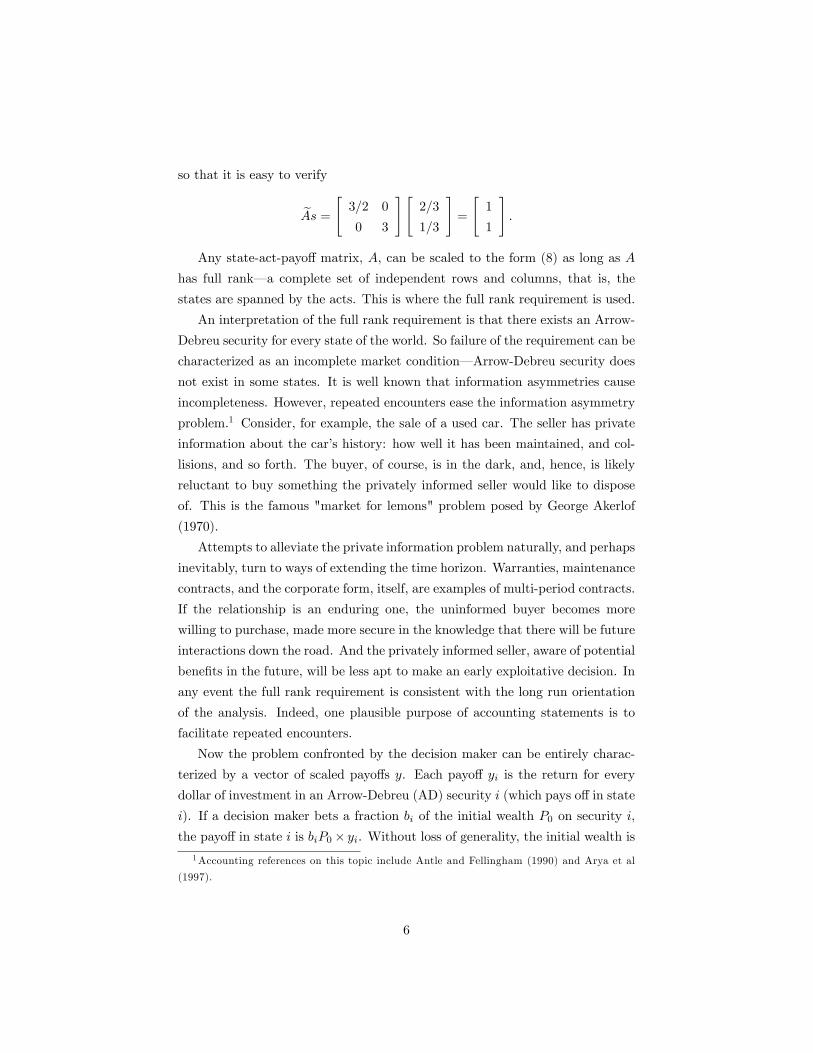
so that it is easy to verify

As =

[3/2 0

0 3

][2/3

1/3

]=

[1

1

].

Any state-act-payoff matrix, A, can be scaled to the form (8) as long as A

has full rank– a complete set of independent rows and columns, that is, the

states are spanned by the acts. This is where the full rank requirement is used.

An interpretation of the full rank requirement is that there exists an Arrow-

Debreu security for every state of the world. So failure of the requirement can be

characterized as an incomplete market condition– Arrow-Debreu security does

not exist in some states. It is well known that information asymmetries cause

incompleteness. However, repeated encounters ease the information asymmetry

problem.1 Consider, for example, the sale of a used car. The seller has private

information about the car’s history: how well it has been maintained, and col-

lisions, and so forth. The buyer, of course, is in the dark, and, hence, is likely

reluctant to buy something the privately informed seller would like to dispose

of. This is the famous "market for lemons" problem posed by George Akerlof

(1970).

Attempts to alleviate the private information problem naturally, and perhaps

inevitably, turn to ways of extending the time horizon. Warranties, maintenance

contracts, and the corporate form, itself, are examples of multi-period contracts.

If the relationship is an enduring one, the uninformed buyer becomes more

willing to purchase, made more secure in the knowledge that there will be future

interactions down the road. And the privately informed seller, aware of potential

benefits in the future, will be less apt to make an early exploitative decision. In

any event the full rank requirement is consistent with the long run orientation

of the analysis. Indeed, one plausible purpose of accounting statements is to

facilitate repeated encounters.

Now the problem confronted by the decision maker can be entirely charac-

terized by a vector of scaled payoffs y. Each payoff yi is the return for every

dollar of investment in an Arrow-Debreu (AD) security i (which pays off in state

i). If a decision maker bets a fraction bi of the initial wealth P0 on security i,

the payoff in state i is biP0× yi. Without loss of generality, the initial wealth is1Accounting references on this topic include Antle and Fellingham (1990) and Arya et al

(1997).

6

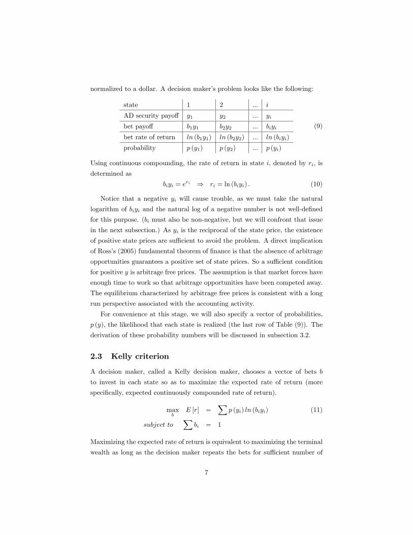
normalized to a dollar. A decision maker’s problem looks like the following:

state 1 2 ... i

AD security payoff y1 y2 ... yi

bet payoff b1y1 b2y2 ... biyi

bet rate of return ln (b1y1) ln (b2y2) ... ln (biyi)

probability p (y1) p (y2) ... p (yi)

(9)

Using continuous compounding, the rate of return in state i, denoted by ri, is

determined as

biyi = eri ⇒ ri = ln (biyi) . (10)

Notice that a negative yi will cause trouble, as we must take the natural

logarithm of biyi and the natural log of a negative number is not well-defined

for this purpose. (bi must also be non-negative, but we will confront that issue

in the next subsection.) As yi is the reciprocal of the state price, the existence

of positive state prices are suffi cient to avoid the problem. A direct implication

of Ross’s (2005) fundamental theorem of finance is that the absence of arbitrage

opportunities guarantees a positive set of state prices. So a suffi cient condition

for positive y is arbitrage free prices. The assumption is that market forces have

enough time to work so that arbitrage opportunities have been competed away.

The equilibrium characterized by arbitrage free prices is consistent with a long

run perspective associated with the accounting activity.

For convenience at this stage, we will also specify a vector of probabilities,

p (y), the likelihood that each state is realized (the last row of Table (9)). The

derivation of these probability numbers will be discussed in subsection 3.2.

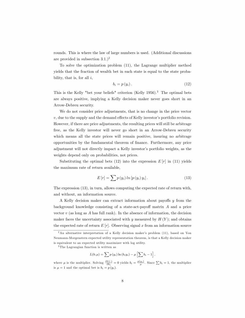
2.3 Kelly criterion

A decision maker, called a Kelly decision maker, chooses a vector of bets b

to invest in each state so as to maximize the expected rate of return (more

specifically, expected continuously compounded rate of return).

maxb

E [r] =∑

p (yi) ln (biyi) (11)

subject to∑

bi = 1

Maximizing the expected rate of return is equivalent to maximizing the terminal

wealth as long as the decision maker repeats the bets for suffi cient number of

7

rounds. This is where the law of large numbers is used. (Additional discussions

are provided in subsection 3.1.)2

To solve the optimization problem (11), the Lagrange multiplier method

yields that the fraction of wealth bet in each state is equal to the state proba-

bility, that is, for all i,

bi = p (yi) . (12)

This is the Kelly "bet your beliefs" criterion (Kelly 1956).3 The optimal bets

are always positive, implying a Kelly decision maker never goes short in an

Arrow-Debreu security.

We do not consider price adjustments, that is no change in the price vector

v, due to the supply and the demand effects of Kelly investor’s portfolio revision.

However, if there are price adjustments, the resulting prices will still be arbitrage

free, as the Kelly investor will never go short in an Arrow-Debreu security

which means all the state prices will remain positive, insuring no arbitrage

opportunities by the fundamental theorem of finance. Furthermore, any price

adjustment will not directly impact a Kelly investor’s portfolio weights, as the

weights depend only on probabilities, not prices.

Substituting the optimal bets (12) into the expression E [r] in (11) yields

the maximum rate of return available,

E [r] =∑

p (yi) ln [p (yi) yi] . (13)

The expression (13), in turn, allows computing the expected rate of return with,

and without, an information source.

A Kelly decision maker can extract information about payoffs y from the

background knowledge consisting of a state-act-payoff matrix A and a price

vector v (as long as A has full rank). In the absence of information, the decision

maker faces the uncertainty associated with y measured by H (Y ); and obtains

the expected rate of return E [r]. Observing signal x from an information source

2An alternative interpretation of a Kelly decision maker’s problem (11), based on Von

Neumann-Morgenstern expected utility representation theorem, is that a Kelly decision maker

is equivalent to an expected utility maximizer with log utility.3The Lagrangian function is written as

L(b;µ) =∑

p (yi) ln (biyi)− µ[∑

bi − 1],

where µ is the multiplier. Solving ∂L(·)∂bi

= 0 yields bi =p(yi)µ. Since

∑bi = 1, the multiplier

is µ = 1 and the optimal bet is bi = p (yi).

8

X, the decision maker faces the uncertainty H (Y |X); and obtains the expected

rate of return E [r|X].4

The following theorem establishes the equivalence relation between the in-

crease of the expected rate of return and the reduction of uncertainty due to

information X.

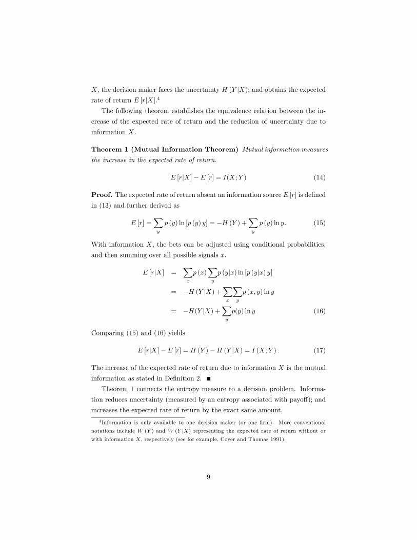
Theorem 1 (Mutual Information Theorem) Mutual information measures

the increase in the expected rate of return.

E [r|X]− E [r] = I(X;Y ) (14)

Proof. The expected rate of return absent an information source E [r] is defined

in (13) and further derived as

E [r] =∑y

p (y) ln [p (y) y] = −H (Y ) +∑y

p (y) ln y. (15)

With information X, the bets can be adjusted using conditional probabilities,

and then summing over all possible signals x.

E [r|X] =∑x

p (x)∑y

p (y|x) ln [p (y|x) y]

= −H (Y |X) +∑x

∑y

p (x, y) ln y

= −H(Y |X) +∑y

p(y) ln y (16)

Comparing (15) and (16) yields

E [r|X]− E [r] = H (Y )−H (Y |X) = I (X;Y ) . (17)

The increase of the expected rate of return due to information X is the mutual

information as stated in Definition 2.

Theorem 1 connects the entropy measure to a decision problem. Informa-

tion reduces uncertainty (measured by an entropy associated with payoff); and

increases the expected rate of return by the exact same amount.

4 Information is only available to one decision maker (or one firm). More conventional

notations include W (Y ) and W (Y |X) representing the expected rate of return without orwith information X, respectively (see for example, Cover and Thomas 1991).

9

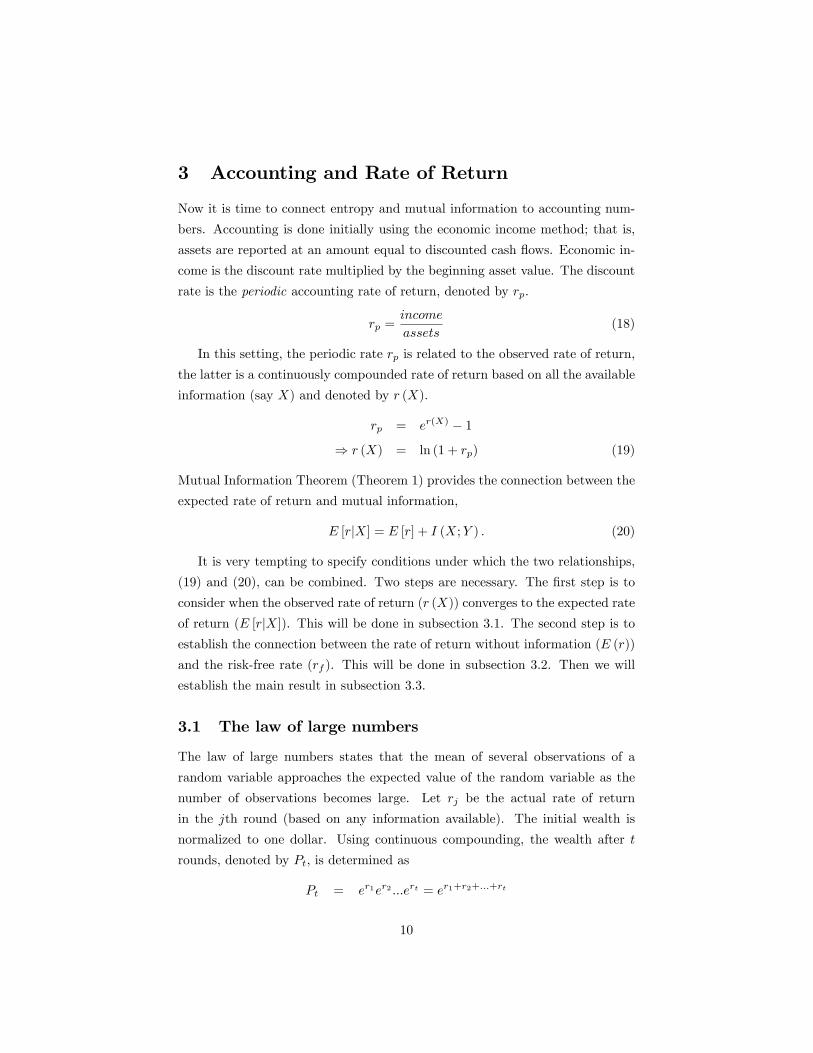
3 Accounting and Rate of Return

Now it is time to connect entropy and mutual information to accounting num-

bers. Accounting is done initially using the economic income method; that is,

assets are reported at an amount equal to discounted cash flows. Economic in-

come is the discount rate multiplied by the beginning asset value. The discount

rate is the periodic accounting rate of return, denoted by rp.

rp =income

assets(18)

In this setting, the periodic rate rp is related to the observed rate of return,

the latter is a continuously compounded rate of return based on all the available

information (say X) and denoted by r (X).

rp = er(X) − 1

⇒ r (X) = ln (1 + rp) (19)

Mutual Information Theorem (Theorem 1) provides the connection between the

expected rate of return and mutual information,

E [r|X] = E [r] + I (X;Y ) . (20)

It is very tempting to specify conditions under which the two relationships,

(19) and (20), can be combined. Two steps are necessary. The first step is to

consider when the observed rate of return (r (X)) converges to the expected rate

of return (E [r|X]). This will be done in subsection 3.1. The second step is to

establish the connection between the rate of return without information (E (r))

and the risk-free rate (rf ). This will be done in subsection 3.2. Then we will

establish the main result in subsection 3.3.

3.1 The law of large numbers

The law of large numbers states that the mean of several observations of a

random variable approaches the expected value of the random variable as the

number of observations becomes large. Let rj be the actual rate of return

in the jth round (based on any information available). The initial wealth is

normalized to one dollar. Using continuous compounding, the wealth after t

rounds, denoted by Pt, is determined as

Pt = er1er2 ...ert = er1+r2+...+rt

10

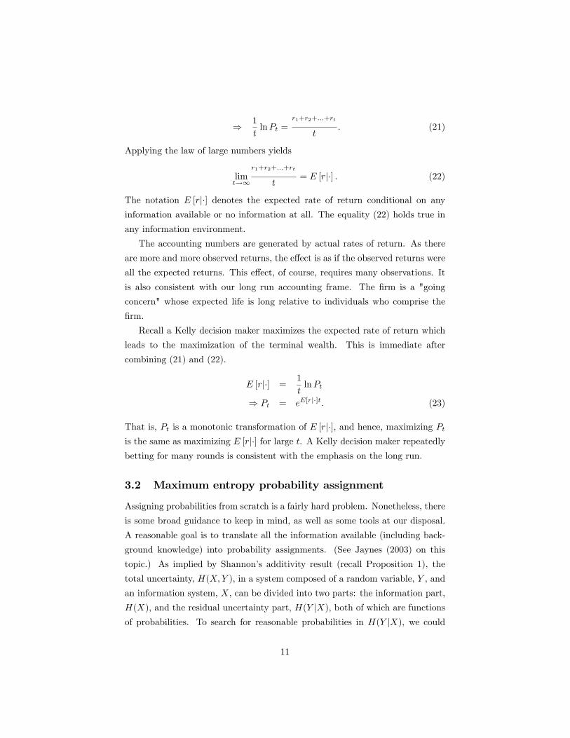
⇒ 1

tlnPt =

r1+r2+...+rt

t. (21)

Applying the law of large numbers yields

limt→∞

r1+r2+...+rt

t= E [r|·] . (22)

The notation E [r|·] denotes the expected rate of return conditional on anyinformation available or no information at all. The equality (22) holds true in

any information environment.

The accounting numbers are generated by actual rates of return. As there

are more and more observed returns, the effect is as if the observed returns were

all the expected returns. This effect, of course, requires many observations. It

is also consistent with our long run accounting frame. The firm is a "going

concern" whose expected life is long relative to individuals who comprise the

firm.

Recall a Kelly decision maker maximizes the expected rate of return which

leads to the maximization of the terminal wealth. This is immediate after

combining (21) and (22).

E [r|·] =1

tlnPt

⇒ Pt = eE[r|·]t. (23)

That is, Pt is a monotonic transformation of E [r|·], and hence, maximizing Ptis the same as maximizing E [r|·] for large t. A Kelly decision maker repeatedlybetting for many rounds is consistent with the emphasis on the long run.

3.2 Maximum entropy probability assignment

Assigning probabilities from scratch is a fairly hard problem. Nonetheless, there

is some broad guidance to keep in mind, as well as some tools at our disposal.

A reasonable goal is to translate all the information available (including back-

ground knowledge) into probability assignments. (See Jaynes (2003) on this

topic.) As implied by Shannon’s additivity result (recall Proposition 1), the

total uncertainty, H(X,Y ), in a system composed of a random variable, Y , and

an information system, X, can be divided into two parts: the information part,

H(X), and the residual uncertainty part, H(Y |X), both of which are functions

of probabilities. To search for reasonable probabilities in H(Y |X), we could

11

proceed in two ways: (i) we could pick probabilities that minimize the resid-

ual uncertainty until we bump into something we don’t know, or (ii) we could

pick probabilities that maximize the residual uncertainty until we bump into

something we know. Both approaches seem hard, but the first one appears im-

possible. How can we write constraints which describe the unknown? So the

approach we are left with is to maximize uncertainty (entropy) subject to the

information available. This is called maximum entropy probability assignment.

(For an accounting application of maximum entropy probability assignment see

Lev and Theil, 1978.)

Consistently, the initial probability vector p maximizes the entropy measure

H (Y ) subject to the background knowledge (matrix A and vector v).

maxp

H (Y ) (24)

s.t. {A, v}

Applying Mutual Information Theorem, as H(Y ) increases, E[r] declines by

the same amount. So maximizing the entropy H(Y ) is equivalent to minimizing

the expected rate of return. It is noted that the payoff vector y is a suffi cient

statistics for the state-act-payoff matrix A and the price vector v. Frame the

decision maker’s problem (24) as choosing p to minimize E [r] provided the

payoff vector is y. The only constraint is that the probabilities sum to one. The

problem now looks like

minp

E[r] =∑

p (yi) ln [p (yi) yi] (25)

s.t.∑

p (yi) = 1

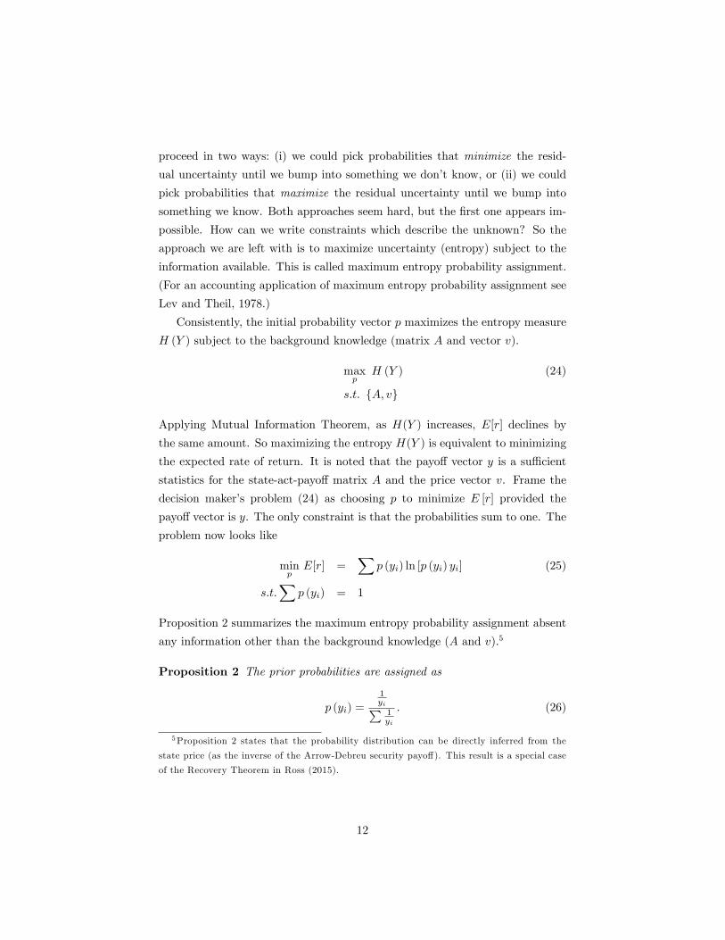
Proposition 2 summarizes the maximum entropy probability assignment absent

any information other than the background knowledge (A and v).5

Proposition 2 The prior probabilities are assigned as

p (yi) =

1yi∑

1yi

. (26)

5Proposition 2 states that the probability distribution can be directly inferred from the

state price (as the inverse of the Arrow-Debreu security payoff). This result is a special case

of the Recovery Theorem in Ross (2015).

12

Proof. Once again the Lagrange multiplier method is fruitful and yields6

p (yi) = λ1

yi. (27)

The probabilities sum to one so that λ is determined as λ = 1/[∑

1yi

]. Plugging

λ in (27) provides (26).

An immediate corollary from Proposition 2 is to determine the expected rate

of return with no information. Substituting the optimal probabilities (26) in the

expected rate of return (25) yields

E [r] =∑ 1

yi∑1yi

ln

(1yi∑

1yi

yi

)

= − ln

(∑ 1

yi

). (28)

Corollary 1 The expected rate of return absent information is the risk free

rate, that is, E [r] = rf .

Proof. Recall yi is the payoff to a scaled Arrow-Debreu security, so 1/yi is the

price of an Arrow-Debreu security with a state payoff of one (previously denoted

si). Hence,∑

1/yi is the price of a risk-free security; that is, one which pays

one unit in all states. The continuously compounded interest rate on the risk-

free investment– the risk free rate rf– can then be derived from the continuous

interest relationship.

1 =

[∑ 1

yi

]erf

⇒ rf = − ln

(∑ 1

yi

)(29)

Comparing (28) and (29) yields E [r] = rf .

Maximum entropy probability assignment implies that the expected rate

of return with no information is the risk free rate– the rate of return from a6Write the Lagrangian function as

L(p;µ) = −∑

p (yi) ln [p (yi) yi]− µ[∑

p (yi)− 1],

where µ is the multiplier. Solving ∂L(·)∂p(yi)

= 0 yields

p (yi) =e−1−µ

yi.

Define λ = e−1−µ as a function of the multiplier µ.

13

security that promises a constant payout. Combining this result with Mutual

Information Theorem provides the right hand side of the central result of this

paper,

E [r|X] = rf + I (X;Y ) . (30)

A Kelly decision maker’s problem can be parameterized such that information

generates an extra return (relative to the risk free rate) exactly equal to the

mutual information– measure of uncertainty reduction.

A numerical example is in order before we proceed to the main result in

section 3.3.

Example 2 Recall from Example 1, the background knowledge is

A =

[1 1

1 4

]and v =

[1

2

]

which can be framed as the vector of payoffs for Arrow-Debreu securities

y =

[3/2

3

].

As a risk free security is already available in A, it is easy to see the risk free

(and no information) rate of return is

rf = − ln

(2

3+

1

3

)= 0.

As 1/yi already sums to one, the maximum entropy state probabilities are p1 =

2/3 and p2 = 1/3.7 An alternative computation of the risk free rate is

E [r] =∑

p (yi) ln p (yi) yi

=2

3ln

(2

3× 3

2

)+

1

3ln

(1

3× 3

)= 0.

Continue with the example to calculate the expected rate of return when addi-

tional information is available. Start with a perfect information system available

where signal xi predicts yi with certainty. The joint probabilities are defined as

7A risk free rate is positive if and only if the sum of the state prices is less than one. Suppose

the state-act-payoffmatrix is A =

[3/4 9/5

1 4

]while keeping all the other parameters intact

in the example. Then the risk free rate is rf ' 29%; and the probabilities are p1 = 4/9 and

p2 = 5/9.

14

follows. (Note that the marginal probabilities for y match up with the no infor-

mation benchmark case.)8

p (x, y) y1 y2

x1 2/3 0

x2 0 1/3

Perfect information means there is no residual uncertainty, that is, H (Y |X) =

0. The expected rate of return with perfect information is H (Y ).

E [r|X] = rf + I (X;Y ) = H (Y )−H (Y |X) = H (Y )

= −(

2

3ln

2

3+

1

3ln

1

3

)= ln 3− 2

3ln 2 ' .6365

Alternatively, a Kelly decision maker can bet all his wealth in the state i after

observing xi (so that bi = 1); and earns the expected rate of return E [r|xi] =

ln yi. The expected rate of return E [r|X] is determined as

E [r|X] = p (x1)E [r|x1] + p (x2)E [r|x2]

=2

3

[ln

3

2

]+

1

3[ln 3] ' .6365.

Finally, consider an imperfect information system as represented by the fol-

lowing joint probabilities.

p (x, y) y1 y2

x1 1/3 0

x2 1/3 1/3

The expected rate of return now is determined as

E [r|X] = I (X;Y ) = H (X) +H (Y )−H (X,Y )

=

[−1

3ln

1

3− 2

3ln

2

3

]+

[−2

3ln

2

3− 1

3ln

1

3

]−[− ln

1

3

]=

[ln 3− 2

3ln 2

]+

[ln 3− 2

3ln 2

]− ln 3

' .1744.

So the imperfect information rate of return is a little over 17%. Alternatively, a

Kelly decision maker can bet all his wealth in the first state after observing x1;8The probability p (x, y) = 0 is used for numerical convenience. It is intended to represent

an event with very small probability p (x, y) = ε so that ε approaches to zero. The limiting

case limε→0

ε ln ε = 0 applies.

15

and earns the expected return E [r|x1] = ln y1. After observing x2, the decision

maker equally splits his wealth between the two states and earns the expected

return E [r|x2] = 12 ln

[12y1

]+ 1

2 ln[

12y2

]. The expected rate of return is then

written as

E [r|X] = p (x1)E [r|x1] + p (x2)E [r|x2]

=1

3ln

3

2+

2

3

{1

2ln

[1

2

(3

2

)]+

1

2ln

[1

2(3)

]}' .1744.

3.3 A fundamental theorem of accounting

In this subsection, the central result of this paper, connecting accounting in-

come and asset values (computed under the economic income method) with

expected rate of return, is established. First, the law of large numbers allows

the combination of (19) and (20).

r (X) = E [r|X]

⇔ ln (1 + rp) = E [r] + I (X;Y ) (31)

Second, applying Corollary 1, the relationship (31) becomes

ln (1 + rp) = rf + I (X;Y ) . (32)

Theorem 2

ln

(1 +

income

assets

)= rf + I (X;Y ) (33)

when economic income accounting is done using the information conditioned

expected rate of return as the continuously compounded accounting discount rate.

Theorem 2 is fundamental in that it equates accounting numbers with infor-

mation numbers. That is, balance sheets and income statements tell how much

information an entity obtains in terms of reduced entropy (without spelling out

what the information is).

Theorem 2 holds as long as (i) the state-act-payoff matrix that describes

a decision problem has full rank in that it can be scaled to an Arrow-Debreu

matrix; (ii) the scaled Arrow-Debreu securities’payoffs are positive as implied

by arbitrage-free pricing and prevent taking logarithm of negative amounts; and

16

(iii) the decision problem is long run in nature so that maximizing the expected

rate of return is equivalent to maximizing terminal wealth and the expected rate

of return is best approximated by the realized rate of return, both are implied

by the law of large numbers.

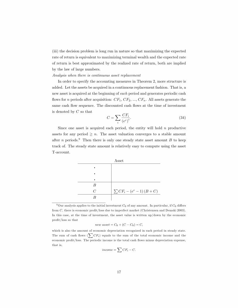
Analysis when there is continuous asset replacement

In order to specify the accounting measures in Theorem 2, more structure is

added. Let the assets be acquired in a continuous replacement fashion. That is, a

new asset is acquired at the beginning of each period and generates periodic cash

flows for n periods after acquisition: CF1, CF2, ..., CFn. All assets generate the

same cash flow sequence. The discounted cash flows at the time of investment

is denoted by C so that

C =∑i

CFi

(er)i. (34)

Since one asset is acquired each period, the entity will hold n productive

assets for any period ≥ n. The asset valuation converges to a stable amount

after n periods.9 Then there is only one steady state asset amount B to keep

track of. The steady state amount is relatively easy to compute using the asset

T-account.

Asset

���B

C∑CFi − (er − 1) (B + C)

B

9Our analysis applies to the initial investment C0 of any amount. In particular, if C0 differs

from C, there is economic profit/loss due to imperfect market (Christensen and Demski 2003).

In this case, at the time of investment, the asset value is written up/down by the economic

profit/loss so that

new asset = C0 + (C − C0) = C,

which is also the amount of economic depreciation recognized in each period in steady state.

The sum of cash flows (∑

CFi) equals to the sum of the total economic income and the

economic profit/loss. The periodic income is the total cash flows minus depreciation expense,

that is,

income =∑

CFi − C.

17

The economic depreciation is∑CFi−(er − 1) (B + C), where (er − 1) (B + C)

is the economic income for the period, and∑CFi while equal to the total cash

inflows over n periods from one asset, is also, conveniently, equal to one period’s

total cash inflows from n assets.10 Every period there is always one asset fully

depreciated so that the total depreciation is equal to the initial cost C:

C =∑

CFi − (er − 1) (B + C)

⇒ Ber −B + Cer =∑

CFi

⇒ B =

∑CFi − erCer − 1

. (35)

The asset value B in steady state is the present value of a perpetuity of the

amount of net cash received in each period (that is,∑CFi less the adjusted cost

erC). The relationship in Theorem 2 can be verified for the case of continuous

asset replacement.

income

assets=

∑CFi − CB + C

=(er − 1) (B + C)

B + C= er − 1

⇒ r = ln

(1 +

income

B + C

)(36)

To construct illuminating (it is hoped) numerical examples, it is necessary to

specify the time sequence of cash flows. A convenient way to do so is a "timing"10Define BVt as the book value at the end of period t. Then the beginning book value for

period 1 is BV0 = 0; and the ending book value for period 1 is BV1 = erC−CF1. The endingbook value for period 2 is BV2 =

(e2r + er

)C − CF2 − (er + 1)CF1. Similarly, the ending

book value for period n is

BVn =

n∑i=1

(er)i C −n∑i=1

CFi

n+1−i∑j=1

(er)j−1

⇒ BVn =

er (1− enr)1− er

C −n∑i=1

CFi

[1− (er)n+1−i

1− er

].

Since C is the discounted cash flow, C =n∑i=1

[CFi/ (e

r)i], it must be (er)n+1 C =

n∑i=1

[CFi (e

r)n+1−i]. Substituting in the expression BVn yields

BVn =er

1− erC − (er)n+1

1− erC −

n∑i=1

CFi

[1

1− er

]+

n∑i=1

CFi

[(er)n+1−i

1− er

]

=er

1− erC −

n∑i=1

CFi

[1

1− er

],

an expression that is independent of n and is also consistent with (35) in the text.

18

vector, k,

k =[k1 k2 � � � kn

](37)

where∑ki = 1. The cash flow for each asset in period i after acquisition is a

function of an optimal information conditioned act, and defined as

CFi = ki (er)i . (38)

With these additional structure, the economic value of the acquired asset is

scaled to one.

C =∑i

ki (er)i

(er)i

= 1 (39)

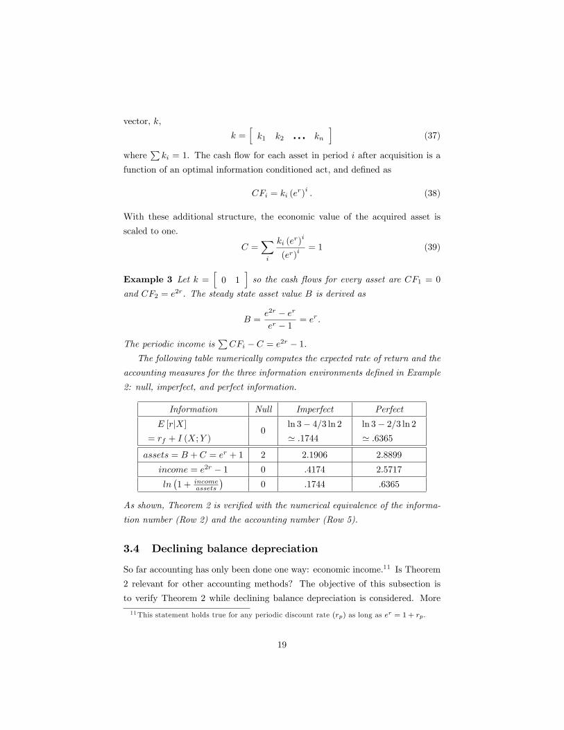
Example 3 Let k =[

0 1]so the cash flows for every asset are CF1 = 0

and CF2 = e2r. The steady state asset value B is derived as

B =e2r − erer − 1

= er.

The periodic income is∑CFi − C = e2r − 1.

The following table numerically computes the expected rate of return and the

accounting measures for the three information environments defined in Example

2: null, imperfect, and perfect information.

Information Null Imperfect Perfect

E [r|X]

= rf + I (X;Y )0

ln 3− 4/3 ln 2

' .1744

ln 3− 2/3 ln 2

' .6365

assets = B + C = er + 1 2 2.1906 2.8899

income = e2r − 1 0 .4174 2.5717

ln(1 + income

assets

)0 .1744 .6365

As shown, Theorem 2 is verified with the numerical equivalence of the informa-

tion number (Row 2) and the accounting number (Row 5).

3.4 Declining balance depreciation

So far accounting has only been done one way: economic income.11 Is Theorem

2 relevant for other accounting methods? The objective of this subsection is

to verify Theorem 2 while declining balance depreciation is considered. More

11This statement holds true for any periodic discount rate (rp) as long as er = 1 + rp.

19

specifically, consider the continuous asset replacement setting in which an asset

with cost C0 is acquired at the beginning of each period.

Let D be the declining rate under declining balance depreciation. The pe-

riodic depreciation is the asset available for production at the beginning of the

period multiplied by the declining rate D. The asset value converges to BD in

steady state.12 The T-account analysis supplies a representation.

Asset

���BD

C0 D(BD + C0

)BD

If under declining balance depreciation, the accounting rate of return (income di-

vided by assets) replicates the discount rate under the economic income method,

then Theorem 2 holds. This requires a well-designed declining rate D.13

12Define BVB as the beginning book value and BVE as the ending book value. At the

beginning of each period, a new asset with cost C0 is purchased. The declining rate is D. The

asset T-account structure can be written as

BVE = (1−D) (BVB + C0) .

The beginning book value for period 1 is BVB = 0 and the ending book value is BVE =

(1−D)C0. The ending book value for period n is

BVE =

(n∑i=1

(1−D)i)C0

=

[1− (1−D)n

D

](1−D)C0.

In the limit, the ending book value converges to a constant.

limn−→∞

BVE =

(1−DD

)C0,

an expression that is independent of n and is also consistent with (44) in the text.13 In general, accounting income seldom coincides with economic income. (Please see

Solomons (1961) and Littleton (2011) on this issue.) We highlight that if the goal is to

convey information numbers through accounting numbers, then an accrual policy must ensure

the equivalence relation holds– that is, the accounting rate of return replicates incomeasset

under

the economic income method.

20

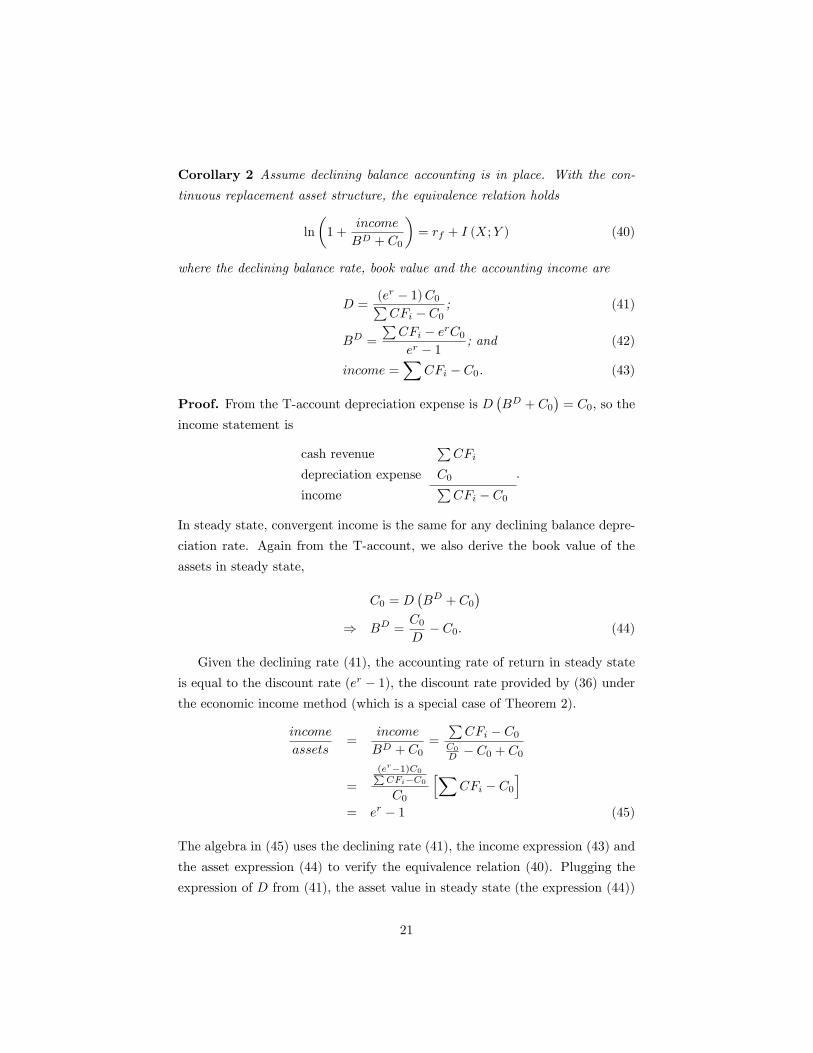
Corollary 2 Assume declining balance accounting is in place. With the con-

tinuous replacement asset structure, the equivalence relation holds

ln

(1 +

income

BD + C0

)= rf + I (X;Y ) (40)

where the declining balance rate, book value and the accounting income are

D =(er − 1)C0∑CFi − C0

; (41)

BD =

∑CFi − erC0

er − 1; and (42)

income =∑

CFi − C0. (43)

Proof. From the T-account depreciation expense is D(BD + C0

)= C0, so the

income statement is

cash revenue∑CFi

depreciation expense C0

income∑CFi − C0

.

In steady state, convergent income is the same for any declining balance depre-

ciation rate. Again from the T-account, we also derive the book value of the

assets in steady state,

C0 = D(BD + C0

)⇒ BD =

C0

D− C0. (44)

Given the declining rate (41), the accounting rate of return in steady state

is equal to the discount rate (er − 1), the discount rate provided by (36) under

the economic income method (which is a special case of Theorem 2).

income

assets=

income

BD + C0=

∑CFi − C0

C0D − C0 + C0

=

(er−1)C0∑CFi−C0C0

[∑CFi − C0

]= er − 1 (45)

The algebra in (45) uses the declining rate (41), the income expression (43) and

the asset expression (44) to verify the equivalence relation (40). Plugging the

expression of D from (41), the asset value in steady state (the expression (44))

21

is derived as

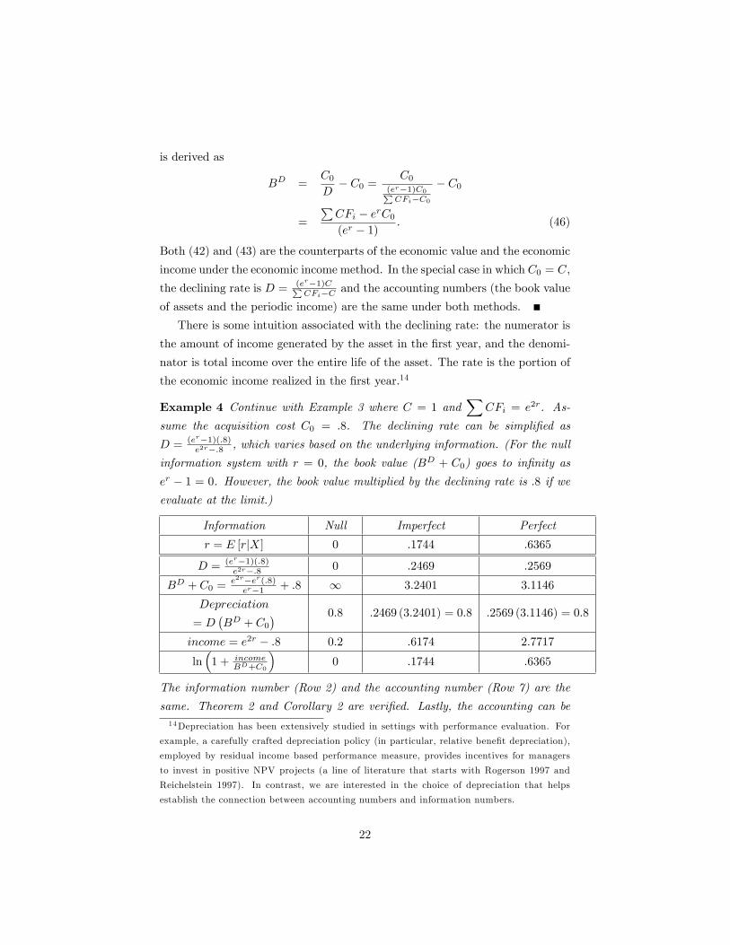
BD =C0

D− C0 =

C0

(er−1)C0∑CFi−C0

− C0

=

∑CFi − erC0

(er − 1). (46)

Both (42) and (43) are the counterparts of the economic value and the economic

income under the economic income method. In the special case in which C0 = C,

the declining rate is D = (er−1)C∑CFi−C and the accounting numbers (the book value

of assets and the periodic income) are the same under both methods.

There is some intuition associated with the declining rate: the numerator is

the amount of income generated by the asset in the first year, and the denomi-

nator is total income over the entire life of the asset. The rate is the portion of

the economic income realized in the first year.14

Example 4 Continue with Example 3 where C = 1 and∑

CFi = e2r. As-

sume the acquisition cost C0 = .8. The declining rate can be simplified as

D = (er−1)(.8)e2r−.8 , which varies based on the underlying information. (For the null

information system with r = 0, the book value (BD + C0) goes to infinity as

er − 1 = 0. However, the book value multiplied by the declining rate is .8 if we

evaluate at the limit.)

Information Null Imperfect Perfect

r = E [r|X] 0 .1744 .6365

D = (er−1)(.8)e2r−.8 0 .2469 .2569

BD + C0 = e2r−er(.8)er−1 + .8 ∞ 3.2401 3.1146

Depreciation

= D(BD + C0

) 0.8 .2469 (3.2401) = 0.8 .2569 (3.1146) = 0.8

income = e2r − .8 0.2 .6174 2.7717

ln(

1 + incomeBD+C0

)0 .1744 .6365

The information number (Row 2) and the accounting number (Row 7) are the

same. Theorem 2 and Corollary 2 are verified. Lastly, the accounting can be14Depreciation has been extensively studied in settings with performance evaluation. For

example, a carefully crafted depreciation policy (in particular, relative benefit depreciation),

employed by residual income based performance measure, provides incentives for managers

to invest in positive NPV projects (a line of literature that starts with Rogerson 1997 and

Reichelstein 1997). In contrast, we are interested in the choice of depreciation that helps

establish the connection between accounting numbers and information numbers.

22

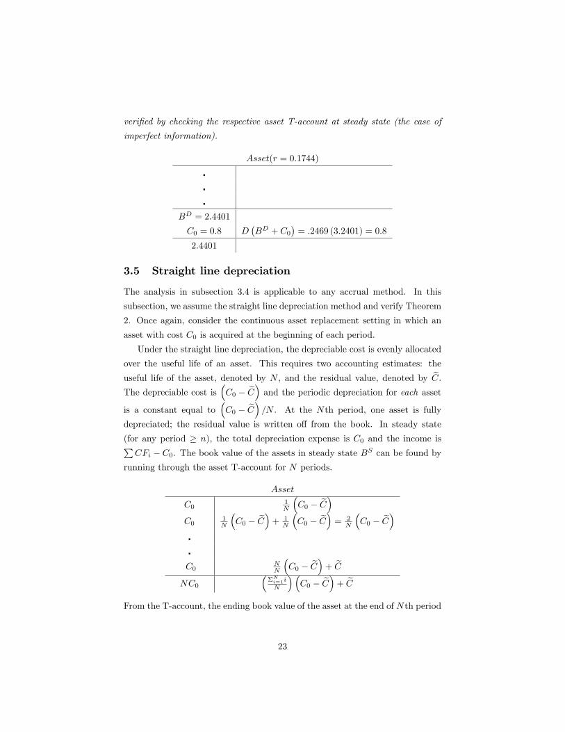
verified by checking the respective asset T-account at steady state (the case of

imperfect information).

Asset(r = 0.1744)

���

BD = 2.4401

C0 = 0.8 D(BD + C0

)= .2469 (3.2401) = 0.8

2.4401

3.5 Straight line depreciation

The analysis in subsection 3.4 is applicable to any accrual method. In this

subsection, we assume the straight line depreciation method and verify Theorem

2. Once again, consider the continuous asset replacement setting in which an

asset with cost C0 is acquired at the beginning of each period.

Under the straight line depreciation, the depreciable cost is evenly allocated

over the useful life of an asset. This requires two accounting estimates: the

useful life of the asset, denoted by N , and the residual value, denoted by C.

The depreciable cost is(C0 − C

)and the periodic depreciation for each asset

is a constant equal to(C0 − C

)/N . At the Nth period, one asset is fully

depreciated; the residual value is written off from the book. In steady state

(for any period ≥ n), the total depreciation expense is C0 and the income is∑CFi − C0. The book value of the assets in steady state BS can be found by

running through the asset T-account for N periods.

Asset

C01N

(C0 − C

)C0

1N

(C0 − C

)+ 1

N

(C0 − C

)= 2

N

(C0 − C

)��C0

NN

(C0 − C

)+ C

NC0

(ΣNi=1iN

)(C0 − C

)+ C

From the T-account, the ending book value of the asset at the end of Nth period

23

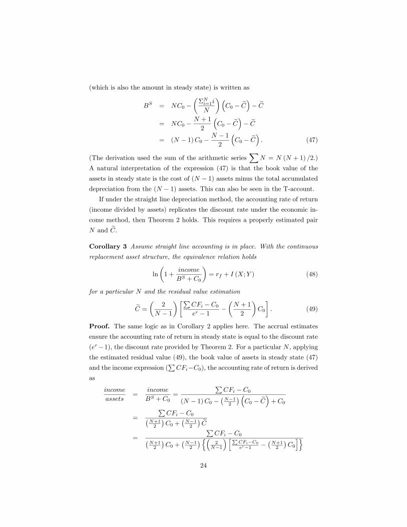
(which is also the amount in steady state) is written as

BS = NC0 −(

ΣNi=1i

N

)(C0 − C

)− C

= NC0 −N + 1

2

(C0 − C

)− C

= (N − 1)C0 −N − 1

2

(C0 − C

). (47)

(The derivation used the sum of the arithmetic series∑

N = N (N + 1) /2.)

A natural interpretation of the expression (47) is that the book value of the

assets in steady state is the cost of (N − 1) assets minus the total accumulated

depreciation from the (N − 1) assets. This can also be seen in the T-account.

If under the straight line depreciation method, the accounting rate of return

(income divided by assets) replicates the discount rate under the economic in-

come method, then Theorem 2 holds. This requires a properly estimated pair

N and C.

Corollary 3 Assume straight line accounting is in place. With the continuous

replacement asset structure, the equivalence relation holds

ln

(1 +

income

BS + C0

)= rf + I (X;Y ) (48)

for a particular N and the residual value estimation

C =

(2

N − 1

)[∑CFi − C0

er − 1−(N + 1

2

)C0

]. (49)

Proof. The same logic as in Corollary 2 applies here. The accrual estimates

ensure the accounting rate of return in steady state is equal to the discount rate

(er−1), the discount rate provided by Theorem 2. For a particular N , applying

the estimated residual value (49), the book value of assets in steady state (47)

and the income expression (∑CFi−C0), the accounting rate of return is derived

as

income

assets=

income

BS + C0=

∑CFi − C0

(N − 1)C0 −(N−1

2

) (C0 − C

)+ C0

=

∑CFi − C0(

N+12

)C0 +

(N−1

2

)C

=

∑CFi − C0(

N+12

)C0 +

(N−1

2

){(2

N−1

) [∑CFi−C0er−1 −

(N+1

2

)C0

]}24

=

∑CFi − C0(

N+12

)C0 +

[∑CFi−C0er−1 −

(N+1

2

)C0

]= er − 1. (50)

The equivalence relation (48) is verified.

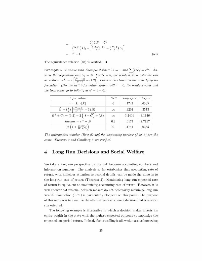
Example 5 Continue with Example 3 where C = 1 and∑

CFi = e2r. As-

sume the acquisition cost C0 = .8. For N = 5, the residual value estimate can

be written as C = 2[e2r−(.8)er−1 − (1.2)

], which varies based on the underlying in-

formation. (For the null information system with r = 0, the residual value and

the book value go to infinity as er − 1 = 0.)

Information Null Imperfect Perfect

r = E [r|X] 0 .1744 .6365

C =(

12

) [ e2r−(.8)er−1 − 3 (.8)

]∞ .4201 .3573

BS + C0 = (3.2)− 2(.8− C

)+ (.8) ∞ 3.2401 3.1146

income = e2r − .8 0.2 .6174 2.7717

ln(

1 + incomeBS+C0

)0 .1744 .6365

The information number (Row 2) and the accounting number (Row 6) are the

same. Theorem 2 and Corollary 3 are verified.

4 Long Run Decisions and Social Welfare

We take a long run perspective on the link between accounting numbers and

information numbers. The analysis so far establishes that accounting rate of

return, with judicious attention to accrual details, can be made the same as to

the long run rate of return (Theorem 2). Maximizing long run expected rate

of return is equivalent to maximizing accounting rate of return. However, it is

well known that rational decision makers do not necessarily maximize long run

wealth. Samuelson (1971) is particularly eloquent on this point. The purpose

of this section is to examine the alternative case where a decision maker is short

run oriented.

The following example is illustrative in which a decision maker invests his

entire wealth in the state with the highest expected outcome to maximize the

expected one period return. Indeed, if short selling is allowed, massive borrowing

25

will occur to finance even larger investments in the preferred outcome, regardless

of the decision maker’s risk preference. This observation stands in contrast

with a Kelly decision maker whose behavior is consistent with long run decision

making. If the decision maker pays attention to accounting numbers, they will

act like long-run decision maker. This induced behavior can be social welfare

beneficial.

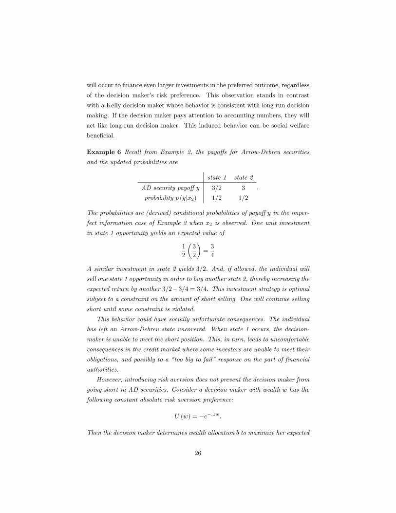
Example 6 Recall from Example 2, the payoffs for Arrow-Debreu securities

and the updated probabilities are

state 1 state 2

AD security payoff y 3/2 3

probability p (y|x2) 1/2 1/2

.

The probabilities are (derived) conditional probabilities of payoff y in the imper-

fect information case of Example 2 when x2 is observed. One unit investment

in state 1 opportunity yields an expected value of

1

2

(3

2

)=

3

4

A similar investment in state 2 yields 3/2. And, if allowed, the individual will

sell one state 1 opportunity in order to buy another state 2, thereby increasing the

expected return by another 3/2−3/4 = 3/4. This investment strategy is optimal

subject to a constraint on the amount of short selling. One will continue selling

short until some constraint is violated.

This behavior could have socially unfortunate consequences. The individual

has left an Arrow-Debreu state uncovered. When state 1 occurs, the decision-

maker is unable to meet the short position. This, in turn, leads to uncomfortable

consequences in the credit market where some investors are unable to meet their

obligations, and possibly to a "too big to fail" response on the part of financial

authorities.

However, introducing risk aversion does not prevent the decision maker from

going short in AD securities. Consider a decision maker with wealth w has the

following constant absolute risk aversion preference:

U (w) = −e−.1w.

Then the decision maker determines wealth allocation b to maximize her expected

26

utility

Maxb

[−1

2e−.1(b1y1) − 1

2e−.1(b2y2)

]s.t. b1 + b2 = 1

and obtains the optimal allocations:

b1 = −.87366

b2 = 1.87366

The risk averse decision maker goes short in state one to the tune of 87% of

initial wealth.

It is important to recall that Kelly "bet your beliefs" behavior will never

go short in an Arrow-Debreu security. As shown in Example 2 (with imperfect

information), a Kelly decision maker, after observing x2, equally splits his wealth

over the two states.

While accounting can not, of course, change preferences, it seems possible

attention paid to accounting numbers could mitigate the tendency to go short

in an Arrow-Debreu security. Non-Kelly behavior necessarily reduces the ac-

counting rate of return calculated in this paper. To the extent that reduced

reported accounting rate of return is a cost decision-makers pay attention to,

a non-Kelly decision maker might act more like a Kelly decision maker. Since

Kelly behavior is socially beneficial, accounting performs a social service.

5 Concluding Remarks

The central result is the equivalence relation between accounting numbers and

an entropy based information metric.

ln

(1 +

income

assets

)= rf + I (X;Y )

There are, perhaps, implications for how to do accounting: it seems plausible

that the accounting numbers of an entity should be supported by its information

capabilities.

But, of course, the equality goes both ways. Just as the information informs

the accounting, it is also the case that accounting can increase our understanding

27

of information. In particular, accounting numbers provides a perfect ranking

of information systems irrespective of the underlying decision context. In this

sense the preceding analysis is in the spirit of Hatfield (1924): Does accounting

deserve a place among other information sciences in this, the information age?

We think the answer is yes.

28

6 References

Akerlof, George, "The market for ‘lemons’: quality uncertainty and the market

mechanism," The Quarterly Journal of Economics 84 (3): 488-500, 1970.

Antle, Rick and John Fellingham, "Capital rationing and organizational

slack in a two-period model," Journal of Accounting Research, 28(1): 1-24,

1990.

Arya, Anil, John Fellingham, and Jonathan Glover, "Teams, repeated tasks

and implicit incentives," Journal of Accounting and Economics, 23: 1997.

Christensen, John A., and Joel Demski, Accounting Theory: An Information

Content Perspective. McGraw-Hill Higher Education, 2003.

Cover, Thomas M., and Joy A. Thomas, Elements of Information Theory.

John Wiley and Sons, 1991.

Demski, Joel, "The general impossibility of normative accounting standard,"

The Accounting Review 48 (4): 718-723, 1973.

Hatfield, Henry, "An historical defense of bookkeeping," Journal of Accoun-

tancy 37 (4): 241-253, 1924.

Jaynes, E. T., Probability Theory: The Logic of Science. Cambridge Univer-

sity Press, 2003.

Kelly, John, "A new interpretation of information rate," Bell Sys. Tech.

Journal, 35: 917-926, 1956.

Lev, Baruch and Henri Theil, "A maximum entropy approach to the choice

of asset depreciation," Journal of Accounting Research, Vol. 16 no. 2: 286-293,

Autumn 1978.

Littleton, A. Charles, "Economists and Accountants," Accounting, Eco-

nomics, and Law : Vol. 1: Iss. 2, Article 2, 2011.

Reichelstein, S, "Investment decisions and managerial performance evalua-

tion," Review of Accounting Studies, 2, 157-180, 1997.

Rogerson, W, "Inter-temporal cost allocation and managerial investment

incentives: a theory explaining the use of economic value added as a performance

measure," Journal of Political Economy, 105, 770-795, 1997.

Ross, Stephen A., Neoclassical Finance. Princeton University Press, 2005.

Ross, Stephen A., "The recovery theorem," The Journal of Finance, Vol.

LXX no. 2: 615-648, 2015.

29

Samuelson, Paul, "Why we should not make mean log of wealth big though

years to act are long," Proceedings National Academy of Science, 68(10), 2493-

2496, 1971.

Shannon, Claude E., "A mathematical theory of communication," Bell Sys.

Tech. Journal, 27: 379-423, 623-656, 1948.

Solomons, David, "Economic and accounting concepts of income," The Ac-

counting Review, 36 (3): 374-383, 1961.

30