a13 eyraud dubois
DESCRIPTION
Here it isTRANSCRIPT

13
Parallel Scheduling of Task Trees with Limited Memory
LIONEL EYRAUD-DUBOIS, INRIA and University of BordeauxLORIS MARCHAL, CNRS and University of LyonOLIVER SINNEN, University of AucklandFREDERIC VIVIEN, INRIA and University of Lyon
This article investigates the execution of tree-shaped task graphs using multiple processors. Each edge ofsuch a tree represents some large data. A task can only be executed if all input and output data fit intomemory, and a data can only be removed from memory after the completion of the task that uses it as aninput data. Such trees arise in the multifrontal method of sparse matrix factorization. The peak memoryneeded for the processing of the entire tree depends on the execution order of the tasks. With one processor,the objective of the tree traversal is to minimize the required memory. This problem was well studied, andoptimal polynomial algorithms were proposed.
Here, we extend the problem by considering multiple processors, which is of obvious interest in theapplication area of matrix factorization. With multiple processors comes the additional objective to minimizethe time needed to traverse the tree—that is, to minimize the makespan. Not surprisingly, this problemproves to be much harder than the sequential one. We study the computational complexity of this problemand provide inapproximability results even for unit weight trees. We design a series of practical heuristicsachieving different trade-offs between the minimization of peak memory usage and makespan. Some ofthese heuristics are able to process a tree while keeping the memory usage under a given memory limit. Thedifferent heuristics are evaluated in an extensive experimental evaluation using realistic trees.
Categories and Subject Descriptors: F.2.0 [Theory of Computation]: Analysis of Algorithms andProblem Complexity—General; F.2.3 [Theory of Computation]: Analysis of Algorithms and ProblemComplexity—Tradeoffs between Complexity Measures; C.1.4 [Computer Systems Organization]: Proces-sor Architectures—Parallel Architectures
General Terms: Algorithms, Performance
Additional Key Words and Phrases: Approximation algorithms, memory usage, multicriteria optimization,pebble game, scheduling, task graphs
ACM Reference Format:Lionel Eyraud-Dubois, Loris Marchal, Oliver Sinnen, and Frederic Vivien. 2015. Parallel scheduling of tasktrees with limited memory. ACM Trans. Parallel Comput. 2, 2, Article 13 (June 2015), 37 pages.DOI: http://dx.doi.org/10.1145/2779052
1. INTRODUCTION
Parallel workloads are often modeled as task graphs, where nodes represent tasks andedges represent the dependencies between tasks. There is an abundant literature ontask graph scheduling when the objective is to minimize the total completion time, or
Authors’ addresses: L. Eyraud-Dubois, INRIA, 200 avenue de la Vieille Tour, 33400 Talence, France;email: [email protected]; L. Marchal and F. Vivien, LIP, ENS-Lyon, 46 allee d’Italie, 69007Lyon, France; emails: [email protected], [email protected]; O. Sinnen, Department of Electri-cal and Computer Engineering, University of Auckland, Private Bag 92019, Auckland, New Zealand; email:[email protected] to make digital or hard copies of part or all of this work for personal or classroom use is grantedwithout fee provided that copies are not made or distributed for profit or commercial advantage and thatcopies show this notice on the first page or initial screen of a display along with the full citation. Copyrights forcomponents of this work owned by others than ACM must be honored. Abstracting with credit is permitted.To copy otherwise, to republish, to post on servers, to redistribute to lists, or to use any component of thiswork in other works requires prior specific permission and/or a fee. Permissions may be requested fromPublications Dept., ACM, Inc., 2 Penn Plaza, Suite 701, New York, NY 10121-0701 USA, fax +1 (212)869-0481, or [email protected]© 2015 ACM 2329-4949/2015/06-ART13 $15.00DOI: http://dx.doi.org/10.1145/2779052
ACM Transactions on Parallel Computing, Vol. 2, No. 2, Article 13, Publication date: June 2015.
13:2 L. Eyraud-Dubois et al.
makespan. However, with the increase of the size of the data to be processed, the mem-ory footprint of the application can have a dramatic impact on the algorithm executiontime and thus needs to be optimized. This is best exemplified with an application that,depending on the way it is scheduled, will either fit in the memory or require the use ofswap mechanisms or out-of-core techniques. There are very few existing studies on theminimization of the memory footprint when scheduling task graphs, and even fewer ofthem targeting parallel systems.
We consider the following memory-aware parallel scheduling problem for rootedtrees. The nodes of the tree correspond to tasks, and the edges correspond to thedependencies among the tasks. The dependencies are in the form of input and outputfiles1: each node takes as input several large files, one for each of its children, and itproduces a single large file; the different files may have different sizes. Furthermore,the execution of any node requires its execution file to be present; the execution filemodels the program and/or the temporary data of the task. We are to execute such a setof tasks on a parallel system made of p identical processing resources sharing the samememory. The execution scheme corresponds to a schedule of the tree where processinga node of the tree translates into reading the associated input files and producing theoutput file. How can the tree be scheduled to optimize the memory usage?
Modern computing platforms exhibit a complex memory hierarchy ranging fromcaches to RAM and disks and even sometimes tape storage, with the classical propertythat the smaller the memory, the faster. Thus, to avoid large running times, one usuallywants to avoid the use of memory devices whose IO bandwidth is below a given thresh-old: even if out-of-core execution (when large data are unloaded to disks) is possible, thisrequires special care when programming the application and one usually wants to stayin the main memory (RAM). This is why, in this article, we are interested in the questionof minimizing the amount of main memory needed to completely process an application.
Throughout the article, we consider in-trees, where a task can be executed only if allof its children have already been executed (This is absolutely equivalent to consideringout-trees as a solution, as an in-tree can be transformed into a solution for the corre-sponding out-tree by just reversing the direction of time, as outlined in Jacquelin et al.[2011]). A task can be processed only if all of its files (input, output, and execution) fit incurrently available memory. At a given time, many files may be stored in the memory,and at most p tasks may be processed by the p processors. This is obviously possibleonly if all tasks and execution files fit in memory. When a task finishes, the memoryneeded for its execution file and its input files is released. Clearly, the schedule thatdetermines the processing times of each task plays a key role in determining whichamount of main memory is needed for a successful execution of the entire tree.
The motivation for this work comes from numerical linear algebra, and especiallythe factorization of sparse matrices using direct multifrontal methods [Davis 2006].During the factorization, the computations are organized as a tree workflow calledthe elimination tree, and the huge size of the data involved makes it absolutely nec-essary to reduce the memory requirement of the factorization. The sequential versionof this problem (i.e., with p = 1 processor) has already been studied. Liu [1986] dis-cusses how to find a memory-minimizing traversal when the traversal is required tocorrespond to a postorder traversal of the tree. A follow-up study [Liu 1987] presentsan optimal algorithm to solve the general problem, without the postorder constrainton the traversal. Postorder traversals are known to be arbitrarily worse than opti-mal traversals for memory minimization [Jacquelin et al. 2011]. However, they arevery natural and straightforward solutions to this problem, as they allow the full
1The concept of file is used here in a very general meaning and does not necessarily correspond to a classicalfile on a disk. Essentially, a file is a set of data.
ACM Transactions on Parallel Computing, Vol. 2, No. 2, Article 13, Publication date: June 2015.

Parallel Scheduling of Task Trees with Limited Memory 13:3
processing of one subtree before starting a new one. Therefore, they are widely usedin sparse matrix software like MUMPS [Amestoy et al. 2001, 2006], and in practice, theyachieve close to optimal performance on actual elimination trees [Jacquelin et al. 2011].Note that we consider here that no numerical pivoting is performed during the factor-ization and thus that all characteristics of the task tree (length of tasks, size of thedata) are known before the computation really happens. Moreover, even if some soft-ware (including MUMPS) are able to distribute the processing of each task to multipleprocessors, here we focus on the case where each task has to be processed by a singleprocessor, and we keep the extension to parallel tasks for future work.
The parallel version of this problem is a natural continuation of these studies: whenprocessing large elimination trees, we would like to take advantage of parallel pro-cessing resources. However, to the best of our knowledge, no theoretical study existsfor this problem. A preliminary version of this work, with fewer complexity resultsand proposed heuristics, was presented at IPDPS 2013 [Marchal et al. 2013]. The keycontributions of this work are as follows:
—A new proof that the parallel variant of the pebble-game problem is NP-complete(simpler than in Marchal et al. [2013]). This shows that the introduction of mem-ory constraints, in the simplest cases, suffices to make the problem NP-hard(Theorem 4.2).
—The proof that no schedule can simultaneously achieve a constant-ratio approxima-tion for the memory minimization and for the makespan minimization (Theorem 4.4);bounds on the achievable approximation ratios for makespan and memory when thenumber of processors is fixed (Theorems 4.5 and 4.6).
—A series of practical heuristics achieving different trade-offs between the minimiza-tion of peak memory usage and makespan; some of these heuristics are guaranteedto keep the memory under a given memory limit.
—An exhaustive set of simulations using realistic tree-shaped task graphs correspond-ing to elimination trees of actual matrices; the simulations assess the relative andabsolute performance of the heuristics.
The rest of this article is organized as follows. Section 2 reviews related studies.The notation and formalization of the problem are introduced in Section 3. Complexityresults are presented in Section 4, whereas Section 5 proposes different heuristics tosolve the problem, which are evaluated in Section 6.
2. BACKGROUND AND RELATED WORK
2.1. Sparse Matrix Factorization
As mentioned earlier, determining a memory-efficient tree traversal is very importantin sparse numerical linear algebra. The elimination tree is a graph-theoretical modelthat represents the storage requirements, and computational dependencies and re-quirements, in the Cholesky and LU factorization of sparse matrices. In a previousstudy [Jacquelin et al. 2011], we described how such trees are built and how the multi-frontal method [Liu 1992] organizes the computations along the tree. This is the contextof the founding studies of Liu [1986, 1987] on memory minimization for postorder orgeneral tree traversals presented in the previous section. Memory minimization is stilla concern in modern multifrontal solvers when dealing with large matrices. Effortshave been made to design dynamic schedulers that take into account dynamic pivoting(which impacts the weights of edges and nodes) when scheduling elimination treeswith strong memory constraints [Guermouche and L’Excellent 2004], or to considerboth task and tree parallelism with memory constraints [Agullo et al. 2012]. Althoughthese studies try to optimize memory management in existing parallel solvers, we aimat designing a simple model to study the fundamental underlying scheduling problem.
ACM Transactions on Parallel Computing, Vol. 2, No. 2, Article 13, Publication date: June 2015.

13:4 L. Eyraud-Dubois et al.
2.2. Scientific Workflows
The problem of scheduling a task graph under memory constraints also appears inthe processing of scientific workflows whose tasks require large I/O files. Such work-flows arise in many scientific fields, such as image processing, genomics, or geophysicalsimulations. The problem of task graphs handling large data has been identified inRamakrishnan et al. [2007], which proposes some simple heuristic solutions. Surpris-ingly, in the context of quantum chemistry computations, Lam et al. [2011] have re-cently rediscovered the algorithm published in 1987 in Liu [1987].
2.3. Pebble Game and Its Variants
On the more theoretical side, this work builds on the many papers that have addressedthe pebble game and its variants. The pioneering work of Sethi and Ullman [1970] onregister allocation has been formalized as a pebble game on directed graphs in Gilbertet al. [1980] with the following rules:
(i) A pebble may be removed from a vertex at any time.(ii) A pebble may be placed on a source node at any time.
(iii) If all predecessors of an unpebbled vertex v are pebbled, a pebble may be placedon v.
In Sethi and Ullman [1970], the authors seek to minimize the number of registers thatare needed to compute an arithmetic expression, which is naturally described as a tree.In this context, pebbling a node corresponds to loading an input (rule (ii)) or computinga particular subexpression (rule (iii)). They show how to compute, in polynomial time,a pebbling scheme that uses a minimum number of pebbles for in-trees. The problem ofdetermining whether a general DAG can be executed with a given number of pebbleshas been shown NP-hard by Sethi [1973] if no vertex is pebbled more than once. Thegeneral problem allowing recomputation—that is, repebbling a vertex that has beenpebbled before—has been proven PSPACE complete [Gilbert et al. 1980].
The pebble-game problem translates into a simple instance of our problem when allI/O files have size 1 and all execution files have size 0. To the best of our knowledge,there have been no attempts to extend these results to parallel machines, with theobjective of minimizing both memory and total execution time. We present such anextension in Section 4.
3. MODEL AND OBJECTIVES
3.1. Application Model
In this paper, we consider a tree-shaped task graph T composed of n nodes, or tasks,numbered from 1 to n. Nodes in the tree have an output file, an execution file (orprogram), and several input files (one per child). More precisely,
—Each node i in the tree has an execution file of size ni, and its processing on aprocessor takes time wi.
—Each node i has an output file of size fi. If i is not the root, its output file is usedas input by its parent parent(i); if i is the root, its output file can be of size zero orcontain outputs to the outside world.
—Each non–leaf node i in the tree has one input file per child. We denote by Children(i)the set of the children of i. For each child j ∈ Children(i), task j produces a file ofsize f j for i. If i is a leaf node, then Children(i) = ∅ and i has no input file: we assumethat the initial data of the task either resides in its execution file or is read from disk(or received from the outside word) during the execution of the task.
ACM Transactions on Parallel Computing, Vol. 2, No. 2, Article 13, Publication date: June 2015.

Parallel Scheduling of Task Trees with Limited Memory 13:5
During the processing of a task i, the memory must contain its input files, theexecution file, and the output file. The memory needed for this processing is thus⎛
⎝ ∑j∈Children(i)
f j
⎞⎠ + ni + fi.
After i has been processed, its input files and execution file (program) are discarded,whereas its output file is kept in memory until the processing of its parent.
3.2. Platform Model and Objectives
In this work, our goal is to design a simple platform model that allows the study ofmemory minimization on a parallel platform. We thus consider p identical processorssharing a single memory.
Any sequential optimal schedule for memory minimization is obviously an opti-mal schedule for memory minimization on a platform with any number p of proces-sors. Therefore, memory minimization on parallel platforms is only meaningful in thescope of multicriteria approaches that consider trade-offs between the following twoobjectives:
—Makespan: The classical makespan, or total execution time, which corresponds to thetime span between the beginning of the execution of the first leaf task and the endof the processing of the root task.
—Memory: The amount of memory needed for the computation. At each timestep,some files are stored in the memory and some task computations occur, inducing amemory usage. The peak memory is the maximum usage of the memory over thewhole schedule, hence the memory that needs to be available, which we aim tominimize.
4. COMPLEXITY RESULTS IN THE PEBBLE-GAME MODEL
Since there are two objectives, the decision version of our problem can be stated asfollows.
Definition 4.1 (BiObjectiveParallelTreeScheduling). Given a tree-shaped task graphT with file sizes and task execution times, p processors, and two bounds BCmax andBmem, is there a schedule of the task graph on the processors whose makespan is notlarger than BCmax and whose peak memory is not larger than Bmem?
This problem is obviously NP-complete. Indeed, when there are no memory con-straints (Bmem = ∞) and when the task tree does not contain any inner node—that is,when all tasks are either leaves or the root—then our problem is equivalent to schedul-ing independent tasks on a parallel platform that is an NP-complete problem as soonas tasks have different execution times [Lenstra et al. 1977]. Conversely, minimizingthe makespan for a tree of same-size tasks can be solved in polynomial time when thereare no memory constraints [Hu 1961]. In this section, we consider the simplest variantof the problem. We assume that all input files have the same size (∀i, fi = 1) and noextra memory is needed for computation (∀i, ni = 0). Furthermore, we assume that theprocessing of each node takes unit time: ∀i, wi = 1. We call this variant of the problemthe pebble-game model because it perfectly corresponds to the pebble-game problemsintroduced earlier: the weight fi = 1 corresponds to the pebble that one must put onnode i to process it; this pebble must remain there until the parent of node i has beencompleted, as the parent of node i uses as input the output of node i. Processing a nodeis done in unit time.
ACM Transactions on Parallel Computing, Vol. 2, No. 2, Article 13, Publication date: June 2015.

13:6 L. Eyraud-Dubois et al.
Fig. 1. Tree used for the NP-completeness proof.
In this section, we first show that, even in this simple variant, the introductionof memory constraints (a limit on the number of pebbles) makes the problem NP-hard (Section 4.1). Then, we show that when trying to minimize both memory andmakespan, it is not possible to get a solution with a constant approximation ratio forboth objectives, and we provide tighter ratios when the number of processors is fixed(Section 4.2).
4.1. NP-Completeness
THEOREM 4.2. The BiObjectiveParallelTreeScheduling problem is NP-complete in thepebble-game model (i.e., with ∀i, fi = wi = 1, ni = 0).
PROOF. First, it is straightforward to check that the problem is in NP: given aschedule, it is easy to compute its peak memory and makespan.
To prove the problem NP-hard, we perform a reduction from 3-PARTITION, which isknown to be NP-complete in the strong sense [Garey and Johnson 1979]. We considerthe following instance I1 of the 3-PARTITION problem: let ai be 3m integers and B aninteger such that
∑ai = mB. We consider the variant of the problem, also NP-complete,
where ∀i, B/4 < ai < B/2. To solve I1, we need to solve the following question: doesthere exist a partition of the ai ’s in m subsets S1, . . . , Sm, each containing exactly threeelements, such that for each Sk,
∑i∈Sk
ai = B? We build the following instance I2
of our problem, illustrated in Figure 1. The tree contains a root r with 3m children,the Ni ’s, each one corresponding to a value ai. Each node Ni has 3m × ai children,Li
1, . . . , Li3m×ai
, which are leaf nodes. The question is to find a schedule of this tree onp = 3mB processors, whose peak memory is not larger than Bmem = 3mB + 3m andwhose makespan is not larger than BCmax = 2m+ 1.
Assume first that there exists a solution to I1—in other words, that there are msubsets Sk of three elements with
∑i∈Sk
ai = B. In this case, we build the followingschedule:
—At step 1, we process all of the nodes Li1x , Lj1
y , and Lk1z with S1 = {ai1 , aj1 , ak1}. There
are 3mB = p such nodes, and the amount of memory needed is also 3mB.—At step 2, we process the nodes Ni1 , Nj1 , Nk1 . The memory needed is 3mB+ 3.—At step 2n + 1, with 1 ≤ n ≤ m− 1, we process the 3mB = p nodes Lin
x , Ljny , Lkn
z withSn = {ain, ajn, akn}. The amount of memory needed is 3mB+ 3n (counting the memoryfor the output files of the Nt nodes previously processed).
—At step 2n + 2, with 1 ≤ n ≤ m− 1, we process the nodes Nin, Njn, Nkn. The memoryneeded for this step is 3mB+ 3(n + 1).
—At step 2m+ 1, we process the root node and the memory needed is 3m+ 1.
Thus, the peak memory of this schedule is Bmem and its makespan BCmax .Reciprocally, assume that there exists a solution to problem I2—that is, there exists a
schedule of makespan at most BCmax = 2m+1. Without loss of generality, we assume thatthe makespan is exactly 2m+1. We start by proving that at any step of the algorithm, at
ACM Transactions on Parallel Computing, Vol. 2, No. 2, Article 13, Publication date: June 2015.

Parallel Scheduling of Task Trees with Limited Memory 13:7
most three of the Ni nodes are being processed. By contradiction, assume that four (ormore) such nodes Nis , Njs , Nks , Nls are processed during a certain step s. We recall thatai > B/4 so that ais + ajs + aks + als > B and thus ais + ajs + aks + als ≥ B+ 1. The memoryneeded at this step is thus at least (B+ 1)3m for the children of the nodes Nis , Njs , Nks ,and Nls and 4 for the nodes themselves, hence a total of at least (B+ 1)3m+ 4, which ismore than the prescribed bound Bmem. Thus, at most three Ni nodes are processed at anystep. In the considered schedule, the root node is processed at step 2m+1. Then, at step2m, some of the Ni nodes are processed, and at most three of them from what precedes.The ai ’s corresponding to those nodes make the first subset S1. Then, all nodes Lj
x suchthat aj ∈ S1 must have been processed at the latest at step 2m− 1, and they occupy amemory footprint of 3m
∑aj∈S1
aj at steps 2m−1 and 2m. Let us assume that a node Nk isprocessed at step 2m−1. For the memory bound Bmem to be satisfied, we must have ak+∑
aj∈S1aj ≤ B. (Otherwise, we would need a memory of at least 3m(B+1) for the involved
Ljx nodes plus 1 for the node Nk). Therefore, node Nk can as well be processed at step
2m instead of step 2m− 1. We then modify the schedule to schedule Nk at step 2m andthus add k to S1. We can therefore assume, without loss of generality, that no Ni node isprocessed at step 2m−1. Then, at step 2m−1, only the children of the Nj nodes with aj ∈S1 are processed, and all of them are. So, none of them have any memory footprint beforestep 2m−1. We then generalize this analysis: at step 2i, for 1 ≤ i ≤ m−1, only some Njnodes are processed and they define a subset Si; at step 2i−1, for 1 ≤ i ≤ m−1, the onlyprocessed nodes are the nodes Lk
x that are children of the nodes Nj such that aj ∈ Si.Because of the memory constraint, each of the m subsets of ai ’s built earlier sum to
at most B. Since they contain all ai ’s, their sum is mB. Thus, each subset Sk sums to B,and we have built a solution for I1.
4.2. Joint Minimization of Both Objectives
As our problem is NP-complete, it is natural to wonder whether approximation algo-rithms can be designed. In this section, we prove that there does not exist any schedul-ing algorithm that approximates both the minimum makespan and the minimum peakmemory with constant factors. This is equivalent to saying that there is no Zenith (alsocalled simultaneous) approximation. We first state a lemma, valid for any tree-shapedtask graph, which provides lower bounds for the makespan of any schedule.
LEMMA 4.3. For any schedule S on p processors with a peak memory M, we have thetwo following lower bounds on the makespan Cmax:
Cmax ≥ 1p
n∑i=1
wi
M × Cmax ≥n∑
i=1
⎛⎝ni + fi +
∑j∈Children(i)
f j
⎞⎠ wi.
In the pebble-game model, these equations can be written as
Cmax ≥ n/pM × Cmax ≥ 2n − 1.
PROOF. The first inequality is a classical bound stating that all tasks must be pro-cessed before Cmax.
Similarly, each task i uses a memory of ni+fi+∑
j∈Children(i) f j during a time wi. Hence,the total memory usage (i.e., the sum over all time instants t of the memory used by
ACM Transactions on Parallel Computing, Vol. 2, No. 2, Article 13, Publication date: June 2015.

13:8 L. Eyraud-Dubois et al.
Fig. 2. Tree used for establishing Theorem 4.4.
S at time t) needs to be at least equal to∑n
i=1(ni + fi + ∑j∈Children(i) f j)wi. Because S
uses a memory that is not larger than M at any time, the total memory usage is upperbounded by M × Cmax. This gives us the second inequality. In the pebble-game model,the right-hand term of the second inequality can be simplified:
n∑i=1
⎛⎝ni + fi +
∑j∈Children(i)
f j
⎞⎠ wi =
(n∑
i=1
fi
)+
⎛⎝ n∑
i=1
∑j∈Children(i)
f j
⎞⎠ = n + (n − 1).
In the next theorem, we show that it is not possible to design an algorithm withconstant approximation ratios for both makespan and maximum memory (i.e., approx-imation ratios independent of the number of processors p). In Theorem 4.5, we willprovide a refined version that analyzes the dependence on p.
THEOREM 4.4. For any given constants α and β, there does not exist any algorithmfor the pebble-game model that is both an α-approximation for makespan minimizationand a β-approximation for peak memory minimization when scheduling in-tree taskgraphs.
PROOF. In this proof, we consider the tree depicted in Figure 2. The root of thistree has m children a1, . . . , am. Any of these children, ai, has m children bi,1, . . . , bi,m.Therefore, overall, this tree contains n = 1 + m + m × m nodes. On the one hand,with a large number of processors (namely, m2), this tree can be processed in C∗
max = 3timesteps: all of the leaves are processed in the first step, all of the ai nodes in the secondstep, and finally the root in the third and last step. On the other hand, the minimummemory required to process the tree is M∗ = 2m. This is achieved by processing thetree with a single processor. The subtrees rooted at the ai ’s are processed one at a time.The processing of the subtree rooted at node ai requires a memory of m + 1 (for theprocessing of its root ai once the m leaves have been processed). Once such a subtree isprocessed, there is a unit file that remains in memory. Hence, the peak memory usagewhen processing the j-th of these subtrees is ( j −1)+ (m+1) = j +m. The overall peakM∗ = 2m is thus reached when processing the root of the last of these subtrees.
Let us assume that there exists a schedule S that is both an α-approximation for themakespan and a β-approximation for the peak memory. Then, for the tree of Figure 2,the makespan Cmax of S is at most equal to 3α, and its peak memory M is at mostequal to 2βm. Because n = 1 + m + m2, Lemma 4.3 implies that M × Cmax ≥ 2n− 1 =2m2 + 2m + 1. Therefore, M ≥ 2m2+2m+1
3α. For a sufficiently large value of m, this is
larger than 2βm, the upper bound on M. This contradicts the hypothesis that S is aβ-approximation for peak memory usage.
ACM Transactions on Parallel Computing, Vol. 2, No. 2, Article 13, Publication date: June 2015.

Parallel Scheduling of Task Trees with Limited Memory 13:9
Fig. 3. Tree used to establish Theorem 4.5 for p = 13 processors.
Theorem 4.4 only considers approximation algorithms whose approximation ratiosare constant. In the next theorem we consider algorithms whose approximations ratiosmay depend on the number of processors in the platform.
THEOREM 4.5. When scheduling in-tree task graphs in the pebble-game model on aplatform with p ≥ 2 processors, there does not exist any algorithm that is both an α(p)-approximation for makespan minimization and a β(p)-approximation for peak memoryminimization, with
α(p)β(p) <2p
log(p) + 2·
PROOF. We establish this result by contradiction. We assume that there existsan algorithm that is an α(p)-approximation for makespan minimization and a β(p)-approximation for peak memory minimization when scheduling in-tree task graphs,with α(p)β(p) = 2p
(log(p)+2) − ε with ε > 0.The proof relies on a tree similar to the one depicted in Figure 3 for the case p = 13.
The top part of the tree is a complete binary subtree with p2 leaves, l1, . . . , l p
2 , and ofheight m. Therefore, this subtree contains 2 p
2 − 1 nodes, all of its leaves are at deptheither m or m − 1, and m = 1 + log( p
2 ) = log(p). To prove the last equality, weconsider whether p is even:
—p is even: ∃l ∈ N, p = 2l. Then, 1 + log( p2 ) = log(2 2l
2 ) = log(2l) = log(p).—p is odd: ∃l ∈ N, p = 2l +1. Then, 1+log( p
2 ) = log(2 2l+12 ) = log(2l +2). Since
2l + 1 is odd, log(2l + 2) = log(2l + 1) = log(p).
Each node li is the root of a comb subtree2 of height k (except the last node if p is odd),and each comb subtree contains 2k − 1 nodes. If p is odd, the last leaf of the binarytop subtree, l p
2 , is the root of a chain subtree with k − 1 nodes. Then, the entire treecontains n = pk−1 nodes (be careful not to count the roots of the comb subtrees twice):
2A comb tree is recursively defined either as a single node or a tree whose root has two children: one is a leafand the other is the root of a comb tree.
ACM Transactions on Parallel Computing, Vol. 2, No. 2, Article 13, Publication date: June 2015.

13:10 L. Eyraud-Dubois et al.
—p is even: ∃l ∈ N, p = 2l. Then,
n =(2
⌈ p2
⌉− 1
)+
(⌈ p2
⌉(2k − 2)
)= (2l − 1) + l(2k − 2) = pk − 1.
—p is odd: ∃l ∈ N, p = 2l + 1. Then,
n =(2
⌈ p2
⌉− 1
)+
((⌈ p2
⌉− 1
)(2k − 2)
)+ (k − 2)
= (2(l + 1) − 1) + (l + 1 − 1)(2k − 2) + (k − 2) = (2l + 1)k − 1 = pk − 1.
With the p processors, it is possible to process all comb subtrees (and the chainsubtree if p is odd) in parallel in k steps by using two processors per comb subtree (andone for the chain subtree). Then, m − 1 steps are needed to complete the processingof the binary reduction (the li nodes have already been processed at the last step ofthe processing of the comb subtrees). Thus, the optimal makespan with p processors isC∗
max = k + m− 1.We now compute the optimal peak memory usage, which is obtained with a sequential
processing. Each comb subtree can be processed with three units of memory, if we followany postorder traversal starting from the deepest leaves. We consider the sequentialprocessing of the entire tree that follows a postorder traversal that processes each combsubtree as described previously, that processes first the left-most comb subtree, thenthe second left-most comb subtree, the parent node of these subtrees, and so on, andfinishes with the right-most comb subtree (or the chain subtree if p is odd). The peakmemory is reached when processing the last comb subtree. At that time, either m− 2or m− 1 edges of the binary subtree are stored in memory (depending on the value of p
2 ). The processing of the last comb subtree itself uses three units of memory. Hence,the optimal peak memory is not greater than m+ 2: M∗ ≤ m+ 2.
Let Cmax denote the makespan achieved by the studied algorithm on the tree, andlet M denote its peak memory usage. By definition, the studied algorithm is an α(p)-approximation for the makespan: Cmax ≤ α(p)C∗
max. Thanks to Lemma 4.3, we knowthat
M × Cmax ≥ 2n − 1 = 2pk − 3.
Therefore,
M ≥ 2pk − 3Cmax
≥ 2pk − 3α(p)(k + m− 1)
.
The approximation ratio of the studied algorithm with respect to the peak memoryusage is thus bounded by
β(p) ≥ MM∗ ≥ 2pk − 3
α(p)(k + m− 1)(m+ 2)·
Therefore, if we recall that m = log(p),
α(p)β(p) ≥ 2pk − 3(k + m− 1)(m+ 2)
= 2pk − 3(k + log(p) − 1)(log(p) + 2)
−−−→k→∞
2plog(p) + 2
·
Hence, there exists a value k0 such that for any k ≥ k0,
α(p)β(p) ≥ 2plog(p) + 2
− ε
2·
This contradicts the definition of ε and hence concludes the proof.
Readers may wonder whether the bound in Theorem 4.5 is tight. This question isespecially relevant because the proof of Theorem 4.5 uses the average memory usage
ACM Transactions on Parallel Computing, Vol. 2, No. 2, Article 13, Publication date: June 2015.

Parallel Scheduling of Task Trees with Limited Memory 13:11
Fig. 4. Tree used for establishing Theorem 4.6.
as a lower bound to the peak memory usage. This technique enables one to designa simple proof, which may however be very crude. In fact, in the special case whereα(p) = 1—that is, for makespan-optimal algorithms—a stronger result holds. For thatcase, Theorem 4.5 states that β(p) ≥ 2p
log(p)+2 . Theorem 4.6 states that β(p) ≥ p − 1(which is a stronger bound when p ≥ 4). This result is established through a careful,painstaking analysis of a particular task graph. Using the average memory usageargument on this task graph would not enable one to obtain a nontrivial bound.
THEOREM 4.6. There does not exist any algorithm for the pebble-game model thatis both optimal for makespan minimization and that is a (p − 1 − ε)-approximationalgorithm for the peak memory minimization, where p is the number of processors andε > 0.
PROOF. To establish this result, we proceed by contradiction. Let p be the numberof processors. We then assume that there exists an algorithm A that is optimal formakespan minimization and is a β(p)-approximation for peak memory minimization,with β(p) < p − 1. Thus, there exists ε > 0 such that β(p) = p − 1 − ε.
We start by presenting the tree used to establish this theorem. Then, we computeits optimal peak memory and its optimal makespan. Finally, we derive a lower boundon the memory usage of any makespan-optimal algorithm to obtain the desiredcontradiction.
The tree. Figure 4 presents the tree used to derive a contradiction. This tree is madeof p − 1 identical subtrees whose roots are the children of the tree root. The value of δwill be fixed later on.
Optimal peak memory. A memory-optimal sequential schedule processes each sub-tree rooted at cpi
1 sequentially. Each of these subtrees can be processed with a memoryof δ + 1 by processing first the subtree rooted at di
1, then the one rooted at di2, and so
forth, until the one rooted at diδ−1, and then the chain of ci
j nodes, and the remainingcpi
j nodes. The peak memory, reached when processing the last subtree rooted at cpi1,
is thus δ + p − 1.
Optimal execution time. The optimal execution time with p processors is at leastequal to the length of the critical path. The critical path has a length of δ + k, which is
ACM Transactions on Parallel Computing, Vol. 2, No. 2, Article 13, Publication date: June 2015.

13:12 L. Eyraud-Dubois et al.
the length of the path from the root to any cik node, with 1 ≤ i ≤ p− 1. We now define k
for this lower bound to be an achievable makespan, with an overall schedule as follows:
—Each of the first p − 1 processors processes one of the critical paths from end to end(except obviously for the root node that will only be processed by one of them).
—The last processor processes all of the other nodes. We define k so that this processorfinishes processing all of the nodes it is allocated at time k + δ − 2. This allows theother processors to process all p − 1 nodes cp1
1 through cpp−11 from time k + δ − 2 to
time k + δ − 1.
To find such a value for k, we need to compute the number of nodes allocated to thelast processor. In the subtree rooted in cpi
1, the last processor is in charge of processingthe δ − 1 nodes di
1 through diδ−1, and the descendants of the di
j nodes, for 1 ≤ j ≤ δ − 1.As node di
j has δ − j + 1 descendants, the number of nodes in the subtree rooted in cpi1
that are allocated to the last processor is equal to
(δ − 1) +δ−1∑j=1
(δ − j + 1) = δ − 2 + δ(δ + 1)2
= δ2 + 3δ − 42
= (δ + 4)(δ − 1)2
.
All together, the last processor is in charge of the processing of (p − 1) (δ+4)(δ−1)2 nodes.
As we stated earlier, we want this processor to be busy from time 0 to time k + δ − 2.This gives the value of k:
k + δ − 2 = (p − 1)(δ + 4)(δ − 1)
2⇔ k = (p − 1)δ2 + (3p − 5)δ + 4(2 − p)
2.
Note that, by looking at the first equality, the expression on the right-hand side of thesecond equality is always an integer; therefore, k is well defined.
To conclude at the optimal makespan with p processors is k + δ − 1, we just need toprovide an explicit schedule for the last processor. This processor processes all of itsallocated nodes, except node d1
1 , and nodes a1,11 through a1,1
δ−3, in any order between thetime 0 and k. Then, between time k and k+ δ − 2, it processes the remaining a1,1
j nodesand then node d1
1 .
Lower bound on the peak memory usage. We first note that, by construction, underany makespan-optimal algorithm, the p − 1 nodes ci
j are processed during the timeinterval [k − j, k − j + 1]. Similarly, the p − 1 nodes cpi
j are processed during the timeinterval [k + δ− j−1, k+δ− j]. Without loss of generality, we can assume that processorPi, for 1 ≤ i ≤ p − 1, processes nodes ci
k through ci1 and then nodes cpi
δ−1 through cpi1
from time 0 to time k + δ − 1. The processor Pp processes the other nodes. The onlyfreedom an algorithm has is in the order processor Pp is processing its allocated nodes.
To establish a lower bound, we consider the class of schedules that are makespanoptimal for the studied tree, whose peak memory usage is minimum among makespan-optimal schedules, and that satisfy the additional properties we just defined. We firstshow that, without loss of generality, we can further restrict our study to schedulesthat, once one child of a node di
j has started being processed, process all other childrenof that node and then the node di
j itself before processing any children of any othernode di′
j ′ . We also establish this property by contradiction by assuming that there isno schedule (in the considered class) that satisfies the last property. Then, for anyschedule B, let t(B) be the first date at which B starts the processing of a node ai, j
m whilesome node ai′, j ′
m′ has already been processed, but node di′j ′ has not been processed yet.
ACM Transactions on Parallel Computing, Vol. 2, No. 2, Article 13, Publication date: June 2015.

Parallel Scheduling of Task Trees with Limited Memory 13:13
We consider a schedule B, which maximizes t(B) (note that t(B) can only take valuesno greater than δ + k − 1 and that the maximum and B are thus well defined). Wethen build from B another schedule B′, whose peak memory is not greater and thatdoes not overlap the processing of nodes di
j and di′j ′ . This schedule is defined as follows.
It is identical to B except for the time slots at which node dij , node di′
j ′ or any of theirchildren was processed. If, under B node di
j was processed before node di′j ′ (respectively,
node di′j ′ was processed before node di
j), then under the new schedule, in these timeslots, all children of di
j are processed first, then dij , then all children of di′
j ′ and finallydi′
j ′ (respectively, all children of di′j ′ are processed first, then di′
j ′ , then all children of dij
and finally dij). The peak memory due to the processing of nodes di
j and di′j ′ and of their
children is now max{δ − j + 2, δ − j ′ + 3} (respectively max{δ − j ′ + 2, δ − j + 3}). Inthe original schedule, it was no smaller than max{δ − j + 3, δ − j ′ + 3} because at leastthe output of the processing of one of the children of node di′
j ′ (respectively dij) was in
memory while node dij (respectively di′
j ′ ) was processed. Hence, the peak memory of thenew schedule B′ is no greater than the one of the original schedule. The new schedulesatisfies the desired property at least until time t(B) + 1. Hence, t(B′) is larger thant(B), which contradicts the maximality of B with respect to the value t(B).
From the preceding discussion, to establish a lower bound on the peak memoryof any makespan-optimal schedule, it is sufficient to consider only those schedulesthat do not overlap the processing of different nodes di
j (and of their children). LetB be such a schedule. We know that under schedule B, processor Pp processes nodeswithout interruption from time 0 until time k + δ − 2. Therefore, in the time interval[k + δ − 3, k + δ − 2], processor Pp processes a node di
1, say d11 . Then, we have shown
that we can assume, without loss of generality, that processor Pp exactly processes theδ children of d1
1 in the time interval [k− 3, k+ δ − 3]. Therefore, at time k, processor Pp
has processed all nodes allocated to it except node d11 and δ−3 of its children. Therefore,
during the time interval [k, k + 1], the memory must contain
(1) The output of the processing of all dij nodes, for 1 ≤ i ≤ p − 1 and 1 ≤ j ≤ δ − 1,
except for the output of node d11 (which has not yet been processed). This corresponds
to (p − 1)(δ − 1) − 1 elements.(2) The output of the processing of three children of node d1
1 and an additional unit tostore the result of a fourth one. This corresponds to four elements.
(3) The result of the processing of the ci1 nodes, for 1 ≤ i ≤ p − 1 and room to store the
results of the cpiδ−1 nodes, for 1 ≤ i ≤ p − 1. This corresponds to 2(p − 1) elements.
Overall, during this time interval, the memory must contain
((p − 1)(δ − 1) − 1) + 4 + 2(p − 1) = (p − 1)δ + p + 2
elements. As the optimal peak memory is δ + p − 1, this gives us a lower bound on theratio ρ of the memory used by B with respect to the optimal peak memory usage:
ρ ≥ (p − 1)δ + p + 2δ + p − 1
−−−→δ→∞
p − 1.
Therefore, there exists a value δ0 such that
(p − 1)δ0 + p + 2δ0 + p − 1
> p − 1 − 12
ε.
ACM Transactions on Parallel Computing, Vol. 2, No. 2, Article 13, Publication date: June 2015.

13:14 L. Eyraud-Dubois et al.
Fig. 5. Tree used for the proof of Lemma 4.7.
As algorithm A cannot have a strictly lower peak memory than algorithm B bydefinition of B, this proves that the ratio for A is at least equal to p − 1 − 1
2ε, whichcontradicts the definition of ε.
Furthermore, a similar result can also be derived in the general model (with arbitraryexecution times and file sizes), but without the restriction that α(p) = 1. This is donein the next lemma.
LEMMA 4.7. When scheduling in-tree task graphs in the general model on a plat-form with p ≥ 2 processors, there does not exist any algorithm that is both an α(p)-approximation for makespan minimization and a β(p)-approximation for peak memoryminimization, with α(p)β(p) < p.
PROOF. Consider the tree drawn in Figure 5. This tree can be scheduled in time C∗max =
1 on p processors if all non–root nodes are processed simultaneously (by using a peakmemory of p), or sequentially in time p by using only M∗ = 1 memory. Lemma 4.3 statesthat for any schedule with makespan Cmax and peak memory M, we have MCmax ≥p. This immediately implies that any algorithm with approximation ratio α(p) formakespan and β(p) for peak memory minimization must verify α(p)β(p) ≥ p. Thisbound is tight because in this model, any memory-optimal sequential schedule is anapproximation algorithm with β(p) = 1 and α(p) = p.
5. HEURISTICS
Given the complexity of optimizing the makespan and memory at the same time, wehave investigated heuristics and propose six algorithms. The intention is that theproposed algorithms cover a range of use cases, where the optimization focus wan-ders between the makespan and the required memory. The first heuristic, PARSUBTREES
(Section 5.1), employs a memory-optimizing sequential algorithm for each of its sub-trees, the different subtrees being processed in parallel. Hence, its focus is more on thememory side. In contrast, PARINNERFIRST and PARDEEPESTFIRST are two list scheduling–based algorithms (Section 5.2), which should be stronger in the makespan objective.Nevertheless, the objective of PARINNERFIRST is to approximate a postorder in parallel,which is good for memory in a sequential processing. The focus of PARDEEPESTFIRST isfully on the makespan. Then, we move to memory-constrained heuristics (Section 5.3).Initially, we adapt the two list scheduling heuristics to obtain bounds on their memoryconsumption. Finally, we design a heuristic, MEMBOOKINGINNERFIRST (Section 5.3.3),that proposes a parallel execution of a sequential postorder while satisfying a memorybound given as input. We conclude this section by gathering all approximation resultsfor the proposed heuristics in Table I.
5.1. Parallel Execution of Subtrees
The most natural idea to process a tree T in parallel is arguably to split it into sub-trees, to process each of these subtrees with a sequentially memory-optimal algorithm
ACM Transactions on Parallel Computing, Vol. 2, No. 2, Article 13, Publication date: June 2015.

Parallel Scheduling of Task Trees with Limited Memory 13:15
[Jacquelin et al. 2011; Liu 1987], and to have these sequential executions happen inparallel. The underlying idea is to assign to each processor a whole subtree to enable asmuch parallelism as there are processors while allowing the use of a single-processormemory-optimal traversal on each subtree. Algorithm 1 outlines such an algorithm,using Algorithm 2 for splitting T into subtrees. The makespan obtained using PARSUB-TREES is denoted by CPARSUBTREES
max .
ALGORITHM 1: PARSUBTREES(T , p)1 Split tree T into q subtrees (q ≤ p) and a set of remaining nodes, using SPLITSUBTREES(T , p).2 Concurrently process the q subtrees, each using a memory minimizing algorithm (e.g.,
[Jacquelin et al.]).3 Sequentially process the set of remaining nodes, using a memory minimizing algorithm.
In this approach, q subtrees of T , q ≤ p, are processed in parallel. Each of thesesubtrees is a maximal subtree of T . In other words, each of these subtrees includes alldescendants (in T ) of its root. The nodes not belonging to the q subtrees are processedsequentially. These are the nodes where the q subtrees merge, the nodes included insubtrees that were produced in excess (if more than p subtrees were created), and theancestors of these nodes. An alternative approach, as discussed later, is to process allproduced subtrees in parallel, assigning more than one subtree to each processor whenq > p. The advantage of Algorithm 1 is that we can construct a splitting into subtreesthat minimizes its makespan, established shortly in Lemma 5.1.
As wi is the computation weight of node i, Wi denotes the total computation weight(i.e., sum of weights) of all nodes in the subtree rooted in i, including i. SPLITSUBTREES
uses a node priority queue PQ in which the nodes are sorted by nonincreasing Wi, andties are broken according to nonincreasing wi. head(PQ) returns the first node of PQwhile popHead(PQ) also removes it. PQ[i] denotes the i-th element in the queue.
SPLITSUBTREES starts with the root of the entire tree and continues splitting thelargest subtree (in terms of the total computation weight W) until this subtree is aleaf node (Whead(PQ) = whead(PQ)). The execution time of Step 2 of PARSUBTREES is thatof the largest of the q subtrees of the splitting, hence Whead(PQ) for the solution foundby SPLITSUBTREES. Splitting subtrees that are smaller than the largest leaf (Wj <maxi∈T wi) cannot decrease the parallel time, but only increase the sequential time.More generally, given any splitting s of T into subtrees, the best execution time for swith PARSUBTREES is achieved by choosing the p largest subtrees for the parallel Step 2.This can be easily derived, as swapping a large tree included in the sequential partwith a smaller tree included in the parallel part cannot increase the total executiontime. Hence, the value CPARSUBTREES
max (s) computed in Step 12 is the makespan that wouldbe obtained by PARSUBTREES on the splitting computed so far. At the end of algorithmSPLITSUBTREES (Step 2), the splitting that yields the smallest makespan is selected.
LEMMA 5.1. SPLITSUBTREES returns a splitting of T into subtrees that results in themakespan-optimal processing of T with PARSUBTREES.
PROOF. The proof is by contradiction. Let smin be the splitting into subtrees selectedby SPLITSUBTREES. Assume now that there is a different splitting sopt that results in astrictly shorter processing with PARSUBTREES.
Because of the termination condition of the while-loop, SPLITSUBTREES splits anysubtree that is heavier than the heaviest leaf. Therefore, any such tree will be at onetime at the head of the priority queue. Let r be the root node of a heaviest subtreein sopt. From what precedes, there always exists a step t, which is the first step inSPLITSUBTREES where a node, say rt, of weight Wr, is the head of PQ at the end of the
ACM Transactions on Parallel Computing, Vol. 2, No. 2, Article 13, Publication date: June 2015.
13:16 L. Eyraud-Dubois et al.
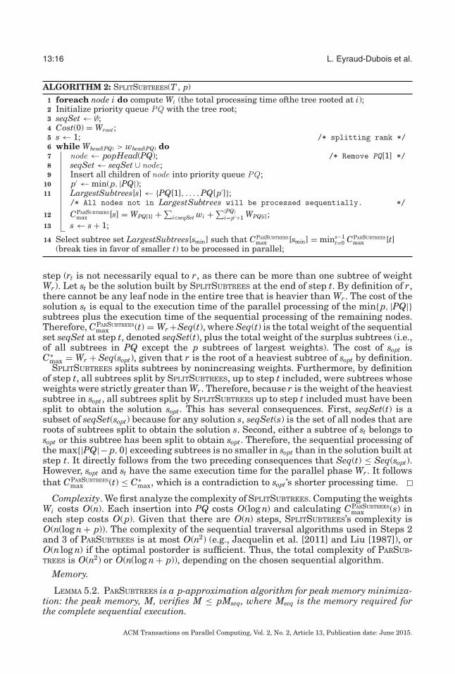
ALGORITHM 2: SPLITSUBTREES(T , p)1 foreach node i do compute Wi (the total processing time ofthe tree rooted at i);2 Initialize priority queue PQ with the tree root;3 seqSet ← ∅;4 Cost(0) = Wroot;5 s ← 1; /* splitting rank */6 while Whead(PQ) > whead(PQ) do7 node ← popHead(PQ); /* Remove PQ[1] */8 seqSet ← seqSet ∪ node;9 Insert all children of node into priority queue PQ ;
10 p′ ← min(p, |PQ|);11 LargestSubtrees[s] ← {PQ[1], . . . , PQ[p′]};
/* All nodes not in LargestSubtrees will be processed sequentially. */
12 CPARSUBTREESmax [s] = WPQ[1] + ∑
i∈seqSet wi + ∑|PQ|i=p′+1 WPQ[i];
13 s ← s + 1;
14 Select subtree set LargestSubtrees[smin] such that CPARSUBTREESmax [smin] = mins−1
t=0 CPARSUBTREESmax [t]
(break ties in favor of smaller t) to be processed in parallel;
step (rt is not necessarily equal to r, as there can be more than one subtree of weightWr). Let st be the solution built by SPLITSUBTREES at the end of step t. By definition of r,there cannot be any leaf node in the entire tree that is heavier than Wr. The cost of thesolution st is equal to the execution time of the parallel processing of the min{p, |PQ|}subtrees plus the execution time of the sequential processing of the remaining nodes.Therefore, CPARSUBTREES
max (t) = Wr +Seq(t), where Seq(t) is the total weight of the sequentialset seqSet at step t, denoted seqSet(t), plus the total weight of the surplus subtrees (i.e.,of all subtrees in PQ except the p subtrees of largest weights). The cost of sopt isC∗
max = Wr + Seq(sopt), given that r is the root of a heaviest subtree of sopt by definition.SPLITSUBTREES splits subtrees by nonincreasing weights. Furthermore, by definition
of step t, all subtrees split by SPLITSUBTREES, up to step t included, were subtrees whoseweights were strictly greater than Wr. Therefore, because r is the weight of the heaviestsubtree in sopt, all subtrees split by SPLITSUBTREES up to step t included must have beensplit to obtain the solution sopt. This has several consequences. First, seqSet(t) is asubset of seqSet(sopt) because for any solution s, seqSet(s) is the set of all nodes that areroots of subtrees split to obtain the solution s. Second, either a subtree of st belongs tosopt or this subtree has been split to obtain sopt. Therefore, the sequential processing ofthe max{|PQ|− p, 0} exceeding subtrees is no smaller in sopt than in the solution built atstep t. It directly follows from the two preceding consequences that Seq(t) ≤ Seq(sopt).However, sopt and st have the same execution time for the parallel phase Wr. It followsthat CPARSUBTREES
max (t) ≤ C∗max, which is a contradiction to sopt ’s shorter processing time.
Complexity. We first analyze the complexity of SPLITSUBTREES. Computing the weightsWi costs O(n). Each insertion into PQ costs O(log n) and calculating CPARSUBTREES
max (s) ineach step costs O(p). Given that there are O(n) steps, SPLITSUBTREES’s complexity isO(n(log n + p)). The complexity of the sequential traversal algorithms used in Steps 2and 3 of PARSUBTREES is at most O(n2) (e.g., Jacquelin et al. [2011] and Liu [1987]), orO(n log n) if the optimal postorder is sufficient. Thus, the total complexity of PARSUB-TREES is O(n2) or O(n(log n + p)), depending on the chosen sequential algorithm.
Memory.
LEMMA 5.2. PARSUBTREES is a p-approximation algorithm for peak memory minimiza-tion: the peak memory, M, verifies M ≤ pMseq, where Mseq is the memory required forthe complete sequential execution.
ACM Transactions on Parallel Computing, Vol. 2, No. 2, Article 13, Publication date: June 2015.

Parallel Scheduling of Task Trees with Limited Memory 13:17
Fig. 6. PARSUBTREES is at best a p-approximation for the makespan.
PROOF. We first note that during the parallel part of PARSUBTREES, the total memoryused, Mp, is not more than p times Mseq. Indeed, each of the p processors executesa maximal subtree, and the processing of any subtree does not use, obviously, morememory (if done optimally) than the processing of the whole tree. Thus, Mp ≤ p · Mseq.
During the sequential part of PARSUBTREES, the memory used, MS, is bounded byMseq + ∑
i∈Q fi, where the second term is for the output files produced by the root nodesof the q ≤ p subtrees processed in parallel (Q is the set of the root nodes of the qtrees processed in parallel). We now claim that at least two of those subtrees havea common parent. More specifically, let us denote by X the node that was split last(i.e., it was split in the step smin, which is selected at the end of SPLITSUBTREES). Ourclaim is that at least two children of X are processed in the parallel part. Before Xwas split (in step smin − 1), the makespan as computed in Step 12 of SPLITSUBTREES
is Cmax(smin − 1) = WX + Seq(smin − 1), where Seq(smin − 1) is the work computed insequential (
∑i∈seqSet wi + ∑|PQ|
i=PQ[p′+1] Wi). Let D denote the set of children of X that arenot executed in parallel, then the total weight of their subtrees is WD = ∑
i∈D Wi. Wenow show that if at most one child of X is processed in the parallel part, X was not thenode that was split last:
—If exactly one child C of X is processed in the parallel part, then Cmax(smin) = WX′ +Seq(smin − 1) + wX + WD, where X′ is the new head of the queue, and thus verifiesWX′ ≥ WC . And since WX = wX + WC + WD, we can conclude that Cmax(smin) ≥Cmax(smin − 1).
—If no child of X is processed in the parallel part, then Cmax(smin) = WX′ + Seq(smin −1)−WY +wX+WD, where X′ is the new head of the queue and Y is the newly insertednode in the p largest subtrees in the queue. Since WX′ ≥ WY and WX = wX + WD, weobtain once again Cmax(smin) ≥ Cmax(smin − 1).
In both cases, we have Cmax(smin) ≥ Cmax(smin − 1), which contradicts the definition ofX (the select phase, Step 2 of SPLITSUBTREES, would have selected step smin − 1 ratherthan step smin). Let us now denote by C1 and C2 two children of X that are processedin the parallel phase. Remember that the memory used during the sequential part isbounded by MS ≤ Mseq + fC1 + fC2 + ∑
i∈Q\{C1,C2} fi. Since a sequential execution mustprocess node X, we obtain fC1 + fC2 ≤ Mseq. And since ∀i, fi ≤ Mseq, we can bound thememory used during the sequential part by MS ≤ 2Mseq + (p − 2)Mseq ≤ pMseq.
Furthermore, given that up to p processors work in parallel, each on its own subtree,it is easy to see that this bound is tight if the sequential peak memory can be reachedin each subtree.
Makespan. PARSUBTREES delivers a p-approximation algorithm for makespan mini-mization, and this bound is tight. Because at least one processor is working at anytime under PARSUBTREES, PARSUBTREES delivers, in the worst case, a p-approximationfor makespan minimization. To prove that this bound is tight, we consider a tree ofheight 1 with p · k leaves (a fork), where all execution times are equal to 1 (∀i ∈ T ,wi = 1), and where k is a large integer (this tree is depicted in Figure 6). The optimalmakespan for such a tree is C∗
max = kp/p + 1 = k + 1 (the leaves are processed in
ACM Transactions on Parallel Computing, Vol. 2, No. 2, Article 13, Publication date: June 2015.

13:18 L. Eyraud-Dubois et al.
Fig. 7. No memory bound for PARSUBTREESOPTIM.
parallels, in batches of size p, and then the root is processed). With PARSUBTREES, pleaves are processed in parallel, then the remaining nodes are processed sequentially.The makespan is thus Cmax = (1 + pk− p) + 1 = p(k− 1) + 2. When k tends to +∞, theratio between the makespans tends to p.
Optimization. Given the just observed worst case for the makespan, a makespanoptimization for PARSUBTREES is to allocate all produced subtrees to the p processorsinstead of only p subtrees. This can be done by ordering the subtrees by nonincreasingtotal weight and allocating each subtree in turn to the processor with the lowest totalweight. Each of the parallel processors executes its subtrees sequentially. This opti-mized form of the algorithm is named PARSUBTREESOPTIM. Note that this optimizationshould improve the makespan, but it will likely worsen the peak memory usage.
Indeed, we can prove that PARSUBTREESOPTIM does not have an approximation ratiowith respect to memory usage. Consider the tree depicted in Figure 7, assuming thepebble-game model, to be scheduled on p processors. This tree has k levels with p − 1leaves at each level, and an additional level with p chains of length 2, and includes atotal of (k + 2)p + 1 nodes. The algorithm SPLITSUBTREES will split the subtrees rootedat a1, then a2, and so forth, until it reaches ak+1, and then b1, . . . , bp. We first prove thatSPLITSUBTREES will select a splitting where ak+1 is split. By contradiction, assume thisis not the case—in other words, the selected splitting contains a subtree rooted at ajamong the LargestSubtrees. This is obviously the largest subtree, and only p − 1 othersubtrees can be processed in parallel in PARSUBTREES, each of them contains a singleleaf. Thus, the makespan of this splitting is (k + 1)p + 2. On the contrary, splittingthe subtree rooted at ak+1 (but not the ones below) provides a solution with makespankp + 3, which is smaller as soon as p ≥ 2. Thus, SPLITSUBTREES selects a splitting thatsplits the subtree rooted at ak+1.
Furthermore, the optimal memory usage to compute this tree is p+1 (this is achievedwith a sequential postorder traversal scheduling the tree from right to left). PARSUB-TREESOPTIM schedules all leaves l j
i in parallel on all p processors, and the internal nodesa1, . . . , ak are started only once all of these leaves are finished. After completing all ofthe leaves, the memory usage is at least k(p − 1). When k tends to +∞, the ratiobetween the memory requirements also tends to +∞.
5.2. List Scheduling Algorithms
PARSUBTREES is a high-level algorithm employing sequential memory-optimizedalgorithms. An alternative, explored in this section, is to design algorithms thatdirectly work on the tree in parallel. We first present two such algorithms that are
ACM Transactions on Parallel Computing, Vol. 2, No. 2, Article 13, Publication date: June 2015.

Parallel Scheduling of Task Trees with Limited Memory 13:19
event-based list scheduling algorithms [Hwang et al. 1989]. One of the strong pointsof list scheduling algorithms is that they are (2 − 1
p)-approximation algorithms formakespan minimization [Graham 1966].
Algorithm 3 outlines a generic list scheduling, driven by node finish time events.At each event at least one node has finished, so at least one processor is available forprocessing nodes. Each available processor is given the respective head node of thepriority queue. The priority of nodes is given by the total order O, a parameter toAlgorithm 3.
ALGORITHM 3: List scheduling(T , p, O)1 Insert leaves in priority queue PQ according to order O;2 eventSet ← {0}; /* ascending order */3 while eventSet �= ∅ do /* event: node finishes */4 t ← popHead(eventSet);5 NewReadyNodes ← set of nodes whose last children completed at time t;6 Insert nodes from NewReadyNodes in PQ according to order O;7 P ← available processors at time t;8 while P �= ∅ and PQ �= ∅ do9 proc ← popHead(P);
10 node ← popHead(PQ);11 Assign node to proc;12 eventSet ← eventSet ∪ finishTime(node);
5.2.1. Heuristic PARINNERFIRST. From the study of the sequential case, one knows that apostorder traversal, while not optimal for all instances, provides good results [Jacquelinet al. 2011]. Our intention is to extend the principle of postorder traversal to the parallelprocessing. For the first heuristic, called PARINNERFIRST, the priority queue uses thefollowing ordering O: (1) inner nodes in an arbitrary order, and (2) leaf nodes orderedaccording to a given postorder traversal. Although any postorder may be used to orderthe leaves, it makes heuristic sense to choose an optimal sequential postorder so thatmemory consumption can be minimized (this is what is done in the experimentalevaluation discussed later). We do not further define the order of inner nodes, as ithas absolutely no impact. Indeed, because we target the processing of tree-shaped taskgraphs, the processing of a node makes at most one new inner node available, and theprocessing of this new inner node can start right away on the processor that freed it bycompleting the processing of its last unprocessed child.
Complexity. The complexity of PARINNERFIRST is that of determining the input or-der O and that of the list scheduling. Computing the optimal sequential postorder isO(n log n) [Liu 1986]. In the list scheduling algorithm, there are O(n) events and nnodes are inserted and retrieved from PQ. An insertion into PQ costs O(log n), so thelist scheduling complexity is O(n log n). Hence, the total complexity is also O(n log n).
Memory. PARINNERFIRST is not an approximation algorithm with respect to peak mem-ory usage. This is derived considering the tree in Figure 8. All output files have size 1,and the execution files have size 0 (∀i ∈ T : fi = 1, ni = 0). Under an optimal sequentialprocessing, leaves are processed in a deepest first order. The resulting optimal memoryrequirement is Mseq = p + 1, reached when processing a join node. With p processors,all leaves have been processed at the time the first join node (k − 1) can be executed.(The longest chain has length 2k− 2.) At that time, there are (k− 1) · (p− 1) + 1 files inmemory. When k tends to +∞, the ratio between the memory requirements also tendsto +∞.
ACM Transactions on Parallel Computing, Vol. 2, No. 2, Article 13, Publication date: June 2015.

13:20 L. Eyraud-Dubois et al.
Fig. 8. No memory bound for PARINNERFIRST.
Fig. 9. Tree with long chains.
5.2.2. Heuristic PARDEEPESTFIRST. The previous heuristic, PARINNERFIRST, tries to takeadvantage of the memory performance of optimal sequential postorders. Going in theopposite direction, another heuristic objective can be the minimization of the makespan.For trees, an inner node depends on all nodes in the subtree it defines. Therefore,it makes heuristic sense to try to process the deepest nodes first to try to reduceany possible waiting time. For the parallel processing of a tree, the most meaningfuldefinition of the depth of a node i is the w-weighted length of the path from i to the rootof the tree, including wi (therefore, the depth of node i is equal to its top-level plus wi[Casanova et al. 2008]). A deepest node in the tree is a deepest node in a critical pathof the tree.
PARDEEPESTFIRST is our proposed list scheduling deepest-first heuristic. PARDEEPEST-FIRST is defined by Algorithm 3, called with the following node ordering O: nodes areordered according to their depths, and in case of ties, inner nodes have priority overleaf nodes; remaining ties are broken according to an optimal sequential postorder.
Complexity. The complexity is the same as for PARINNERFIRST, namely O(n log n). SeePARINNERFIRST’s complexity analysis.
Memory. The memory required by PARDEEPESTFIRST is unbounded with respect tothe optimal sequential memory Mseq. Consider the tree in Figure 9 with many longchains, assuming the pebble-game model (i.e., ∀i ∈ T : fi = 1, ni = 0, wi = 1). The
ACM Transactions on Parallel Computing, Vol. 2, No. 2, Article 13, Publication date: June 2015.

Parallel Scheduling of Task Trees with Limited Memory 13:21
optimal sequential memory requirement is 3. The memory usage of PARDEEPESTFIRST
will be proportional to the number of leaves, because they are all at the same depth,the deepest one. As we can build a tree like the one in Figure 9 for any predefinednumber of chains, the ratio between the memory required by PARDEEPESTFIRST and theoptimal one is unbounded.
5.3. Memory-Constrained Heuristics
From the analysis of the three algorithms presented so far, we have seen that onlyPARSUBTREES gives a guaranteed bound on the required peak memory. The memorybehavior of the two other algorithms, PARINNERFIRST and PARDEEPESTFIRST, will be an-alyzed in the experimental evaluation presented in Section 6. In a practical setting,it might be very desirable to have a strictly bounded memory consumption to be cer-tain that the algorithm can be executed with the available limited memory. In fact,a guaranteed upper limit might be more important than a good average behavior, asthe system needs to be equipped with sufficient memory for the worst case. PARSUB-TREES’s guarantee of at most p times the optimal sequential memory seems high, andthus an obvious goal would be to have a heuristic that minimizes the makespan whilekeeping the peak memory usage below a given bound. To approach this goal, we firststudy how to limit the memory consumption of PARINNERFIRST and PARDEEPESTFIRST.Our study relies on some reduction property on trees, presented in Section 5.3.1, wherewe also show how to transform any tree into one that satisfies the reduction property.We then develop memory-constrained versions of PARINNERFIRST and PARDEEPESTFIRST
(Section 5.3.2). The memory bounds achieved by these new variants are rather lax.Therefore, we design our last heuristic, MEMBOOKINGINNERFIRST, with stronger memoryproperties (Section 5.3.3). In the experimental section (Section 6), we will show thatthese three heuristics achieve different trade-offs between makespan and memoryusage.
5.3.1. Simplifying Tree Properties. To design our memory-constrained heuristics, wemake two simplifying assumptions. First, the considered trees do not have any ex-ecution files. In other words, we assume that for any task i, ni = 0.
Eliminating execution files. To still be able to deal with general trees, we can trans-form any tree T with execution files into a strictly equivalent tree T ′ where all executionfiles have a null size. Let i be any node of T . We add to i a new leaf child i′, whoseexecution time is null (wi′ = 0), whose execution file is of null size (ni′ = 0), and whoseoutput file has size ni (fi′ = ni). Then, we set ni to 0. Any schedule S for the originaltree T can be easily transformed into a schedule S′ for the new tree T ′ with the exactsame memory and execution-time characteristics: S′ schedules a node from T at thesame time than S, and a node i from T ′ \ T at the same time than the father of i isscheduled by S (because i has a null execution time).
The second simplifying assumption is that all considered trees are reduction trees.
Definition 5.3 (Reduction Tree). A task tree is a reduction tree if the size of the outputfile of any inner node i is not more than the sum of its input files:
fi ≤∑
j∈Children(i)
f j . (1)
This reduction property is very useful, because it implies that executing an innernode does not increase the amount of memory needed (this will be used, for instance,later in Theorem 5.4).
ACM Transactions on Parallel Computing, Vol. 2, No. 2, Article 13, Publication date: June 2015.

13:22 L. Eyraud-Dubois et al.
For convenience, we sometimes use the following notation to denote the sum of thesizes of the input files of an inner node i:
inputs(i) =∑
j∈Children(i)
f j .
We now show how general trees can be transformed into reduction trees.
Turning trees into reduction trees. We can transform any tree T that does not satisfythe reduction property stated by Equation (1) into a tree where each (inner) nodesatisfies it. Let i be any inner node of T . We add to i a new leaf child i′, whoseexecution time is null (wi′ = 0), whose execution file is of null size (ni′ = 0), and whoseoutput file has the following size:
fi′ = max
⎧⎨⎩0, fi −
⎛⎝ ∑
j∈Children(i)
f j
⎞⎠
⎫⎬⎭ = max{0, fi − inputs(i)}.
The new tree is not equivalent to the original one. Let us consider an inner node ithat did not satisfy the reduction property. Then, fi′ = fi − inputs(i) > 0. The memoryused to execute node i in the tree T is inputs(i) + ni + fi. In the new tree, the memoryneeded to execute this node is (inputs(i) + (fi − inputs(i)) + ni + fi > inputs(i) + ni + fi.Any schedule of the original tree can be transformed into a schedule of the new treewith an increase of the memory usage bounded by
p × maxi
{0, fi − inputs(i)}.
Obviously, a more clever approach is to transform a tree first into a tree withoutexecution files and then to transform the new tree into a tree with the reductionproperty. Under this approach, the increase of the memory usage is bounded by
p × maxi
{0, fi − inputs(i) − ni}.
Transforming schedules. The algorithms proposed in the following sections produceschedules for reduction trees without execution files, which might have been createdfrom general trees that do not possess our simplifying properties. The schedule S′produced by an algorithm for a reduction tree without execution files T ′ can readily betransformed into a schedule S for the original tree T . To create schedule S, we simplyremove all (leaf) nodes from the schedule S′ that were introduced in the simplificationtransform (i′ ∈ T ′ \ T ). Because those nodes have zero processing time (∀i′ ∈ T ′ \ T :wi′ = 0), there is no impact on the ordering and on the starting time of the other nodesof T . In terms of memory consumption, the peak memory for schedule S is never higherthan that for schedule S′. A leaf i′ that was added to eliminate an execution file mightuse memory earlier in S′ than the execution file ni in S, but it is the same amountand freed at the same time. In terms of leaf nodes introduced to enforce the reductionproperty, they might only increase the memory needed for tree T ′ (as discussed earlier);hence, removing these nodes cannot increase the peak memory needed for schedule S.In summary, the schedule S for tree T has the same makespan as S′ and a peakmemory that is not greater than that of S′.
5.3.2. Memory-Constrained PARINNERFIRST and PARDEEPESTFIRST. Both PARINNERFIRST andPARDEEPESTFIRST are based on the list scheduling approach presented in Algorithm 3.To achieve a memory-constrained version of these algorithms for reduction trees, wemodify Algorithm 3 to obtain Algorithm 4. The code common to both algorithms isshown in gray in Algorithm 4, and the new code is printed in black.
ACM Transactions on Parallel Computing, Vol. 2, No. 2, Article 13, Publication date: June 2015.

Parallel Scheduling of Task Trees with Limited Memory 13:23
We use the same event concept as previously. However, we only start processing anode if (1) it is an inner node, or (2) it is a leaf node and the current memory consumptionplus the leaf ’s output file (fc) is less than the amount M of available memory. Once anode is encountered that fulfills neither of these conditions, the node assignment isstopped (P ← ∅) until the next event. Therefore, Algorithm 4 may deliberately keepsome processors idle when there are available tasks and thus does not necessarilyproduce a list schedule (hence, the name of “pseudo” list schedules). Subsequently, theonly approximation guarantee on the makespan produced by these heuristics is thatthey are p-approximations, the worst case for heuristics that always use at least oneprocessor at any time before the entire processing completes.
Algorithm 4 may be executed with any sequential node ordering O and any memorybound M as long as the peak memory usage of the corresponding sequential algo-rithm with the same node order O is no greater than M. From Algorithm 4, we designtwo new heuristics: PARINNERFIRSTMEMLIMIT and PARDEEPESTFIRSTMEMLIMIT. PARINNER-FIRSTMEMLIMIT uses, for the order O, an optimal sequential postorder with respect topeak memory usage. For PARDEEPESTFIRSTMEMLIMIT, nodes are ordered by nonincreas-ing depths, and in case of ties, inner nodes have priority over leaf nodes; remaining tiesare broken according to an optimal sequential postorder.
ALGORITHM 4: Pseudo list scheduling with memory limit (T , p, O, M)1 Insert leaves in priority queue PQ according to order O;2 eventSet ← {0}; /* ascending order */3 Mused ← 0; /* amount of memory used */4 while eventSet �= ∅ do /* event: node finishes */5 t ← popHead(eventSet);6 NewReadyNodes ← set of nodes whose last children completed at time t;7 Insert nodes from NewReadyNodes in PQ according to order O;8 P ← available processors at time t;9 Done ← nodes completed at time t;
10 Mused ← Mused − ∑j∈Done inputs( j);
11 while P �= ∅ and PQ �= ∅ do12 c ← head(PQ);13 if |Children(c)| > 0 or Mused + fc ≤ M then14 Mused ← Mused + fc;15 proc ← popHead(P);16 node ← popHead(PQ);17 Assign node to proc;18 eventSet ← eventSet ∪ f inishT ime(node);
19 else20 P ← ∅
THEOREM 5.4. The peak memory requirement of Algorithm 4 for a reduction treewithout execution files processed with a memory bound M and a node order O is at most2M, if M ≥ Mseq, where Mseq is the peak memory usage of the corresponding sequentialalgorithm with the same node order O.
PROOF. We first show that the required memory never exceeds 2M and then showthat the algorithms completely process the considered tree T .
We analyze the memory usage at the time a new candidate node c is consideredfor execution (line 12 of Algorithm 4). The amount of currently used memory is thenMused = InIN + OutIN + OutLF + InIdle, where
ACM Transactions on Parallel Computing, Vol. 2, No. 2, Article 13, Publication date: June 2015.

13:24 L. Eyraud-Dubois et al.
—InIN is the size of the input files of the currently processed inner nodes,—OutIN is the size of the output files of the currently processed inner nodes,—OutLF is the size of the output files of the currently processed leaves, and—InIdle is the size of the input files stored in memory but not currently used (because
they are input files of inner nodes that are not yet ready).
There are two cases—the candidate node c can be either a leaf node or an innernode:
(1) c is a leaf node. The processing of a leaf node only starts if Mused+fc ≤ M. Therefore,the processing of a leaf node never provokes the violation of the memory bound ofM, and thus a fortiori, of a memory limit of 2M.
(2) c is an inner node. The processing of a candidate inner node always starts rightaway, regardless of the amount of available memory. When the processing of c starts,the amount of required memory becomes Mnew = InIN + OutIN + OutLF + InIdle + fc.T is by hypothesis a reduction tree. Therefore, the size of the output file fc does notexceed InIdle—that is, the size of all possible input files stored in memory rightbefore the start of the processing of inner node c, but not used at that time, becausethis includes all input files of inner node c. In addition, the total size of the outputfiles of the processed inner nodes, OutIN, cannot exceed the total size of the input filesof the processed inner nodes, InIN. Therefore, Mnew = InIN + OutIN + OutLF + InIdle +fc ≤ InIN +OutIN +OutLF +2InIdle ≤ 2InIN +OutLF +2InIdle ≤ 2(InIN +OutLF +InIdle).
So the new memory requirement Mnew is not greater than twice the memoryoccupied by all input files and all output files of leaf nodes. Because the tree is areduction tree by hypothesis, executing an inner node never increases the total sizeof all input files and all output files of leaves. This can only happen by startinga leaf, but that is not done if it would exceed the required memory M. Therefore,InIN + OutLF + InIdle never exceeds M and Mnew ≤ 2M.
We now prove that when the algorithm ends, the entire input tree has been processed.We reason by contradiction and assume that this is not the case. Ready inner nodesare processed without checking the amount of available memory. Therefore, when thealgorithm terminates without having completed the processing of the tree, eventSet isempty but some leaves have not been processed. Then, let l be the first unprocessedleaf, according to the order O. At the time Algorithm 4 terminates, it has processedexactly the same leaves as the sequential algorithm when it starts processing leaf l.Because eventSet is empty, there are no remaining ready inner nodes and no node isprocessed at the time of the algorithm termination. Because of the hypothesis thatT is a reduction tree, the amount of available memory when Algorithm 4 terminatesis not smaller than the amount of available memory under the sequential algorithmright before it starts processing leaf l. Because the sequential algorithm can processthe whole tree with a peak memory usage of Mseq ≤ M, the processing of leaf l can bestarted by Algorithm 4. This contradicts the assumption of early termination.
We define a variant PARDEEPESTFIRSTMEMLIMITOPTIM of PARDEEPESTFIRSTMEMLIMIT,and a variant PARINNERFIRSTMEMLIMITOPTIM of PARINNERFIRSTMEMLIMIT, by being moreaggressive about starting leaves. Instead of checking for the condition Mused + fc ≤ Mbefore starting a leaf node c (line 13 of Algorithm 4), it is in fact sufficient to checkthat InIN + 1
2 OutLF + InIdle + fc ≤ M (using the notation of the proof of Theorem 5.4).For Case (1) of the proof, one just needs to remark that after leaf c is started, Mnew =InIN +OutIN +OutLF + InIdle+ fc. Then, because the tree is a reduction tree, OutIN ≤ InIN.Therefore, Mnew ≤ 2InIN + OutLF + fc + InIdle ≤ 2InIN + OutLF + 2fc + 2InIdle, which, inturn, is no greater than 2M because of the new condition. The modified condition has
ACM Transactions on Parallel Computing, Vol. 2, No. 2, Article 13, Publication date: June 2015.

Parallel Scheduling of Task Trees with Limited Memory 13:25
Fig. 10. Tree used to establish the worst-case performance of most memory-constrained heuristics. Node la-bels in parentheses are processing times; edge labels are memory weights. All nodes have null-size processingfiles.
no impact on the study of Case (2), because the inequality InIN + 12 OutLF + InIdle ≤ M
is sufficient to conclude that case.
Memory. Theorem 5.4 establishes that the peak memory required by PARINNERFIRST-MEMLIMIT and PARDEEPESTFIRSTMEMLIMIT with p processors is at most twice that oftheir sequential execution (p = 1) with the same order. It should be noted that thispeak requirement Mseq does not correspond in general to the memory requirementof an optimal sequential algorithm. In particular, the sequential execution of PAR-INNERFIRSTMEMLIMIT corresponds to a postorder traversal, which is not optimal for allinstances but generally provides good results [Jacquelin et al. 2011]. We propose usingPARINNERFIRSTMEMLIMIT with a node order O that corresponds to an optimal sequen-tial postorder, such as with Liu [1986]. The memory requirement of the sequentialPARDEEPESTFIRSTMEMLIMIT is unbounded compared to the optimal sequential memoryrequirement, because the same arguments apply as the ones discussed for PARDEEPEST-FIRST in Section 5.2.2.
Makespan. We have stated that the preceding heuristics are p-approximation algo-rithms for makespan minimization. The following lemma refines this result.
LEMMA 5.5. PARINNERFIRSTMEMLIMIT and PARINNERFIRSTMEMLIMITOPTIM are both p-approximation algorithms for makespan minimization, and this bound is tight.
PROOF. At any time under PARINNERFIRSTMEMLIMIT and PARINNERFIRSTMEMLIMIT-OPTIM, there is at least one processor that is not idle and is processing a task. Therefore,both PARINNERFIRSTMEMLIMIT and PARINNERFIRSTMEMLIMITOPTIM are p-approximationalgorithms for makespan minimization. We establish that this bound is tight by study-ing the tree in Figure 10. This tree can be processed with a peak memory usage ofM. We assume that PARINNERFIRSTMEMLIMIT is called with this memory limit. The keyobservation is that in any schedule, among the three descendants of an ai node, thenodes ci and bi must be processed before the di node: otherwise, keeping in memorythe output file of size M/p of node di makes it impossible to start processing the leafnode ci because of its output file of size M. And since under PARINNERFIRSTMEMLIMIT leafnodes are processed according to a postorder traversal, the processing of the subtrees issequentialized and the overall processing takes time p(2 + k). On the other hand, withrespect to the makespan, it would be better to first sequentially process in that order c1,b1, c2, b2, . . . , cp, and bp, which would take a time 2p, and then process in parallel thedi ’s for an overall makespan of 2p+ k. Hence, in this example, the approximation ratio
ACM Transactions on Parallel Computing, Vol. 2, No. 2, Article 13, Publication date: June 2015.

13:26 L. Eyraud-Dubois et al.
of PARINNERFIRSTMEMLIMIT is no smaller than p(2+k)2p+k , which tends to p when k tends to
infinity.
We do not have a similar result for the memory-limited deepest first algorithms, asalready the sequential traversal with these algorithms (which determines the givenmemory limit) can require significantly more memory than a postorder traversal. Forthe example in Figure 10, the minimum sequential memory for a deepest first traversalis equal to pM. The additional memory buys a lot of freedom for PARDEEPESTFIRSTMEM-LIMIT and makes the comparison harder.
5.3.3. Memory Booking Heuristic MEMBOOKINGINNERFIRST. The two heuristics described inthe previous section satisfy an achievable memory bound, M, in a relaxed way: theguarantee is that they never use more than twice the memory limit. Here, we aim atdesigning a heuristic that satisfies an achievable memory bound M in the strong sense:the heuristic never uses more than a memory of M.
To achieve such a goal, we want to ensure that whenever an inner node i becomesready, there is enough memory to process it. Therefore, we book in advance somememory for its later processing. Our goal is to book as little memory as possible, and todo so as late as possible. The algorithm then relies on a sequential postorder schedule,denoted PO: for any node k in the task graph, PO(k) denotes the step at which node kis executed under PO. Let j be the last child of i to be processed. If the total size of theinput files of j is larger than (or equal to) fi, then only that last child will book somememory for node i. In this case, (part of) the memory that was used to store the inputfiles of j will be used for fi. If the total size of the input files of j is smaller than fi,then the second to last child of i will also have to book some memory for fi, and so on.The following recursive formula states the amount of memory Contrib[ j] a child j hasto book for its parent i:
Contrib[ j] = min
⎛⎜⎜⎜⎝inputs( j), fi −
∑j ′ ∈ Children(i)PO( j ′) > PO( j)
Contrib[ j ′]
⎞⎟⎟⎟⎠ .
If j is a leaf, it may also have to book some memory for its parent. However, thebehavior for leaves is quite different than for inner nodes. A leaf node cannot transfersome of the memory used for its input files (because it does not have any) to its parentfor its parent output file. Therefore, the memory booked by a leaf node may not beavailable at the time of the booking. However, this memory will eventually becomeavailable (after some inner nodes are processed); booking the memory prevents thealgorithm from starting the next leaf if it would use too much memory: this ensuresthat the algorithm completes the processing without violating the memory bound. Thecontribution of a leaf j for its parent i is
Contrib[ j] = fi −∑
j ′ ∈ Children(i)PO( j ′) > PO( j)
Contrib[ j ′].
Note that the value of Contrib for each node can be computed before starting thealgorithm in a simple tree traversal. Using these formulas, we are able to guaranteethat enough memory is booked for each inner node i:∑
j∈Children(i)
Contrib[ j] = fi.
ACM Transactions on Parallel Computing, Vol. 2, No. 2, Article 13, Publication date: June 2015.

Parallel Scheduling of Task Trees with Limited Memory 13:27
ALGORITHM 5: MEMBOOKINGINNERFIRST(T , p, PO, M)Input: tree T , number of processor p, postorder PO, memory limit M (not smaller than
the peak memory of the sequential traversal defined by PO)1 foreach node i do Booked[i] ← 0;2 Mused ← 0;3 while the whole tree is not processed do4 Wait for an event (task finish time or starting point of the algorithm);5 foreach finished non–leaf node j with parent i do6 Mused ← Mused − inputs( j);7 Booked[i] ← Booked[i] + Contrib[ j];
8 NewReadyNodes ← set of nodes whose last children completed at event;9 Insert nodes from NewReadyNodes in PQ according to order O;
10 WaitForNextTermination ← false;11 while WaitForNextTermination = false and there is an available processor Pu and PQ
is not empty do12 j ← pop(PQ);13 if j is an inner node and Mused + f j ≤ M then14 Mused ← Mused + f j ;15 Booked[ j] ← 0;16 Make Pu process j;
17 else if j is a leaf and Mused + f j + ∑k/∈Ancestors( j) Booked[k] ≤ M then
18 Mused ← Mused + f j ;19 Booked[parent of j] ← Booked[parent of j] + Contrib[ j];20 Make Pu process j;
21 else22 push( j, PQ);23 WaitForNextTermination ← true;
Using these definitions, we design a new heuristic, MEMBOOKINGINNERFIRST, which isdescribed in Algorithm 5. In this algorithm, Booked[i] denotes the amount of memorycurrently booked for the processing of an inner node i. We make use of a new notation:we denote by Ancestors(i) the set of nodes on the path from i to the root node (excludingi itself)—that is, all ancestors of i.
Note that contrarily to PARINNERFIRSTMEMLIMIT, MEMBOOKINGINNERFIRST does notguarantee that there is always enough memory available to process an inner nodei as soon as it becomes ready. This is why Lemma 5.6 only guarantees that an innernode i will eventually be processed if a leaf j with PO( j) > PO(i) is started by MEM-BOOKINGINNERFIRST. This corresponds to the case when some leaf j, which is processedafter i in the sequential postorder PO, is started earlier than i in a parallel schedule:this happens when some processor is available but task i is not ready yet, as its childrenhave not yet completed.
LEMMA 5.6. Consider any inner node i. If some leaf j with PO( j) > PO(i) has beenstarted by Algorithm 5, then at some point there will be enough memory to process i.
PROOF. By contradiction, assume that an available inner node i can neverbe processed because of memory constraints—that is, Algorithm 5 stops withoutprocessing i, and some leaf j with PO( j) > PO(i) has been started (in case ofseveral such leaves, we consider the one with largest PO( j)). Note that i cannot bea parent of j (otherwise, we would have PO(i) > PO( j)). We consider the amountA = M − Mused − ∑
k/∈Ancestors( j) Booked[k] and its evolution. Before starting j, we check
ACM Transactions on Parallel Computing, Vol. 2, No. 2, Article 13, Publication date: June 2015.
13:28 L. Eyraud-Dubois et al.
that A ≥ f j . When starting j, the amount of available memory is decreased by f j, andthus we have A ≥ 0. The following events may happen after the beginning of j:
—Some inner node u not in Ancestors( j) is terminated. Let us call v its parent. When ucompletes, Mused decreases by inputs(u), whereas Booked[v] increases by Contrib[u] ≤inputs(u). Thus, A does not decrease.
—Some inner node k not in Ancestors( j) is started. In that case, the booked memory fkis traded for used memory, and the total memory amount A is preserved.
—An inner node u in Ancestors( j) is started. In this case, the amount of availablememory may temporarily decrease. However, because of the reduction property, theamount of memory freed when u completes is not smaller than the amount of addi-tional memory temporarily used for the processing of u.
—A leaf node has completed: this modifies neither the amount of available or bookedmemory, and so A is left unchanged.
Therefore, when the algorithm stops with i available, A ≥ 0. Thus, M − Mused ≥Booked[i] = fi: there is enough memory to process i.
Using the previous lemma, we now prove Algorithm MEMBOOKINGINNERFIRST.
THEOREM 5.7. MEMBOOKINGINNERFIRST called with a postorder PO and a memorybound M processes the whole tree with memory M if M is not smaller than the peakmemory of the sequential traversal defined by PO.
PROOF. By contradiction, assume that the algorithm stops while some nodes areunprocessed. We consider two cases:
—There is at least one available unprocessed inner node i (if there are several, wechoose the one with the smallest PO value). Consider the step PO(i) when this nodei is processed in the sequential postorder schedule. At this time, the set S of theleaves processed by the sequential postorder is exactly the set of the leaves j suchthat PO( j) < PO(i). Thanks to Lemma 5.6, we know that MEMBOOKINGINNERFIRST
has not processed any leaf j with PO( j) > PO(i). Therefore, the set of the leavesprocessed by MEMBOOKINGINNERFIRST is a subset of S. Node i being available, MEM-BOOKINGINNERFIRST has processed all of the leaves in the subtree ST rooted at i.MEMBOOKINGINNERFIRST cannot start a leaf k if a leaf j with PO( j) < PO(k) has notbeen started. Therefore, any leaf that precedes any leaf of ST in the postorder hasalso been processed by MEMBOOKINGINNERFIRST. By definition of a postorder, there isno leaf that does not belong to ST that is scheduled after the first leaf of ST and be-fore i. Therefore, MEMBOOKINGINNERFIRST has processed the exact same set of leavesas the sequential postorder at step PO(i). We now prove that the same set of innernodes have been processed by both algorithms:—Assume that an inner node k has been processed by MEMBOOKINGINNERFIRST but
not by the sequential postorder at time PO(i). Since k has not yet been processedby the sequential postorder, PO(k) > PO(i). Since no leaf j with PO( j) > PO(i) hasbeen processed by MEMBOOKINGINNERFIRST, since PO(k) > PO(i), and since PO is apostorder, then k can only be a parent of i, which contradicts the fact that i is notprocessed.
—Assume that an inner node k has been processed by the sequential postorder attime PO(i) but not by MEMBOOKINGINNERFIRST. Since it has been processed beforei in the sequential postorder, PO(k) < PO(i). This node, or one of its inner nodepredecessor, must be available in MEMBOOKINGINNERFIRST (note that it cannot be aleaf, as all leaves with PO values smaller than PO(i) are already processed). Thiscontradicts the fact that i is the available inner node with smallest PO value.
ACM Transactions on Parallel Computing, Vol. 2, No. 2, Article 13, Publication date: June 2015.

Parallel Scheduling of Task Trees with Limited Memory 13:29
Thus, there is no difference in the state of the sequential postorder when it startsi and MEMBOOKINGINNERFIRST when it stops, including in the amount of availablememory. This contradicts the fact that i cannot be started because of memory issues.
—There is no unprocessed available inner node. Thus, some leaf is available and cannotbe processed. Let j be the first of these leaves according to PO. None of the inner nodesfor which some memory has been booked is available, and thus they are all parents ofj (because PO is a postorder and because the processing of all leaves that precede j inPO has been completed). Thus, the memory condition that prevents j to be executedcan be rewritten: M − Mused < f j . However, since no inner node is available, this isthe same situation as right before j is processed in the sequential postorder, whichcontradicts the fact that j can be processed in the sequential postorder.
LEMMA 5.8. MEMBOOKINGINNERFIRST is a p-approximation algorithm for makespanminimization, and this bound is tight.
This result is proved following the exact same arguments than for the bound on theperformance of PARINNERFIRSTMEMLIMIT, including the tree in Figure 10.
Complexity. Algorithm 5 can be implemented with the same complexity as the otherheuristics, namely O(n log(n)) (which comes from the management of the PQ queue).The only operations added to this algorithm that could increase this complexity isthe test executed on line 17 to make sure that a new leaf can be started—that is,the computation of
∑k/∈Ancestors( j) Booked[k] for each leaf might take O(n2) time if not
done carefully. However, it is possible to avoid recomputing the values too many times.We first note the following property: when leaf j has not been started,∑
k/∈Ancestors( j)
Booked[k] =∑
PO(k)<PO( j)
Booked[k].
Indeed, if leaf j has not been started, the postorder property ensures that any k /∈Ancestors( j) with PO(k) ≥ PO( j) has Booked[k] = 0, because none of its children havestarted their execution.
For an efficient implementation, we keep a record of R = ∑PO(k)<PO( j) Booked[k] for
the leaf j that was tested on the last execution of line 17. To keep this record, it isenough to
—decrease R by Booked[i] each time an inner node i with PO(i) < PO( j) beginsexecution,
—increase R by Contrib[i] each time an inner node i with PO(i) < PO( j) finishes,—and increase R by
∑PO( j)≤PO(k)<PO( j ′) Booked[k] if a new leaf j ′ is being considered in
the test of line 17.
In total, the number of updates to R over the course of the whole algorithm isbounded by 2n: each Contrib value is added at most once to R, and each Bookedvalue is subtracted at most once. Furthermore, the cost of computing the sums∑
PO( j)≤PO(k)<PO( j ′) Booked[k] is also bounded by n since each node is considered onlyonce. Hence, these updates do not increase the total complexity of O(n log(n)) of thewhole algorithm.
6. EXPERIMENTAL VALIDATION
In this section, we experimentally compare the heuristics proposed in the previoussection and compare their performance to lower bounds.
ACM Transactions on Parallel Computing, Vol. 2, No. 2, Article 13, Publication date: June 2015.

13:30 L. Eyraud-Dubois et al.
Table I. Approximation Ratios of the Different Heuristics
Approximation Ratios with Respect toHeuristics Memory MakespanPARSUBTREES ≤ p = pPARSUBTREESOPTIM +∞ ≤ pPARINNERFIRST +∞ = 2 − 1
p
PARDEEPESTFIRST +∞ = 2 − 1p
PARINNERFIRSTMEMLIMIT ≤ 2 × MMopt
= p
PARINNERFIRSTMEMLIMITOPTIM ≤ 2 × MMopt
= p
PARDEEPESTFIRSTMEMLIMIT ≤ 2 × MMopt
≤ p
PARINNERFIRSTMEMLIMITOPTIM ≤ 2 × MMopt
≤ p
MEMBOOKINGINNERFIRST = MMopt
= p
Note: “≤ α” and “= α” mean that the heuristic is an α-approximation algo-rithm; the second expression means that the bound is tight. For memory-constrained heuristics, the ratio is expressed as a function of the optimalpeak memory Mopt and of the memory budget M. M is, by assumption,greater than the peak memory usage of the order O used by the studiedheuristic (M ≥ Mseq ≥ Mopt).
6.1. Setup
All heuristics have been implemented in C. Special care has been devoted to the im-plementation to avoid complexity issues. Especially, priority queues have been imple-mented using binary heap to allow for O(log n) insertion and minimum extraction. Wehave also implemented Liu’s algorithm [Liu 1987] to obtain the minimum sequentialmemory peak, which is used as a lower bound on memory for comparing the heuristics.
6.2. Dataset
The dataset contains assembly trees of a set of sparse matrices obtained from the Uni-versity of Florida Sparse Matrix Collection (http://www.cise.ufl.edu/research/sparse/matrices/). The chosen matrices satisfy the following assertions: not binary, not corre-sponding to a graph, square, having a symmetric pattern, a number of rows between20,000 and 2,000,000, a number of nonzeros per row at least equal to 2.5, and a num-ber of nonzeros at most equal to 5,000,000; each chosen matrix has the largest numberof nonzeros among the matrices in its group satisfying the previous assertions. Withthese criteria, we automatically select a set of medium to large matrices from differentapplication domains with a nontrivial number of nonzeros. At the time of testing, therewere 76 matrices satisfying these properties. We first order the matrices using MeTiS[Karypis and Kumar 1998] (through the MeshPart toolbox [Gilbert et al. 1998]) andamd (available in Matlab), then build the corresponding elimination trees using thesymbfact routine of Matlab. We also perform a relaxed node amalgamation [Liu 1992]on these elimination trees to create assembly trees. We have created a large set of in-stances by allowing 1, 2, 4, and 16 (if more than 1.6×10⁵ nodes) relaxed amalgamationsper node.
At the end, we compute memory weights and processing times to accurately simulatethe matrix factorization: we compute the memory weight ni of a node as η2 + 2η(μ−1),where η is the number of nodes amalgamated, and μ is the number of nonzeros inthe column of the Cholesky factor of the matrix that is associated with the highestnode (in the starting elimination tree); the processing time wi of a node is defined as2/3η3 + η2(μ − 1) + η(μ − 1)2 (these terms corresponds to one Gaussian elimination,
ACM Transactions on Parallel Computing, Vol. 2, No. 2, Article 13, Publication date: June 2015.

Parallel Scheduling of Task Trees with Limited Memory 13:31
Table II. Proportions of Scenarios When Heuristics Reach Best (or Close to Best) Performance, and AverageDeviations from Optimal Memory and Best Achieved Makespan
Heuristic
BestMemory
(%)
Within5% ofBest
Memory(%)
NormalizedMemory
BestMakespan
(%)
Within 5%of Best
Makespan(%)
NormalizedMakespan
PARSUBTREES 81.1 85.2 2.34 0.2 14.2 1.40PARSUBTREESOPTIM 49.9 65.6 2.46 1.1 19.1 1.33PARINNERFIRST 19.1 26.2 3.79 37.2 82.4 1.07PARDEEPESTFIRST 3.0 9.6 4.13 95.7 99.9 1.04
two multiplications of a triangular η × η matrix with a η × (μ − 1) matrix, and onemultiplication of a (μ − 1) × η matrix with a η × (μ − 1) matrix). The memory weightsfi of edges are computed as (μ − 1)2.
The resulting 608 trees contains from 2,000 to 1,000,000 nodes. Their depth rangesfrom 12 to 70,000, and their maximum degree ranges from 2 to 175,000. Each heuristicis tested on each tree using p = 2, 4, 8, 16, and 32 processors. Then the memory andmakespan of the resulting schedules are evaluated by simulating a parallel execution.
6.3. Results for Heuristics without Memory Bound
The comparison of the first set of heuristics (without memory bounds) is summa-rized in Table II. It presents the fraction of the cases where each heuristic reachesthe best memory (respectively makespan) among all heuristics, or when its memory(respectively makespan) is within 5% of the best one. It also shows the average nor-malized memory and makespan. For each scenario (consisting in a tree and a numberof processors), the memory obtained by each heuristic is normalized by the optimal(sequential) memory, and the makespan is normalized using a classical lower bound,since makespan minimization is NP-hard even without memory constraint. The lowerbound is the maximum between the total processing time of the tree divided by thenumber of processors and the maximum weighted critical path.
Table II shows that PARSUBTREES and PARSUBTREESOPTIM are the best heuristicsfor memory minimization. On average, they use less than 2.5 times the amountof memory required by the optimal sequential traversal, when PARINNERFIRST andPARDEEPESTFIRST need 3.79 and 4.13 times this amount of memory, respectively.PARINNERFIRST and PARDEEPESTFIRST perform best for makespan minimization, havingmakespans very close on average to the best achieved ones, which is consistent withtheir 2-approximation ratio for makespan minimization. Furthermore, given thecritical-path–oriented node ordering, we can expect that PARDEEPESTFIRST makespan isclose to optimal. PARDEEPESTFIRST outperforms PARINNERFIRST for makespan minimiza-tion, at the cost of a noticeable increase in memory. PARSUBTREES and PARSUBTREESOPTIM
may be better trade-offs, as they use (on average) almost only half the memory ofPARDEEPESTFIRST for at most a 35% increase in makespan.
Figure 11 presents the evolution of the performance of these heuristics with thenumber of processors. The figure displays average normalized makespan and memory,and vertical bars represent 95% confidence intervals for the mean.3 On this figure, weplot the results for all 608 trees except 76 of them, for which the results are so differ-ent that it does not make sense to compute average values anymore. These outliersbelong to four different classes of applications, and the specific results for these graphsare shown in Figure 12. Note that in both figures, values of the different plots are
3The confidence intervals are obtained with the nonparametric bootstrap method.
ACM Transactions on Parallel Computing, Vol. 2, No. 2, Article 13, Publication date: June 2015.

13:32 L. Eyraud-Dubois et al.
Fig. 11. Performance (makespan and memory) to the respective lower bounds for the first set of heuristics,excluding the trees with extreme performance. Vertical bars represent 95% confidence intervals.
Fig. 12. Performance (makespan and memory) to the respective lower bounds for the first set ofheuristics for four specific classes of trees that show specific behavior (CPM: closest point method;Mulvey: closest point method; QY: transient stability-constrained interior point optimal power flow;TSOPF: transient stability-constrained optimal power flow; see details on http://www.cise.ufl.edu/research/sparse/matrices/groups.html). Vertical bars represent 95% confidence intervals.
slightly offset on the x axis for better readability. Figure 11 shows that PARDEEPEST-FIRST and PARINNERFIRST have a similar performance evolution, just like PARSUBTREES
and PARSUBTREESOPTIM. The performance gap between these two groups, both for mem-ory and makespan, increases with the number of processors. With a large number of
ACM Transactions on Parallel Computing, Vol. 2, No. 2, Article 13, Publication date: June 2015.

Parallel Scheduling of Task Trees with Limited Memory 13:33
processors, PARDEEPESTFIRST and PARINNERFIRST are able to decrease the normalizedmakespan (at the cost of an increase of memory), whereas PARSUBTREES has an almostconstant normalized makespan with the number of processors.
Despite the very different values for makespan and memory utilization, and a muchhigher variability, the results for the outliers presented in Figure 12 give the same con-clusions about the relative performance of the heuristics. Furthermore, this graph alsoexhibits the absence of approximation ratios for PARDEEPESTFIRST and PARINNERFIRST
for memory minimization. Indeed, even though the trees used in this set are takenfrom real-life applications, in contrast with the carefully crafted counterexamples ofSection 5, the memory usage of PARDEEPESTFIRST and PARINNERFIRST on those trees canreach up to 100 times the optimal memory usage.
6.4. Results for Memory-Constrained Heuristics
In addition to the previous heuristics, we also test the memory-constrained heuris-tics. Since they can be applied only to reduction trees with null processing sizes, wetransform the trees used in the previous tests into reduction trees as explained inSection 5.3.1. For a given scenario (tree, number of processors, memory bound), thememory obtained by each heuristic is normalized by the optimal memory on the orig-inal tree (not the reduction one). Thus, the normalized memory represents the actualmemory used by the heuristic compared to the one of a sequential processing. In par-ticular, this allows a fair comparison between memory-constrained heuristics and theprevious unconstrained heuristics.
To compare the memory-constrained heuristics, we have applied them on the previ-ous dataset using various memory bounds. For each tree, we first compute the minimumsequential memory Mseq obtained by a postorder traversal of the original tree. Then,each heuristic is tested on the corresponding tree with a memory bound B = xMseqfor various ratios x ≥ 1. Sometimes the heuristic cannot run because the amount ofavailable memory is too small. This is explained by the following factors:
—The memory-constrained heuristics use a reduction tree that may well need morememory than the original tree. In general, however, the transformation from theoriginal tree does not significantly increase the minimum amount of memory neededto process the tree.
—PARINNERFIRSTMEMLIMIT has a minimum memory guarantee that is twice the sequen-tial memory of a postorder traversal, and thus it cannot run with a memory smallerthan 2Mseq.
—PARDEEPESTFIRSTMEMLIMIT has a minimum memory guarantee that is twice the se-quential memory of a deepest first sequential traversal of the tree. A deepest firsttraversal uses much more memory than a postorder traversal, and thus PARDEEPEST-FIRSTMEMLIMIT needs much more memory than PARINNERFIRSTMEMLIMIT to process atree.
Figure 13 presents the results of these simulations. In this figure, points are shownonly when a heuristic succeeds in more than 95% of the cases. The intuition is that witha success rate larger than 95%, the heuristic is presumably useful for this ratio. Thisfigure shows that when the memory is very limited (B < 2Mseq), MEMBOOKINGINNERFIRST
is the only heuristic that can be run, and it achieves reasonable makespans. For a lessstrict memory bound (2Mseq ≤ B < 5Mseq or 2Mseq ≤ B < 10Mseq depending on thenumber of processors), PARINNERFIRSTMEMLIMIT is able to process the tree and achievesbetter makespans, especially when B is large. Finally, when memory is abundant,PARDEEPESTFIRSTMEMLIMIT is the best among all heuristics. In the figure, we also testedthe two variants PARINNERFIRSTMEMLIMITOPTIM and PARDEEPESTFIRSTMEMLIMITOPTIM
presented in Section 5.3.2 that are more aggressive when starting leaves, but with the
ACM Transactions on Parallel Computing, Vol. 2, No. 2, Article 13, Publication date: June 2015.

13:34 L. Eyraud-Dubois et al.
Fig
.13.
Mem
ory
and
mak
espa
npe
rfor
man
ceof
mem
ory-
con
stra
ined
heu
rist
ics
(log
arit
hm
icsc
ale)
.
ACM Transactions on Parallel Computing, Vol. 2, No. 2, Article 13, Publication date: June 2015.
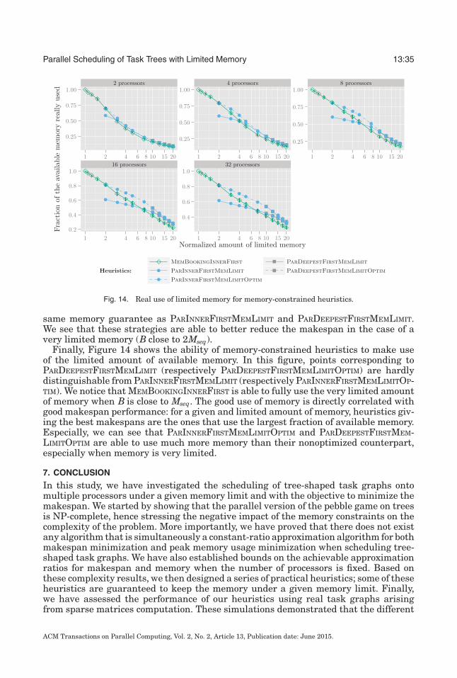
Parallel Scheduling of Task Trees with Limited Memory 13:35
Fig. 14. Real use of limited memory for memory-constrained heuristics.
same memory guarantee as PARINNERFIRSTMEMLIMIT and PARDEEPESTFIRSTMEMLIMIT.We see that these strategies are able to better reduce the makespan in the case of avery limited memory (B close to 2Mseq).
Finally, Figure 14 shows the ability of memory-constrained heuristics to make useof the limited amount of available memory. In this figure, points corresponding toPARDEEPESTFIRSTMEMLIMIT (respectively PARDEEPESTFIRSTMEMLIMITOPTIM) are hardlydistinguishable from PARINNERFIRSTMEMLIMIT (respectively PARINNERFIRSTMEMLIMITOP-TIM). We notice that MEMBOOKINGINNERFIRST is able to fully use the very limited amountof memory when B is close to Mseq. The good use of memory is directly correlated withgood makespan performance: for a given and limited amount of memory, heuristics giv-ing the best makespans are the ones that use the largest fraction of available memory.Especially, we can see that PARINNERFIRSTMEMLIMITOPTIM and PARDEEPESTFIRSTMEM-LIMITOPTIM are able to use much more memory than their nonoptimized counterpart,especially when memory is very limited.
7. CONCLUSION
In this study, we have investigated the scheduling of tree-shaped task graphs ontomultiple processors under a given memory limit and with the objective to minimize themakespan. We started by showing that the parallel version of the pebble game on treesis NP-complete, hence stressing the negative impact of the memory constraints on thecomplexity of the problem. More importantly, we have proved that there does not existany algorithm that is simultaneously a constant-ratio approximation algorithm for bothmakespan minimization and peak memory usage minimization when scheduling tree-shaped task graphs. We have also established bounds on the achievable approximationratios for makespan and memory when the number of processors is fixed. Based onthese complexity results, we then designed a series of practical heuristics; some of theseheuristics are guaranteed to keep the memory under a given memory limit. Finally,we have assessed the performance of our heuristics using real task graphs arisingfrom sparse matrices computation. These simulations demonstrated that the different
ACM Transactions on Parallel Computing, Vol. 2, No. 2, Article 13, Publication date: June 2015.

13:36 L. Eyraud-Dubois et al.
heuristics achieve different trade-offs between the minimization of peak memory usageand makespan; hence, the set of designed heuristics provide an efficient solution foreach situation.
This work represents an important step toward a comprehensive theoretical analy-sis of memory/makespan minimization for applications organized as trees of tasks, asit provides both complexity results and memory-constrained heuristics. Multifrontalsparse matrix factorization is an important application for this work and a good in-centive to refine the computation model. In a second step, we should consider trees ofparallel tasks rather than of pure sequential tasks, as the computations correspond-ing to large tasks (at the top of the tree) are usually distributed across processors.Of course, one would need a proper computation model to derive relevant complexityresults. To get even closer to reality, one would also need to consider distributed mem-ory rather than shared memory, or a mix of both. Furthermore, all of our schedulingpolicies are static, as they construct a final schedule before the computation starts. Inpractice, lightweight dynamic schedulers are needed that are able to cope with inaccu-rate timing predictions and to react to changes in the application: for example, usingnumerical pivoting will slightly alter the duration of tasks and the size of data. Hence,many important but challenging findings remain to be discovered.
ACKNOWLEDGMENTS
We thank the anonymous reviewers for their careful reading and helpful comments. We thank Bora Ucar forhis help in creating and managing the dataset used in the experiments. We gratefully acknowledge that thiswork is partially supported by the Marsden Fund Council from government funding, grant 9073-3624767,administered by the Royal Society of New Zealand, and by the ANR RESCUE and SOLHAR projects, fundedby the French National Research Agency.
REFERENCES
E. Agullo, P. Amestoy, A. Buttari, A. Guermouche, J.-Y. L’Excellent, and F.-H. Rouet. 2012. Robust memory-aware mappings for parallel multifrontal factorizations. In Proceedings of the SIAM Conference onParallel Processing for Scientific Computing (PP’12).
P. R. Amestoy, I. S. Duff, J. Koster, and J.-Y. L’Excellent. 2001. A fully asynchronous multifrontal solver usingdistributed dynamic scheduling. SIAM Journal on Matrix Analysis and Applications 23, 1, 15–41.
P. R. Amestoy, A. Guermouche, J.-Y. L’Excellent, and S. Pralet. 2006. Hybrid scheduling for the parallelsolution of linear systems. Parallel Computing 32, 2, 136–156.
H. Casanova, A. Legrand, and Y. Robert. 2008. Parallel Algorithms. Chapman and Hall, London, UK.T. A. Davis. 2006. Direct Methods for Sparse Linear Systems. Society for Industrial and Applied Mathematics,
Philadelphia, PA.M. R. Garey and D. S. Johnson. 1979. Computers and Intractability, A Guide to the Theory of NP-Completeness.
W. H. Freeman and Co, London, UK.J. R. Gilbert, T. Lengauer, and R. E. Tarjan. 1980. The pebbling problem is complete in polynomial space.
SIAM Journal on Computing 9, 3, 513–524.J. R. Gilbert, G. L. Miller, and S.-H. Teng. 1998. Geometric mesh partitioning: Implementation and experi-
ments. SIAM Journal on Scientific Computing 19, 6, 2091–2110.R. L. Graham. 1966. Bounds for certain multiprocessing anomalies. Bell System Technical Journal XLV, 9,
1563–1581.A. Guermouche and J.-Y. L’Excellent. 2004. Memory-based scheduling for a parallel multifrontal solver. In
Proceedings of the 18th International Parallel and Distributed Processing Symposium (IPDPS’04). IEEE,Los Alamitos, CA, 71–81. DOI:http://dx.doi.org/10.1109/IPDPS.2004.1303001
T. C. Hu. 1961. Parallel sequencing and assembly line problems. Operations Research 9, 6, 841–848.J. J. Hwang, Y. C. Chow, F. D. Anger, and C. Y. Lee. 1989. Scheduling precedence graphs in systems with
interprocessor communication times. SIAM Journal of Computing 18, 2, 244–257.M. Jacquelin, L. Marchal, Y. Robert, and B. Ucar. 2011. On optimal tree traversals for sparse matrix factor-
ization. In Proceedings of the 25th IEEE International Parallel and Distributed Processing Symposium(IPDPS ’11). IEEE, Los Alamitos, CA, 556–567.
ACM Transactions on Parallel Computing, Vol. 2, No. 2, Article 13, Publication date: June 2015.

Parallel Scheduling of Task Trees with Limited Memory 13:37
G. Karypis and V. Kumar. 1998. MeTiS: A Software Package for Partitioning Unstructured Graphs, Parti-tioning Meshes, and Computing Fill-Reducing Orderings of Sparse Matrices Version 4.0. University ofMinnesota, Department of Computer Science and Engineering, Army HPC Research Center, Minneapo-lis, MN.
C.-C. Lam, T. Rauber, G. Baumgartner, D. Cociorva, and P. Sadayappan. 2011. Memory-optimal evaluationof expression trees involving large objects. Computer Languages, Systems and Structures 37, 2, 63–75.
J. K. Lenstra, A. H. G. Rinnooy Kan, and P. Brucker. 1977. Complexity of machine scheduling problems.Annals of Discrete Mathematics 1, 343–362.
J. Liu. 1992. The multifrontal method for sparse matrix solution: Theory and practice. SIAM Review 34, 1,82–109. DOI:http://dx.doi.org/10.1137/1034004
J. W. H. Liu. 1986. On the storage requirement in the out-of-core multifrontal method for sparse factorization.ACM Transactions on Mathematical Software 12, 3, 249–264.
J. W. H. Liu. 1987. An application of generalized tree pebbling to sparse matrix factorization. SIAM Journalon Algebraic Discrete Methods 8, 3, 375–395.
L. Marchal, O. Sinnen, and F. Vivien. 2013. Scheduling tree-shaped task graphs to minimize memory andmakespan. In Proceedings of the 27th IEEE International Symposium on Parallel and DistributedProcessing (IPDPS’13). IEEE, Los Alamitos, CA, 839–850.
A. Ramakrishnan, G. Singh, H. Zhao, E. Deelman, R. Sakellariou, K. Vahi, K. Blackburn, D. Meyers, andM. Samidi. 2007. Scheduling data-intensive workflows onto storage-constrained distributed resources.In Proceedings of the IEEE Symposium on Cluster Computing and the Grid (CCGrid’07). IEEE, LosAlamitos, CA, 401–409.
R. Sethi. 1973. Complete register allocation problems. In Proceedings of the 5th Annual ACM Symposium onTheory of Computing (STOC’73). ACM, New York, NY, 182–195.
R. Sethi and J. D. Ullman. 1970. The generation of optimal code for arithmetic expressions. Journal of theACM 17, 4, 715–728.
Received January 2014; revised April 2015; accepted May 2015
ACM Transactions on Parallel Computing, Vol. 2, No. 2, Article 13, Publication date: June 2015.