a wavelet galerkin method for the solution of partial...
TRANSCRIPT

1
A WAVELET–GALERKIN METHOD FOR THE SOLUTION OF
PARTIAL DIFFERENTIAL EQUATION
A THESIS SUBMITED IN PARTIAL FULFILMENT OF
THE REQUIREMENT FOR THE DEGREE OF
MASTER OF SCIENCE IN MATHEMATICS
BY
ANANDITA DANDAPAT
ROLL NO-409MA2062
UNDER THE SUPERVISION OF
PROF.SANTANU SAHA RAY
DEPARTMENT OF MATHEMATICS,
NATIONAL INSTITUTE OF TECHNOLOGY
ROURKELA, ORISSA-769008

2
NATIONAL INSTITUTE OF TECHNOLOGY
ROURKELA
CERTIFICATE
This is to certify that the thesis entitled “Wavelet-Galerkin Method for the
Solution of Partial Differential Equation” submitted by Ms. Anandita
Dandapat, Roll No.409MA2062, for the award of the degree of Master of
Science from National Institute of Technology, Rourkela, is absolutely best
upon her own work under the guidance of Prof. (Dr.) S.Saha Ray. The results
embodied in this thesis are new and neither this thesis nor any part of it has been
submitted for any degree/diploma or any academic award anywhere before.
Date: Dr.S.Saha Ray
Associate Professor
Department of Mathematics
National Institute of Technology
Rourkela-769008, Orissa, India
3
DECLARATION
I declare that the topic ‘A Wavelet-Galerkin method for the Solution of
Partial Differential Equation’ for my M.Sc. degree has not been submitted in
any other institution or University for the award of any other degree or diploma.
Place: Anandita Dandapat
Date: Roll.No.409MA2062
Department of Mathematics
National Institute of Technology
Rourkela-769008
Orissa, India

4
ACKNOWLEDGEMENT
I wish to express my deep sense of gratitude to my supervisor
Dr. S. Saha Ray, Associate Professor, Department of Mathematics, National
Institute of Technology, Rourkela for his inspiring guidance and assistance in
the preparation of thesis.
I am grateful to Prof. P.C. Panda, Director, National Institute of Technology,
Rourkela for providing excellent facilities in the institute for carrying out
research.
I also take the opportunity to acknowledge quite explicitly with gratitude my
debt to the head of the Department prof. G.K.Panda and all the professors and
staff, Department of Mathematics, National Institute of Technology, Rourkela
for his encouragement and valuable suggestions during the preparation of this
thesis.
I am extremely grateful to my parents and my friends, who are a constant source
of inspiration for me.
Rourkela, 769008 Anandita Dandapat
May, 2011 Roll No-409MA2062
National Institute of Technology
Rourkela-769008
Orissa, India
5
Abstract
Wavelet function generates significant interest from both theoretical and
applied research given in the last ten years. In the present project work, the
Daubechies family of wavelets will be considered due to their useful properties.
Since the contribution of compactly supported wavelet by Daubechies and multi
resolution analysis based on Fast Fourier Transform (FWT) algorithm by
Beylkin, wavelet based solution of ordinary and partial differential equations
gained momentum in attractive way. Advantages of Wavelet-Galerkin Method
over finite difference or element method have led to tremendous application in
science and engineering.
In the present project work the Daubechies families of wavelets have been
applied to solve differential equations. Solution obtained may the Daubechies-6
coefficients has been compared with exact solution. The good agreement of
mathematical results , with the exact solution proves the accuracy and efficiency
of Wavelet-Galerkin Method.

6
CONTENTS
Chapter 1 Introduction 7
Chapter 2 Wavelet based complete coordinate function. 9
Chapter 3 Multiresolution. 13
Chapter 4 Connection coefficient. 16
Chapter 5 Singularity perturbed second-order boundary
value problem. 19
Chapter 6 Example 23
Chapter 7 Conclusion 29
Bibliography 31

7
CHAPTER-1
Introduction
Wavelet Galerkin method is useful to solve partial differential equation.
Wavelet analysis is a numerical concept which allows representing a function in
terms of a set of basis functions, called wavelets, which are localized both in
location and scale. Wavelets used in this method are mostly compact support
introduce by Daubechies [1].
The wavelet based approximations of ordinary and partial differential equations
[1-4] have been attracting the attention, since the contribution of orthonormal
bases of compactly supported wavelet by Daubechies [5] and Multiresolution
analysis based Fast Wavelet Transform Algorithm (F.W.T) by Beylkin [6]
gained momentum to make wavelet approximations attractive. Among the
wavelet approximations, the Wavelet-Galerkin technique [7-10] is the most
frequently used scheme nowadays .Wavelet based numerical solutions of partial
differential equations have been developed by several researchers [2, 3, 7, 10-
14].
Daubechies constructed a family of orthonormal bases of compactly supported
wavelets for the space of square-integrable function )(2 RL . The Wavelet-
Galerkin scheme involves the evaluation of connection coefficients are integrals
with integrands being products of wavelet bases and their derivatives.

8
Due to the derivatives of compactly supported wavelets, it is difficult and
unstable to compute the connection coefficients by the numerical evaluation of
integral. The connection coefficients and the associated computations
algorithms have been developed in [8,12] for bounded and unbounded domains.
Wavelet )(x : An oscillatory function )()( 2 RLx with zero mean is a wavelet
if it has the desirable properties:
1.Smoothness: )(x is n times differentiable and that their derivatives are
continuous.
2.Localization: )(x is well localized both in time and frequency domains, i.e.,
)(x and its derivatives must decay very rapidly. For frequency localization
)(ˆ must decay sufficiently fast as and that )(ˆ becomes flat in the
neighborhood of 0 . The flatness is associated with number of vanishing
moments of )(x , i.e.,
0)( dkxx k or equivalently 0)(ˆ k
k
d
d for nk ,......,1 ,0
in the sense that larger the number of vanishing moments more is the flatness
when is small.
3.The admissibility condition
d
2
)(ˆ
suggests that 2
)(ˆ decay at least as 1
or 1
x for 0 .

9
Chapter-2
Wavelet Based Complete coordinate Function
The Daubechies [5, 15] defined the class of compactly supported
wavelets. This means that they have non zero values within a finite interval and
have a zero value everywhere else. Let )(x be a solution of scaling relation
1
0
)2()(L
k
k kxax (1)
The expression )(x is called Scaling function. And wavelet function )(x is
)2()1()( 1
1
kxax k
Lk
k
(2)
where L is positive even integral.
From the normalization 1)(x of the scaling function, the first condition can
be written as follows,
21
0
L
k
ka (3)
The translation of )(x are required to be orthonormal

10
mkkx ,m)-(x )( (4)
This formula (4) implies the second condition
1
0
02
L
k
mmkk aa (5)
Where is the Kronecker delta function.
Smooth wavelet function requires the moment of the wavelet to be zero
0)( dxxx m (6)
This formula (6) implies the third condition
1
0
0)1(L
k
k
mk ak for 12
,....,1 ,0 Lm (7)
Figure1: Daubechies’ scaling and wavelet function for 6L .
11
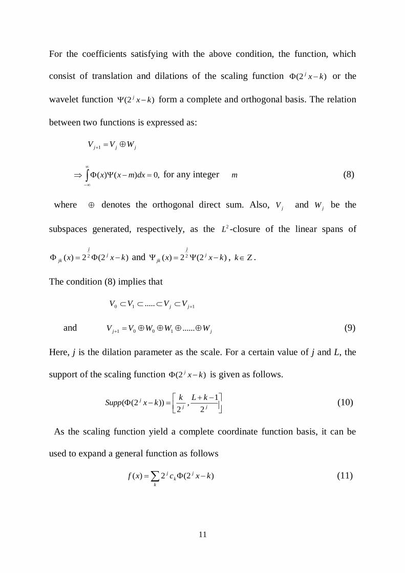
For the coefficients satisfying with the above condition, the function, which
consist of translation and dilations of the scaling function )2( kxj or the
wavelet function )2( kxj form a complete and orthogonal basis. The relation
between two functions is expressed as:
jjj WVV 1
,0)()(
dxmxx for any integer m (8)
where denotes the orthogonal direct sum. Also, jV and jW be the
subspaces generated, respectively, as the 2L -closure of the linear spans of
)2(2)( 2 kxx j
j
jk and )2(2)( 2 kxx j
j
jk , k .
The condition (8) implies that
110 ..... jj VVVV
and jj WWWVV ......1001 (9)
Here, j is the dilation parameter as the scale. For a certain value of j and L, the
support of the scaling function )2( kxj is given as follows.
jj
j kLkkxSupp
2
1,
2))2(( (10)
As the scaling function yield a complete coordinate function basis, it can be
used to expand a general function as follows
k
j
k
j kxcxf )2(2)( (11)
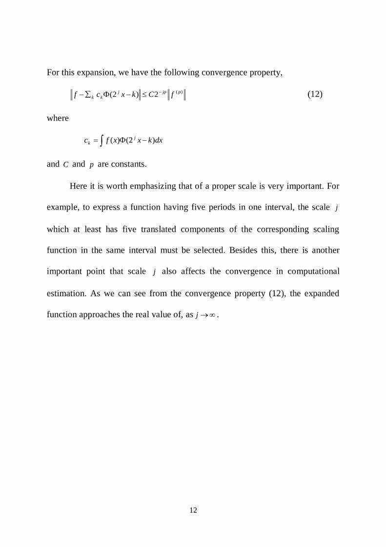
12
For this expansion, we have the following convergence property,
)(2)2( pjpj
kk fCkxcf (12)
where
dxkxxfc j
k )2()(
and C and p are constants.
Here it is worth emphasizing that of a proper scale is very important. For
example, to express a function having five periods in one interval, the scale j
which at least has five translated components of the corresponding scaling
function in the same interval must be selected. Besides this, there is another
important point that scale j also affects the convergence in computational
estimation. As we can see from the convergence property (12), the expanded
function approaches the real value of, as j .

13
CHAPTER 3
Multiresolution in )(2 RL
Multiresolution analysis is the method of most of the practically relevant
discrete wavelet transform.
A Multiresolution analysis of the space )(2 RL consist of a
sequence of closed subspace jV with the following properties:
ZjVV jj ,)1 1
1)2()()2 jj VxfVxf
00 )1()()3 VxfVxf
Zj jV
)4 is dense in 0),(2 j ZjVRL
The existence of a scaling function )(x is required to generate a basis in each
jV by
Zijij spanV
With
Zijixj
ij
j
,),2(2 2
In the classical case this basis orthonormal, so that

14
, of which the translates and dilates constitutes orthonormal
bases of the spaces jW . ,, ikRjkji
With ,)()(, dxxgxfgf
being the usual inner product.
Let the jW denote a subspace complementing the subspace jV in 1jV i.e.
jjj WVV 1 .
Each element of 1jV can be uniquely written as the sum of an element in jV ,
and an element in jW which contains the details required to pass from an
approximation at level j to an approximation at level 1j .
Based on the function )(x one can find )(x , the so-called mother wavelet
ZispanW jij
Generated by the wavelets
Zijixj
ji
j
,),2(2 2
Each function )(2 RLf , can now be expressed as
Zi
jiji
jj
ijij
Zi
xdxcxf )()()(0
00
Where RjijiRjiji fdfc ,,
The scaling function )(x and its mother wavelet )(x have the following
properties:

15
,1)( dxx
jidxixjx ,)()(
2,1,0,0)(
kdxxxk
and
0)()(
dxkxx , For any integer k
This condition implies that jjj WVV 1 on each fixed and scale j , the
wavelets Zkjk x
)( form an orthonormal basis jW and the scaling functions
Zkjk x
)( form an orthonormal basis of jV
The set of spaces of set jV is called as Multiresolution analysis of )(2 RL .These
spaces will be used to approximate the solutions of Partial Differential
Equations using the Wavelet-Galerkin method.
16
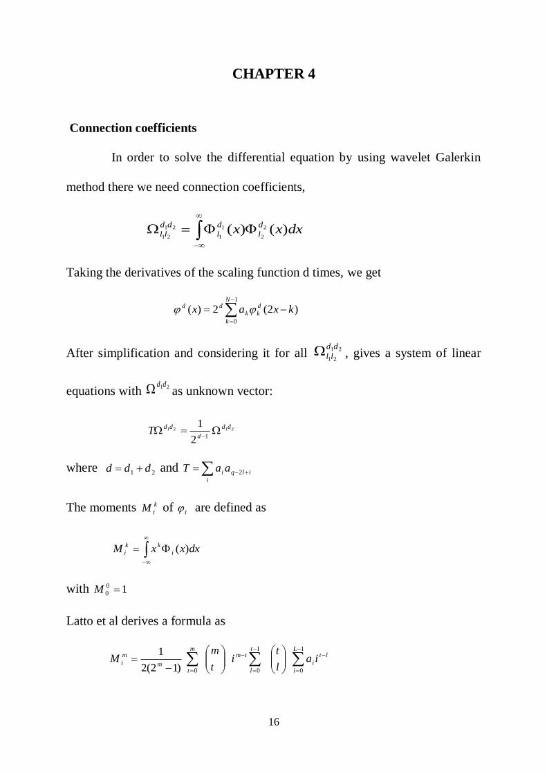
CHAPTER 4
Connection coefficients
In order to solve the differential equation by using wavelet Galerkin
method there we need connection coefficients,
dxxxd
l
d
l
dd
ll )()( 2
2
1
1
21
21
Taking the derivatives of the scaling function d times, we get
1
0
)2(2)(N
k
d
kk
dd kxax
After simplification and considering it for all 21
21
dd
ll , gives a system of linear
equations with 21dd
as unknown vector:
2121
12
1 dd
d
ddT
where 21 ddd and i
ilqi aaT 2
The moments k
iM of i are defined as
dxxxM i
kk
i )(
with 10
0 M
Latto et al derives a formula as
m
t
t
l
L
i
lt
i
tm
m
m
i ial
ti
t
mM
0
1
0
1
0
)12(2
1
17
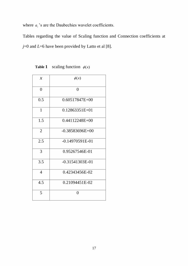
where ia ’s are the Daubechies wavelet coefficients.
Tables regarding the value of Scaling function and Connection coefficients at
j=0 and L=6 have been provided by Latto et al [8].
Table 1 scaling function )(x
x )(x
0 0
0.5 0.60517847E+00
1 0.12863351E+01
1.5 0.44112248E+00
2 -0.38583696E+00
2.5 -0.14970591E-01
3 0.95267546E-01
3.5 -0.31541303E-01
4 0.42343456E-02
4.5 0.21094451E-02
5 0

18
Table 2 : Daubechies Wavelet filter coefficients, L=6
0a 0.470467207784
1a 1.14111691583
2a 0.650365000526
3a -0.190934415568
4a -0.120832208310
5a 0.0498174997316
Table 3: Connection coefficient at 0j ,6 L dxnxkxkn )( )(][
]4[ 0.00535714285714
]3[ 0.11428571428571
]2[ -0.87619047619052
]1[ 3.39047619047638
]0[ -5.26785714285743
]1[ 3.39047619047638
]2[ -0.87619047619052
]3[ 0.11428571428571
]4[ 0.00535714285714
19
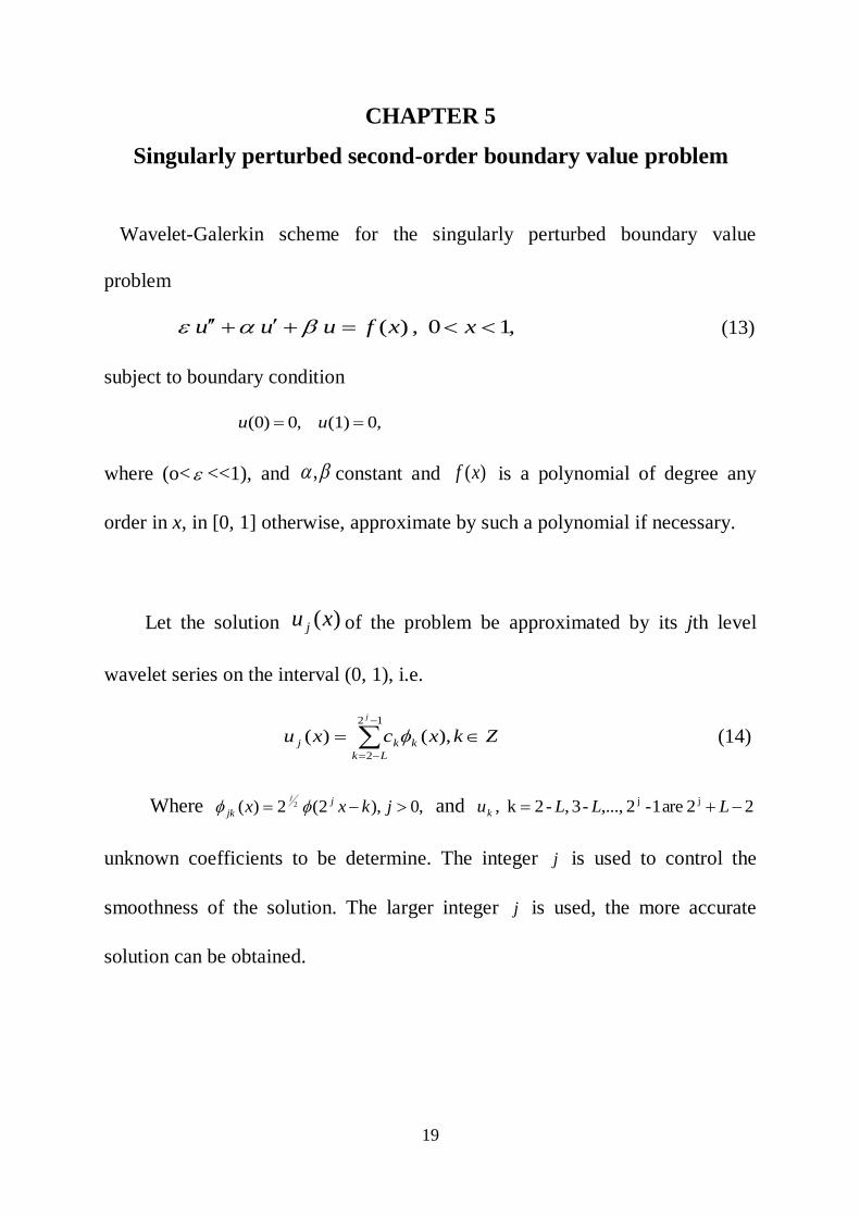
CHAPTER 5
Singularly perturbed second-order boundary value problem
Wavelet-Galerkin scheme for the singularly perturbed boundary value
problem
,1 0 , )( xxfuuu (13)
subject to boundary condition
0,(1) ,0)0( uu
where (o< <<1), and , constant and )(xf is a polynomial of degree any
order in x, in [0, 1] otherwise, approximate by such a polynomial if necessary.
Let the solution )(xu j of the problem be approximated by its jth level
wavelet series on the interval (0, 1), i.e.
12
2
),()(
j
Lk
kkj Zkxcxu (14)
Where ,0),2(2)( 2 jkxx j
jk
j
and 22 are 1-2 ,...,-3 ,-2k , jj LLLuk
unknown coefficients to be determine. The integer j is used to control the
smoothness of the solution. The larger integer j is used, the more accurate
solution can be obtained.
20
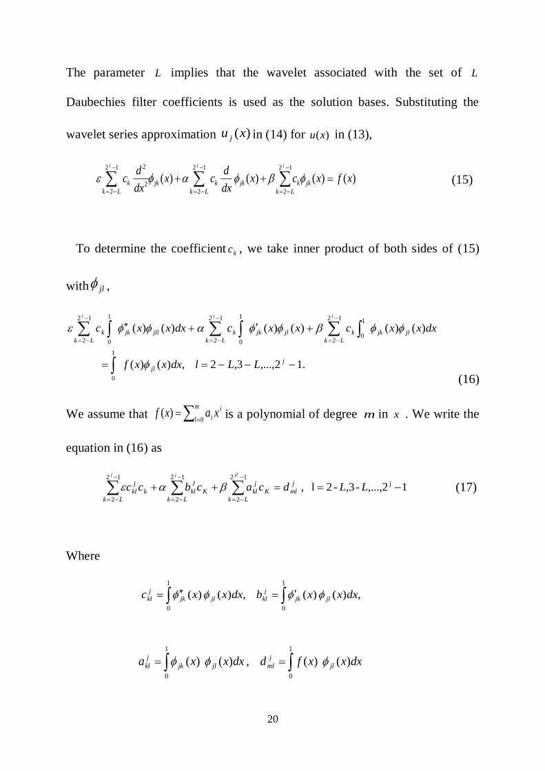
The parameter L implies that the wavelet associated with the set of L
Daubechies filter coefficients is used as the solution bases. Substituting the
wavelet series approximation )(xu j in (14) for )(xu in (13),
)()()()(12
2
12
2
12
22
2
xfxcxdx
dcx
dx
dc
jjj
Lk
jkk
Lk
jkkjk
Lk
k
(15)
To determine the coefficient kc , we take inner product of both sides of (15)
with jl ,
.12,...,3,2 ,)()(
)()()()()()(
1
0
12
2
1
0
12
2
1
0
12
2
1
0
j
jl
Lk
jljkk
Lk
jljkkjlljk
Lk
k
LLldxxxf
dxxxcxxcdxxxc
jjj
(16)
We assume that
m
l
i
i xaxf0
)( is a polynomial of degree m in x . We write the
equation in (16) as
1,...,2-,3-2l , j12
2
12
2
12
2
LLdcacbcc j
mlK
Lk
j
kl
Lk
K
J
klk
j
kl
Lk
jJjj
(17)
Where
,)( )( ,)( )(
1
0
1
0
dxxxbdxxxc jljk
j
kljljk
j
kl
1
0
1
0
)( )( , )( )(
dxxxfddxxxa jl
j
mljljk
j
kl
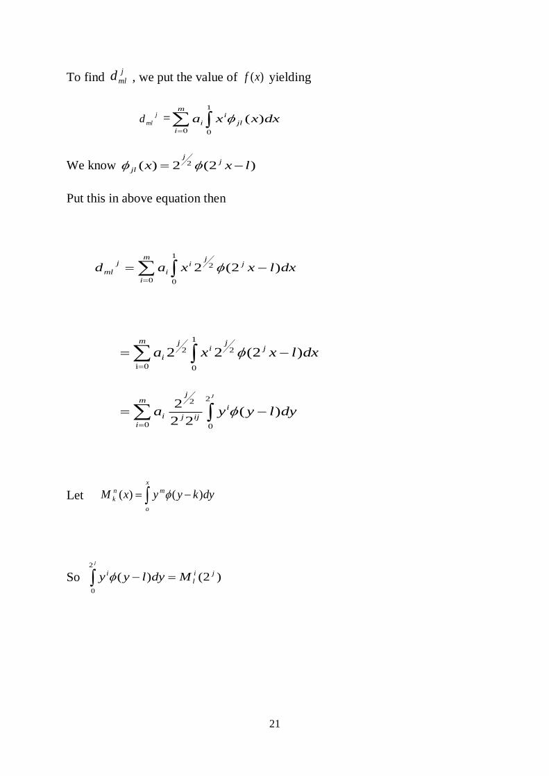
21
To find j
mld , we put the value of )(xf yielding
j
mld =
1
00
)( dxxxa jl
im
i
i
We know )2(2)( 2 lxx jj
jl
Put this in above equation then
)2(20
1
0
2
m
i
jj
i
i
j
ml dxlxxad
1
0
2
0i
2 )2(22 dxlxxa jj
im j
i
m
i
i
ijj
j
i
J
dylyya0
2
0
2
)(22
2
Let
x
o
mn
k dykyyxM )()(
So )2()(
2
0
ji
l
i Mdylyy
j
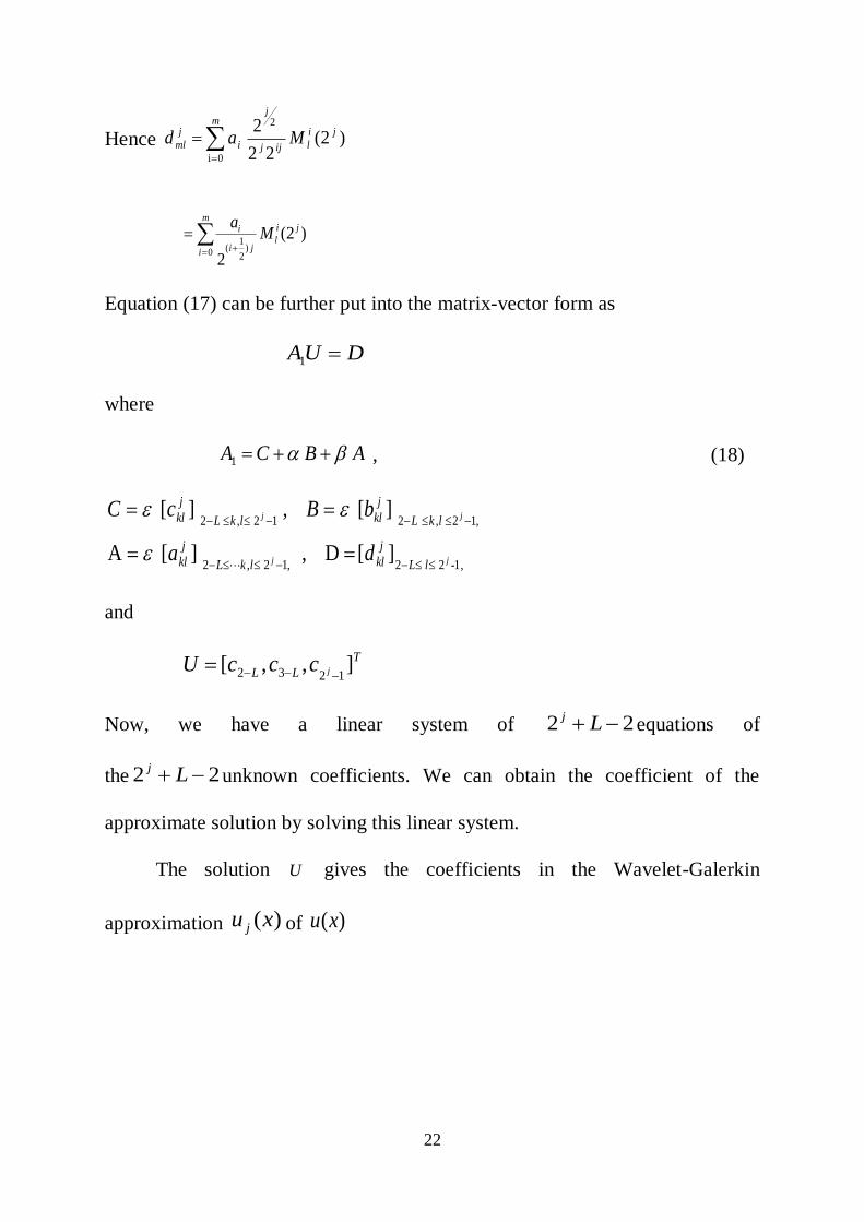
22
Hence )2(22
2
2
0i
ji
lijj
jm
i
j
ml Mad
)2(
2
0 )2
1(
ji
l
m
i ji
i Ma
Equation (17) can be further put into the matrix-vector form as
DUA 1
where
ABCA 1 , (18)
][ D , ][ A
][ , ][
1,-22 ,12,2
,12,212,2
jj
jj
lL
j
kllkL
j
kl
lkL
j
kllkL
j
kl
da
bBcC
and
T
LL jcccU ],,[1232
Now, we have a linear system of 22 Ljequations of
the 22 Ljunknown coefficients. We can obtain the coefficient of the
approximate solution by solving this linear system.
The solution U gives the coefficients in the Wavelet-Galerkin
approximation )(xu j of )(xu

23
CHAPTER-6
Wavelet-Galerkin Solution of Shear Wave Equation:
Consider a plate of finite extent in the z & y direction & of thickness 1 in x
direction. For horizontal polarized shear wave, the governing partial differential
equation is
1
2
2
2 t
u
cuu yyxx
(19)
where ),,( tyxuu
We consider the solution of the wave equation as
.
)(),,( tyietyxu (20)
substitute (20) in (19) we get
0)()( 2
2
2
xudx
xud (21)
where 2
2
22
c
So exact solution is
)(
21 )cossin(),,( tyiexAxAtyxu (22)
Wavelet Galerkin method solution

24
Here, we shall consider 0&6 JL
Consider the solution of ordinary differential equation (21) is
)2(2)(2
1
2 kxcxu j
Lk
j
k
j
, ]1,0[x
1
5
)(k
k kxc , ]1,0[x (23)
Where are constants, the unknown co-efficient
Substitute (23) in (21) we get
0)()(1
5
21
52
2
k
k
k
k kxckxcdx
d
0)()(1
5
21
5
k
k
k
k kxckxc
Without any loss of generality, let 12 and taking inner product with )( nx ,
we have
0)()()()(1
5
2
21
2
1
21
5
2
21
2
1
k
L
L
k
k
L
L
k
j
j
j
j
j
j
nxkxcnxkxc
25
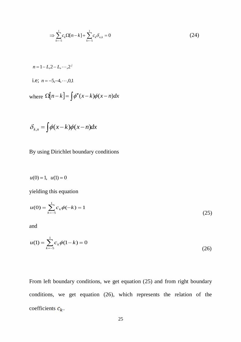
0 ][ ,
1
5
1
5
kn
k
k
k
k cknc (24)
jLLn 2,,2,1
i.e; 1,0,,4,5 n
where dxnxkxkn )()(
dxnxkxnk )()(,
By using Dirichlet boundary conditions
0)1( ,1)0( uu
yielding this equation
1)()0(1
5
k
k kcu (25)
and
0)1()1(1
5
k
k kcu (26)
From left boundary conditions, we get equation (25) and from right boundary
conditions, we get equation (26), which represents the relation of the
coefficients .

26
Now we eliminate first and last equations of (24) and in that places are
including equation (25) and (26) respectively, we get the following matrix
with 6L .
BTC
0)1()2()3()4(00
]1[1]0[]1[]2[]3[]4[]5[
]2[]1[1]0[]1[]2[]3[]4[
]3[]2[]1[1]0[]1[]2[]3[
]4[]3[]2[]1[1]0[]1[]2[
]5[]4[]3[]2[]1[1]0[]1[
00)1()2()3()4(0
T
1
0
1
2
3
4
5
c
c
c
c
c
c
c
C and
0
0
0
0
0
0
1
B
By Gaussian elimination algorithm we get
997181.05 c
877618.03 c
127868.02 c

27
08705.11 c
24756.00 c
505899.01 c
The Exact solution by using Dirichlet boundary condition is
xxxu sin1cotcos)(
Table-4 shows the comparison between Wavelet-Galerkin solution and Exact
solution
Table 4 Comparison between wavelet Solution and Exact Solution
x Wavelet solution Exact solution Absolute Error
0 1 1 0
0.125 0.921657 0.912145 0.00951209
0.25 0.829106 0.810056 .0190502
0.375 0.726413 0.69535 0.031086
0.5 0.609339 0.569747 0.0395922
0.625 0.477075 0.435276 0.041798
0.75 0.331501 0.294014 0.0374878
0.875 0.172689 0.148163 0.0245264
1 0 0 0
The value of above table & using MATLAB we obtain the following graph

28
Figure 2: Comparison between wavelet Solution and Exact Solution
.To exhibit a comparison between Wavelet-Galerkin solution and Exact
solution, figure2 has been diagrammed by MATLAB. A good agreement of
result has been obtained as doted by figure 2.

29
CHAPTER-7
CONCLUSION
Wavelet-Galerkin method is the most frequenly used scheme now a days.
In the present project work, the Daubechies family of the wavelet have been
consider. Due to the fact that they posses several useful properties, such as
orthogonality, compact support, exact representation of polynomials to a certain
degree and ability to represent function at different levels resolution.
Dabauchies’ wavelets have gained great interest in the numerical solution of
ordinary and partial differential equation.
An obtain advantages of this method of this method is that it uses Daubechies’
coefficients and calculate the Scaling function, the connection coefficients as
well as the rest of component only once.
This leads to a considerable saving of the computational time and improves
numerical results through the reduction of round-off errors.
The Wavelet-Galerkin method has been shown to be a powerful numerical tool
for fast and more accurate solution of differential equations, it can be observed
from the result. Wavelet Galerkin method yields better result, which shows the
effiency of the method.
30
Solution obtained using the Daubechies 6 coefficients wavelet has been
compared with the exact solution. The good agreement of its numerical result
with the exact solution proves its accuracy and efficiency .

31
BIBLIOGRAPHY
[1] Daubechis,I, 1992 , Ten Lectures on Wavelet, Capital City Press, Vermont.
[2] qian,s. and Weiss,J.,1993 Wavelet and the numerical solution of boundary
value problem, Appl. Math. Lett, 6, 47-52
[3] qian,s., and Weiss,J.,1993 Wavelet and the numerical solution of partial
differential equation ‘, J. Comput. Phys, 106, 155-175
[4] Williams,J.R.and Amaratunga,K., 1992, Intriduction to Wavelet in
engineering, IESL Tech.Rep.No.92-07,Intelegent Engineering system
labrotary,MIT.
[5] Daubechies,I.,1988, Orthonormal bases of compactly supported wavelets,
Commun. Pure Appl. Math., 41, 909-996.
[6] Beylkin,G., coifman,R. and Rokhlin,V., 1991,Fast Wavelet Transfermation
and Numerical Algorithm, Comm. Pure Applied Math.,44,141-183
[7] K. Amaratunga, J.R. William, s. qian and J. Weiss, wavelet-Galerkin
solution for one dimentional partial differential equations, Int. J. numerical
methods eng. 37, 2703-2716 (1994).
[8] Latto,A., Resnikoff, H.L and Tenenbaum,E., 1992 The Evaluation of
connection coefficients of compactly Supported Wavelet: in proceedings of the
French-USA Workshop on Wavelet and Turbulence, Princeton, New York, June
1991,Springer- Verlag,.

32
[9] Williams,J.R.and Amaratunga,K.,1994, High order Wavelet extrapolation
schemes for initial problem and boundary value problem,IESL Tech.Rep.No.94-
07,Inteligent Engineering systems Labrotary,MIT.
[10] J.c., and W.-c., Galerkin-Wavelet method for two point boundary value
problems, Number. Math.63 (1992) 123-144.
[11] Comparison of boundary by Adomain decomposition and Wavelet-
Galerkin methods of boundary-value problem,181(2007)652-664
[12]The computation of Wavelet-Galerkin method on a bounded interval,
International Journal for Numerical Methods in Engineering,Vol.39,2921-2944
[13] Treatment of Boundary Conditions in the Application of Wavelet-Galerkin
Method to a SH Wave Problem. Dianfeng LU, Tadashi OHYOSHI,Lin ZHU.
[14] Wavelet-Galerkin solution of ordinary differential equations, Vinod Mishra
and Sabina, Int. Journal of Math. Analysis, Vol.5, 2011, no.407-424
[15] S.Mallat, Multiresolution approximation and wavelets, Trans. Amer. Math.
Soc., 315,69-88(1989).

33

34

35