NASA Contractor Report 4675

A Verification Procedure for MSC/NASTRAN FiniteElement Models

Alan E. StockwellLockheed Engineering & Sciences Company, Hampton, Virginia

Prepared for Langley Research CenterUnder Contract NAS1-19000

May 1995

i

Acknowledgments

The author wishes to acknowledge the contributions of Mercedes Reaves and RaymondKvaternik of NASA Langley Research Center. Both Ray and Mercedes offered severalhelpful suggestions, and Ray supplied a stack of related publications from his personalfiles.

ii

Table of Contents

Acknowledgements i

1.0 Introduction 1

2.0 Preprocessor Checks 1

3.0 Analytical Checks 2

4.0 Model Verification Procedure 9

5.0 Summary 17

6.0 References 18

1

1.0 Introduction

Finite element models (FEMs) are used in the design and analysis of aircraft tomathematically describe the airframe structure for such diverse tasks as flutter analysis andactively controlled landing gear design. FEMs are used to model the entire airplane as wellas airframe components. Model verification procedures are especially important for large-scale FEMs of an entire airplane which are developed by an outside contractor or agencyand are used for aeroelastic and dynamic analyses. Since there is no test data to validatethe FEMs during the preliminary design stage, it is especially important for both modeldevelopers and users to understand the limitations of the models and to ensure that theyare used correctly. The purpose of this document is to describe recommended methods forverifying the quality of the FEMs and to specify a step-by-step procedure for implementingthe methods. The procedure has been successfully applied to large-scale FEMs ofpreliminary design concepts for the NASA High Speed Civil Transport (HSCT) aircraft.

The document is divided into four sections. Section 1 is the Introduction. Section 2,Preprocessor Checks, briefly describes suggested procedures for checking a model using agraphical preprocessor. Section 3, Analytical Checks, describes methods of verifying themathematical correctness of the model using the MSC/NASTRAN finite element code.Section 4, Model Verification Procedure, presents a step-by-step procedure forimplementing the analytical checks described in Section 3. Section 4 is intended to be aworking document containing a "cookbook" procedure to facilitate the model checkingprocess and help ensure a consistent level of quality. Although this procedure mayuncover modeling errors, it is not an exhaustive investigation of modeling details, nor doesit address the issue of whether the structure is modeled appropriately. The assumption ismade that the structure was carefully modeled by the developer. The FEM user's task is toensure only that the model makes mathematical sense and contains no obvious errors oromissions.

Several methods, such as kinetic energy and effective mass, can be used to evaluate thedynamic properties of FEMs. These methods can also identify weaknesses or modelingerrors. However, their primary purposes are to characterize the dynamics of the structureand to guide a dynamicist in selecting a valid set of structural vibration modes for aparticular analysis. A discussion of these methods is beyond the scope of this document.

2.0 Preprocessor Checks

2.1 Introduction

Preprocessor model checks are important in developing a FEM. However, some of thestandard checks employed in the model development process (e.g., element aspect ratio ortaper) may not be necessary or appropriate when a model created by another organizationis being verified. The discussion that follows focuses on those particular preprocessorchecks which are valuable tools in verifying a model developed outside the user'sorganization.

2

2.2 Visual Checks

An analyst using a FEM developed by an outside source can employ preprocessor visualchecks to become familiar with the model and to ensure that it looks reasonable.Preprocessor plots of the model allow the analyst to verify the overall shape of the model,as well as key dimensions. If more than one coordinate system has been used to definemodel geometry, the plots are an excellent method of determining whether key structuraldetails are oriented correctly. Most preprocessors allow the user to group grid points andelements according to criteria such as physical or material property number. Although itmay not be feasible to check every property in a model, the plots offer a quick method ofchecking selected data. Plots of loads and boundary conditions can also be used to quicklycheck that they are applied correctly.

It should be recognized that every time a translation is made from one analysis orpreprocessor code to another (e.g., PATRAN [1] to NASTRAN [2], NASTRAN to I-DEAS[3], etc.), there is a potential for introducing errors. The analytical checks described inSection 3 provide a good basis for ensuring that the results of some of the preprocessorchecks are still valid after the model has been translated into an MSC/NASTRAN input file.

2.3 Element Checks

Most preprocessors will perform element distortion checks that measure quantities such astaper, skew angle and aspect ratios. Modeling details that violate generally acceptedguidelines may not necessarily be incorrect. However, it is useful for an analyst to beaware of the expected quality of results obtained from various parts of the model.

Weight property checks may also be useful. Differences in the results between the analysisprogram and the preprocessor may indicate translation problems.

2.4 Summary

This section has presented some brief guidelines for using a graphical preprocessor toverify a model. A detailed discussion of commercial FEM preprocessors is beyond thescope of this document, and it is left to the individual analyst to correctly use the features ofa selected preprocessor in an effective manner.

3.0 Analytical Checks

3.1 Introduction

The purpose of the analytical checks described in this section is to ensure the mathematicalsoundness of the model and to uncover any gross modeling errors, such as missingelements or incorrectly applied boundary conditions. The material presented hereinconsists of generally accepted practices and procedures. Most of the methods aredescribed in references 4, 5 and 6.

3

3.2 Pre-analysis Mass, Stiffness and Matrix Reduction Checks

Several analytical model checks can be performed prior to any static or dynamic analysis.These checks are referred to as "pre-analysis" checks, because they are computationswhich are performed on the mass and/or stiffness matrices and are independent of specificboundary conditions or applied loads.

3.2.1 Constraint Checking

MSC/NASTRAN [2 ] provides the option in any of the Structured Solution sequences (SOL101-200) of requesting a "superelement checkout" run by including"PARAM,CHECKOUT,YES" in either the Bulk Data Deck or Case Control Deck. The"checkout" option triggers a series of checks in the "Bookkeeping and Control" (Phase 0)subDMAP. The run is automatically terminated before the matrix assembly, generation andreduction operations begin in the Phase I subDMAP. While this option is primarily intendedfor checking superelement models, it includes a sequence of multipoint constraint checkswhich are useful for any model. These checks detect the presence of internal constraints(grounding) and ill-conditioning. The checks operate on the multipoint constraint equationmatrix, Rmg, formed in module GP4 from the MPC and rigid body Bulk Data entries. Inorder to perform the checks, NASTRAN partitions Rmg into dependent (m-set) andindependent (n-set) sub-matrices, i.e., Rmg = Rmm Rmn . As described in Section 9.4.1 ofreference 2, three tests are performed:

1. A matrix of rigid-body vectors, ugho , is assembled using the VECPLOT module, and the

product

Emh = Rmgugho

is calculated. The terms of Emh larger than PARAM,TINY are printed. These terms usuallyindicate internal constraints, although exceptions to this may occur if there are MPCequations involving scalar points. A simple example of an internal constraint is an MPCequation involving two degrees of freedom, in which the coefficient for the independentdegree of freedom is inadvertently left blank. NASTRAN will assume that the coefficient iszero, thereby grounding the dependent degree of freedom.

2. The product Rmmg = RmgRmg

T is calculated and decomposed by the DCMP module.During the solution process, NASTRAN decomposes symmetric structural matrices intoupper and lower triangular factors and a diagonal matrix, e.g.,

K = L D LT

where L is the lower triangular factor and D is called the "factor diagonal matrix." Note thatthe upper triangular factor for a symmetric matrix is equal to LT. Symmetric decomposition,followed by forward/backward substitution, is a computationally efficient alternative tomatrix inversion. An additional benefit of decomposition in MSC/NASTRAN is thediagnostic messages that alert the user to problems in the matrices. Each diagonal term ofK is divided by the corresponding term of the factor diagonal matrix, D, and ratios largerthan PARAM,MAXRATIO are printed. The number and location of any negative terms in

4

the factor diagonal matrix are also printed. In the case of the constraint matrix, Rmg, theterms flagged by the decomposition of Rmm

g indicate the presence of linearly dependentrows in Rmg, i.e., redundant constraints. This condition will probably cause singularities orpoorly conditioned constraints if the problem is not corrected.

3. The product Rmmm = RmmRmm

T is calculated and decomposed, and factor diagonal termslarger than MAXRATIO are printed. The results of this check may be compared to theresults of step 2. A degree of freedom flagged here that was not flagged in step 2 indicatesthat a problem exists in the dependent partition, Rmm, but not in the matrix containing allDOF (Rmg ). Therefore, an error was made in specifying the dependent degrees offreedom.

The "checkout" option automatically stops the solution process after the constraint checks.Additional model verification may be accomplished by using either specially-developedDirect Matrix Abstraction Programs (DMAPs) or static analyses.

3.2.2 Grid Point Weight Generator (GPWG)

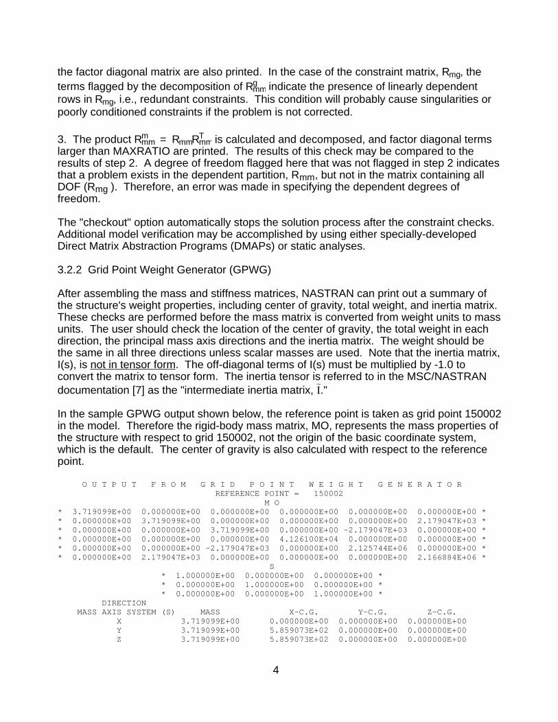
After assembling the mass and stiffness matrices, NASTRAN can print out a summary ofthe structure's weight properties, including center of gravity, total weight, and inertia matrix.These checks are performed before the mass matrix is converted from weight units to massunits. The user should check the location of the center of gravity, the total weight in eachdirection, the principal mass axis directions and the inertia matrix. The weight should bethe same in all three directions unless scalar masses are used. Note that the inertia matrix,I(s), is not in tensor form. The off-diagonal terms of I(s) must be multiplied by -1.0 toconvert the matrix to tensor form. The inertia tensor is referred to in the MSC/NASTRANdocumentation [7] as the "intermediate inertia matrix, I."

In the sample GPWG output shown below, the reference point is taken as grid point 150002in the model. Therefore the rigid-body mass matrix, MO, represents the mass properties ofthe structure with respect to grid 150002, not the origin of the basic coordinate system,which is the default. The center of gravity is also calculated with respect to the referencepoint.

O U T P U T F R O M G R I D P O I N T W E I G H T G E N E R A T O R REFERENCE POINT = 150002 M O* 3.719099E+00 0.000000E+00 0.000000E+00 0.000000E+00 0.000000E+00 0.000000E+00 ** 0.000000E+00 3.719099E+00 0.000000E+00 0.000000E+00 0.000000E+00 2.179047E+03 ** 0.000000E+00 0.000000E+00 3.719099E+00 0.000000E+00 -2.179047E+03 0.000000E+00 ** 0.000000E+00 0.000000E+00 0.000000E+00 4.126100E+04 0.000000E+00 0.000000E+00 ** 0.000000E+00 0.000000E+00 -2.179047E+03 0.000000E+00 2.125744E+06 0.000000E+00 ** 0.000000E+00 2.179047E+03 0.000000E+00 0.000000E+00 0.000000E+00 2.166884E+06 * S * 1.000000E+00 0.000000E+00 0.000000E+00 * * 0.000000E+00 1.000000E+00 0.000000E+00 * * 0.000000E+00 0.000000E+00 1.000000E+00 * DIRECTION MASS AXIS SYSTEM (S) MASS X-C.G. Y-C.G. Z-C.G. X 3.719099E+00 0.000000E+00 0.000000E+00 0.000000E+00 Y 3.719099E+00 5.859073E+02 0.000000E+00 0.000000E+00 Z 3.719099E+00 5.859073E+02 0.000000E+00 0.000000E+00

5

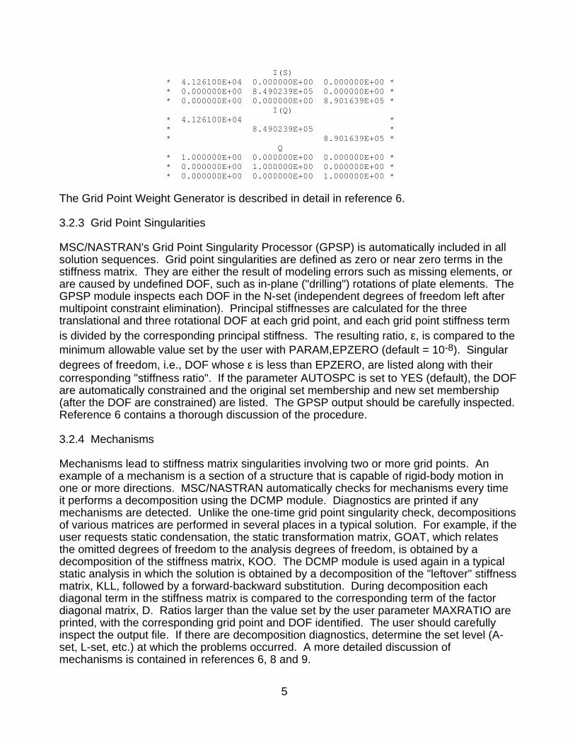
I(S) * 4.126100E+04 0.000000E+00 0.000000E+00 * * 0.000000E+00 8.490239E+05 0.000000E+00 * * 0.000000E+00 0.000000E+00 8.901639E+05 * I(Q) * 4.126100E+04 * * 8.490239E+05 * * 8.901639E+05 * Q * 1.000000E+00 0.000000E+00 0.000000E+00 * * 0.000000E+00 1.000000E+00 0.000000E+00 * * 0.000000E+00 0.000000E+00 1.000000E+00 *

The Grid Point Weight Generator is described in detail in reference 6.

3.2.3 Grid Point Singularities

MSC/NASTRAN's Grid Point Singularity Processor (GPSP) is automatically included in allsolution sequences. Grid point singularities are defined as zero or near zero terms in thestiffness matrix. They are either the result of modeling errors such as missing elements, orare caused by undefined DOF, such as in-plane ("drilling") rotations of plate elements. TheGPSP module inspects each DOF in the N-set (independent degrees of freedom left aftermultipoint constraint elimination). Principal stiffnesses are calculated for the threetranslational and three rotational DOF at each grid point, and each grid point stiffness termis divided by the corresponding principal stiffness. The resulting ratio, ε, is compared to theminimum allowable value set by the user with PARAM,EPZERO (default = 10-8). Singulardegrees of freedom, i.e., DOF whose ε is less than EPZERO, are listed along with theircorresponding "stiffness ratio". If the parameter AUTOSPC is set to YES (default), the DOFare automatically constrained and the original set membership and new set membership(after the DOF are constrained) are listed. The GPSP output should be carefully inspected.Reference 6 contains a thorough discussion of the procedure.

3.2.4 Mechanisms

Mechanisms lead to stiffness matrix singularities involving two or more grid points. Anexample of a mechanism is a section of a structure that is capable of rigid-body motion inone or more directions. MSC/NASTRAN automatically checks for mechanisms every timeit performs a decomposition using the DCMP module. Diagnostics are printed if anymechanisms are detected. Unlike the one-time grid point singularity check, decompositionsof various matrices are performed in several places in a typical solution. For example, if theuser requests static condensation, the static transformation matrix, GOAT, which relatesthe omitted degrees of freedom to the analysis degrees of freedom, is obtained by adecomposition of the stiffness matrix, KOO. The DCMP module is used again in a typicalstatic analysis in which the solution is obtained by a decomposition of the "leftover" stiffnessmatrix, KLL, followed by a forward-backward substitution. During decomposition eachdiagonal term in the stiffness matrix is compared to the corresponding term of the factordiagonal matrix, D. Ratios larger than the value set by the user parameter MAXRATIO areprinted, with the corresponding grid point and DOF identified. The user should carefullyinspect the output file. If there are decomposition diagnostics, determine the set level (A-set, L-set, etc.) at which the problems occurred. A more detailed discussion ofmechanisms is contained in references 6, 8 and 9.

6

3.2.5 Multi-Level Strain Energy Checks

Multi-level strain energy checks are another means of detecting modeling errors. Thechecks are not built into the structured solution sequences, however a DMAP alter isavailable. The alter, "checka.v68", is located in the "misc" subdirectory on theMSC/NASTRAN delivery tape. The checks are referred to as "multi-level" because thecomputations are performed at various set levels such as the G-set, N-set, and A-set level.Since each level represents a significant step in the reduction process leading to the finalequations, the checks can be a useful means of determining both the location and thecause of errors. For example, an error that occurs at the A-set level, but does not occur atthe N-set level, would be caused by a static or dynamic reduction error rather than a rigid-body constraint problem.

An important issue to consider when using these checks is the application of specificboundary conditions. If all single point constraints except those that involve zero-stiffnessDOF (e.g., drilling rotations in QUAD4 plate elements) are removed, then the checks will beindependent of specific boundary conditions. This may be useful in identifying hiddenproblems, such as grounding. However, the analyst may also want to check the effects ofthe single point constraint (SPC) elimination (See the discussion in section 3.2).

The multi-level strain energy check procedure consists of computing a set of six rigid-bodydisplacement vectors, then using them to compute forces, rigid-body strain energy, andrigid-body mass matrices. The checks proceed as follows:

Stiffness Checks:

1. At the G-set level, compute a set of rigid-body vectors, RBG, using the VECPLOTmodule.

2. Compute the reaction forces resulting from the rigid-body motion, and print thenormalized non-zero forces:

REACG = KGG * RBG

3. Compute and print the strain energy:

CHKKGG = RBGT * REACG

4. Repeat steps 1 through 3 at the N-set level (the N set contains all independent DOF noteliminated by multipoint constraints).

5. Repeat steps 1 through 3 at the A-set level. To obtain the A-set stiffness matrix,NASTRAN first partitions the N set into the F set (free DOF) and the S set (DOF eliminatedby single point constraints). The F set is then partitioned into A set (analysis set) and O set(omitted) DOF, and a reduced stiffness matrix, KAA, is typically computed by the process ofGuyan (static) reduction, generalized dynamic reduction, or component mode synthesis. Ifno reduction is requested by the user, the F set and A set will be equivalent.

7

The diagonal terms of the strain energy matrix should all be nearly zero if there are noerrors (such as grounding problems) in the stiffness matrix. The reaction forces arenormalized by dividing each term by the largest term in the vector. If there are non-zeroterms, the elements of the normalized reaction force matrix (REACGNRM, REACNNRM, orREACANRM) can be surveyed to find the largest forces.

Mass Checks:

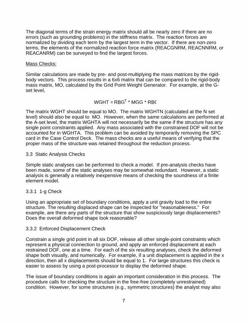
Similar calculations are made by pre- and post-multiplying the mass matrices by the rigid-body vectors. This process results in a 6x6 matrix that can be compared to the rigid-bodymass matrix, MO, calculated by the Grid Point Weight Generator. For example, at the G-set level,

WGHT = RBGT * MGG * RBG

The matrix WGHT should be equal to MO. The matrix WGHTN (calculated at the N setlevel) should also be equal to MO. However, when the same calculations are performed atthe A-set level, the matrix WGHTA will not necessarily be the same if the structure has anysingle point constraints applied. Any mass associated with the constrained DOF will not beaccounted for in WGHTA. This problem can be avoided by temporarily removing the SPCcard in the Case Control Deck. The mass checks are a useful means of verifying that theproper mass of the structure was retained throughout the reduction process.

3.3 Static Analysis Checks

Simple static analyses can be performed to check a model. If pre-analysis checks havebeen made, some of the static analyses may be somewhat redundant. However, a staticanalysis is generally a relatively inexpensive means of checking the soundness of a finiteelement model.

3.3.1 1-g Check

Using an appropriate set of boundary conditions, apply a unit gravity load to the entirestructure. The resulting displaced shape can be inspected for "reasonableness." Forexample, are there any parts of the structure that show suspiciously large displacements?Does the overall deformed shape look reasonable?

3.3.2 Enforced Displacement Check

Constrain a single grid point in all six DOF, release all other single-point constraints whichrepresent a physical connection to ground, and apply an enforced displacement at eachrestrained DOF, one at a time. For each of the six resulting analyses, check the deformedshape both visually, and numerically. For example, if a unit displacement is applied in the xdirection, then all x displacements should be equal to 1. For large structures this check iseasier to assess by using a post-processor to display the deformed shape.

The issue of boundary conditions is again an important consideration in this process. Theprocedure calls for checking the structure in the free-free (completely unrestrained)condition. However, for some structures (e.g., symmetric structures) the analyst may also

8

want to check the structure with SPCs applied to insure that strain-free motion is stillpossible in the DOF that are not affected by the boundary restraints.

3.3.3 Checks Against Reference Data

Frequently there exists analytical or experimental data which can be used to validate themodel. For example, if a model is delivered from one contractor to another, then translatedfrom one analysis program to another, the results of the translation can be checked if a setof reference data is available. This might take the form of a set of displacements orelement forces caused by a given loading. It is a relatively simple task to make such acomparison. Test data, if available, can also be used to check a model. However, sincetest/analysis correlation is not an exact science, care should be taken in interpreting theresults.

3.4 Checking Static Analysis Output

After a static analysis has been executed, NASTRAN provides several diagnostics that canbe used to check the results. The output is described briefly in the following sections.Reference 6 contains a detailed description of these features.

3.4.1 FBS Diagnostics

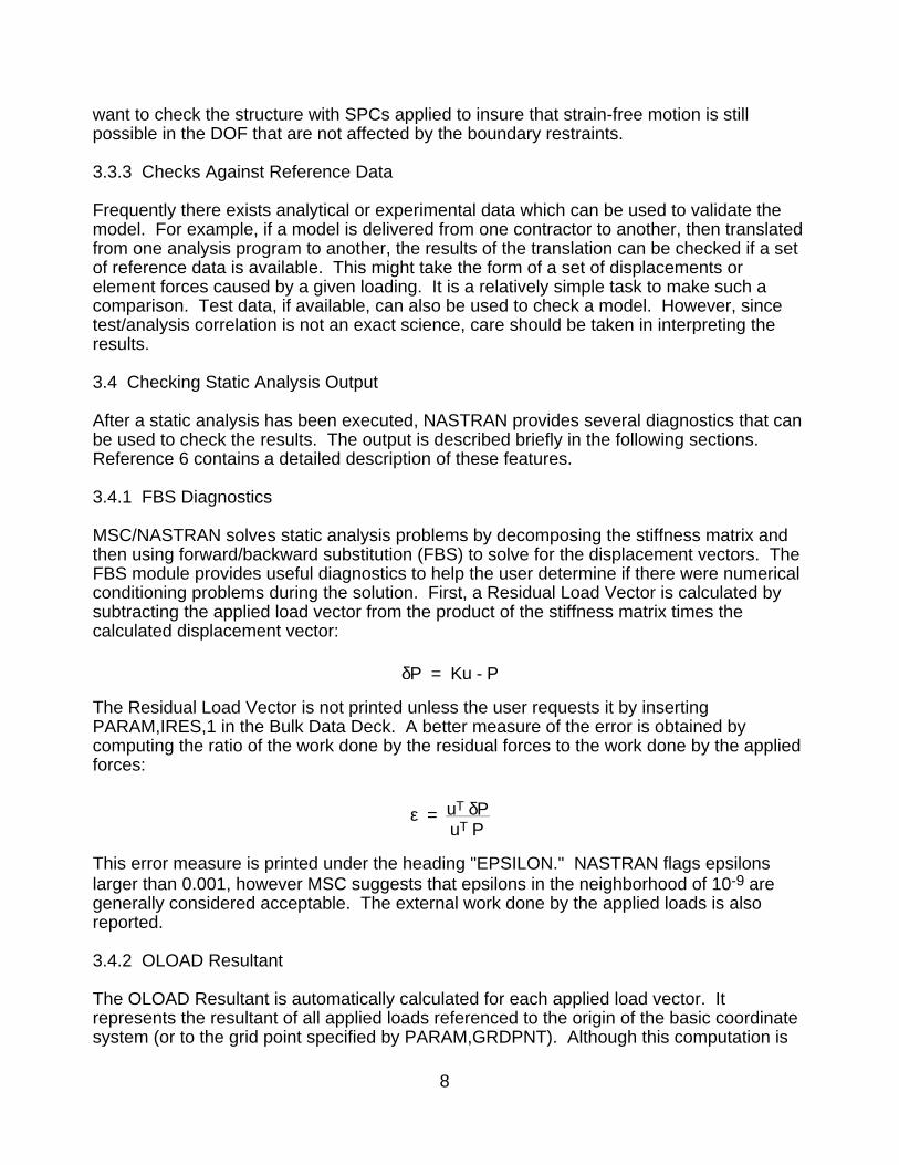
MSC/NASTRAN solves static analysis problems by decomposing the stiffness matrix andthen using forward/backward substitution (FBS) to solve for the displacement vectors. TheFBS module provides useful diagnostics to help the user determine if there were numericalconditioning problems during the solution. First, a Residual Load Vector is calculated bysubtracting the applied load vector from the product of the stiffness matrix times thecalculated displacement vector:

δP = Ku - P

The Residual Load Vector is not printed unless the user requests it by insertingPARAM,IRES,1 in the Bulk Data Deck. A better measure of the error is obtained bycomputing the ratio of the work done by the residual forces to the work done by the appliedforces:

ε = uT δP

uT P

This error measure is printed under the heading "EPSILON." NASTRAN flags epsilonslarger than 0.001, however MSC suggests that epsilons in the neighborhood of 10-9 aregenerally considered acceptable. The external work done by the applied loads is alsoreported.

3.4.2 OLOAD Resultant

The OLOAD Resultant is automatically calculated for each applied load vector. Itrepresents the resultant of all applied loads referenced to the origin of the basic coordinatesystem (or to the grid point specified by PARAM,GRDPNT). Although this computation is

9

an applied loads check, and is not really a model check, it is an important considerationwhen static loads are being used to check out a model. OLOAD output at the grid pointlevel can be requested by using the Case Control OLOAD card.

3.4.3 SPCFORCE Resultant

The SPCFORCE Resultant is the summation of all forces of single point constraint withrespect to the reference point. As in the OLOAD summation, the reference point is eitherthe grid point specified by PARAM,GRDPNT, or the origin of the basic coordinate system.SPCFORCES can also be printed for individual grid points. A useful equilibrium check canbe made by summing the SPCFORCE Resultant and the OLOAD Resultant.

3.4.4 Maximum Load

NASTRAN automatically prints a summary of the maximum load in each direction (of thebasic coordinate system) for each load vector. Care must be taken when reading thisoutput. The maximum load may not occur at the same grid point for any of the sixdirections, and the table gives no information as to where the maximum loads occurred.This information can be useful as a "sanity" check.

3.4.5 Maximum Displacement

The table of maximum displacements is also printed for each of the six basic coordinatedirections for each load vector. No location information is given, however the table isanother useful means of checking that the magnitudes of the displacements make sensefor each direction.

4.0 Model Verification Procedure

4.1 Introduction

The model verification procedure described in this section is based on the techniquesoutlined in the previous sections. The procedures have been used for checking a non-superelement High Speed Civil Transport (HSCT) model generated outside of LaRC,delivered in a foreign FE code format and translated into MSC/NASTRAN format. Asdescribed in Section 1, the procedures are intended primarily to verify that the model ismathematically correct. Modeling issues such as mesh density, element type and usage,and connection details are difficult to check in an objective sense, and are beyond thescope of this document. It is assumed in this section that the model has already beentranslated into MSC/NASTRAN form and has been checked with a graphical preprocessor.See the discussion on analytical checks in Section 3 for more detailed descriptions of theMSC/NASTRAN procedures and calculations.

4.2 Constraint Checks

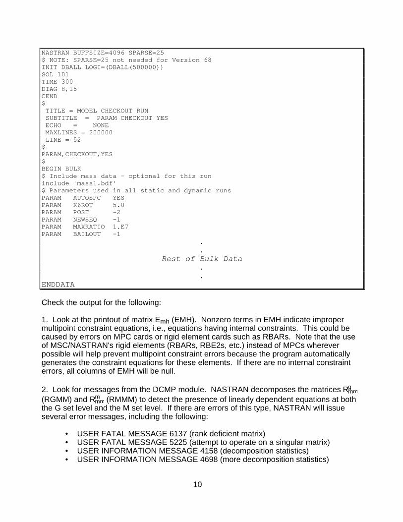
Set up a static analysis run (SOL 101), and include "PARAM,CHECKOUT,YES" in theCase Control or Bulk Data deck. A sample deck is shown below.

10

NASTRAN BUFFSIZE=4096 SPARSE=25$ NOTE: SPARSE=25 not needed for Version 68INIT DBALL LOGI=(DBALL(500000))SOL 101TIME 300DIAG 8,15CEND$ TITLE = MODEL CHECKOUT RUN SUBTITLE = PARAM CHECKOUT YES ECHO = NONE MAXLINES = 200000 LINE = 52$PARAM,CHECKOUT,YES$BEGIN BULK$ Include mass data - optional for this runinclude 'mass1.bdf'$ Parameters used in all static and dynamic runsPARAM AUTOSPC YESPARAM K6ROT 5.0PARAM POST -2PARAM NEWSEQ -1PARAM MAXRATIO 1.E7PARAM BAILOUT -1

.

.Rest of Bulk Data

.

.ENDDATA

Check the output for the following:

1. Look at the printout of matrix Emh (EMH). Nonzero terms in EMH indicate impropermultipoint constraint equations, i.e., equations having internal constraints. This could becaused by errors on MPC cards or rigid element cards such as RBARs. Note that the useof MSC/NASTRAN's rigid elements (RBARs, RBE2s, etc.) instead of MPCs whereverpossible will help prevent multipoint constraint errors because the program automaticallygenerates the constraint equations for these elements. If there are no internal constrainterrors, all columns of EMH will be null.

2. Look for messages from the DCMP module. NASTRAN decomposes the matrices Rmmg

(RGMM) and Rmmm (RMMM) to detect the presence of linearly dependent equations at both

the G set level and the M set level. If there are errors of this type, NASTRAN will issueseveral error messages, including the following:

• USER FATAL MESSAGE 6137 (rank deficient matrix)• USER FATAL MESSAGE 5225 (attempt to operate on a singular matrix)• USER INFORMATION MESSAGE 4158 (decomposition statistics)• USER INFORMATION MESSAGE 4698 (more decomposition statistics)

11

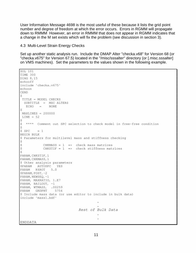
User Information Message 4698 is the most useful of these because it lists the grid pointnumber and degree of freedom at which the error occurs. Errors in RGMM will propagatedown to RMMM However, an error in RMMM that does not appear in RGMM indicates thata change in the M set exists which will fix the problem (see discussion in section 3).

4.3 Multi-Level Strain Energy Checks

Set up another static analysis run. Include the DMAP Alter "checka.v68" for Version 68 (or"checka.v675" for Version 67.5) located in the "/misc/sssalter" directory (or [.misc.sssalter]on VMS machines). Set the parameters to the values shown in the following example.

SOL 101TIME 300DIAG 8,15echooffinclude 'checka.v675'echoonCEND$ TITLE = MODEL CHECKS SUBTITLE = MSC ALTERS ECHO = NONE$ MAXLINES = 200000 LINE = 52$$ **** Comment out SPC selection to check model in free-free condition$$ SPC = 1BEGIN BULK$ Parameters for multilevel mass and stiffness checking$$ CHKMASS = 1 => check mass matrices$ CHKSTIF = 1 => check stiffness matrices$PARAM,CHKSTIF,1PARAM,CHKMASS,1$ Other analysis parameters$PARAM AUTOSPC YESPARAM K6ROT 5.0$PARAM,POST,-2PARAM,NEWSEQ,-1PARAM, MAXRATIO, 1.E7PARAM, BAILOUT, -1PARAM, WTMASS, .00259PARAM GRDPNT 5754$ Include mass data (or use editor to include in bulk data)include 'mass1.bdf'

.

.Rest of Bulk Data

.

.ENDDATA

12

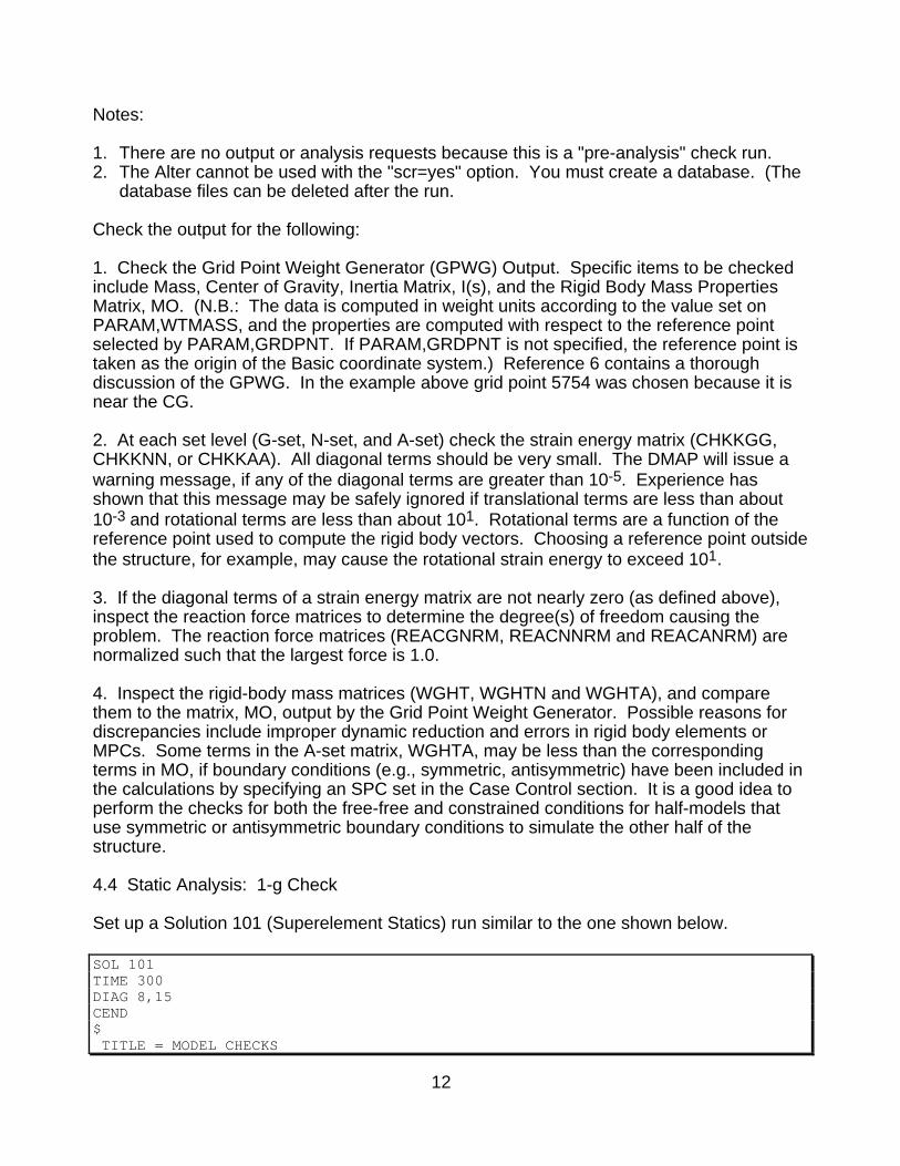
Notes:

1. There are no output or analysis requests because this is a "pre-analysis" check run.2. The Alter cannot be used with the "scr=yes" option. You must create a database. (The

database files can be deleted after the run.

Check the output for the following:

1. Check the Grid Point Weight Generator (GPWG) Output. Specific items to be checkedinclude Mass, Center of Gravity, Inertia Matrix, I(s), and the Rigid Body Mass PropertiesMatrix, MO. (N.B.: The data is computed in weight units according to the value set onPARAM,WTMASS, and the properties are computed with respect to the reference pointselected by PARAM,GRDPNT. If PARAM,GRDPNT is not specified, the reference point istaken as the origin of the Basic coordinate system.) Reference 6 contains a thoroughdiscussion of the GPWG. In the example above grid point 5754 was chosen because it isnear the CG.

2. At each set level (G-set, N-set, and A-set) check the strain energy matrix (CHKKGG,CHKKNN, or CHKKAA). All diagonal terms should be very small. The DMAP will issue awarning message, if any of the diagonal terms are greater than 10-5. Experience hasshown that this message may be safely ignored if translational terms are less than about10-3 and rotational terms are less than about 101. Rotational terms are a function of thereference point used to compute the rigid body vectors. Choosing a reference point outsidethe structure, for example, may cause the rotational strain energy to exceed 101.

3. If the diagonal terms of a strain energy matrix are not nearly zero (as defined above),inspect the reaction force matrices to determine the degree(s) of freedom causing theproblem. The reaction force matrices (REACGNRM, REACNNRM and REACANRM) arenormalized such that the largest force is 1.0.

4. Inspect the rigid-body mass matrices (WGHT, WGHTN and WGHTA), and comparethem to the matrix, MO, output by the Grid Point Weight Generator. Possible reasons fordiscrepancies include improper dynamic reduction and errors in rigid body elements orMPCs. Some terms in the A-set matrix, WGHTA, may be less than the correspondingterms in MO, if boundary conditions (e.g., symmetric, antisymmetric) have been included inthe calculations by specifying an SPC set in the Case Control section. It is a good idea toperform the checks for both the free-free and constrained conditions for half-models thatuse symmetric or antisymmetric boundary conditions to simulate the other half of thestructure.

4.4 Static Analysis: 1-g Check

Set up a Solution 101 (Superelement Statics) run similar to the one shown below.

SOL 101TIME 300DIAG 8,15CEND$ TITLE = MODEL CHECKS

13

SUBTITLE = 1-G Loads in X, Y, and Z directions ECHO = NONE$$MAXLINES = 200000 LINE = 52$ DISP(plot)=all$$ - - - - - - - - - - - - - - - - - - - - - - - - - - - - - - - - - - - SUBCASE 1 LABEL = Gravity in +X Direction, Symmetric BCs SPC = 1 LOAD = 101 SUBCASE 2 LABEL = Gravity in +Y Direction, Symmetric BCs SPC = 1 LOAD = 102 SUBCASE 3 LABEL = Gravity in +Z Direction, Symmetric BCs SPC = 1 LOAD = 103BEGIN BULKinclude 'mass1.bdf'GRAV 101 0 386.1 1.0 0.0 0.0GRAV 102 0 386.1 0.0 1.0 0.0GRAV 103 0 386.1 0.0 0.0 1.0$PARAM AUTOSPC YESPARAM K6ROT 5.0PARAM POST -2PARAM NEWSEQ -1PARAM MAXRATIO 1.E7PARAM BAILOUT -1PARAM GRDPNT 0PARAM WTMASS .00259..$ Constraints for Static Test Loads$ ---------------------------------$ The following constraints are used to support the model for the$ static load checks. They are used in addition to the free-free$ symmetric constraints. They should be removed before calculating$ symmetric normal modes.$SPC1 1 3 5639SPC1 1 13 5754...ENDDATA

Notes:

1. The gravity loads are applied with symmetric boundary conditions enforced for thesubcases shown (SPC=1). Additional supports (shown in the Bulk Data deck above)

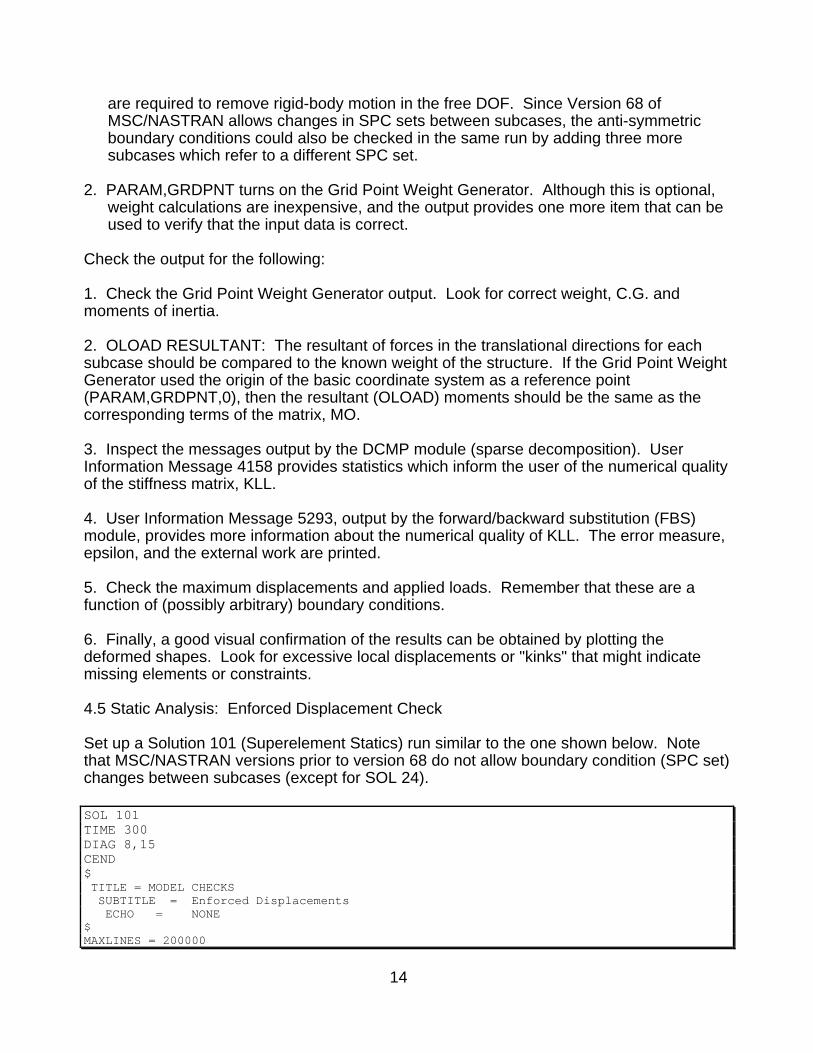
14

are required to remove rigid-body motion in the free DOF. Since Version 68 ofMSC/NASTRAN allows changes in SPC sets between subcases, the anti-symmetricboundary conditions could also be checked in the same run by adding three moresubcases which refer to a different SPC set.

2. PARAM,GRDPNT turns on the Grid Point Weight Generator. Although this is optional,weight calculations are inexpensive, and the output provides one more item that can beused to verify that the input data is correct.

Check the output for the following:

1. Check the Grid Point Weight Generator output. Look for correct weight, C.G. andmoments of inertia.

2. OLOAD RESULTANT: The resultant of forces in the translational directions for eachsubcase should be compared to the known weight of the structure. If the Grid Point WeightGenerator used the origin of the basic coordinate system as a reference point(PARAM,GRDPNT,0), then the resultant (OLOAD) moments should be the same as thecorresponding terms of the matrix, MO.

3. Inspect the messages output by the DCMP module (sparse decomposition). UserInformation Message 4158 provides statistics which inform the user of the numerical qualityof the stiffness matrix, KLL.

4. User Information Message 5293, output by the forward/backward substitution (FBS)module, provides more information about the numerical quality of KLL. The error measure,epsilon, and the external work are printed.

5. Check the maximum displacements and applied loads. Remember that these are afunction of (possibly arbitrary) boundary conditions.

6. Finally, a good visual confirmation of the results can be obtained by plotting thedeformed shapes. Look for excessive local displacements or "kinks" that might indicatemissing elements or constraints.

4.5 Static Analysis: Enforced Displacement Check

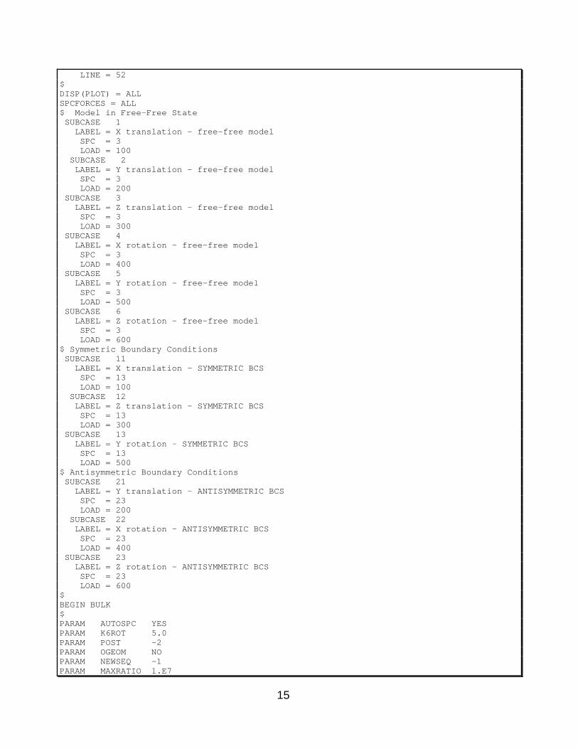
Set up a Solution 101 (Superelement Statics) run similar to the one shown below. Notethat MSC/NASTRAN versions prior to version 68 do not allow boundary condition (SPC set)changes between subcases (except for SOL 24).

SOL 101TIME 300DIAG 8,15CEND$ TITLE = MODEL CHECKS SUBTITLE = Enforced Displacements ECHO = NONE$MAXLINES = 200000

15

LINE = 52$DISP(PLOT) = ALLSPCFORCES = ALL$ Model in Free-Free State SUBCASE 1 LABEL = X translation - free-free model SPC = 3 LOAD = 100 SUBCASE 2 LABEL = Y translation - free-free model SPC = 3 LOAD = 200 SUBCASE 3 LABEL = Z translation - free-free model SPC = 3 LOAD = 300 SUBCASE 4 LABEL = X rotation - free-free model SPC = 3 LOAD = 400 SUBCASE 5 LABEL = Y rotation - free-free model SPC = 3 LOAD = 500 SUBCASE 6 LABEL = Z rotation - free-free model SPC = 3 LOAD = 600$ Symmetric Boundary Conditions SUBCASE 11 LABEL = X translation - SYMMETRIC BCS SPC = 13 LOAD = 100 SUBCASE 12 LABEL = Z translation - SYMMETRIC BCS SPC = 13 LOAD = 300 SUBCASE 13 LABEL = Y rotation - SYMMETRIC BCS SPC = 13 LOAD = 500$ Antisymmetric Boundary Conditions SUBCASE 21 LABEL = Y translation - ANTISYMMETRIC BCS SPC = 23 LOAD = 200 SUBCASE 22 LABEL = X rotation - ANTISYMMETRIC BCS SPC = 23 LOAD = 400 SUBCASE 23 LABEL = Z rotation - ANTISYMMETRIC BCS SPC = 23 LOAD = 600$BEGIN BULK$PARAM AUTOSPC YESPARAM K6ROT 5.0PARAM POST -2PARAM OGEOM NOPARAM NEWSEQ -1PARAM MAXRATIO 1.E7

16

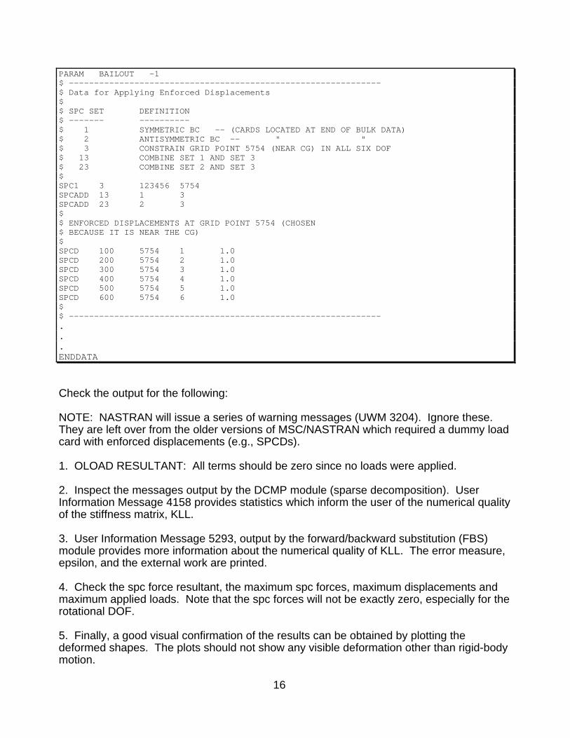
PARAM BAILOUT -1$ --------------------------------------------------------------$ Data for Applying Enforced Displacements$$ SPC SET DEFINITION$ ------- ----------$ 1 SYMMETRIC BC -- (CARDS LOCATED AT END OF BULK DATA)$ 2 ANTISYMMETRIC BC -- " "$ 3 CONSTRAIN GRID POINT 5754 (NEAR CG) IN ALL SIX DOF$ 13 COMBINE SET 1 AND SET 3$ 23 COMBINE SET 2 AND SET 3$SPC1 3 123456 5754SPCADD 13 1 3SPCADD 23 2 3$$ ENFORCED DISPLACEMENTS AT GRID POINT 5754 (CHOSEN$ BECAUSE IT IS NEAR THE CG)$SPCD 100 5754 1 1.0SPCD 200 5754 2 1.0SPCD 300 5754 3 1.0SPCD 400 5754 4 1.0SPCD 500 5754 5 1.0SPCD 600 5754 6 1.0$$ --------------------------------------------------------------...ENDDATA

Check the output for the following:

NOTE: NASTRAN will issue a series of warning messages (UWM 3204). Ignore these.They are left over from the older versions of MSC/NASTRAN which required a dummy loadcard with enforced displacements (e.g., SPCDs).

1. OLOAD RESULTANT: All terms should be zero since no loads were applied.

2. Inspect the messages output by the DCMP module (sparse decomposition). UserInformation Message 4158 provides statistics which inform the user of the numerical qualityof the stiffness matrix, KLL.

3. User Information Message 5293, output by the forward/backward substitution (FBS)module provides more information about the numerical quality of KLL. The error measure,epsilon, and the external work are printed.

4. Check the spc force resultant, the maximum spc forces, maximum displacements andmaximum applied loads. Note that the spc forces will not be exactly zero, especially for therotational DOF.

5. Finally, a good visual confirmation of the results can be obtained by plotting thedeformed shapes. The plots should not show any visible deformation other than rigid-bodymotion.

17

4.6 Static Analysis: Checks Against Reference Data

If data is available from the finite element model developer, a static analysis run can be setup to verify results such as displacements at key locations caused by prescribed forces.The same care should be taken to methodically check the output of such a run, however,the objective is to simply compare results. Since this procedure would vary depending onthe model, no example is given here.

5.0 Summary

Finite element models (FEMs) are the basis for a variety of engineering computations suchas stress and stability analysis, and vibration and dynamic load analysis. Although acarefully developed, thoroughly validated FEM is always desirable, it is of utmostimportance when the model is being used in the preliminary design stages of a largeproject. Since no data is available to validate the model, FEM developers must use theirbest engineering judgment to model the structure accurately. FEM users may want toassess the suitability of the developer's modeling techniques, however a user's primaryvalidation task is to ensure that the model is mathematically correct and does not containany inadvertent errors. This document outlines a suggested procedure for accomplishingthis task.

18

6.0 References

1. "PATRAN Plus User Manual," PDA Engineering, October 1989.

2. "MSC/NASTRAN Reference Manual, Version 68," Lahey, R.S., Miller, M.P. andReymond, M., The MacNeal-Schwendler Corporation, 1994.

3. "I-DEAS Master Series," Structural Dynamics Research Corporation, 1993.

4. "Development and Applications of a Multi-Level Strain Energy Method For DetectingFinite Element Modeling Errors", Hashemi-Kia, M., Kilroy, K., and Parker, G., NASA CR187447, October 1990.

5. "Diagnostics in Finite Element Analysis," Haggenmacher, G.W. and Lahey, R.S., FirstChautauqua on Finite Element Modeling, September 15-17, 1980.

6. "MSC/NASTRAN Linear Static Analysis User's Guide, Version 68," Caffrey, J.P. andLee, J.M., The MacNeal-Schwendler Corporation, 1994.

7. "MSC/NASTRAN Programmer's Manual, Version 64," The MacNeal-SchwendlerCorporation, 1986.

8. "MSC/NASTRAN Numerical Methods User's Guide, Version 67," Komzsik, L., TheMacNeal-Schwendler Corporation, 1992.

9. "MSC/NASTRAN Handbook for Numerical Methods, Version 66," Komszik, L., TheMacNeal-Schwendler Corporation, 1990.