a two-step even–odd split levinson algorithm for toeplitz ...odd levinson algorithm then uses...

Linear Algebra and its Applications 338 (2001) 219–237www.elsevier.com/locate/laa

A two-step even–odd split Levinson algorithmfor Toeplitz systems

A. MelmanDepartment of Mathematics and Computer Science, St. Mary’s College, Moraga, CA 94575, USA

Received 6 March 2001; accepted 22 May 2001

Submitted by H. Schneider

Abstract

We use a two-step Durbin method rather than the single step version in the even–odd splitLevinson algorithm for strongly nonsingular real symmetric Toeplitz systems with arbitraryright-hand side, thereby slightly reducing the complexity of this algorithm to 19

8 n2 + O(n)

flops on a sequential machine. We also present extensive numerical results comparing severalLevinson-type methods. © 2001 Elsevier Science Inc. All rights reserved.

AMS classification: 65F05

Keywords: Toeplitz system; Even–odd structure; Durbin; Levinson; Split Levinson

1. Introduction

The purpose of this work is twofold: to improve an existing algorithm and tonumerically compare a number of similar algorithms.

In the first part, we begin by describing the algorithms to be compared later andthen reduce the complexity of an algorithm, recently proposed in [17], for solvinga strongly nonsingular real symmetric Toeplitz system of linear equations with anarbitrary right-hand side. Such systems are common in many applications, where thematrices involved are positive-definite. This algorithm, the “even–odd splitLevinson” algorithm, is a combination of the “split Durbin” [7] and the “even–oddLevinson” algorithm [16]. The split Durbin algorithm recursively computes the evenand odd solutions of a system with a special right-hand side, namely the Yule–Walker

E-mail address: [email protected] (A. Melman).

0024-3795/01/$ - see front matter � 2001 Elsevier Science Inc. All rights reserved.PII: S 0 0 2 4 - 3 7 9 5 ( 0 1 ) 0 0 3 8 6 - X

220 A. Melman / Linear Algebra and its Applications 338 (2001) 219–237

equations. It does so by solving subsystems of increasing dimension. The even–odd Levinson algorithm then uses these solutions to solve a system with arbitraryright-hand side. However, this algorithm proceeds in steps of two, whereas the splitDurbin algorithm proceeds one step at a time. It would therefore be desirable tohave an algorithm for the Yule–Walker equations which proceeds in steps of two aswell. That this can be done and that this was already implicitly contained in the splitDurbin algorithm was demonstrated in [5]. We will show how this two-step schemecan be incorporated into the even–odd split Levinson algorithm, making it the “two-step even–odd split Levinson algorithm”, which has a slightly lower complexity thanits one-step equivalent, namely 19

8 n2 + O(n) instead of 5

2n2 + O(n) floating point

operations, or flops (following [10], we define a flop, or floating-point operation,as an addition, subtraction, multiplication, or division). However, if two independentprocessors are available, the complexity is reduced to 15

8 n2 + O(n) from 2n2 + O(n)

flops. We do not consider stability issues, even though this new algorithm can be ex-pected to have roughly the same stability properties as the Durbin and split Levinsonalgorithms (see [3] and [14], respectively).

In the second part, we carry out extensive numerical experiments in which wecompare the Levinson-type methods described in the first part. Such studies are notcommonly found in the literature as far as we know and our results point to some-times significant differences between the methods.

Several of the parameters, which appear in the methods we will outline have aspecial meaning in the context of certain applications, such as linear prediction andthe construction of orthogonal polynomials. It would lead us too far to delve into thishere, and we refer to the same references as the ones pointed to in the description ofthe methods where those parameters appear.

The paper is organized as follows. In Section 2 we present some basic defini-tions and results, and then, in Sections 3 and 4, summarize the classical Durbin andLevinson algorithms and their split versions, respectively. In Section 5 the even–oddsplit Levinson algorithm is described, whereas in Sections 6 and 7 we present thetwo-step Durbin algorithm from [5] and show how it can be used to improve thecomplexity of the even–odd split Levinson algorithm. This concludes the first partof the paper. In Section 8, which forms the second part, we present the numericalresults.

2. Preliminaries

A symmetric matrix Tn ∈ R(n,n) is said to be Toeplitz if its elements (Tn)ij satisfy(Tn)ij = ρ|i−j |, where {ρj }n−1

j=0 are the components of a vector (ρ0, tn−1)T ∈ Rn,

with tn−1 = (ρ1, . . . , ρn−1)T ∈ Rn−1, so that

A. Melman / Linear Algebra and its Applications 338 (2001) 219–237 221

Tn =

ρ0 ρ1 ρ2 · · · ρn−1ρ1 ρ0 ρ1 · · · ρn−2...

...... · · · ...

ρn−2 ρn−3 ρn−4 · · · ρ1ρn−1 ρn−2 ρn−3 · · · ρ0

. (1)

Many early results about such matrices can be found in, e.g., [1,2,6,9,11,15]. Theidentity matrix is denoted by I throughout this paper and we will not specificallyindicate its dimension, which is assumed to be clear from the context. We denoteby J the matrix with ones on its southwest–northeast diagonal and zeros everywhereelse (the exchange matrix). As with I, we will not specifically indicate its dimension.

Toeplitz matrices are persymmetric, i.e., they are symmetric about their south-west–northeast diagonal. For such a matrix Tn, this is the same as requiring thatJT T

n J = Tn. It is easy to see that the inverse of a persymmetric matrix is also per-symmetric. A matrix that is both symmetric and persymmetric is called doubly sym-metric.

An even (sometimes also referred to as symmetric) vector v is defined as a vectorsatisfying Jv = v and an odd (sometimes called antisymmetric or skew-symmetric)vector w as one that satisfies Jw = −w.

Throughout this paper, it will be assumed that the matrix Tn is strongly nonsingu-lar, i.e., that its principal submatrices Tk , k = 1, 2, . . . , n, are all nonsingular.

3. The Durbin and Levinson algorithms

We now briefly present both Durbin’s and Levinson’s algorithms, referring to [10,pp. 194–196] and [17] for full details.

3.1. Durbin’s algorithm

The Yule–Walker equations we referred to in the introduction are given byTny

(n) = −tn, where Tn is as in (1) and tk = (ρ1, . . . , ρk)T. Durbin’s algorithm

solves this system recursively as follows: assuming that the solution to Tk−1y(k−1) =

−tk−1 is available, compute the solution to Tky(k) = −tk from

y(k)j =y(k−1)

j + αk−1

(Jy(k−1)

)j

(1 � j � k − 1), (2)

y(k)k =αk−1, (3)

with

αk−1 = −ρk + tTk−1Jy(k−1)

ρ0 + tTk−1y(k−1)

. (4)


The strong nonsingularity of Tn ensures that the denominator in (4) is never zero.The magnitude of this denominator affects the numerical accuracy.

In addition, we define βk = ρ0 + tTk y(k). The following recursion then holds (see[10, p. 195]):

βk = (1 − α2k−1)βk−1. (5)

Because of the strong nonsingularity assumption on Tn, βk /= 0, and therefore αk /=1.The first step of the method consists of solving a trivial 1 × 1 system, whereas in

the final step, y(n) is computed from y(n−1), βn−1, and αn−1. The quantities αk arecalled reflection coefficients, or Schur–Szegö parameters.

Complexity. This algorithm requires a total of n2 + O(n) additions and n2 + O(n)multiplications, or 2n2 + O(n) flops.

3.2. Levinson’s algorithm

We now turn to Levinson’s algorithm for solving the general right-hand side prob-lem Tny

(n) = b(n), with b(k) = (b1, b2, . . . , bk)T. It solves this system recursively

as follows: assuming that the solutions to Tk−1x(k−1) = b(k−1) and Tk−1y

(k−1) =−tk−1 are available, the algorithm computes the solution to Tkx(k) = b(k) from:

x(k)j =x(k−1)

j + µk−1

(Jy(k−1)

)j

(1 � j � k − 1), (6)

x(k)k =µk−1, (7)

with

µk−1 = bk − tTk−1Jx(k−1)

ρ0 + tTk−1y(k−1)

. (8)

As was mentioned before, the denominator in (8) is nonzero for a strongly non-singular Tn, so that µk is well-defined. Durbin’s algorithm is used “in parallel” forcomputing the solutions y(k) of the Yule–Walker subsystems.

Complexity. Taking into account the complexity of Durbin’s algorithm, this algo-rithm requires a total of 2n2 + O(n) additions and 2n2 + O(n) multiplications, or4n2 + O(n) flops.

4. The split Durbin and split Levinson algorithms

The “split Levinson” algorithms for the Yule–Walker equations and for the gener-al case, were introduced in [7] and [8], respectively. However, in the spirit of Goluband Van Loan [10], we will call the split Levinson algorithm for Yule–Walker equa-tions from [7], the “split Durbin algorithm”, to distinguish it from the split Levinsonalgorithm for the general right-hand side case in [8]. We will also use the formulation


of these algorithms as they were presented in [17], to which we once again refer forthe details.

4.1. The split Durbin algorithm for the Yule–Walker equations

We start with the split Levinson algorithm from [7] for the Yule–Walker equa-tions Tny(n) = −tn, from now on called the “split Durbin” algorithm. Defining aneven solution u(k) of these equations as the solution of Tku(k) = −(tk + J tk), oru(k) = y(k) + Jy(k) and an odd solution as the solution of Tkv(k) = −(tk − J tk),or v(k) = y(k) − Jy(k), this algorithm is based on the remarkable observation thatthe solution y(k) can be written either as a combination of the two successive evensolutions u(k) and u(k−1) or as a combination of the two successive odd solutions v(k)

and v(k−1). It is therefore sufficient to compute either the even or the odd solutions.As we shall see, this can be achieved with fewer operations than Durbin’s algorithm.

In what follows, we concentrate on the even solutions and refer to [7] for thecorresponding (and analogous) results for the odd solutions.

The split Durbin algorithm solves for the even solutions as follows: assuming thatthe solutions to Tk−1u

(k−1) = −(tk−1 + J tk−1) and Tk−2u(k−2) = −(tk−2 + J tk−2)

are available, compute, for k = 1, . . . , n, the solution to Tku(k) = −(tk + J tk) from:

u(k)1 =u(k)k = u(k−1)

1 − γk−1

γk−2+ 1, (9)

u(k)j =u(k−1)

j + u(k−1)j−1 −

(γk−1

γk−2

)u(k−2)j−1 (2 � j � k − 1). (10)

After this, compute y(n) from

y(n)1 =u(n)1 − αn−1,

y(n)j =y(n)j−1 + u(n)j − (1 + αn−1)u

(n−1)j−1 (2 � j � n).

All necessary quantities for k = 1, 2 are easily computed before starting the algo-rithm.

The following relations hold:

αk−1 =∑kj=1 u

(k)j −∑k−1

j=1 u(k−1)j

2 +∑k−1j=1 u

(k−1)j

, (11)

γk=ρ0 + tTk u(k) + ρk+1. (12)

(We note that the letters p and q in λpk−2 and λqk−2 are superscripts, not exponents.)The denominator in (11) and the expression in (12) are nonzero because of the strongnonsingularity assumption on Tn. The magnitude of these quantities affects the ac-curacy of the algorithm. The full details for this method can be found in [17].

Complexity. The total number of operations required by the algorithm is n2 +O(n) additions and 1

2n2 + O(n) multiplications, or 3

2 n2 + O(n) flops.


4.2. The split Levinson algorithm for the general case

We now turn to the general right-hand side problem Tnx(n) = b(n), where b(k) =

(b1, . . . , bk)T. We define the even vectors s(k) = b(k) + Jb(k) for k = 1, . . . , n. We

also define an even solution w(k) as the solution of Tkw(k) = s(k), or w(k) = x(k) +Jx(k). As in the case of the Yule–Walker equations, the solution x(k) can be written interms of the two successive even solutions w(k) and w(k−1). It is therefore sufficient,once again, to compute only the even solutions, which requires fewer operationsthan Levinson’s algorithm. Analogous results exist for the odd solutions, but we willdiscuss only the even case, as this is the case we will need later. The split Levinsonalgorithm solves for the even solutions as follows: assuming that the solutions toTk−1u

(k−1) = −(tk−1 + J tk−1), Tk−2u(k−2) = −(tk−2 + J tk−2), Tk−1w

(k−1) =b(k−1) + Jb(k−1), and Tk−2w

(k−2) = b(k−2) + Jb(k−2) are available, compute, fork = 3, . . . , n, the solution to Tku(k) = −(tk + J tk) using the split Durbin algorithmand the solution to Tkw(k) = b(k) + Jb(k) from:

w(k)1 = w(k)k = w(k−1)

1 − tTk−1w(k−1) − tTk−2w

(k−2) − bk + bk−1

ρ0 + tTk−2u(k−2) + ρk−1

, (13)

w(k)j =w(k−1)

j + w(k−1)j−1 − w(k−2)

j−1

−(tTk−1w

(k−1) − tTk−2w(k−2) − bk + bk−1

ρ0 + tTk−2u(k−2) + ρk−1

)u(k−2)j−1

(2 � j � k − 1). (14)

After this, compute x(n) from

x(n)1 =w(n)1 − µn−1,

x(n)j =x(n)j−1 + w(n)j − w(n−1)

j−1 − µn−1u(n−1)j−1 (2 � j � n).

All necessary quantities for k = 1, 2 are easily computed before starting the algo-rithm.

The following relation holds:

µk−1 =∑kj=1w

(k)j −∑k−1

j=1w(k−1)j

2 +∑k−1j=1 u

(k−1)j

, (15)

which is, once again, well-defined because of the strong nonsingularity assumptionon Tn.

Complexity. Taking into account the complexity of the split Durbin’s algorithm forthe Yule–Walker equations, the algorithm requires a total of 2n2 + O(n) additionsand n2 + O(n) multiplications, or 3n2 + O(n) flops.


5. The even–odd split Levinson algorithm

In this section we describe the “even–odd split Levinson algorithm”, a combi-nation of the split Durbin algorithm with the “even–odd Levinson algorithm” from[16]. The details can be found in [17]. Before we state this algorithm, we need thefollowing definitions:

p(k)=(s(n)

n−k2 �+1, . . . , s

(n)

n+k2 �

)T

,

q(k)=(s(n−2) n−k2 �, . . . , s

(n−2) n+k2 �−1

)T

,

h(k)p =T −1k p(k),

h(k)q =T −1k q(k).

This means that p(n) = s(n), q(n−2) = s(n−2), h(n)p = w(n), and h(n−2)q = w(n−2).

For k = 4, 6, . . . , n− 2 (n even) or k = 3, 5, 7, . . . , n− 2 (n odd), the algorithmproceeds as follows: assuming that h(k−2)

p , h(k−2)q , u(k−1), and u(k−2) are available,

compute u(k) with the split Durbin algorithm and compute h(k)p , h(k)q from:

(h(k)p

)1 =(h(k)p )k = λpk−2, (16)(

h(k)p)j=(h(k−2)

p

)j

+ λpk−2

(u(k−2))

j(2 � j � k − 1) (17)

and

(h(k)q

)1 =(h(k)q )k = λqk−2, (18)(

h(k)q)j=(h(k−2)

q

)j

+ λqk−2

(u(k−2))

j(2 � j � k − 1), (19)

with

λp

k−2 =s(n)

n−k2 �+1− tTk−2h

(k−2)p

ρ0 + tTk−2u(k−2) + ρk−1

, (20)

λq

k−2 =s(n−2) n−k2 � − tTk−2h

(k−2)q

ρ0 + tTk−2u(k−2) + ρk−1

. (21)

This produces h(n−2)q = w(n−2). Perform (16) and (17) once more, for k = n, to

obtain h(n)p = w(n). The algorithm is initialized by solving a trivial 1 × 1 or 2 × 2system, depending on whether n is odd or even, respectively.


Let us now show how we can compute the remaining quantities, necessary tocalculate x(n), in O(n) operations. We start by computing w(n−1) from w(n) andw(n−2). From (13) and (14), we have

w(n−1)1 =w(n)1 + η, (22)

w(n−1)j =−w(n−1)

j−1 + w(n)j + w(n−2)j−1 + ηu(n−2)

j−1 (2 � j � n− 1), (23)

where

η = tTn−1w(n−1) − tTn−2w

(n−2) − bn + bn−1

ρ0 + tTn−2u(n−2) + ρn−1

. (24)

To compute w(n−1), we first compute η, for which we use the fact that

tTn−1w(n−1)= tTn−1T

−1n−1(b

(n−1) + Jb(b−1))

=(tn−1 + J tn−1)TT −1n−1b

(n−1)

=−(u(n−1))Tb(n−1).

The remaining components of w(n−1) then follow from (23). We note that the de-nominators in (20), (21) and (24) are all nonzero because of the strong nonsingularityassumption on Tn and that their magnitude affects the accuracy of the algorithm.

Finally, we compute µn−1 from (15) and obtain for the solution x(n):

x(n)1 =w(n)1 − µn−1,

x(n)j =−x(n)j−1 + w(n)j − w(n−1)

j−1 − µn−1u(n−1)j−1 (2 � j � n).

Therefore, the computation of w(n−1) and, subsequently, of x(n), requires an ad-ditional O(n) flops.

We conclude the description of this algorithm by noting that we used the evensolutions to obtain the general solution. It would not be possible to do the same withthe odd solutions, because the reflection coefficients µk are not computed by theeven–odd Levinson algorithm. In the even case this is not necessary because we canobtain these also from (15), as we did at the end of the algorithm, when we calculatedµn−1 to obtain the general solution. However, (15) has no analog in the odd case. Ofcourse, if one only wants to compute the odd solution, without computing the generalsolution, then the reflection coefficients are not necessary.

Complexity. Taking into account the complexity of the split Durbin algorithm,the complexity of this algorithm is 3

2n2 + O(n) additions and n2 + O(n) multipli-

cations, or 52 n2 + O(n) flops on a sequential machine. However, if two independent

processors are available, this complexity is reduced to 2n2 + O(n) flops (see [17]).


6. The two-step split Durbin and two-step even–odd split Levinson algorithms

In this section, we derive a two-step split Durbin algorithm, which we then com-bine with the even–odd Levinson algorithm from [16]. This in itself is not new (see[5]): what is new is the resulting algorithm, which is different from the even–odd splitLevinson algorithm in [17], where the even–odd Levinson algorithm was combinedwith the one-step split Durbin algorithm from [7]. The result is a method with a lowercomplexity and a different numerical behavior.

6.1. The two-step split Durbin algorithm

We first derive a two-step version of the split Durbin algorithm. This same versionof the algorithm can also be found in [5], albeit in slightly different notation. In fact,this algorithm is implicitly contained in the split Durbin algorithm, as will becomeclear from its derivation.

Using Eq. (10) for u(k−1)j and u(k−1)

j−1 instead of u(k)j for 3 � j � k − 1 and com-bining the two yields:

u(k−1)j + u(k−1)

j−1 =u(k−2)j + 2u(k−2)

j−1 + u(k−2)j−2

−γk−2

γk−3

(u(k−3)j−1 + u(k−3)

j−2

). (25)

On the other hand, Eq. (10), with k − 2 instead of k, gives

u(k−3)j−1 + u(k−3)

j−2 = u(k−2)j−1 +

(γk−3

γk−4

)u(k−4)j−2 . (26)

Combining (26) with (25) and substituting back in (10) yields

u(k)j =u(k−2)

j +(

2 − γk−1

γk−2− γk−2

γk−3

)u(k−2)j−1 + u(k−2)

j−2

−(γk−2

γk−4

)u(k−4)j−2 . (27)

To examine the coefficient of u(k−2)j−1 , we will consider the quantity 1 − (γk−1/γk−2)

in more detail. We have

1 − γk−1

γk−2= γk−2 − γk−1

γk−2= tTk−2u

(k−2) − tTk−1u(k−1) + ρk−1 − ρk

γk−2. (28)

Defining t̄k =(ρ2, . . . , ρk+1)

T, using k − 1 instead of k in (10) and using the evenproperties of the vectors u(k−1) and u(k−2) allow us to write tTk−1u

(k−1) as

tTk−1u(k−1)=

k−1∑j=1

ρju(k−1)j = (ρ1 + ρk−1) u

(k−1)1 +

k−2∑j=2

ρju(k−1)j


=(ρ1 + ρk−1)

(u(k−2)1 − γk−2

γk−3+ 1

)+k−2∑j=2

ρj

(u(k−2)j + u(k−2)

j−1

)

−γk−2

γk−3

k−2∑j=2

ρju(k−3)j−1

=ρk−1u(k−2)1 + (ρ1 + ρk−1)

(1 − γk−2

γk−3

)+ tTk−2u

(k−2)

+(t̄ Tk−2u

(k−2) − ρk−1u(k−2)k−2

)−(γk−2

γk−3

)t̄ Tk−3u

(k−3)

=ρ1 + ρk−1 + tTk−2u(k−2) + t̄ T

k−2u(k−2)

−γk−2

γk−3

(ρ1 + ρk−1 + t̄ T

k−3u(k−3)

).

Substituting this back into (28) gives

1 − γk−1

γk−2= −ρ1 + ρk + t̄ T

k−2u(k−2)

γk−2+ ρ1 + ρk−1 + t̄ T

k−3u(k−3)

γk−3. (29)

We define

δk = ρ1 + t̄ T

k u(k) + ρk+2,

so that, with the help of (29), we obtain

2 − γk−1

γk−2− γk−2

γk−3=(

1 − γk−1

γk−2

)+(

1 − γk−2

γk−3

)= − δk−2

γk−2+ δk−4

γk−4·

Since the quantities, related to the (k − 3)th subsystem, have dropped out, this makesit now possible for the algorithm to advance in steps of two. Proceeding analogouslyfor the first two components of u(k), we can formulate the basis for the two-step splitDurbin algorithm as follows:

u(k)1 =u(k)k = u(k−2)

1 − δk−2

γk−2+ δk−4

γk−4, (30)

u(k)2 =u(k−2)

2 +(δk−4

γk−4− δk−2

γk−2

)− γk−2

γk−4+ 1, (31)

u(k)j =u(k−2)

j +(δk−4

γk−4− δk−2

γk−2

)u(k−2)j−1 + u(k−2)

j−2

−(γk−2

γk−4

)u(k−4)j−2 (3 � j � k − 1). (32)

Complexity. At each step this algorithm computes two scalar products involvingan even vector, and an update. Taking into account that it progresses in steps oftwo and that roughly only half of the components need to be computed (as with the


other split methods), one finds that a total of 78n

2 + O(n) additions and 12n

2 + O(n)multiplications are executed. The complexity is therefore 11

8 n2 + O(n) flops.

6.2. The two-step even–odd split Levinson algorithms

The new algorithm we now propose uses the two-step split Durbin algorithm tocompute the successive even solutions of the Yule–Walker equations in the even–oddsplit Levinson method. Therefore, this method, which we call the “two-step even–odd split Levinson algorithms”, “leaps over” subsystems of even or odd dimensions,when the dimension n of the system Tnx(n) = b(n) that we are solving is odd or even,respectively.

The recursive process in this case no longer provides us with u(n−1) as in theregular even–odd split Levinson method, but this quantity still needs to be calculatedbefore x(n) can be computed. Once u(n−1) is available, x(n) is obtained exactly as inthe even–odd split Levinson algorithm.

The computation of u(n−1) can be done with (9) and (10) for k = n− 1, namely:

u(n−1)1 =u(n−1)

n−1 = u(n−2)1 − γn−2

γn−3+ 1,

u(n−1)j =u(n−2)

j + u(n−2)j−1 − γn−2

γn−3u(n−3)j−1 (2 � j � n− 2),

provided we can compute u(n−3). This in turn can be achieved by considering onceagain (9) and (10), this time for k = n− 2, which yields

u(n−3)1 =u(n−2)

1 + γn−3

γn−4− 1,

u(n−3)j =−u(n−3)

j−1 + u(n−2)j +

(γn−3

γn−4

)u(n−4)j−1 (2 � j � n− 3).

The only unknown quantity in these expressions is γn−3/γn−4. To compute it, weconsider the following:

k−1∑j=2

(−1)ju(k)j =k−1∑j=2

(−1)j (u(k−1)j + u(k−1)

j−1 )−γk−1

γk−2

k−1∑j=2

(−1)ju(k−2)j−1

=k−1∑j=2

(−1)ju(k−1)j +

k−2∑j=1

(−1)j−1u(k−1)j

−γk−1

γk−2

k−2∑j=1

(−1)j−1u(k−2)j


=(−1)k−1u(k−1)k−1 + u(k−1)

1 +k−2∑j=2

((−1)j + (−1)j−1

)u(k−1)j

−γk−1

γk−2

k−2∑j=1

(−1)j−1u(k−2)j

=(

1 + (−1)k−1)u(k−1)1 − γk−1

γk−2

k−2∑j=1

(−1)j−1u(k−2)j .

Recalling that

u(k)1 = u(k−1)

1 − γk−1

γk−2+ 1,

we have

(1 + (−1)k−1

)+

k∑j=1

(−1)ju(k)j

= γk−1

γk−2

(1 + (−1)k−1

)+k−2∑j=1

(−1)ju(k−2)j

.

Because u(k) and u(k−2) are even vectors, this expression is useless when k is even, inwhich case it reduces to 0 = 0. However, when k is odd, it provides us with a usefulequation, namely

2 +∑kj=1(−1)ju(k)j

2 +∑k−2j=1(−1)ju(k−2)

j

= γk−1

γk−2.

Setting k = n− 2 then yields a computable expression for γn−3/γn−4. We remarkthat this procedure is also used in [12]. Once again, the denominators in this expres-sion can be shown to be nonzero because of the strong nonsingularity assumption onthe coefficient matrix Tn.

Therefore, when n is odd, we compute the solution x(n) by using the even–oddsplit Levinson algorithm with the two-step split Durbin algorithm for the Yule–Walk-er equations. When n is even, we compute first the solution of Tn−1x

(n−1) = b(n−1)

as was just outlined (since in this case n− 1 is odd), and then carry out one step ofthe Levinson algorithm to compute x(n). We note that the last part of the algorithm,namely the computation of u(n−3), u(n−1), and subsequently of x(n), requires O(n)flops.

Complexity. Taking into account the complexity of the two-step Durbin algo-rithm, a total of 11

8 n2 + O(n) additions and n2 + O(n) multiplications are carried

out, which yields a complexity of 198 n2 + O(n) flops on a sequential machine. How-


ever, if two independent processors are available, the complexity is reduced exactlyas in the even–odd split Levinson method: in this case it becomes 15

8 n2 + O(n) flops.

7. Summary

Table 1 contains the number of floating point operations needed by the differentmethods described in this work to solve an aribitrary right-hand side problem on asequential machine. We have denoted the Levinson, split Levinson, even–odd splitLevinson and two-step even–odd split Levinson algorithms by L, SL, EOSL, andTSEOSL, respectively. In Fig. 1, we have plotted the number of flops as a functionof the dimension of the problem for each of the aforementioned algorithms. Theleading term in the complexity is clearly reflected in the plots. However, the relativeperformances of the methods may vary slightly in different implementations. In ours,we achieved the following ranking:

15 � n � 25: Flops(TSEOSL) > Flops(L) > Flops(SL) > Flops(EOSL)

25 < n � 45: Flops(L) > Flops(TSEOSL) > Flops(SL) > Flops(EOSL)

45 < n � 210: Flops(L) > Flops(SL) > Flops(TSEOSL) > Flops(EOSL)

n > 210: Flops(L) > Flops(SL) > Flops(EOSL) > Flops(TSEOSL)

For n < 15, the differences are not significant. This ranking makes it easy to identifythe curves in the plot.

8. Numerical results

8.1. Test matrices

We have tested these methods on three classes of matrices, two of which are class-es of positive-definite matrices. These were randomly generated, and even thoughthis usually tends to avoid seriously ill-conditioned matrices, it is sufficient for thepurpose of comparing the methods. For each class we have made three comparisons,

Table 1Comparison of the complexity of methods for an arbitrary right-hand side problem

Method Additions Multiplications Total number of flops

L 2n2 + O(n) 2n2 + O(n) 4n2 + O(n)

SL 2n2 + O(n) n2 + O(n) 3n2 + O(n)

EOSL 32n

2 + O(n) n2 + O(n) 52n

2 + O(n)

TSEOSL 118 n

2 + O(n) n2 + O(n) 198 n

2 + O(n)


Fig. 1 The number of flops as a function of the dimension of the problem for the four methods.

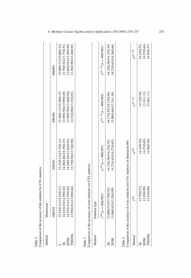
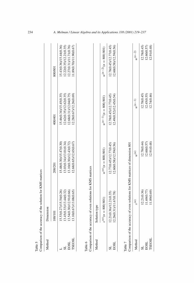
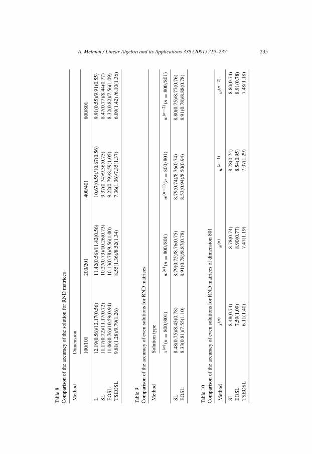
and collected the results in Tables 2–10. Tables 2, 5 and 8 compare the averagerelative accuracy of the solution of Tnx(n) = b(n) for the four methods and for the di-mensions n = 100, 101, 200, 201, 400, 401, 800, 801. In each of its columns under-neath the dimension one finds the average value of the quantity − log10(‖Tnx(n) −b(n)‖/‖x(n)‖), with its standard deviation in parentheses, obtained from 4000 ran-domly generated problems. Each entry contains two such results, separated by aslash and corresponding to the dimensions in the column heading.

Tables 3, 6 and 9 compare the average accuracy of x(n), w(n), w(n−1), and w(n−2)

for n = 800 and n = 801 for the SL and EOSL methods.Tables 4, 7 and 10 compare the average accuracy of x(n),w(n),w(n−1), andw(n−2)

for n = 801 for the SL, EOSL and TSEOSL algorithms.Tables 3, 6, 9 and 4, 7, 10 use the same format as Tables 2, 5 and 8 and are

each based on 4000 randomly generated problems. We now list the three classes ofmatrices.

(1) CVL matrices. These are matrices defined in [4] (whence their name) as

T = µn∑k=1

ξkT2πθk ,

where n is the dimension of T, µ is such that Tkk = 1, k = 1, . . . , n, and

(Tθ )ij = cos(θ(i − j)).These matrices are positive semi-definite. We generated random matrices of this kindby taking the value of θk to be uniformly distributed on (0, 1).

A. Melman / Linear Algebra and its Applications 338 (2001) 219–237 233Ta

ble

2C

ompa

riso

nof

the

accu

racy

ofth

eso

lutio

nfo

rC

VL

mat

rice

s

Met

hod

Dim

ensi

on

100/

101

200/

201

400/

401

800/

801

L15

.43(

0.11

)/15

.43(

0.11

)15

.32(

0.11

)/15

.32(

0.11

)15

.20(

0.11

)/15

.20(

0.12

)15

.08(

0.11

)/15

.08(

0.12

)SL

14.4

1(0.

43)/

14.3

9(0.

42)

14.2

0(0.

46)/

14.1

9(0.

47)

13.9

9(0.

50)/

13.9

9(0.

49)

13.7

9(0.

52)/

13.7

7(0.

51)

EO

SL14

.33(

0.51

)/13

.79(

0.85

)14

.16(

0.54

)/13

.62(

0.91

)13

.99(

0.59

)/13

.46(

0.94

)13

.86(

0.61

)/13

.30(

0.96

)T

SEO

SL13

.95(

0.81

)/13

.89(

0.84

)13

.77(

0.89

)/13

.72(

0.90

)13

.57(

0.90

)/13

.57(

0.93

)13

.39(

0.99

)/13

.40(

0.95

)

Tabl

e3

Com

pari

son

ofth

eac

cura

cyof

even

solu

tions

for

CV

Lm

atri

ces

Met

hod

Solu

tion

type

x(n)(n

=80

0/80

1)w(n) (n

=80

0/80

1)w(n

−1)(n

=80

0/80

1)w(n

−2) (n

=80

0/80

1)

SL13

.80(

0.51

)/13

.79(

0.52

)14

.13(

0.56

)/14

.15(

0.55

)14

.17(

0.55

)/14

.11(

0.56

)14

.12(

0.56

)/14

.15(

0.55

)E

OSL

13.8

6(0.

62)/

13.2

8(0.

99)

14.2

7(0.

65)/

14.2

7(0.

65)

13.9

0(0.

66)/

13.3

1(1.

10)

14.2

7(0.

65)/

14.2

6(0.

66)

Tabl

e4

Com

pari

son

ofth

eac

cura

cyof

even

solu

tions

for

CV

Lm

atri

ces

ofdi

men

sion

801

Met

hod

x(n)

w(n)

w(n

−1)

w(n

−2)

SL13

.79(

0.51

)14

.15(

0.54

)14

.12(

0.56

)14

.15(

0.55

)E

OSL

13.2

9(0.

99)

14.2

7(0.

65)

13.3

1(1.

12)

14.2

7(0.

66)

TSE

OSL

13.4

1(0.

98)

14.4

6(0.

56)

13.4

8(1.

11)

14.4

5(0.

57)

234 A. Melman / Linear Algebra and its Applications 338 (2001) 219–237Ta

ble

5C

ompa

riso

nof

the

accu

racy

ofth

eso

lutio

nfo

rK

MS

mat

rice

s

Met

hod

Dim

ensi

on

100/

101

200/

201

400/

401

800/

801

L15

.53(

0.27

)/15

.54(

0.26

)15

.48(

0.30

)/15

.47(

0.30

)15

.46(

0.34

)/15

.45(

0.35

)15

.43(

0.36

)/15

.44(

0.36

)SL

13.4

5(0.

33)/

13.4

4(0.

32)

13.0

3(0.

34)/

13.0

1(0.

34)

12.6

2(0.

35)/

12.6

2(0.

35)

12.2

2(0.

35)/

12.2

1(0.

35)

EO

SL13

.54(

0.30

)/12

.91(

0.66

)13

.10(

0.30

)/12

.43(

0.72

)12

.68(

0.31

)/12

.04(

0.75

)12

.27(

0.31

)/11

.71(

0.76

)T

SEO

SL13

.10(

0.67

)/13

.08(

0.65

)12

.68(

0.65

)/12

.65(

0.67

)12

.28(

0.67

)/12

.26(

0.69

)11

.89(

0.70

)/11

.90(

0.67

)

Tabl

e6

Com

pari

son

ofth

eac

cura

cyof

even

solu

tions

for

KM

Sm

atri

ces

Met

hod

Solu

tion

type

x(n)(n

=80

0/80

1)w(n) (n

=80

0/80

1)w(n

−1)(n

=80

0/80

1)w(n

−2) (n

=80

0/80

1)

SL12

.21(

0.36

)/12

.21(

0.35

)12

.77(

0.45

)/12

.77(

0.45

)12

.78(

0.45

)/12

.77(

0.45

)12

.78(

0.45

)/12

.77(

0.45

)E

OSL

12.2

6(0.

31)/

11.6

7(0.

78)

12.6

0(0.

58)/

12.5

9(0.

56)

12.4

9(0.

52)/

12.4

5(0.

54)

12.6

0(0.

58)/

12.5

9(0.

56)

Tabl

e7

Com

pari

son

ofth

eac

cura

cyof

even

solu

tions

for

KM

Sm

atri

ces

ofdi

men

sion

801

Met

hod

x(n)

w(n)

w(n

−1)

w(n

−2)

SL12

.21(

0.36

)12

.78(

0.44

)12

.78(

0.45

)12

.78(

0.45

)E

OSL

11.6

9(0.

77)

12.6

0(0.

57)

12.4

5(0.

55)

12.6

0(0.

57)

TSE

OSL

11.8

9(0.

69)

12.9

1(0.

48)

12.7

4(0.

46)

12.9

1(0.

48)

A. Melman / Linear Algebra and its Applications 338 (2001) 219–237 235Ta

ble

8C

ompa

riso

nof

the

accu

racy

ofth

eso

lutio

nfo

rR

ND

mat

rice

s

Met

hod

Dim

ensi

on

100/

101

200/

201

400/

401

800/

801

L12

.19(

0.56

)/12

.17(

0.56

)11

.42(

0.56

)/11

.42(

0.56

)10

.67(

0.55

)/10

.67(

0.56

)9.

91(0

.55)

/9.9

1(0.

55)

SL11

.17(

0.72

)/11

.17(

0.72

)10

.27(

0.73

)/10

.26(

0.73

)9.

37(0

.74)

/9.3

6(0.

75)

8.47

(0.7

7)/8

.44(

0.77

)E

OSL

11.0

6(0.

76)/

10.5

9(0.

94)

10.1

3(0.

78)/

9.56

(1.0

0)9.

22(0

.79)

/8.5

9(1.

05)

8.32

(0.8

2)/7

.56(

1.09

)T

SEO

SL9.

81(1

.28)

/9.7

9(1.

26)

8.55

(1.3

6)/8

.52(

1.34

)7.

36(1

.36)

/7.3

5(1.

37)

6.09

(1.4

2)/6

.10(

1.36

)

Tabl

e9

Com

pari

son

ofth

eac

cura

cyof

even

solu

tions

for

RN

Dm

atri

ces

Met

hod

Solu

tion

type

x(n)(n

=80

0/80

1)w(n) (n

=80

0/80

1)w(n

−1) (n

=80

0/80

1)w(n

−2) (n

=80

0/80

1)

SL8.

48(0

.75)

/8.4

5(0.

78)

8.79

(0.7

5)/8

.76(

0.75

)8.

79(0

.74)

/8.7

6(0.

74)

8.80

(0.7

5)/8

.77(

0.76

)E

OSL

8.33

(0.8

1)/7

.55(

1.10

)8.

91(0

.78)

/8.8

7(0.

78)

8.53

(0.9

4)/8

.50(

0.94

)8.

91(0

.78)

/8.8

8(0.

78)

Tabl

e10

Com

pari

son

ofth

eac

cura

cyof

even

solu

tions

for

RN

Dm

atri

ces

ofdi

men

sion

801

Met

hod

x(n)

w(n)

w(n

−1)

w(n

−2)

SL8.

48(0

.74)

8.78

(0.7

4)8.

78(0

.74)

8.80

(0.7

4)E

OSL

7.59

(1.0

9)8.

90(0

.77)

8.54

(0.9

5)8.

91(0

.78)

TSE

OSL

6.11

(1.4

0)7.

47(1

.19)

7.07

(1.2

9)7.

48(1

.18)


(2) KMS matrices. These are the Kac–Murdock–Szegö matrices (see [13]), de-fined as

Tij = ν|i−j |,

where 0 < ν < 1 and i, j = 1, . . . , n, where n is the dimension of the matrix. Theyare positive definite. Random matrices of this kind were generated by taking thevalue of ν to be uniformly distributed on (0, 1).

(3) RND matrices. We define RND matrices by defining a random vector v oflength n whose components are uniformly distributed on (0, 1).

Theoretically, some of the matrices generated in the experiments might not bestrongly nonsingular, although we never encountered this situation in practice.

All experiments were implemented in MATLAB.

8.2. Conclusions

First of all, there is a marked difference in accuracy between positive definite sys-tems and those that are not: all algorithms achieve a much higher accuracy for posi-tive definite systems. This is not unexpected as the stability results that are availablefor these methods [3,14] are all derived under the assumption of positive definiteness.

In the case of our particular test problems there is also a substantial differencebetween systems of even and odd dimension for the EOSL algorithm, reflected notonly in the accuracy, but also in the standard deviation: systems of odd dimensionyield a lower accuracy and higher standard deviation. We found no satisfactory ex-planation for this phenomenon nor do we know how general it is. This is only truefor the accuracy of x(n): there was no such difference for the even solutions w(n) andw(n−2). Only for CVL matrices is there a difference in accuracy for w(n−1) betweeneven and odd dimensions, not for KMS and RND matrices. It seems clear that someaccuracy is lost when quantities have to be reconstructed, as opposed to when theyare computed recursively. This is especially true for the TSEOSL algorithm, whereseveral quantities need to be reconstructed in addition to x(n), namely µn−1, u(n−3),u(n−1), and w(n−1). This algorithm displays virtually no difference between evenand odd dimensions because it basically always solves a problem of odd dimension.However, the quantities that are computed recursively by the TSEOSL algorithmdo not suffer from this and are computed to higher accuracy than both the SL andEOSL algorithms for both classes of positive-definite matrices, but not for the RNDmatrices. This seems to indicate that this method is best suited for implementationon two independent processors, where the even and odd solutions are computed sep-arately: in such a case the method seems capable of maintaining high accuracy whilereducing the flop count, except for indefinite matrices.

As is clear from the results, the Levinson algorithm achieved the highest accura-cy and smallest standard deviation for our particular problems. The SL and EOSLalgorithms performed fairly similarly, except when the dimension of the system was


odd, in which case the SL algorithm was superior. As was mentioned before, theTSEOSL algorithm’s accuracy was superior to that of the SL and EOSL algorithmsfor the even solutions in the case of positive-definite matrices, while this was nottrue for the solution of the system itself. The accuracy decreased with increasingdimension of the system for all methods, although the Levinson algorithm was leastaffected by this.

References

[1] A.L. Andrew, Eigenvectors of certain matrices, Linear Algebra Appl. 7 (1973) 151–162.[2] A. Cantoni, F. Butler, Eigenvalues and eigenvectors of symmetric centrosymmetric matrices, Linear

Algebra Appl. 13 (1976) 275–288.[3] G. Cybenko, The numerical stability of the Levinson–Durbin algortihm for Toeplitz systems of equa-

tions, SIAM J. Sci. Statist. Comput. 1 (1980) 303–319.[4] G. Cybenko, C. Van Loan, Computing the minimum eigenvalue of a symmetric positive definite

Toeplitz matrix, SIAM J. Sci. Statist. Comput. 7 (1) (1986) 123–131.[5] C.J. Demeure, Bowtie factors of Toeplitz matrices by means of split algorithms, IEEE Trans. Acoust.

Speech, Signal Process. 37 (10) (1989) 1601–1603.[6] P. Delsarte, Y. Genin, Spectral properties of finite Toeplitz matrices, in: Mathematical Theory of

Networks and Systems, Proc. MTNS-83 International Symposium, Beer-Sheva, Israel, 1983, pp.194–213.

[7] P. Delsarte, Y. Genin, The split Levinson algorithm, IEEE Trans. Acoust. Speech, Signal Process.ASSP-34 (1986) 470–478.

[8] P. Delsarte, Y. Genin, An extension of the split Levinson algorithm and its relatives to the jointprocess estimation problem, IEEE Trans. Inform. Theory 34 (2) (1989) 482–485.

[9] J. Durbin, The fitting of time series model, Rev. Inst. Int. Statist. 28 (1960) 233–243.[10] G. Golub, C. Van Loan, Matrix Computations, The Johns Hopkins University Press, Baltimore, MD,

1996.[11] U. Grenander, G. Szegö, Toeplitz Forms and Their Applications, University of California Press,

Berkeley, CA, 1958.[12] D. Huang, Symmetric solutions and eigenvalue problems of Toeplitz systems, IEEE Trans. Signal

Process. 40 (1992) 3069–3074.[13] M. Kac, W.L. Murdock, G. Szegö, On the eigenvalues of certain Hermitian forms, J. Rat. Mech.

Anal. 2 (1953) 767–800.[14] H. Krishna, Y. Wang, The split Levinson algorithm is weakly stable, SIAM J. Numer. Anal. 30 (5)

(1993) 1498–1508.[15] N. Levinson, The Wiener RMS (root mean square) error criterion in filter design and prediction, J.

Math. Phys. 25 (1947) 261–278.[16] A. Melman, A symmetric algorithm for Toeplitz systems, Linear Algebra Appl. 301 (1999) 145–152.[17] A. Melman, The even–odd split Levinson algorithm for Toeplitz systems, SIAM J. Matrix Anal.

Appl. 23 (1) (2001) 256–270.

a two-step even–odd split levinson algorithm for toeplitz ...odd levinson algorithm then uses...

Documents