A TVainable Method of Parametric Shape DescriptionT.F.Cootes, D.H.Cooper, C.J.Taylor and J.Graham

Department of Medical Biophysics

University of Manchester

Oxford Road

Manchester M13 9PT

Abstract

We have developed a trainable method of shape representation which canautomatically capture the invariant properties of a class of shapes and provide acompact parametric description of variability. We have applied the method to a familyof flexible ribbons (worms) and to heart shapes in echocardiograms. We show that inboth cases a natural parameterisation of shape results.

1 Introduction

Shape models have been used widely to achieve robust interpretation of complex

images. They allow image evidence to be organised into plausible interpretations

which can then be verified [ 1-3 ]. We are interested in the class of problems where

shapes are variable. Important examples are the inspection of complex manufactured

assemblies, where relative motion between subparts is possible, and medical image

interpretation where biological variation is present. In such applications it is

generally the case that some aspects of shape are invariant whilst others are subject to

constrained variability. The problem of adequately modelling such behaviour, in a

general way, has not been solved. We have previously described a method of shape

representation based on modelling the statistical distributions of chord lengths

between control points placed in a consistent manner on each shape in a training set

[ 4 , 5 ] . The objectives of the work we describe here were to significantly develop this

basic idea to automatically:

1. Make shape invariants more explicit

2. Identify and parameterise the significant degrees of freedom in a set of

training shapes.

Our principle motivation was the wish to develop efficient methods of image

interpretation based on flexible template matching. This requires generalisation

from a training set, to generate plausible instances of shapes which satisfy the

constraints exhibited in the training set, yet can be controlled using a small number

BMVC 1991 doi:10.5244/C.5.8

55

of parameters. The basic approach is as follows;

1. Gather chord statistics from the training set.

2. Calculate invariant and covariant sets of chords.

3. Generate new sets of chords from mean chords + weighted sums of covariantsets. (Varying the weights varies the form of the shape reconstructed.)

4. Reconstruct shape from new set of chords.

Shapes are generated by varying the lengths of chords around their mean values insuch a way that the shape invariants are maintained. This is achieved by deriving,from the training set, a form of relationship between the shape controllingparameters and the chord lengths which is guaranteed (to a first approximation) notto modify the invariant properties of the chord set. A shape is reconstructed byfinding the positions of control points which are most consistent with the given set ofchord lengths.

2 Method

Taylor and Cooper [ 4 ] describe a method of shape representation called the ChordLength Distribution (CLD). The CLD is trained on a set of s shapes which arerepresented by a set of n-vertex polygons. For each polygon in the training set the m= VSn(n-l) chord lengths R, between all pairs of points are calculated, giving am-vectorR. = { R, }.

A set of chord lengths is said to be 'Euclidean' in two dimensions if it can begenerated from a real set of points, the vertices of an n-gon [ 6 ]. The lengths ofmany chords are inter-related, so one cannot adjust them arbitrarily and retain aEuclidean set. It is possible to estimate the correlation between pairs of chords bycalculating their covariance over the training set.

The covariance (Qj) between pairs (i.j) of chords is given by :

( l )s t = i

where s is the number of shapes in the training set,R/l)is the i'th chord length of the t'th shape in the training set,Uj is the mean length of Rj.

This gives a m x m covariance matrix £ = {C^} for a given training set. We canfind the (m) normalized eigenvectors, £k, of £ such that

56

Crjc = h£k (da = 1 ) ( 2 )

( Ai > X2 > h > ... > Am )

These eigenvectors are combinations of variations in chord lengths which are

linearly independent. If we make the assumption that the dependencies between

chord lengths are linear, the eigenvectors may be treated as a totally independent

parameterisation of shape variability. The eigenvectors corresponding to large

eigenvalues represent significant degrees of freedom in the family of shapes from

which statistics have been obtained, whilst the vectors with small (or zero)

eigenvalues represent shape invariants. Although the assumption of linear

dependence does not strictly hold in the system we describe, it is a reasonable

approximation, particularly where shape variability is modest.

The eigenvectors are mutually orthogonal and span the m-dimensional chord

space. Ifr is the (mxm) matrix of eigenvectors, r = ( l i I 12 113 | ... | Lm), any set of

chords, R., can be written;

R = ii + rh. ( 3 )

where b_ is a (m x 1) column vector, ( bL b2 b3 ... bm )T,

k = rT(R-a) (4)

( Since the columns of r are orthogonal, r T = r"1)

Each shape in the training set can thus be represented by a vector, b_, in a new

m-dimensional space. It can be shown that in this space the variance of the

parameter b^ over the set of training shape b_-vectors is X.k, the kth eigenvalue of the

covariance matrix, £ [ 7 ]. Thus the vector of chord deviations, rk, explains X.̂ of the

variance of the chords in the training set.

We wish to choose a reduced set of chord vectors which can explain most of the

variation in shape. This will allow us to generate shapes similar to those in the

training set by varying only a small number of parameters. The variance explained by

the first t eigenvectors is

V, = 1 > (5)k=l

If t is chosen such that V, is a suitably large proportion of Vm, the total variance,

the first t eigenvectors will then be able to explain most of the variability in the

training set. Almost Euclidean sets of chords (R) can be generated by taking the

mean chord lengths and adding weighted combinations of the first t eigenvectors

corresponding to the large eigenvalues.

57

R = /£

R = ft + r l l ( 6 )

Where r ' is the (m x t) matrix of eigenvectors; r ' = (£1 I £2 I — I I t )h' is a (t x 1) (column) vector of parameters, b^.

If a shape is reconstructed from the new set of chords, R, the parameters b^ (k =

1 .. t) will control the variations in the shape.

3 Generating Polygons From Chord Sets

Because the above method uses a linear approximation to the possibly non-linear

relationship between chord lengths, and is statistical in nature, the sets of chords

produced as b_' is varied may not be Euclidean in 2-D (will not precisely correspond

to a polygon). We define the polygon which best fits a set of chords (Ro) constructed

from a set of parameters (ho) as the set of points x. = {(xj, y,)} (i = O..n-1) which

minimise the weighted sum ;m

F(x) = ZwilRi-Ria? (7)i = i

where Wj is a weight,

wf = 1/o-j ifoj> 0.01 ,

W; = 100 otherwise.

(Oj is the standard deviation of the i'th chord over the training set.)

This weighting scheme ensures that those chords which are invariant in the

training set have the same length in the reconstructed shape. Such chords have small

standard deviations, a,, so will have large weights, Wj, encouraging Rj = R,o.

The minimisation is currently achieved using a 'steepest descent' optimisation

method [ 8 ].

4 Experimental ResultsWe have tested the method described above by applying it to two shape

parameterisation problems. The first involves a synthesised set of "worm" shapes

whose shape invariants and modes of variability are both known. The second relates

to a practical application in medical image interpretation and involves the outline of

the left ventricle as seen in echocardiograms. In both cases a training set of shapes

has been used to automatically generate a parametric model with only a few degrees

of freedom.

58

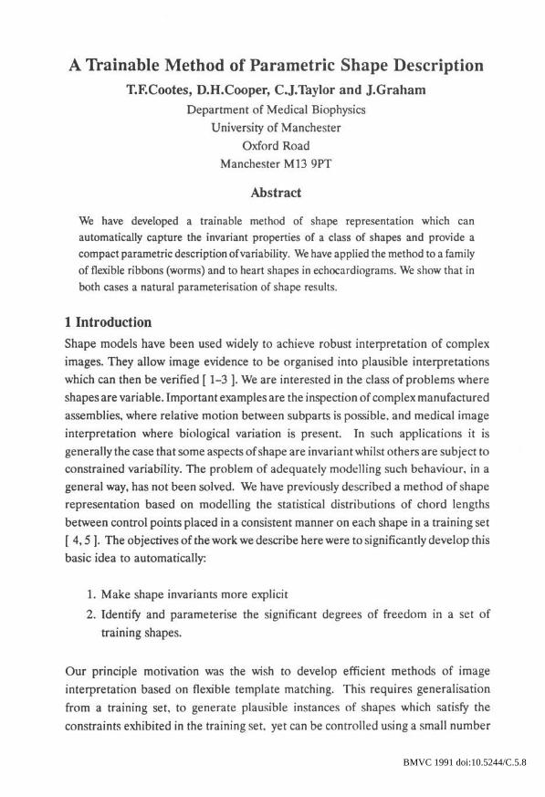
4.1 "Worms"

A set of 21 "worm" shapes, each described by 12 boundary points (Figures 1 and 2),

was used to train the system. The worms varied in length and axial curvature but

were of constant width. This example represents a challenging problem for the

method; the important invariant is an axial symmetry which we wish the system to

discover from the example shapes. At the same time we wish the parameterisation to

allow significant variations in length and curvature.

2 3 4Q O O

0 0 011 10

Figure 1. Labelling of 12 Point "worm"polygon used in training.

Figure 2. Examples of 12 point worms intraining set.

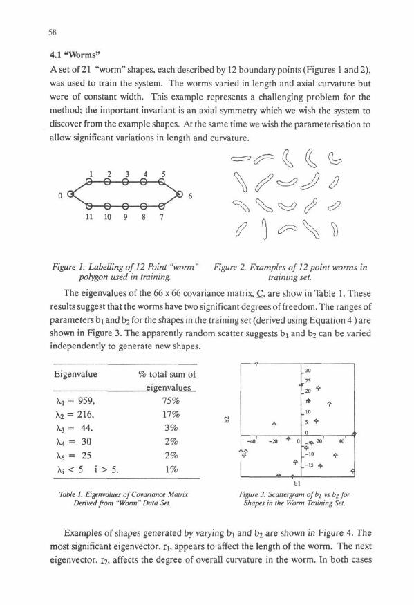
The eigenvalues of the 66 x 66 covariance matrix, £ , are show in Table 1. These

results suggest that the worms have two significant degrees of freedom. The ranges of

parameters bi and b2 for the shapes in the training set (derived using Equation 4 ) are

shown in Figure 3. The apparently random scatter suggests bi and b2 can be varied

independently to generate new shapes.

Eigenvalue

M = 959,

\ 2 = 216,

X3 = 44.

X4 = 30

X.5 = 25

Xi < 5 i > 5.

% total sum of

eigenvalues

75%

17%

3%

2%

2%1%

Table 1. Eigenvalues of Covariance MatrixDerived from "Worm" Data Set.

<2•?•

-401 -20' * 0

t

25

20

- * +10

5 +0 /

^ 2 0 40

. - 1 0 ^k

-15 ^.

bl

Figure 3. Scattergram ofbj vs b2 forShapes in the Worm Training Set.

Examples of shapes generated by varying bi and b2 are shown in Figure 4. The

most significant eigenvector, ii , appears to affect the length of the worm. The next

eigenvector, &, affects the degree of overall curvature in the worm. In both cases

59

axial symmetry is preserved. The third parameter determines the amount to whichthe ends of the worms curve in opposite directions, but its effects are small as therewere few examples of this in the training set.

Figure 4. The effects of varying the parameterscorresponding to the largest two eigenvalues.

4.2 Heart Data Set

A project currently being undertaken by Hill and Taylor [ 9 ] involves finding the

boundary of the left ventricle in echocardiograms, ultrasound images of the heart. A

'hand crafted' parameterised model of the boundary is matched to the image using a

Genetic Algorithm. We have investigated the possibility of constructing the model

automatically from a set of examples. A training set was generated by manually

drawing the heart boundary on each of 66 images (Figure 6). Each boundary was

represented by an 18-vertex polygon . Four control points were placed on each

boundary by hand, the 14 other points were equally spaced along the boundary

between the control points.

The eigenvalues of the covariance matrix derived from the shapes in the training

set are shown in Table 2. The ranges of parameters bj and b2 for the shapes in the

training set (derived using Equation 4 ) are shown in Figure 5.

60

Eigenvalue % total sum ofeigenvalues

\i = 24076\2 = 952\3 = 465X4 = 330\s = 209

91%4%2%1%1%

2 Eigenvalues of Covariance Matrix

Derived from 'Heart' Data Set.

-4 10 -300 -200^-100^ ^ 0 ^ 1 » 2Gp 300

••• •»•

Figure 5. Scattergram ofblvs b2 for Heart Shapes in

Training Set.

The results of varying the first four parameters are shown in Figure 7. Theparameter associated with the largest eigenvalue, bi, controls the scale of the shape.The second parameter, b2, seems to affect the width of the shape. The third andfourth parameters seem to affect the width and the form of the base of the shape,which corresponds to the opening and closing of the mitral valve in the heart.

Obi

Qa[

3D

u—>y

Q

DD

Do00

00

ft; = -JOO

nniU LJ Ib2 = -45

ftj = -45

ft4 = -30

QQQQQ

ft* ¥2 = 0 b2 = 45

r\ r\ r\ r\ r\JUUUU

bk43 = 0 b3 = 45

Figure 6. Examples from the TrainingSet of!8-Vertex Heart Shapes.

Figure 7. Effect of varying the para-meters associated with the fourlargest eigenvalues.

5 Discussion

The method has been applied to two cases and in both gives a parameterised modelof shape. The resulting models have both been used to find boundaries in noisyimages.

61

For some types of variability (eg rotation of one subpart around another) theassumption of linear dependence between chords does not hold. This leads tocorrelated b-vectors for members of the training set, so it is not reasonable to choosethe elements of the b-vectors independently when seeking to generate a newinstance of the model. We are looking at ways of dealing with this.

Although the examples given above are of shapes, it is the position of the pointswhich are modeled. These can represent vertices of polygons or the positions ofsubparts equally easily, allowing spatial relationships between parts to be modelled.

The method could be used to model the image variability due to small changes inviewpoint and lighting conditions in industrial inspection.

The choice of points in the training set is important. Each point must be in aposition which can be reproduced in each training shape. Choosing points can be away of using human expertise in the training phase, though it would be useful toautomate the procedure of positioning the points on training images as much aspossible.

6 Acknowledgements

This project is funded by SERC, under the IEATP initiative. (Project No. 3/2114).The authors would like to thank Andrew Hill & David Bailes for their help inpreparing the training set for the heart model.

7 References

[ 1 ] Chin R.T., Dyer C.R. Model-Based Recognition in Robot Vision. ComputingSurveys, Vol 18, No 1, 1986

[ 2 ] Grimson, W.E.L.,Object Recognition by Computer : The Role of GeometricConstraints. The MIT Press, Cambridge Massachusetts, 1990

[ 3 ] Cooper D.H., Bryson N., Taylor C.J. An Object Location Strategy using Shapeand Grey-level Models. Image and Vision Computing, Vol 7, No 1, pp 50-56,1989

[ 4 ] Taylor C.J. & Cooper D.H., Shape Verification using Belief Updating,Proceedings BMVC 1990

[ 5 ] Cooper D.H., Taylor C.J., Graham J. & Cootes T.F. Locating OverlappingFlexible Shapes Using Geometrical Constraints. (This Volume).

[ 6 ] Gower J.C. Euclidean Distance Geometry. Math. Sci., Vol.7, ppl-14 1982

[ 7 ] Fukunaga K. and Koontz W.L.G. Application of the Karhunen-LoeveExpansion to Feature Selection and Ordering. IEEE Trans, on Computers, Vol.C19, No.4, April 1970.

[ 8 ] Gill P., Murray W. and Wright M. Practical Optimisation. Academic Press Inc.,1981

[ 9 ] Hill A. and Taylor C.J. Model Based Image Interpretation Using GeneticAlgorithms. (This Volume)