University of Wollongong University of Wollongong

Research Online Research Online

University of Wollongong Thesis Collection 1954-2016 University of Wollongong Thesis Collections

1984

A three dimensional solution for a magneto-elastic vibration in a sphere A three dimensional solution for a magneto-elastic vibration in a sphere

Agus Kurniawan University of Wollongong

Follow this and additional works at: https://ro.uow.edu.au/theses

University of Wollongong University of Wollongong

Copyright Warning Copyright Warning

You may print or download ONE copy of this document for the purpose of your own research or study. The University

does not authorise you to copy, communicate or otherwise make available electronically to any other person any

copyright material contained on this site.

You are reminded of the following: This work is copyright. Apart from any use permitted under the Copyright Act

1968, no part of this work may be reproduced by any process, nor may any other exclusive right be exercised,

without the permission of the author. Copyright owners are entitled to take legal action against persons who infringe

their copyright. A reproduction of material that is protected by copyright may be a copyright infringement. A court

may impose penalties and award damages in relation to offences and infringements relating to copyright material.

Higher penalties may apply, and higher damages may be awarded, for offences and infringements involving the

conversion of material into digital or electronic form.

Unless otherwise indicated, the views expressed in this thesis are those of the author and do not necessarily Unless otherwise indicated, the views expressed in this thesis are those of the author and do not necessarily

represent the views of the University of Wollongong. represent the views of the University of Wollongong.

Recommended Citation Recommended Citation Kurniawan, Agus, A three dimensional solution for a magneto-elastic vibration in a sphere, Master of Engineering thesis, Department of Civil Engineering, University of Wollongong, 1984. https://ro.uow.edu.au/theses/2373

Research Online is the open access institutional repository for the University of Wollongong. For further information contact the UOW Library: research-pubs@uow.edu.au

A THREE DIMENSIONAL SOLUTION FOR A

MAGNETO-ELASTIC VIBRATION IN A SPHERE

by

AGUS KURNIAWAN

A thesis submitted in partial fulfilment of the requirements for the award of the

degree of

MASTER OF ENGINEERING

from

THE UNIVERSITY OF WOLLONGONG

UMÍVIRSITY Qr j W#LLONGONG j

W A R Y 1

Department of Civil Engineering

1984

ACKNOWLEDGEMENTS

I wish to thank Dr. A. Basu, of the School of Mechanical

Engineering (previously of the School of Civil Engineering), of the

University of Wollongong, for his support and guidance during the

writing of this thesis.

I am indebted to my parents, Mr. & Mrs. H. Kurniawan, for

their emotional and financial support during the whole of my

secondary and tertiary studies.

TABLE OF'CONTENTS

ACKNOWLEDGEMENTS

TABLE OF CONTENTS

PRINCIPAL SYMBOLS USED

Page

0 )

(ii)

(iii)

ABSTRACT

1. INTRODUCTION

2. BASIC EQUATIONS

3. STATEMENT OF THE PROBLEM AND ITS SOLUTIONS

4. GENERAL STATEMENT OF MAGNETO-ELASTODYNAMICS PROBLEM

5. CONCLUSION

1

2

ryj

8

14

23

REFERENCES 24

APPENDIX A NUMERICAL TABLES FOR FIG. 4.2, 4.3, 4.4 25%

APPENDIX B FUNDAMENTALS OF MAGNETO-ELASTIC RELATIONS 27

APPENDIX C MATHEMATICAL FUNCTION 33

APPENDIX D MATHEMATICAL CALCULATIONS 37

PRINCIPAL SYMBOLS USED

a radius of sphere

B magnetic induction vector

Cl a longitudinal wave velocity [(x+2y)/p]^

C; a transverse wave velocity (y/p)^

S' electric displacement vector

6ij

t

strain tensor

electric field vector

fn (r)

ft

function of r

magnetic field vector

Ho

ft

character!’Stic external magnetic field

conduction current density vector

J _ ( k nr) n + V n ‘

the spherical Bessel function '

"i unit normal in i direction

P n (.COS0) Legendre function of degree ‘n 1

r hHartman's Number

U.1 unknown reaction on the boundaries

U, V, w displacements in x, y, z directions respectively in Cartesian co-ordinates

V

V V % displacements in r, e, <j> directions respectively in spherical polar co-ordinates

won the nth circular frequency in free vibration

Xi body force

6.1 j

X

Kronecker symbols

Lame' constant

uemagnetic permeability

(iv)

Ti j '

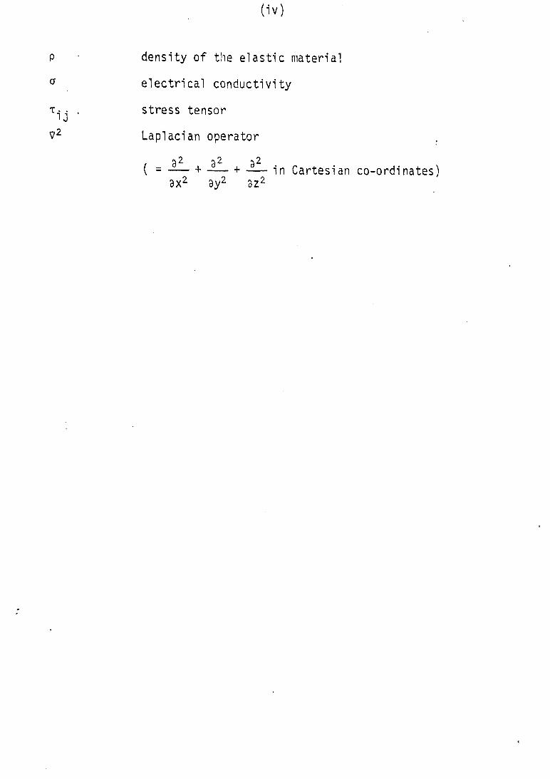
density of the elastic material

electrical conductivity

stress tensor

Laplacian operator

( = l 2 ■ a2

3X-+ --- + ---- in Cartesian co-ordinates)

3y- 3Z‘

2

ABSTRACT

ABSTRACT

A three dimensional solution for a magneto-elastic vibration

in a sphere is considered. The normal mode method has been applied

to free vibrations, and the Airy stress-function's approach gives

solutions for the differential equations of motion. The response of

the system due to forced vibrations is obtained by developing the

external forces into linear combinations of all the normal modal

functions. Numerical solutions for radial and transverse displace­

ments have thus been obtained. Furthermore, graphical solutions for

axisymmetric displacement have also been provided for different modes

of free vibration.

In the above-suggested analysis, the coupling of electro­

magnetic and elastic waves is considered from the standpoint of linear

elasticity and linearized electro-magnetic theory. The investigation

of this coupling effect predictably shows that the effect of the

magnetic field is to lower the amplitude of the elastic vibration.

INTRODUCTION

- 2 -

1. INTRODUCTION

The theories of magneto-elasticity are concerned with the

interacting effects of an externally-applied magnetic field on the

elastic deformations of a solid body.

These theories have been rapidly developed in recent years

because of the possibilities of their extensive practical applications

in such, diverse subjects as geophysics, optics, acoustics, damping •

acoustic waves in magnetic fields . Although there has

been some progress in the study of magneto-elasticity [6-17], the

development of effective methods of solution for the general mixed

initial and boundary value problems in magneto-elastodynami.es remains

a challenge.

A complete and systematic mathematical formulation for mixed

initial and boundary value problems in magneto-elastodynamics (MED)

with mixed boundary conditions has been developed and applied success­

fully to two-dimensional problems [18-19], As an application to

three-dimensional problems, this thesis ' considers a three­

dimensional solution for a magneto-elastic vibration in a sphere; and

also to investigate some of the dynamic interactions that can occur

between electro-magnetic and elastic fields in a homogeneous isotropic

solid sphere.

tt will be. seen in Section 2 that the electro-magnetic field

generated by the application of the primary magnetic force is described

by Maxwell equations and the elastic field by Hooka's law equations.i

The theory is essentially a combination of infinitesimal

elasticity and a linearized electro-magnetic theory. The interaction

effects considered consist of the Lorentz body force (J x B) and the

- 3 -

-*■ ->• ->generalised Ohm's Law J = a(E + -— ■ x B).

3t

A general theory [2] for magneto-elastic bodies was presented

for solving problems of magneto-elastodynamics with mixed boundary

conditions.

An elastic spherical body is considered in vibrations under

mechanical load and large magnetic fields. The boundary value problem

requires careful consideration of electro-magnetic elastic boundary

conditions. Based on. the Betti's reciprocal theorem, a formulation of

the boundary value problem in integral equations form Eq. (4.12) is

given, using Green's functions.

As a fundamental system, the sphere is chosen to be entirely

fixed and with this system, the Green's functions are found. When the

field point lies on the boundary contour, a boundary formula is

obtained which expresses a relation between boundary displacements and

corresponding boundary tractions.

Since either of these boundary quantities, in principle,

determines the other, the formula provides a constraint between them,

which generates a set of simultaneous integral equations from suitable

boundary data. •

From observation, on some part of the surface (Sx), the

displacements: are known while the surface forces are unknown, and on

the remaining part of the surface (S2), the loadings are known while

the displacement functions are unknown. Thus the possibility of

choosing unknown functions in two ways leads to two ways of solving

the problems of magneto-elastodynamics. Within this thesis, the ,

unknown functions of the problem are taken to be the displacements

u of the surface $2.

- 4 -

The field equation governed by Eq. (2.1) and the constitu­

tive equation governed by Eq. (2,3) are linearized by assuming that. -»•

the magnetic field, H, is composed of a large static field, H , plus

a small fluctuating field, h(H = Hq + h). The graphical solution for

axisymmetric displacement have been provided for different modes of

free vibration.

BASIC EQUATIONS

- 5 -

2. BASIC EQUATIONS

Consider a conductive, homogeneous, and isotropic*

elastic medium, in motion, in the presence' of a constant magnetic

field.

The electromagnetic vectors, E, H, D,and B satisfy

Maxwell's equations [4]:

■ -ncurl H = J + , di v B = 0

-hr. D +

curl E = - ~ r , d i v D = 0at ’ ( 2 . 1 )

and the constitutive equations [4]:

B = ueH D = eE

J = a(E + X B)

( 2 . 2 )

(2.3)

where J is the current density, and e are the magnetic ande

electric permeabilities, o is the electrical conductivity.

The stress-strain relation in an elastic solid is [l]:

t . . = 2u e • • + Xe<$. . (2.4)

where:.

e ij = ^ i ’j + uj,i>’ e = div u (2.5) 1

•» 6

The equation of motion in component form is:

®2ui ^Tik **■ p — 2“ = + (J x B), + p X.

3t axk 1 1(2 .6 )

where p is the density of the elastic material and X, is the body

force.

form:

If (2.4) and (.2.5) are used, the equation (.2.6) takes the

32U 9f , . +p— _ b UVZU + (X + u), grad div u + (J x B) + p X (2.7)atz '

Using the equations (2,1) - (2.3), the equation (2.7) can be

re-written in the form:

a£u

at2= c22ÿ2u + (cx2 - c22 ) grad'div u + Rw J x H + pX

where : Ru H 2 He o

(2 .8)

H , a Hartman's number

V »X+2yi , a longitudinal wave velocity

Ç 2 = H.¿ P

H

a transverse wave velocity

a constant.external magnetic field

- 7 -

Generally, the induced magnetic field is small, compared to

the constant applied external magnetic field, so that its higher order

powers can be neglected. Also, the elastic displacements are infini­

tesimal and the displacement currents are negligible compared to the

conductivity currents. The general form of the linearized magneto­

elastic equation for a perfectly homogeneous isotropic body is:

lii s c22v2u + (cj.2 - c22) grad div u312 **■

+ [curl curl (u* x H)] x H + X (.2.9)

STATEMENT OF THE PROBLEM

AND ITS SOLUTION

- 3 -

3. STATEMENT OF THE PROBLEM AMD ITS SOLUTION

Consider.a conducting, isotropic, and homogeneous solid

sphere of radius 'a1 (Fig, 3,1), On one part, Sj, of the surface the

displacements are given, and on the remaining part, S2 , the loadings

are prescribed.

Fig. 3,1: Fig, 3.2:

If r, 6, 4 are spherical polar co-ordinates and up, uQ, u^

are the displacements in the directions of r, 8, <j> respectively (Fig.

3.2), then for rotational symmetry, the displacement u^, as well as the

stresses t t _. vanish. The radial and transverse displacements u ro o(j> r

and uQ respectively are independent of <j>.

Using the fact that H. = Hq £ , the magneto-elastodynamics

equations of motion (2.9) can be written in the form:*

(Cj2 + Rm h 2) V2$ - — = 0at2

in the absence of body forces,

where: u = — and u = ~ —" r ar Q rse

i2 = i _ i _ (r2— ) + ---- (sine )*2 ar ar r2 sine ae a6

(3.1)

(3.2)

(3.3)

* For details, see Appendix B.

_ 0 _

For harmonic solution of (3.1), we take:

00 ia)nnt$ = l fnCr) Pn(.cose) e n (3.4)

n=0

where: f n(r) is a function of r only,

Pn(cose) is a Legendre function of degree 1n19 and

cu on is the nth circular frequency.

Substituting Eqn. (3.4) into Eqn. (3.1), we obtain:

fn(r) Jn ^ (-knr)

/r(3.5)

where Jn+^ (kn^)is the spherical Bessel function and

kn

on

Ci2 + R. H 2 o

(3.6)

If $ is known, the expressions for the displacements, u^ and uQ ,

under forced vibrations can easily be found.

Forced Motion:

Defining:

Liur = c22v2up + (cj2 c2 2 ) f ­z ' ar — — (r2u ) 2 3r v r' rz

+ RH Ho2 ~ ÏF (r2 ^ > + — — ïë- (sin0^r2 ar 3r r2 sine 30 30

1-2 = ( Ci2 - C22 ) TT 1 aar jr sine■ae v~e

' /

(ua sine)

Leu. = (C!2 - c2 2) ±1 ar ae — T - (r2u )

.2 3r r;

- 10 -

+ Ru H 2 H o

L-iur + L2u q + Xr

L3u + L,un + X J r H 0 e

( q 2 - c22) J ___ 1le (ue S1ne)rse r sine

i i fr2Sue r 2 Sr 1 3r ) +

1 a 3u„ 39 (Sln8résine

e re-written as:

32Ur

312

32Ue

(3.7)

3t2(3.8)

Green's functions due to a unit harmonic concentrated load in the

radial direction at a point (r ,e ) can be found to be:

• ô(r-r') 0(0-0*')t-l9rr + L2grQ + ■ ; = -0)2g

r2 sine rr

L3grr + Li*gr0 + o = -w2gre (3.9)

Solutions to (3.9) are assumed in the form of modal functions

grr = I U (r) Tn pn(cos8)e1u4>t

'i»ft " I Un > ) Tnre l ' en* ' ' n rn (3.10)

where u ^ , u- are the nth modal functions obtained in the free vibra- rn 0n

tions. This method is given in reference 3] .

The given loading functions in terms of urn>uQn are expanded

as:

Xr ‘ ^ n ur n W

xe " ? % uen(r) (3.11)

- 11 -

The functions X and Xfl are given by, after substituting (3,10)

into (3,9):

ö(r-r') (2n+l) p (cosejy - _____ o n oV - •o

r- 2(3.12)

xe = 0

1(using the fact / pR (x) pm (x) dx 0 if n f m and if n = m)

•The substitution of (3.10) and (3.11) into (3.9) yields:

"V"lUrn+ T L2uQ + q =

n ^ 0n ^n -u2T u n rn

V 3Urn+ T Luu„ + q = n H en Mn -w 2T un

n en(3.13)

u n and u Qn satisfy the homogeneous equations:

Liu^ + Lo u q1 rn ön

■Oi 2uon rn

L3urn + U u en•03 Uon en

(3.14)

the form:

The substitution of (3.14) into (3.13) can be written in

{T (w^-u) ^) + q } u = 0 nv on' Mn rn

{T (io -oj ^) + q } u = 0 n^ on' Mn en(3.15)

- 12 -

These equations (3.15) will be satisfied if:

T (w2-o> 2 ) + q = 0n^ on' Hn

Note the orthogonality relation [3]

{ [Xr urm + Xe u8m] 4*r2dr = l % V <urn ura + o n o

where integration is over the whole sphere.

Substituting Eqn. (3.12) into Eqn. (3.17):

a <S(r-r ) (2n+l) .p (cose )f — u • 4Trr2dr

2 rn

a

- % f [ % 2 + uen ] ‘ 4irr2dr

= q / 2 ,

where: % 2 = S 4*n-r2 [u_2 + uQ 21 dr is called the scale rn on J

or: 2*tt(2n+l) u ^ ( r ) P (cose ) = q i2' ' rn o n o n

or:2ir(2n+l) urn(rQ ) pn(cos6Q )

_

Substituting (3.18) into (3,16):

T2Tr(2n+l) urn(rQ ) Pn(coseQ )

A2 (0) 2 -Ü32); on J

(3.16)

uen uem>]4irp2dr

(3.17)

factor,

(3.18)

(3.19)

- 13 -

Hence, the Green's functions, given by (3,10), can be re-written

as follows:

u (r ) u ( r ) a - r rnw o ; rnv ;yrr "" l

n A2(w0n2-w2)• 2ïï(2n+l) pn(cos0Q ) Pecóse) eiüít

r 0P urn(rn) üfin(r) ■ *1 T;---:— “ — ♦ 2tt( 2n+l) P (COS0 _) P_(cos0) e1ujt

izU on2- ^ ) n' wo' n

( 3 . 2 0 )

If a unit harmonic concentrated load is applied at a point

(r0 »a0)> Para^ e to ^-direction, and the same procedure as above is

followed, the following relationships can be obtained:

u (r ) u (r) ." l Æ - 9-— - ------2ir(2n+l) P (cose ) Picóse) elut

n *2(<oon2V ) n 0 n

ga0Ô

» l V ^ o L V ^ , . .2ir(2n+l) P (coseJ P (cose) eiut n *2 U on2-u2) n 0 n

(3 .21 )

As all the components of Green's functions are known, they

can be used to solve problems where the boundary conditions are exactly

specified, •

GENERAL STATEMENT OF MAGNETO-ELASTODYNAMICS PROBLEM

- 14 -

4. GENERAL STATEMENT OF MAGNETO-ELASTODVNAMICS PROBLEM

Consider a simply-connected elastic body with region B and

a surface, S, consisting of two surfaces, Sx and S2 , intersecting

along a curve,a(Fig. 4.1).

a

Fig.4,1:

Inside the body, there act body forces t per unit volume,

on the surface S2 external forces q per unit area, and on the surface

Si, the displacements u are given.

Based on the general reciprocal theorem of Betti, a formu­

lation of the boundary value problem is given, using Green's function.

This theorem [1] and [20] has,' for. dynamic problems , the form :

t•

rf[10

Jjj(Xi(x,T )u-(x, t-T) - Xt(x,t-T)u.(x,t)} dv

riqi(x,T )u.(x,t-t) - q((x,t-x)u. (x ,t )} ds

(S)

iu.(x,T)ut(x,t-t) - uC(x,t-x)u^(x,t)} dv | dx = 0

(B)

(4.1)

- 15 -

where X -, denote body and surface forces respectively, which

produce in the body the displacements u^, while X:j and q? belong to

the other system of forces producing the displacements u^. It is

observed that, on the surface, Sx the displacements are known, while

the surface forces are unknown on this surface. On the surface S2

the loading q* is known, while the function u- is unknown. Hence,

in solving problems with mixed boundary conditions, the unknown function

c^n be assumed as either q^onSj, or u. on S2 ‘, calling them the first

variant of solution or the second variant of solution, respectively. '

The displacements u.. and the loadings q. are related by the

relation:

L tup . = qn- = uCih j + Uj ^ n . + An. div u, (4.2)

where n, and n. denote the components of the unit normal vector of the* J

surface S. .

The equation (2.9) can be re-written in the operator form:

. Du + 1 = 0, (4.3)

where the operator D = c^72 + (cf - c£) grad div + x constant

coefficients.

In this Investigation, the unknown functions of the problem

are assumed to be the displacements u. of the surface $2. As a

fundamental system, the elastic body is chosen to be entirely fixed

on and S2 , and it is also assumed that the Green's function '

$ =-.19^3 (i,k s 1,2,3) satisfy differential equations (2.9):

- 16 -

at2c£v2g + (c? - c£) grad div g

+ Rh [curl curl (g x H] x H + 6(x - x") 6(t) (4.4)

and the boundary conditions:

g(S,x",t) = 0 on Si and S2 (4.5)

and the initial conditions:

g(x,fr,o) = a ,x% o ) = 0

In operator form, the equation (4.4) can be re-written as:

°1 j ^9jk(x,x ',t)] + $(x - X ') 6(t)6ik = 0 (4.6)

the operator D = [D. .] (i,j = 1,2,3) is defined in (4.3).* J

After carrying out the Laplace transformation and using the

initial conditions u.(x,o) = U.(x,o) = 0, the equation (4.1) can be

expressed in the form:

' r r

J J.(B)

- X?u.j )dv +* f

J,(S)

q-u^ds = 0 (4.7)

From (4.3)i X,= -»O-.u. and from (4.2), q, = Uu.3, the equation (4.7)I I J J

can be written in the form:

JJJ(B)

[-ufD, .(u.) + u.O. .(ut)]dv + (utL(u.) - u,L(u:p]ds-= 0» lJ J > > J J J J J 1 1 1 1

(S)(4'.8)

- 17 -

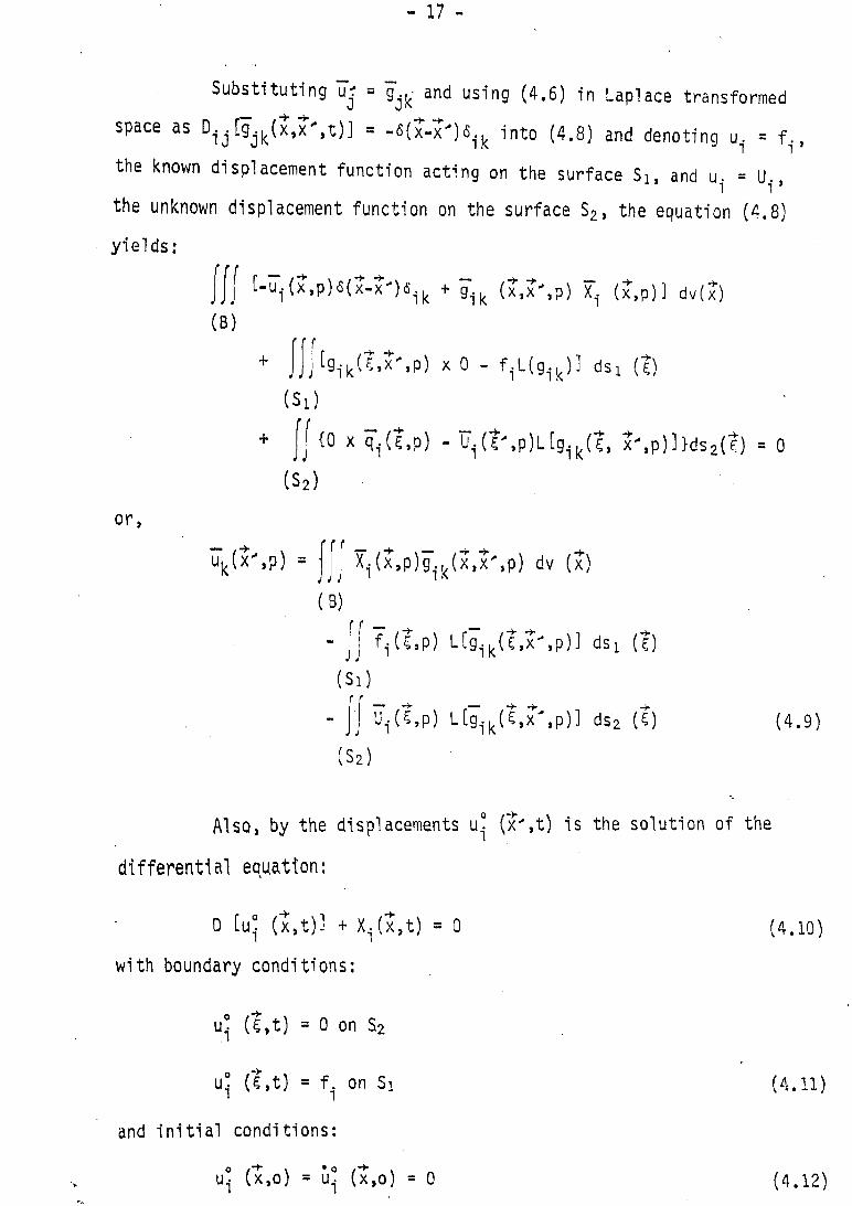
Substituting u> = g^- and using (4.6) in Laplace transformed

space as D . tgjj<(x>x'*,t)] = -<s(x-x^)<s^ into (4.8) and denoting u = f..,

the known displacement function acting on the surface Si, and u. = U .,

the unknown displacement function on the surface S2 , the equation (4.8)

yields:

|{ + g . k (iT.X'.p) X. (x,p) ] dv(x)

(B)•

J JJ (g1k(f,x',p) x 0 - fiL(g1k)] dsi (1)

( 5 1 )

r

J.(52 )

(0 X q.(?,p) - U.(t',p)L[gik(t, x',p)]}ds2(t) = 0

or,

J

H I Xi(x,p)gik(x,x',p) dv (x)

(B)

- jj fi(1’,p) L(gik(t,x',p)] dsi {t)

( S i )' f

- JU^S.p) L[gik(t,x',p)] ds2 (5)

(Sz)

(4.9)

Also, by the displacements ul (x-,t) is the solution of the

differential equation:

• D (u!j (x,t)l + X^x.t) = 0 (4.10)

with boundary conditions: ,

ui (l,t) = 0 on S2 .

ul (T,t) = f. on Si (4.11)

and initial conditions:

ul (x,o) = 0° (x,o) - 0 (4.12)

- 18 -

Now apply Betti's reciprocal theorem (4.7) to the function

ui and 9ik*

Introducing into (4.8), the relations:

— o^ = U., D[Ui(x,p)] = -X.

ui = 9i k ’ D ^9i k- ' = Sii k (4.13)

and i.j 5 o on S2, L(ITt) = o, on Si

ui = f.. on Si, L(u?) = qi , on S2

9ik = 0 Si and S2, (4.14)

the equation (4.8) yields:

■f •

J J.(B)

[- Ü! x 4(x-x')«ik + gik X Xi] dv

(0 - f^L (gik)] ds

(SO

(S2)

[0 - 0 x L(gik)] ds2 = 0

or u! (x'.p) =J

(B)

X^x.p) gik(x,x',p) dv(x)

,-v ->■f ^(t.p) L[g1k((,x',p)] dst(C)

(Si)

(4.15)

The combination of equations (4.9) and (4.15) can be written:

ï ï k ( x ' , p ) = ï ï £ ( x ' , P ) - j Ï Ï ^ ç . p ) L [ ? i k ( t , x ' , p ) ] ds2 ( I )

(S2) ' (4.15)

- 19 -

where:

For a spherical case, the Equation (4.16) reduces to:

= ak(V eo*ti , xuiCa .t)LlgikJdS2(a) (4.17) . S2(a)

V w 1 = V 9ikXidV ‘ c / ,flL-f9lk3dsiia>k s^aj

L u. = y (u • . + u . .) n. + xn. div1 1 > j j »1 j I (4.18)

Here Sx is the surface where the displacements are given, and S2 is

the surface where the loads are specified. Since all the quantities

^i'^ik’ anc* fi ln are known, the displacements u^ in the funda­

mental system are known. The unknown reactions, U^, in (.4.17) can be

found from the boundary conditions on S2 . •

The similar technique is used by Basu [ 21J and £ 22'"] in two dimensional cases.

FREE VIBRATION : ‘

When the relation (3.4) is used in (3.2), 4'he displacements

Up and uQ can be re-written- as:

00 iu t ioj. tU„ = l f'(r) P (cose) e n = U e on r n=0 n n r

00 f (r) . „ _ . „1 -41 P;;(cose) e on = u.e on0 n=0 r "

i w _ t i to t

8' (4.19)

where: » ffj(r) illdr

Pn(cos0) is a Legendre's function, and

d P

Pn (cos0) = 1 r (4a20)

The graphs for the radial displacement are drawn for different

modes in harmonic vibrations. v •

- 02-

- 21-

lip VS

Tirsi Mode, oj- Vibrai* on C ^ - O

- 22-

CONCLUSION

- 23 -

5. CONCLUSION

The graphs for the amplitudes U . U * of the displacements u *r o r

ue have been drawn for different modes (Cn = 0 ,1,2) of free vibrations.

The differences in the solutions portrayed graphically in

Figures 2 , 3 and 4. between the elastic and the magneto-elastic cases

are highly predictable, as the effect of the magnetic field is to

lower the amplitude of the vibrations of a vibrating homogeneous solid.

For the magnetic field to become significant, it would be necessary to

have an elastic material which is a perfect conductor, non-ferro

magnetic and mechanically soft,e.g. a perfectly conducting rubber or

soft plastic. The analysis of magneto-elastic waves has applications

in geophysical, optics, and acoustics problems. This theory can be

extended to include thermal fields, as would be the case in the theory\

of magneto-thermoelasttctty.

It is assumed that the medium satisfies £oHe0 - whioh

.leads to the assumption that, in this medium, the speed of light

approaches its value in vacuum. In the above equations the density of

the free charges is neglected , pg = 0 . Furthermore, a » 6 and y.Q

are considered to be constants, that is, the medium is homogenous from

the standpoint of its behaviour in the magnetic field.

r

REFERENCES

- 24 -

REFERENCES

[1] W. Nowacki, Mixed boundary value problems of elasto-dynamics, Proc. Vibr. Probl.j 5, 3,-(1964), 210-217.

[2] A Basu, An integral equation approach to mixed boundaryvalue problems of magneto-elasto dynamics, Proo. of Ind. So. Congressj January 1979, 1-10.

[3] Yu Chen, Vibrations: Theoretical methods. Reading,Massachusetts: Addison-Wesley Publ. Co., Inc., 1966.

U] G. Pari a, Magneto-elasticity and magneto-thermo-el asticity,Advances in Applied Mechanicsj Vol.10, 1, (1967), 73-112.

[5] G.N. Watson, Treatise on the Theory of Bessel Function(2nd ed.), Cambridge: Cambridge University Press, 1958.

[6 ] J.W. Dunkin and A.C. Eringen, Int. Jour. Engng, Sci.. 1,1963 ,.461-495.

[71 S. Kaliski, Proc. Vibr. Probl.j 3, 1962 , 225-234 .

[8] I, Abubakar, Appl. Sci. Res, B.j 12, 1965 > 81-90 .

[9] S. Kaliski, Proc, Vibr. Probl.j 1, I960 , 63-67 .

[10] S. Kaliski, Arch. Aicch, StostJ 12, 1960 , 229-234 .

[11] S. Kaliski, Arch. Afech, Stos.j 15, 1963 , 197-208 .

[12] R. Kumar, Proc. Vibr. Probl.j 3, 1967% 273-278 .

[13] R. Kumar, Proc. Vibr. Probl.j 8, 1967 , 369-379 .

[14] Ya S. Uflyand, J. Appl. Math. Mech.j 27,1964 , 1135-1142 .

[15] E.S. Suhubi, Int, J. Engng. Sci.j 2, 1964 , 441-450 .

[16] E.S. Suhubi, Int. J. Engng. Sci.j 2, 1965 , 509-517 .

[17] G. Pari.a, Proc. Cambr. Phil. Soc. A.3 58, 1962 , 527-531 .

[18] A. Basu, Acta. Phys. Hung.j 43, 1977 , 81-91 .

[19] A. Basu, «Joum. Technical Phys.j 18, 1978 , 1 & 151-160 .

[20] W. Nowacki, Proc. Vibr. Probl.j 3, 1964 , 161-177 .

[21] A. Basu, Acta. Phys. Hung.j 45, 1978 , 1 5-25 . .

[22] A. Basu, Joum. Math. Phys. Sci.j 12, 1978 , 589-598 .

APPENDIX A

NUMERICAL TABLES FOR FIG. 4.2, 4.3, 4.4

s

T A B L E A . 1

N U M E R I C A L T A B L E F O R F I G . 4 . 2 , 4 . 3 , 4 . 4

ur

n = 0 n = l n = 2

r/a E l a s t i cM a g n e t o - El a s t i c

E l a s t i c M a g n e t o ­E l a s t i c

E l a s t i cM a g n e t o ­E l a s t i c

0 Singular Point Singular Point 0.14514 0.13977 Large Number Large number

1 -0.34581 -0.32907 0.16285 0.1606 4 4.57812 4.39145

2 -0.50454 -0.47589 ’ -0.05208 -0.04315 0.72763 0.69201

3 -0.38537 -0.32935 -0.15336 -0.14459 0.21426 0.21216

4 -0.16179 -0.12687 -0.12996 -0.12209 -0.0259 7 0.02073

5 0.13167 0.10389 -0.03193 -0.03239 -0.13936 -0.11872

6 0.19149 0.18333 0.05921 0.04922 -0.12496 -0.11970

7 0.09871 0 . 09303 0.06969 0.06565 -0.04877 -0.04233

8 -0.06483 -0.04676 0,03131 0.02897 0.06367 0.04436

9 -0.12633 -0.11617 -0.03373 -0.02317 0.08472 0.07802

10 -0.08838 -0.08574 -0.04848 -0.04725 0.04506 0.04486

irotn

7

- 26 -

TABLE Ao2

n=l

r/a Elastic Magneto- El astic

1 -0.0566 -0.054845

2 -0.040211 -0.039644

3 -0.02136 -0.020975

4 -4.191 X 10" 3 -5.286 X 10-3

5 4.1887 X 10" 3 3.4633 X 10" 3

6 5.097 X 10‘ 3 5.093 X 10' 3

7 2.8925 X 10-3 2.45304 X 10" 3

8 -1.288 X 10-3 -7.659 X IO'“

9 -2.225 X 10' 3 -6.4866 X IO-4

10 -1.582 X 10‘ 3 -1.429 X 10' 3

APPENDIX B

FUNDAMENTALS OF MAGNETO-ELASTIC RELATIONS

- 27 -

APPENDIX B FUNDAMENTALS OF MAGNETO-ELASTIC RELATIONS

The three dimensional magneto-elastic equations for a

perfect conducting homogeneous isotropic body in vector form:

32U~ = c22v 2u + (c 12-c22) grad div u

at2 0 0

+ R^fcurl curl(uQ x H) x H] + XQ

u x H o

er ee %

y UQ Uj. r 0

Hr He H*

= H H* - u* He )er - (ur H* ' % Hr)ee

+ ur 8 " ue <)>

where:

= A e r r

= A

Ar = ^ H,<p

A8 = -«V H.

%= 0

curl curl (u0 X = V xy x(uQ x H) x H

-r ->V x v x (u x H) x H = v x v x A x H

V X 7 X A X H = [v (v*A) - v2A] X H. e,4> ♦

= [grad d iv A - v 2A] x H, e ,«P i1

-+ ->■div A = V*A = 1 3 f r 2A Ì +

2 3r ? rs ine 90 v ‘e ( A ,'in9Ì+ ^A<lA‘sin9] + r s T n ä l T

grad div A = v«(v«A) = arA A (r2/\ \ +_ L

2 ar v T) rsinô 30 ' “ 0

+ — —r 36-L A. (r2n \ + .... 1 _„2 3r ArJ + rsine 30- (Aesin0) + F i f e e ^

1 arsm© a<j>

A A (r2^ \ + _ L2 ar v T rs in0 aa v 09 (AQsin0) + ^_____ 9A¿

rsin0 3(j)

'!-A ■ ( ^ ) * - J - Á L (s1„eM , * _ ± _ Ü Mr ¿s in 20 9<j>¿,2 9r ar r 2sin0 30

Then,

[grad div A - V*A] = Aar

A A (r2 a } + -1. A2 3r VT rs ina 90 (A0sin0)

I Ar a© 2 ar ( r2Ar) + r s i ne 30 ( Aes in e )

1 9rs in0 9(j)

1 a 1 32 ar ( ^ A p ) + rsin0 90 v,,0(A .s in0 )

•+e

— v r (r2|£) - — — |e (sine f£) r 2 3r 3r r 2sine 36 39

fD i

[grad div A - V2A] x -

d_ar

- (A s i n e )r s i n e ae e

1 _a_

r ae

e

T ^ (r2A- > + 1r s i n e ae v e(A„sine) 1 a

r s i n e a<f>

i_ JL ( r2?-Ar\ o ar v * a r J

r 2 si ne

a / - aAp\

36 (s1n0T f )r 2 si ne

1 Ji_ r s i n e ae

0 0 0

1

(A.si ne) + 0D

roUD

- 30 -

Therefore the values of vectors u in directions of r and 6

are:x 2 o u

0 f2 = c22V2:ur + (C!2-C22) grad div ur + RH [curl curl (ujcH) x H] + X

.2ç) U

0 1C22V2Ur + (Cl2-C22) £ 1 3 1 3

T 37 ( r 2 u r } + 7 S Î W se ( ues i n 6 )

+ RH F T e (r* V + H P m (Aesin9)} - “ '(r2l T )r r

1 a 3A -»■(sine-— ) + Xro . 36 ' ----- 36

r2sine

à u ~r ->•e

c)t2

= c22V2uQ+ (Cl2-C22) grad div uQ + [curl curl (u0 xH) x H] + X

^ U® = C22V2Ue + (Cx2-C22) i - 3-0 t

r 301 1L ( p 2y ) + J:- - L. ( y c i n 0 )

* 3r r ; rsin0 30 1 e5 ;

- RH3 , 1 3 1 3ar ^ a ? ( r 2 V + F 5 Ï F ? ï ê ( A es i n e ) } “ “ “ ( r2^ " >

aAJL -L (r 2— r>„2 3r v 3r

1 aaA

rasineae W " * " )

H + Xo (j) 0

Substitute the values of A r and AQ with UQH and

resp ective ly. Therefore:

32u

I T 2£ - C 2 2 7 2 U r + ( C l 2- C 2 2 ) ± 1— L. (n2u ) + — v-----— (u sine)

2 3r 1 V rsine se e ;

+ RH i _ i . ,_ L _ L ( r 2u„H,) + ^TTTTS-Tû (- u„ Ha s in e )}r ae *"r 2 ar 0 rsin 0 30 v r ^

- 31 -

- W - ^ w (-s1n> i f V , ) H. + X„ p r

32ue3t2

= c22v 2 u . + (c i2- c22 ) r 80 i l F (r2ur) + H ® ¥ (uesin0)

- RH 3 {— (r2 u H ) + — t--- —-2 e V rsine as3r \_9 "e'V ' rsine aa ^"‘ur n®^^ X JL (r2_L u h )

„2 9r ar e V

— -— ^ (sine-^r u H ) r2sine 30 30 0 ♦ V X8

As a preliminary to the analysis of the forced vibration,

first consider the free harmonic vibration, i.e. X = 0. By

replacing:

Aar <»*&>

1

r2sin0J Lae (sine^)

with v2 u and.u = and u = , where $ is a stress function,r a r a r d a

the equations become:

a3$

a t 2 ar- (C22+ RHV )V2 (Ci2*C22) 3ar ar

X JL (r2^2 ar A 3r;

1 a / • n 3$ \ rsine ae rae; + r u h a 2!^ I s- I f ^r2^H <r|r 30 r 2

1 3r s i n e 38

. 30,s i n e - }

33*

rst236(C22+RuH*2)V2— + (Cl3-C23)WH‘> rae rae

X JL (r2l$.)r 2 3r v ar;

- 32 -

1 3 / • 3 $ \+ rsine ae- s1ner3F^ r h V

JL /_L -1- ( r2 9 $ \3r o 3r w r39 ' .r

_ 1 _ JL fsine— irsine 36 ^ mo3r'

Also (r2|fr) + ^ (sin0F 3? ) "

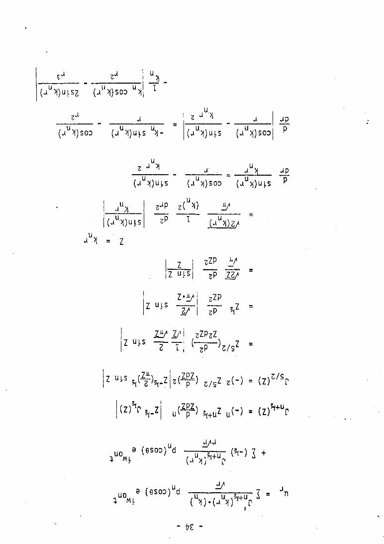
By substituting the value of $ = f (r) Pn (cos e'

,, ( k n r)

fn(r) = - 2 3 - 2 - n /r

P (cos e) is the Legendre function

The relation:

1 JL (r2Ü _ ) -------1------L (sine— ) = 0r1 3r K r30y r sine 36 ' °3r'

gives the roots of k .

, where

APPENDIX C

MATHEMATICAL FUNCTIONS

- 33 -

APPENDIX C MATHEMATICAL FUNCTIONS

F o l l o w i n g C 53 t h e f o l l o w i n g r e s u l t s c an be u s e d :

i—»iiCDtnOoo

O- when n =0

p ^ c o s e ) = c o s e when n = l

P 2 ( c o s e ) = ^ ( 3c o s 2e + l ) when n =2

When n=0:

V knr) sin(knr)

K n c o s (k n r ) , S l n ^ n r --------------------- --- -----------------

/r r / r

When n=l:

J3/2^k nr^

j 3;2 m

- ! ^ \ s" M k nt')

s i n ( k r )

~ T j F - costk nr>

= - h ( r r i ~ r ) h 1w j ' 7 7 2

+ ( 2 1

W } 7*

<'7 V T P i )' n

s i n ( k r )

— 7 ----------c o s ( k n r )

k c o s ( k r ) s i n ( k r )

n n n— + k s i n ( k r )2 n v n ;k r

n ( k r ) ' n '

”s i n ( k r ) '

2 r k r c c M n j nL

k c o s ( k r ) s i n ( k r ) n n v "

•k r n

— - — + k s i n ( K r ) k r 2 n v n

n

= ( *- - yL VV *■tt( knr)

3 s i n ( kn r ) c o s t e r )

k nr 2

+ c o s ( k r ) + k s i n t e r )

= I W V 1 ciwon11 dPn

r / rde

(UU >1) U LS2 (UU >i) SOD %

(UU >í) SOD (aU >l)ULS u>|

u.z ** ^( U U >i ) U L S (aU >l)SOD

jpp

uz J >1 J >j jp

(jU>i)ULS (jU>l)SOD (uU >i) U LS P

(j >j)ULS

z^P z( y) Ü/

3P I i ± 2 ù Z /

¿ >1 = Z

Z ULS

zZP V

“T P 1 1 7

Z ulsz - y

2/

zZP

zP1 =

Z ULSI V I/1~ T

32P3Z

>!/SZ ■

Z ^(Çls.-ZZPZ

Z ^ ) S/9Z «(“ ) = (Z)S/SC

(Z) T «,_Z u ( ^ ) u(-) - ( z r ur*f+U,

u ji/1“*

, < (eso” d 1™ (ir) 5 *

8 («t<o)“d -i,- f a ^ I . Jn ; ML ( >|).(U >|) P

- K -

- 35 -

• V A r>

^ W T )

/¡T

;kHs1n(KnH coster)

r

cos(knr) 2sin(knr)' ■ ■■■ 4“ ■ —■ '

k r 3 n

J5/2( V )

Æ T 7n

vV

kn sin(knr) 2cos(knr)

2sin(knr)

k r 3 n

/zTE~r■ W y > = ~ ~ p ~ ^

/ 7T

kn sin(knr) 2cos(k r)

2sin(knr)

k r 3 n

/?TTrr

/¡r

kn si n (knr)

' /r

2cos(k r) n

r/r

2sin(knr)

knr2/r

dïïr

k.nsin(k r) 2cos(knr) 2sin(k.pr)----------- - ------ ----I " ' "

/r r/r k r2/r n

k-n2c°s(knr) k nsin(knr)

/r r/r

2knsin(knr) 3cos(knr)

r/r r2/r

2cos(k r) 5sin(.k r) + --------— + n

r2/r k r / F n •

i

- 36 -

J5/2<V>.

r î ~___ n

vV

k 2cos(k r) n n

V F, knsi" ( V )"2 -----------

r/r

2knsin(knr) 3cos(knr)-- ■ „ !... ... + -----------

r/r r2/r

2cos(k r) n

r2/r

5sin(k r) + -------- L!—

k r 3/r n

r) =/ Z T

5/2v n ■ /—/tt

k 2cos(k r) - k sin(k r) n n / + o n n

/r I r/r

cos(k r)+ ----- Ï3L

r2/r

5sin(knr)

k r 3/r n

APPENDIX D

MATHEMATICAL CALCULATIONS

-37 -

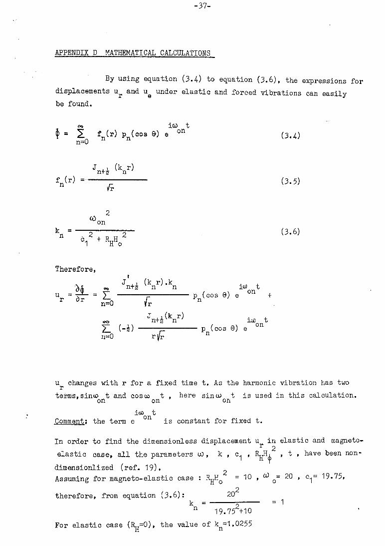
APPENDIX D MATHEMATICAL CALCULATIONS

By using equation (3»4-) "to equation (3#6), the expressions for

displacements u^ and u^ under elastic and forced vibrations can easily be found.

f 1 £nM P (cos 9) an=0

ico t on (3.4)

f (r) =n

J i (k r) n+2 n

7v(3.5)

COon

k n " *i2 ♦ V o 2

(3.6)

Therefore,

J ! (k r) .k oo n+a n n

r dru E ---- f

n=0 yr

oo

E (-4) -n=0

iuJ tp (cos 0) e on +

J ,i(k r) n+g n

fp (cos 9) e n

iiO t on

u_ changes with r for a fixed time t. As the harmonic vibration has two

terms, sinoo t and cosco t , here sinu; t is used in this calculation, on on on

iuo tComment: the term e is constant for fixed t.

In order to find the dimensionless displacement u in elastic and magneto-r 2

elastic case, all the parameters 00 , k , c , , t , have been non-

dimensionlized (ref. 19). ^Assuming for magneto-elastic case : R^Ho = 10 , ^ q= 20 , c^- 19.75,

2therefore, from equation (3.6): 20

k = ------ o----- = 1n 19.75+10 ’

For elastic case (R =0), the value of k =1.0255n n

-38-

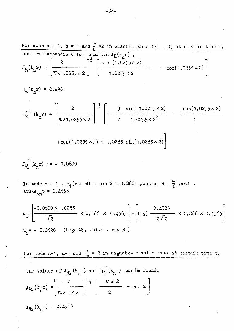
For mode n 3 1, a = 1 and — =2 in elastic case «---------- ------— ___________ a_____________________

(Rg = Q) at certain time t,

and from.appendix C for equation J^(k^r)

V knr) =.TC* 1.0255* 2

J+j(knr) = 0.4-983

sin (1.0255* 2)

1 . 0255 *2- cos(1.0255 * 2)

Jfc (knr) =

- 12

1 r2

*.*1.0255*2 L

3 sin( 1.0255* 2) cos(1 .0255X2)----------------- ---- + ------------------

2 1.0255^2 2

+cos(1.0255X2) + 1.0255 sin(1.0255x 2)

Jv (k r) .■ = - 0.0600Ti s n

In mode n = 1 , p^(cos 6) = cos 0 = 0.866 ,where 0 = -g , and

sintOon^ = 0.4-565

-0.0600x 1.0255u = r ^2

X 0,866 X 0.4.565 1 ( - 4 )0.4983

zfzK 0.866 * O .4565

u = - 0,0520 (Page 25, col.4- , row 3 ) r

For mode n=1, a=1 and3?- = 2 in magneto- elastic case at certain time t,

tne values of (k r), and «% U nr) can be foundi

(k r) =“ . 2 ‘ ,1Î3 sin

_7tX 1 * 2 . _ 2- 00s 2

J ^ ( k n r) = 0.4913

-39-'i

(knr)' 2 •

—

3sin 2 _ 4. cos 2

_ * * 2 . 2 22 2+ cos 2 + sin 2

J* ' (knr) = - 0.0315

therefore the value of u can also be found.. r

ur-0.0315----------- X 0.866 x 0.4-565. 2 .

(-4 )T0.4913--- ----X 0.866 x 0.45652 V 2

u =-0.0431 (Page 25, col. 5, row 3) r

-40-

For mode n~2 , a=1 , and -=2 , in elastic case ( R =0 ) at certain time t , * ■ -----—— ---- -------a __________________ n_______________________ _

and from appendix C for equation J^ik^r) ,

Jv (k r) =7i n2x1.0255x2

71

- 1.0255 Sin (1.0255* 2 )

2 cos ( 1.0255x2) 2 sin(1.0255X2)

Jy (k r) = - « n

Jy (k r) = 7» n

Jy (k r)= 1.17 n

22 1.0255X23

8.64.63x IQ’3

2*1.025512 1.02552 cos (1.0255x2)

TLm — _ b$ 1.0255 sin(1.0255x2) c o s (1. 0255X2)

2 21/2 22{z

.17

1.0255x 23/ 2

In mode n=2 , p^cos 0) = i (3cos20 +1)

= 0.625

sino) t = 0.685 on

The value u^ can be found by substituting all values into the equation u^.

On the graph, the numerical values are magnified twice their original values

to get a better picture of the graph.

u = r

1.17x1.0255

{2-xO. 625*0.685

r -8.6463X10“ 3(-4) 2jf2

X 0.625 x 0.685 X 2

u = 0.72763 (Page 25, col.6,row 3) r

- 4.1 -

Formode:.n=2,, a=1 , and -=2 , in magneto-elastic case at certain time t, ---- —------- — ------------ 3,________________________. .. ... — -the values of J^(k^r) and (k^r) can ^e P°un( "

r) -/*. n

—

2 * 1 X 212 - sin 2 2 cos 2 2 sin 2

-

Tl> 2 22T

2 3-

J^(knr) = -0.0217

% (V } =

2* 112.

-cos 2 1 5 sin 2 cos 2

••

5 sin 2?Z fz 2 zfz zz[z 23 l/~2

Cknr) = 1*138

In mode n=2 , p0(cos 9) = 0.625

sinco t = o.685 on

The values u^ can be found by substituting all values into the equation uf.

On the graph, the numerical values are magnified twice their original

values to get a better picture of the graph.

u = r

1.138

h< 0.625 * 0.685

u = 0.6920 (Page 25,col.7,row 3) r

(-i)-0.0217

2 ^ 2* 0.625 x 0.685 x 2

J

- 42 -

In elastic case,' for zero mode n=Q , a=1 and " = 2 at certain —— __________________________________ a--------- ,— -----time t .

Jj(knr) =

J* (knr) =

Jj(knr) =

^ ix* (k r) n

sin (k r) n... (from appendix C)

r l i. Ttx 1.0255 * 2 _

0.4941

sin ( 1.0255 X 2 )

J, (k r) = S n

2 i " k cos(k r) n n

sin(k r) n

1K k

L n _ 1

‘ r / r' 1

(knr) “f c * 1.0255,

j£-'(knr) •= -0.3876

. .(from appendix C)

1.0255 cos(1.0255 x 2) sin(1.0255 x 2)-------------------- - i -f z 2 / 2

In zero mode n=0,

pQ(cos 9-)= 1 and

sin«D t = 0.685 on

the value u can be found by substituting all the values into the equation u ,r

On the graph, the numerical values are magnified twice their originalvvalues

to get a better picture of the graph.

r

u =r

-0.3876xi.0255

hx 0.685

0.4941J ----------- X 0.685

2/2x 2

u = -0.50454 ( PaSe 25,col.2,row3) r

-4-3-

I* •In magneto-elastic case for mode n=0 , a=1 , and - =2 at certain time t,—'1 - __________ . . . ■

the values of (k r) and (k r) can be found.5 n 2 n

Ji (k r) i n '

2ft*1 X 2

j,2sin ( 1 * 2)

J;(kr) = 0.5130 5 n

Ji

(k r) = ' n

— —2

15 1 x c o s (1 a 2) sin (1 x 2)1

K x 1{2 * 21/2

(k r)= -0.3630

In mode n=0 , p (cos 0) = 1 o

sin 40 t = 0.685 on

The values u^can be found by substituting all values into the equation u^.

On the graph, the numerical values are magnified twice their original

values to get a better picture of the graph.

>4 2

u = -0.4.759 ( Page 25,col.3,row 3)r

u = r

-0.3630* 1

/2a 1 x 0.685 (-4)

0.5130

2 (2* 1 0.685

All the values of u of table A.1 in page 25 have been calculated similarly.r