A Theory of Attribution

Barry E. Feldman∗

May 29, 2007Version 1.1

abstract

Attribution of economic joint effects is achieved with a random ordermodel of their relative importance. Random order consistency and ele-mentary axioms uniquely identify linear and proportional marginal attri-bution. These are the Shapley (1953) and proportional (Feldman (1999,2002) and Ortmann (2000)) values of the dual of the implied cooper-ative game. Random order consistency does not use a reduced game.Restricted potentials facilitate identification of proportional value deriva-tives and coalition formation results. Attributions of econometric modelperformance, using data from Fair (1978), show stability across models.Proportional marginal attribution (PMA) is found to correctly identifyfactor relative importance and to have a role in model construction. Aportfolio attribution example illuminates basic issues regarding utility at-tribution and demonstrates investment applications. PMA is also shownto mitigate concerns (e.g., Thomas (1977)) regarding strategic behaviorinduced by linear cost attribution.

JEL Classifications: C10, C52, C71, D00, G11, M31 and M41.

Keywords: Attribution, coalition formation, consistency, cost allocation,joint costs, joint effects, proportional value, random order model, relativeimportance, restricted potential, Shapley value and variance decomposi-tion.

∗Prism Analytics (barry@prismanalytics.com), Russell Investment Group (bfeldman@russell.com) and DePaul University (bfeldma2@depaul.edu). Thanks for comments to Pradeep Dubey,David K. Levine, Herve Moulin and an anonymous referee. Questions and comments welcome.c©2007 by Barry Feldman.

What is the relative importance of factors influencing teenage pregnancy or globalwarming? How should corporate costs or profits be allocated? And what is therelative importance of assets in an investment portfolio?

This paper presents an economic theory of attribution capable of addressing thesequestions that is based on the general question: “What is the probability that anyorder of model factors is correctly ordered by their relative importance?” Elemen-tary axioms identify two probability distributions over factor orders. In proportionalmarginal attribution (PMA), a factor’s expected contribution share is equal the prob-ability it is most important. In linear attribution (LA) all orders are equally likely.

This work is based on and contributes to cooperative game theory, a mathematicalapproach to the study of bargaining. Cooperative game theory provides models forthe representation of the joint effects inherent in bargaining and methods for theirattribution. The simplest n-person bargaining game provides a sturdy but limitedmodel of bargaining, yet a perfect structure for the attribution problems studied here.

von Neumann (1928/1952) first defines the n-person cooperative game. The Shap-ley (1953) value is today the central solution concept. A versatile axiomatically de-fined mathematical structure, it is also the equilibrium outcome of noncooperativebargaining games such as Gull (1988) and Hart and Mas-Colell (1996). It and its gen-eralization to games with a continuum of players, the Aumann-Shapley (1974) value,have been applied to diverse problems, including cost allocation (e.g., Shubik (1962)and Young (1985)), general equilibrium (e.g., Shapley (1964)), and price setting (e.g.,Billera and Heath (1982)). Roth (1988) and Hart (2006) provide reviews.

Shapley (1953) shows his value represents the expected marginal contributions ofplayers to a growing coalition when all orders of “arrival” are equally likely. Weber(1988) characterizes the set of all linear random order values. A significant literaturehas developed (e.g., Khmelnitskya (1999) and Segal (2003)). Linearity, however,prevents the worths of coalitions from influencing the random order arrival process.

Consistency in cooperative games has been based on special games that “reduce”players from an initial game. If a solution concept is consistent, allocations to theremaining players are unchanged. Hart and Mas-Colell (1988) define a reduced gameand use it to characterize the Shapley value with consistency. Feldman (1999, 2002)shows parallel results for the proportional value using the same reduced game.

Random order consistency requires that an inert player or factor, one having nojoint effects with others, not disturb the probabilities of suborders in which it is notincluded. The random order approach to consistency does not require a reducedgame. This facilitates practical application. Random order consistency is shown toprovide a simple and powerful expectations-based approach to cooperative value.

The proportional value (Ortmann (2000) and Feldman (1999, 2002)) satisfies aproportional gain rule instead of the balanced (equal) contributions rule of Myerson(1980) and is defined by a ratio potential rather than the linear Hart and Mas-Colell(1988) potential. Feldman (2002) shows the proportional value induces a random

order process influenced by coalitional worths and that it is the equilibrium outcomeof a noncooperative bargaining game where players’ probabilities of proposing areproportional to their expected payoff. Khmelnitskya and Driessen (2001) and Calvoand Driessen (2003) study generalizations.

Section 1 of this paper presents a microeconomic model of relative importancebased on set marginal contributions in a random order model. Random order consis-tency and other axioms are used to directly identify a probability distribution overorders. The Shapley and proportional values are identified in a common framework,without assuming linearity or proportionality, though the change of a single axiom.

Section 2 defines restricted potentials and obtains proportional value derivativesand coalition formation results. The proportional value is shown not converse mono-tonic. A family of values including the Shapley and proportional values is shown.

* * *

Attribution involves a single monotonic utility function. Players in the correspondingbargaining problem must be assumed to have identical linear utility functions. Inattribution, factors and factor sets replace players and coalitions. The worth of afactor set is based on the utility resulting from the presence of its factors or therestriction of utility maximization to the variation of its factors. Three examplesdemonstrate the potential of this theory of attribution.

Statistical tests ignore joint effects by design. Linear attribution of OLS R2 asa measure of relative importance is proposed by Hoffman (1960), Lindeman, et al.(1980), Kruskal (1987) and Chevan and Sutherland (1991). McNally (2000) initiatesits use in ecology studies. Soofi, et al. (2000) develop a model of linear attribution incategorical analysis. Linear attribution of model R2 allows a factor to appear impor-tant due only to correlations with factors in the true model. Feldman (2005a) firstproposes an exclusion axiom which requires that such a factor receive zero attribu-tion share, and with other axioms, characterizes proportional marginal attributionof model R2 (there called proportional marginal variance decomposition or PMVD).Gromping (2006, 2007) provides attribution tools and studies OLS LA and PMA.

Section 3 studies econometric attribution. The model objective function is con-sidered to be the utility function of an analyst. Random order consistency is foundcompatible with econometric attribution. Attributions are found stable and compa-rable across a variety models based on data from Fair (1977). PMA identifies factorrelative importance and model relationships missed by joint significance tests.

Section 4 considers utility attribution in microeconomic models more generally.Random order consistency is found to be an acceptable axiom whenever an attributionproblem can be composed with an independent problem. A portfolio optimizationexample illustrates utility attribution in a typical microeconomic context. The exam-ple provides methods for evaluating the relative importance of assets in an investor’sportfolio and the per-dollar contributions of assets to investor utility.

2

Section 5 considers cost allocation as an attribution problem. Random orderconsistency is found to be an appropriate axiom for cost attribution. An exampleillustrates the relative vulnerability of LA to strategic definition of cost centers.

The conclusion summarizes, compares random order and reduced game consis-tency and considers the common assumption that proportional solutions are transla-tion dependent in the light of results of developed here. Extended proofs follow.

1 Basic results

1.1 General framework

Transferrable utility (TU) games represent the worth of a coalition by a single number.Let N = 1, 2, . . . , n be the players or factors. A standard TU game v is a mapv : 2N → R+ ∪ 0 from all S ⊆ N to the nonnegative real numbers, with v(∅) ≡ 0.The S ⊆ N are coalitions or factor sets. Let i = i and 12 = 1, 2. Set subtractionof i from S is written S \ i. Games are assumed weakly monotonic: v(S ∪ i) ≥ v(S).

In an attribution problem, v(S) is the expected utility of a single decision maker.If S represents binary characteristics, then v(S) is the utility resulting from the jointpresence of the factors.1 Factor set S may instead provide the decision maker withdecision space ∆S, with σS ∈ ∆S being a possible choice. Then v(S) is the maximum

v(S) = maxσS∈∆S

U(σS)− U(∅), (1)

where the null utility U(∅) represents the utility obtained when there are no opti-mization choices. The null utility is the basis point of Feldman (2005b). It is clearlyneeded with exponential and other utility functions that can generate negative utility.Its importance in other circumstances will become apparent.

The weak monotonicity of v corresponds to the assumption that maximizationover a greater number of factors cannot result in a decline in expected utility.

The dual game to v represents the marginal contributions of all coalitions or factorsets. The dual worth w(S) is v(N) minus the worth of the complement of S:

w(S) = v(N)− v(N \ S). (2)

1.2 The random order model

Attribution is based on a random order model of relative importance. A discretemarginality replaces the more typical economic focus on continuous marginal condi-tions. In this model factors “arrive,” one at time, to join a growing factor set. Factors

1A monotonic cover game, where v∗(S) = maxR⊂Sv(R), can be used to ensure monotonicity.

3

could be indexed by arrival order. However, due to the central role of joint marginalcontributions, it is simpler to consider the “last to arrive” as the first in an order.The last to arrive can instead be thought of as “first to leave.”

An order r = (r1, r2, . . . , rn) is a permutation of the factors (or players) of N . Theset of all orders of N is R(N). Define Sr

k = r1, . . . , rk to be the set (coalition) ofthe first k factors (players) in the order r. These are the last k factors to arrive inorder r. If S has k factors, S is included in r, written S ∈ r, if and only if S = Sr

k.Thus w(Sr

i ) is the joint marginal contribution of the last i factors to enter. Let r(i)be the position of i in order r, so that rr(i) = i. When factors are ordered accordingto relative importance, r1 is least important and rn is most important.

Let rS be an order of the factors of a set S ( N and consider an r ∈ R(N). Assumethat for any i and j in S such that rS(i) > rS(j), it is also true that r(i) > r(j). Theorder of the factors in rS is preserved in r, so rS is a suborder of r, written rS ⊂ r.Also, r is a superorder of rS, written r ⊃ rS.

Let mP (r) be an n-vector of positional marginal contributions defined by r. Ele-ment i, mP

i (r), represents the marginal contribution of the factor in position i in r.This quantity is defined as follows with respect to the dual game:

mPi (r) = w(Sr

i )− w(Sri−1), i = 1, 2, . . . , n, (3)

where Sr0 = ∅ and w(∅) = 0. Let mS(r) be the n-vector of set marginal contributions:

mSi (r) = w(Sr

i ) = v(N)− v(N \ Sri (r)), i = 1, 2, . . . , n. (4)

The probability p(r) that any order r ∈ R(N) is the realized order of arrivals isdefined by a likelihood function L(r) with L(r) ≥ 0 for all r:

p(r∗) =L(r∗)∑

r∈R(N)

L(r). (5)

The expected utility contribution of factor i with respect to distribution p is then

φi(v) = Ep[mPr(i)(r)] =

∑

r∈R(N)

p (r) mPr(i)(r). (6)

1.3 Axioms and the fundamental theorem

Axioms are used to identify probability distributions over orderings and not the valuefunction itself. Such a distribution may be understood to represent the probabilitythat any order is correctly ordered by the relative importance of its factors.

4

A factor z is inert if and only if it adds exactly its own non-zero worth to everycoalition: v(z) > 0 and, for any S ⊆ N \ z, v(S ∪ z) = v(S) + v(z). Let v∗ be thegame created by adding a set of inert factors Z, so that N∗ = N ∪ Z.

Axiom 1.1 Random order consistency: p (r | v) =∑

r∗∈R(N∗)r∗⊃ r

p (r∗| v∗).

Random order consistency requires that an inert factor or factor set have no effecton the probability of any suborder of the remaining factors. Consider an order r inR(N). Then the sum of the probabilities of all orders r∗ ∈ R(N∗) such that r ⊂ r∗

relative to the game v∗ must equal the probability of r relative to v.

If the axiom holds for a likelihood L in games of cardinalities m and n, then L israndom order consistent between these cardinalities. If L is random order consistent,then it is random order consistent between all cardinalities m and n, 2 ≤ m < n.

Compared to Hart and Mas-Colell (1988) reduced game consistency, random orderconsistency requires the existence of inert factors, but does not require a reduced gameor directly constrain value allocation when inert factors are not present.

Axiom 1.2 Exclusion: If mS1 (r) = 0 when r(z) = 1 and mS

1 (r∗) > 0 when r∗(j) =1, for all j 6= z, then for any r∗ such that r∗(z) > 1, p (r∗) = 0.

Assume z makes zero final marginal contribution (arriving last in any order r) andall other factors make positive final marginal contributions. Exclusion then requiresthat only orders where z arrives last are assigned positive probability.

The basic idea of exclusion is that a factor making zero final marginal contributionshould receive no attribution share. This outcome, however, is not demanded whenthere are two or more such factors (cf., Feldman (2002), Section 6.1).

Exclusion will considered in the limit as marginal contributions grow small. Let v0

be strictly monotonic. Define a sequence of games v1, v2, . . . , v∞ where vt(S) = v0(S)for S 6= N \ z and limt→∞ vt(N \ z) = v0(N). If r(z) = 1 then limt→∞ mS

1 (r| vt) = 0.Exclusion requires that if r∗(z) > 1, then limt→∞ p (r∗| vt) = 0.

Axiom 1.3 Separability: L(r) =∑

li(mSi (r)) or L(r) =

∏li(m

Si (r)).

Separability requires the likelihood function be a sum or product of subliklihoods.Separability limits complexity but does not imply separability of p or φ.

Axiom 1.4 Anonymity: If mS(r∗) = mS(r), then L(r∗) = L(r).

Anonymity requires L(r) depend only on the marginal contributions of the factor setsincluded in r.

5

Axiom 1.5 Inclusion: If mSr(i)(r) > 0, then there is an r∗ such that p (r∗) > 0 and

mPr∗(i)(r

∗) > 0.

Inclusion requires that if a factor makes a positive positional contribution in any orderr that there must be an order r∗ with positive probability in which the factor alsomakes a positive positional contribution. It could be that r∗ = r.

The following result is proved in the next two subsections.

Theorem 1.1 (The Fundamental Theorem of Attribution) Let v be a gamerepresenting an attribution or bargaining problem, and let w be its dual. Requirethat the value attributed to factors or players equal the their expected marginal contri-bution resulting from a probability distribution over orders in the random order modelof relative importance.

(i) The Shapley and proportional values of w, corresponding to linear and propor-tional marginal attribution, are the only random order consistent, anonymousand separable values.

(ii) The Shapley value of v is the unique value that additionally satisfies inclusion.

(iii) The proportional value of w uniquely additionally satisfies exclusion.

Remark 1.1 Random order consistency is uniquely associated with cooperative value.The reduced game approach only establishes consistency with respect to a particulartwo-player solution. Complete characterization requires specific axioms for the two-player case (e.g., Hart and Mas-Colell (1988), Theorem B’). Many solution conceptsare consistent with respect to the Hart and Mas-Colell reduced game, including equalsplit, average cost pricing, serial cost sharing (Moulin and Shenker, 1992), fixed pro-portions, path methods (Friedman, 2004), dictatorial and priority rules (see Leroux(2006) for further discussion). An additional complication of the reduced game ap-proach is still other solutions are consistent with respect to other reduced games.

1.4 Relative importance likelihood functions

A likelihood L is exogenous if it is independent of v, i.e., ∂L(r)/∂v(S) = 0 forall r ∈ R(N) and S ⊆ N . If L is not exogenous, it is endogenous. Random orderconsistency, anonymity and inclusion identify a unique exogenous likelihood. Randomorder consistency, separability and exclusion identify a unique endogenous likelihood.

Lemma 1.1 The unique (up to scaling) endogenous separable likelihood function thatsatisfies random order consistency is

L¦(r) =

( ∏S∈ r

w(S)

)−1

.

6

Further, L¦ is anonymous and positive.

Proof: See Appendix A (Sec. 7.1).

Lemma 1.2 The likelihood function L∗(r) = c > 0 with p(r)=1/n! is uniquely iden-tified (up to scaling) by anonymity, inclusion and random order consistency. It alsoformally satisfies both additively and multiplicative separability.

Proof: L∗(r) is anonymous and p(r) = 1/n! for any L∗ = c > 0. It is inclusive since forall r, p(r) > 0. It is random order consistent since for any r0 in N \ z, where z is inert,∑

r⊃r0p(r) = n/n! = 1/(n − 1)!. Inclusion is necessary since L¦ satisfies anonymity

and random order consistency. Random order consistency is necessary because manylikelihoods satisfy anonymity and inclusion, e.g., Lo(r) =

∑S∈r w(Sr

i ). It is sufficient

to show the necessity of anonymity when n ≤ 3: Let lωi (Sri ) = ωr(i)/

∑ij=1 ωr(j) and

Lω(r) =∏

lωi (Sri ), where ωi > 0, i = 1, 2, 3, are exogenous weights. Lω is inclusive.

It is easy to determine that Lω((1, 2, 3)) + Lω((1, 3, 2)) + Lω((3, 1, 2)) = Lω((1, 2)).(This is the weight system of the weighted Shapley value, cf., e.g., Kalai and Samet(1987).) Thus, Lω is random order consistent for m = 2 and n = 3 and anonymityis necessary. Let l∗i (S) = c1/n, L∗(r) =

∏ni=1 l∗i (S) = c and L∗ is multiplicatively

separable. Let l∗i = c/n, L∗(r) =∑n

i=1 l∗i (S) = c and L∗ is additively separable. ¤

Lemma 1.3 L¦ is the unique likelihood function to satisfy separability, random orderconsistency and exclusion.

Proof: L∗ cannot satisfy exclusion as p(r) > 0 for all r ∈ R(N). L¦ satisfies exclusion.To see, consider an dual attribution problem w0 where the final marginal contributionof z is very small and a sequence of games wt∞t=1, where limt→∞ wt(z) = 0; butfor all other sets S ⊆ N , wt(S) = w0(S) > 0. For any rΩ ∈ R(N) such thatrΩ1 = z, limt→∞ L¦t (r

Ω) = +∞, however, clearly p¦t (rΩ) = L¦t (r

Ω)/∑

r∈R(N) L¦t (r) ≤ 1.

Further, for any r∗ with r∗1 6= z, limi→∞ p¦t (r∗) = L¦t (r

∗)/∑

r∈R(N) L¦t (r) = 0 since

limt→∞ L¦(r∗)/L¦(rΩ) = 0. A non-anonymous exogenous L could assign an r ∈ R(N)zero probability, but exclusion would not be satisfied. ¤

Remark 1.2 Note that all separable likelihood functions with li(•) = lj(•) are randomorder consistent when likelihoods are based on positional marginal contribution.

1.5 Attribution and value

The Shapley values of v and its dual w are equal and are the expectation when L∗ isused in (6). Thus Lemma 1.2 proves

7

Theorem 1.2 Let the likelihood of the distribution over orders in the random or-der model of relative importance satisfy random order consistency, anonymity andinclusion. Then the resulting attribution is equal to the Shapley value of the problem.

Remark 1.3 Weighted Shapley (1953) values might be identified by random orderconsistency and inclusion (as suggested in the proof of Lemma 1.2).

Define the function P (S) for any S ⊆ N as

P (S) =

∑

r∈R(S)

L¦(r)

−1

. (7)

P (N) is then the normalizing factor that relates L¦ to the implied distribution p¦:

p¦(r) = P (N)L¦(r). (8)

Feldman (2002), Lemma 2.1 shows that formula (7) is one form of the ratio potentialof a cooperative game and that P (S) is also recursively defined by the formula

P (S) = w(S)

(∑i∈S

P (S \ i)−1

)−1

. (9)

Substitution of formula (8) into the expectation (6) gives

ϕi(w) = P (N)∑

r∈R(N)

L¦(r)mPr(i)(r). (10)

Lemma 1.4 P (N \ i) =

∑

r∈R(N)

L¦(r) mPr(i)(r)

−1

.

This is proved in Appendix B (Sec. 7.2) and by Feldman (2002), Lemma 2.9.

Corollary 1.1 ϕi(w) =P (N)

P (N \ i).

The discrete derivative of the ratio potential with respect to i is one definition of i’sproportional value (Feldman (1999) equation (3.6), Ortmann (2000) Definition 2.2).Thus Lemma 1.1, expectation (10) and Lemma 1.4 prove

Theorem 1.3 Let the likelihood of the distribution over orders in the random ordermodel of relative importance satisfy random order consistency, exclusion and separa-bility. Then the attribution of v is equal to the proportional value of w, its dual.

8

2 Properties of the proportional value

2.1 Elementary properties

Random order consistency directly implies the following lemma, where ϕ(v, S) is theproportional value of v when v is limited to the factors in S.

Lemma 2.1 If z is inert then ϕi(v, S \ z) = ϕi(v, S).

Now let N = 1, 2. Then P (i) = w(Siji ) = w(i) = v(12)− v(j) and

P (12 ) =w(12 )

P (1)−1 + P (2)−1=

w(12)

w(1)−1 + w(2)−1=

w(1)w(2)w(12)

w(1) + w(2),

so that

ϕi(w) =P (N)

P (N \ i)=

w(i)

w(1) + w(2)w(12). (11)

Myerson (1980) shows the Shapley value is defined by balanced contributions:

Shi(S, v)− Shi(S \ j, v) = Shj(S, v)− Shj(S \ i, v).

Adding j to S helps i in the same measure that adding i helps j. Ortmann (2000),Theorem 2.6 characterizes the proportional value with an analogous ratio perservingcondition (called equal proportional gain in Feldman (1999 and 2002)):

ϕi(S, v)

ϕi(S \ j, v)=

ϕj(S, v)

ϕj(S \ i, v). (12)

Lemma 2.2 Let v be a cooperative game with n players and require c > 0.

(i) Let v∗(S) = v(S) if |S| 6= k for a k < n and v∗(S) = v(S) + c when |S| = k.

Then Sh(v∗) = Sh(v).

(ii) Let v∗(S) = v(S) if |S| 6= k for a k < n and v∗(S) = c v(S) when |S| = k.

Then ϕ(v∗) = ϕ(v).

(iii) Let v∗(S) = v(S) if S 6= N and v∗(N) = v(N) + n c.

Then Sh(v∗) = Sh(v) + c.

(iv) Let v∗(S) = v(S) if S 6= N and v∗(N) = c v(N), v∗ still monotonic.

Then ϕ(v∗) = c ϕ(v).

9

Proof: The Shapley results are obvious. Proportional value results follow directlyfrom formulas (7) or (9) and Corollary 1.1. ¤

Corollary 2.1 The proportional value is the unique random order consistent andseparable value in the random order model of relative importance that (a) is invariantto a proportional change in the worth of all coalitions of any cardinality s < n or (b)scales with changes in v(N).

2.2 The probability of being most important

Lemma 2.3 The probability that factor i is most important in a proportional marginalattribution is ϕi(w)/w(N).

Proof: The probability of i being most important in a PMA implies arriving first inthe random order model of relative importance. This also implies being in positionn and that worths are relative to the dual game w. Thus

p (rn = i|w) = P (N,w)∑

r∈R(N)r:rn=i

n∏i=1

w(Sri )−1

=P (N, w)

w(N)P (N \ i, w)=

ϕi(w)

w(N).

The first line above follows from formula (8), The substitution on the second linefollows from factoring out w(N) and applying Lemma (1.4). ¤

2.3 Your enemy’s enemy may be your friend

Feldman (1999), Lemma 3.5, shows the proportional value is monotonic. It is shownhere the proportional value is not converse monotonic. The value of i can increasewith an increase in the worth of S even if i 6∈ S.

The restriction of a game v by a coalition S∗ includes only coalitions T ) S∗ thatinclude S∗ as a proper subset. Let RP (S∗, S) be the restricted potential for S in vrestricted by S∗. Define RP (S∗, S∗) = 1 and define RP as in the following lemma.

Lemma 2.4 For any T : S∗ ( T ⊆ N ,

RP (S∗, T ) = v(T )

∑

i∈T\S∗RP (S∗, T \ i)−1

−1

=

∑r∈R(T )S∗=Sr

s

∏S∈r

S)S∗

v(S)−1

−1

.

10

The first part of the equivalence is the definition. The proof of the second equivalenceis by recursive substitution, as in Feldman (2002), Lemma 2.1. The value of a playeri 6∈ S∗ in the game v restricted by S∗ is ϕi(S

∗, N, v) = RP (S∗, N)/RP (S∗, N \ i).

Lemma 2.5 The derivative of ϕi(v) with the worth of any coalition S∗ ⊂ N is

∂ϕi(v)

∂v(S∗)=

ϕi(v)P (N)

v(S∗)P (S∗)RP (S∗, N), i ∈ S∗,

ϕi(v)1

v(S∗)P (S∗)

(P (N)

RP (S∗, N)− P (N \ i)

RP (S∗, N \ i)

), i 6∈ S∗.

Proof: The result follows from the value of ∂P (S)/∂v(S∗) for any S : S∗ ( S ⊆ N .

∂P (S)

∂v(S∗)= [P (S)]2v(S∗)−1

∑

r3v(S∗)

∏S∈r

v(S)−1

= [P (S)]2[v(S∗)P (S∗)RP (S∗, N)

]−1

The first result is from straightforward differentiation. The second result follows asthe sum of products in the first is equal to [P (S∗)RP (S∗, S)]−1 for S ) S∗. ¤

It follows that ∂ϕi(v)/∂v(N) = ϕi(v)/v(N) (thus∑

i∈N ∂ϕi(v)/∂v(N) = 1) andthat ∂ϕi(v)/∂v(S∗) > 0 for an i ∈ S∗. On the other hand, the sign of ∂ϕi(v)/∂v(S∗)is not clear for an i 6∈ S∗. Multiplying the LHS and RHS results of Lemma 2.5 byRP (S∗, N)/P (N \ i) shows

∑i∈N ∂ϕi(v)/∂v(S∗) = 0 and the following.

Corollary 2.2 For any i ∈ N \ S∗,∂ϕi(v)

∂v(S∗)∝ ϕi(v)− ϕi(S

∗, N, v).

If i’s value in v restricted by S∗ is less than in v, then ϕ is not converse monotonic.This seems possible since formula (11) shows that adding a c > 0 to all worths canreduce the value of a dominant player. The Shapley and weighted Shapley values areconverse monotonic of their linearity.

Table 1 presents an example that demonstrates the proportional value is not con-verse monotonic. In v, 1 is weakest and 3 is strongest. 2 is strong in combinationwith 3, but less so in combination with 1. The proportional value (ϕ), the Shapleyvalue (Sh) and the nucleolus (Nuc) all provide qualitatively similar allocations.

The game v∗ is a version of v modified only by increasing 1’s individual worth to10. The proportional value is not converse monotonic because 3’s value is larger thanin v. Further, player 1’s share of value and dominance over the next largest playerhave both increased. This appears a plausible outcome in economic, political andmilitary competition. The Shapley value shows similar allocations before and after,with 2 still stronger than 1. The nucleolus (Schmeidler, 1969) does not change.

11

v(1) = 1, v(2) = 2, v(3) = 25,v(12 ) = 20, v(13 ) = 30, v(23 ) = 60,

v(123 ) = 100

v∗(S) = v(S), S 6= 1, v∗(1) = 10

ϕ1(v) = 7.58, ϕ2(v) = 29.21, ϕ3(v) = 63.20ϕ1(v

∗) = 20.61, ϕ2(v∗) = 10.69, ϕ3(v

∗) = 68.70∆ϕ1 = 13.03, ∆ϕ2 = −18.52, ∆ϕ3 = 5.50

Sh1(v) = 17.50, Sh2(v) = 33.00, Sh3(v) = 49.50Sh1(v

∗) = 20.50, Sh2(v∗) = 31.50, Sh3(v

∗) = 48.00∆Sh1 = 3.00, ∆Sh2 = − 1.50, ∆Sh3 = − 1.50

Nuc1(v) = 12.00, Nuc2(v) = 36.00, Nuc3(v) = 52.00Nuc1(v

∗) = 12.00, Nuc2(v∗) = 36.00, Nuc3(v

∗) = 52.00∆Nuc1 = 0.00, ∆Nuc2 = 0.00, ∆Nuc3 = 0.00

Table 1: Your enemy’s enemy may be your friend.

Corollary 2.3 The Shapley value is the unique random order consistent, anonymous,separable and converse monotonic value.

2.4 Coalition formation

Simple coalition formation results are implied by Sections 2.2 and 2.3. The coalitionS forms if its members all arrive before any members of N \S. Lemma 2.3 implies theprobability that i is most important and j is second most important in the randomorder model of relative importance is ϕi(N, w)/w(N)× ϕj(N \ i, w)/w(N \ i), or, interms of potentials, P (N, w)/P (N \ ij, w) × [w(N)w(N \ i)]−1. When the probabil-ity that S forms is summed over all such orders, the sum of worth products is therestricted potential RP (S,N, w). Results change in a standard random order modelbased on v, where the first in an order is the first to arrive. The player arriving lastis now most important. If one player has zero individual worth, this player will arrivefirst with probability one (and receive zero value, see Feldman (2002), Section 6).Then the probability of S forming in v is the probability that N \ S arrive last.

Lemma 2.6 The probability of a coalition S forming in the random order model ofrelative importance is

p(S|w) =P (N,w)

P (N \ S,w) RP (N \ S, N, w),

12

where P (∅, w) ≡ 1 and RP (∅, N, w) ≡ P (N, w). The probability that S forms in arandom order model of the proportional value based on v instead of its dual is

p(S| v) =P (N, v)

P (S, v) RP (S,N, v).

Corollary 2.4 The derivatives of the proportional value for any member i ∈ N rel-ative any S ⊆ N in the game v or its dual w are as follows.

∂ϕi(v)

∂v(S)=

ϕi(v)

v(S)p(S| v), i ∈ S,

ϕi(v)

v(S)

[p(S, N | v)− p(S,N \ i | v)

], i 6∈ S, and

∂ϕi(w)

∂w(S)=

ϕi(w)

w(S)p(N \ S|w), i ∈ S,

ϕi(w)

w(S)

[p(N \ (S ∪ i), N |w)− p(N \ (S ∪ i), N \ i |w)

], i 6∈ S.

This corollary results from substitution of the results of Lemma 2.6 into Lemma 2.5.(Note that for any i ∈ S, ∂Shi(v)/∂v(S) = 1/s pSh(S| v) = (s − 1)!(n − s)!/(s n!).)This corollary provides the intuition that the proportional value is not converse mono-tonic for an i with respect to S 63 i in v when the importance of S (the probabilityof forming) is greater in N than in N \ i. The probability that S arrives and then iis determined by Lemma 2.6, giving the following (computationally very inefficient)representation of the proportional value in classical marginal contribution form.

Corollary 2.5

ϕi(v) =∑

S⊂N \i

P (S ∪ i)P (N)

v(i)RP (i, S ∪ i)P (S) RP (S, N)

(v(S ∪ i)− v(S)

).

2.5 Linear-proportional family of values

Feldman (2005) Section 5.1 shows the linear and proportional values are both includedin a one-parameter family of values. This family results from replacing random orderconsistency with a weaker axiom, which requires that effect on likelihood of a marginalchange of the worth of any coalition Sr

i included in an order r be the same.

Axiom 2.1 Proportional effect:∂ ln L(r)∂ ln w(Sr

i )= α, i = 1, . . . , n.

13

It is straightforward to show that proportional effect, exclusion and anonymityidentify the following likelihood (see Feldman (2005) Sections 3.3 and 5.1)

Lα(r) =

( ∏S∈ r

w(S)

)−α

, α > 0. (13)

The case α = 0 is covered by Lemma 1.2. Define the normalizing factor Pα(N) =(∑r∈R(N) Lα(r)

)−1

, and a family of probability distributions pα, indexed by α results:

pα(r) = Pα(N)Lα(r). (14)

The induced expectation when (14) used to generate expectation (6) is is clearlythe Shapley value when α = 0 and the proportional value when α = 1. Note,however, that these are the only random order consistent members of this family andthat Pα(N) is not a potential for α 6= 1.

3 Econometric attribution

An independent variable completely orthogonal to all others in an econometric modelwill not affect their model parameters or statistical significance levels. It is inert inthe implied attribution problem. Random order consistency requires only that such avariable not affect other attributions. The theory of attribution can thus be appliedto tasks such as variance and likelihood decomposition across a wide range of models.

Proposition 3.1 If adding a factor z to an attribution problem based on likelihoodfunction increases the likelihood of the model but leaves the individual and joint sta-tistical significance of all other variables unchanged, then z is an inert factor.

Proof: Let v and v∗ represent the joint log likelihoods of factors in models based onN and N∗ = N ∪ z, respectively, with duals w and w∗. Measure the joint significanceof any factor set with the likelihood ratio test, which is based on their joint marginallikelihood contribution. Thus w∗(S) = w(S) for all S ⊆ N \ z, and v∗(N ∪ z)−v∗(N ∪z \ S) = v∗(N)− v∗(N \ S) for all S ⊆ N . Since w∗(z) > 0, z is inert in w. ¤

Exclusion requires that a factor making zero final marginal contribution to modelperformance, when all others have positive final marginal contribution, receive zeroattribution share. Such a factor will have zero statistical significance (e.g., p = 1 thatβ = 0). Exclusion makes attribution as closely related to statistical significance aspossible given the mutual correlation of explanatory factors.

Feldman (2005a) proposes four admissibility criteria for estimators of statisticalrelative importance: nonnegativity, proper exclusion (here, simply exclusion), proper

14

inclusion and full contribution. Proper inclusion requires factors making positive (fi-nal) marginal contribution receive positive attribution. Full contribution requires thatthe sum of attributions for factors in a set S equal their joint marginal contributionif they are uncorrelated with all factors in N \ S. PMA is an admissible estimator.

Feldman (2005a) also shows PMA components can be estimated consistently, de-velops properties and presents examples of LA, PMA and CVD (see fn. 4, below).Feldman (2005a) and Gromping (2007) note the potentially lower level of precisionof PMVD components.2

In econometric attribution the utility function (1) can be understood to belong toan analyst and to be the model objective or likelihood function. Since OLS maximizesR2 and R2 is set monotonic, the marginal contribution to variance or R2 can be thebasis of attribution. Measures such as adjusted R2, SIC and BIC cannot be used inattribution because they are not set monotonic. A further logical restriction for eligi-ble measures is that it should be possible to use the measure to construct statisticalsignificance tests. Such measures are more likely to be useful for the assessment ofrelative importance of model factors. F -tests can be constructed from R2 values.

3.1 Indirect effects

Gromping (2007) proposes that LA should be used when interested in indirect effects.For example, if x = f(y) and y = g(z) then z will receive a zero PMA share in theattribution of x = f ′(y, z), but will receive an LA share if x and z are directlycorrelated. The following is a direct implication of the Fundamental Theorem.

Corollary 3.1 Linear attribution is the only anonymous random order consistentattribution that recognizes indirect contributions to econometric model performance.

Indirect effects can also be explicitly attributed with an assumed non-simultaneouscausal structure. The result is a nesting of attribution problems. Owen (1977) showsthat nested games can be interpreted as a composition of random order models.

Proposition 3.2 Consider nested OLS models x = f(y) and y = g(z). The varianceof x indirectly explained by z is σ2

xR2xyR

2yz.

Proof: First, x = a+σxy/σ2yy. The projection of x on z gives x, the part of x explained

by y that is explained by z: x = b + σxz/σ2zz, where σxz = σxy/σ

2yσyz. The variance

of x is [σxyσyz]2/[σ2

yσ2z ]

2σ2z . The variance share of x thus explained by z is then

R2xz =

[σxyσyz]2

σ2x[σ

2y]

2σ2z

=ρ2

xyσ2xσ

2yρ

2yzσ

2yσ

2z

σ2x[σ

2y]

2σ2z

= ρ2xyρ

2yz = R2

xyR2yz ¤

2Gromping (2006) describes the relaimpo package for R statistical freeware, which estimatesseveral relative importance metrics for models and computes bootstrap confidence intervals.

15

3.2 The structure of econometric attributions

Econometric attribution is based on the model objective function to be maximized:

v(S) = Θ(S)−Θ(∅), for all S : S ⊆ N,S 6= ∅, (15)

where Θ(S) is the objective function value when the factors in S are in the model andthose in N \ S are not. Θ(∅) is the null utility of formula (1), the model objectivevalue when not including any factors in N . For OLS with R2 as the objective andan intercept, and when the intercept is not a factor, Θ(∅) = 0. With log-likelihoods,typically v(S) < 0 without normalization. If v∗(S) = abs[Θ(S)], v∗ is not monotonicand results are useless. Also, likelihood (e.g., v∗(S) = exp[Θ(S)]) is not a substitutefor log-likelihood because it is not used in significance tests.

Attribution shares, and not magnitudes or differences, are the essential informa-tion. It may be difficult to properly determine the null likelihood for some models.3

In such cases, linear attribution shares cannot usefully be defined because they are afunction of Θ(∅). PMA shares, however, are invariant to changes in Θ(∅), so long asmonotonicity is maintained, because in the dual game to v the worths of all S ( Nare invariant to changes in Θ(∅). Changes in the dual worth w(N) only scale PMAcomponents. These relationships are consequences of Lemma 2.2.

Corollary 3.2 Let v∗(S) = c v(S) + d, c > 0 for all S and let w∗ be the dual of v∗.Then ϕi(w

∗)/w∗(N) = ϕi(w)/w(N). PMA is share scale and translation invariant.

OLS R2 attributions sum to the R2 of the model, but can be normalized to sumto 100%. R2-like measures that indicate the relative explanatory power of some max-imum likelihood models have been constructed (see Maddala (1983), Section 2.11).

3.3 Fair’s (1978) infidelity study

Econometric attribution is studied here in the context of Fair’s (1978) study of 601responses of first-time married individuals to a 1969 sex survey conducted by Psychol-ogy Today. Fair studies the predictors of the frequency of marital infidelity. Green(2003) reanalyzes this publicly available data. Fair’s original model is first analyzedusing OLS, tobit and Poisson regression. The determinants of marital happiness arethen examined with OLS and ordered probit. In addition to model results, LAs,PMAs and covariance decompositions (CV Ds) are reported.4

3A linear model without an intercept is a simple example.4CVD is a standard approach to variance decomposition in economics and finance. The CVD

component of a factor i is βi1′NΣβ, where β is the model coefficient vector, Σ is the factor covariancematrix and 1N is a n × 1 vector of ones. See Feldman (2005a) Sections 4.3, 4.4 and 5 for resultsconcerning CVD and examples. CVD can be described as a form of LA that results when theoptimization of formula (1) is applied to only to the complete model.

16

Factor beta st. dev. t-stat. PMA LA CVD

OLSAge -0.050 0.022 -2.278 4.83% 5.73% -10.27%Years married 0.162 0.037 4.387 20.16% 23.59% 38.87%Religious -0.476 0.111 -4.279 18.92% 19.63% 18.54%Occupation 0.106 0.071 1.491 2.14% 1.84% 2.21%Happiness -0.712 0.118 -6.021 53.94% 49.21% 50.66%R2: 0.1314

TobitAge -0.179 0.079 -2.27 5.30% 5.33% -10.09%Years married 0.554 0.135 4.12 19.22% 22.64% 39.27%Religious -1.686 0.404 -4.18 20.16% 20.78% 21.30%Occupation 0.326 0.254 1.28 1.89% 1.59% 1.84%Happiness -2.285 0.408 -5.60 53.44% 49.65% 47.69%Log(scale) 2.110 0.067 31.44Model ln L: -705.5762, null model ln L: -744.7375

PoissonAge -0.032 0.006 -5.51 4.86% 5.68% -11.28%Years married 0.116 0.010 11.68 23.12% 25.71% 45.09%Religious -0.354 0.031 -11.46 20.88% 21.19% 22.95%Occupation 0.080 0.019 4.11 2.61% 2.13% 3.08%Happiness -0.409 0.027 -14.95 48.54% 45.29% 40.16%Model ln L: -1180.05, null model ln L: -1462.75

Table 2: Reanalysis of Fair (1978). Independent variable: frequency of infidelity.

The response variable studied by Fair is the self-reported frequency of infidelity.The explanatory factors include the respondent’s sex, age, education and occupation,the number of years married, whether the respondent has children and the respon-dent’s (self reported) level of religious belief and marital happiness.5

Fair excludes sex, education and having children as predictive factors based ontheir joint statistical insignificance. In attributions based on the complete model,all attribution methods assign these factors small attribution components, consistentwith their low individual test statistics. The respective t-statistics are (0.18, 0.41,0.21). The corresponding PMA components are (0.03%, 0.21% 0.05%). PMA andt-statistics can together better motivate efficient multivariate hypothesis testing thant-statistics alone. LA results, (0.15%, 3.12%, 0.29%), are not as clear for education.

5Fair (1978) provides descriptive statistics. The data set is available online.

17

Factor beta st. dev. t-stat. PMA LA CVD

OLSSex -0.070 0.103 -0.69 1.45% 0.75% 0.27%Age -0.006 0.008 -0.78 4.33% 19.92% 11.25%Years married -0.035 0.014 -2.52 58.54% 35.13% 48.50%Children -0.207 0.120 -1.74 10.74% 19.83% 18.63%Religious 0.085 0.038 2.22 7.17% 5.44% 2.43%Education 0.074 0.022 3.41 16.08% 17.71% 19.73%Occupation -0.025 0.030 -0.83 1.69% 1.21% -0.81%R2 : 0.0894

Ordered probitSex -0.092 0.106 -0.86 2.09% 1.04% 0.92%Age -0.005 0.008 -0.68 3.21% 19.72% 9.70%Years married -0.037 0.014 -2.60 58.64% 36.18% 49.57%Children -0.262 0.125 -2.09 15.60% 23.18% 23.82%Religious 0.087 0.039 2.20 6.87% 5.16% 2.07%Education 0.069 0.022 3.10 12.08% 13.70% 14.31%Occupation -0.025 0.031 -0.81 1.51% 1.03% -0.40%Model ln L: -1180.05, null model ln L: -1462.75

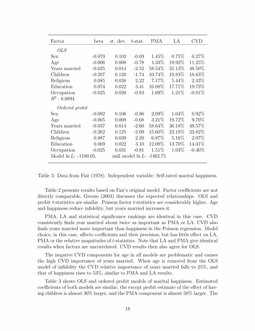
Table 3: Data from Fair (1978). Independent variable: Self-rated marital happiness.

Table 2 presents results based on Fair’s original model. Factor coefficients are notdirectly comparable, Greene (2003) discusses the expected relationships. OLS andprobit t-statistics are similar. Poisson factor t-statistics are considerably higher. Ageand happiness reduce infidelity, but years married increases it.

PMA, LA and statistical significance rankings are identical in this case. CVDconsistently finds year married about twice as important as PMA or LA. CVD alsofinds years married more important than happiness in the Poisson regression. Modelchoice, in this case, affects coefficients and their precision, but has little effect on LA,PMA or the relative magnitudes of t-statistics. Note that LA and PMA give identicalresults when factors are uncorrelated. CVD results then also agree for OLS.

The negative CVD components for age in all models are problematic and causesthe high CVD importance of years married. When age is removed from the OLSmodel of infidelity the CVD relative importance of years married falls to 25%, andthat of happiness rises to 53%, similar to PMA and LA results.

Table 3 shows OLS and ordered probit models of marital happiness. Estimatedcoefficients of both models are similar, the except probit estimate of the effect of hav-ing children is almost 30% larger, and the PMA component is almost 50% larger. The

18

increase in the LA component is just above 15%. Explained variance is proportionalto the square of the beta in uncorrelated OLS, which would imply a 69% increase.

For the OLS and ordered probit models of marital happiness, all attribution meth-ods indicate years married is most important. The bootstrap probability that PMAyears married is larger (more important) than PMA education is greater than 85%. Incontrast, t-statistics seem to show education is most precisely estimated. In practice,this result is commonly interpreted as indicating that education is most important.

Age and years married are highly correlated (ρ = .78), which degrades statisticaltest values. Indeed, when age is excluded the years married t-statistic becomes largest(-4.44 for OLS). Age, however, may be a valid predictor for marital happiness. If so,its exclusion from the model could bias the model and attribute its explanatory powerto the factors with which it is most correlated. Also, the LA for years married rises to51% when age is excluded, indicating the relative sensitivity of LA to model definition.

An F -test of the joint significance of sex and age in the OLS model is rejected(p=0.76). But removing age increases the magnitude of the years married beta by22%. It would be a mistake to exclude age if the goal was to obtained unbiasedcoefficient estimates unless it could be maintained that age did not belong in themodel in the first place. The age PMA of 4.33% signals this result.

4 General microeconomic models

4.1 Inert factors and utility attribution

Is random order consistency an acceptable axiom for utility attribution? Considerthis question in the context of portfolio optimization. Uncorrelated assets, e.g., risk-free assets, are not inert factors: Their utility contribution is not independent of otherassets. Further, an investment option of zero utility cannot be inert by definition.

The ability to define an inert factor must thus rely on a factor that is not aportfolio choice. Its utility must be independent of the portfolio. These conditionsare satisfied if utility is additively separable in the investment and the inert factor.

There is no reason why two completely independent choice problems could not, inprinciple, be composed into a single optimization problem. This simple fact appearsto allow the definition of an inert factor in almost any choice problem. Random orderconsistency becomes applicable once it is established the existing attribution problemcould be composed with a suitable independent problem as a larger attribution.

Proposition 4.1 A factor in an attribution problem is inert if the attribution can beredefined as two independent attributions, one including only this factor.

19

Risk and return CorrelationAsset Mean Std. Sharpe LC SC Intl Gvt Corp BillsLarge Cap 0.0106 0.041 0.258 1.000 0.729 0.619 0.116 0.217 0.069Small Cap 0.0110 0.053 0.209 0.729 1.000 0.529 -0.015 0.110 -0.053Int’l 0.0062 0.048 0.128 0.619 0.529 1.000 0.009 0.082 -0.068LT Gvt. 0.0082 0.026 0.320 0.116 -0.015 0.009 1.000 0.948 0.079LT Corp. 0.0079 0.021 0.384 0.217 0.110 0.082 0.948 1.000 0.069T-Bills 0.0037 0.002 — 0.069 -0.053 -0.068 0.079 0.069 1.000

Table 4: Asset performance data, monthly 1988-2004.

4.2 Portfolio attribution

Let N be a set of n assets with expected return vector µ and covariance matrix Σ.Using quadratic utility and formula (1), v(S) for any set of assets S is

vmvo(S) = U(S)− U(∅) = max(0, maxωS∈∆S

ω′SµS − λω′SΣSωS), (16)

where λ is the index of quadratic risk aversion, µS, ωS and ΣS are restricted to themembers of S, ωS is the portfolio allocation and ∆S is the s− 1 dimensional simplexof nonnegative portfolio weights that sum to unity. Here U(∅) = 0. The restrictionv(S) ≥ 0 allows not investing if v(S) < v(∅), as is possible when restricted to someasset combinations. If exponential utility were used, then U(S) < 0 for all S ⊆ Nand the definition v(S) = U(S)−U(∅) is necessary, as in Section 3.2 for likelihoods.

Table 4 reports the assets used in this example, along with their monthly meantotal returns, standard deviations, Sharpe ratios and correlations for the period 1988to 2004.6,7 Table 5 presents the optimal portfolios for an individual with quadraticrisk aversion level λ = 2, along with two sets of attributions. One is for all investmentoptions. The other excludes corporate bonds. For each set, PMA and LA results and(discrete) marginal utility contributions are reported. All attributions are normalizedto 100%. The final column of Table 5 presents the proportional marginal performanceattribution (PMPA) of assets with positive portfolio allocations. The PMPA of anasset is the ratio of its PMA to its portfolio weight.

6Monthly data from Ibbotson Associates covers the period January 1, 1988 to December 31,2004. Large cap is the S&P 500, small cap is the Russell 2000, international is the MSCI Europe,Asia and Far East Index, long-term government is the Ibbotson U.S. Long-Term Government BondIndex, long-term corporate is the Ibbotson U.S. Long-Term Corporate Bond Index and t-bills is theIbbotson U.S. 30 Day T-Bill.

7The Sharpe ratio is the excess return of an asset over the risk free rate divided by its standarddeviation. The Sharpe ratio is a measure of excess return per unit of risk.

20

Port. With LT Corp. W-out LT Corp.Asset Wts. PMA LA Marg. PMA LA Marg. PMPALarge Cap 37% 49% 25% 55% 49% 31% 19% 1.32Small Cap 17% 7% 17% 19% 7% 21% 6% 0.41Int’l 0% 0% 3% 0% 0% 4% 0% —LT Gvt. 46% 44% 23% 26% 44% 33% 75% 0.96LT Corp. 0% 0% 23% 0% — — — —T-Bills 0% 0% 9% 0% 0% 11% 0% —

Table 5: Asset allocation and performance attribution when λ = 2.

The optimal portfolio monthly return and standard deviation are 0.0096 and 0.026and its Sharpe ratio is 0.364. It is about 54% equity and 46% fixed income. The PMAis in similar proportion (56%/44%). Only assets with positive portfolio weight receivea PMA share, while every asset class receives some LA share. LA gives governmentand corporate bonds almost equal importance even though corporate bonds receiveno portfolio weight. Marginal contributions are heavily weighted to equity becauseof the substitutability of government and corporate bonds.8

PMPA provides a measure of an asset’s per dollar contribution to portfolio per-formance. The PMPA ranking is differs from the Sharpe ratio ranking. Governmentbonds have the highest Sharpe ratio of all allocated assets, followed by large capequity. But Large cap equities contribute most to portfolio performance per unit ofinvestment. The PMPA of large cap equity is more than three times the PMPA ofsmall cap equity even though its Sharpe ratio is only 23% higher. The Sharpe ratiomeasures stand-alone performance, whereas PMPA evaluates performance relative toa specific portfolio. (Note, corporate bonds have the highest Sharpe ratio but receiveno asset allocation.) Further, attribution is relative to a specific risk profile.

In the second set of attributions of Table 5, corporate bonds are not an option. ThePMA does not change. The LA equity share rises to 52%, but now government bondsare seen as more important than large cap equity. The relative marginal contributionof government bonds is now very high without substitution from corporate bonds,and equity marginal contribution is weak because of equity mutual correlation.

If t-bills and international equity are also removed from the choice set, the LAbecomes (37%, 25%, 28%) and equity receives 62% total attribution. PMA resultsare unchanged. When large cap and small cap shares are aggregated, the PMA is(52%, 48%) and the LA is (53%, 47%). In all cases, PMA implies that a little over

8The Covariance decomposition is (83%, 59%, -42%) to the three allocated assets. Only portfolioassets receive non-zero CVD allocations. CVD is based on portfolio weights and Σ (see footnote4) and is commonly used in portfolio analysis. A marginal increase in government bonds reducesportfolio risk. This is the essential meaning of the negative CVD coefficient. CVD weights marginalrisks by portfolio weights. Long term bonds, however, clearly both contribute to risk and utility.

21

half of portfolio performance is attributable to equity and almost half to bonds. LAimplications depend strongly on details of the attribution analysis.

Unutilized assets are irrelevant for PMA because of exclusion. In this example,and generally, PMA is not very sensitive to aggregation; but it is possible to constructcontrary examples. Linear attribution is sensitive to both unutilized factors and factoraggregation (as in example 5.1, below). The differences between LA and PMA maybe a useful measure of the substitutability of factors. PMA offers a consistent methodof attributing joint effects in the creation of investment value, and thereby providinginsight into its sources.

5 Joint cost attribution

Cost allocation has traditionally been considered a bargaining problem by game the-orists. In cost attribution, the utility function of formula (1) is an aggregate cost(disutility) function. The arguments of the cost function are typically aggregate de-mands for products or services over cost centers. The applicability of random orderconsistency to cost attribution raises the same types of issues as considered for utilityattribution in Section 4.1. The potential existence of an inert cost center is no differ-ent the potential existence of an inert factor in a utility or econometric attribution.

5.1 Linear or proportional marginal cost attribution?

Neither inclusion nor exclusion appear obviously appropriate for cost attribution.While exclusion might seem appropriate for the attribution of profits, many mightfind it problematic that somebody is getting something for nothing. Exclusion in costallocation requires that a party that imposes no final marginal cost should have noattributed cost if all other parties impose final marginal costs.

Inclusion may appear an innocuous axiom in this context, however linear costallocation methods have not been widely adopted and were not well-received by ac-counting researchers. Moriarity (1975), Banker (1981) and Gangolly (1981) explicitlysupport or propose proportional alternatives. Banker writes that linear attribution is“not consistent with our axioms, and hence with traditional cost allocation methods.”(1981:127). Thomas (1977) provides examples that demonstrate the vulnerability oflinear attribution to strategic definition of cost centers.9

Example 5.1 The potential for strategic manipulation in cost attribution is illus-trated in a simple sunk cost attribution problem. Assume n cost centers, sunk costC and fixed marginal cost c. Cost center i has usage xi. The cost of service to any

9Note also the conference proceedings Moriarity (1981). See Feldman (1999), Section 9.2, formore on accountant’s perspectives.

22

coalition of centers S is v(S) = C + c∑

i∈S xi. The marginal cost of any coalition ofcenters S 6= N , is represented in the dual game by w(S) = c

∑i∈S xi. Thus, the game

w(S) is additive for all S ( N : w(S) =∑

i∈S w(i ).

Lemma 2.2 implies PMAi = ϕ(w)i = C/xi because w can seen as a rescaling ofw∗(N) in a w∗ where w∗(N) = c

∑i∈N xi. Similarly, LAi = cxi + C/n. When C is

very small, LA and PMA are approximately the same since then v(N) ≈ c∑

i∈N xi.However, allocations diverge as C increases. When c

∑i∈N xi ¿ C, LA for all

centers approaches C/n, regardless of the disparities in usage between cost centers,providing incentive for group managers to aggregate reporting units.

Corollary 5.1 The proportional marginal share of costs attributed to any cost centeris invariant with the magnitude of the fixed costs when fixed costs are scale invariant.

6 Discussion and conclusion

This paper introduces a new expectation-based random order approach to cooperativevalue. Linear and proportional value are characterized in a common setting withoutassuming linearity or proportionality. Random order consistency, the key elementof this approach, assumes only that we can see the “expectational mechanics” ofthe random order process, and that these mechanics do not change if invisible inertplayers or factors are added. These mechanics have specific interpretation regardingthe relative importance of factors in the theory of attribution developed here.

Random order consistency is key to both theoretical and applied results. Contrastthis with the limited power of reduced game consistency discussed in Remark 1.1.Random order consistency is strongly and uniquely associated with cooperative value.

Consider the scope of this theory if based on reduced game consistency. The use ofreduced game consistency must imply some correspondence between the reduced gameand the original attribution. But few, if any, properties of a game or cost function arepreserved by reduction. The reliance on the dual game is also problematic. Consideran attribution problem with a vector of demands x and cost function c(y) = yα, α 6= 1,so w(S) = c(xN)− c(xN\S) = [

∑i∈N xi]

α − [∑

i∈S xi]α. Let w∗ be the game resulting

from the reduction of player k, so that N∗ = N \ k and w∗(S) = w(S ∪ k) − φk(w),where φi(w) is Shi(w) or ϕi(w). In general, there will be no vector of demands x∗

such that w∗(S) = c(x∗N∗) − c(x∗N∗\S) for all S. Nor, in general, will there be a cost

function c∗ such that w∗(S) = c∗(x∗N∗)− c∗(x∗N∗\S) for all S.10

Random order consistency places minimal demands on the structure of an attri-bution problem. Section 4.1 proposes it appropriate for any attribution problem thatcan be composed with an independent attribution.

10Compare this perspective on the reduced game with Dubey’s (1982) discussion regarding thethe benefits of a direct characterization of a cost allocation problem based on its specific features.

23

The specific applications studied here demonstrate practical potential applica-tions. PMA appears to provide theoretically sound measures of the econometricrelative importance of model independent variables. These measures also appear toallow comparison of relative importance across models and to be useful diagnosticsfor model construction and evaluation. Feldman (2005a and 2006) applies a similarapproach with financial factor models to provide variance decomposition of an assetmanager’s return stream to identify the relative importance of factor drivers.

The portfolio attribution example shows the considerable knowledge of data andpreferences necessary for utility attribution, but, also, the potential benefit. PortfolioPMA and PMPA are new investment analysis tools and examples of practical feasibleapplications. They are distinctive in that they evaluate an asset’s total, as opposed tomarginal, performance both relative to a portfolio and an investor’s risk preferences.

In this theory of attribution, linear and proportional value emerge as parallelexpressions of an underlying value principle. This relative importance approach tocooperative value is developed specifically for the single-utility function attributionenvironment, but applies directly to TU bargaining as well. Feldman (2002) developssimilar results for the more general nontransferable utility (NTU) games using ratiopotentials. In this “dual” approach to value either the linear or proportional “mode”might be more appropriate for a particular application.

Game theoretic interest in proportional solutions, including the proportional value,has been hampered by the belief that they are translation dependent (see, e.g., Hartand Mas-Colell (1988: 595n)). Real allocations seem to change with affine translationof a player’s utility function. This outcome should arouse scrutiny as it implies theincoherence of a basic distributive principle recognized at least since Aristotle.11

The apparent translation dependence of proportional solutions results from a miss-ing element in the standard NTU cooperative game. The basis point, a vector of util-ities, one for each player, allows determination of the marginal utility to any playerof any bargaining outcome. Feldman (2005b) demonstrates the existence of the basispoint and shows that proportional solutions are translation invariant when a player’sbasis utility and utility function are subjected to the same affine transformation.12

This theory of attribution is based on a single decision maker and, hence, wouldbe unaffected even if proportional bargaining solutions were translation dependent.Examples presented here clearly demonstrate the relevance of the basis point in at-tribution problems. Section 3.2 shows that econometric attributions are not uniquelydefined unless the null model objective function value can be defined and used asthe basis point. (Interestingly, PMA shares are invariant to the choice of the basispoint.) Similarly, Section 4.2 shows that utility attribution must specifically definenull model utility for utility functions where null model utility is not zero.

11Young (1994: 64) writes “[p]roportionality is deeply rooted in law and custom as a norm ofdistributed justice.” Moulin (1999) starts by quoting Aristotle: “Equals should be treated equally,and unequals, unequally in proportion to relevant similarities and differences.”

12Recognition of the basis point implies intrapersonal but not interpersonal comparison of utility.

24

Finally, researching the accounting literature, I was often surprised by the inten-sity of the arguments against linear cost allocation, and sometimes by the palpablefrustration. Thomas (1977: 43), in his study of cost allocation and transfer pricing,chooses the following epigraph (from Lousia M. Alcott’s Jack and Jill) for his chapteron cost allocation using the Shapley value: “. . .Molly retired to wet her pillow witha few remorseful tears, and to fall asleep, wondering if real missionaries ever killedtheir pupils in the process of conversion.” Neutrality between linear and proportionalmethods is theoretically sound and evolutionarily wise.

7 Proofs

7.1 Appendix A: Proof of Lemma 1.1

Proof: I. First consider multiplicative likelihoods. Endogenous random order con-sistency requires that functions of the worths of factor sets including an inert fac-tor factor out of the sum of likelihoods generated by a suborder. The terms in∑

r⊃ro

∏i∈N li(w(Sr

i )) do not factor directly. An alternate approach is required.

Consider a single inert factor z ∈ N . Select any r0 in R(N \ z). By insert-ing z at all possible positions in r0, all orders in N that include r0 are generated.Define ri

0 ∈ R(N) as the order resulting when z is inserted at the ith position:ri0 = (r01 , . . . , r0i−1

, z, r0i, . . . , r0n−1). Then let R∗ = ri

0ni=1 = (r1

0, r20, . . . , r

n0 ).

Define S as all nonempty factor sets included in r0, so that S = S : S ⊂ r0 =Sr0

i n−1i=1 . Let Sz contain the singleton z and the union of each factor set in S with

z: Sz = S : S = T ∪ z, T ∈ S or T = ∅. Index the members of S and Sz by theircardinality: S3 has cardinality three. Define S∗ = S ∪ Sz.

Set of sets S∗ helps to form a common denominator for multiplicative likelihoods.For any ri

0 ∈ R∗, let R∗i be the factor sets that are included in ri

0: R∗i = S |S ∈ ri

0.R∗

i ⊂ S∗. Define T ∗i as the sets in S∗ not included in ri

0: T ∗i = S∗ \ R∗

i . LetK =

∏S∈S∗ li(S)−1, where i is the cardinality of S. Then, for all i ∈ N ,

L(ri0) =

∏

S∈ri0

li(S) =1

K

∏

S∈T ∗i

li(S)−1 ≡ 1

KL(ri

0), (A1)

where L is a partial likelihood with Li = l−1i . For every j < n there are two sets in

S∗ with j factors. Only one of these factor sets is in any T ∗i . These are Sro

j = Sj

and Szj = Sro

j−1 ∪ z. If one is in R∗i then it is not in T ∗

i , and vice-versa. For j < i,Sz

j ∈ T ∗i because Sj ∈ R∗, and for j ≥ i, Sj ∈ T ∗

i because Szj ∈ R∗. Thus, T ∗

i =

Szi−1j=1 ∪ Sn−1

j=i . Note Szn = N ∈ R∗

i and N 6∈ T ∗i .

25

Let T ∗ij be the factor set in T ∗

j of cardinality i. Then

L(r10) + L(r2

0) =n−1∏i=1

li(T∗i1 )−1 +

n−1∏i=1

li(T∗i2 )−1

=(l1(S

z1)−1 + l1(S1)

−1) n−1∏

i=2

li(Si)−1.

When w(Sz1) = w(z) > 0 factorization requires l1(S) = l2(S) = w(S)−1. Then

l(S)−1 = w(S) and, since z is inert, w(Sz2) = w(z) + w(S1). Note that any l with

l(0) = ∞ trivially allows factorization if w(z) = 0. (Thus the requirement that inertfactors have positive individual worth.) If and only if l1(S) = l2(S) = w(S)−1 canthese terms be combined and absorbed into the product

L(r10) + L(r2

0) = w(Sz2)

n−1∏i=2

li(Si)−1.

Induction is used to sum likelihoods. Assume that li(S) = w(S)−1 for all i < jand that the following pattern holds for sums of the first j − 1 orders in R∗:

j−1∑i=1

L(ri0) =

j−1∏i=2

w(Szi )

n−1∏i=j−1

li(Si)−1.

Under the above assumptions, L(rj0) may be written

L(rj0) =

j−1∏i=1

w(Szi )

n−1∏i=j

li(Si)−1.

Adding and factoring the last two expressions gives the first formula below. Thesecond follows if and only if lj(S) = w(S)−1. The induction is a “zipper.”

j∑i=1

L(ri0) =

(w(Sz

1) + w(Sj−1)) j−1∏

i=2

w(Szi )

n−1∏i=j

li(Si)−1

=

j∏i=2

w(Szi )

n−1∏i=j

li(Si)−1 (A2)

Evaluating (A2) at j = n and recalling (A1) and that S = S : S ∈ ro gives

1

K

n∑i=1

L(ri0) =

1

K

n−1∏i=2

w(Szi ) = w(z)−1

∏S∈r0

w(S)−1 = w(z)−1L¦(r0).

26

The sum of likelihoods generated by an r∗0 ∈ R(N) divided by those generatedby r0 thus equals L¦(r∗0)/L

¦(r0), proving p¦(r0|w0) =∑

ri0⊃r0

p¦(ri0|w), where w0 is

the dual game generated by N \ z and p¦ is the distribution induced by L¦. Thus,L¦ is random order consistent between games of cardinality n − 1 and n for anyn > 2. Consistency between games of cardinality m > 2 and n is established byrepeat reduction of individual inert factors. L¦ is random order consistent.

Any L′ = c L¦, where c > 0, is also random order consistent, but still generatesp¦. An L′ created by dropping any li or combination of li is not random orderconsistent because the zipper will fail. The only way that the terms that depend onall Sz can be factored out of the sum

∑r⊃r0

L(r) is by combining terms using therelationship li(Si) + l1(S

z1) = li+1(S

zi+1), possible because z is inert. This restricts li

to li(Sri ) = w(Sr

i ) or li(Sri ) = w(Sr

i )−1. Using the terms in L¦ directly (as opposed

to L¦) allows combination when li(Sri ) = w(Sr

i ), but combination is only possiblebetween r1

0 and r20. There are no other endogenous, nontrivially different l′in

i=1 thatsimultaneously allow combination of terms and addition of likelihoods. For example,with l′i = w(Sr

i )2, l′i(Si)

12 + l′1(S

z1)

12 = l′i+1(S

zi+1)

12 , but combining on this basis implies

L′(r0)12 =

∑r⊃r0

L′(r)12 . Thus, L¦ is unique up to scaling.

L¦ is endogenous and multiplicatively separable. L¦ is anonymous. Non-anonymousvariants cannot be random order consistent because distinguishing orders will causethe zipper to fail. Finally, L¦ is clearly positive when v is strongly monotonic.

II. Now consider additively separable endogenous likelihoods. Additive separabil-ity allows the collection and regrouping of sublikelihood functions, yielding

∑r⊃r0

L(r) = L(r0) +n−1∑i=1

(n− i− 1) li(Si) +n∑

i=1

i li(Szi ).

Consider two orders r0 and r∗0 in R(N \ z) and the ratio∑

r⊃r∗0L(r)/

∑r⊃r0

L(r).

This ratio must equal L(r∗0)/L(r0) if L is random order consistent. This implies

L(r∗0)L(r0)

=

∑n−1i=1 (n− i− 1) li(Si(r

∗0)) +

∑ni=1 i li(S

zi (r

∗0))∑n−1

i=1 (n− i− 1) li(Si(r0)) +∑n

i=1 i li(Szi (r0))

,

where the dependence on orders is indicated to avoid ambiguity. No further factor-ization of terms involving z is possible. Thus, this equality can hold for arbitrary vonly when li(S

zi (r0)) = li(S

zi (r

∗0)) for all i, i.e., when L is exogenous. ¤

7.2 Appendix B: Proof of Lemma 1.4

Proof: Select any r ∈ R(N \ i) and let rj ∈ R(N), j = 1, . . . , n be the order createdby inserting i at position j, so that rj

j = i. If L¦(r) =∑n

j=1 L¦(rj)mPrj(i)(r

j), the result

27

follows. The key to this reduction is more apparent when mPrj(i)(r

j) is represented

as w(Sjj ) − w(Sj

j−1). The sum can then be expanded into 2n − 1 separate terms.Consider first the order n term, where w(Sn

n) = w(N) is the numerator and also inthe denominator. This term simplifies to L¦(r), the LHS value. Now pair terms fororders rj and rj−1, for every j = 1, . . . , n, and the following equality results:

w(Sj−1j−1)

w(Sj−11 ) · · ·w(Sj−1

j−1) · · ·w(Sj−1n )

+−w(Sj

j−1)

w(Sj1) · · ·w(Sj

j−1) · · ·w(Sjn)

= 0.

First, for all k 6= j − 1, w(Sj−1k ) = w(Sj

k) since i has either not yet entered or hasalready entered both Sj

k and Sj−1k . Then, for position j − 1, where Sj−1

j−1 6= Sjj−1, here

w(Sj−1j−1) and w(Sj

j−1) are each on the top and bottom and cancel. ¤

8 References

Aumann, Robert J. and Lloyd Shapley (1974): Values of non-atomic games. Prince-ton: Princeton University Press.Banker, R. D. (1981): “Equity considerations in traditional full cost allocation practices:An axiomatic perspective,” in Moriarity (1981), 110-130.Billera, L. J. and D. C. Heath (1982): “Allocation of shared cost: A set of axiomsyielding a unique procedure,” Mathematics of Operations Research, 7:32-39.Calvo, Emilio and Theo H. S. Driessen (2003): The multiplicative value in cooperativeTU-games, Working paper, Department of Economic Analysis, University of Valencia.Chevan, Albert and Michael Sutherland (1991): “Hierarchical partitioning,” TheAmerican Statistician, 45:90-96.Dubey, Pradeep (1982): “The Shapley value as aircraft landing fees-revisited,” Manage-ment Science, 28:869-874.Fair, Ray (1978): A Theory of extramarital affairs, Journal of Political Economy, 86:45-61.Feldman, Barry (1999): The proportional value of a cooperative game, netec.mcc.ac.uk/WoPEc/data/Papers/ecmwc20001140.html.

(2002): A dual theory of cooperative value, papers.ssrn.com/abstract=317284.(2005a): Relative importance and value, working paper, www.prismanalytics.com/

docs/RelativeImportance.pdf.(2005b): Lost in translation: Basis utility and proportionality in games, papers.

ssrn.com/abstract=764004.(2006): “Using PMVD to understand hedge fund performance drivers,” in Portfolio

Analysis: Advanced Topics in Performance Measurement, Risk and Attribution, TimothyRyan (ed.), London: Risk Books.Firth, David (1998): Relative importance of explanatory variables, prepared for Statistical

28

Issues in the Social Sciences, Stockholm, October 1998, Oxford: Nuffield College, www.nuff.ox.ac.uk/sociology/alcd/relimp.pdf.Friedman, Eric J. (2004) “Paths and consistency in additive cost sharing,” InternationalJournal of Game Theory, 32:501-518.Gangolly, Jagdish S. (1981): “On joint cost allocation: Independent cost proportionalscheme (ICPS) and its properties,” Journal of Accounting Research, 19:299-312.Greene, William (2003): Econometric Analysis, 5th ed., Prentice Hall.Gromping, Ulrike (2006): “Relative importance for linear regression in R: The packagerelaimpo,” Journal of Statistical Software, 17(1), jstatsoft.org/v17/i01/v17i01.pdf.

(2007): “Estimators of relative importance in linear regression based on variance de-composition,” American Statistician, forthcoming, www.tfh-berlin.de/∼groemp/downloads/amstat preprint.pdf

Gul, Faruk (1989): “Bargaining foundations of the Shapley value,” Econometrica, 57:81-95.Hart, Sergiu (2006): “Shapley value,” in The New Palgrave: A Dictionary of Economics,2nd Edition, Steven N. Durlauf and Lawrence E. Blume, eds., Palgrave MacMillan, forth-coming. (www.ma.huji.ac.il/∼hart/abs/val-palg2.html)

and Andreu Mas-Colell (1989): “Potential, value and consistency,” Economet-rica, 57:589-614.

and (1996): “Bargaining and value,” Econometrica, 64:357-380.Hoffman, P. J. (1960):, “The paramorphic representation of clinical judgment,” Psycho-logical Bulletin, 57:116-131.Kalai, Ehud and Dov Samet (1987): “On weighted Shapley values,” InternationalJournal of Game Theory, 16:205-222.Khmelnitskya, Anna B. (1999): “Marginalist and efficient values for TU games,” Math-ematical Social Sciences, 38:45-54.

and Theo S. H. Driessen (2001): “Semiproportional values for TU games,” Math-ematical Methods of Operations Research, 53:495-511.Kruskal, William H. (1987): “Relative importance by averaging over orderings,” Amer-ican Statistician, 41:6-10.Leroux, Justin (2006): A discussion of the consistency axiom in cost allocation problems,HEC Montreal, Institut D’economie Appliquee working paper IEA-06-13.Lindeman, Richard. H., Peter F. Merenda, and Ruth Z. Gold (1980): Introductionto Bivariate and Multivariate Analysis, Scott Foresman, Glenview, IL.Maddala, G. S. (1983) Limited-Dependent and Qualitative Variables in Econometrics,Cambridge: Cambridge University Press.McNally, Ralph (2000): “Regression and model-building in conservation biology, bio-geography and ecology: The distinction between and reconciliation of predictive andexplanatory models,” Biodiversity and Conservation, 9:655-671.Moriarity, Shane (1975): “Another approach to allocating joint costs.” The AccountingReview, pp. 791-95.

, ed. (1981): Joint Cost Allocations: Proceedings of the University of Oklahoma

29

Conference on Cost Allocations, April 23-24, 1981. Norman: Center for Economic andManagement Research.Moulin, Herve (1999): “Axiomatic cost and surplus-sharing,” Chapter 6 in the Handbookof Social Choice and Welfare, Kenneth J. Arrow, Amartya K. Sen, and Kotaro Suzumura,eds. Amsterdam: Elsevier.

and Scott Shenker (1992): “Serial cost sharing,” Econometrica, 65:1009-37.Myerson, Roger (1980): “Conference structures and fair allocation rules,” InternationalJournal of Game Theory, 9:169-82.Ortmann, K. M. (2000): “The proportional value for positive cooperative games,” Math-ematical Methods of Operations Research, 51:235-48.Owen, Guillermo (1977): “Values of games with a priori unions,” in Essays in Mathe-matical Economics and Game Theory, R. Hein and O. Moeschlin, eds., pp. 76-88, Berlin:Springer-Verlag.Roth, Alvin, ed. (1988) The Shapley Value: Essays in Honor of Lloyd Shapley, Cam-bridge: Cambridge University Press.Schmeidler, David (1969): “The nucleolus of a characteristic function game,” SIAMJournal of Applied Mathematics, 17:1163-1170.Shapley, Lloyd S. (1953): “A value for n-person games,” in Contributions to the Theoryof Games, Vol. II, eds. H.W. Kuhn and A.W. Tucker, Princeton University Press, 307-317.

(1964): “Values of large games VII: A general exchange economy with money,” RANDRM 4248-PR.Shubik, Martin (1982): “Incentives, decentralized control, the assignment of joint costsand internal pricing,” Management Science, 8:325-343.Soofi, Ehsan S., Joseph J. Retzer, and Masoud Yasai-Ardekani (2000): “A frame-work for measuring importance of variables with application to management research anddecision models,” Decision Sciences 31:1-31.Thomas, Arthur L. (1977): A Behavioral Analysis of Joint-Cost Allocation and TransferPricing, Chicago: Arthur Andersen & Co.von Neumann, John (1928/1959): “On the theory of playing games,” English transla-tion in Contributions to the Theory of Games IV, ed. by R. D. Luce and A. W. Tucker.Princeton, Princeton University Press, pp. 13-42.Weber, Robert J. (1998): “Probabilistic values for games,” in Roth (1988), pp. 101-119.Young, H. Peyton (ed.) (1985): Cost Allocation: Methods, Principles, Applications,Amsterdam: North-Holland.

(1994): Equity: In Theory and Practice. Princeton: Princeton University Press.

30