SYSTEMS TECHNOLOGY, INC.CInglewood, Califor n i a

TECHNICAL REPORT NO. 124-1

A SYSTEMS ANALYSIS OF LONGITUDINAL PILOTED CONTROL

IN CARRIER APPROACH

"BY-;• C.H. CROMWELL

I. L. ASHKENAS

ct '

JUNE 1962

U PERFORMED UNDER

CONTRACT NO. NOw 61-0519-c

FOR

BUREAU OF NAVAL WEAPONS

DEPARTMENT OF THE NAVY

WASHINGTON, D. C.

TECHNICAL REPORT NO. i24-I

A SYSTEMS ANALYSIS OF LONGITUDINAL PILOTED CONTROL IN CARRIER APPROACH

(Final Report)

C. H. CromwellI. L. Ashkenas

June 1962

Performed underContract No. NOw 61-0.519-c

forBureau of Naval WeaponsDepartment of the Navy

Washington, D. C.

if

This report covers the first, and analytical, phase of a program to

investigate piloting problems of carrier approach using systems analysis

methods to attack the problem. The research was sponsored by the

Airframe Design Division of the Bureau of Naval Weapons under Contract

NOw 61-0519-c. Mr. C. H. Cromwell served as project engineer, and

Mr. Harold Andrews served as technical monitor for the Bureau of Naval

Weapons.

Special mention is due to Mr. Tulvio Durand for his contributions to

the technical appendices of the final report, and to R. N. Nye and

D. Lewis for their careful work in preparing the manuscript.

ABOOACT

The pilot's longitudinal control of an aircraft making a carrierapproach is studied using systems analysis techniques. The pilot,

airframe, and mirror optical landing aid are considered as elements

in a closed-loop system. Mathematical expressions to approximate each

element are derived or described. Various possible piloting techniques

are examined by appropriately varying the pilot's transfer function,

and by closing multiple control loops around the system. The question

of whether the pilot should use stick or throttle for altitude control

is examined. It is shown that the minimum approach speeds of five out

of seven jet aircraft, all limited by the "ability to control altitude

and arrest rate of sink," can be predicted if it is assumed that the

pilot uses throttle for altitude control.

CONTENTS

I INTRODUCTION .......... . I

A. Background of the Report .... ..... ... I

B. Scope of the Report. . ....... . . . 3

C. Outline of the Report .............. ....... 4

II SYSTEM ASPECTS OF CARRIER APPROACH ..... ....... .. 5

A. The System ......... ....... . ...... 5

B. Transfer Functions of the System Elements . . . 7

III CLOSED-LOOP CHARACTERISTICS OF POSSIBLE PILOTING TECHNIQUES. 13

A. Pilot Closure of the e o be Loop. ........... 14

B. Altitude Control with Elevator (h -* Be, e be, ,u or m-> 6T).............. 15

C. Altitude Control with Throttle (h -4- BT, e -b e.,

u or m--> be) ......................... 18

D. Altitude Control with Elevator and Throttle(h --> be, P T; e -- be; u or m --> Be, BT) 19

E. Pilot Opinion Considerations ............... 20

IV A MINIMUM APPROACH SPEED CRITERION DERIVED FROMSIMPLIFIED MULTIPLE-LOOP CONSIDERATIONS ... ....... 22

A. Derivation of the Criterion .... ....... .. 22

B. Testing the Criterion: Agreement BetweenPredictions and Flight Test Minimum ApproachSpeeds ................ ........ .. 31

V SUMMARY AND CONCLUSIONS ................ ..... 34

REFERENCES ......... ...... .................. 38

APPENDIX A - DERIVATION AND SUMMARY OF TRANSFER FUNCTIONS FORBOTH SINGLE-LOOP AND MULTIPLE-LOOP CONTROL 40

APPENDIX B - GENERIC PROPERTIES OF SINGLE- AND MULTIPLE-LOOPFEEDBACK CONTROLS. . ......... . . .. 50

APPENDIX C - A DETAILED EXAMPLE OF THE ANALYSIS TECHNIQUE. . . . 70

iv

FIOURM

1 Geometry of the Aircraft-Mirror-Carrier ysytem ..... 5

2 Multiple Loop Feedback Control System Block Diagram . . . 6

3 Root Locus Illustration of Successive Loop Closures . . . 27

4 Criterion Versus Approach Speed .... .......... . 33

B-1 Attitude Control by Pilot ...... ............ 52

B-2 Sip. Bode Plot (a - -a) of the Phugoid Modefor Various Values of 1/Te . . . . .. . . . . . . . . . . . 54

B-3 h -B be Control by Pilot ....... ............ 55

B-4 h -- loT; Front and Back Side of the Drag Curve ....... 56

B-5 Effect of Thrust Line Offset on h --> 8T Zeros ..... 58

B-6 Speed Control Loops .......... .............. 59

B-7 Effect of Thrust Offset on u -) 5T Zeros .. ....... 60

B-8 Angle of Attack Control Loops ........ ........... 61B-9 Pilot Closure of the u -o BT Loop ....... ... .. ..• . 63

B-1O Effect of u -0. 8T on h --> e Zeros ...... ......... 64

B-11 Altitude Control with Elevator ..... .......... 66

B-12 u-3 BT Closed Outer Loop .......... ............ 67

B-1 3 c,-- 5T Closed Outer Loop ...... ........... 67

B-14 h -* bTp Final Closure ........ ............. 68

B-15 s-Plane Representation of Closed u -) be Outer Loop . . . 69

C-I Closure of the Piloted 0 -I- beLoope ..... ......... 73

C-2 Factorization of Nue +uYeNe ............. 75

C-3 Closure to Effect Stabilization of the Altitude Control Zero 77

C-4 Effect of the Speed Control Loop Closure onthe Altitude Control Denominator ........ .......... 79

v

Pago

C-5 Altitude Control vith 0 - b e., u -- 8T Inner Loops Closed 81

C-6 Effect of the Altitude Control Loop Closure onthe Airspeed Control Numerator .......... 83

C-7 9 -* be, h -i be Inner Loop Effects on AirspeedOpen-Loop Denominator (Eq C-9) . . . . . . . . .. 84

* C-8 Effect of a -) 5T on Altitude Control Zeros ...... . 86

Page

I Summary of Predominant Loop-Closure Effects .. ...... .. 20

II Comparison of Criterion-Predicted Minimum Approach Speedand Flight Test Speed(s) ............

A-1 Transfer Function Coefficients and Factored Forms ... .

A-2 Longitudinal Coupling Numerator Coefficients andFactored Forms ............. ................ 48

C-i Characteristics of the FAD-1 at 120 Knots, vith • 0 71

vi

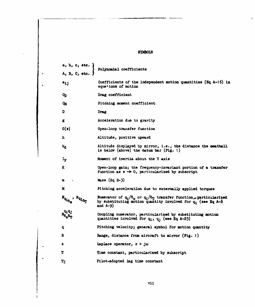
SYMBOLS

a A, as C, o. I Polynomial coefficientsAs B: C, Zt.

aia Coefficients of the independent motion quantities (Eq A-16) inequations of motion

CD Drag coefficient

CK Pitching moment coefficient

D Drag

g Acceleration due to gravity

G(s) Open-loop transfer function

h Altitude, positive upward

hd Altitude displayed by mirror, i.e., the distance the meatballis below (above) the datum bar (Fig. 1)

Iy Moment of inertia about the Y axis

K Open-loop gain; the frequency-invariant portion of a transfer

function as s -0- 0, particularized by subscript

m Mass (Eq B-3)

M Pitching acceleration due to externally applied torques

Nq be, NqiaT Numerator of qi/be or qi/ST transfer function, particularizedby substituting motion quantity involved for qi (see Eq A-8and A-9)

Nq•_ qCoupling numerator, particularized by substituting motionN508T quantities involved for qij, qj (see Eq A-23)

q Pitching velocity; general symbol for motion quantity

R Range, distance from aircraft to mirror (Fig. 1)

s Laplace operator, a + jw

T Time constant, particularized by subscript

TI Pilot-adopted lag time constant

vii

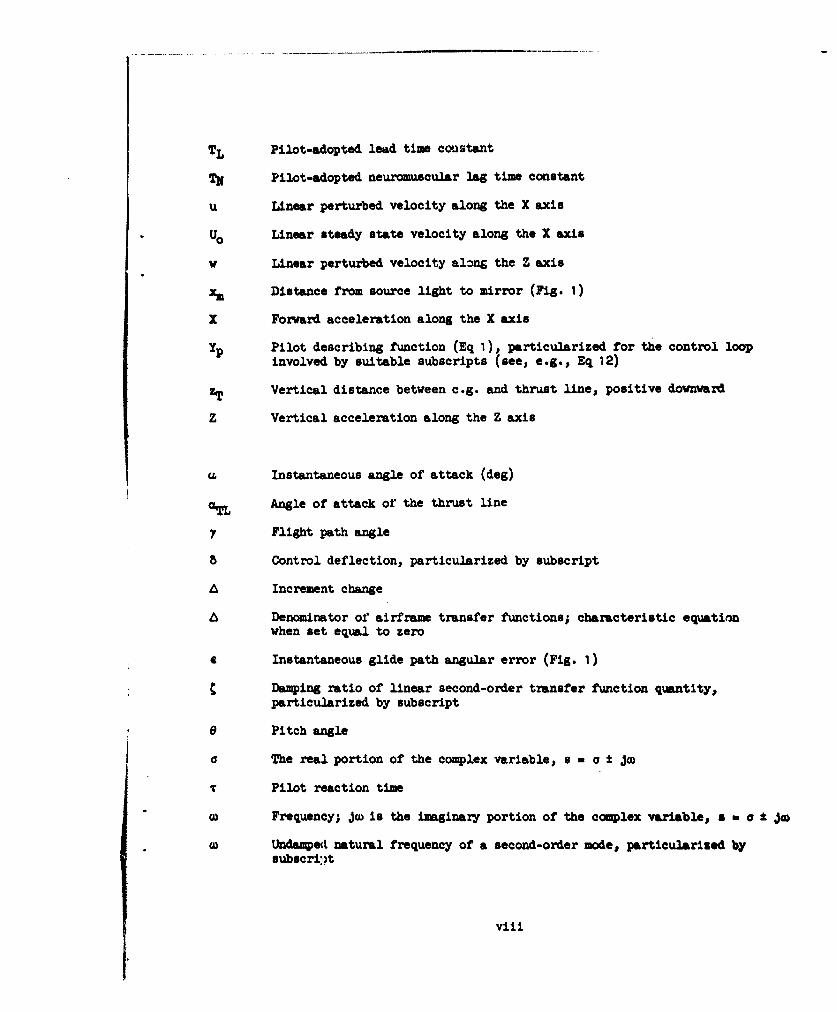
TL Pilot-adopted lead time constant

TN Pilot-adopted neuromuscular lag time constant

U Linear perturbed velocity along the X axis

Uo Linear steady state velocity along the X axis

w Linear perturbed velocity along the Z axis

XM Distance from source light to mirror (Fig. 1)

X Forward acceleration along the X axis

Yp Pilot describing function (Eq 1), particularized for the control loopinvolved by suitable subscripts (see, e.g., Eq 12)

ZT Vertical distance between c.g. and thrust line, positive downward

Z Vertical acceleration along the Z axis

Q Instantaneous angle of attack (deg)

uTL Angle of attack of the thrust line

Y Flight path angle

8 Control deflection, particularized by subscript

a Increment change

. Denominator of airframe transfer functions; characteristic equationwhen set equal to zero

4 Instantaneous glide path angular error (Fig. 1)

* Damping ratio of linear second-order transfer function quantity,particularized by subscript

e Pitch angle

a The real portion of the complex variable, s - a ± 3w

T Pilot reaction time

SFrequency; jw is the imaginary portion of the complex variable, a - I j ow

W Undamped natural frequency of a second-order modej particularized bysubscript

viii

Subscripts

e Comand; controlled element (vehicle)

CL Closed loop

* Elevator, as in be

a Incremental error

m kirror

min Minimum

p Pilot, as in bp for pilot's controlled deflection

p Phugoid

sp Short period

T Throttle, as in BT

h

9 Pertaining to control of the variable indicatec, as in Ag, , etc.

u

be

5T Indicates partial derivative, e.g., M. - •, ZT -q37U

V

Note: Primes on a transfer function or time constant indicate that it hasbeen modified by inner-loop closures, the number of primes corre-sponding to the number of closures.

ix

SZOI 1XVON

A. - MROM•F 0 = RVORT

As new generations of high performance carrier-based aircraft are designed

and introduced into fleet operation, the carrier-landing approach speed

increases. These speeds are reaching the point of arresting gear limits, are

posing aircraft structure design problems, and are causing piloting problems

attributed to fast closure rates between aircraft and carrier. The remedy to

all of these problems is simply to reduce approach speeds, yet the effect of

modern design trends has been to increase them.

As speeds increase it also becomes more important to predict at the design

stage what the eventual pilot-selected approach condition will be, and thisrequires an appreciation of the factors that cause the pilot to set his mini-

mum allowable value. Early attempts at predicting approach speeds simply

chose a fixed margin above the power-on stall speed, usually about 15 percent.

With the advent of sweptwing jet aircraft it was soon found that this simple

criterion was no longer adequate and more elaborate methods were devised.

Pilots were complaining of problems in controlling the aircraft, both longi-

.tudinally and laterally, so the second ger ration of approach speed criteria

considered the ability of the aircraft tu maneuver, usually in response to

discrete step-type control inputs (e.g., Ref. 1). Criteria based on this

concept have enjoyed only limited success in predicting approach speeds and

have not led to a real understanding of the piloting problems because they do

nct realistically consider the pilot's role in control of the aircraft.

A fundamentally different approach to the problem is used in this report.

The pilot, his aircraft, and the mirror display are regarded as elements of a

closed-loop feedback control system. The pilot is assumed to perform the

same role as an autopilot In an automatic landing system; that is, he compareswhat the aircraft is doing with what he wants it to do and he actuates the

controls in response to the errors that he observes in altitude, airspeed,

etc. Thus he performs the sensor-actuator function of the autopilot. The

analytical method, using this concept, employs the well-developed mathematical

techniques of servo system analysis which are used to study any automatic

flight control system. The evaluation process at any given approach speed(and therefore fixed vehicle dynamics) consists of making a series of loop

closures while varying the pilot's mathematical "autopilot" characteristics.When a near-optimum closed-loop system has been obtained the results arejudged by two criteria: First, is the closed-loop performance, as a tracking

system, adequate for the assigned task (in this case to successfully complete

the approach to a carrier landing)? Second, does attainment of that system

performance require too much dynamic equalization from the pilot? (This

latter point refers to the adaptive capability of the pilot and whether this

capability is being exceeded or not.)

As approach speed is lowered and the aircraft's dynamic characteristics

change, some speed is found below which these criteria can no longer be

satisfied. This is predicted to be the minimum acceptable approach speed.

The cause of the limitation is connected with airframe dynamics, defined in

the terms used in control systems analysis (i.e., frequencies, damping ratios,

etc.). However a knowledge of the relationship between these airframe trans-

fer function parameters and their associated aerodynamic stability derivative&

(i.e., approximate factors of the transfer functions in terms of stability

derivatives, as given in Ref. 2) allows the approach speed limit to be related

to the aircraft's basic aerodynamics. The net result of the investigation is

therefore the same as with other prediction methods: aerodynamic characteris-

tics are correlated with the minimum approach speed. It is only the analytical

concept of treating the problem as a closed-loop system problem which differs

from previous methods.

The treatment of handling qualities problems by servo analysis techniques

has been a slowly evolving process. Early programs were aimed at measuringand analyzing the dynamic characteristics of the human pilot (i.e., his

"transfer function"); much of this work up to 1956 is sunmarized in Ref. 3.Lateral and longitudinal attitude control, using the mathematical model of

the pilot determined in Ref. 3, are examined analytically in Ref. 4 and 5,

and the basic theory thereby developed is confirmed by the handling qualitiesflight and simulator tests reported in Ref. 6 through 9. A general sumnary

2

of this systems viewpoint of handling qualities is given in Ref. 9, which

also contains a preliminary exposure of some results of the present study.

The interested reader is referred to these reports for further documentation

and an extensive bibliography on the subject. Section II of this report

contains a description of the pilot's servo characteristics in adequate

detail for this report.

B. SCOPE OF T EPORT

The factors that pilots report as defining the minimum approach speed canarbitrarily be divided into two categories, static and dynamic. As used here,

static factors are those which can be predicted from geometry or aerodynamic

performance considerations, such as cockpit visibility limits, maximum attitude

for tail-to-deck clearance, proximity to stall, prestall buffet; dynamic

factors are those indicating controllability problems. Typical pilot descrip-

tions of the latter are control sensitivity, lateral-directional control,

ability to control pitch attitude, and ability to control altitude or arrest

rate of sink. This type of factor is dynamic in that it involves the air-

craft's dynamic stability and control characteristics, or, in the context used

in this report, it involves the aircraft's characteristics as a control system

element.

Since the analysis method used herein treats the pilot-aircraft-mirror

combination as a system, the type of problem studied is necessarily limited to

the "dy-smic" factors mentioned above. Further restricting the scope, only

longitudinal control problems characterized by "the ability to control altitudeor arrest rate of sink" are considered. Such problems are the most mysterious

of those currently encountered and appear to require more than the present

repertory of analysis procedures (including Ref. 4 and 5) to explain. Finally,even in this case, any possible effects due to low static margin, or aft e.g.,

are eliminated to reduce the initial complexity of the problem. This allows

examination of only the basic longitudinal control factors involved in the

ability to control altitude or arrest rate of sink.

3

0. WE=LD 0 M 1 4M

The next section describes the system aspects of the approach problem and

includes a brief mathematical description of the elements of the system: the

airframe, pilot, and mirror display. Appropriate transfer functions are

derived or described with reference to derivations contained in Appendix A.

Section III summarizes the closed-loop system characteristics of the three

potential control techniques available to the pilot and discusses their impli-

cations with respect to approach handling qualities. Generic properties of

these control systems are shown in Appendix B, and a specific airplane example

is given in Appendix C.

One of the control techniques from Section III is used in Section IV,

in conjunction with simplified equations of motion, to derive a criterion for

predicting the minimum acceptable approach speed. This criterion is shown to

predict successfully the flight test minimum speed for five of seven aircraft

specifically limited by the factor "ability to control altitude or arrest rate

of sink."

The final section summarizes the results of the previous two sections,

considers certain paradoxical questions raised therein, and recommends research

directed to answering these (and other) questions.

4

SECTIlON 11

aY8rM AM OF 01 CARRE ANOLAO

A. MB SYS=

I this section the analogy of the pilotJ-aircrft-rror complex to a

closed-loop feedback control system is developed, and the mthematical

description of each of the elements is discussed.

Figure 1 is a sketch of the aircraft-mirror--carrier geometry. A soui~e

light aft of the mirror is reflected by the mirror to the pilot. He sees an

orange disc in the mirror, termed the "meatball." A glide slope is set by

a row of horizontal green datum lights (adjacent to the mirror) which appear

at the same height as the meatball when the aircraft is on the correct

approach path. When the aircraft goes below the preset glide slope (usually

set at 40) the meatball drops below the datum bar, and when the aircraft

climbs the meatball climbs. Thus altitude errors as seen by the pilot

correspond to vertical displacements (on the mirror) between the meatball

and the datum bar. These display errors are limited only by the depth of

the light cone, which allows a maximum angular error of 3/40. (The kine-

matics of the display are defined more explicitly in a later part of this

section.)

R

-Mirror he

S-- •"rSource Light -Meatball

_\*-atumBar rrorCarrier DeckS~Xm Da otumJ ---X- Meatball Bar,.I

Figure 1. Geometry of the Aircraft-Mirror-Carrier System

5

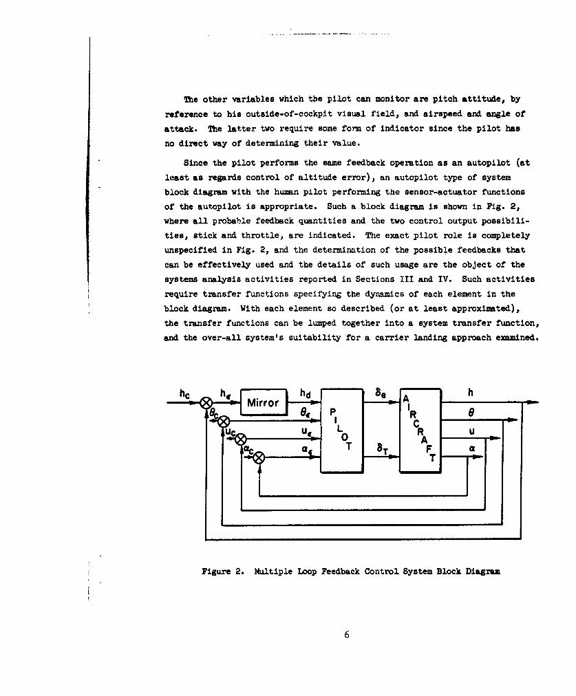
The other variables which the pilot can monitor are pitch attitude, by

reference to his outside-of-cockpit visual field, and airspeed and angle of

attack. The latter two require some form of indicator since the pilot has

no direct way of determining their value.

Since the pilot performs the same feedback operation as an autopilot (at

least as regards control of altitude error), an autopilot type of system

block diagram with the human pilot performing the sensor-actuator functions

of the autopilot is appropriate. Such a block diagram is shown in Fig. 2,

where all probable feedback quantities and the two control output possibili-

ties, stick and throttle, are indicated. The exact pilot role is completely

unspecified in Fig. 2, and the determination of the possible feedbacks that

can be effectively used and the details of such usage are the object of the

systems analysis activities reported in Sections III and IV. Such activities

require transfer functions specifying the dynamics of each element in the

block diagram. With each element so described (or at least approximated),

the transfer functions can be lumped together into a system transfer function,

and the over-all system's suitability for a carrier landing approach examined.

I C

Figure 2. Multiple Loop Feedback Control System Block Diagram

6

D. 2RAnU ,mJOfl Or W01 S ZIDW

1 - Te Aixrorft

Reference 1 U derives longituainal transfer functions from the equations

of motion. The process is standard in stability and control analysis and

will not be repeated here. Note only that the same assumptions are used

(small perturbations, linearized equations, etc.). Also, the effect

of a 40 glide angle on the transfer functions is negligible, so level

flight equations can be used.

Because most of the possible pilot roles involve simultaneous nanipu-

lation of stick and throttle, "coupling" transfer functions (Ref. 11)

appropriate to each multiple loop situation are also required. These arenot as common as the conventional transfer functions, so their detailed

derivations are given in Appendix A. The notation used therein is main-

tained throughout the rest of this report and is consistent with that of

Ref. 11.

Seven aircraft were used for specific case studies because their

minimum approach speed is reported (Ref. 1) to be dictated by the "ability

to control altitude or arrest rate of sink." These aircraft are the F8U-1,

FTU-3, F4D-i, FIIF-1, FgF-6, F-IOOA, and F-84F. The aerodynamic and

physical data on each are compiled in Ref. I and were used to compute

trim conditions and the corresponding nondimensional derivatives. These

derivatives were converted to dimensional form and used in the transfer

function computations. The trim speeds selected for investigation were

the average flight test minimum approach speed plus and minus about sevenknots. This spread was picked because the mean approach speed used in

fleet squadrons is usually about seven knots higher than the flight testreported minimum acceptable value, and the selected interval allows

examination of the effect of this nominal speed change.

7

2. US1Pilot

The form of the pilot describing function* is

YP MKp - T (TLs + 1)M- K~,e (TIs + I)(TNs+ ) (I)

where T - pilot reaction time

TN = pilot neuromuscular lag (his actuatorlag) time constant

Kp = pilot gain Pilot sets these

TL = pilot-adopted lead time constant as required by

TI - pilot-adopted lag time constant I the system

The nearomuscular lag time constant is of the order of 0.10 sec for center-

stick control and contributes only slightly in the pilot's effective band-width region (less than 1 cps). Accordingly, this lag is usually approximated

by e-0.1 8 and combined with the reaction time to give an "effective -t,"

typically about 0.20 sec in tracking situations. This eliminates the (TNs +1)term from the transfer function, so that the simplest form characterizing

the pilot is a gain plus a time delay,

SKe S (2)

In this simple form, the pilot's gain is Just the amount he moves the

control (T sec later) in response to a given magnitude of observed error.

The criteria which the pilot uses to set his gain have been deduced byexamining measured pilot describing functions from many single-loop control

* It is important to note that only the quasi-linear portion of the

pilot's output is described by this form and that it does not implylinearity in the point-by-point sense, but rather on the average. Thus,e.g., threshold in perception and consequent discrete manipulations ofcontrol are still representable by Eq 1.

8

experiments. These are criteria specifying the kind of closed-loop tracking

system performance that the pilot desires. Briefly stated, the requirements

are:(a) A stable system

(b) Good low frequency performance (This may be interpretedas the ability to control the low frequency but relativelyhigh power disturbances, such as those associated withatmospheric turbulence, which tend to make the trackingtask more difficult. To the servo analyst this criterionrequires a flat closed-loop frequency response with a gainof 1.0 over the disturbance input range.)

(c) Adequate closed-loop damping for oscillatory closed-loopsystems (This requirement is considered met by the pilotwhen the closed-loop damping ratio is 0.35 or greater.)

If the pilot cannot meet these criteria with a simple gain response, he

adopts a servo type of equalization, (TLS + 1)/(Tis + i). This can be lead,

lag, lag-lead, or lead-lag, within his dynamic capabilities. When he is forced

to do so to meet the system performance requirements, his opinion rating of the

aircraft deteriorates. The more extreme the equalization required, the worse

is the opinion rating. Generating lead, which requires sensing error rate

(as opposed to error position, or magnitude) causes the most degradation in

opinion. Generating lag requires integration, or time averaging, of the

errors. Lag time constants can apparently be as high as 10 sec with only

minor effects on opinion (Ref. 6), whereas lead time constants greater than

about 1 sec are apparently quite difficult (Ref. 5).

A basic assumption regarding the pilot's equalizing efforts is that he

always makes the minimum (or easiest) adjustments that he can get away with.

If extreme adjusting on his part only slightly improves the system, then he

will not make the effort. This carries over to multiple loop control situa-

tions in the assumption that he always closes the minimum number of loops

that gives satisfactory control. In other words, he will only control as

many variables as he has to in order to complete the approach.

To summarize qualitatively the mathematical description of the pilot's

servo characteristics, he prefers to operate as a simple gain controller, the

major limitation to this ability being his reaction-time-limited controllable

frequency range. If necessary for system stability or for good low frequency

control, he will adopt equalization using minimum adjustments, similar to

9

those that a good servo or autopilot designer would specify. However, a

system requiring large amounts of equalization will not get a good handling

qualities rating from the pilot.

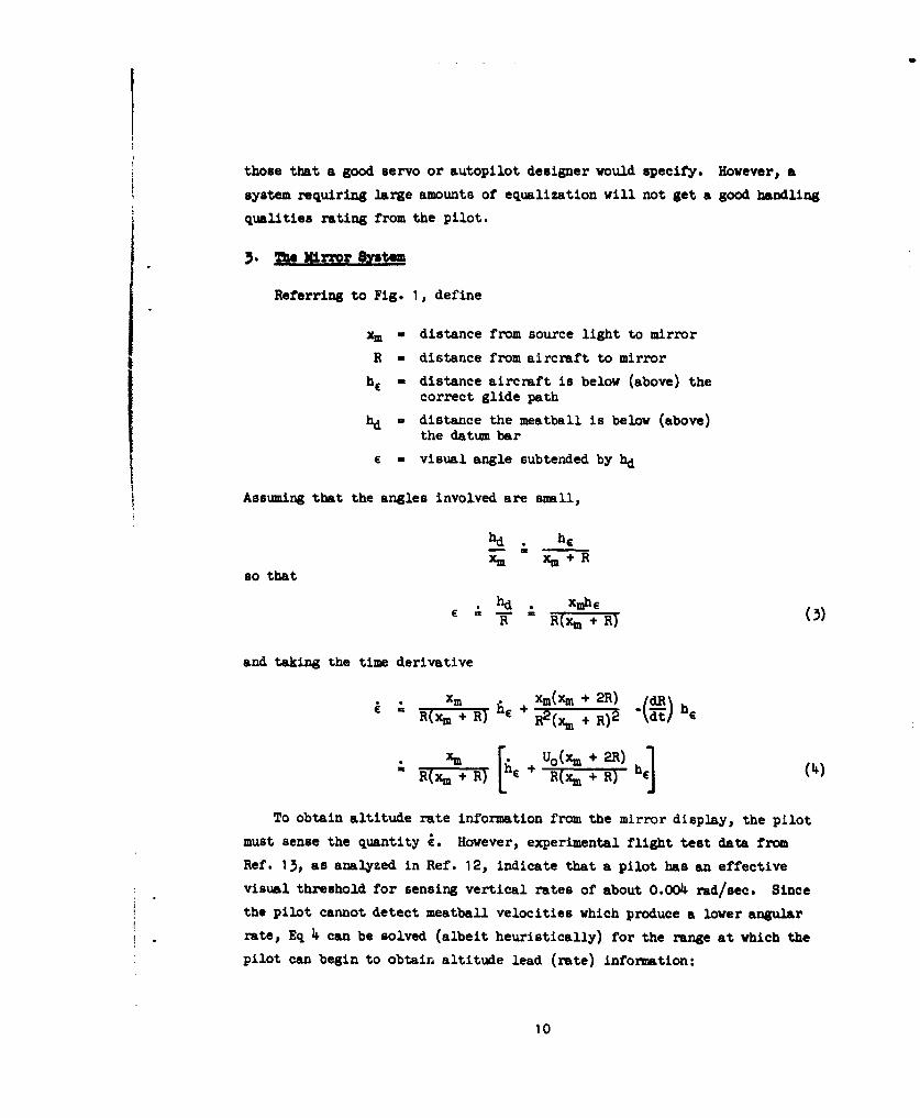
~.The Xtn'oi' System

Referring to Fig. 1, define

xm - distance from source light to mirror

R - distance from aircraft to mirror

he - distance aircraft is below (above) thecorrect glide path

hd - distance the meatball is below (above)the datum bar

e = visual angle subtended by bd

Assuming that the angles involved are small,

hd . he3; xm+aR

so that

e. xmhIER - R(xm + R) (3)

and taking the time derivative

xm Xm(Xm + 2R)"- R(xm+R) R" h.R)2 dti

_ _. Uo(xm + 2R)(

"-R(xm + R) [ + R(xm + R) h (4)

To obtain altitude rate information from the mirror display, the pilot

must sense the quantity i. However, experimental flight test data from

Ref. 13, as analyzed in Ref. 12, indicate that a pilot has an effective

visual threshold for sensing vertical rates of about 0.004 rad/sec. Since

the pilot cannot detect meatball velocities which produce a lower angular

rate, Eq 4 can be solved (albeit heuristically) for the range at which the

pilot can begin to obtain altitude lead (rate) information:

10

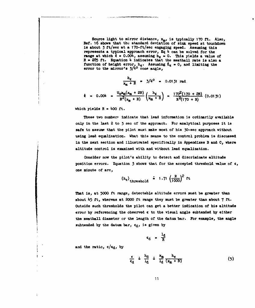
Source light to mirror distance, x, is typically 170 ft. Also,Ref. 16 shows that the standard deviation of sink speed at touchdownis about 3 ft/sec at a 170-ft/sec engaging speed. Assuming thisrepresents a typical approach error, Eq 4 can be solved for therange at which A = 0.004, assuming he - 0. This yields a value ofR - 285 ft. Equation 4 indicates that the meatball rate is also afunction of height error, h . Assuming fE - 0, and limiting theerror to the mirror's 3/4o cone angle,

h6e - /14° - o.4031 red

a . Uoxm(xm + ) ( 1 I 10+ 211 (0.0131)" R2(xm + R) m + " R 20 70 + R) 0o1)

which yields R - 400 ft.

These two numberF indicate that lead information is ordinarily available

only in the last 2 to 3 sec of the approach. For analytical purposes it is

safe to assume that the pilot must make most of his 30-sec approach without

using lead equalization. What this means to the control problem is discussed

in the next section and illustrated specifically in Appendixes B and C, where

altitude control is examined with and without lead equalization.

Consider now the pilot's ability to detect and discriminate altitude

position errors. Equation 3 shows that for the accepted threshold value of e,

one minute of arc,

(hE)threshold - 1 .71 (.)2 ft

That is, at 5000 ft range, detectable altitude errors must be greater than

about 45 ft, whereas at 2000 ft range they must be greater than about 7 ft.Outside such thresholds the pilot can get a better indication of his altitude

error by referencing the observed e to the visual angle subtended by either

the meatball diameter or the length of the datum bar. For example, the angle

subtended by the datum bar, ed, is given by

Ed=T

and the ratio, e/ed, by

E . hd. xm he7d d -q l(x,+R)1

In other words the gain, between the observed meatball height measured as a

fraction of the datum bar length, and the altitude error, is inversely pro-

portional to range rather than range squared as in Eq 3. Therefore, in the

analytical work described later it is assumed that the mirror display gives

only a gain change, and its dynamic and time-varying characteristics are

ignored, especially since they do not vary significantly with aircraft

approach speed.

In either case, the predominant effect of the mirror dynamics is to

introduce a time-varying (range-varying) gain in the altitude loop. This

time variation is not sensitive to small (10 percent) changes in approach

speed and can be eliminated as a speed-sensitive factor in setting the

minimum approach speed (however, it may be an important contributor to

the over-all difficulty of the approach task). The possibility of obtaining

altitude rate information from the mirror aid is practically nil and is not

a factor in setting any one aircraft's minimum speed (lack of such informa-

tion nay also be an important part of the carrier approach problem).

12

53'!ION III

Lm -Loop CIAMRISTIOBs or 108513 PILTnG T3CfIq1

The previous section described the mathematical characteristics of the

individual elements of the system shown in Fig. 2; this section will con-

sider the effects of the alternative ways of closing the loops shown in

that figure. There is a continuing debate among pilots as to how the

carrier approach should be flown. That is, should altitude be controlled

with stick and airspeed with throttle or should altitude be controlled withthrottle and airspeed with the stick? Current fleet squadron publications

recommend the latter method (h -> 5T, u -> Be), although they often say to

control airspeed with attitude (i.e., pitch attitude). MaMn test pilots,

on the other hand, recommend the first method (h -> be, u -4 -5T). The

subject of this debate, "what is the optimum control technique for carrier

approach?," may be paraphrased herein to "what are the optimum feedback

loops for the pilot to close?" This section will compare the characteris-tics of three potential methods for controlling the approach by comparing

their closed-loop frequency response characteristics.

There are four output variables that the pilot can use for control

purposes, as indicated in Fig. 2. These are altitude (relative to the

desired glide path), airspeed, angle of attack, and pitch attitude. Of

these, both altitude and pitch attitude are discernible to the pilot by

reference to the mirror display and horizon. In order to determine air-speed or angle of attack, however, the pilot must shift his focus to scan

some instrument within the cockpit area. In addition to the usual instru-

ment panel airspeed indicator, current Navy jet aircraft have an angle of

attack "indexer" mounted on the glare shield over the instrument panel.

This instrument gives the pilot an "on speed" signal for about 2-1/2 knots

either side of the desired approach speed, then indicates "slightly slow

(fast)" for the next 2-1/2 knots, and finally indicates slow (fast) for all

speeds beyond that range.

The reason airspeed and angle of attack can be referred to synonymously

during the approach is that altitude and pitch attitude loops are always

13

assumed closed by the pilot. If these loops are reasonably tight, then two

degrees of freedom are removed from the system and airspeed and angle of

attack are closely dependent. The angle of attack indexer is always heavily

damped (i.e., lagged) to filter out short-period oscillations, so the result-

ing low frequency variations give a direct indication of airspeed changes.

This assertion is borne out analytically in Appendix C.

Since there are four control variables (h, e, u, a) and two controls

(se, 5T), a large number of potential control techniques could be studied.

Practically, however, the list can be narrowed to three possibilities. These

three are discussed in the reminder of this section.

A. PILOT CLOMt3 OF M e -> be L4OP

It has been assumed in all of the analytical work discussed in following

subsections that the pilot always closes a pitch attitude loop, e -> 8e* In

other words, he uses the elevator to hold to his selected approach attitude.

There are several Justifications for this assumption:

1. It is the only loop useful in controlling short-periodmotions (remembering that the a indexer is highlydamped).

2. It is a powerful way to increase phugoid damping becauseit effectively provides altitude rate damping (forphugoid motiouAs, ,rhere a - constant, • = Uo7 ; U06).

3. There is ample evidence from time histories of carrierapproach that the pilot in fact does this (these showa high frequency elevator motion at what would be theclosed-loop short-period frequency).

4. The pilot gets benefits I and 2, regardless of how hechooses to control altitude or airspeed, merely bycontrolling his pitch attitude relative to the horizon.

To give a more quantitative example of the benefits of attitude control,a typical carrier-based Jet aircraft has a short-period frequency of about

1.5 rad/sec and a lightly damped phugoid (p -L 0.10) with a frequency of

about 0.20 rad/sec (see Appendix C). Closing the 6 -0 be loop with enough"1"gain" (a measure of the pilot's corrective control movements) to double

the short-period frequency will increase phugoid damping to Cp ? 0.80 and

14

decrease phugoid frequency slightly. The pilot now has an "equivalent

airframe" with double the initial static stability and at least an eight-

fold increase in phugoid damping, just from closing the 9 -> 5 e loop.

With this basic "inner loop" assumed closed, and the resulting well-

damped "equivalent airframe," it is instructive to compare the effects of

various possible methods of altitude control. This is assumed to be theprimary task in a carrier approach, with airspeed control secondary. The

following subsections discuss altitude control with elevator, with throttle,

and with combined elevator and throttle. The discussions are pr-imarily in

terms of the closed-loop frequency response characteristics that the pilot

obtains, using the specified control technique. An effort has been made to

keep the presentation as nonmathematical as possible, however, so the

arguments presented below attempt also to appeal to physical reasoning.

Should these arguments not be convincing, recourse may be had to the appen-

dixes for more detailed and technical expositions.

B. AMT= CO WMT ELVATOR (h -- be, e - be, u or . -* OT)

Changes in altitude and airspeed are phugoid phenomena; in other words,

they are associated with the low frequency phugoid mode. Closure of one or

more control loops does not change this basic situation, but it may change

the phugoid frequency and damping significantly. Therefore the effect of a

loop closure on altitude control may be described primarily by its influence

on the phugoid mode. The types of loop closures to be considered are

associated with (1) a simple gain (with reaction time) pilot transfer func-

tion (i.e., proportional control), (2) pilot lead adaptation (i.e., propor-tional plus rate control), and (3) the effect of flight at speeds above and

below minimum drag. As was shown in Section II, the pilot must operatethrough most of the approach as a pure gain in altitude control. Root locus

plots in Appendix B show that this loop closure (h -I be) will increase the

phugoid frequency and, initially at least, will cause almost no change in

damping (total damping, tw, as opposed to damping ratio, t). As gain is

further increased the frequency will continue to increase but damping will

begin to deteriorate until the phugoid oscillation finally becomes unstable.

Starting from the well-damped condition resulting from the 6 -0 be inner

15

loop, the phugoid frequency can typically be increased by a factor of four,

e.g., from 0.20 rad/sec to 0.80 rad/sec, before instability results and can

almost be doubled at constant damping. This very desirable "stiffening" of

the altitude control mode occurs regardless of speed relative to that for

minimum drag. The only drawback in the phugoid frequency K is the

decrease in damping when the pilot's gain gets too high.

This drawback can be overcome by the addition of altitude rate damping.

But, as shown in Section II, pilot-generated lead (i.e., rate damping) comesfrom his sensing "meatball" vertical velocities and is available only in the

last few seconds of the approach. Assuming that a 1-sec lead time constant

is the best the pilot can do (see Section II), then the benefit to phugoid

damping will only be a slight improvement over the no-lead case, as illus-

trated in Appendix B (Fig. B-11). Larger lead time constants can greatly

improve height control with elevator, but are well beyond human pilot capa-

bility using the existing optical landing system for height control. Since

the assumed pilot maximum lead of about 1-sec does not give a significant

improvement in height control, it is concluded that the system's phugoid

characteristics with a straight gain assumed for the pilot transfer function

will best represent the altitude-control-with-elevator case. To repeat,

these phugoid characteristics are (1) a "stiffening" of frequency for low

pilot gains, but (2) a decrease in damping leading to system instability as

pilot gain is increased too much.

The final consideration, and a most important one, is the effect of

reducing the approach speed below minimum drag. When an h -4 5e loop is

closed, a very low frequency time constant is introduced into the system

which is associated primarily with the airspeed response of the system. As

the aircraft goes from the front to the back side of the drag curve, this

time constant shifts from being stable to being unstable. Thus, when

trimmed on the back side of the drag curve,* the increased drag, as the

*Comments pertaining to the back or front side of the drag curve, or tospeeds below or above that for minimum drag, hereafter imply operation withrespect to the speed at which the time constant changes sign. As shown inRef. 2, this speed, while primarily a function of drag characteristics, isalso influenced by thrust variations with speed (for constant throttle setting)and by thrust eccentricities about the c.g. which make the partial derivativeof pitching moment with respect to speed, CM., nonzero.

16

aircraft slows down in response to up-elevator motions intended to increase

altitude, will. actually cause altitude to decrease (after the initial

transients die out). Further up-elevator deflections to increase the now

steadily decreasing altitude will result in a divergent altitude motion

(increasing rate of descent) characterized by the negative time constant

alluded to above. Hence comes the pilot's complaint of "ability to control

altitude or arrest rate of sink."

The pilot can stabilize this divergent mode by overpowering drag changes

with thrust changes. Closure of either an airspeed (u --> ST) or angle of

attack (a --> 6T) loop with the throttle will perform this function and, in

essence, convert the back side condition to an effective front side condi-

tion. But the pilot is then required to close a third loop and to use more

than some minimum gain in that loop in order to stabilize the system.

Requiring such throttle activity on the pilot's part in order to achieve

system stability (the highest priority closed-loop system performance

criterion postulated in Section II) dictates that he have a "good" display

of airspeed or angle of attack error information in order to proportion his

throttle corrections. A "good" indicator should (intuitively) be located

so the pilot does not have to shift his focus from the meatball, and it

should provide a linear and smoothly responding error signal. The cockpit

airspeed indicator is essentially inaccessible to the pilot because it

requires shifting his gaze completely away from the mirror. The m indexer,

mounted on the top of the instrument panel's glare shield, is almost within

the pilot's view, but it suffers from the nonlinear nature of its indication

(which gives essentially only five speed indications-on speed, slightly

slow or fast, and too slow or fast). Since the m indexer does not satisfy

the criteria for a "good" display, the pilot's task is made more difficult

than necessary for closing this control loop. In support of this assertion

it should be noted that when an automatic throttle is installed in an air-

craft to perform this function for the pilot, he is willing to reduce his

minimum approach speed (see, e.g., Ref. 14).

To summarize the characteristics of altitude control with elevator, the

basic phugoid oscillation is stiffened by pilot pure gain, or proportional,

control. Damping deteriorates as gain gets high, and the lead equalization

17

that the system needs is beyond human pilot capability with the present mirror

display. These phugoid characteristics occur on both front and back side of

the drag curve, but on the back side a drag instability exists that requires

pilot closure of an auxiliary throttle loop. Closure of this loop is predi-

cated on a usable display of airspeed or angle of ettack error information.

0. ATI!T O 1OL W=l TM0TLR (h --* 8T, e -3 be, u or b-*e)

Control of altitude with throttle has distinctly different characteristics

than control with elevator. In the first place, this method of control does

not have the basic instability on the back side of the drag curve that is

inherent with the h --* be loop closure. The reason for this is that pilot

operation of the throttle to hold altitude eliminates the thrust deficiencies

that occur with elevator control. So the basic difference in response

dynamics between front and back side of the drag curve operation is no longer

present.

A second important difference is in the closed-loop phugoid characteristics.

Pilot gain in an h -w 5 T loop has the effect of decreasing (total) damping of

the phugoid while altering frequency only slightly (decreases for low gain,

then increases). The low frequency and damping results in large phugoid

oscillations and sluggish response. The aircraft becomes more susceptible to

the high power but low frequency atmospheric turbulence disturbances which

make control difficult.

A final point is that a much larger amount of lead equalization (rate

damping), using throttle as the control, is required to make the phugoid

characteristics "good" in the sense that elevator control in conjunction with

a reasonable lead time constant is good (high frequency and high damping).

The cause of these poor closed-loop dynamics is the long time lag between

thrust changes and lift changes, too long to be overcome by a reasonable

lead. Navy jet aircraft have a low thrust-line angle of attack in the

approach configuration, 5 to 20 being typical. Since the pilot is trying

to control altitude, or height, he should be using a vertical force.

Instead, he is applying a nearly horizontal force and then converting the

resulting airspeed change into lift by holding e, and possibly u or m,

18

constant with the elevator. Thin control method has such a long lag between

thrust change and height change that even very ltrge 1,rid time constants ran-

not overcome the lift lag and produce a well-damped high frequency system.

In conclusion, then, this method of control is characterized by a

deterioration in phugoid response a8 pilot throttle gain increases. Its

only virtue Is ite basic stability on the back side of the drag curve.

D. Am== Co0 OL WITH IzmVATOR AnD !I (h -I le, IT; e -. Be;)u or M -4 e, BT

The final possibility open to the pilot is to use both stick and throttle

to correct the observed errors in altitude (and airspeed or angle of attack).

The net effect of this control technique will be to combine the features of

the two previous methods, the degree of combination depending on the relative

vigor with which stick and throttle are used. In other words, the two

preceding methods represent the limiting cases for this more general method.

Considering operation on the back side of the drag curve, the effect of

the throttle will be to stabilize the altitude divergence caused by the

elevator loop closure. There will be a minimum ratio of throttle to elevator

motion required to achieve system stability (elimirate the thrust deficiences),

and this minimum value will increase as the (back side) slope of the drag

curve increases. On the other hand, as the throttle movements become larger

relative to elevator control, the undesirable effect of degrading the phugoid

frequency and damping will increase. Obviously there must be some compromise

made by the pilot between stabilizing the altitude-divergence mode and

destabilizing the phugoid mode. This compromise requires that he very

carefully ratio (or coordinate) his stick and throttle movements.

The main advantage of this control technique, then, is the potential

combination of the beneficial characteristics of the two other methods,

system stability and good phugoid response, without relying on closing an

auxiliary u or m loop. The main drawback is the very precise coordination

of stick and throttle required of the pilot in order that the optimum balance

between these two characteristics be maintained.

19

3. PZLOE OPNON OOMnflRATION8

Table I, which summarizes the foregoing, shows that the pilot is facedwith three choices as regards his basic control of altitude; he can use

elevator alone, he can use throttle alone, or he can use a combination of both.

TABLE ISMOMRY OF PREDOMINANT LOOP-CLOSURE EFFECTS

EFFECT ONLOOP Alit dPhugoid Short Period Altitude

Control

9 -0' be Increases damping consid- Decreases damp- No effecterably, decreases frequency ing slightly,slightly increases fre-

quency

h -b 5e Decreases damping, increases No major effect Destabilizesfrequency markedly

h -6 5T Decreases damping slightly, No major effect Stabilizesdecreases then increasesfrequency

h - be, 5T Combines above

The advantage of elevator alone is the high closed-loop phugoid frequency

attainable, which implies a good, fast-responding, altitude tracking systemable to suppress atmospheric turbulence inputs and follow carrier motions.However, this system has the disadvantage of requiring a minimum level ofauxiliary throttle activity to avoid instability when flying on the back sideof the drag curve. The second method is to control altitude with throttle.

This sytem is characterized by a low frequency, poorly damped phugoid whichimplies a sluggish, oscillatory response; but the system is inherently stable.The third system, coordinated stick and throttle control, combines the goodfeatures of the other two-high phugold frequencies with system stabilityprovided by the h -* 8 T closure, The drawback is that the pilot must ratiohis stick and throttle movements carefully to achieve this good control.

20

Which method will the pilot use? The argument for his using the first

method (h -i be) is that it gives a fast-responding altitude control. It

does, however, require that angle of attack or airspeed information be

presented to the pilot in such a way that he can use it. The argument for

his using the second method (h -> bT) is that it is initially stable so

there is no minimum requirement for system stability. The penalty is that

this method has the poorest control characteristics. And finally, coordi-

nating stick and throttle to control altitude (h -> be, BT) can have the

good features of both, but requires a very precise coordination between

the two controls.

The answer to what the pilot can or will do depends to a large extent onthe pilot's dynamic capabilities in multiple loop tasks (his ability to per-

form the required sensor-actuator functions utilizing the available informa-

tion) as well as on the previously described closed-loop system performance

characteristics. In the article quoted below (Ref. 15), a Navy test pilotdescribes the pilot's viewpoint of the system characteristics Just discussed.

"The pilot instinctively attempts to make glide path correctionsinitially with longitudinal control only. It is therefore extremelydesirable that the airplane have maneuvering capability at a constantthrust setting for small changes in angle of attack (approximately1-2 degrees). If, as in the F8U, these small changes in angle ofattack produce correspondingly large excursions in airspeed, thealternative technique must be evaluated, that of varying rate ofdescent with power. In this type of approach, the airplane is main-tained at a desired angle of attack and thrust corrections are usedexclusively to make glide path corrections. . . When the desiredvertical accelerations cannot be obtained with this technique, as inthe case with the F8U, a combination of two techniques is requiredin which both thrust and longitudinal control are initiated simulta-neously. This technique produces the necessary rapid corrections inglide path although it requires precise coordination throughout thecontrol process."

The pilot is saying, then, that his priority ranking of the systems is thesame as the order in which they were discussed, except that he seems to rule

out elevator-alone control of altitude below minimum drag speed. From thesystems analysis point of view this is clearly the wrong thing for him to do,yet the next section presents an analytical development which gives convinc-ing evidence that the pilot in fact does choose the throttle-control-of-

altitude method. The last section presents some possible arguments as to

why this should be so.

21

SECTION IV

A UMNIX APPROACH SPE CRITIONDERVD I= OOMD KUL(M T LOOP CUID•AIMONS

A. DERIVATION OF MIE CRI tION

The previous section has shown the advantages and disadvantages of the

various control techniques that are available to the pilot for making the

approach. In this section one particular control method will be used as

the basis for deriving a criterion for predicting the minimum acceptable

approach speed.* For the analysis, it is assured that the pilot uses the

elevator to control pitch attitude and the throttle to control altitude.

The analytical expression for the closed-loop phugoid frequency, in terms

of aircraft stability parameters and pilot gain terms, is derived from asimplified set of equations. Then it is shown that at a certain speed below

minimum drag this closed-loop frequency begins to decrease as pilot gain in

the elevator loop increases. Reasons are explained why this should representthe minimum acceptable approach speed in terms of altitude control.

A review of the conclusions drawn in Section III indicates that altitude

control problems in the approach are low frequency in nature; that is, they

are associated with the (closed-loop) phugoid motions of the aircraft. This

qualitative assertion is borne out quantitatively in Appendix B, where it is

shown that the phugoid branch of the altitude control root locus is the onepresenting control problems. This occurs regardless of the control technique

chosen by the pilot, but most pronouncedly so when the pilot attempts to

control flight path with throttle. Since short-period attitude control isgenerally not a problem, it is safe to neglect the short-period terms in the

equations of motion and look only at the phugoid equations. This has the

advantage of reducing the order of the equations to the point where theyprovide easily factored solutions. Since the phugoid frequencies are of the

order of 0.2 rad/sec, pilot reaction time, T, will contribute only slightly

*Reference 9 contains a preliminary exposure of these results.

22

in this region and need not be included in the pilot model. Also, since lag

equalization is generally not helpful here (Appendix B) and lead time con-

stants, TL, corresponding to the pilot's desired maximum of about 1 sec have

no benefit, the influences of pilot equalization in the frequency region of

interest will also be negligibly small. Both T and TL effects will contribute

phase angle changes of only a few degrees at these low frequencies and there-

fore cannot affect the results. Thus the pilot transfer functions can be

approximated as pure gains (simple proportional control):

Y Me

(6)I y " - a Kph

The phugoid equations of motion (Ref. 2), assuming X~e - 0, are

(s-Xu)u -X~w +ge +0 a - TI

-Zu +(s - Z)w -Uose +0 M Z *Z• 6 e (7)-KMu -Mw +0 +0 - %bT + ebe

0 w -Uoe +sh U 0

where the last equation expresses the kinematic relationship between altitude,

h, and the independent degrees of freedom, u, w, e. Recognizing that Eq 6

may be rewritten as

be = KpeeC a -Kpee (8)

5T - Kphhh - "Kphh (9)

(because the "error signal" to the pilot is the reverse of the aircraft's

motion), substitution of Eq 8 and 9 into the right side of Eq 7 eliminates

23

the control deflection variables and yields a new set of equations with"equivalent stability derivatives." This set of equations gives a new charac-

teristic determinant, which is the system's closed-loop characteristic equation.

It can be expressed in the form

asd + be2 + cs + d a 0 (10)

where the coefficients a through d contain aircraft stability derivatives and

pilot gain terms, This closed-loop equation can then be factored into the

form

K(s + T;)(s2 + 2 tia ýs + O2) 0 (i

(the double prime notation indicates two loops have been closed), and the

closed-loop system tested to see if it meets the pilot's system requirements

(performance criteria). This procedure is the one followed in Ref. 9 and

completely avoids the use of servoanalytic methods. However, a more instruc-

tive procedure, to follow, uses the conventional servoanalysis method of

successive loop closures, rather than the "augmented derivative" approach,

to arrive at the same result. More insight into the effect of each closure

can be gained by this latter method, as will be demonstrated. Transfer

function equations for the multiple feedback loops involved are derived in

Appendix A for three degrees of freedom, and since the basic process is the

same, no Justification of the specialized phugoid transfer function form

used here will be presented.

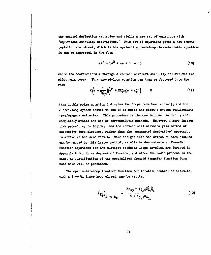
The open outer-loop transfer function for throttle control of altitude,

with a 0 --1 8 e inner loop closed, may be written

NhbT + (N12

e -0 be A + Y beeNbe

24

where the various terms of interest in this case are:

Nh~- (~j~ -~i~~,' 8 + the h -> BT~ transfer functionSThT/ numerator (phugoid only)

.h~ ~ ~ 8 ae)( + y I ), th -l 6T --> 5. coupling

A -Mae(.2 + 2tpck~s + aq, the open-loop characteristic(a (phugoid only)

Nee M ies ( + -L)(s + the 8-> 8 transfer function(91 O( T02) numerator Tphugoid only)

Ybeo - KP9 ; YbTh - Kph see Eq o

The closed-loop will be determined in two steps, by first closing the

6e -> e loop and then the h -> 6T loop. Adding the two denominator terms

in Eq 12 gives the new characteristic equation with the 0 -> be inner loop

closed:

M (I ' - (e E) (s2 + 2t

{ . + K)s2 + (2ppu: + Ke9 L + s + + Ke T9 1 Te )

where the single prime notation denotes one loop has been closed. Equating

coefficients identifies

MbeKe * -Kpe • ( 4)

2 tpCa, + K9 +

_i1 + K

2 + TeT•e 2 (16)

1 +2e

25

In finding the 0 -) be loop effect on the altitude control numerator, it

is now assumed for simplicity that the thrust line passes through the c.g.

of the aircraft. For this special case, MIT - Mu - 0, and the two time

constants associated with the numerator of Eq 12 can be shown to be identical,i.e.,

h Tj. X + k (1 7 )

The altitude control zero, I/T, thus is not a function of Ke and is in fact

also given by Eq 17.

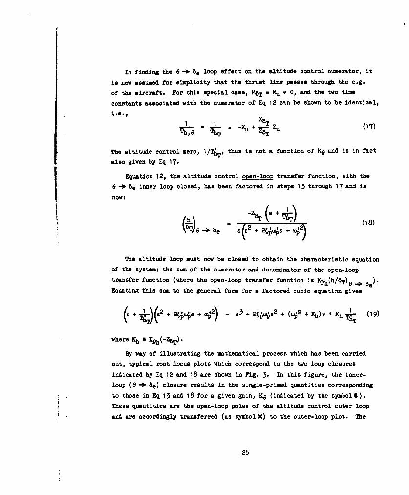
Equation 12, the altitude control open-loop transfer function, with the

n -: be inner loop closed, has been factored in steps 13 through 17 and isnow:

The altitude loop must now be closed to obtain the characteristic equation

of the system: the sum of the numerator and denominator of the open-loop

transfer function (where the open-loop transfer function is Kph(h/ST) 0 ->e.

Equating this sum to the general form for a factored cubic equation gives

\+ j(2 + 2t;4s + ,2 s3 + 2j4•s2 + (S2 + Kh)s + Kh - (19)

pa TO TAT

where Kh s Kph(-Z7.).

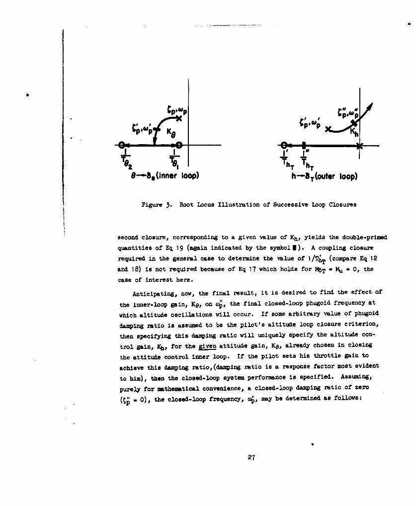
By way of illustrating the mathematical process which has been carried

out, typical root locus plots which correspond to the two loop closures

indicated by Eq 12 and 18 are shown in Fig. 3. In this figure, the inner-

loop (9--0 be) closure results in the single-primed quantities corresponding

to those in Eq 13 and 18 for a given gain, K6 (indicated by the symboll).

These quantities are the open-loop poles of the altitude control outer loop

and are accordingly transferred (as symbol X) to the outer-loop plot. The

26

I kTTo. +hT ThT

8---Uinner loop) h--aT(outer loop)

Figure 3. Root Locus Illustration of Successive Loop Closures

second closure, corresponding to a given value of Kh, yields the double-primed

quantities of Eq 19 (again indicated by the symbol 1). A coupling closure

required in the general case to determine the value of 1/T (compare Eq 12

and 18) is not required because of Eq 17 which holds for MBT - Mu - 0, the

case of interest here.

Anticipating, now, the final result, it is desired to find the effect of

the inner-loop gain, Ke, on ", the final closed-loop phugoid frequency at

which altitude oscillations will occur. If some arbitrary value of phugoid

damping ratio is assumed to be the pilot's altitude loop closure criterion,

then specifying this damping ratio will uniquely specify the altitude con-

trol gain, Kb, for the given attitude gain, K6 , already chosen in closing

the attitude control inner loop. If the pilot sets his throttle gain to

achieve this damping ratio,(damping ratio is a response factor most evident

to him), then the closed-loop system performance is specified. Assuming,

purely for mathematical convenience, a closed-loop damping ratio of zero

(1 - 0), the closed-loop frequency, 4, may be determined as follows:

p0

27

Expanding the left side and then equating coefficients in Eq 19,

2 terms: - + +

aterms: 4TT- 240' + 2 (20)

Constant terms: 1 -2 = 1h

Setting j - 0 in the above equations and eliminating Kh and Tj" yields

1 ,ý2

( , ,2 T A T ( 2 1 )

P o 4

Noting that 1/T4T is independent of Ke for this special case, the single-

primed quantities are defined in Eq 15, 16, and 17, and Eq 21 can be written

in the more basic form

1 + K 6 e 1 e(4)2 ---- \ T e1 o2 ) (22)( p) - +00 1 2ýp a. - e + T19

Equation 22 indicates that for t" a 0 (and the general trends of Fig. 3

indicate that the results are not appreciably altered by small, finite values

of •") the closed-loop phugoid frequency is a function only of the pilot'sp

6-loop gain and of basic aircraft stability parameters. In order to find the

effect of that 6-loop gain on the phugoid frequency, the partial derivative

is taken, giving

W 0 T9.O oh T,922 Te h(Tp I 2Mcl)+(~~ L (23)a+ K) -" 1+P 1 - Ke ( + 1)2

28

The form of Eq 23 indicates the possibility of a change in sign for some

combination of the numerator parameters, which are all functions of airspeed.

It can (and will) be shown that this partial derivative is always positive

for flight on the front side of the drag curve but that at an airspeed some-

where on the back side of the drag curve it becomes zero, and, as speed is

further decreased, it becomes increasingly negative.

What is the significance of this sign reversal in terms of flying

qualities? The answer to this question may be determined by considering,

in frequency response terms, what the pilot wants for a closed-loop control

system. Since the phugoid frequencies are low, implying "sluggish response"

to altitude control efforts, the pilot's primary desire is to "tighten up"

this system by increasing the frequency (or, in servo parlance, the bandwidth)

of response. Furthermore, if he is making the approach through turbulent

air, it may be imperative that he increase the frequency in order to overcome

the gust spectrum inputs disturbing his aircraft. His normal reaction will

be to increase the gain in the attitude control loop; in other words, to

tighten up his elevator control. This increases inner-loop phugoid damping,

and, for flight on the front side of the drag curve, it also increases

But at some speed on the back side of the drag curve, tighter elevator con-

trol suddenly begins to degrade the aircraft's altitude response by decreasing

its bandwidth characteristic. The pilot senses that his normal elevator

control reactions are making altitude errors larger, yet he cannot remedy

the situation because increasing throttle gain only decreases the phugoid

damping. Decreasing his elevator gain allows larger pitch attitude oscilla-

tions although helping altitude control. Presumably this "control reversal"

effect, if it may be so termed, will be disconcerting enough to make the pilot

limit his approach to speeds at or above the reversal point.

A possible criterion for the minimum acceptable approach speed, based on

the previous argument, is therefore the reversal point given by setting the

partial derivative of Eq 23 to zero,

T9 I Te 2 2T)2

Eq 24 being valid for cases where the thrust line of the aircraft passes

through the c.g.

29

A review of all the assumptions made In the foregoing derivation may

be useful in clarifying the development. These were as follows:

1. Phugoid equations adequately represent the frequencyregion of interest

2. The pilot controls pitch attitude with elevator andaltitude with throttle, and may be approximated bya simple gain in each loop

3. The final closed-loop phugoid damping ratio is zero

4. The thrust line offset from the aircraft c.g. is zero

Assumptions 1 and 2 are not restrictive; that is, they are basic to the

handling qualities theory. Assumption 3 was made to predetermine the magni-

tude of the pilot's altitude control gain; and the specific value of t = 0

was chosen merely to simplify the form of the criterion. In Justification

of Assumption 3, it should be noted that for second-order systems in

single-loop tasks, at least, the pilot seems to set his gains to get a con-

stant damping ratio (or phase margin). The altitude control root locus in

Fig. 3 indicates that phugoid frequency increases as the damping ratio

decreases in the region near neutral stability. Therefore the pilot can

trade off ý and U or vice versa, in order to minimize his altitude errors.

It is difficult to predict what specific value of damping he would probably

choose, but any constant value will serve to show the trend of 4 as K9

changes.

The final assumption was made so that I/T1 would equal 1/Th. When

there is a finite thrust offset, 1/T1 becomes a function of the attitude

gain, K9, and the criterion in the form of Eq 24 is not valid. Then, to find

the speed at which the derivative is zero, it is simplest to revert to the

basic formula for 12 given in Eq 21, use two representative values of K6 to

compute values of 1/TAT, 2t , and finally aý 2 ; and take the derivative

asthe ratio, 2 /LKO. Values of K6 of 1 .0 and 2.0 are typical for pilot

attitude control and have been used in specific cases to compute this deriva-

tive; furthermore, the point of zero slope has been found to be more sensitive

to airspeed than to different (but reasonable) values of Ke. Thus the original

assumption that the thrust line offset is zero can be bypassed when necessary

and does not restrict the general applicability of the suggested criterion.

30

D. 2MXG ILI CREMlON: AOWLU BMZWD 110 IOUAND F0M TM NEC= APPmOAOI nP8In

Seven of the 21 aircraft for which aerodynamic data are tabulated in

Ref. 1 are specifically limited in carrier approach speed by "the ability to

control altitude or arrest rate of sink." For all seven, the minimum speed

was on the back side of the thrust-required curve. These seven are the

FMU-1, F7U-3, F4D-1, F-100A, F-84F, F11F-1, and F9F-6. Transfer functions

were computed for each aircraft for at least three flight conditions corre-

sponding to the flight-test-determined minimum approach speed plus and minus

about seven knots.* The partial derivative ( 11j2 I~e a vlae o

each aircraft at each speed using the general procedure outlined above.

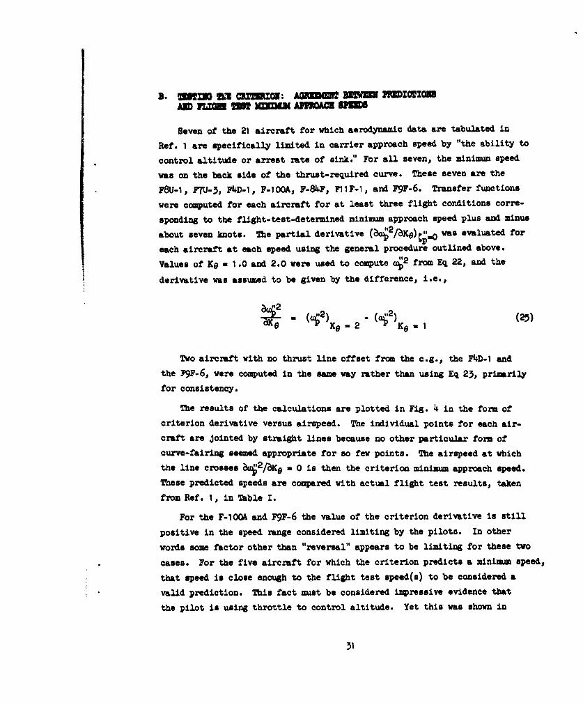
Values of K9 - 1.0 and 2.0 vere used to compute O 2 from Eq 22, and the

derivative was assumed to be given by the difference, i.e.,

& . "2) (02) (2)K9 - 2 K9 = I

To aircraft with no thrust line offset from the c.g., the F4D-1 and

the FgF-6, were computed in the same way rather than using Eq 23, primarily

for consistency.

The results of the calculations are plotted in Fig. 4 in the form of

criterion derivative versus airspeed. The individual points for each air-

craft are Jointed by straight lines because no other particular form of

curve-fairing seemed appropriate for so few points. The airspeed at which

the line crosses &wj2 /aKe . 0 is then the criterion minimum approach speed.

These predicted speeds are compared with actual flight test results, taken

from Ref. 1, in Table I.

For the F-100A and F9F-6 the value of the criterion derivative is still

positive in the speed range considered limiting by the pilots. In other

words some factor other than "reversal" appears to be limiting for these two

cases. For the five aircraft for which the criterion predicts a minimum speed,

that speed is close enough to the flight test speed(s) to be considered a

valid prediction. This fact must be considered impressive evidence that

the pilot is using throttle to control altitude. Yet this was shown in

31

TABLE II

COMPARISON OF CRITERION-PREDICTEDMINIMUM APPROACH SPEED AND FLIGHT TEST SPEED(S)

FLIGUT TEST SPEED CRITERION SPEEDAICR fT (Knots) (Knots)

FSU-1 133, 134, 13•5 132

FTU-3 108,* 115, 117 109

F4D-1 114,* 117, 119, 120 121

F-84F 132* I11

F11F-1 128, 131 125

F-IOOA 15•* None predicted for U0 > 140

F9F-6 115, 118 None predicted for Uo > 108

*FCLP (field carrier landing practice) result

Section III to be the poorest method (in terms of servo performance) of

altitude control. This raises the fundamental question of why the pilot

has chosen the nonoptimum system; possible explanations for his choice are

postulated in the following section.

One further item requires comment. When the F4D-1 values of 42 were

first computed, the reversal derivative came out negative at all speeds

around the flight test Vmin; in other words, the F4D-1 was below its

theoretical minimum. While rechecking the aerodynamic data it was noted

that the F4D-1 has a large elevator drag term, XBe being on the order of

0.30 Zke. This factor had been neglected in the machine program computing

the e -3 6e transfer functions since it is normally small, and when it was

included in those computations the criterion was successful in predicting

the approach speed. This fact has important design implications because

it indicates that a large positive significantly reduced the F4D-1

approach speed (or at least the criterion-predicted approach speed).

LLL

=~ I r-0 mI

0O

La.. 0i Ii0 ca. P. L.0 0Wd~-'

IadIe

(adme

33.

8STZON V

BUTWARY AND OOCLUSION

Multiple-loop analyses have disclosed that required piloting techniques

differ considerably between approaches made on the "back" and on the "front"

side of the drag curve. In the latter instance, the pilot can theoretically

make flight path corrections with the elevator alone, and does not need

throttle inputs except for "initial" trim power adjustments. Reference 15

points out that this is the natural way to fly the approach. However, when

the speed is decreased below minimum drag speed, the closed-loop system

becomes unstable if the pilot uses the stick as his altitude controller.

Several courses of action are then possible, depending on the type and

quality of information available to the pilot. Assuming only that available

by reference to the mirror-approach display (altitude-error and attitude),he can theoretically stabilize and control the system, for speeds less than

minimum drag, by controlling attitude with elevator and altitude with

throttle. The resulting closed-loop performance would appear marginal in

terms of bandwidth, especially for rough air and/or sea-state conditions.

But as speed is progressively reduced, the achievement of even this marginal

performance eventually becomes "negatively dependent" on elevator control.

Thus, while increasing "tightness" of attitude control with elevator improves

performance at speeds well above the approach speed, a similar increase in

attitude control "tightness" eventually begins to degrade performance as

speed is reduced. Such degradation is sure to be considered undesirable

because it means that the pilot, by trying hatder to control the system, is

actually making it worse.

Calculated minimum approach speeds based on incipient degradation (i.e.,

zero effect of "tightening" elevator control), match well with flight test

minimum speeds for five of seven aircraft suspected to be speed-limited

specifically by the "ability to control altitude." Although such corroborating

evidence is not completely conclusive, it lends considerable support to the

argument that, for aircraft operating on the back side of the drag curve,

1. Pilots choose to control altitude with throttle (inaddition to controlling attitude with elevator).Other methods with theoretically superior dynamicperformance are bypassed.

2. The "control reversal" effect, associated with thispilot-selected method of control is sufficientlydisconcerting to limit the minimum approach speed.The speed for incipient reversal therefore providesan easily calculated criterion for minimum approachspeed.

But what of the other control methods that are available to the pilot?

Assuming the additional information provided by suitable angle of attack or

airspeed displays, the pilot can theoretically use the elevator for height

and attitude control, and throttle to hold angle of attack or airspeed con-

stant. Essentially, the throttle zanipulations involved in this mode of

operation reverse the "backside" effect of an increase in drag as speed

decreases to an "effective frontside" net decrease in drag as speed decreases.

Thus the pilot gets good longitudinal response as long as he is able to

maintain thrust required with the throttle.

Another alternative is to coordinate stick and throttle to control altitude.

This theoretically eliminates the need for a good airspeed or angle of attackindicator and also permits the pilot to fly the approach using only two feed-

back loops. The benefits of fast-responding elevator control and stablethrottle control are obtained at the expense of a requirement for very care-

fully coordinated stick and throttle action.

In the course of arriving at these conclusions, other more complicated

(up to five feedbacks) modes of control have also been investigated analyti-cally. Although some of these were found to result in suitable systems, they

are, in the final analysis, considered inappropriate because the gains in

performance (if any) are not commensurate with the increase pilot effort

required.

Both of the alternative piloting techniques discussed above are theoreti-

cally superior to the throttle-alone method of controlling altitude in the

approach. They both should eliminate the "ability to control altitude or

'5

arrest rate of sink" as a dynamic control problem in carrier approach. The

question then arises as to why this type of limitation apparently exists,

since m information is displayed in all current carrier aircraft. Also, why

is a criterion based on only altitude and pitch attitude information so

successful in predicting the speed at which this limitation occurs? If it

is assumed that the criterion's success indicates that the pilot does in

fact use throttle to control altitude, it must then be explained why he has

chosen the nonoptimum system. The following are possible explanations:

1. The nonlinear type of . indexer installed in fleet air-craft prevents effective pilot use of this device, thusrequiring that the pilot revert to the other (h -> bT)technique.

2. It is beyond the pilot's dynamic capabilities to effec-tively close three loops and use the m indexer inmultiple-loop tasks.

3. The closed-loop performance benefits which the pilot isdynamically capable of achieving by the best method arenot required due to the low frequency content of theforcing func-tion (carrier wake, atmospheric turbulence,carrier motions).

4. The pilot is unaware of the benefits to be gained byclose control of a with throttle, and is performing thesimpler task (two loops versus three) which still yieldsacceptable results.

These explanations have one common factor: they depend on assumptions as

tD the pilot's actual performance in the loop. The analyses used as the

basis for this report's conclusions are all predicated on extrapolating

actual human transfer function measurements in single-loop tracking tasks to

predicted behavior in multiple-loop flight control situations. To investi-gate these predictions and to answer other questions which may arise, it is

necessary to perform a series of well-designed flight simulator experiments.Results of such experiments which are inconsistent with the present mathe-

matical pilot model will give rise to refinements in the analysis processwhich may in turn lead to auxiliary experiments. This type of experimental

program, and the attendant analysis-refinement activities, is a logical

extension of the purely analytical work reported herein. It is worth noting

36

that, as in the classical scientific process, a theory has been derived, and

a series of experiments can be evolved to test the theory. To complete the

process requires that results of an experimental program be fed back into

refinement of the original postulates.

A final theoretical prediction is in order. The discussions in Section III

stated that elevator-alone control of altitude, with either u or m controlled

by throttle, produced the best response characteristics of the three possi-

bilities studied. When automatic throttles are installed in an aircraft,

the pilot is of necessity forced to control altitude with elevator since he

no longer manipulates the throttle. Experimental flight test programs have

verified this system because lower minimum approach speeds have resulted

(Ref. 14). Section III also stated that the opt system resulted when a

large lead time constant was added to the altitude loop to damp the phugoid,

but that such leads were beyond human pilot capability with the mirror type

of optical height display. In order to produce significant lead, the pilot

would have to be given aircraft vertical sink rate information. Therefore

the optimum system for carrier approach will consist of an automatic throttle

control and some form of projected or "heads-up" display of aircraft sink

speed. Exactly how this display would be presented would have to be deter-

mined experimentally. But there would seem to be no question that this

information will greatly help the pilot in the carrier approach.

37

REFERENCES

1. Eberle, R. B., D. B. Schoelerman, and N. A. Smykacz, Criteria for Pre-dicting Landing Approach Speed Based on an Analog Computer Analysisof 21 Jet-Propelied Aircraft, Chance Vought Report AER-EOR-1 3202,25 October 1960.

2. Ashkenas, Irving L., and Duane T. McRuer, Approximate Airframe TransferFunctions and Application to Single Sensor Control Systems,WADC TR 5X-62, June 195X.

3. McRuer, Duane T., and Ezra S. Krendel, Dynamic Response of HumanOperators, WADC TR 56-524, October 1957. (ASTIA AD 110 693)

4. Ashkenas, I. L., and D. T. McRuer, The Determination of Lateral HandlingQuality Requirements from Airframe-Human Pilot System Studies,WADC TR 59-135, June 1959.

5. McRuer, Duane T., Irving L. Ashkenas, and C. L. Guerre, A SystemsAnalysis View of Longitudinal Flying Qualities, WADD TR 60-45,January 1960. (ASTIA AD 249 366)

6. Jex, Henry R., and Charles H. Cromwell, III, Theoretical and ExperimentalInvestigation of Some New Longitudinal Handling Qualities Parameters,ASD TR 61-26, March 1961.

7. Harper, Robert P., Jr., In-Flight Simulation of Re-Entry Vehicle HandlingQualities, IAS Paper No. 60-93, June 1960.

8. Durand, T. S., and H. R. Jex, Handling Qualities in Single-Loop RollTracking Tasks: Theory and Simulator Experiments, ASD-TDR-62-507,May 1962.

9. Ashkenas, I. L., and D. T. McRuer, A Tneory of Handling Qualities Derivedfrom Pilot-Vehicle, System Considerations, IAS Paper No. 62-39,January 1962.

10. Dynamics of the Airframe, Northrop Aircraft, Inc., BuAer Report AE-61-411,September 1952.

11. D. T. McRuer, I. L. Ashkenas, and H. R. Pass, Analysis of MultiloopVehicular Control Systems, ASD-TDR-62-1014, December 1962.

12. Cromwell, C. H., Review of "In-Flight Measurement of the Time Requiredfor a Pilot to Respond to an Aircraft Disturbance," Helmut A. Kuehnel,NASA TN D-221, March 1920, Systems Technology, Inc., TM-56-III,

July 1960.

38

13. Kuehnel, Helmut A., In-Flight Measurement of the Time Required for aPilot to Respond to an Aircraft Disturbance, NASA TN D-221,March 1960.

14. Lina, L. J., R. A. Champine, and G. J. Morris, Flight Investigation ofan Automatic Throttle Control in Landing Approaches, NASA Memo2-19-59L, March 1959.

15. Rapp, Fred L., Lt. Cmdr., Determination of Optimum Approach Speeds forCarrier Landings, Naval Weapons Bulletin No. 3-61, September 19617

16. Lindquist, Dean C., A Statistical Evaluation of Airplane Structurallanding Parameters in Mirror-Aid landing Operations Aboard AircraftCarriers, Bureau of Aeronautics Report No. AD-224-I, April 1959.

17. MeRuer, Duane T., Unified Analysis of Linear Feedback Systems,ASD-TR-61 -I18, July 1961. (ASTIA AD 270 593)

39

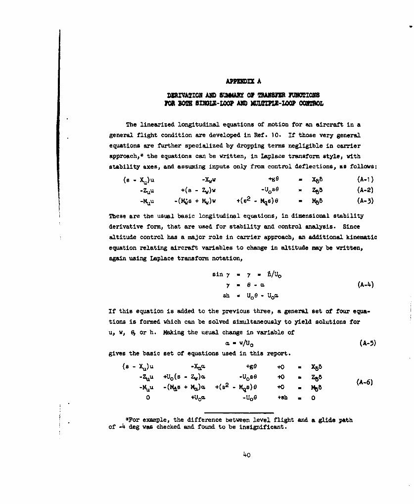
APPMIX A

DDZVATION AND SMOM OF UAIM FJUNCTIONSm0a 1 BnIaL-L00P AIM MUfLMI -LOP 030L

The linearized longitudinal equations of motion for an aircraft in ageneral flight condition are developed in Ref. 10. If those very general

equations are further specialized by dropping terms negligible in carrier

approach,* the equations can be written, in Laplace transform style, with

stability axes, and assuming inputs only from control deflections, as follows:

(s - Xu)u -XWV 4ge 45 (A-1)

-Z7uu +(s - ZV)w -Uose Z88 (A-2)

-M•u -(Ns + Kd)w +(s2 - Ms)e M86 (A-3)

These are the usual basic longitudinal equations, in dimensional stability

derivative form, that are used for stability and control analysis. Since

altitude control has a major role in carrier approach, an additional kinematic

equation relating aircraft variables to change in altitude may be written,

again using Laplace transform notation,

sin y - y - fi/Uo

Y U e - M (A-li)

sh = Uoe - Uo.

If this equation is added to the previous three, a general set of four equa-

tions is formed which can be solved simultaneously to yield solutions for

u, w, , or h. Making the usual change in variable ofS= v/Uo (A-5)

gives the basic set of equations used in this report.

(s - Xu)u -xYjM +go +o x58

-Zuu +Uo(s - Zw)a -Uos6 +0 = z5 (A-6)-Mdu -(Mis + MM)cX +(82 _ Ms)e o - 68

0 +UoM -Use +sh - 0

*For example, the difference between level flight and a glide pathof -4 deg was checked and found to be insignificant.

40

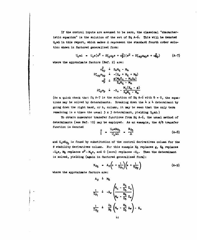
If the control inputs are assumed to be zero, the classical "character-

istic equation" is the solution of the set of Eq A-6. This will be denotedUosA in this report, which makes A represent the standard fourth order solu-tion shown in factored generalized form:

UoSL - UoS(S 2 + 2%pas + af)(s 2 + 2 tspwsps + Gp) (A-7)

where the approximate factors (Ref. 2) are:

2 -

GDsp Z'- -• Mq2 tspwsp -i(Z + Mq + M&)

g(MZu - MuZ,)

ZwMq -Mai

MX- i (,- g)

(As a quick check that Zq A-7 is the solution of Eq A-6 with 5 - 0, the equa-

tions may be solved by determinants. Breaking down the 4 x 4 determinant by

going down the right hand, or h, column, it may be seen that the only term

remaining is s times the usual 3 x 3 determinant, yielding Uoas.)

To obtain numerator transfer functions from Eq A-6, the usual method of

determinants (see Ref. 10) my be employed. As an example, the 9/5 transfer

function is denoted e UosNe5 _N__(A8

= %-os =S -A

and UosN9e is found by substitution of the control derivatives column for the

e stability derivatives column. For this example X8 replaces g, Ze replaces

-U0 S, M8 replaces 82- Mqs, and 0 (zero) replaces -Uo. Then the determinant

is solved, yielding (again in factored generalized form):

Neb- Ae( 3 T92s~L (A-9)

where the approximate factors are:

Ae "- M8

Tel

Te M - Z8 -X

41

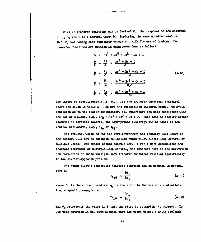
Similar transfer functions my be derived for the response of the aircraft

in u, m, and h to a control input 5. Employing the same notation used in

Ref. 2, but making each numerator consistent with the use of A alone, the

transfer functions are written in unfactored form as follows:

A As4 + Bs3 + Cs2 + Ds + E

e No As2 + Bs + CT 0 A

u Nu As3 + Bs2 + Cs + DS " A (A-1 )

S N=x As3 + Bs2 + Cs + D

h Nh As3 + Bs2 + Cs + D

The values of coefficients A, B, etc., for the transfer functions indicated

above are given in Table A-i, as are the appropriate factored forms. To avoid

confusion as to the proper denominator, all numerators are made consistent with

the use of A alone, e.g., sNh - As3 + Bs2 + Cs + D. Note that to specify either

elevator or throttle control, the appropriate subscript can be added to the

control derivative, e.g., Xke or XbT.

The results, which so far are straightforward and probably well known to

the reader, will now be extended to include human pilot closed-loop control of

multiple loops. The reader should consult Ref. 11 for a more generalized and

thorough treatment of multiple-loop control; the interest here is the derivation

and tabulation of those multiple-loop transfer functions relating specifically

to the carrier-approach problem.

The human pilot's controller transfer function can be denoted in general

f o r m b y M( 1

Y51q -(A-l)

where 81 is the control used and % is the error in the variable controlled.

A more specific example is

Y M e (A-12)

and 0. represents the error in 6 that the pilot is attempting to correct. To

use this notation it has been assumed that the pilot closes a unity feedback

42

++

tiCY

+u

++ ++ R E~

_C +

it

o Aco

++ n t

to -.

++ +4 ++

to IRb fCki+ + 0111ý-0 :e+

++

CIs

loop and his transfer function is called Yp, but note that this Yp is still

general in form. It can consist of any of the possible forms described in

Section II.

Deriving the pilot-controlled 6- Be system transfer function, Eq A-12

my be writtenbe = 8ee (A-1-)

6e - ec - e

and letting ec be defined as zero,

be = -YseGe (A-14)

Substituting the right side of Eq A-14 into Eq A-6 and collecting terms in e

gives

(s - Xu)U -X=M +(g + YbeX 8e)e +C - 0

-Zuu +Uo(s - ZW)a +(-Uos + Y5eezbe)e +0 = 0

-Muu -(Mas + MO)M +(s2 - Mqs + Y4eee)e 40 - 0

o +UoC -Uo9 +sh = 0

Rewriting Eq A-I 5 in matrix form and for convenience introducing the notation

aij for the coefficients of the motion quantities u, m, 9 results in

s.I al 2 a 13 + YbeeXbe 0 U

a21 Uoa2 a2 3 + Ybeeke 0 - 0 (A-16)a[ 1 a? a 33 + Y5 eo5e 0 a

L0 Uo -Uo J . h

This can be broken down, using the laws for determinants, into

a 1 a 1 2 al all a1 2 X8e

s a2 1 Uoa 2 2 a 2 , + Y~ 6 s a2 1 Uoa 2 2 Ze0 (A-17)

44

and this may be recognized as

Uos[A + Y e~ej a 0 (A- 18)

which is the closed-loop characteristic equation (i.e., closed-loop denominator)

of the open-loop transfer function

YbeeNe~e

A (A- 19)

(Note that the open-loop transfer function N(s)/A(s) has the closed-loop

transfer function N(s)/[A(s) + N(s)].) This my seem like a lot of effort to

prove what block diagram algebra would have shown immediately, namely that the

pilot transfer function multiplied by the airframe transfer function is the

system (open-loop) transfer function. However, the technique becomes useful

in deriving multiple-loop transfer functions by avoiding very complicated block

diagram breakdowns.

As an example, consider pilot control of airspeed with throttle and pitch

attitude with elevator. Making the appropriate pilot transfer function substi-

tutions, Eq A-6 in determinant form becomes

all + Y bub a1 2 a 1 3 + Y8eexre 0 u

a21 + YSVub Uoa 2 2 a 2 3 + Yee 0 0 (A-2)

a3 1 + YSTUl% a32 a33 + Ybele 0 e

0 Uo -Uo a h

Breaking this determinant down, it becomes (A-21)

a + a12 aa aY + 8 6al 1 12 a13 +Ye•e X8T a12 a1 + ee

s a2 1 Uoa2 a2 3 + Ybe68e + sY8Tu ZT Uo~a2 a2, + ¥beZe

a31 a, 2 a33 , Y+eee MeT a32 a33 + ¥eAe

45

The first determinant may be recognized as the one in Eq A-16, while the second

one may be further reduced to

XBT a 1 2 xbe

Uo5Y6TuNu5 + BY bTUY Y e T Uoa 2 2 Zb (A-22)

MB a32 Me

Introducing the notation

XbT a 1 2 X8 e

UoNue T Uoa 2 2 ZBe (A-23)

'%T a32 M~e

what this new determinant represents is the effect of control in one loop on

the zeros of the other loop-in other words, the control coupling between the

two loops. Notice that the notation employed suggests the replacement of the

u and 6 columns in the matrix equations of motion by the appropriate control

parameters in accordance with Eq A-23. Such replacement gives the appropriate

coupling transfer function whether the basic 3 x 3 or the augmented 4 x 4

matrix of Eq A-6 is utilized. Notice further that there is no coupling

between two variables being controlled with the same control (e.g.,N e h

To explain, if altitude and attitude are both being controlled with elevator,

the pilot in correcting altitude simply changes his commanded pitch attitude

so there is no coupling effect. This is borne out mathematically by noting

that if the elevator control derivatives were substituted in both the h and G

columns in Eq A-6, the solution of the determinant would be zero since any

determinant with two identical rows or columns is identically equal to zero.

The final closed-loop characteristic equation for the multiple-loop

control of u-4- T and G-ý 5e, or of Eq A-20, has now become

Uos + + Y uNur + Yb eY N ] - 0 (A-24)

46

There are two open-loop system transfer functions which can give this closed-

loop system, and these are

Yb.u(Nu8 + Yedu1

y 8T 8 (A-25)W O_ -3e be 6 + YBeoeb

YUee(Ne\ + Y5TuNgTie )A-6S(A-26)

"5ee be) -.3 6T - +YTuUBT

The notation on the left side of the equation denotes which loop is being con-sidered as the outer loop and which as the inner loop (e.g., in Eq A-25, G -3 be

is the inner loop).

The longitudinal coupling numerators have been derived and their

coefficients and factored forms are tabulated in Table A-2, taken from Ref. 11.(Note that the same convention is employed as in Table A-I, i.e., the term "A"

is the coefficient of the highest power in s and the last term is the coeffi-

cient of so, i.e., a constant.)

Now the previous two-loop pilot control result can be generalized by

considering potential control with five loops: e -: be; u -> be, 8T; h -0 be, 5T;or G --* be; Q -> be, &T; h -) be, BT. The closed-loop characteristic equation

can be written out by inspection, Just by sumiing the terms of the followingequations:

1. The aircraft characteristic equation A2. All of the single-loop numerators

3. All of the coupling numerators betweencontrol loops

Once the closed-loop equation is known, the open-loop equations for

appropriate controlled variables can be written by separating the numerator

and denominator terms for the open loop from the closed loop. As an eammple,

consider 9 --> be; u -0 be, BT; h -l be, 5T. The closed-loop characteristic

equation is

47

TABLE A-2LONGITUDINAL COUPLING NUMERATOR COMMICENTS AND FACTORED FORMS

A 3 C

W55 YT- Mqs. Mu1%XbT - b,~c)

Kzb*UT - 24~xbe) + Z,(XaQtT. xb4%)or

A~,( +~L

oro

uomebT4 -m( N6TZ)

or

or

or *1 )Z.I 2~

AO91r, h a L~T~~

S+ Y5eeNhb e + Y5 euNU e + Y6 TUYN gT

9 uhY6~5 O Y b'ZhNh8T + YbeuYbTpiN6T

+ YTuYehN e h 0 (A-27)

Three outer open-loop transfer functions can be written from this equation as

a function of various inner loop closures:

Yb A Ye( Nt6 e+ YBTUNU L + Ybh(A8"I 8 5e,5T A YbeuNu8 e + YSTU N UT+ YbehNh8e+ Yb~hNIT

uh e8h

YeuYbThNberJT + YbTJaYehN9T~e

(A-29)

Ybeu( NU~e+ 6 e)+ + sN e+ Y8ehN&TZe)

A) +* bee68 + + Y N +Y5Y Bh -0' BeA A + Ybe~e~ee + Ybe h~he 5T YahN8,_"T e+ W Ye6 TNeh._

h -+ 5e5hT

Y~eh (Nhbe + Y5TuIbTe) + Y bTh(NhsT e +h eebq3e)

h~e 8W e - '5 e 6 + YbeONese + Y¥euNub e + YBuTu5T + YseeYf3TUN8ebTu -30 beAT b ~

(A-30)

If angle of attack is being used instead of airspeed, the angle of attack

multiple-loop transfer functions can be obtained by substituting m for u in the

equations and multiplying Uo times all terms not containing an Q. If any loops

are not being used (e.g., no h -0 BT loop), the transfer functions of Eq A-28Io A-30 can be corrected by setting the corresponding Ybiq equal to zero for

the loops not being used.

49

A1TUIX 3

GINIRC PROPI=8 OF 813G01- AND =WJ -LON YZDMM CMMW

A. I1ZR0DUION

Examination of the transfer functions of a large number (ten) of aircraft

in power-approach configuration has revealed that they all have roughly the

same stability characteristics. This held true not only for a variety of single-

and multi-engine swept wing types but also for two tailless delta configurations

(the F7U-3 and F4D-]). The conclusion may be drawn that conventional aircraft

(i.e., not rotary wing, dynasoar, etc.) have the following general stability

properties in landing approach:

1. Phugoid frequency given approximately by the classical formulapý a 4g/Uo, which works out to a frequency of about 0.20 rad/secfor jet carrier approach speeds

2. Phugoid damping ratio is low, p - 0.10 ± 0.05. The differencebetween a damping ratio of 0.15 and 0.05 is insignificant fromthe standpoint of stabilization and control requirements, so

-p - 0.1 is representative of phugoid damping ratios

3. Short period frequency varies between 1 .0 and 3.0 rad/sec

4. Short period damping ratio is between 0.30 and 0.50 with 0.35 anaverage value

The primary differences between configurations that affect the transfer

functions are thrust line angle of attack and thrust line offset from the c.g.

These affect the throttle control stability derivatives ZB and Ma. respec-

tively, and also the airframe derivative Mu (see Ref. 10) and result in wide

variations of throttle control numerators between aircraft. Effects of these

variations will be considered where appropriate. The net conclusion reached,

however, is that even these possible variations do not change the generalities

listed above.

The discussion of single and multiple loop control systems is made with the

assumption that the reader has at least a working familiarity with servo analysis

'echniques. Most of the cases are illustrated by root locus diagrams although

50

an occasional Bode diagram is included. The purpose of this Appendix is a

technical justification of the rather sweeping allegations put forth in Section

III of the report, and therefore no attempt has been made to present the expla-

nations in terms other than those involving feedback control concepts.

B. AIRMM SINGLU-LOOP CO1OL CKRACTDXTIC5

The following discussion of single-loop control is intended to familiarize

the reader both with the general properties of airframe pole-zero locations in

landing approach configuration and with the effects of pilot loop-closure. It

is really preliminary to the more realistic multiple-loop systems examined in

the following subsection.

1. Pitch Attitude Control, e -1 be

The e - be single loop is fundamental to longitudinal control. The pilot's

primary reference to the horizon in VFR flight or to the vertical gyro in IFR

conditions attests to the importance and universal use by pilots of the pitch

attitude control loop. Being employed as an inner loop, the 8 -3 be closure

figures prominently in the minimum approach-speed criterion developed in

Section IV. The handling qualities of this control loop when evaluated for the

single-loop situation only (e.g., pitch attitude tracking) are dictated by the

short-period characteristics. Conversely, when employed in a multiple-loop

situation (e.g., where control of flight path is most important), then the

phugoid or long-term characteristics become dominant. It is therefore conveni-

ent to separate the high frequency and low frequency characteristics in analyzing

the 9 --i be properties as related to the carrier-approach problem:

Short-Period Characteristics (, The unequalized closure indi-

cated at the left in Fig. B-I shows a tendency for decreased closed-loop damp-

ing, top, a condition readily alleviated by the pilot's generation of a small

amount of lead equalization, TL; the right-hand part of Fig. B-I illustrates

the effect of a small TL. Therefore, if the open-loop (airframe alone) %~p and

tsp values are such that closed-loop damping in the order of Q0.35 is

achievable, the short-period characteristics are adequate for control during

carrier approach and do not require further consideration. (Such has been as-

sumed throughout this report.) It should be noted that the value of K9 is

selected by the pilot on the basis of attitude tracking requirements and the

51

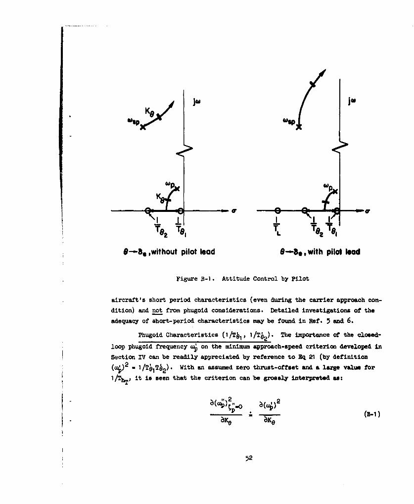
"spyjaipl jo

K9 JoJo

T82 Tel TIL8

9---. ,without pilot leoad 8-- , with pilot lead

Figure B-I. Attitude Control by Pilot

aircraft's short period characteristics (even during the carrier approach con-

dition) and not from phugoid considerations. Detailed investigations of the

adequacy of short-period characteristics may be found in Ref. 5 and 6.

Phugoid Characteristics (1 /Tb1 1/T92 ). The importance of the closed-

loop phugoid frequency uý on the minimum approach-speed criterion developed in

Section IV can be readily appreciated by reference to Eq 21 (by definition

(G)2 2 1 /T6 1TY2 ). With an assumed zero thrust-offset and a large value for

1 /Th• it is seen that the criterion can be grossly interpreted as:

9 6 - -(B-1)

52

p

The closed-loop frequency, w, is (from Eq 16)

I + K9

and partial differentiation yields:

Ke 0 TeI T2 (-2)

Therefore it is seen that for:

T1 > 1, increasing K0 results in increasedu)2TeTe2 >1 nraigK

1 < 1, increasing Ke results in decreased

w2TeTo2

(The parameter 1/c4 eiTe 2 is the static gain relative to the gain at the short

period, and was advanced in Ref. 5 as a possible source of control difficulty.

Also, the condition indicated by Eq B-2 corresponds to the speed for minimum

drag for the zero thrust-offset case-s___ee Ref. 5, Section V-c.)

The servoanalytic situation corresponding to Eq B-2 can be convenientlyillustrated by use of the Sigma-Bode plot (i.e., a - -a rather than the usual

s = jw), thoroughly explained in Ref. 17. For reasons which will become clearlater, assume that the only variable parameter in Eq B-2 is the time constant

1 AreI. For three selected value of 1 Ae 1 the corresponding Sigma plots are

shown in Fig. B-2. Note that the closed-loop roots, 1 t, 1/T81 , whose prod-uct is the closed-loop frequency, (SA) 2 , are uniquely defined by the intersec-

tion of the gain line and the curve WG(-o)I (see Ref. 4, 17). The condition ofsymmetry about u in Fig. B-2b renders the value of q insensitive to gainchanges. That is, increasing Ke increases 1 A 2 and decreases I/Tbi by the

same factor so that their product is unchanged.

In actual carrier approach-speed flight conditions, it was found that for

zero thrust offset 1/Tae was the only parameter that varied appreciably for

53

-0"--

(log scale) /

"Effect of increasing Ke:I/7 decreases slowly

1,'s increases moderately

K~a2 .g'wk'a ~ Increases

(slowly) as gain s iincreased

case b Shoed o.•cijterion shoed

Effect of increasing K1 :6 -d} //r decreases at some

'roat as l/7O; Increases

- *'-()• 2 - remains

constant as gain is varied

case c •oped less Mhencase_ ritron ii/ C Ioyý

- Wp

Effect of increasing KO:K_.-/•r; decreases rapidly

increases slowly

S(roAy) as gain is increased

Figure B-2. Sigm Bode Plot (s m -a) of the Phugoid Mode for Various Values of 1/Te1

54

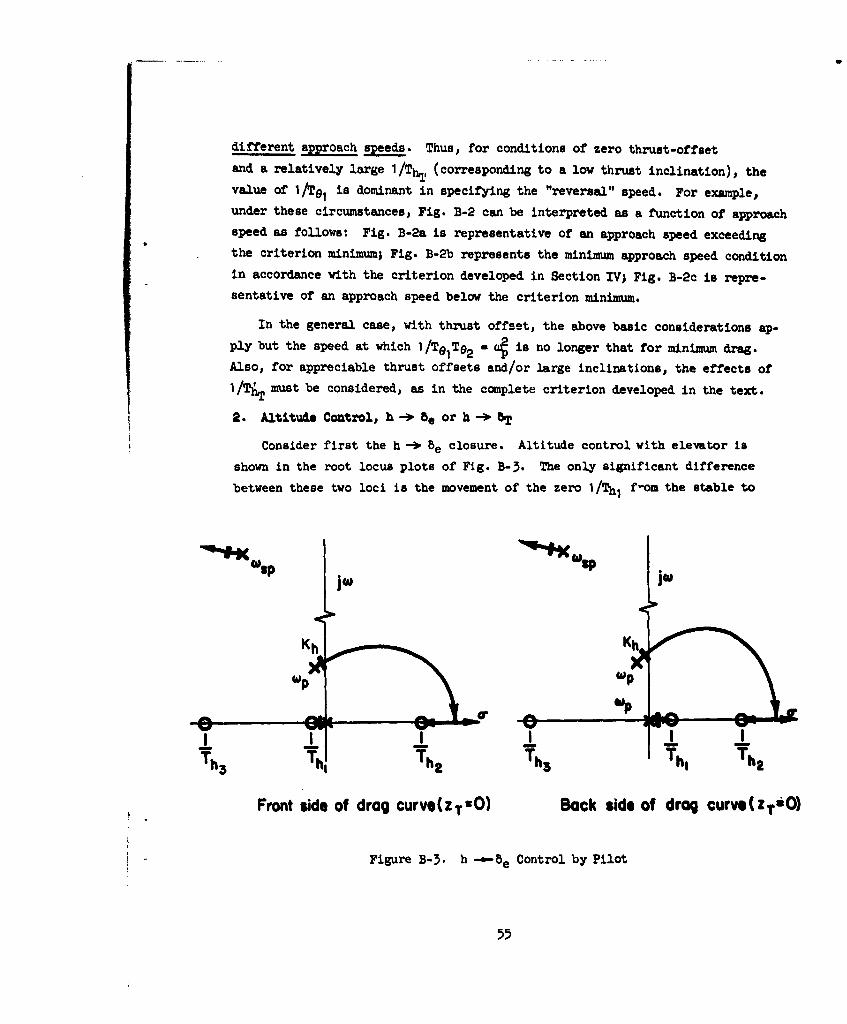
different approach speeds. Thus, for conditions of zero thrust-offset

and a relatively large 1/Th. (corresponding to a low thrust inclination), the

value of 1/T19 1 is dominant in specifying the "reversal" speed. For example,

under these circumstances, Fig. B-2 can be interpreted as a function of approach

speed as follows: Fig. B-2a is representative of an approach speed exceeding

the criterion minimum; Fig. B-2b represents the minimum approach speed condition

in accordance with the criterion developed in Section IV; Fig. B-2c is repre-sentative of an approach speed below the criterion minimum.

In the general case, with thrust offset, the above basic considerations ap-

ply but the speed at which 1/TelTe2 - 4 is no longer that for minimum drag.

Also, for appreciable thrust offsets and/or large inclinations, the effects of

1/TYT must be considered, as in the complete criterion developed in the text.

2. Altitude Control, h -4 be or h --> bT

Consider first the h -) be closure. Altitude control with elevator is

shown in the root locus plots of Fig. B-3. The only significant difference

between these two loci is the movement of the zero 1/Thj f-om the stable to

Kb K

± I II

T T Tb, T.

Front side of drag curva(ZT-O) BalCk side of dragl CUrvO(zt"O)

Figure B-3. h -be Control by Pilot

55

the unstable half-plane below minimum drag speed. This changes the system from

a stable one (at least at low gains) to one unstable for all gnins. Such

destabilizing motion of the time constant 1/Th1 an a function of approach speed

can be easily understood by referring to Ref. 2, Eq 6-28, which shows that for

zero thrust offset (zT - 0),

1 . dD

Thus the sign of I/Thl changes at the speed corresponding to dD/du - 0, or the

speed for minimum drag.

The effect of a thrust offset on the h -o be closure can be inferred from

examination of a more complete expression for 1/Thi (for example, see Ref. 1,

Table III-1 and Eq 6-25), and noting that (Ref. 10) the increment in 14U due to

eccentric thrust is

2 TzT (B-4)S~~Uo Iy ('•

The h -* 5T Closure. Altitude control with throttle is depicted in

Fig. B-4, again for the case of zero thrust line offset from the c.g. The

zeros near the short-period poles essentially cancel the short-period mode,

leaving the phugoid mode dominant. The locus shows that the phugoid frequency

Wh

i Figure B-li. h -• ST; Front and Back Side of the Drag Curve

56

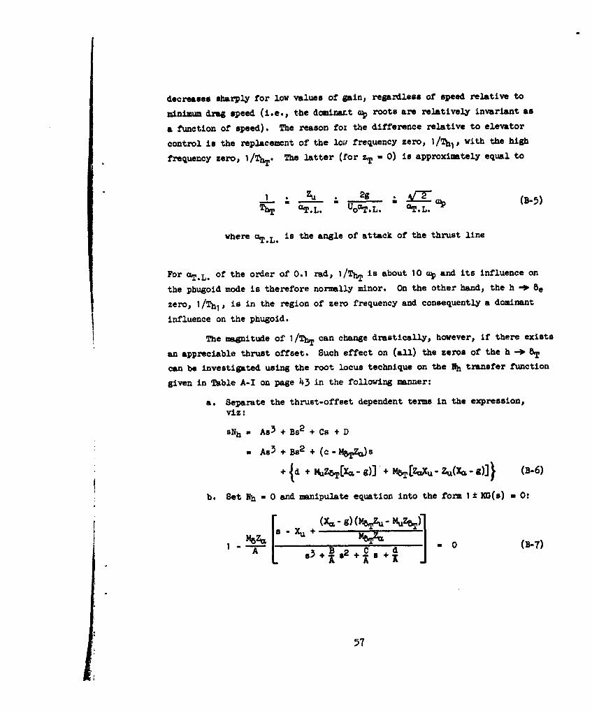
decreases sharply for low values of gain, regardless of speed relative to

minimum drag speed (i.e., the dominart ap roots are relatively invariant as

a function of speed). The reason fox the difference relative to elevator

control is the replacement of the loir frequency zero, 1/Thl, with the high

frequency zero,1 1/Th. The latter (for ZT - 0) is approximately equal to

- (3.5)r UThT aT.L. UoaT.L. OT.L.

where UT.L. is the angle of attack of the thrust line

For aT.L. of the order of 0.1 rad, 1/ThT is about 10 op and its influence on

the phugoid mode is therefore normally minor. On the other hand, the h -3 be

zero, I/Thj, is in the region of zero frequency and consequently a dominant

influence on the phugoid.

The magnitude of 1/ThT can change drastically, however, if there exists

an appreciable thrust offset. Such effect on (all) the zeros of the h -D 8T

can be investigated using the root locus technique on the Nh transfer function

given in Table A-I on page 43 in the following manner:

a. Separate the thrust-offset dependent terms in the expression,viz:

sNhu As3 + Bs2 + Cs + D

M As3 + 2 + (c _ %Zm)8

+ + )4ZBT :Xa- g)] + M8T [ZacxuZu(Xo.- )] (B-6)

b. Set Nh a 0 and manipulate equation into the form 1± KD(s) - 0:

1 [ Xus+ .... --- ] -(0

57

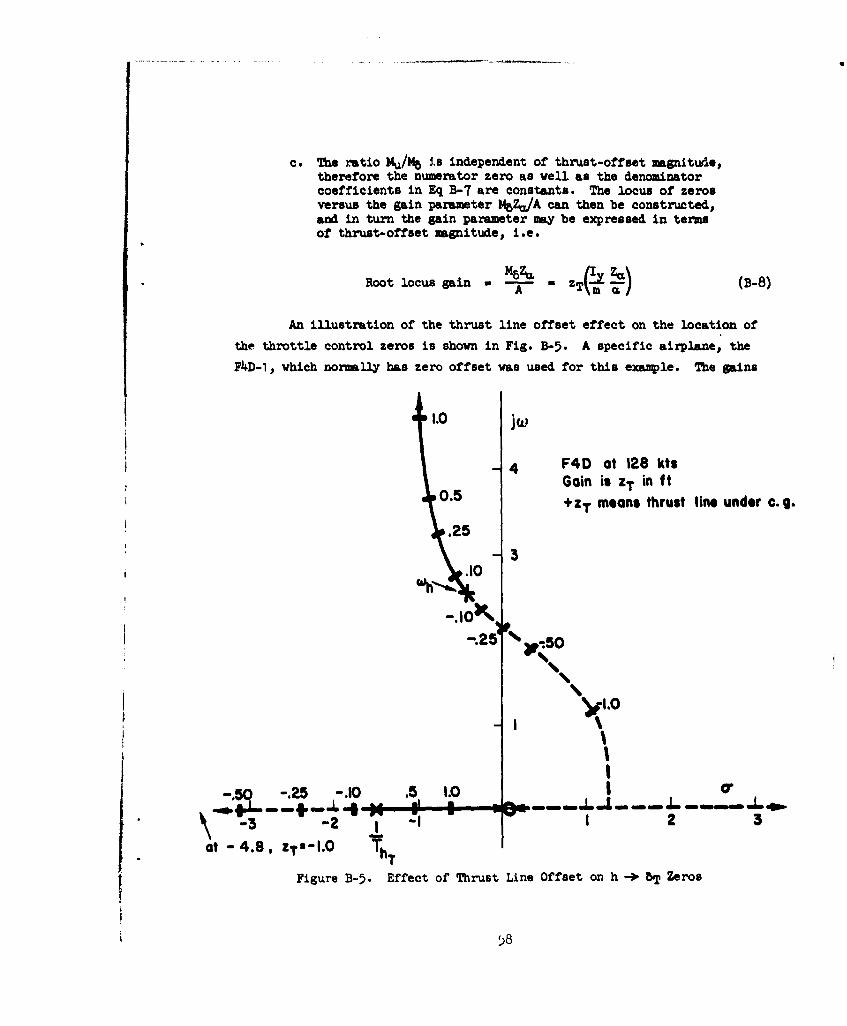
c. The ratio M4u/Mb is independent of thrust-offset magnitude,therefore the numerator zero as well as the denominatorcoefficients in Eq B-7 are constants. The locus of zerosversus the gain parameter MpZa/A can then be constructed,and in turn the gain parameter may be expressed in termsof thrust-offset magnitude, i.e.

Root locus gain - MA - Tm (B-8)

An illustration of the thrust line offset effect on the location of

the throttle control zeros is shown in Fig. B-5. A specific airplane, the

FAD-1, which normally has zero offset was used for this example. The gains

1.0 jCo

F4D at 128 kts0. Gain is ZT in ft0.5 +ZT means thrust line under c. g..25

I' 3.10

-.25%

-.50 -.25 -.10 .5 1.0 5 0... 4 MI -t mul In mammaL" Ja m m~am Mm L 48

%-l,0 2 3

at - 4.8, ZT-1.0 ThT

Figure B-5. Effect of Thrust Line Offset on h -5 8 T Zeros

are given in feet of offset, positive meaning thrust line below the c.g.

and vice versa. Typical values of offset for actual aircraft are between

0 and 0.5 ft, which gives an idea of practical limits in Fig. B-5. Con-

ceivably, with sufficient thrust offset below the e.g. the root I/Th can

exert some influence on the phugoid mode. Such an influence can be signifi-

cant on the minimum approach speed criterion developed in Section IV, i.e.,

its effect on a(ca ) 2 /ýKq. The other interesting point is that with suffi-

ciently large values Of-zT, a closed-loop problem could exist at short-period

frequencies, especially for configurations with Csp < 0.35, because of the

negatively damped wh.

3.Airspeed Control, u -* be, or u -->5

Root loci for airspeed control are shown in Fig. B-6. The u -! bT example

is again for zero thrust offset. These ere usually low gain loops, so their

single-loop characteristics are not very significant when multiple-loop control

is considered. The primary influence of these loops in the multiple-feedback

control case is on the zeros of the system as will be discussed later. Both

loop closures add phugoid damping (short period is almost unchanged), but

u -b be will increase phugoid frequency while u -l 5T will decrease it. It

should be noted that both forms of speed control are trim functions in thenormal or usual piloting technique. Therefore the long-term characteristics

(phugoid) are most important to the pilot.

Ku,

Ku WP WP

;. ~-50I

SU! T'JT

Figure B-6. Speed Control Loops

59

The effect of thrust line offset on the throttle control zeros is shown

in Fig. B-7. This effect was similarly computed as in the h -I bT loop

previously described (Paragraph 2), employing also the F4D at 128 knots. As

opposed to the altitude feedback case, it is evident that the speed control

zeros are hardly affected.

jW

4 F4D at 128 ktsGain is feet of thrust offset,positive thrust line under c.g.

-1.0

+1.01.

/ 2

Figure B-7. Effect ¢f Thrust Offset on u 6T Zeros

4. AngUe of Attaok Control, m -3P be, or m -b- 5T

Angle of attack control is again a low gain loop (when closed by a pilot).

The root loci are shown in Fig. B-8. Two points should be made about this

feedback loop. The first is that it is primarily a short-period phenomenon,

since the open-loop phugoid mode takes place at constant angle of attack.

60

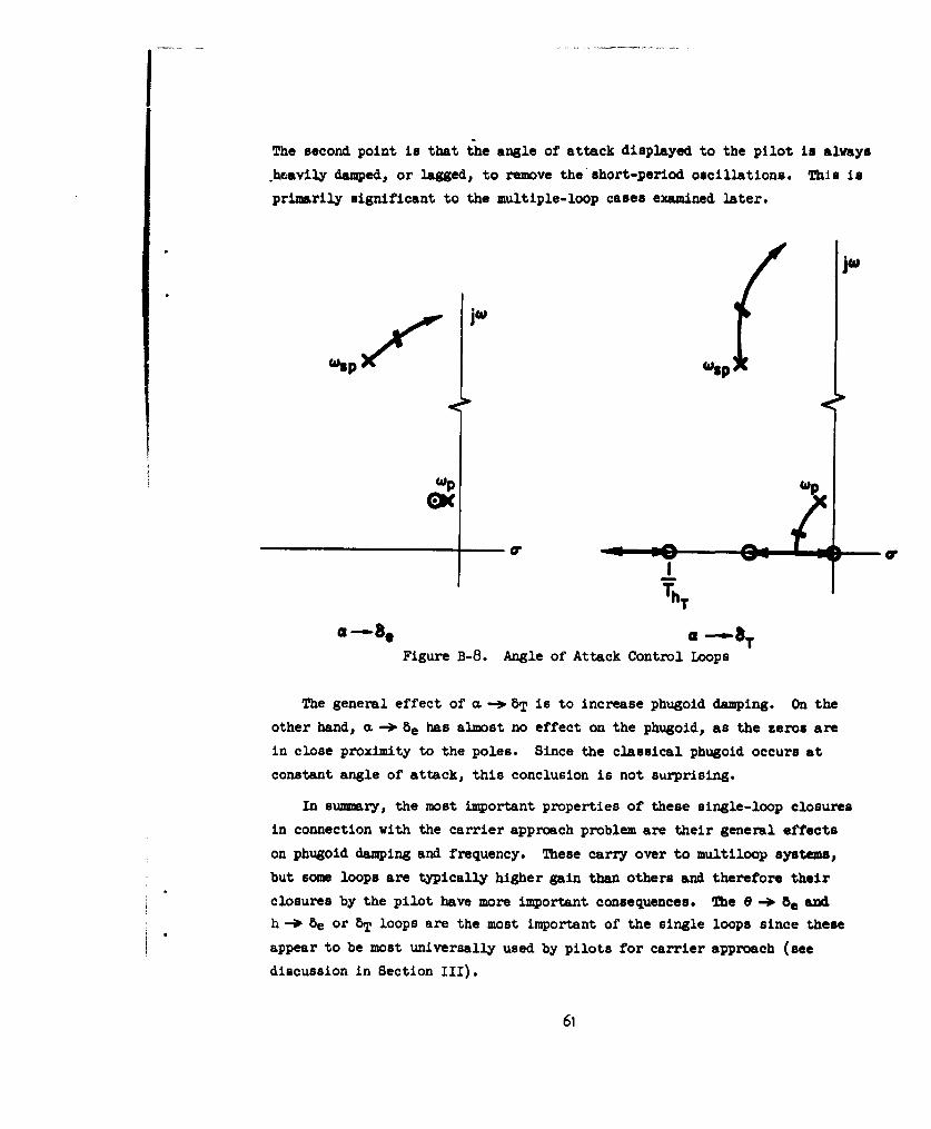
IThe second point is that the angle of attack displayed to the pilot is always

-hoavily damped, or lagged, to remove the short-period oscillations. This in

primarily significant to the multiple-loop cases examined later.

jo'

(ODP WA00I WWP

WP•pP

MIL

ThT

a ---8a T

Figure B-8. Angle of Attack Control Loops

The general effect of a -=i 5T is to increase phugoid damping. On the

other hand, m -i 8e has almost no effect on the phugoid, as the zeros are

in close proximity to the poles. Since the classical phugoid occurs at

constant angle of attack, this conclusion is not surprising.

In summary, the most important properties of these single-loop closures

in connection with the carrier approach problem are their general effects

on phugoid damping and frequency. These carry over to multiloop systems,

but some loops are typically higher gain than others and therefore their

closures by the pilot have more important consequences. The 9 -0 8 e nd

h -b 8e or bT loops are the most important of the single loops since these

appear to be most universally used by pilots for carrier approach (see

discussion in Section III).

61

C. MAWZPU-LOOP OWOM.L C1A08CTZCS

The intent of this subsection is to show generically how the results

described in Section III were obtained. The successive loop closures are

illustrated by root 'Loci for the three control techniques examined. No

specific numbers are used, the results being a generalization of specific

studies such as the one given in Appendix C. The three pilot control tech-

niques discussed in Section III are the ones examined here.

h. --• be, 0 --D- be, u. or c6-4-5

Altitude Response. Using the results from Appendix A, the open-loop

transfer function of elevator control of altitude, with e -4- be and u -3 bT

inner loops, is

The outer loop characteristic equation is found by summing the inner loop

transfer functions, which is the nmathematical process for closing the inner

loops. The sunintion process is as follows:

A + ybese 8 + Y qe) (5-10)

Y A' (B-11)

where A, is the closed-loop transfer function which results from closing the

6 "-• 8e loop. (Note that YbeSN8e/A in Eq 3-10 is the 6 --• 8e open-looptransfer function and (A + YthNe e) is the closed-loop equation.) This

e -p Te loop has already been discussed under single-loop control, in whichit was shown that the closure resulted in a wel-damped phugoid and a high

frequency short period. Therefore the root locus of this loop closure is

* the same as that in Fig. B-i.

62

Going now to the speed control loop, and for the time being neglecting

coupling between the e and u loops,

.T IT- ( + Y b~u~lub) (B-12)

The root locus for this loop is shown in Fig. B-9. The important point to

note is that this is a very low gain loop for reasonable values of pilot

throttle gain (see Appendix C). Therefore the aircraft's phugoid and short-

period characteristics are not appreciably changed by the pilot's throttle

movements to control airspeed. But as is shown later, this closure does

have a very important (stabilizing) effect through the numerator couplingwith the h -g -e zeros (i.e., allowing stable flight on the back side of

the drag curve with h -)- e control).

SJo'

WP'

S• •~KU_ P

Figure B-9. Pilot Closure of the u 5T Loop

The final denominator loop is the coupling between e and u control.

( + + Y~eeYbug e (3-1 )

The method of closure is the same as before, and specific cases have shown

that this too is a low gain effect, so the final inner loop denominator

characteristics are very close to those given by the e -* be single-loop

closure. This illustrates the great importance of pilot closure of the 8 loop.

The altitude control zeros are changed only by the coupling with the

u -> 5T loop. From the numerator of Eq B-9,

Nh5e + Y bpuNu - N=8e I+ 11hUe (B-14)

a Nhe

Closure of the loop denoted by the terms in the bracket is depicted in

Fig. B-10. It is seen that the primary effect is to stabilize the altitude

control zero, I/Thl, which is in the unstable half plane when the aircraft

is on the back side of the drag curve. For speeds above minimum drag, this

effect is unnecessary, therefore the u-* 8qT closure is redundant and not

required for altitude control.

|W

L KU

T3Th, Th2t2

Figure B-10. Effect of u-- 8T on h-> be Zeros

The underlying reason for this stabilizing effect is that the pilot

gain in the u-* 5T loop modifies the Xu equivalent stability derivative.

From Ref. 2, the approximate value for 1/Thl in terms of stability derivatives

is

64

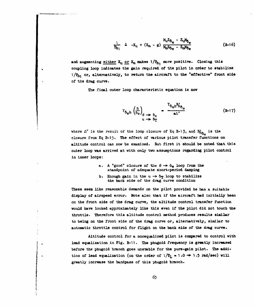
-X X,,-g)Mze -UM0(B-1 6)Th "-b -X + - de

and augmenting either Xu or XY makes 1/Thl more positive. Closing this

coupling loop indicates the gain required of the pilot in order to stabilize

I /%, or, alternatively, to return the aircraft to the "effective" front side

of the drag curve.

The final outer loop characteristic equation is now

I/h\ behh85I beh Ve-11 e (B- 17)

where A" is the result of the loop closure of Eq B-13, and N5Ae is the

closure from Eq B-15. The effect of various pilot transfer functions on

altitude control can now be examined. But first it should be noted that this

outer loop was arrived at with only two assumptions regarding pilot control

in inner loops:

a. A "good" closure of the e --3 8e loop from thestandpoint of adequate short-period damping

b. Enough gain in the u --> ST loop to stabilizethe back side of the drag curve condition

These seem like reasonable demands on the pilot provided he has a suitable

display of airspeed error. Note also that if the aircraft had initially been

on the front side of the drag curve, the altitude control transfer function

would have looked approximately like this even if the pilot did not touch the

throttle. Therefore this altitude control method produces results similar

to being on the front side of the drag curve or, alternatively, similar to

automatic throttle control for flight on the back side of the drag curve.

Altitude control for a nonequalized pilot is compared to control with

lead equalization in Fig. B-11. The phugoid frequency is greatly increased

before the phugoid branch goes unstable for the pure-gain pilot. The addi-

tion of lead equalization (on the order of I/TL - 1.0 -> 1.5 rad/sec) will

greatly increase the bandpass of this phugoid branch.

65

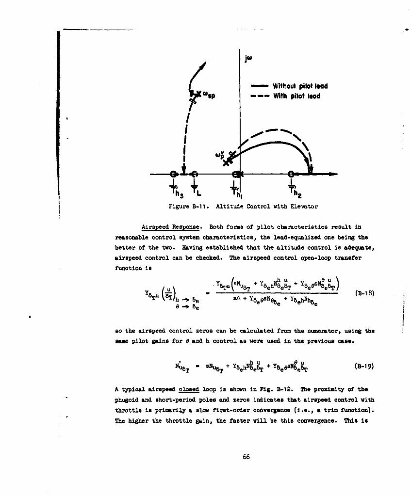
jO)

-- Without pilot leadp - -With pilot lead

IA -IL

Figure B-I I. Altitude Control with Elevator

Airspeed Response. Both forms of pilot characteristics result in

reasonable control system characteristics, the lead-equalized one being the

better of the two. Having established that the altitude control is adequate,

airspeed control can be checked. The airspeed control open-loop transfer

function is

Y ST N u5 +e Y s8T ( u (S =b beheBT e Y es bT) (B-18)

TU )h sBa + Y~eesfe5e + YbehNhbe

so the airspeed control zeros can be calculated from the numerator, using the

same pilot gains for e and h control as were used in the previous case.

,, SUb + Y8ehNe8T + Y UeasNVe (B-19)

A typical airspeed closed loop is shown in Fig. B-12. The proximity of the

phugoid and short-period poles and zeros indicates that airspeed control with

throttle is primarily a slow first-order convergence (i.e., a trim function).

The higher the throttle gain, the faster will be this convergence. This is

66

probably acceptable to the pilot if the airspeed disturbances are not too

severe. W.oC,

Th

s- Plans eWPC"Representation . Asymptotic Representation

0

Figure B-12. u -> 5T Closed Outer Loop

Angle of Attack Response. The altitude response with an m -o bT inner

loop is the same as with a u -- 5T inner loop if the gain is high enough to

stabilize the I/Thl divergent zero. Equation B-17 indicates that changing

either Xu or Xk will stabilize I/Thl.

The m -4 6T closed-loop zeros are positioned somewhat differently than

the airspeed zeros, however., as shown for a typical case in Fig. B-i3. .he

presence of a large residue (or distance) between the phugoid poles and zeros

indicates that a moderate phugoid oscillation will be present in the angle of

attack response. But the basic response is essentially similar to the u -b 8Tdiscussed previously.

S6PcLX

s-PlaneRepresentation PC1

€ T•hT

lad" Asymptotic Representation+h T "nhCL

Figure B;- 1. x -- 6T Closed Outer Loop

67

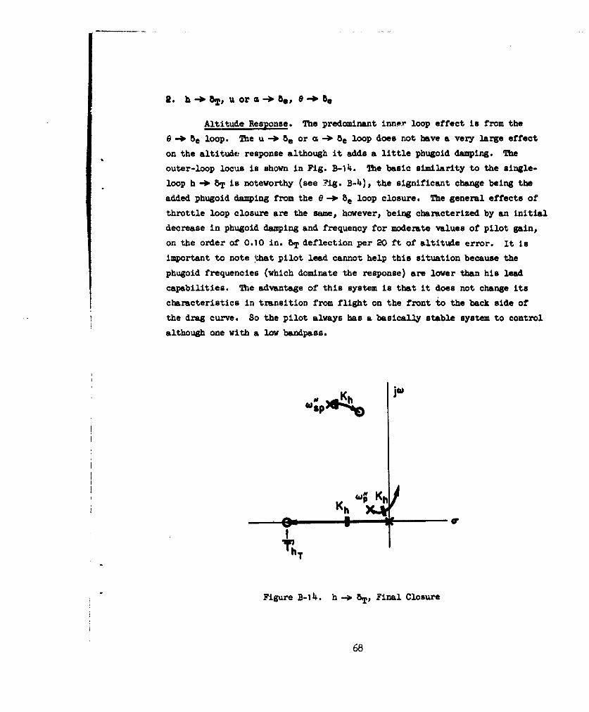
2. -)o T, uor a -)obe, e -. be

Altitude Response. The predominant inne.r loop effect is from the

S-b be loop. The u 8 e or c -'P 8e loop does riot have a very large effect

on the altitude response although it adds a little phugoid damping. The

outer-loop locus is shown in Fig. B-14. The basic similarity to the single-

loop h -) 5T is noteworthy (see ?ig. B-4)p the significant change being the

added phugoid damping from the 6 -P 5e loop closure. The general effects of

throttle loop closure are the same, however, being characterized by an initial

decrease in phugoid damping and frequency for moderate values of pilot gain,

on the order of 0.10 in. 5T deflection per 20 ft of altitude error. It is

important to note that pilot lead cannot help this situation because the

phugoid frequencies (which dominate the response) are lower than his lead

capabilities. The advantage of this system is that it does not change its

characteristics in transition from flight on the front to the back side of

the drag curve. So the pilot always has a basically stable system to control

although one with a low bandpass.

KhKh *

ThT

Figure B-14. h -8 8 T, Final Closure

68

Airspeed or Angle of Attack Response. The coupling between theh -) 5T inner loop and the u -0 be outer loop moves the outer-loop zeros to

a position as shown in Fig. B-15. This indicates that airspeed response is

stable but slow. Gust disturbances at frequencies higher than the

already low closed-loop phugoid cannot be followed quickly. Therefore speed

control will not be precise in turbulent air, but there will be no stability

problem. The pilot will probably accept this as inevitable rather than

attempt better control, since speed control is not as critical as altitude

control for a carrier landing and there is no way of improving the system

using this control technique.

SCL

Figure B-15. s-Plane Representation of Closed u-* be Outer Loop

Angle of attack response is quite similar in nature when the angle of

attack indicator is well damped to eliminate the short-period oscillations.

The dominant characteristic again will be the phugoid oscillation which is

low in frequency due to the h-> 8T loop.

69

APflNIZ C

A UMAIUID VAII OF W ANLIS T3CfI0J

The FAD-1 in power-approach configuration at an airspeed of 120 knots is

used for this example. The dimensional stability derivatives and aircraft

transfer functions are listed in Table C-1. The purpose of this appendix is

to illustrate how a series of loops are closed, how the gains for loop

closure are chosen, and finally how the resulting closed-loop system is

adjudged.

A. PILOT CON0TRL WITH 8 -- be, u -- 5T, h -- be

1. Altitude Control

The altitude control outer-loop transfer function, using Eq A-31 derived

in Appendix A and setting the terms Y5eu and YbTh to zero, is

2

[h ~ Ybeh(Nhbe + YbeuN5he)

[ 0] -3 be - Y5Tu(NeB + (c-i)k)U )-8T 8' + + +ý5

h be 1 -b

A convenient method for the solution of Eq C-i to render a factored polynomial

is to perform the additions, or loop closures, in the order indicated by the

brackets. The designated order is the proper sequence to give most insight

into the synthesis of the pilot's control functions and to minimize the number

of iterations in this process. Unfortunately there is no unique set or

sequence of operations which will accomplish this for general multiple-loop

control, but there are guidelines to govern this "art." The more pertinent

of such guidelines, fairly extensively treated in Ref. 11, are:

70

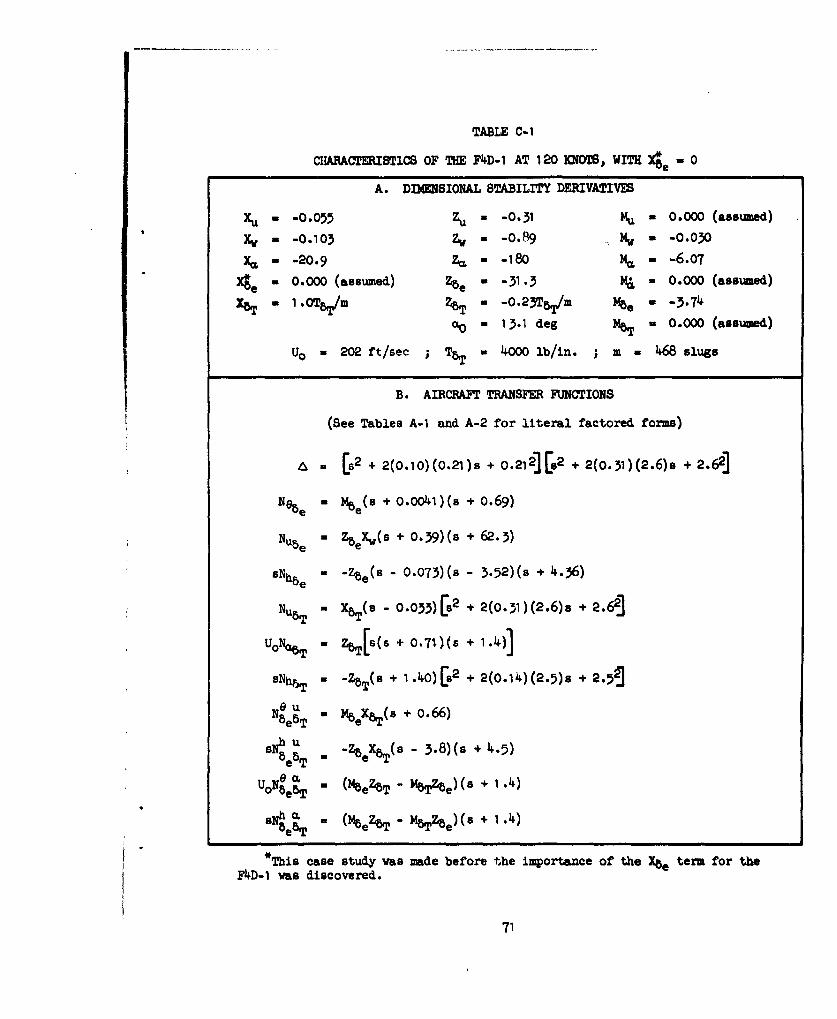
TABLE C-1

CHARACTERISTIC8 OF THE F4D-1 AT 120 KNOTS. WITH -e M 0

A. DDNSIONAL STABILITY DERIVATIVE

xu- -0.055 zu -0.31 M = 0.000 (assumed)

x. - -O.1O3 Z -o.89 MW - -o.o30

-= -20.9 - -180 M. - -6.07

4e- 0.000 (assumed) %e -31.3 M - 0.000 (assumed)

XTw1- O.TbT/m % - 0.23T&ý.m Me--37

-0 13.1 deg MTw 0.000 (assumed)

Uo = 202 ft/sec ; TBT 4.000 lb/in. ; m - 468 slugs

B. AIRCRAFT TRANSFER FUNCTIONS

(See Tables A-i and A-2 for literal factored forms)

A- [s2 + 2(0.10) (0.21)s + 0.212] [82 + 2(0- 31) (2.6)s + 2.62J

Nte - + 0. 0041 )(s + 0.69)

N ube - zbeXw(s + 0.39)(8 + 62.3)

SNhbe = -Zbe(s - 0.073)(s - 3.52)(s + 4.36)

N 8 . ( - o.o33)[s2 + 2(0.31)(2.6)s + 2.62]

UO0 T a BT[I(s + 0-71)(, + 1.)]

sNh a - - ( + 1.40)[s2 + 2(0.14)(2.5)s + 2.5•.

"a ,8T 1%eX8(s + 0.66)NeST e

U e8T - (eZ8r -u 3.8)(s + 4.5)

C'8e~ - M&

sNh .+ 4VT% (MeZbT - MBTZb)(, 8 •

*This case study was made before the importance of the te term for the

F4D-1 was discovered.

71

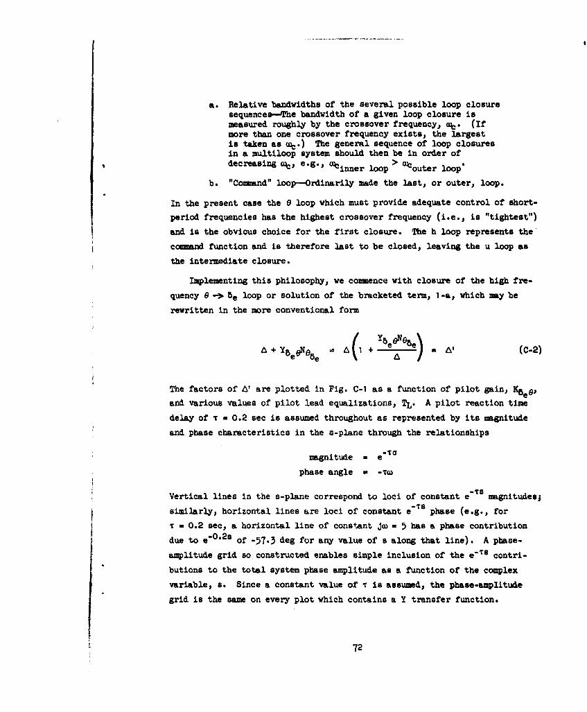
a. Relative bandwidths of the several possible loop closuresequences-The bandwidth of a given loop closure ismeasured roughly by the crossover frequency, ac. (Ifmore than one crossover frequency exists, the largestis taken as %o.) The general sequence of loop closuresin a multiloop system should then be in order ofdecreasing %o, e.g., ainner loop > 0couter loop*

b. "Command" loop--Ordinarily made the last, or outer, loop.

In the present case the 6 loop which must provide adequate control of short-

period frequencies has the highest crossover frequency (i.e., is "tightest")

and is the obvious choice for the first closure. The h loop represents the

ccmmand function and is therefore last to be closed, leaving the u loop as

the intermediate closure.

Implementing this philosophy, we commence with closure of the high fre-

quency 8 -> be loop or solution of the bracketed term, I-a, which may be

rewritten in the more conventional form

A + Y eNee A (I + C -2)

The factors of A' are plotted in Fig. C-1 as a function of pilot gain, K8ea,

and various values of pilot lead equalizations, TL. A pilot reaction time

delay of T u 0.2 see is assumed throughout as represented by its magnitude

and phase characteristics in the s-plane through the relationships

magnitude a e-To

phase angle a -Trw

-TsVertical lines in the s-plane correspond to loci of constant e magnitudes;

similarly, horizontal lines are loci of constant e"Ts phase (e.g., for

i w 0.2 sec, a horizontal line of constant jw a 5 has a phase contribution

due to e"0 .2s of -57.3 deg for any value of s along that line). A phase.

amplitude grid so constructed enables simple inclusion of the e-Ts contri-

butions to the total system phase amplitude as a function of the complex

variable, s. Since a constant value of T is assumed, the phase-amplitude

grid is the same on every plot which contains a Y transfer function.

72

R oots o, (4 + of) ./ 6

corresponding to KS, 1 '-1.16 rod/rod /x 2.9

/-0~~ 5

I 4I

/3&155

I"

\ -3

I'I

- ,

-2

alp

-6 -,-5 - 4 -3 -2 /-i/r

Fjgue C-I1 Closure of tiie Piloted e --> e LoOP

73

Assuming that desirable short-period control corresponds to a closed-loop

damping,•%p ? 0.35 (Ref. 5., 6 ), the required pilot lead equalization, 1/TLI

is approximately 1.5 as shown. Loop closure gain is then determined by inter-

section of the t - 0.35 radial with this selected short-period locus at the

highest frequency permitted (i.e., tightest control). Phugoid and reaction

delay closed-loop roots, u and 1/T9, are then specified by this gain value.Notice that the order of A' as given by the closed-loop roots (symbol 1)

shown in Fig. C-I is higher than that of A because of the additional I/'-r

first order. The corresponding factor, s + 1/T, is only a first approximation

to the closed-loop factors emanating from the open-loop e"1s because the

latter is transcendental in nature. If e"Ts, itself, is also approximated by

a single first-order factor, the 1/T'e factor is essentially cancelled. Toshow this, rewrite Eq-C-2 with NOeO given simply by e" 5s, i.e.,

-TS ~e1;SA + N085e(C3A' = + e 5 Ne8 e (c-3)eeTs

The numerator of the last expression to a first approximation contains the

factor s + 11/76, as in Fig. C-2. The denominator, to the same degree of

approximation, becomeseTS "- + s (s +,) (C-4)

For the value of r - 0.2 actually used, the cancellation is almost "exact" in

the case at hand.

The next closure (1-b) simply involves factoring since all the terms are

now specified. That is, substituting the numerators of Table C-1 and the Y5ee

equation determined from the previous closure into the 1-b bracket of Eq C-I

yields

Nu I + (-.374)(-1.16)e'0O2S(0.667s + M)(s + 0.66) (C-5)(s - 0.033)[B 2+ 2(0.31)(2.6)s + (2.6)9

The factors of Eq C-5 are computed by the conventional root locus technique

as is shown in Fig. C-2; the closed-loop poles, as denoted by I, are the

factors of Eq C-5. Here, again, the near-cancellation of the added 5+ I/b

factor as in the closure above will occur. Notice also that the root locus

74

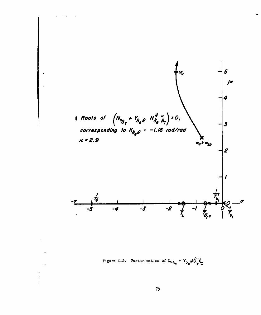
-5

4

IRoots of (a*Y 8 N9 00

corresponding to K -1.6 rad/rudxK#2.9,• w

2

-I

I T."

-5 -4 -3- I/ 0.

Figure C-2. Factorization of + 65eeT

75

gain, K, for this closure corresponds exactly to that of the previous closure

(Fig. C-I). Such correspondence holds approximately for all simultaneous

closures of multiple loops (Ref. 11) and exactly in the present cases, and is

an invaluable aid in conducting the loop closure sequence. It can easily be

checked by comparing the high frequency (i.e., s --* -) behavior of the open

loops. Thus, for example, for the closures indicated as 1-a and 1-b in Eq C-1

(values from Table C-1),

Y5 e 1NO5eI Y~eSMes 2 Y8 eOM~e

Closure I-a: Ye "is 1 - s4 8 2

Y N0uY5 Yb~XST Y5e A~Closure I-b: NUBeeT e( = XTS e 2e

__T XbTs3

Similarly, for closures 2 and 3,

Closure 2: T e T YbTu( ZbeBT -

Nh8e S -30 Za.s

Closure 3: YbTu(u8T + Ybe6bNe)e BT5 Y=TUX

'6 + Y5e~beS

Closure 2 is based on the stability problem associated with 6 -b 8e,

h --) be control and the remedying effects of the u -I BT loop which are

qualitatively described in Appendix B, Paragraphs A-2 and C-1, respectively.

Rewriting the bracketed numerator terms of Eq C-1 in a factored form and sub-

stituting values from Table C-1, we obtain the expression

Su +h I YbTu(XbT)(S - 3.8)(S + -4..6)

Nhbe + Y _TueU T Nhe ( (s- 0-073)(S- 3.52)(s +4.36) (c-6)

76

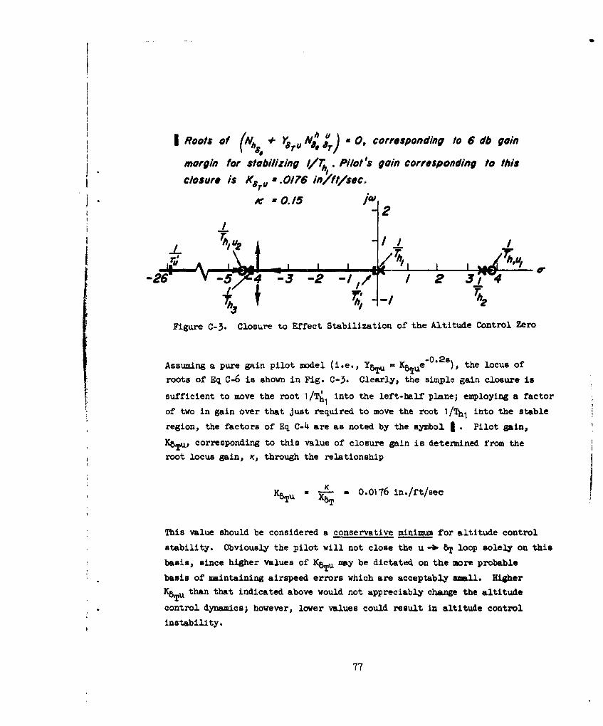
I Roots of Ali' You A ) a a, corresponding to 6 db goin

margin for stabilizing I/T/ . Pilot's gain corresponding to this

closure is Kg r .0176 in/ft/sec.•o Z .0. /5

h/ "2

Figure C-3. Closure to Effect Stabilization of the Altitude Control Zero

Assuming a pure gain pilot model (i.e., YbTu = KBTue' 0 "2 s), the locus of

roots of Eq C-6 is shown in Fig. C-3. Clearly) the simple gain closure is

sufficient to move the root I/Tý1 into the left-half plane; employing a factor

of two in gain over that Just required to move the root 1/Thn into the stable

region, the factors of Eq C-4 are as noted by the symbol I . Pilot gain,

KbTU, corresponding to this value of closure gain is determined from theroot locus gain, K, through the relationship

KbT - '0.0176 in./ft/sec

This value should be considered a conservative minimum for altitude control

stability. Obviously the pilot will not close the u -) T loop solely on thisbasis, since higher values of KbTu may be dictated on the more probable

basis of maintaining airspeed errors which are acceptably small. HigherK5Tu than that indicated above would not appreciably change the altitude

control dynamics; however, lower values could result in altitude control

instability.

77

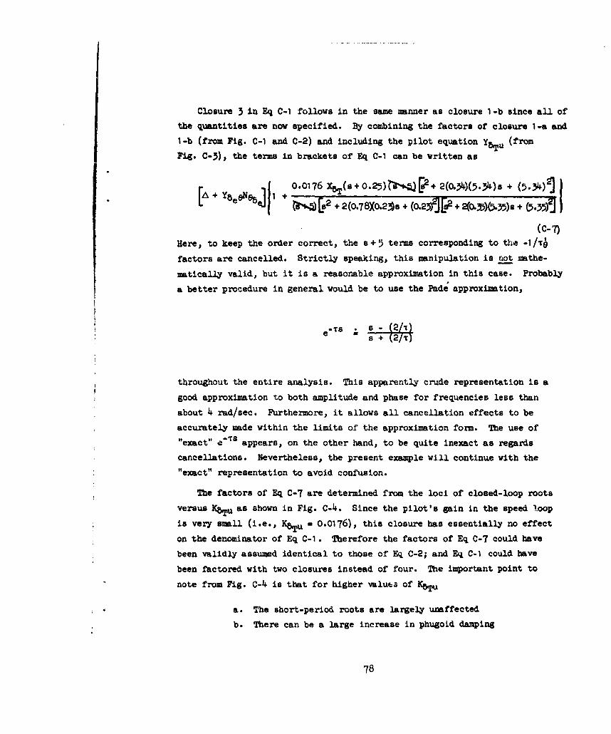
Closure 3 in Eq C-1 follows in the same manner as closure 1-b since all of

the quantities are now specified. By combining the factors of closure 1-a and

1-b (from Fig. C-1 and C-2) and including the pilot equation y8Tu (from

Fig. C-3), the terms in brackets of Eq C-1 can be written as

+ Y8ON&Q I +0.0176 X%(s+0.25)?r%4.Q.[s+ 2(0.34)(5.34)s +(539

e"%~ +2 2(0.78X0.2,js + (0.23)9pj + 2,C5"a+ (5.3.59

(c-7)Here, to keep the order correct, the s+5 terms corresponding to the -1/4

factors are cancelled. Strictly speaking, this manipulation is riot mathe-

matically valid, but it is a reasonable approximation in this case. Probably

a better procedure in general would be to use the Pade approximation,

T.S a s- ý2/ )e-s s + (2/T)

throughout the entire analysis. This apparently crude representation is a

* good approximation to both amplitude and phase for frequencies less than

about 4 rad/sec. Furthermore, it allows all cancellation effects to be

accurately made within the limits of the approximation form. The use of"exact" e-Ts appears, on the other hand, to be quite inexact as regards

cancellations. Nevertheless, the present example will continue with the"I"exact" representation to avoid confusion.

The factors of Eq C-7 are determined from the loci of closed-loop roots

versus KBTu as shown in Fig. C-4. Since the pilot's gain in the speed loop

is very small (i.e., K8Tu - 0.0176), this closure has essentially no effect

on the denominator of Eq C-1. Therefore the factors of Eq C-7 could have

been validly assumed identical to those of Eq C-2; and Eq C-I could have

been factored with two closures instead of four. The important point to

note from Fig. C-4 is that for higher valuea of Ku

a. The short-period roots are largely unaffected

b. There can be a large increase in phugoid damping

78

-5

jW

I Roots of 4

f4.YINI¶.Ya (Nu

for Y8 x 0.0/760e0°'h ; X 0.15

XRoots of -3

2

-26 -5 -4 -3 -2 -0 /-

Figure C-4. Effect of the Speed Control Loop Closureon the Altitude Control Denominator

Equation C-I can now be written in factored form from the root locations

found in Fig. C-3 and C-4.(C-8)

Y, -Z5,e (S,. + 0.075) (s -_3.6) (s + 4.4)rgQ

0 bee rS 2f [s2+ 2(0x.82,.1)s + (0..319 + 2(0.37X5h3-s + (5.302]u'' 5T

h-) be

Equation C-8 is the total open-loop h --> be control transfer function with

both e -> be and u -3 8'T loops closed. Altitude tracking performance is

79

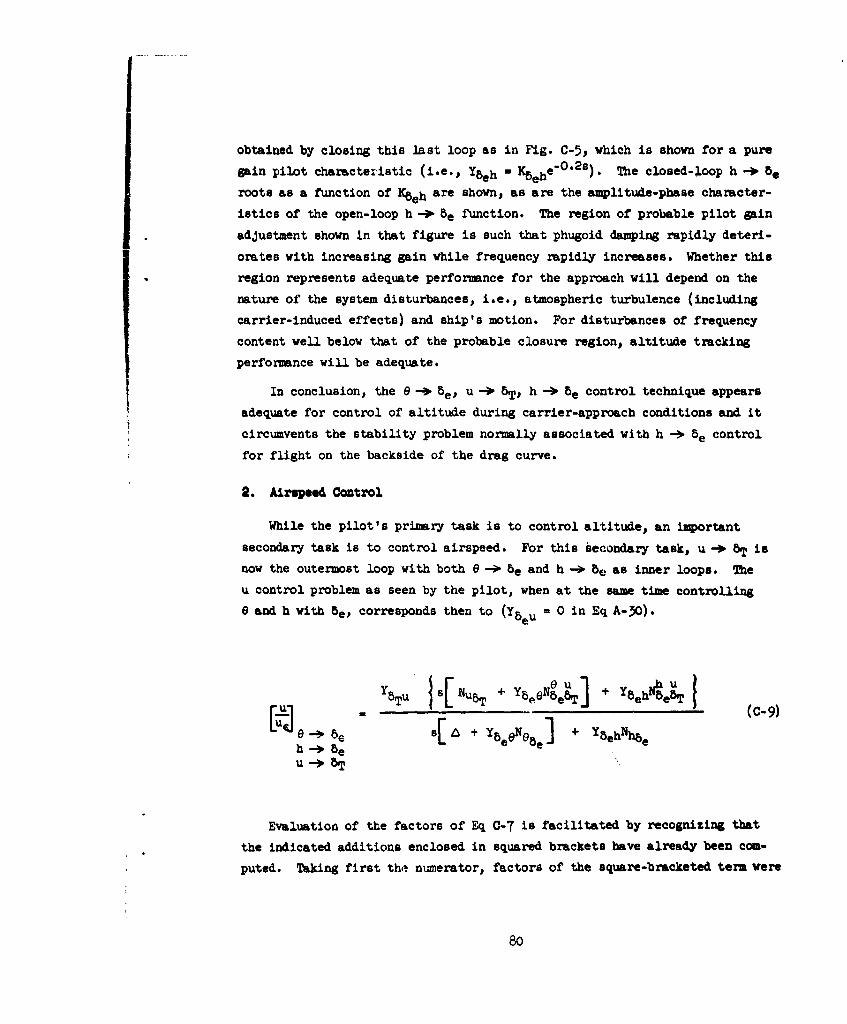
obtained by closing this last loop as in Fig. C-5, which is shown for a pure

gain pilot characteristic (i.e., Ybeh * KBehe' 0O 2 s). The closed-loop h -3 be

roots as a function of Kbeh are shown, as are the amplitude-phase character-

istics of the open-loop h -- be function. The region of probable pilot gain

adjustment shown in that figure is such that phugoid damping rapidly deteri-

orates with increasing gain while frequency rapidly increases. Whether this

region represents adequate performance for the approach will depend on the

nature of the system disturbances, i.e., atmospheric turbulence (including

carrier-induced effects) and ship's motion. For disturbances of frequency

content well below that of the probable closure region, altitude tracking

performance will be adequate.

In conclusion, the 6 --> 5ex u -0 6T, h --% be control technique appears

adequate for control of altitude during carrier-approach conditions and it

circumvents the stability problem normally associated with h -- Be control

for flight on the backside of the drag curve.

2. Airspeed Control

While the pilot's primary task is to control altitude, an important

secondary task is to control airspeed. For this secondary task, u-1 8T is

now the outermost loop with both e -0 be and h -> be as inner loops. The

u control problem as seen by the pilot, when at the same time controlling

e and h with be, corresponds then to (Y5eu = 0 in Eq A-30).

-A + Y,,N 0 8e + Y 8ehNhe

Evaluation of the factors of Eq C-7 is facilitated by recognizing that

the indicated additions enclosed in squared brackets have already been com-

puted. Taking first th'e numerator, factors of the square-bracketed term were

80

jdv tJ Proba.0/0 gain rolion of Pilof,a be Va/mOs. (Note that ,job

volues ar* negativ).

II I I W-5 -- 4 -3 -2 I 2 3 '4 5

/.3 Ke e-r($ + 0.075)(s - 3.6)(s f 4.4)

,L ,ifs'*•f2.82).3,, s +. (,/f,7/'# 2(5737).3(5 . 58).sY

Amplitude - Phase Characteristics

log W

- -db line fort '0..35probalGain 1Region 0db line for 4.0

Asymptotic/Y(s)/

60 db/decode-900

-/800 i W

F lmpire C-5. Altitude Control wit.h 6 --* Beg u -0. 8T Inner Loops Closed

81

determined previously in Fig. C-2; these factors are combined with the remain-

ing term through the root locus technique in Fig. C-6, yielding the complete

numerator factors as shown. Note that the gain variable of the locus is Keh

and the value selected for closure is that consistent with Fig. C-5 for a-" 0.•5.

The denominator factors of Eq C-9 are similarly determined. The factors

of the square-bracketed term were determined in Fig. C-1 and when combined with

the remaining term, as is done in Fig. C-7, yield the denominator factors shown.

Note that the gain variable in Fig. C-7 is also Kbeh, and that the root locus

gain for the selected closure must be identical to that used in Fig. C-5 and C-6.

Collecting the factors from Fig. C-6 and C-7 yields the factored open-loop

u -3 T transfer function

r~ un Ys TUX8T [s2 + 2(O.44XO.275)s + (0.275)9j[82 +2(O.35)(5.3~4)s +( 5.35)2)1

Ltd e be "T 1-°'02)6"*[s2+ 2(o.3)(o.4'6s + (o.4-'h9[s2+ 2(o.36)(5.4)s + (5J4)juh-30 5eh .--, 8 (C-la)

The significant dynamic characteristics shown in Eq C-10 very nearly reduce to

the easily controlled element K/s. The pilot accordingly should find closure

of the speed loop a very simple task.

For that value of Kb,, assumed to stabilize altitude control, the closed-loop characteristic factors of the speed loop must be identical to those of

the altitude loop computed previously in Fig. C-5. (Note that the closed-loop

u -. 5T denominator, given by the suammtion of open-loop numerator and denomi-

nator terms in Eq C-9, is identical to the similarly computed closed-loop

h -- 5e denominator from Eq C-i.) The closed-loop speed control equation can

therefore be written directly by collecting the numerator and denominator

factors from Fig. C-6 and C-5, respectively, which gives the following

polynomial:

[6 2 +2(o.44)0.276 + (0.275)9 s 2 + 2(0.35)(5.34I)s + (-59.h e (s + O.025)[s + 2(O.36)(0.5)s + (0.5)2 + 2(O.375)(5.5)s + (5.5mJ

(cuB.T (C-11)

82

59

I Roots of 4

/S[Nu 2 # ap A a] gh 0'

for Y hASO 0 h021

Kae ,.051 rad/ft

Fioure C-6. Effect of the Altitude Cort'rol Loop Closureon ttie Airspeed Contwol NMunerator

e %~

4 t~

.t t ~ t

48

Closed-loop speed control is characterized by a slow first-order convergence,

indicating that the selected value of K5Tu could have been made larger. Since

a higher speed loop gain improves both altitude and airspeed tracking, the next

logical step is to recompute the altitude and airspeed closed-loop dynamics with

a higher KbTu. Such a reiteration process, while worthwhile from the standpointof optimized design, is not necessary to reach the over-all conclusions:

a. For the minimum airspeed loop gain assumed to stabilizealtitude tracking, adequate altitude control results,and the speed loop is stable-but very sluggish.

b. For higher airspeed loop gains better altitude band-widths result and afford a much faster respondingairspeed control.

c. The assumed piloting technique provides adequate controlfor carrier approach of the FAD airplane regardless offlight speeds above or below that of minimum drag,although the speed loop closure is not required forspeeds above that of minimum drag.

B. PILOT 001ROL WITH -) be, h - e, a --3T

The previous example shows that good system characteristics are achievable

with throttle control of airspeed. But current Naval practice is to use angle

of attack rather than airspeed as a measure of the approach situation which is

less subject to variations due to weight and external configuration. It is

therefore pertinent to examine the use of m -0- BT (rather than u -- 5T) as an

alternative technique. As will be shown below, . -*. 5T for proper instrument

dynamics is essentially equivalent to u --> BT and there is no essential dif-

ference between these feedbacks, assuming both are equally accessible to the

pilot.

Because control of the phugoid appears to be the central problem inproperly executing the approach, angle of attack fluctuations at short-period

frequency must be damped or lagged out of the a display. In effect the aT

dynamics as displayed must be similar to those of u5T. This requirement is

also consistent with the use of the m reading as an indication of trim speed,i.e., steady state, not fluctuating, angle of attack information is desired.

Normally, then, filtering of the short-period a response is provided in the

indicator itself. The effect of this filtering is to make the m indicator an

equivalent airspeed indicator calibrated in degrees instead of knots. The

only difference, then, between the m -- 5T and u -- 5T as ar, inner stabilizing

loop in the required minimum gain for stabilizing the h -I 5e closure.

Paralleling the procedure adopted previously, the a -* 8 T closure gain require-

ment is computed below.

The altitude control numerator with 8 --> be and a -I 8T as inner loops can

be derived from Appendix A and is stated as Eq C-11.

Recalling from the previous example that for stable altitude control non-negative low frequency numerator zeros are not permissible, sets the gain term

of YbT,. The roots of Eq C-11 versus the pilot's gain Ka.. (assuming that

y j -0.2s) are shown in Fig. C-8. Again using a gain twice that

I Roots of foNh Y.STU Nb ],_ twice

ehe gain required to stabilize I// ,f, I' 1.2

-5 -4 -3-2 25

i Ti

-22I /-/

Figure C-8. Effect of -l 8T on Altitude Control Zeros

86

required to move the root I /TI into the left-half plane, the resulting closure

corresponds to a root locus gain of K a -1 .2. The required minimum pilot gain

can then be computed from the relationship:

K.K beze T ?48~z~) (C-12)

Substituting values from Table C-I and the specified root locus gain, we

obtain

Kr)TML (7-d)(57. eg/rad)

= -0.089 in./deg

Since a one-degree change in angle of attack correspondingly changes the

trim speed of the F4D-1 approximately four knots, the required throttle motion

in tracking angle of attack is approximately equal to that in tracking airspeed

for equal errors in airspeed.

In conclusion, the angle of attack indicator my be substituted for the

airspeed indicator to produce results comparable to the S -w be, u -3 T., h -i be

control technique described previously.

87