a swmm-5 model of a denitrifying bioretention system to
TRANSCRIPT

University of South Florida University of South Florida
Scholar Commons Scholar Commons
Graduate Theses and Dissertations Graduate School
2011
A SWMM-5 Model of a Denitrifying Bioretention System to A SWMM-5 Model of a Denitrifying Bioretention System to
Estimate Nitrogen Removal From Stormwater Runoff Estimate Nitrogen Removal From Stormwater Runoff
Michelle D. Masi University of South Florida, [email protected]
Follow this and additional works at: https://scholarcommons.usf.edu/etd
Part of the American Studies Commons, and the Environmental Engineering Commons
Scholar Commons Citation Scholar Commons Citation Masi, Michelle D., "A SWMM-5 Model of a Denitrifying Bioretention System to Estimate Nitrogen Removal From Stormwater Runoff" (2011). Graduate Theses and Dissertations. https://scholarcommons.usf.edu/etd/3237
This Thesis is brought to you for free and open access by the Graduate School at Scholar Commons. It has been accepted for inclusion in Graduate Theses and Dissertations by an authorized administrator of Scholar Commons. For more information, please contact [email protected].

A SWMM-5 Model of a Denitrifying Bioretention System to Estimate Nitrogen Removal
From Stormwater Runoff
by
Michelle Masi
A thesis submitted in partial fulfillment
of the requirements for the degree of
Master of Science
in Engineering Science
Department of Civil and Environmental Engineering
College of Engineering
University of South Florida
Major Professor: Sarina Ergas, Ph.D.
Jeffrey Cunningham, Ph.D.
Daniel Yeh, Ph.D.
Date of Approval:
November 2, 2011
Keywords: low impact development, hydrologic impact, nitrification, denitrification,
wood chips
Copyright © 2011, Michelle Masi

Acknowledgements
I would like to express my utmost gratitude to those who have guided me
throughout the design and implementation of this project. Although I have had countless
influences while conducting this research, I would like to explicitly thank the following:
Dr. Sarina Ergas for her continued support, advice, and ideas; committee members Dr.
Daniel Yeh and Dr. Jeffrey Cunningham for their insightful comments; the Charlotte
County Health Department and the FDEP Southwest District Office for their support and
flexibility; Mr. Thomas Lynn for his expertise, insight, training and patience; Mr. Steve
Heppler for his opinions, humor, and input; Mr. Jack Merriam from the Sarasota County
Environmental Management Department for providing low impact development project
information; my husband for providing encouragement; and my friends and family, who
have kindly provided countless hours of babysitting and support. You have all made my
dreams a reality; and I am so thankful to each and every one of you.

i
Table of Contents
List of Tables .................................................................................................................... iii
List of Figures .................................................................................................................... vi v
List of Acronyms .............................................................................................................. xii vi
List of Symbols ................................................................................................................ xiii
Abstract ............................................................................................................................ xiv vii
Chapter One: Introduction ...................................................................................................1 3
Research Objectives .................................................................................................4
Scope of Work .........................................................................................................5 1
Chapter Two: Background ...................................................................................................7 3
The Nitrogen Cycle ..................................................................................................7
Hazards Associated with Excess Nitrogen in Stormwater Runoff ........................12 3
Stormwater Management: Low Impact Development Technologies ....................15 9
Environmental Considerations for Implementing LID in SWFL ..........................25
Implementation of LID Technologies in Southwest FL .......................................29 15
Modeling an Alternative Bioretention System ......................................................32
State and Local Regulations...................................................................................33
Chapter Three: SWMM-5 Capabilities ..............................................................................34 29
SWMM-5 Software ...............................................................................................34
SWMM-5 Compartments.......................................................................................36 15
Atmospheric Compartment ........................................................................36 31
Land/Subcatchment Compartment .............................................................36 Maintenance Requirements for Bioretention Cells in SWFL 41 Practical Approa
Storage Unit ...............................................................................................37
Computational Capabilities ....................................................................................38
Horton Infiltration Method ........................................................................38
Curve Number Infiltration Method ............................................................39
Green-Ampt Infiltration Method................................................................39
Modeling Treatment with SWMM-5 .....................................................................39
LID Components ....................................................................................................40
Chapter Four: Site Characteristics .....................................................................................41 43
ii
Physical Characteristics .........................................................................................41 3
Proposed Bioretention System Design...................................................................43
Runoff Characteristics ...........................................................................................44
Chapter Five: Methods .......................................................................................................46
Phase I: Site-Specific Nutrient Characterization ...................................................46
Conceptual Model Development ...........................................................................48
Phase II: Analytical Bioretention System Model...................................................51
Phase III: Hydrologic ABC Model ........................................................................53
Phase IV: Water Quality ABC Model ...................................................................62
Chapter Six: Results and Discussion .................................................................................66
Phase I: Site-Specific Nutrient Characterization Results.......................................66
Phase II: Analytical Bioretention System Model Results ......................................67
Phase III: Hydrologic ABC Model Results ...........................................................68
Phase IV: Water Quality ABC Model Results .......................................................71
Chapter Seven: Conclusions ..............................................................................................79
Suggestions for Future Research ...........................................................................81
List of References .............................................................................................................82
Appendices ....................................................................................................... 89 Appendix A: Runoff Quality Analyses for Events #1 & 2 ....................................90
Appendix B: Extra Tables ......................................................................................94
Appendix C: SWMM-5 Input Parameters .............................................................95
Appendix D: SWMM-5 Water Quality Output Data ...........................................100
About the Author ................................................................................................... End Page #

iii
List of Tables
Table 1.1. Summary of LID technologies and their intended uses [adapted from
EPA, 2000] ........................................................................................ 4
Table 2.1. Summary of LID projects in southwest Florida................................................31
Table 3.1. General subcatchment characteristics as defined in SWMM-5
[adapted from Abi Aad et al. 2010] ...................................................... 35
Table 3.2. Principle input parameters needed to calibrate the SWMM-5 model for
this case study ................................................................................... 38
Table 4.1. Analytical methods summary and typical nutrient concentrations ...................45
Table 5.1. Four phases to develop the alternative bioretention cell model and the
purpose for each phase ....................................................................... 46
Table 5.2. Physical characteristics of the subcatchment [calculations are based
on Doyle and Miller, 1980; Tsihrintzis and Hamid, 1998] ...................... 57
Table 5.3. Storage unit and orifice input parameters (based on system designs
presented in Chapter 3). ...................................................................... 58
Table 5.4. Quantity input parameters [presented and verified by Tsihrintzis and
Hamid, 1998]..................................................................................... 60
Table 5.5. Model quantity calibration data: single-family residential site [based
on findings presented by Doyle and Miller, 1980]. ................................. 62
Table 5.6. Nitrogen species in runoff; used to calibrate the SWMM-5 model
[adapted from PBS&J, 2010 and field sampling data] ............................ 65
Table 6.1. Results of November 4th
and December 11th
, 2010 stormwater
runoff samples ................................................................................... 66
Table 6.2. SWMM-5 simulated pre-development TKN loading rates for six
separate storm events.......................................................................... 73
iv
Table 6.3. SWMM-5 simulated pre-development NO3--N loading rates for six
separate storm events.......................................................................... 73
Table 6.4. Simulated efficiency of nitrification in ABC models, for the six storm
events analyzed at the minimum nitrogen concentration. ........................ 74
Table 6.5. Simulated efficiency of nitrification in ABC models, for the six storm
events analyzed at the median nitrogen concentration. ........................... 74
Table 6.6. Simulated efficiency of nitrification in ABC models, for the six storm
events analyzed at the maximum nitrogen concentration. ....................... 75
Table 6.7. Simulated efficiency of nitrification in ABC models, for the six storm
events analyzed at the analyzed nitrogen concentration. ......................... 75
Table 6.8. Simulated efficiency of denitrification in ABC models, for the six
storm events analyzed at the minimum nitrogen concentration ................ 77
Table 6.9. Simulated efficiency of denitrification in ABC models, for the six
storm events analyzed at the median nitrogen concentration ................... 77
Table 6.10. Simulated efficiency of denitrification in ABC models, for the six
storm events analyzed at the maximum nitrogen concentration ............... 78
Table 6.11. Simulated efficiency of denitrification in ABC models, for the six
storm events analyzed at the analyzed nitrogen concentration ................. 78
Table A.1. TN analysis of stormwater runoff at Venice East Blvd. site ............................90
Table A.2. TP analysis of stormwater runoff at Venice East Blvd. site ............................90
Table A.3. pH analysis of stormwater runoff at Venice East Blvd. site ............................90
Table A.4. DO analysis of stormwater runoff at Venice East Blvd. site ...........................91
Table A.5. Turbidity analysis of stormwater runoff at Venice East Blvd. site ..................91
Table A.6. Conductivity analysis of stormwater runoff at Venice East Blvd. site ............91
Table A.7. BOD analysis of stormwater runoff at Venice East Blvd. site ........................92
Table A.8. TSS analysis of stormwater runoff at Venice East Blvd. site ..........................92
Table A.9. VSS analysis of stormwater runoff at Venice East Blvd. site..........................92

v
Table A.10. Total Coliform analysis of stormwater runoff at Venice East Blvd.
site ................................................................................................... 93
Table B.1. Comparison of long-term (1915-2010) rainfall data [adapted from
PBS&J, 2010] .................................................................................... 94

vi
List of Figures
Figure 1.1. Map of Florida; aerial map shows the exact location of
retrofit site [Google Maps, 2011]. ......................................................... 6
Figure 2.1. Pre-development vs. post-development hydrologic cycle
[Maryland DEP, 2010]. ....................................................................... 13
Figure 2.2. Depiction of the different layers found in a typical vegetated rooftop
[USEPA, 2010]. ................................................................................. 19
Figure 2.3. Stormwater runoff from a 3.35-inch green roof, during a 24-hour
[Roofscapes, Inc., 2000]. .................................................................... 19
Figure 2.4. Typical rain barrel setup, to collect stormwater runoff from a rooftop
[source: http://www.ci.berkeley.ca.us] .................................................. 21
Figure 2.5. Typical bioretention system [Prince George‟s County DEP, 1993]................22
Figure 2.6. Schematic of a conventional bioretention cell [MDE, 2000] ..........................23
Figure 2.7. Schematic of an alternative bioretention cell for treatment of nitrate
rich stormwater [Ergas et al., 2010] ............................................................24
Figure 2.8. Detailed map of Alligator Creek, located within the Lemon Bay
watershed [Sarasota County Wateratlas, 2010] ...........................................27
Figure 2.9. Florida Aquarium project depiction [Rushton, 1999].. ...................................31
Figure 4.1. Proposed location of cell thirteen, one of 13 bioretention cells planned
(outlined in red). ..........................................................................................42
Figure 4.2. Site plan of bioretention cell 13 [plans provided by Sarasota County].. .........43
Figure 5.1. Conceptual model framework .........................................................................50
Figure 5.2. SWMM 5.0.22 Model of alternative bioretention cell (ABC) ........................55
vii
Figure 6.1. Flow through the orifice controlled system for a 4.37-in. simulated
storm event for system sized according to Sarasota‟s plans .......................69
Figure 6.2. Flow through the orifice controlled system for a 4.37-in. simulated
storm event in system sized according to USEPA guidelines .....................70
Figure 6.3. TKNeff and NO3-eff concentrations vs. time in Sarasota sized model ..............71
Figure 6.4. TKNeff and NO3-eff concentrations vs. time in EPA sized model ....................72
Figure C.1. Options dialog box input parameters ..............................................................95
Figure C.2. Evaporation input parameters .........................................................................95
Figure C.3. Raingages input parameters ............................................................................96
Figure C.4. Subcatchments input parameters ....................................................................96
Figure C.5. Subareas input parameters ..............................................................................96
Figure C.6. Infiltration input parameters ...........................................................................96
Figure C.7. Outfalls input parameters ................................................................................96
Figure C.8. Storage unit input parameters .........................................................................97
Figure C.9. Conduits input parameters ..............................................................................97
Figure C.10. Orifices input parameters ..............................................................................97
Figure C.11. Weirs input parameters .................................................................................97
Figure C.12. XSections input parameters ..........................................................................98
Figure C.13. Pollutants input parameters ...........................................................................98
Figure C.14. Landuses input parameters ............................................................................98
Figure C.15. Washoff input parameters .............................................................................98
Figure C.16. Treatment input parameters ..........................................................................99
Figure D.1. Simulation using minimum concentration in Sarasota sized ABC
model for the 1/13/74 storm event ............................................................100

viii
Figure D.2. Simulation using minimum concentration in EPA sized ABC
model for the 1/13/74 storm event ............................................................100
Figure D.3. Simulation using minimum concentration in Sarasota sized ABC
model for the 4/15/74 storm event ............................................................101
Figure D.4. Simulation using minimum concentration in EPA sized ABC
model for the 4/15/74 storm event ............................................................101
Figure D.5. Simulation using minimum concentration in Sarasota sized ABC
model for the 6/17/74 storm event ............................................................102
Figure D.6. Simulation using minimum concentration in EPA sized ABC
model for the 6/17/74 storm event ............................................................102
Figure D.7. Simulation using minimum concentration in Sarasota sized ABC
model for the 7/19/74 storm event ............................................................103
Figure D.8. Simulation using minimum concentration in EPA sized ABC
model for the 7/19/74 storm event ............................................................103
Figure D.9. Simulation using minimum concentration in Sarasota sized ABC
model for the 9/18/74 storm event ............................................................104
Figure D.10. Simulation using minimum concentration in EPA sized ABC
model for the 9/18/74 storm event ............................................................104
Figure D.11. Simulation using minimum concentration in Sarasota sized ABC
model for the 12/26/74 storm event ..........................................................105
Figure D.12. Simulation using minimum concentration in EPA sized ABC
model for the 12/26/74 storm event ..........................................................105
Figure D.13. Simulation using median concentration in Sarasota sized ABC
model for the 1/13/74 storm event ............................................................106
Figure D.14. Simulation using median concentration in EPA sized ABC
model for the 1/13/74 storm event ............................................................106
Figure D.15. Simulation using median concentration in Sarasota sized ABC
model for the 4/15/74 storm event ............................................................107
Figure D.16. Simulation using median concentration in EPA sized ABC
model for the 4/15/74 storm event ............................................................107

ix
Figure D.17. Simulation using median concentration in Sarasota sized ABC
model for the 6/17/74 storm event ............................................................108
Figure D.18. Simulation using median concentration in EPA sized ABC
model for the 6/17/74 storm event ............................................................108
Figure D.19. Simulation using median concentration in Sarasota sized ABC
model for the 7/19/74 storm event ............................................................109
Figure D.20. Simulation using median concentration in EPA sized ABC
model for the 7/19/74 storm event ............................................................109
Figure D.21. Simulation using median concentration in Sarasota sized ABC
model for the 9/18/74 storm event ............................................................110
Figure D.22. Simulation using median concentration in EPA sized ABC
model for the 9/18/74 storm event ............................................................110
Figure D.23. Simulation using median concentration in Sarasota sized ABC
model for the 12/26/74 storm event ..........................................................111
Figure D.24. Simulation using median concentration in EPA sized ABC
model for the 12/26/74 storm event ..........................................................111
Figure D.25. Simulation using maximum concentration in Sarasota sized ABC
model for the 1/13/74 storm event ............................................................112
Figure D.26. Simulation using maximum concentration in EPA sized ABC
model for the 1/13/74 storm event ............................................................112
Figure D.27. Simulation using maximum concentration in Sarasota sized ABC
model for the 4/15/74 storm event ............................................................113
Figure D.28. Simulation using maximum concentration in EPA sized ABC
model for the 4/15/74 storm event ............................................................113
Figure D.29. Simulation using maximum concentration in Sarasota sized ABC
model for the 6/17/74 storm event ............................................................114
Figure D.30. Simulation using maximum concentration in EPA sized ABC
model for the 6/17/74 storm event ............................................................114
Figure D.31. Simulation using maximum concentration in Sarasota sized ABC
model for the 7/19/74 storm event ............................................................115
x
Figure D.32. Simulation using maximum concentration in EPA sized ABC
model for the 7/19/74 storm event ............................................................115
Figure D.33. Simulation using maximum concentration in Sarasota sized ABC
model for the 9/18/74 storm event ............................................................116
Figure D.34. Simulation using maximum concentration in EPA sized ABC
model for the 9/18/74 storm event ............................................................116
Figure D.35. Simulation using maximum concentration in Sarasota sized ABC
model for the 12/26/74 storm event ..........................................................117
Figure D.36. Simulation using maximum concentration in EPA sized ABC
model for the 12/26/74 storm event ..........................................................117
Figure D.37. Simulation using analyzed concentration in Sarasota sized ABC
model for the 1/13/74 storm event ............................................................118
Figure D.38. Simulation using analyzed concentration in EPA sized ABC
model for the 1/13/74 storm event ............................................................118
Figure D.39. Simulation using analyzed concentration in Sarasota sized ABC
model for the 4/15/74 storm event ............................................................119
Figure D.40. Simulation using analyzed concentration in EPA sized ABC
model for the 4/15/74 storm event ............................................................119
Figure D.41. Simulation using analyzed concentration in Sarasota sized ABC
model for the 6/17/74 storm event ............................................................120
Figure D.42. Simulation using analyzed concentration in EPA sized ABC
model for the 6/17/74 storm event ............................................................120
Figure D.43. Simulation using analyzed concentration in Sarasota sized ABC
model for the 7/19/74 storm event ............................................................121
Figure D.44. Simulation using analyzed concentration in EPA sized ABC
model for the 7/19/74 storm event ............................................................121
Figure D.45. Simulation using analyzed concentration in Sarasota sized ABC
model for the 9/18/74 storm event ............................................................122
Figure D.46. Simulation using analyzed concentration in EPA sized ABC
model for the 9/18/74 storm event ............................................................122

xi
Figure D.47. Simulation using analyzed concentration in Sarasota sized ABC
model for the 12/26/74 storm event ..........................................................123
Figure D.48. Simulation using analyzed concentration in EPA sized ABC
model for the 12/26/74 storm event ..........................................................123

xii
List of Acronyms
BMPs best management practices
BOD biochemical oxygen demand
COD chemical oxygen demand
DO dissolved oxygen
LID low impact development
MCL maximum contaminant level
NOx nitrogen oxides
Org N organic nitrogen
SJWMD St. John‟s Water Management District
SWFWMD SW Florida Water Management District
SWMM5 Storm Water Management Model 5
TKN Total Kjeldahl Nitrogen
TN total nitrogen
TP total phosphorus
TSS total suspended solids
USDA United States Department of Agriculture
USEPA United States Environmental Protection
Agency
USGS United States Geological Survey
VSS volatile suspended solids
WQS water quality standards

xiii
List of Symbols
V volume of the cell ( )
influent TKN concentration (mg/L)
effluent TKN concentration (mg/L)
effluent nitrate concentration (mg/L)
influent nitrate concentration (mg/L)
Concentration of reacted TKNi (mg/L)
k1 and k2 rate of nitrification and denitrification,
respectively (1/T)
HRT1 and HRT2 hydraulic residence time (hours)

xiv
Abstract
This research estimates nitrogen removal from stormwater runoff using a
denitrifying bioretention system using the USEPA Storm Water Management Model
Version 5 (SWMM-5). SWMM-5 has been used to help planners make better decisions
since its development in 1971. A conventional bioretention system is a type of Low
Impact Development (LID) technology, which designed without a media layer
specifically for achieving nitrogen removal. More recently studies have showed that high
TN removal efficiencies are possible when incorporating a denitrification media layer.
These systems are known as denitrifying bioretention systems, or alternative bioretention
systems. LID projects are currently being designed and developed in Sarasota County,
Florida. These projects include a bioretention cell retrofit project on Venice East Blvd., in
Venice, FL where thirteen bioretention cells will be developed. Although implementation
of LID has already begun in southwest Florida, little research exists on whether these
systems are effective at reducing non-point sources of nutrients. Therefore, the overall
goal of this research project was to investigate the performance of a proposed
bioretention system in Venice, FL to treat non-point sources of nitrogen from stormwater
runoff.
An alternative bioretention cell (ABC) model was designed to conceptually
address water routing through a layered bioretention cell by separating the model into
treatment layers- the layers where the nitrification and denitrification reactions are
xv
expected to occur within an alternative bioretention system (i.e., nitrification is assumed
to occur in the sand media layer, and denitrification in the wood chip media layer). The
bioretention cell configuration was based largely on the development plans provided by
Sarasota County; however, the configuration incorporated the same electron donor media
for denitrification that was used in a prior study (i.e., wood chips). Site-specific input
parameters needed to calibrate the ABC model were obtained from laboratory analyses,
the literature, and the US Geological website (websoilsurvey.nrcs.usda.gov).
Using a mass balance approach, and the hydraulic residence time (HRT) values
from the results of a previous study, first-order loss rate coefficients for both nitrification
and denitrification (k1 and k2, respectively) were estimated. The rate coefficients were
then used to develop treatment expression for nitrification and denitrification reactions.
The treatment expressions were used to estimate the annual load reductions for TKN,
NO3--N, and TN at the Venice East Blvd. bioretention retrofit site.
Six storm events were simulated using a range of nitrogen concentrations. The
simulation results showed minimal nitrification removal rates for storm events exceeding
1 inch, due to the planned bioretention system area being only 1% of the subcatchment
area. A new ABC model was created (based on EPA bioretention cell sizing guidelines),
to be 6% of the subcatchment area. Both systems were used to estimate TN removal
efficiencies. The larger sized ABC model results showed average TKN, NO3--N and TN
reductions of 84%, 96%; and 87%, respectively; these are comparable to results from
similar studies. Results indicate that adequate nitrogen attenuation is achievable in the
alternative bioretention system, if it is sized according to EPA sizing guidelines (5-7%)
1
Chapter One:
Introduction
Regulation of point source pollution by the Clean Water Act, the EPA‟s National
Pollutant Discharge Elimination System (NPDES), has led to a decrease in pollution in
our waterways. However, there are still pollutant issues that must be addressed. A point-
source pollutant is waste matter from an identifiable source, such as polluted water from
a wastewater treatment plant. A non-point-source pollutant can come from many diffuse
sources, such as atmospheric deposition, agricultural runoff, or stormwater runoff
[USEPA, 2005]. Recent research indicates that non-point-source pollution is still heavily
impacting aquatic ecosystems across the United States [USEPA, 2007]. The topic of this
project is the control of non-point source pollution in stormwater runoff, which is a
concern due to its effect on human health and the environment.
According to the Florida Department of Environmental Protection (FDEP), as
rainwater falls onto pervious surfaces in Florida, on average 50% will evaporate, 30%
will runoff and will enter a nearby surface water, and 20% will infiltrate into the ground
[FDEP, 2010]. However, in urban areas across the US, these numbers differ significantly.
As concrete infrastructure and urban development continue to create impervious zones,
stormwater runoff is now being considered a major contributor to non-point source
pollution. In fact, urbanization alters all parts of the hydrologic cycle, so much so that no
simple analysis of its effects on groundwater is possible [Lerner, 1990].

2
Stormwater runoff contains a number of contaminants, including nutrients (e.g.,
nitrogen and phosphorus), metals, oil and grease, organics, solids, and microorganisms
[USEPA, 2005]. The nutrients in these discharges over-load receiving water bodies,
which can lead to eutrophication (i.e., excess algal growth) [Campbell, 2005].
Eutrophication is a key driver in a number of environmental problems in aquatic
ecosystems including reduced light penetration resulting in seagrass mortality, increases
in harmful algal blooms, and hypoxic and anoxic conditions.
Another major concern with the transport of nitrogen compounds in stormwater
runoff is the potential contamination of drinking water sources. Methemoglobanemia, or
blue baby syndrome, is a human health hazard that is caused by high concentrations of
NO3- in drinking water. “The nitrate ion binds to hemoglobin (the compound which
carries oxygen in blood to tissues in the body), and results in chemically-altered
hemoglobin (methemoglobin) that impairs oxygen delivery to tissues, resulting in a blue
color of the skin” [USEPA, 2007].
Control of stormwater runoff can be challenging in urban areas, as most projects
must be retrofitted to suit the needs of the developed community. Stormwater
management has been addressed by regulators for many years, and more recent
management practices have begun to incorporate the idea of using a train of treatment
technologies (i.e., multiple treatment processes) or best management practices (BMPs).
BMPs are often site-specific, and should incorporate techniques to reduce non-point
source pollution to an acceptable level. Some examples of BMPs that can be used to
decrease non-point source pollution associated with stormwater runoff are: grassed
swales, constructed wetlands and treatment lagoons. Although these technologies can
3
help reduce flows, they are not typically designed to achieve nitrogen removal through
denitrification. There is a lot of research that indicates the benefit of using BMPs for
stormwater management; however, varying regulations will require site-specific criteria
to reduce different types of nutrients.
The difference between BMPs and Low Impact Development (LID) technologies
is that LID focuses on restoring pre-development hydrologic flows by treating runoff
onsite and promoting infiltration into the ground [Monroe and Vince, 2008]. Most urban
areas control and treat stormwater runoff using a single engineered stormwater pond,
which often drains into a larger water body. By incorporating LID technologies in urban
areas, stormwater runoff is treated at its source [Monroe and Vince, 2008]. Some
examples of LID technologies and their uses can be seen in Table 1.1.
Increased concrete infrastructure in urban areas results in an increase in
stormwater runoff. This runoff is often loaded with non-point-source pollutants, like
nitrogen [Monroe and Vince, 2008]. Bioretention cells (the focus of this project)are an
exciting new tool stormwater regulators can use, and other interested professionals, that
are based on site and nutrient specific needs to reduce non-point sources of nitrogen
pollution. The removal of nitrogen from stormwater runoff in an alternative bioretention
cell is achieved as the runoff percolates through defined media layers, specifically in
place to achieve different N transformation processes. Denitrification is achieved when
the nitrified water is conveyed through the submerged denitrification region (this is
explained in more detail in the subsequent chapter).

4
Table 1.1. Summary of LID technologies and their intended uses [adapted from EPA,
2000].
Low Impact Development Technology General Use(s)
Bioretention Cells/Bioswales* Groundwater recharge, restore pre-
urbanized hydrologic flows and reduce
nutrient loading to surface water and
groundwater
Vegetated Roofs Restore hydrologic flows, and reduce heat
island effect in urban areas
Permeable Pavement Restore hydrologic flows in urban areas
Rain Barrels Rainwater harvesting, water reuse
(* this technology is the topic of this research project)
Research Objectives
The focus of this project is the control of nitrogen in stormwater runoff using LID
technologies in southwest Florida; specifically the use of bioretention systems. The
overall goal of this research project was to investigate the performance of a proposed
bioretention system in Venice, FL to treat non-point sources of nitrogen from stormwater
runoff. The methods used to reach these objectives include:
1. Gather rainfall data, inputs and parameters for the proposed bioretention case
study site in Venice, FL, needed to calibrate the SWMM-5 model.
2. Estimate rate coefficient values (k1 and k2) for the rate of nitrification and
denitrification using a previous study.
3. Develop a conceptual model to address flow as it moves through the different
layers in an alternative bioretention cell, and where nitrification and
denitrification will occur within these layers.
4. Using the EPA‟s SWMM5 Modeling software, develop an alternative bioretention
cell (ABC) model to estimate nitrogen removal from stormwater runoff.

5
Scope of Work
In 2008/2009 Sarasota County completed a draft Low Impact Development
Manual [Sarasota County, 2009]; this manual will be the first of its kind once finalized.
Although the use of LID technologies in the northern US is becoming more common,
implementation of LID in southwest Florida has lagged because of the extreme
differences in Florida‟s geographical features (e.g. hydrogeology, climate, etc.),
compared to the northwestern US, where LID was developed. Sarasota County is taking
the initiative to incorporate LID technologies into many of their capital improvement
projects. The County has just completed a preliminary design for a water quality retrofit
project in Venice, FL, that will incorporate thirteen bioretention cells, or bioswales. The
project site runs along a residential, four-lane curbed road on Venice East Blvd., which
drains into Alligator Creek, an impaired body of water.
The final design and construction of this project will be co-funded by the
Southwest Florida Water Management District (SWFWMD) and Sarasota County. The
estimate of the probable cost of the construction (based on Sarasota County‟s budget
provided by Jack Merriam, an Environmental Manager in Sarasota County), is $603,556,
and the County portion will come from a one penny sales tax approved by County voters
for capital improvement projects. The SWFWMD will be contributing a portion of the
project funding from their Cooperative Grant program.
Three of the thirteen bioretention cells currently planned for development in
Venice, FL are proposed to be redesigned and monitored for future study by USF. A map
of the Venice East retrofit site can be viewed in Figure 1.1. The three redesigned
bioretention cells will be placed side-by-side, and run parallel to one another. Each of the

6
three cells will be fitted with an outlet pipe, which will drain into a retention ditch that
runs perpendicular to Venice East Blvd., and drains into the Alligator Creek watershed;
in order to analyze water quality characteristics.
Figure 1.1. Map of Florida; aerial map shows the exact location of retrofit site [Google
Maps, 2011].

7
Chapter Two:
Background
This chapter begins with a discussion on the biological processes involved in the
nitrogen cycle. The subsequent section will address some of the major environmental
impacts and human health hazards associated with excess nitrogen loading to aquatic
ecosystems and drinking water supplies. A literature review will follow, which will
outline some relevant low impact development (LID) technologies being used to control
non-point sources of pollution from stormwater runoff, as well as to provide some insight
on local projects in Southwest Florida (SWFL) that are utilizing LID technologies. The
chapter will conclude with a discussion of the benefits of treating non-point source
pollution from stormwater runoff through implementation of LID technologies in SWFL,
and the benefit of using stormwater management software to estimate pre- vs. post-
development nitrogen loading (lbs/event).
The Nitrogen Cycle
The nitrogen cycle addresses the different species of nitrogen and how they are
“interconnected in the air, soil, water and in living organisms” [Soil Health, 2008]. It is
considered a cycle because the nitrogen never actually leaves the system. Various
nitrogen transformation processes simply change the form of the nitrogen. Nitrogen is a
very important constituent on a cellular level, and it exists in many oxidation states.
Nitrogen gas (N2) is the most abundant form of nitrogen in the atmosphere and accounts

8
for 78% (by volume) of the air we breathe [Davis and Masten, 2004]. However, only a
few prokaryotes are able to use nitrogen in its gaseous form (N2); therefore, the cycling of
nitrogen is an essential process that is necessary to sustain life [Madigan et al. 2009].
Some transformations of nitrogen happen to be energy yielding, while other
reactions are merely to obtain nitrogen for structural synthesis [Allan, 1995]. Nitrogen
fixation of dissolved inorganic nitrogen is an example of a process to obtain nitrogen for
structural synthesis; whereas nitrification and denitrification are examples of
transformations “where bacteria obtain energy by using ammonia as a fuel or nitrate as an
oxidizing agent” [Day et al., 1989]. There are 5 major processes involved in the nitrogen
cycle; ammonification, nitrification, denitrification, nitrogen fixation and nitrogen
immobilization. Nitrification and denitrification are the key chemical reactions related to
this research, and will be discussed in subsequent sections.
Ammonification is the transformation of organic nitrogen (Org N) to ammonium,
an inorganic for of nitrogen [Soil Health, 2008]. Various soil organisms can carry out the
ammonification process, by “using carbon and energy from the breakdown of organic
matter” in the soil, “while nitrogen is released at the same time” [Soil Health, 2008].
Ammonification can also occur when an animal excretes nitrogen in its organic form
(Org N), in the form of urea (CO(NH2)2), which is transformed to ammonium through
enzymatic hydrolysis [Muck, 1982]. The urease enzyme is responsible for the hydrolysis
of urea, and is found in soils and feces [Muck, 1982; Havlin et al., 1999]. The
ammonification reaction is significantly influenced by: (1) warm temperatures ranging
from 40-60°, (2) near neutral pH and (3) soils that are moist enough for plant growth
[Alexander, 1991; Muck, 1982; Havlin et al. 1999]. The optimum rate of ammonification

9
generally occurs when the moisture content of the soil is between 50-75% of the water
holding capacity for the soil, and the rate will generally decrease as the moisture content
diminishes [Alexander, 1991].
Ammonia is positively charged, and therefore it adsorbs well to soil particles;
making it less likely to leach into the underlying aquifer. However, in excess, ammonia
can cause detrimental effects to both human health and aquatic ecosystems. In most
surface waters, “total ammonia concentrations greater than about 2 milligrams per liter
are toxic to aquatic animals” [Mueller and Helsel, 1996], although this can be different
for different species. Studies have analyzed the “toxicity of ammonia to freshwater
vegetation”, and “have shown that concentrations greater than 2.4 milligrams of total
ammonia (i.e., ammonia plus ammonium) per liter inhibit photosynthesis and growth in
algae” [World Health Organization, 1986]. “Nitrogen fixation is the conversion of
nitrogen gas (N2) to ammonia (NH3+) either by free living bacteria in soil or water, or by
bacteria in symbiotic association with plants; legume symbiosis” [Soil Health, 2008].
Symbiotic relationships between legumes species (i.e., beans, peas, clovers) is
accomplished with N2 fixing microorganisms (i.e., Rhizobium species) living within the
legume roots [Soil Health, 2008]. The microorganisms receive carbohydrates, as well as
optimal living conditions, while the roots absorb the N2 fixed by the microorganisms
[Harrison, 2003]. Nitrogen fixation can also occur chemically in the atmosphere during
lightning events, and during the manufacturing of nitrogen containing fertilizers. Most of
the recycled nitrogen on earth is in a fixed form, such as ammonia (NH3) and nitrate
(NO3-).
10
Nitrogen immobilization, sometimes referred to as nitrogen uptake or
assimilation, is the process where the microbes incorporate the nitrogen and convert it to
organic nitrogen [Soil Health, 2008]. Immobilization occurs in parallel with
ammonification; meaning that these reactions take place simultaneously. Both plants and
microorganisms carry out the process of nitrogen immobilization to gain the elemental
form nitrogen that is necessary to sustain life. The nitrogen converted in this process is
used to form proteins, nucleic acids and other Org N compounds [King, 1987].
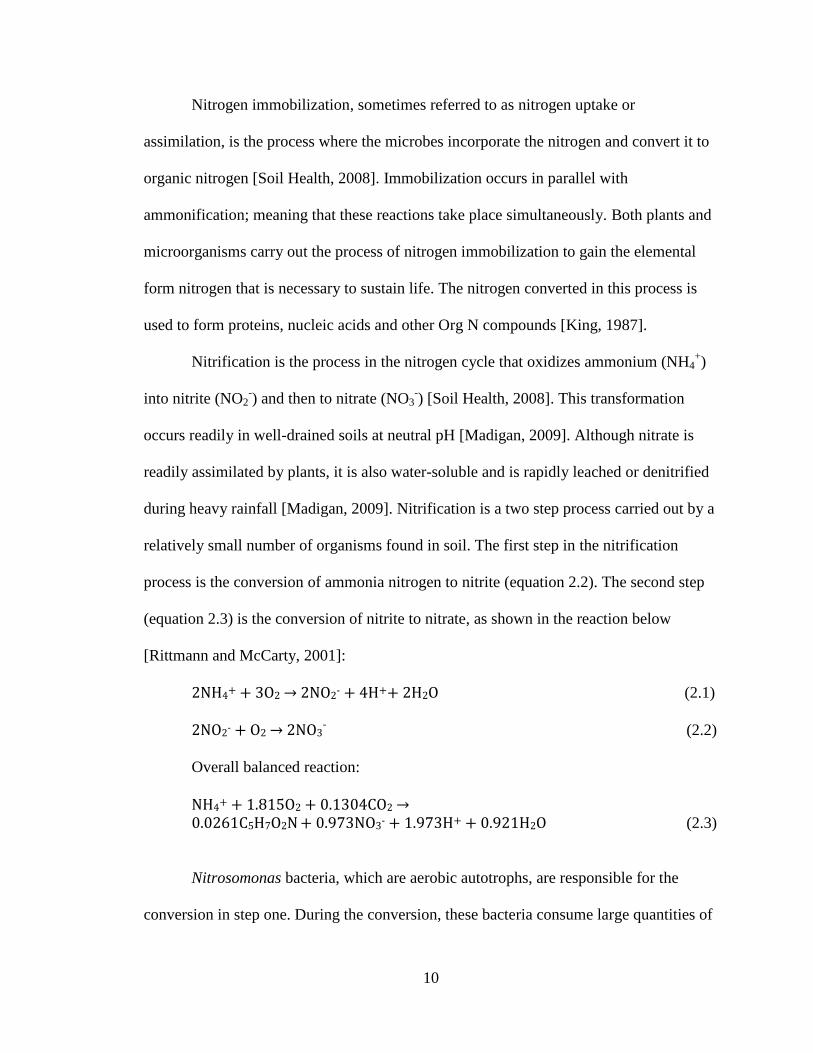
Nitrification is the process in the nitrogen cycle that oxidizes ammonium (NH4+)
into nitrite (NO2-) and then to nitrate (NO3
-) [Soil Health, 2008]. This transformation
occurs readily in well-drained soils at neutral pH [Madigan, 2009]. Although nitrate is
readily assimilated by plants, it is also water-soluble and is rapidly leached or denitrified
during heavy rainfall [Madigan, 2009]. Nitrification is a two step process carried out by a
relatively small number of organisms found in soil. The first step in the nitrification
process is the conversion of ammonia nitrogen to nitrite (equation 2.2). The second step
(equation 2.3) is the conversion of nitrite to nitrate, as shown in the reaction below
[Rittmann and McCarty, 2001]:
2NH4+ + 3O2 → 2NO2- + 4H++ 2H2O (2.1)
2NO2- + O2 → 2NO3- (2.2)
Overall balanced reaction:
NH4+ + 1.815O2 + 0.1304CO2 → 0.0261C5H7O2N + 0.973NO3- + 1.973H+ + 0.921H2O (2.3)
Nitrosomonas bacteria, which are aerobic autotrophs, are responsible for the
conversion in step one. During the conversion, these bacteria consume large quantities of
11
dissolved oxygen (DO), while reducing the alkalinity. Nitrobacter, which are also aerobic
autotrophs, are responsible for converting the nitrite to nitrate. Nitrobacter have a faster
growth rate than Nitrosomonas, therefore, once the ammonia is converted to nitrite, the
conversion to nitrate occurs rapidly.
Denitrification is the transformation pathway in the nitrogen cycle that completely
removes nitrogen the bioretention cell, with its end product being N2 [Harrison, 2003].
The nitrate reduction reaction includes intermediate steps in which nitrate is transformed
to nitrite, to nitric oxide, to nitrous oxide,and then to N2 [Metcalf and Eddy, 2003]:
NO3- NO2- NO N2O N2 (2.4)
A specialized group of bacteria are responsible for the process of denitrification.
These bacteria are known as denitrifiers (Rittman and McCarty, 2001). Denitrifiers are
facultative aerobes; which means that they have the ability to shift from aerobic to nitrate
respiration when oxygen becomes limited. The “denitrifying bacteria use the nitrate as an
electron acceptor to oxidize organic matter anaerobically” [Madigan, 2009]. In well
oxygenated sediments, the denitrification process will be limited. However, in the deeper
sediments towards the bottom of the bioretention cell, where oxygen levels are low, the
environmental conditions will be favorable for the denitrification process.
In order for nitrate to be reduced to nitrogen gas there must be an available
electron donor, or an inorganic electron donor such as sulfur or carbon. Equation 2.4
represents an example of a reaction using an organic carbon source (Sawyer et al., 2003).
Equation 2.5 represents the overall autotrophic denitrification reaction when elemental
sulfur (S0) is utilized as the electron donor (Bachelor and Lawrence, 1978).

12
C10H19O3N + 10 NO3- 5 N2 + 10 CO2 + 3 H2O + NH3 + 10 OH- (2.5)
1 S0 + 0.4 CO2 + NO3- + 0.76 H2O + 0.08 NH4+
0.08 C5H7O2N + 1.1 SO4-2 + 0.5 N2 + 0.781 H+ (2.6)
Hazards Associated with Excess Nitrogen in Stormwater Runoff
One major contributor to non-point source pollution is from storm water runoff.
The pollutants found in storm water runoff negatively impact drinking water supplies,
recreational fishing areas and wildlife [USEPA, 2010]. In the 1970‟s the USEPA initiated
the Pollution Act, also known as the Clean Water Act, which mandated that all water
bodies in the US be suitable for swimming and fishing purposes [CWA, 1972]. In 1998
the EPA assessed approximately 32% of US surface waters to address water quality
concerns. Of those assessed, 40% of US streams, lakes and estuaries were not meeting
EPA‟s water quality standards (WQS) to support recreational activities [USEPA, 2000].
The major pollutants found in these impaired water bodies were non-point source
pollutants. Storm water is an example of a non-point source pollutant. As heavy rain
washes down concrete infrastructure it picks up contaminants such as sediments,
nutrients, heavy metals, bacteria, oils and greases; flushing them into receiving water
ways. These contaminants are harmful to both humans and wildlife.
According to the St. Johns River Water Management District in Florida, nearly
80% of external nutrient loading is conveyed by runoff [SJWMD, 2006]. Agricultural
stormwater runoff plays a major role in the contamination of aquatic ecosystems across
the US, and in Florida. Nearly all of the estimated 242 million acres of land used to grow
crops in the US is maintained with pesticides and fertilizers [USDA, 2002]. Fertilizers
contain high concentrations of nitrogen and phosphorus (plant food). Pesticides contain

13
heavy metals such as arsenic, mercury and lead. Although the application of fertilizers
and pesticides may be essential to provide adequate food supplies to expanding
populations, in excess these harmful contaminants are being carried away by heavy rains;
and are ending up in our surface and groundwater.
Nitrogen and Phosphorus rich pesticides and fertilizers are frequently used in
urban areas as well. In fact many Americans use these products to fertilize their lawns.
Throughout Southwest Florida, annual plants, vegetables and lawns sometimes need
additional nutrients from fertilizer. When these nutrients are picked up by stormwater in
urban areas they accumulate, because the runoff is not able to undergo pre-development
hydrologic processes [OEC, 2010]. Figure 2.1 illustrates pre- vs. post-development
hydrologic flows. The figure shows that in urban areas there is an increase in surface
runoff, due to a decrease in porous surfaces. In large cities impervious infrastructure can
sprawl for miles. Therefore, it is not uncommon to find receiving water ways (e.g., rivers,
lakes and streams) impaired; due to a flux of harmful pollutants during storm events.
Figure 2.1. Pre-development vs. post-development hydrologic cycle [Maryland DEP,
2010].

14
Nutrients, such as nitrogen, can also be distributed to lakes and streams via
atmospheric deposition. The USEPA list three types of atmospheric deposition processes;
wet deposition, where pollutants are distributed through rain or snow; dry deposition,
where winds move particles through the air; and gas absorption, the dominant
atmospheric deposition process for many semivolatile persistent bioaccumulative toxic
pollutants [USEPA, 2010]. Lightning plays a role in nitrogen absorption process in the
atmosphere. “The enormous energy of lightning breaks nitrogen molecules and enables
their atoms to combine with oxygen in the air forming nitrogen oxides (NOx)” [Kimball,
2008]. These nitrogen oxides will then dissolve in precipitation, forming NO3- ions,
which are then transported to the soil during a storm [NPAP, 2010].
Nitrate ions are negatively charged (NO3-), and therefore they do not adhere well
to the soil particles (which are also negatively charged). Nitrogen can be very harmful to
the human health and aquatic ecosystems, as elevated levels of nitrate (NO3-) and/or
nitrite (NO2-) in drinking water can cause methemoglobinemia, or “Blue Baby
Syndrome” in infants. When infants ingest nitrate it can be reduced to nitrite in the body,
which can transform the oxygen binding hemoglobin into non-oxygen binding
methemoglobin [Fewtrell, 2004]. Because of this health concern, the United States
Environmental Protection Agency (USEPA) set a drinking water maximum contaminant
level (MCL) at 10 mg/L and 1 mg/L (as nitrogen) for NO3- and NO2
-, respectively
[USEPA, 2003].
The impact of nitrogen on human health is undeniable; what‟s more, increased
nitrogen and phosphorus in aquatic ecosystems can cause environmental degredation to
aquatic ecosystems as well. When nitogen in the form of ammonium (NH4+) enters an

15
aquatic ecosystem, the result can be an increase in aquatic organisms, which can decrease
dissolved oxygen (DO) levels in the water due to the oxygen demand when NH4+ is
converted to NO3- through the process of nitrification [Metcalf and Eddy, 2003]. The loss
of DO results in poor water quality conditions for aquatic life, and can leave an aquatic
ecosystem in despair.
In 2006, a local consulting firm, Janicki Environmental, published an analysis of
the impacts of Nitrogen loading on seagrass coverage in the Tampa Bay estuary. Seagrass
is beneficial to aquatic ecosystems, as it provides habitat to as many as 40,000 fish
species, and 50 million small invertebrates; and it filters suspended solids out of the water
column, improving water clarity [Hill, 2002]. However, seagrass (like many other plants)
cannot tolerate over-enrichment from concentrated runoff. In the 1970‟s, due to increased
urbanization and industrialization of the Tampa Bay area, the receiving water ways (the
Tampa Bay and its surrounding water bodies) saw an increase nitrogen and phosphorus
loading [Pribble et al., 2001, Poe et al., 2005].
After strict water quality criteria were mandated by the CWA for point-source
polluters, the Tampa Bay estuary began to see an increase in sea grass coverage.
However, due to non-point source pollution remaining untamed, today only 70% of the
seagrass has been restored in this region [Janicki and Greening, 2006]. State and local
regulations now aim to reduce the impact of nitrogen loading to the bay, by reducing non-
point sources of pollution from stormwater runoff [SWFWMD, 2010].
Stormwater Management: Low Impact Development Technologies
Approximately 80% of the US population lives in coastal communities and
Southwest Florida has experienced some of the nation‟s most rapid coastal development.

16
Dramatic landscape changes have occurred since the time of early settlement of
Southwest Florida - records show that the one square mile aggregate urban area of the
1890s grew to more than 80 square miles by the 1990s [SWFWMD, 2006]. During this
same period, vegetated uplands (e.g. forest, shrub, and brushland) decreased by 76%
[SWFWMD, 2006]. These changes have had a profound effect on the hydrologic cycle;
pervious spaces have been converted to land uses with increased impervious surfaces,
resulting in increased runoff volumes and pollutant loadings. Adding to the problems of
urban runoff is the fact that Southwest Florida is a karst region, where porous carbonate
rocks create a highly heterogenous aquifer system with rapid ground water movement
and recharge [USGS, 2001]. In karst regions, large volumes of stormwater rapidly
undermine the bedrock, thereby increasing groundwater pollution [USGS, 2001]. In
addition, the region is highly dependent on groundwater resources, with nearly 80% of
the 1 billion gallons of water used daily by residents coming from the Floridian aquifer
[SWFWMD, 2001].
A number of BMPs are used to control stormwater runoff, including structural
BMPs (previously listed) as well as non-structural BMPs such as education and
maintenance programs [Shoemaker et al. 2002]. Conventional stormwater ponds are
designed to minimize flooding by channeling runoff to a depressed area. Water then
either slowly infiltrates the underlying soil (retention pond) or is gradually released to an
adjacent surface water body (detention pond). Conventional stormwater ponds can be
designed to both control flooding and improve water quality [University of Wisconsin,
2005]; however, some studies have shown little improvement in nutrient loadings in these
systems [Mallin et al., 2000].

17
“Low impact development (LID) is an approach to land development (or re-
development) that works with nature to manage stormwater as close to its source as
possible. LID employs principles such as preserving and recreating natural landscape
features and minimizing impervious surfaces” [City of Poulsbo, 2009]. LID is
economically appealing to stormwater management professionals, as it is relatively
inexpensive to retrofit a current site. Additionally, LID provides aesthetic appeal to some
urbanized areas, which may have previously been a sore spot in the community.
LID is gaining popularity in urban cities as it emphasizes on-site treatment and
infiltration of stormwater, in contrast to “conventional stormwater controls, which collect
stormwater from impervious surfaces and transport the flow off site through buried pipes
to treatment facilities or directly to receiving” bodies of water [Econet, 2010]. The use of
LID practices is beneficial to the environment because it reduces disturbance of the
development area and the preservation of the pervious landscape. It can also be less cost
intensive than traditional stormwater control mechanisms [USEPA, 2000]. LID
techniques can be used in retrofitting existing urban areas with pollution controls, as well
as in new developments [Byrne, 2008]. The following are LID technologies that are
being used by stormwater management professionals to diminish non-point source
pollution from stormwater runoff:
Vegetated Rooftops
Permeable Pavement
Rain Barrels
Bioretention Cells/Bioswales (addressed in this research)

18
Vegetated rooftops, or green roofs, get their name from their design features;
they‟re constructed in multiple layers (Figure 2.2), consisting of a vegetated layer, media,
a geotextile layer and a synthetic drain layer [USEPA, 2000]. The most notable feature of
vegetated rooftops is the inclusion of the natural flora and soil/media components on top
of urban infrastructure. The vegetated rooftops are appreciated by many interest groups,
as they often provide a beautiful park or recreation area in sterile developed urban area.
“Even in densely populated areas, birds, bees, butterflies and other insects can be
attracted to green roofs and gardens up to 20 stories high” [The London Ecology Unit,
1993].
A green roof meets LID expectations, as they efficiently capture and temporarily
store urban stormwater runoff; which helps to maintain the pre-development peak
discharge rate. Generally runoff interception can vary from 15-90% based on soil depth,
and rainfall intensity [USEPA, 2000]. Figure 2.3 shows the ability of a vegetated rooftop
with a 3.35-inch soil thickness to reduce runoff during a 24 hour storm event [Roof
Scapes, Inc., 2000]. In addition to their ability to retain stormwater runoff, vegetated
roofs can also reduce the urban heat island effect by increasing evapotranspiration and
providing shade [Bass, 1999]. Although these urban retrofits are aesthetically pleasing,
this LID technology does not incorporate a media layer to achieve TN removal.

19
Figure 2.2. Depiction of the different layers found in a typical vegetated rooftop [USEPA,
2010].
Figure 2.3. Stormwater runoff from a 3.35-inch green roof, during a 24-hour rainfall
event [Roofscapes, Inc., 2000].
Permeable pavement is a LID technology that replaces non-pervious urban
roadways and sidewalks with pervious surfaces; where stormwater runoff can then
infiltrate more readily. A traditional, non-pervious urban pavement system contributes to
flooding and pollution issues associated with non-point source pollutant contamination.
Stormwater runoff permeates through the porous pavement into the underlying
Direct
Runoff Infrastructure
with Vegetated
Rooftop

20
gravel/stone layer. The underlying layer acts as a filter, cleaning out the pollutants
[USEPA, 2000]. There are a many urban areas utilizing this new technology, including
SWFL [Sarasota County, 2009]. However, overall construction costs must consider
maintenance issues, as the permeable surfaces are prone to clogging [USEPA, 2000].
There are several different types of pervious pavements, which include: (1) Plastic
pavers: A plastic honeycomb grid in which grass or other vegetation can grow; (2)
Concrete pavers: Concrete blocks with spacers in between them (for better drainage) and;
(3) Asphalt/concrete: Fine particles are left out, to improve porosity [Bean et al., 2004].
Rain barrels are an excellent LID technology, as they are easily installed and
relatively cheap; therefore making them affordable for private homeowners. Rain barrels
are large contains that attach to roof gutters (Figure 2.4). A traditional home is equipped
with rain gutters, which are designed to concentrate stormwater runoff to designate
outlets; therefore reducing the flooding around a residential home (for example). “A
typical 1/2-inch rainfall will fill a 50- to 55- gallon barrel” [SWFWMD, 2010]. “A 2,000-
square-foot roof can collect about 1,000 gallons of water per year (accounting for about a
20% loss from evaporation, runoff and splash)” [SWFWMD, 2010].

21
Figure 2.4. Typical rain barrel setup, to collect stormwater runoff from a rooftop [source:
http://www.ci.berkeley.ca.us]
Rainwater harvesting practices have been used to capture stormwater used for
drinking water since the Bronze Age (2000-1200 B.C.) [Hunt, 1999]. Today many
developing nations still collect rainwater for drinking water purposes. However, in the
developing country the improper treatment of rainwater would only be used for non-
potable (non-drinkable) water uses [Hunt, 1999]. Some common uses for the non-potable
rainwater collected in a rain barrel include: irrigating lawns and landscapes, flushing
toilets and washing vehicles [Hunt, 1999]. Often rain barrels are incorporated into a
larger LID system; where a vegetated roof will filter stormwater, which would collect in
a rain barrel, and then possibly into a bioretention cell. Because of its low cost, many
homeowners in SW Florida are utilizing these LID technologies to reduce irrigation
costs, and to maintain landscapes during seasonal droughts [CUES, 2006].
Detention systems have been utilized in urban areas for many years, to control
flooding from stormwater runoff [University of Wisconsin, 2005]. More recently, LID
has employed the use of a detention system that incorporates a defined media

22
configuration, to achieve enhanced nutrient reductions [USEPA, 1999]. The bioretention
system, or rain garden, is configured with vertical layers of media that are able to achieve
different steps in the nutrient removal process. Figure 2.5 illustrates the conventional
bioretention cell configuration used to treat stormwater runoff.
Figure 2.5. Typical bioretention system [Prince George‟s County DEP, 1993].
Bioretention cells are considered a LID because the stormwater runoff flows
through the six components, where the various mechanisms are able to restore pre-
development, hydrologic flows. However, the most notable feature of these systems is
their ability to significantly reduce nutrients like nitrogen and phosphorus, petroleum-
based pollutants, sediments, and organic matter. Prince George‟s County Department of
Environmental Resources (PGCDER) reported that both total suspended solids (TSS) and
organic matter were reduced by 90% when utilizing a bioretention cell [PGCDER, 1993].
Recent research by Davis et al. [2001] showed a significant reduction in heavy-metal

23
contaminants (>92% for lead, copper and zinc), as well as for TP (80% reduction) and
ammonia (60-80% reduction). However, Davis et al. [2001] only saw nitrite + nitrate-
nitrogen (NO3--N) reductions of around 24%.
In a conventional bioretention system, a ponding area attenuates peak flows, and
then water slowly infiltrates through vegetated soil, mulch and sand layers to the natural
groundwater. Figure 2.6 shows a cross-sectional depiction of a conventional bioretention
cell. The surface layer of a bioretention cell is generally planted with vegetation such as
flowering plants and shrubs, to provide an aesthetic, landscaped area. Treatment of
stormwater runoff is achieved through evapotranspiration, plant uptake, biodegradation,
filtration and adsorption [USEPA, 1999].
Figure 2.6. Schematic of a conventional bioretention cell [MDE, 2000].
An alternative bioretention system design was proposed by Kim et al. [2003],
which resulted in significant removal efficiencies for total nitrogen. In this system, runoff
gradually infiltrates through a sand layer, where nitrification occurs. The nitrified
stormwater is then conveyed through a submerged (anoxic) denitrification region, which
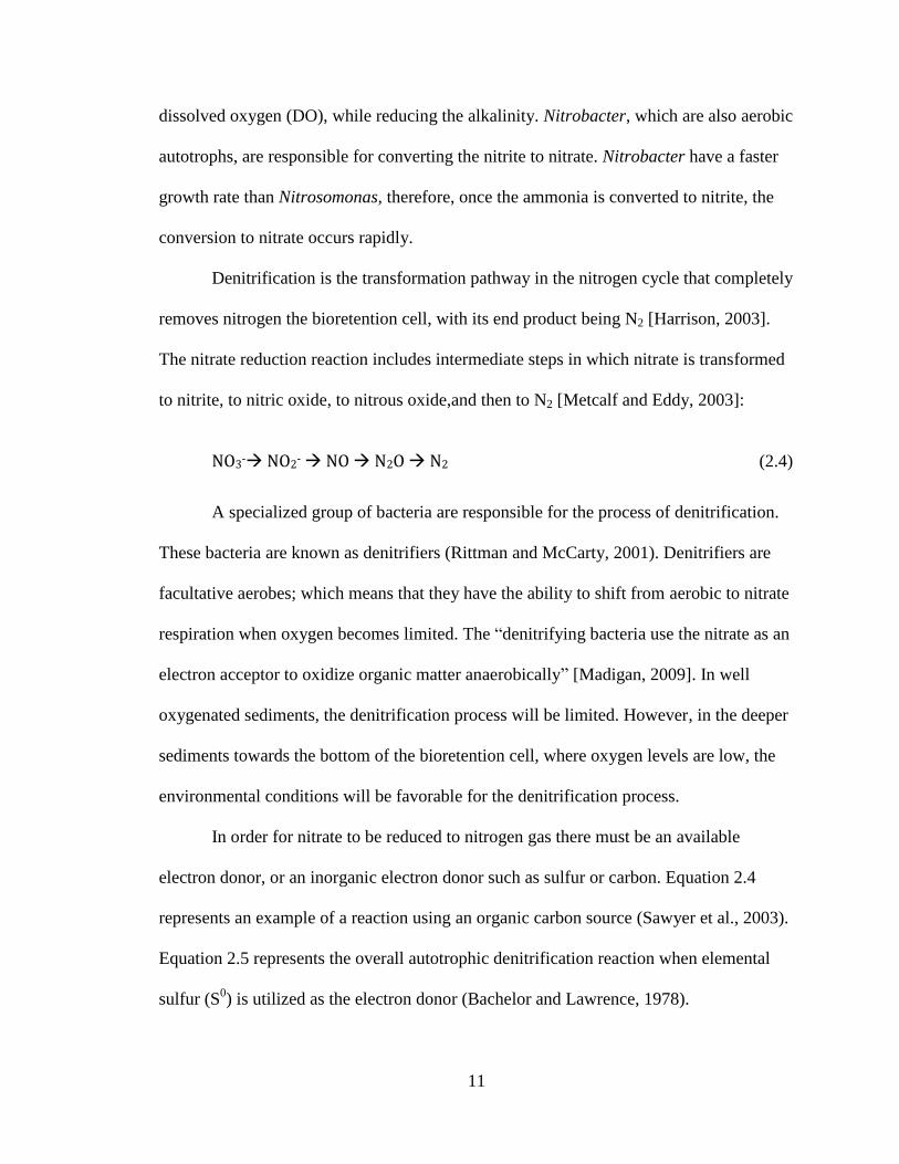
24
is supplied with an electron donor (e.g. wood chips as a carbon source), where nitrate is
reduced to nitrogen gas by anoxic heterotrophic bacteria. The outlet is configured so that
the denitrification zone remains submerged to maintain the anaerobic conditions required
by the denitrifying organisms. Figure 2.7 shows a cross-sectional illustration of an
alternative bioretention cell designed to achieve total nitrogen removal (the nitrification
occurs in aerobic sand layer and the denitrification in the submerged, anaerobic wood
chip layer) [adapted from Ergas et al. 2010].
Figure 2.7. Schematic of an alternative bioretention cell for treatment of nitrate rich
stormwater [Ergas et al. 2010].
Recently, Ergas et al. [2010] published results from a pilot-scale study using the
aforementioned nitrogen-removing bioretention system design. This study investigated
treatment of typical urban stormwater under controlled laboratory conditions followed by
two years of field studies with agricultural runoff. Results from this study showed high
total nitrogen removal efficiencies (>80%) when using wood chips as the denitrifying

25
media source. Additionally, this design achieved good overall average removal
efficiencies for COD (55%), BOD5 (69%), suspended solids (81%), total P (54%), and
PO43-
(48%) [Ergas et al., 2010].
The results of prior studies have shown that the use of this alternative bioretention
cell design can increase nitrogen removal, when compared to a typical bioretention cell
configuration. The incorporation of wood chips into bioretention media is effective in
removing nutrients from stormwater runoff. No controlled studies have been done
comparing the different designs and media materials under field conditions in SW
Florida, however. This is particularly important in Southwest Florida due to high rainfall
and water table level variations in the region. In addition, little data are available on the
maintenance requirements and long-term performance of these systems.
Environmental Considerations for Implementing LID in SWFL
To better understand the ability to effectively introduce bioretention cells to treat
stormwater runoff in SWFL it is first necessary to understand the dynamics of the local
hydrologic system. One main purpose for incorporating bioretention cells in SWFL is to
achieve groundwater recharge; therefore, it is necessary to thoroughly understand the
factors that influence the interaction between surface and groundwater, in the watershed
[Kish et al. 2007]. The purpose of this section will be to discuss the regional climate,
including the rainfall characteristics in Sarasota County. This section will then address
the geographic characteristics of Sarasota County; including the hydrogeology, the
watershed characteristics and the water use within Sarasota County.
A watershed is an area of land where all the groundwater and surface water drains
into the same water body [USEPA, 2009]. Sarasota County consists of six major

26
watersheds- Sarasota Bay, Little Sarasota Bay, Myakka River, Dona/Roberts Bay,
Roberts Bay and Lemon Bay- this project will focus specifically on the Lemon Bay
watershed (Figure 2.8). In July, 1986 the Florida Legislature designated Lemon Bay as an
aquatic preserve [Florida DEP, 2011]. At least 230 species of fish depend directly on the
mangroves and aquatic ecosystem of Lemon Bay. Lemon Bay is also home to endangered
species, like the manatee and sea turtle, which come to feed on the nearshore seagrasses
[Florida DEP, 2011]. The Lemon Bay watershed contains a series of creeks; this project
will focus specifically on the creek known as Alligator Creek, which can be seen in detail
in Figure 2.8. Alligator Creek is approximately four miles long, and drains into the
northern tip of Lemon Bay [Sarasota County Wateratlas, 2010].
A hydrologic cycle is a complex system that links climate, geography, soils,
hydrogeology, land cover, land use, and urbanization of a certain area, or watershed
[Kish et al. 2007]. The specific hydrologic system for the Lemon Bay watershed is linked
to the unique environmental setting of the area. According to Sarasota County‟s LID
Manual, LID technologies should be designed to mimic the natural hydrologic flows of a
proposed site [Sarasota County, 2009].
Southwest Florida is well known for its long, warm, humid summers and short,
mild, dry winters; these characteristics follow a somewhat predictable seasonal pattern
[Kish et al. 2007]. Typically, in the winter months (December through February) the
average temperature ranges from forty-eight degrees Fahrenheit in the evening hours, and
reach up to seventy-one degrees Fahrenheit in the day time; the summer months (June-
August) will typically see temperatures ranging from seventy-two degrees Fahrenheit to
ninety-one degrees Fahrenheit [Soil Conservation Service, 1991].

27
Figure 2.8. Detailed map of Alligator Creek, located within the Lemon Bay watershed
[Sarasota County Wateratlas, 2010].
Seasonal variations are seen in rainfall patterns in SWFL as well, but precipitation
events will often occur in somewhat predictable patterns; winter storms are mostly
formed by cold fronts moving south across the northern US, whereas tropical storms will
generally move northward across Florida, from the Atlantic, and local thunderstorms will
develop almost daily in the summer months [Kish et al., 2007]. Although these storms
seem somewhat predictable, the actual precipitation that any one storm event will
Alligator
Creek
Sarasota County Watershed
Map

28
produce, locally, varies substantially. Historical rainfall trends for Sarasota County show
that rain events will occur almost daily in the rainy period, from July through October;
however, in the dry period (November through June) rain events are sparse [SWFWMD,
2005].
The purpose of using an LID technology is to achieve predevelopment hydrologic
functioning of a site; therefore it is essential that this paper address the hydrogeology of
this region, in order to better understand the potential to implement this technology across
SWFL. This region is well known for its sandy soils. Florida was once at the bottom of
the ocean; therefore leading to topography consisting of a series of relict marine terraces
[Campbell, 1985]. Specifically, five hydrologic soil groups exist within Sarasota County,
as defined by the National Resource Conservation Service (NRCS): (1) Types A (well-
drained), B/D (moderately well-drained when dry, somewhat poorly drained when wet),
C (somewhat poorly drained), C/D (somewhat poorly drained when dry, poorly drained
when wet), and D (poorly drained) [Sarasota County, 2009]. Most soils are classified in
the B/D hydrologic soil group, due to a high water table [Sarasota County, 2009];
therefore, making them poorly drained and consisting of mucky, sandy or loamy soils
[Kish et al., 2007].
Soil characteristics play an important role in the hydrology of a watershed. Poorly
drained soils will lead to an increase in stormwater runoff, nutrient transport, and in
increase in depressional storage of water into nearby retention basins [Soil Conservation
Service, 1991]. According to the US Geological Survey‟s Websoil Survey, the proposed
site for the bioretention retrofit project consists of mostly Myakka fine sands (specifics of
this particular site and soil composition will be discussed in more detail in Chapter four

29
of this paper), which is classified as type B/D (moderately to poorly drained) soil.
Therefore, according to NRCS, during the wet weather season when the soil is saturated,
there will be in increase in stormwater runoff entering retention basins; however, in the
dry weather season, stormwater would percolate more readily into underlying
groundwater reservoirs. The hydrologic path taken by the stormwater would depend on
the precipitation duration and the depth to the underlying groundwater [Kish et al., 2007].
Groundwater is one of Florida‟s most valuable resources, as nearly 80% of the 1
billion gallons of water used daily by residents comes from the Upper Floridian Aquifer
[SWFWMD, 2001]. An aquifer is the term used to describe the location of the
groundwater. The three aquifers underlying Sarasota County, in ascending order, are the
Upper Floridian Aquifer, the intermediate aquifer system and the surficial aquifer system
[Barr, 1996]. The average depth to the surficial aquifer system in this region is generally
less than five feet (1.5 m) [Kish et al., 2007]. The depth to the surficial aquifer can vary
seasonally by as much as five feet (1.5 m) [Kist et al., 2007]; therefore, infiltration-
dependent LID-technologies will be constrained under wet weather conditions in this area
[Sarasota County, 2009].
Implementation of LID Technologies in Southwest Florida
The implementation of LID technology in Florida has been slow moving; as little
research is available to justify the effectiveness of these BMPs in SWFL. As previously
discussed, SWFL has very different hydrologic and geologic characteristics when
compared with the northwestern US; where successful implementation of LID
technologies originated. However, some LID projects were recently completed in
Sarasota, Dunedin and Hillsborough Counties. Table 2.2 provides an overview of
30
different types of LID projects that have recently been completed in southwest Florida, as
well as some background information for each project.
Of the six LID projects recently finished in SW Florida, only the Florida
Aquarium performed post-development nutrient analyses in order to justify the benefit of
utilizing LID in SW Florida. The USEPA [2000] released a literature review, which
summarized the results of the yearlong study conducted at the Florida Aquarium, from
1998-1999. The project was designed in an effort to detain all stormwater runoff onsite,
instead of allowing it to flood streets or flow into sewer systems and out into the Tampa
Bay. The entire 4.65 ha parking lot was used in this study to define the drainage basin
[USEPA, 2000]. Each parking space within the entire parking lot was shortened, to allow
enough space to retrofit a grassed swale between each row. Figure 2.9 shows a diagram
of the Florida Aquarium parking lot that was retrofitted with the bioretention cells and
permeable pavement in this project.
The study area for this project consisted of four separate scenarios, with a total of
eight basins (two basins for each of the four scenarios), and each configuration was
equipped with the appropriate analytical tools for collecting and monitoring stormwater
runoff. The first scenario was asphalt paving with no swale; the second included a swale;
the third scenario was traditional cement paving with a swale and; the final scenario
looked at permeable pavement with a connected swale. The results of this study highlight
that the poorest performance was seen with the asphalt with swale scenario [USEPA,
2000].

31
Table 2.1. Summary of LID projects in southwest Florida.
Type(s) of LID
Technology
Project
Name
Project
Location
Project Overview
Pervious
Pavement &
Grassed Swales
The Florida
Aquarium
Hillsborough
County
Permeable pavement laid for
parking lot of facility, with
stormwater runoff being
piped underground to grassed
swales
Detention with
Biofiltration
Clark
Station
Sarasota
County
Bioretention pond added to
existing BMP‟s for enhanced
nutrient reduction
Permeable Pavers Reid Habitat
for
Humanity
Sarasota
County
Limit fill required to grade
pre-developed land, and use
permeable pavers designed to
achieve 85% load reductions
Stormwater
Harvesting
The Bridges Sarasota
County
Use of existing ponds for
stormwater harvesting and
irrigation purposes
Cistern/Large
Rain Barrel &
Green Roof
South Lido
Beach Park
Restroom
Pavilion
Sarasota
County
Cistern provides non-potable
water for toilet flushing and
green roof proposed to
achieve a 75% load &
nutrient reduction
Pervious
Pavement
Dunedin
Community
Center
Pinehurst
Rd.
Dunedin, FL
Grassed parking lot;
reinforced with “Geo-Web”
Figure 2.9. Florida Aquarium project depiction [Rushton, 1999].

32
Modeling an Alternative Bioretention System
Although some studies have modeled the hydraulic performance of bioretention
systems [Lucas, 2010; Heasom et al., 2006; Abi Aad et al., 2010], presently there are no
studies that have modeled the efficiency of these alternative bioretention systems to
achieve denitrification. Considering that denitrifying bioretention systems are a relatively
new advancement in bioretention system design, it was not surprising that there is not
more literature on the ability to model nitrogen reductions in these systems. EPA‟s
SWMM-5 is capable of modeling low impact development technologies, yet it is not
capable of modeling an alternative (denitrifying) bioretention system. Therefore, a more
in-depth design was needed, in order to illustrate a multi-layered, alternative bioretention
system.
A case study analysis was performed, in order to determine the estimated nitrate
reductions of the proposed redesigned bioretention cells at the Venice, FL site using
SWMM-5 to simulate post-development annual nitrogen loading rates. The research for
this project was carried out in a four phase research process. The objective of Phase I was
to define site-specific input parameters of the proposed case study site where Sarasota
County will develop a series of bioretention cells in Venice, FL. The objective of Phase II
was to estimate the rate loss coefficient values (k1 and k2) for nitrification and
denitrification. The objectives of Phases III and IV of this project were to develop a
SWMM-5 model of an alternative (denitrifying) bioretention system, to evaluate the
hydrologic performance and estimate nitrogen removal efficiencies.
33
State and Local Regulations
The proposed site for the bioretention cell retrofit project discussed in the paper is
located in the city of Venice; which is in Sarasota County, FL. Sarasota County‟s Land
Development Regulations, Article I Sec. 74-4, requires development projects to provide
“adequate stormwater management [so as] to reduce the impact of flooding to a
minimum” and “protection of Sarasota County‟s natural systems and scenic resources,
including the quality of air and both surface and groundwaters and the preservation of
their ecological integrity” [Sarasota County, 2009]. LID is an effective tool which can be
used to reduce flooding and non-point source pollution, while meeting these County land-
development standards [Sarasota County, 2009].
Chapter 62-40.432 of the Florida Administrative Code (F.A.C.) defines the water
quality regulations in the State of Florida. Based upon the language outlined in this
chapter, all stormwater management systems designed within the State of Florida must
“achieve at least 80% reduction of the annual average load of pollutants that would cause
or contribute to violations of state water quality standards” (per Chapter 62-40.432
F.A.C.). New stormwater best management practices must address these regulations, and
be designed according to the guidelines established by this rule; then, presumably
discharge from these stormwater systems will meet state regulatory standards [Harper
and Baker, 2007]. According to SWFWMD, post-development nutrient characteristics
must meet, or be better than the pre-development characteristics. In order for a
stormwater development project to qualify for a NPDES permit, planners and/or
engineers must provide justified evidence that the post-development nutrient
characteristics will meet the State‟s rule requirements [SWFWMD, 2010].
34
Chapter Three:
SWMM-5 Capabilities
This chapter will discuss the purpose for incorporating the SWMM-5 model, the
SWMM-5 model framework and model inputs based on site -specific parameters, and
how the software quantifies hydrologic flows and total nitrogen removal.
SWMM-5 Software
The first Storm Water Management Model (SWMM) software was developed in
the early 1970‟s, and has undergone various transformations since its creation [USEPA,
2010]. The SWMM software can simulate a single precipitation event or provide long-
term simulations of water quality and quantity for a user defined drainage basin [USEPA,
2010]. The original SWMM software was not capable of addressing methods for layered
biofiltration systems [Lucas, 2010]. The latest version of the SWMM software, (SWMM
5.0.021) “operates on a collection of subcatchment areas (and now LID/BMP areas) that
receive precipitation and generate runoff and pollutant loads after simulation evaporation
and infiltration losses from the drainage basin” [USEPA, 2010]. This section will
compare different approaches to simulating nutrient treatment, compare the capabilities
of the latest SWMM software, and provide details on the various components of SWMM-
5 and their uses.
The EPA SWMM-5 software is free, downloadable software provided by the
USEPA (at http://www.epa.gov/ednnrmr/models/swmm/index.html). The benefit of using

35
the SWMM-5 software for this project is its ability to compare the pre- vs. post-
development hydrologic model outputs. Comparing the pre- vs. post-development results
allows engineers and planners to make better decisions about the hydrologic impact on
planned development areas [Jang et al., 2007].
SWMM-5 was designed to account for the various hydrologic processes that can
differ at each site, including; “time-varying rainfall, rainfall interception from depression
storage, infiltration of rainfall into unsaturated soils, percolation of rainwater into
groundwater layers, interflow between groundwater and the drainage system, nonlinear
reservoir routing of overland flow and runoff reduction via LID components” [USEPA,
2010]. The subcatchment properties for a bioretention cell in the SWMM-5 model are
listed in Table 3.1.
Table 3.1. General subcatchment characteristics as defined in SWMM-5 [adapted from
Abi Aad et al. 2010].
Subcatchment
Properties
Area
Input Values
Area of the subcatchment; it depends on the availability of land on
the parcel
Width Characteristic width of flow running over the subcatchment
Slope Percent slope of the water surface flowing over the subcatchment
Imperviousness Percent of impervious area
Impervious N Manning‟s factor n for the impervious portion of the subcatchment
Pervious N Manning‟s factor n for the pervious portion of the subcatchment
Dstore-imperv Depth of depression storage on the impervious area (in.)
Dstore-perv Storage depression over the pervious portion of the subcatchment
% zero-imperv Percent of the impervious area with no depression storage
Outlet Defines the node receiving the flow

36
SWMM-5 Compartments
“There are four major categories to conceptualize a drainage system as water and
material flows between environmental compartments that the SWMM5 model addresses:
the atmospheric compartment, the land surface compartment, the groundwater
compartment and the transport compartment” [USEPA, 2010]. Not all compartments
must be considered for every model [USEPA, 2010]. The atmospheric compartment
addresses rainwater and nutrient inputs, which is represented as a rain gauge. The land
surface compartment (subcatchment) addresses the pervious receiving area and the
outflow leaving this area. One or more subcatchments can be used to represent different
drainage areas. There is also a groundwater compartment, which was not used to develop
the model in this study. The transport compartment includes orifices. Orifices were used
to control flow into the storage unit nodes in the model developed for this case study.
More details about the different compartments used to develop the model in this study are
listed in the following subsections.
Atmospheric Compartment
Rain gauges are used to supply one or more subcatchments with precipitation
data. Multiple rain gauges can be incorporated into a SWMM-5 model, in order to
evaluate single-event storms. The rain gauge used for this model is a user-defined time
series. Specific details regarding the rainwater data are presented in Chapter 6.
Land/Subcatchment Compartment
Subcatchments in the SWMM-5 model represent the hydrologic flow of
stormwater runoff across a defined drainage area. A single subcatchment was used to
represent the drainage basin; draining into the thirteen bioretention cells along Venice

37
East Blvd., for this case study. The breakdown of nitrogen is represented using a system
of nodes (a node is defined in more detail below).
A subcatchment can drain into another subcatchment, or into a defined node.
There are four different types of nodes that can be used to model drainage systems in
SWMM5: junctions, outfalls, dividers and storage units. A storage unit node was used
for this model; reasons for choosing to use a storage unit node will be discussed in the
following subsection. As previously discussed, a subcatchment can be subdivided into
permeable and impermeable subareas. “Impermeable subareas within a subcatchment can
be further divided into two subareas- one with depression storage and/or one without”
[USEPA, 2010]. The stormwater runoff from the impervious drainage area was routed to
drain to a storage unit node for the model developed in this study.
Storage Unit
A storage unit node was selected for the development of the model in this study,
to represent the different layers within a bioretention cell. The storage unit node is a good
object to use for this study, because it allows for treatment within each node. Therefore,
each layer can account for a different process within the alternative bioretention cell by
inputting treatment expression specific to the nitrification and denitrification processes
(treatment expressions are discussed in detail in the subsequent section). The principle
input parameters for the storage nodes used for this project are shown in Table 3.2.

38
Table 3.2. Principle input parameters needed to calibrate the SWMM-5 model for this
case study. [Adapted from USEPA, 2010]
Storage Unit Node: Input Parameters
Invert Elevation
Maximum Depth
Ponded Area
Treatment
Infiltration
Storage Curve
Computational Capabilities
“The precipitation flowing to the permeable subarea of a subcatchment into the
unsaturated upper soil layer can be incorporated into simulations run in SWMM-5 using
three different methods: the Horton infiltration method, the Green-Ampt method and the
Curve Number infiltration method” [USEPA, 2010]. The variations between each
infiltration method and the method that was selected for the model designed in this study
are described below.
Horton Infiltration Method
Horton‟s Equation is used to describe groundwater infiltration rates or volumes
[Dickenson, 2008]. The equation “represents an empirical formula, where the rate at
which water percolates through the soil surface is constant and then begins to decrease
over time” [Dickenson, 2008]. The percolation rate eventually levels off when the soil
saturation level reaches a fixed value. Horton‟s equation can also be used to calculate the
total volume of infiltration after a period of time. The input SWMM-5 parameters for this
method include the “maximum and minimum infiltration rates, a decay coefficient which
describes how fast the rate decreases over time, and the time it takes a fully saturated soil
to dry” [USEPA, 2010].

39
Curve Number Infiltration Method
The curve number method (CN method), also termed the runoff curve number
(RCN), is an empirical formula developed by the USDA. The CN method is used in
hydrologic calculations to determine the amount of runoff or direct infiltration of runoff
from a storm event [USDA, 1986]. The runoff curve number is based on hydrology, soil
conditions, land use and treatment. “The input parameters for this method are the CN and
the time it takes a fully saturated soil to dry completely” [USEPA, 2010].
Green-Ampt Infiltration Method
In this work, the Green-Ampt method [Green and Ampt, 1911] was selected for
modeling infiltration. The Green-Ampt equation is a “semi-theoretical formula”, which
was used most often, in comparable studies, when modeling bioretention cells [Lucas,
2010; Tsihrintzis and Hamid, 1998; Abi Aad et al., 2010]; as the Green-Ampt method is
“well suited for predicting surface runoff from the pervious” area of a bioretention cell
during a storm event [Heasom et al., 2010]. Before a storm event the soil moisture
content is assumed to be able to sufficiently able to handle infiltration. During a storm
event the stormwater will flow through the spaces between the soil particles, creating a
wetting front. “Gravity, the matrix potential of the dryer soil underneath, and Darcy‟s
Law are all important factors in the downward flow of the stormwater into the underlying
soil layer” [Heasom et al., 2010].
Modeling Treatment with SWMM-5
The SWMM5 software is also capable of predicting the reduction of pollutants
through treatment in storage units, by analyzing the buildup, washoff, transport and
treatment of any number of constituents. The ability to model the removal of pollutants

40
was the key factor in selecting the SWMM5 model for this research. Within the model,
removal of pollutants can be dependent on co-pollutants. For example, in the model
developed in this project NO3- was considered a co-pollutant, as the concentration
following into the denitrification layer was dependent on the concentration of the reacted
NH4+
exiting the nitrification layer. “Treatment can be modeled by using treatment
functions within a node, and mathematical expressions for computational purposes”
[USEPA, 2010]. For purposes related to the model developed for this research, the
pollutant removal was expressed as a concentration (C). The equations derived for the
SWMM-5 model developed in this project are presented in Chapter 5.
LID Components
SWMM-5 is capable of modeling LID, including: bioretention cells, infiltration
trenches, porous pavement, rain barrels and vegetative swales [USEPA, 2010]. This
project was specifically interested in the capability of SWMM-5 to model the efficiency
to achieve denitrification in an alternative (denitrifying) bioretention system. “Because
the LID controls cannot act in series”, SWMM5 is not capable of modeling the capability
of LID controls to achieve denitrification [USEPA, 2010]. Therefore, the model designed
for this project quantifies treatment within a bioretention system by using a network of
storage units (where each storage unit represents a different treatment layer in an
alternative bioretention cell); each with its own treatment capabilities. More details on the
conceptual framework, including a diagram of how runoff flows through the system, can
be seen in Chapter 6.

41
Chapter Four:
Site Characteristics
The overall goal of this research project was to investigate the performance of a
proposed bioretention system in Venice, FL to treat non-point sources of nitrogen from
stormwater runoff. Phase I of this project was to determine the hydrologic and quality
characteristics of the pre- developed bioretention retrofit site in Venice, FL. This chapter
includes a description of the site, including runoff and physical characteristics based on
the literature, as well as information on the proposed bioretention system. Site-specific
nutrient characteristics analyzed during Phase I of this project are discussed in Chapter 5.
Physical Characteristics
The site for the proposed bioretention cell retrofit project (Figure 4.1) is located
on Venice East Blvd. in the City of Venice, FL. This area is coded as a single-family
residential community, as defined by the Florida Land Use Code and Classification
System. The four-laned road is curbed, with storm sewers that drain into a retention basin
that runs perpendicular to Venice East Blvd. This retention basin empties out into
Alligator Creek, and then into Lemon Bay. The purpose of the retrofit project is to
significantly reduce the nutrient loading to Alligator Creek, an impaired water body, by
reducing the nitrogen concentration in the stormwater runoff. This will be achieved by
increasing the pervious area to allow an increase in groundwater infiltration. The
proposed project includes cutting the curbed gutter at specified locations, to allow some
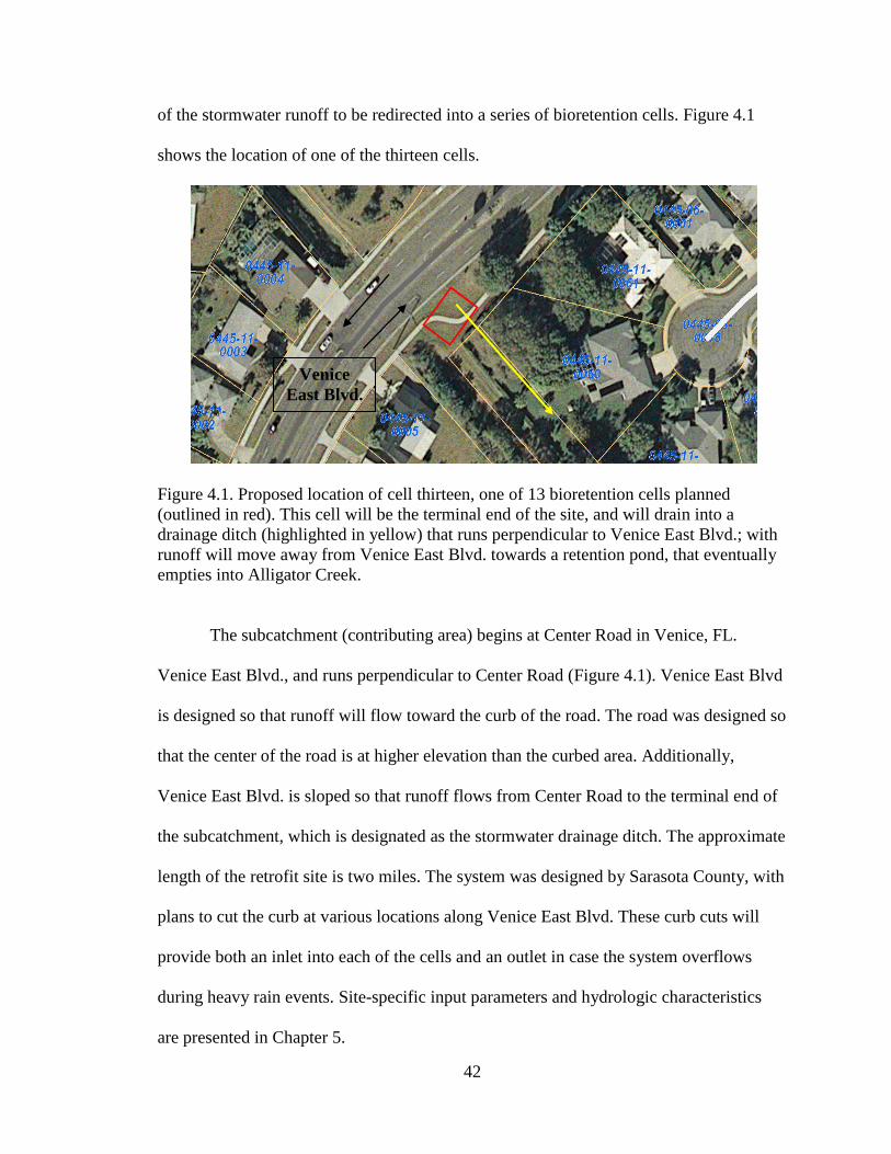
42
of the stormwater runoff to be redirected into a series of bioretention cells. Figure 4.1
shows the location of one of the thirteen cells.
Figure 4.1. Proposed location of cell thirteen, one of 13 bioretention cells planned
(outlined in red). This cell will be the terminal end of the site, and will drain into a
drainage ditch (highlighted in yellow) that runs perpendicular to Venice East Blvd.; with
runoff will move away from Venice East Blvd. towards a retention pond, that eventually
empties into Alligator Creek.
The subcatchment (contributing area) begins at Center Road in Venice, FL.
Venice East Blvd., and runs perpendicular to Center Road (Figure 4.1). Venice East Blvd
is designed so that runoff will flow toward the curb of the road. The road was designed so
that the center of the road is at higher elevation than the curbed area. Additionally,
Venice East Blvd. is sloped so that runoff flows from Center Road to the terminal end of
the subcatchment, which is designated as the stormwater drainage ditch. The approximate
length of the retrofit site is two miles. The system was designed by Sarasota County, with
plans to cut the curb at various locations along Venice East Blvd. These curb cuts will
provide both an inlet into each of the cells and an outlet in case the system overflows
during heavy rain events. Site-specific input parameters and hydrologic characteristics
are presented in Chapter 5.
Venice
East Blvd.

43
Proposed Bioretention System Design
The system of thirteen cells was designed by Sarasota County with no
connections between each of the thirteen cells. Each cell is designed as a closed system
(i.e., effluent from one cell will not influence flows or nitrogen loads into the next cell).
The system of cells is designed so that all impervious flows will be routed toward the
bioretention cells. The impervious area at the Venice East Blvd. bioretention site
accounts for approximately 41.8 % of the total area.
Sarasota County provided plans for cell number 13; one of thirteen proposed cells
at the Venice East Blvd. site. All 13 cells were assumed to be of equal size. Cell 13 is
approximately 23.4 m long by 9.14 m wide (76.7 ft by 30.0 ft). Therefore, the total area
for all thirteen cells is approximately 2,780 m2 (29,900 ft
2). The media begins
approximately 86.4 cm (34 inches) below the existing grade, with the top of the media at
approximately 55.9 cm (22 inches) below the lip of the bioretention cell.
Figure 4.2. Site plan of bioretention cell 13 [plans provided by Sarasota County].
6-inch Mulch/Denitrification
Layer
12-inch Sand/Nitrification
Layer
3-inch Mulch Layer
4-inch Soil/Vegetation
Layer
Ponding Level < 12”
Filter Fabric Envelope

44
Runoff Characteristics
Table 4.1 presents typical constituents analyzed in stormwater runoff, the
analytical methods used, the method detection limits for each constituent, and the typical
concentration of each constituent in stormwater runoff in Florida based on the literature.
Many of these same constituents were analyzed during Phase I of the model
development, as discussed in Chapter 5.

45
Table 4.1. Analytical methods summary and typical nutrient concentrations.
Analyte Analytical Method
Method
Detection
Limit
Typical Conc. in
Stormwater Runoff
based on Literature
Total Nitrogen (TN) HACH Test „N Tube:
Persulfate Digestion Method 0.5 mg/L as N
1.17 mg/L [for a grassed
swale in Sarasota County
ERD (2004)]
Ammonium (NH4+-N)
APHA et al. Standard
Method
4500-NH3 D
0.06 mg/L as
N
0.17 mg/L [Dillon &
Chanton, 2005]
Total Kjeldahl
Nitrogen (TKN)
APHA et al. Standard
Method 351.2 0.594 mg/L
1.55 mg/L
[PBS&J, 2010]
Ammonia (NH3-N)
APHA et al. Standard
Method 4500-NH3 C 0.005 mg/L 0.31 mg/L [PBS&J, 2010]
Nitrate + Nitrite as
Nitrogen
APHA et al. Standard
Method 353.2
0.005 mg/L as
N
0.42 mg/L [(nitrate-nitrite
combined) PBS&J, 2010]
Org N Calculated by Difference* N/A 1.38 [PBS&J, 2010]
Ortho-Phosphorus as P APHA et al. Standard
Method 365.3 0.002 mg/L 0.34 mg/L [PBS&J, 2010]
Total Phosphorus (TP)
HACH Test „N Tube: APHA
et al. (2005) SM4500-P E
0.02 mg/L as P
0.506 mg/L [for a grassed
swale in Sarasota County
ERD (2004)]
5-day
Biochemical Oxygen
Demand (BOD5)
APHA et al. (2005) Standard
Method 5210B: 5-Day BOD
Test
0.5 mg/L
4.4 mg/L [for a grassed
swale in Sarasota County
ERD (2004)]
Alkalinity
APHA et al. (2005) Standard
Method 2320B: Titration
Method
0.67 mg/L as
CaCO3
20.91 mg/L [(North
Florida stormwater) H.
Zhang, 2010]
Total Suspended
Solids (TSS)
APHA et al. (2005) Standard
Method 2540D 0.57 mg/L
10.1 mg/L [for grassed
swale in Sarasota County
ERD (2004)]
Volatile Suspended
Solids (VSS)
APHA et al. (2005) Standard
Method 2540E 0.57 mg/L N/A
Total Coliform Units
(CFU)
APHA et al. (2005) 9222B:
Membrane Filtration Test
20 CFUs per
plate required
to assume
validity
N/A
Dissolved Oxygen
(DO)
APHA et al. (2005) Standard
Method 4500H 1.01 mg/L N/A
pH APHA et al. (2005) Standard
Method 4500H 0-14 pH units
7.78 [(N. Florida
stormwater) H. Zhang,
2010]
*Org N was calculated by the difference between the TKN and NH4+ concentrations

46
Chapter Five:
Methods
The project was carried out in four phases. Each of the four phases, including the
purpose for each phase, is defined in Table 5.1. This Chapter will discuss each phase in
detail, and will define the conceptual model framework for an alternative bioretention
system.
Table 5.1. Four phases to develop the alternative bioretention cell model and the purpose
for each phase
Phase Description Purpose
Phase I Site-Specific Nutrient
Characterization
Nitrogen concentrations needed for
SWMM-5 pollutant input parameters
Phase
II
Analytical Bioretention System
Model
Data from Siegel (2009) were used
to estimate first-order rate
coefficients for nitrification and
denitrification
Phase
III
SWMM-5 Hydrologic ABC Model Site-specific input parameters from
the literature were used to develop a
ABC model
Phase
IV
SWMM-5 Water Quality ABC
Model
Treatment expressions were derived
in order to estimate nitrogen
reductions
Phase I: Site-Specific Nutrient Characterization
In order to define site-specific nitrogen input parameters for the SWMM-5 model
designed in this project, it was necessary to characterize the concentrations of nutrients at
the proposed bioretention retrofit site. The parameters I analyzed during Phase I were
selected because they are typically analyzed in stormwater runoff, as discussed in
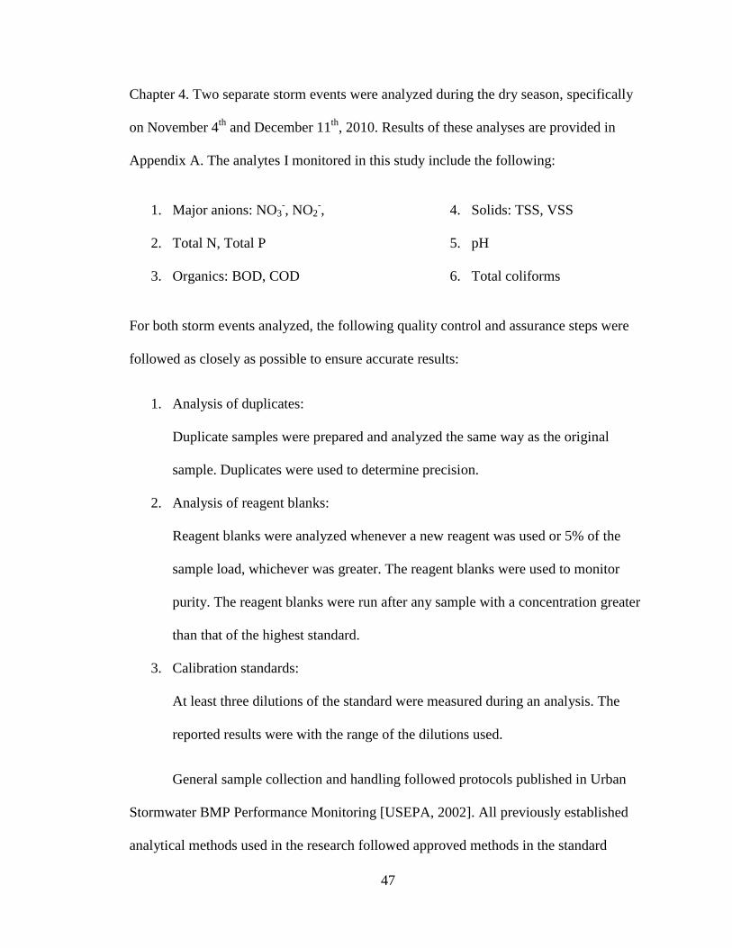
47
Chapter 4. Two separate storm events were analyzed during the dry season, specifically
on November 4th
and December 11th
, 2010. Results of these analyses are provided in
Appendix A. The analytes I monitored in this study include the following:
1. Major anions: NO3-, NO2
-,
2. Total N, Total P
3. Organics: BOD, COD
4. Solids: TSS, VSS
5. pH
6. Total coliforms
For both storm events analyzed, the following quality control and assurance steps were
followed as closely as possible to ensure accurate results:
1. Analysis of duplicates:
Duplicate samples were prepared and analyzed the same way as the original
sample. Duplicates were used to determine precision.
2. Analysis of reagent blanks:
Reagent blanks were analyzed whenever a new reagent was used or 5% of the
sample load, whichever was greater. The reagent blanks were used to monitor
purity. The reagent blanks were run after any sample with a concentration greater
than that of the highest standard.
3. Calibration standards:
At least three dilutions of the standard were measured during an analysis. The
reported results were with the range of the dilutions used.
General sample collection and handling followed protocols published in Urban
Stormwater BMP Performance Monitoring [USEPA, 2002]. All previously established
analytical methods used in the research followed approved methods in the standard
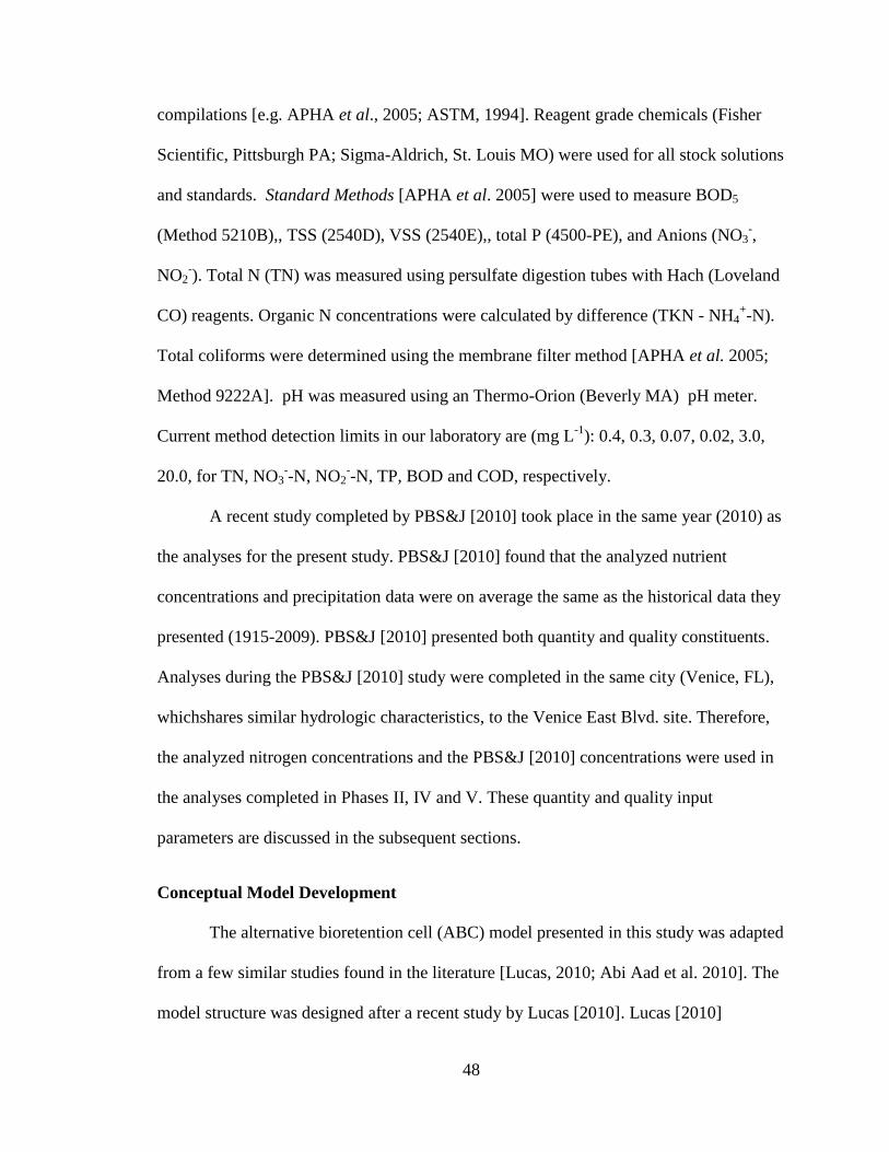
48
compilations [e.g. APHA et al., 2005; ASTM, 1994]. Reagent grade chemicals (Fisher
Scientific, Pittsburgh PA; Sigma-Aldrich, St. Louis MO) were used for all stock solutions
and standards. Standard Methods [APHA et al. 2005] were used to measure BOD5
(Method 5210B),, TSS (2540D), VSS (2540E),, total P (4500-PE), and Anions (NO3-,
NO2-). Total N (TN) was measured using persulfate digestion tubes with Hach (Loveland
CO) reagents. Organic N concentrations were calculated by difference (TKN - NH4+-N).
Total coliforms were determined using the membrane filter method [APHA et al. 2005;
Method 9222A]. pH was measured using an Thermo-Orion (Beverly MA) pH meter.
Current method detection limits in our laboratory are (mg L-1
): 0.4, 0.3, 0.07, 0.02, 3.0,
20.0, for TN, NO3--N, NO2
--N, TP, BOD and COD, respectively.
A recent study completed by PBS&J [2010] took place in the same year (2010) as
the analyses for the present study. PBS&J [2010] found that the analyzed nutrient
concentrations and precipitation data were on average the same as the historical data they
presented (1915-2009). PBS&J [2010] presented both quantity and quality constituents.
Analyses during the PBS&J [2010] study were completed in the same city (Venice, FL),
whichshares similar hydrologic characteristics, to the Venice East Blvd. site. Therefore,
the analyzed nitrogen concentrations and the PBS&J [2010] concentrations were used in
the analyses completed in Phases II, IV and V. These quantity and quality input
parameters are discussed in the subsequent sections.
Conceptual Model Development
The alternative bioretention cell (ABC) model presented in this study was adapted
from a few similar studies found in the literature [Lucas, 2010; Abi Aad et al. 2010]. The
model structure was designed after a recent study by Lucas [2010]. Lucas [2010]
49
thoroughly addresses the conceptual flow of water routing through a layered bioretention
cell. However, Lucas [2010] only analyzed the hydrologic components of a bioretention
cell and did not analyze nutrient transformations. Therefore, the ABC model structure
was adapted for this case study to estimate nitrogen reductions from a system of thirteen
alternative bioretention cells, along Venice East Blvd. in Venice, Florida.
Ammonification was assumed to occur rapidly and completely, so NH4+-N and
Org N are assumed to be a single variable, TKNi. Conversion of both ammonium to
nitrite and nitrite to nitrate was assumed to occur in the aerobic nitrifying (sand) layer.
Conversion of nitrate to nitrogen gas was assumed to occur in the submerged anaerobic
(mulch) layer. Other mechanisms for nitrogen removal, such as adsorption, plant uptake
and volatilization were not considered in this model. However, different nitrogen removal
mechanisms, as well as different types of nutrients and contaminants, can be incorporated
into future updates of this model. A conceptual diagram of the mechanisms for nitrogen
transformation within a bioretention cell is shown in Figure 5.1.

50
Figure 5.1. Conceptual model framework. Depiction shows the flow of stormwater runoff
through a bioretention cell, including the sections where the transformations of each
nitrogen constituent (addressed in this study) were assumed to occur. The symbols are
defined in the subsequent section.
Pond Layer:
Runoff Buildup/ Soil Surface
[Ammonification: OrgN NH4+]
Media Layer- Nitrification: K1, HRT1
[(1) NH4+ + O2 NO2
-; (2) NO2
- + O2 NO3
-
Media Layer- Denitrification: K2, HRT2
NO3-NO2
-NON2ON2
Trench:
Effluent
TKNi, NO3i
Inlet:
Curb Cut
RG1:
Rain
Runoff
Street:
Contributing
Area
TKNi, NO3i
TKNeff, NO3i
NO3-
TKNeff, NO3,eff
Inlet Down:
Surface flow
(Excess Runoff
or Overflow)
Surface

51
The model representing the alternative bioretention cells can be conceptually
“disaggregated” into various components [Lucas, 2010], in order to more accurately
represent the mechanisms for nitrogen removal in each region. SWMM-5 allows for
nutrient inputs into one component to be dependent on the output of the previous
component [Huber and Dickinson, 1988]. Therefore, the nitrification media layer and the
denitrification media layer are linked by nutrient and water flow within the model. This
means that the efficiency of total nitrogen removal within the cell will be dependent on
the efficiency of nitrification and denitrification in the respective media layers. The mass
balances were maintained for both the nitrification and denitrification zone.
Phase II: Analytical Bioretention System Model
First order decay coefficients (k1 and k2) were needed to develop treatment
expressions for the nitrification and denitrification processes occurring in the respective
layers of the alternative bioretention cell (ABC) model. The rate coefficients were
estimated based on the results from a previous study by Ryan Siegel at the University of
Massachusetts, Amherst. Siegel [2009] analyzed a pilot-scale bioretention system (using
wood chips in the denitrification layer), run under laboratory conditions. Siegel [2009]
analyzed synthetic stormwater using nitrogen feed concentrations based on literature
values for urban runoff [Davis et al., 2001; Hsieh and Davis, 2005]. The average influent
feed composition consisted of 1.5 mg/L of NO3--N, 2.1 mg/L of NH4
+-N and 4 mg/L of
Org N. Siegel‟s [2009] laboratory results showed average effluent concentrations for
NO3--N, NH4
+-N and Org N to be < MDL (0.005 mg/L), 0.3 mg/L and 0.6 mg/L,
respectively. The flow rate and duration at which the synthetic stormwater was applied to
the bioretention unit was 240 ml/min and six hours, respectively. The bioretention area
52
was set at 5% of the drainage area being treated, with a runoff coefficient of 0.15 [Siegel,
2009]. The overall mean HRT was estimated at 4.3 hours [Siegel, 2009].
The HRT1 and HRT2 for the nitrification and denitrification layer were estimated
using the known volume and flow values presented by Siegel [2009], using the following
equation:
HRT1 = V1 / Q1*n, for the nitrification layer (5.1)
HRT2 = V2/ Q2*n, for the denitrification layer (5.2)
where, V1 is the volume of nitrification layer, and V2 is the volume of the denitrification
layer in the bioreactor (values obtained from Siegel [2009]).), Q1 and Q2 (Q1 = Q2) are
the flow rate values (obtained from Siegel [2009]), and n is the porosity. Porosity values
for the wood chip and sand media were derived from the literature, as discussed in the
Chapter 6. These porosity values were used with Siegel‟s [2009] data to solve for HRT1
and HRT2 (where HRT1 + HRT2 = 4.3 hours, from Siegel [2009]).
An assumption was made that the nitrification and denitrification layers of
Siegel's system could both be modeled as plug-flow reactors, and that nitrification and
denitrification can both be modeled using first-order reaction kinetics. Therefore, the
nitrification and denitrification layers were modeled as ideal plug flow reactors with first
order reaction kinetics. Based on these assumptions the following equations were used to
solve for k1 and k2.
, for the nitrification layer (5.3)
, for the denitrification layer (5.4)

53
where, and are the rate coefficient values (and are unknown) for nitrification and
denitrification, respectively (1/Time).
Phase III: Hydrologic ABC Model
SWMM-5 simulates the hydrologic and water quality simultaneously; however,
these two models are discussed separately in this study in order to better clarify the
different types of input parameters and their results. In order to develop the ABC model,
the hydrologic data needed to be gathered. The data needed for this phase of the project
was found in the literature, as discussed. The hydrologic model incorporates site-specific
input parameters, as well as hydrologic parameters obtained from the literature. The
hydrologic ABC model assumes:
100% of the impervious flows will be routed to the system
Infiltration rate is set at the SWMM-5 default rate
Fines from the runoff will not clog the system (i.e., adequate maintenance of the
system is assumed)
Hydrologic flows entering the bioretention system will flow through the different
layers of media (until the media is saturated)
The carbon source (wood chips) is assumed to be present in the denitrification
layer during each simulation
Temperature is considered constant at 35° C
Once the ponding elevation of the system has been exceeded (>30.5 cm), the
system will overflow, and excess flows will be sent back into the street, where no
further treatment will occur [Lucas, 2010]

54
The site specific soil infiltration rate parameters were based on soil data found on
the Websoil Survey website [USDA, 2010]. The SWMM-5 model representing an
alternative bioretention cell system (Figure 5.2) is presented to facilitate the comparison
to the conceptual framework (Figure 5.1). Based on the site development plans provided
by Sarasota County, the area of each cell will vary only slightly. The provided plans do
not define the exact area of each cell, therefore making it impossible to calculate the total
area of all the bioretention cells. The plans show each cell individually, and the area of
each cell varies only slightly. Therefore, the model was designed based on the
approximate area of the thirteen cells; by multiplying the approximate area of one cell by
thirteen, to get the total area of the system. Future calibrations could be made to address
the exact area of each cell, if the as-built survey data is provided.
The model was designed so that runoff from the street will flow into the cell
through a cut in the curb. The curb cut is placed approximately 5 cm (0.16 ft) above the
top of the media, to prevent backwash of mulch from the cell [Lucas, 2010]. Runoff that
accumulates in the denitrification (mulch) media layer will collect in the underdrain
which will then discharge into a 61 cm (24 in.) wide overflow compound v-notch weir
116.8 cm (46 in.) higher. The height of the weir was calculated by adding the depth of the
cell (34 in.) to the depth of the ponding layer (12 in.) [Lucas, 2010].

55
Figure 5.2. SWMM 5.0.22 Model of alternative bioretention cell (ABC)

56
Site-specific bioretention cell sizing parameters (e.g. height, width, invert
elevation, etc.) for the ABC model were derived from Sarasota County‟s designs. The
subcatchment, or contributing area, was quantified by finding the total contributing area,
as well as the area of the pervious and impervious potions within the subcatchment. The
input parameters for the area of the subcatchment, in this SWMM-5 model, are based on
the total area and the percent of the area that is impervious. Table 5.2 shows the physical
characteristics for the subcatchment (i.e., the Venice East Blvd. retrofit site).
In the ABC model, each media layer is represented as a storage unit node.
Connecting each storage unit node is an orifice object (i.e., the orifice routes flows into
and out of each storage unit). The orifice object was used by Lucas [2010] to route flows
into the media; this is incorporated in the ABC model to better represent the complexity
of unsaturated flow dynamics into and through a layered bioretention system [Lucas,
2010]. By using a quantity of zero for the width of each orifice, the hydrologic flow
through the bioretention system is modeled so that the orifice does not increase the time it
takes for the runoff to exit the system (the hydraulic residence time, HRT). Table 5.3
defines the storage unit and orifice input parameters needed to calibrate the ABC model.
The outflow (flow leaving the bioretention system) is modeled to exit the system
through a weir (titled the Outflow Weir in this model). The height of the weir is set
higher than the TrenchLayer storage unit, to prevent flows from the street from reentering
the system. According to Lucas [2010], the trench is likely to encounter some infiltration.
Lucas [2010] chose a nominal infiltration rate of 2.54 mm/h (0.10 in/hr); however, this
model ignores the nominal infiltration rate, and assumes no infiltration will occur in the
trench layer. Future calibrations could adjust the infiltration rate in the trench layer.

57
Table 5.2. Physical characteristics of the subcatchment [calculations are based on Doyle
and Miller, 1980; Tsihrintzis and Hamid, 1998].
Characteristic Site: Venice East Blvd.
Low Density Residential
Source for Information
Site Location Venice, Sarasota County,
FL
Case Study
Total Drainage Area
(Subcatchment)
58.39 ac (2,543,289 ft2) USGS [2010]
Width (Subcatchment) 163 ft USGS [2010]
Impervious Area
(Street)
24.62 ac (1,063,094 f2) USGS [2010]
Pervious Area 33.98 ac (1,477,650 f2) Calculated from USGS data
Percent Pervious Area 58.2 % Calculated from USGS data
Percent Impervious
Area
41.8 % Calculated from USGS data
Overland Flow Slope 2.7 % Doyle and Miller [1980];
Tsihrintzis and Hamid
[1998]
Land Use Low Density Residential USGS [2010]
Avg. Lot Size 24 x 30 Doyle and Miller [1980];
Tsihrintzis and Hamid
[1998]
Mean Annual Rainfall
(1915-2010)
98.12 cm/yr PBS&J [2010]
Soil Cover Lawn & Shrubbery Doyle and Miller [1980];
Tsihrintzis and Hamid
[1998]
Soil Description Myakka Fine Sand USGS [2010]
Soil Group (SCS) Fine Sand, poorly drained USGS [2010]
Soil Capacity Approximately 18.03 cm
(0.59 ft)
USGS [2010]
Vegetation Lawn sod w/ garden
shrubbery and trees
Site Evaluation
Street/ Gutter
Description
Curb and gutter Site Evaluation
Current Pervious Area Depressed/ grass swale with
overflow draining to street
Site Evaluation
Proposed Pervious Area Depressed area- drainage
into bioretention cell, and
overflow draining to street
Site Evaluation
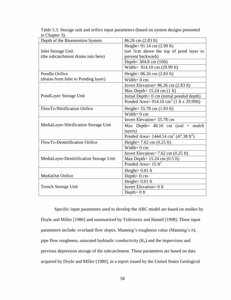
58
Table 5.3. Storage unit and orifice input parameters (based on system designs presented
in Chapter 3).
Depth of the Bioretention System 86.26 cm (2.83 ft)
Inlet Storage Unit
(the subcatchment drains into here)
Height= 91.14 cm (2.99 ft)
(set 5cm above the top of pond layer to
prevent backwash)
Depth= 304.8 cm (10ft)
Width= 914.10 cm (29.99 ft)
PondIn Orifice
(drains from Inlet to Ponding layer)
Height= 86.26 cm (2.83 ft)
Width= 0 cm
PondLayer Storage Unit
Invert Elevation= 86.26 cm (2.83 ft)
Max Depth= 15.24 cm (1 ft)
Initial Depth= 0 cm (initial ponded depth)
Ponded Area= 914.10 cm2 (1 ft x 29.99ft)
FlowTo-Nitrification Orifice Height= 55.78 cm (1.83 ft)
Width= 0 cm
MediaLayer-Nitrification Storage Unit
Invert Elevation= 55.78 cm
Max Depth= 48.16 cm (soil + mulch
layers)
Ponded Area= 1444.14 cm2 (47.38 ft
2)
FlowTo-Denitrification Orifice Height= 7.62 cm (0.25 ft)
Width= 0 cm
MediaLayer-Denitrification Storage Unit
Invert Elevation= 7.62 cm (0.25 ft)
Max Depth= 15.24 cm (0.5 ft)
Ponded Area= 15 ft2
MediaOut Orifice
Height= 0.01 ft
Depth= 0 cm
Trench Storage Unit
Height= 0.01 ft
Invert Elevation= 0 ft
Depth= 0 ft
Specific input parameters used to develop the ABC model are based on studies by
Doyle and Miller [1980] and summarized by Tsihrintzis and Hamid [1998]. These input
parameters include: overland flow slopes, Manning‟s roughness value (Manning‟s n),
pipe flow roughness, saturated hydraulic conductivity (Ks) and the impervious and
pervious depression storage of the subcatchment. These parameters are based on data
acquired by Doyle and Miller [1980], in a report issued by the United States Geological

59
Survey (USGS), for an evaluation of 231 storm events in Southwest Florida. Tsihrintzis
and Hamid [1998] used the data from the USGS report to calibrate a SWMM model for
small urban catchments in Southwest Florida. Doyle and Miller [1980] present all
information relevant to the calibration of the model developed by Tsihrintzis and Hamid
[1998]. These input parameters are shown in Table 5.4. Specific calibration and
verification details are reported in the previous studies by Doyle and Miller [1980] and
Tsihrintzis and Hamid [1998]. The average capillary suction head, initial moisture deficit
and saturated hydraulic conductivity are not applicable at the wetting front in the ABC
model, as flows route to the subsequent storage unit (i.e., flow does not infiltrate into the
underlying soil).
The ABC model presented in this study, to predict post-development nitrogen
concentrations for the Venice East Blvd. bioretention cell retrofit site, is based in part on
the SWMM calibration data presented by Tsihrintzis and Hamid [1998]. This is because
the SWMM model presented by Tsihrintzis and Hamid [1998] was designed after a site in
SW Florida, only a few hours away from the Venice, FL study site. Therefore, it is
assumed that these sites will share identical hydrological and physical characteristics.
Detailed descriptions of the SWMM calibration process and precipitation data (including
single-event rainfall data) are discussed in detail by Tsihrintzis and Hamid [1998].
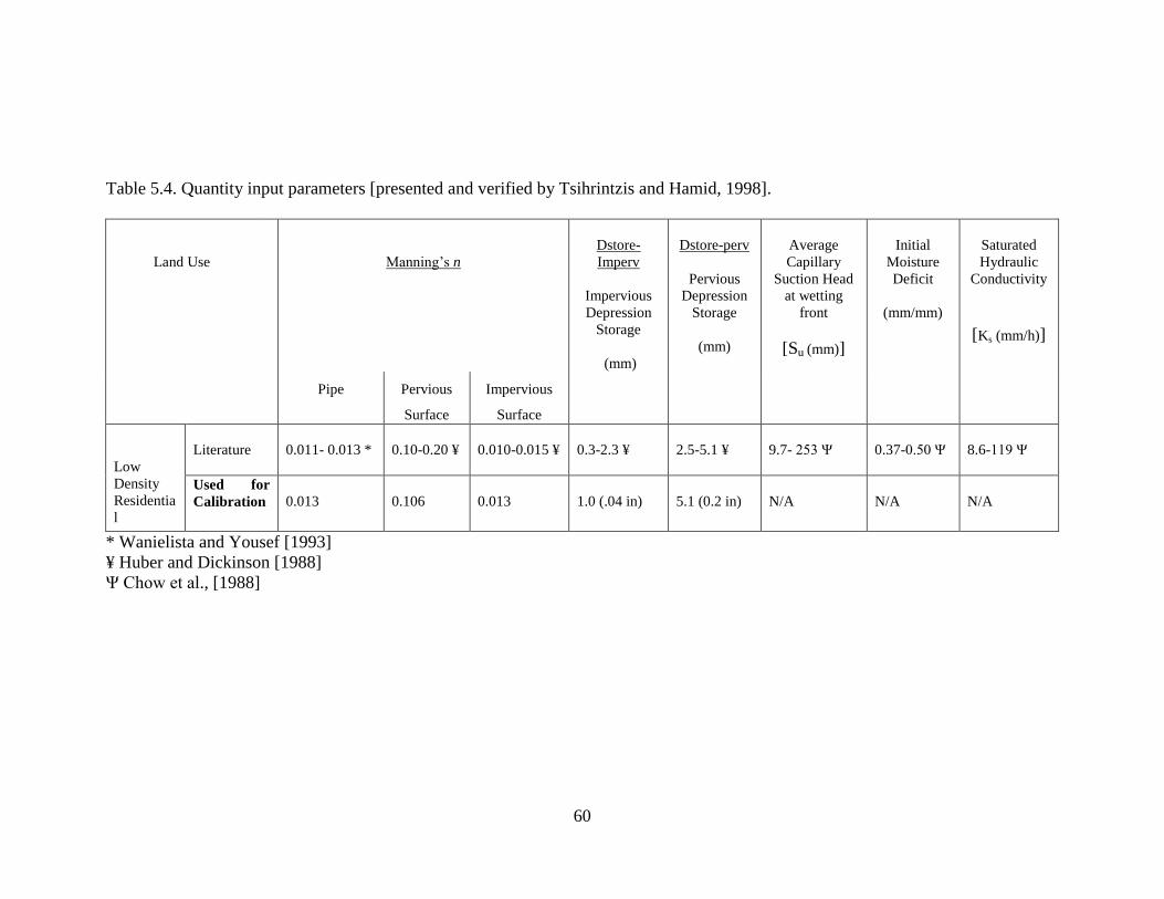
60
Table 5.4. Quantity input parameters [presented and verified by Tsihrintzis and Hamid, 1998].
Land Use
Manning‟s n
Dstore-
Imperv
Impervious
Depression
Storage
(mm)
Dstore-perv
Pervious
Depression
Storage
(mm)
Average
Capillary
Suction Head
at wetting
front
[Su (mm)]
Initial
Moisture
Deficit
(mm/mm)
Saturated
Hydraulic
Conductivity
[Ks (mm/h)]
Pipe Pervious
Surface
Impervious
Surface
Low
Density
Residentia
l
Literature
0.011- 0.013 *
0.10-0.20 ¥
0.010-0.015 ¥
0.3-2.3 ¥
2.5-5.1 ¥
9.7- 253 Ψ
0.37-0.50 Ψ
8.6-119 Ψ
Used for
Calibration
0.013
0.106
0.013
1.0 (.04 in)
5.1 (0.2 in)
N/A
N/A
N/A
* Wanielista and Yousef [1993]
¥ Huber and Dickinson [1988]
Ψ Chow et al., [1988]
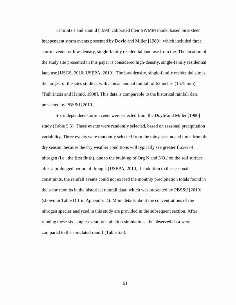
61
Tsihrintzis and Hamid [1998] calibrated their SWMM model based on sixteen
independent storm events presented by Doyle and Miller [1980]; which included three
storm events for low-density, single-family residential land use from the. The location of
the study site presented in this paper is considered high-density, single-family residential
land use [USGS, 2010; USEPA, 2010]. The low-density, single-family residential site is
the largest of the sites studied, with a mean annual rainfall of 63 inches (1575 mm)
[Tsihrintzis and Hamid, 1998]. This data is comparable to the historical rainfall data
presented by PBS&J [2010].
Six independent storm events were selected from the Doyle and Miller [1980]
study (Table 5.5). These events were randomly selected, based on seasonal precipitation
variability. Three events were randomly selected from the rainy season and three from the
dry season, because the dry weather conditions will typically see greater fluxes of
nitrogen (i.e., the first flush), due to the build-up of Org N and NO3- on the soil surface
after a prolonged period of drought [USEPA, 2010]. In addition to the seasonal
constraints, the rainfall events could not exceed the monthly precipitation totals found in
the same months in the historical rainfall data; which was presented by PBS&J [2010]
(shown in Table D.1 in Appendix D). More details about the concentrations of the
nitrogen species analyzed in this study are provided in the subsequent section. After
running these six, single-event precipitation simulations, the observed data were
compared to the simulated runoff (Table 5.6).

62
Table 5.5. Model quantity calibration data: single-family residential site [based on
findings presented by Doyle and Miller, 1980].
Storm #
Storm Date Time Interval Rainfall
(in)
Observed
Runoff (in.)
Observed Peak
Q (ft3/sec)
1 01-13-74 0720-0990 0.810 0.0980 2.82
3 04-15-74 0364-0480 0.600 0.0590 3.79
45 12-26-74 1271-1380 0.140 0.0100 0.570
57 06-17-74 0667-0840 1.25 0.0840 32.8
73 07-19-74 0305-0630 1.92 0.400 22.1
84 09-18-74 0860-1440 4.37 0.800 27.1
Phase IV: Water Quality ABC Model
The design of the water quality ABC model was developed using the following
assumptions:
100% Conversion of OrgN NH4+ occurs in the Ponding Layer
All nitrification occurs in the nitrification layer, all denitrification in the
denitrification layer.
Nitrite was considered an intermediary species; therefore, all nitrite/nitrate in the
system was available for decomposition.
Denitrification will occur at micro-sites within the anoxic bioflim layer associated
with the denitrification media; therefore, the dissolved oxygen concentration in
the bulk liquid is ignored (i.e., denitrification will occur)
Plant uptake, volatilization and adsorption are not considered in this model (i.e.,
only nitrification and denitrification are considered)

63
In N removing bioretention cells, total N removal can occur in the following
steps: adsorption and filtration of Org N and adsorption of NH4+ during the wetting
period, ammonification of retained Org N and nitrification of NH4+ as oxygen reenters
the pores during the drying period, and denitrification in the submerged zone during
subsequent wetting periods utilizing the solid substrate wood (e.g. mulch) as the electron
donor [Ergas et al., 2010]. In the ABC model, only nitrification and denitrification are
considered. Based on the literature, for low-density residential neighborhoods, the most
relevant sources of nitrogen for this project will be Org N, NH4+-N, and NO3
--N
[USEPA, 2010], NO2- concentrations were assumed negligible. Considering TKN is the
sum of Org N and NH4+-N, TKN was tracked in SWMM-5 as well as NO3
--N.
The following treatment expressions were used to evaluate the mass (lbs/event) of
TKN and NO3--N in the effluent.
, for the nitrification layer (5.5)
, for the denitrification layer (5.6)
where, . is the mass of the reacted, found in equation 5.5 (i.e., the
), k1 and k2 are the rate loss coefficient values estimated in
Phase II. Equation 5.5 was used in the treatment expression dialog box in SWMM-5, in
the nitrification layer of the ABC model. Using a defined TKNi concentration (mg/L),
with the treatment expression (equation 5.5) input into the nitrification layer, SWMM-5
quantified the reacted TKN (lbs/event). The method for estimating NO3- removal using
the ABC model is described below.

64
SWMM-5 was able to solve for the removal of TKNi (R_TKNi) during simulation
runs. However, it could not directly solve for the removal of NO3-. In order to solve
equation 5.6, the volume and flow were divided at each time step (30 minute interval) to
find the HRT in the denitrification layer at each time step. The HRT at each time step was
then used to solve equation 5.6 (at each time step). SWMM-5 gives TKNi, R_TKNi, and
NO3- in lbs/event. This number represents flow multiplied by the concentration. The
TKNi and NO3- loads (lbs/event) were then found for each concentration shown in Table
5.6. Solving equation 5.6, the results were used to find the average pollutant removal
efficiency for the EPA Sarasota sized ABC systems for each event, for the four
concentrations shown in Table 5.6. Once the average pollutant removal efficiencies were
found, the TN load reduction was derived, including the TN removal rates for both the
EPA and Sarasota sized ABC systems.
The precipitation data presented in the previous section were analyzed at a
different site (in SWFL) from where the site-specific nitrogen concentrations were
analyzed in Phase I; therefore, it was necessary to simulate each nitrogen concentration as
a sampling distribution. The uncertainty for each parameter is specified by using a
minimum, median, maximum and observed value. The benefit of using a range of
nitrogen concentrations is that, it allows for a less site-specific model (i.e., the results can
be used to estimate loading rates at various sites across SWFL, assuming the sites share
similar physical characteristics). The range of nitrogen concentrations used for simulating
loading from the stormwater runoff are presented in Table 5.6. The concentrations used
are based on the concentrations seen in both the PBS&J [2010] study and the field
sampling done during this study.

65
Table 5.6. Nitrogen species in runoff; used to calibrate the SWMM-5 model [adapted
from PBS&J, 2010 and field sampling data].
Constituent
Minimum
Concentration
(mg/L)
Median
Concentration
(mg/L)
Maximum
Concentration
(mg/L)
Analyzed
Concentration
(mg/L)
NO2-/NO3
-
0.000
0.420
1.80
1.48
NH4+-N
0.010
0.310
1.22
1.55
Org N
0.350
5.28
15.9
1.38

66
Chapter Six:
Results and Discussion
Phase I: Site-Specific Nutrient Characterization Results
For two separate storm events I analyzed the analytes shown in Table 6.1 at the
Venice East Blvd. bioretention retrofit site, in order to quantify the pre-developed
nutrient characteristics. Both storm events occur in the dry season; November 14th
and
December 11th
. The average concentrations for the various parameters measured are
shown in Table 6.1. The standard deviations from the average values are shown in
parentheses.
Table 6.1 Results of November 4th
and December 11th
, 2010 stormwater runoff samples.
Analyte November 4th
Concentration
December 11th
Concentration
Units
TN 1.70 (0.170) 1.30 (0.660) mg/L
TP 0.11 (0.020) 0.170 (0.010) mg/L
NO2-/NO3
- 0.570 (0.450) 0.430 (0.190) mg/L
Total Coliforms 27.0 (4.71) 24.0 (3.17) CFU/100 mL
pH 7.89 (0.190) 7.53 (0.510) 0-14 pH units
DO 6.55 (0.290) 7.21 (4.42) mg/L
BOD5 4.70 (1.29) 3.87 (0.340) mg/L
TSS 22.2 (3.15) 28.7 (0.490) mg/L
VSS 11.2 (2.41) 16.3 (0.140) mg/L
*Standard deviations given in (). Triplicates samples were used during analyses to
determine the standard deviations.

67
The results from the laboratory analyses indicate that there was a greater
concentration of TN seen in the November 4th
analysis, compared to the December 11th
analysis. Although hydrologic data were not quantified during these two events, it was
noted that the November 4th
event was much more intense and last approximately 6
hours. In comparison, the December 11th
event was a very mild storm event, with rainfall
only lasting approximately 2 hours. The results from this Phase compared well with the
typical concentrations found in the literature (Table 4.1).
Phase II: Analytical Bioretention System Model Results
Results from a pilot-scale bioretention system, run under laboratory controlled
conditions, were used to estimate the mean HRT1 (for nitrification) and the mean HRT2
(for denitrification), as discussed in Chapter 5. The porosity of sand and wood chip was
assumed to be 0.25 and 0.25, respectively [Robertson, 2010; Ima and Mann, 2007].
Although the literature defined the porosity of wood chips to be between 0.45 and 0.63
[Ima and Mann, 2007], the 0.25 porosity value was chosen so that the HRT of the system
would be equal to the 4.3 hours found by Siegel [2009]. The literature notes that wood
chip porosity varies greatly depending on the type of wood, the size of the chips and
whether the wood was moist prior to the pulse tracer study [Ima and Mann, 2007]. Using
these porosity values and the volume and flow presented by Siegel [2009], the estimated
mean HRT1 value for the nitrification layer was 2.87 hours, and the estimated mean
HRT2 value for the denitrification layer was 1.43 hours.
Using these HRT values to solve equations 5.3 and 5.4, the reaction rate
coefficients for nitrification and denitrification were found to be 0.70/hour and 5.2/hour,
respectively. A recent study found similar k-values for the rate of denitrification,

68
0.19/min [Warneke et al., 2011]. As the reaction rate of denitrification is dependent on
other variables besides the HRT (e.g. temperature, dissolved oxygen concentration,
surface areas, moisture content, electron donor availability, etc.), the k-values estimated
during Phase II of this study seem to compare well to the literature [Warneke et al., 2011;
Greenan et al., 2006, 2009; Groffman et al., 2006].
Phase III: Hydrologic ABC Model Results
Lucas [2010] discusses that designing the model with this disaggregated routing
leads to “unexpected behavior” during simulation events, as the “various compartments
fill and empty at different rates”. Results from the simulations for the six separate storm
events modeled for this study also showed this same unexpected behavior; however, the
hydrologic behavior seemed a bit extreme when comparing results with Lucas [2010],
due to the sharp flow peaks seen in the various compartments of the system (Figure 6.1).
These peaks result from the continuous filling and draining of the inadequately sized
pond layer. The September 18th
, storm event was 4.37 inches (the largest storm event
simulated) over nine and a half hours. Most of the flow during this event was routed to
the curb lower orifice, and did not enter the system. After careful deliberation, it was
discovered that the Sarasota bioretention system design area was sized at only 1% of the
total drainage area. The system being sized this small was affecting the hydrologic
performance of the model.
To confirm the validity of these results, a new ABC model was designed based on
the bioretention cell sizing specifications defined by the EPA (bioretention system area
should be approximately 5-7% of the drainage basin area) [USEPA, 2000]. The resized
ABC model was designed with a larger area, which was designed at approximately 6% of

69
the subcatchment area. The hydrologic results and nutrient transformations in the ABC
model based on EPA sizing guidelines showed much better results for storm events
exceeding 1 inch. Hydrologic performance of the ABC model designed based on the
sizing specifications defined by the USEPA are presented in Figure 6.2 to facilitate
comparison to the ABC model design based on Sarasota County‟s plans; the results in
Figure 6.2 also compare nicely with the results presented by Lucas [2010].
Figure 6.1. Flow through the orifice controlled system for a 4.37-in. simulated storm
event for system sized according to Sarasota‟s plans.
0
0.2
0.4
0.6
0.8
1
1.2
0 8 16 24 32
Flo
w (
L/se
c)
Time (hr.)
Flow to Pond Layer
9/18/1974
0
0.5
1
0 8 16 24 32
Flo
w (
L/se
c)
Time (hr.)
Nitrification Layer Inflow
9/18/1974
0 0.5
1 1.5
2 2.5
0 8 16 24 32
De
pth
(ft
.)
Time (hr.)
Nitrification Layer Depth
9/18/1974
0 0.05
0.1 0.15
0.2 0.25
0.3 0.35
0 8 16 24 32
Flo
w (
L/se
c)
Time (hr.)
Denitrification Inflow
9/18/1974
0
1
2
3
4
0 8 16 24 32
De
pth
(ft
.)
Time (hours)
Denitrification Layer Depth
9/18/1974
0
0.05
0.1
0.15
0.2
0 8 16 24 32
Flo
w (
L/se
c)
Time (hr.)
Trench Inflow
9/18/1974

70
Figure 6.2. Flow through the orifice controlled system for a 4.37-inch simulated storm
event in system sized according to USEPA guidelines.
Simulations were run to compare effluent quantity using infiltration rates defined
by Lucas [2010] in each of the storage unit/layers. Results from these simulations showed
that no substantial difference in hydraulic performance. Site-specific infiltration rates
were not defined in this study. Considering results were relatively identical with or
without infiltration rates being defined in the storage units, infiltration rates into the
surrounding soils of each storage unit layer were ignored in both of the final ABC models
(the Sarasota sized system and the redesigned, larger system). In the future, assuming
infiltration rates are available, it may be useful to define infiltration rates for each storage
unit/layer.
The results show that more runoff routed through the larger system than the
smaller system, and the overall maximum HRT of the larger system was substantially
greater (by almost 2 days), then the overall maximum HRT in the smaller system. Based
0
1
2
3
4
5
0 2 4 6 8 10
Flo
w (
L/se
c)
Time (hr.)
Flow to Pond Layer
9/18/1974
0 1 2 3 4 5
0 2 4 6 8 10
Flo
w (
L/se
c)
Time (hr.)
Nitrification Layer Inflow
9/18/1974
0
0.5
1
1.5
2
0 8 16 24
De
pth
(ft
)
Time (hr.)
Nitrification Layer Depth
9/18/1974
0
0.1
0.2
0.3
0.4
0 10 20 30 40
Flo
w (
L/se
c)
Time (hr.)
Denitrification Inflow
9/18/1974
0
1
2
3
0 20 40
De
pth
(ft
.)
time (hours)
Denititrification Layer Depth
9/18/1974
0
0.02
0.04
0.06
0.08
0 40 80
Flo
w (
L/se
c)
Time (hr.)
Trench Inflow
9/18/1974

71
on these simulated HRT values, it was no surprise that the efficiency to achieve
nitrification and denitrification was much better in the larger system, than in the smaller.
Phase IV: Water Quality ABC Model Results
Six simulations were run in SWMM-5 for the six separate storm events using a
range of concentrations (Table 5.6). The minimum TKNeff and NO3-eff concentrations
(mg/L) vs. time (hours) from the nitrification layer are shown in the Figures below for the
Sarasota sized ABC model (Figure 6.3) and the EPA sized ABC model (Figure 6.4), for
the 4.37-inch simulated storm event. These graphs show a peak of TKNeff (less than 0.36
mg/L) as the flow enters the denitrification layer (when the HRT is too short and does not
allow for efficient nitrification transformations). Due to the smaller size of the ponding
layer in the Sarasota sized ABC model, the TKNeff has completely passed through the
denitrification layer much more rapidly than it has in the EPA sized ABC model. In
addition, the increased time interval in the EPA sized ABC model is due to the fact that
more stormwater runoff has infiltrated into the EPA sized ABC model, because of its
larger size. Therefore, these flows take longer to drain out of the system completely.
Figure 6.3. TKNeff and NO3-eff concentrations vs. time in Sarasota sized model.
0
0.2
0.4
0 5 10
Co
nce
ntr
atio
n …
Time (hours)
TKNeff (mg/L) from Nitrification Layer
9/18/1974
0
0.1
0 5 10
Co
nce
ntr
atio
n …
Time (hours)
NO3 (mg/L) in Nitrification Layer
9/18/1974
0
5
10
15
0.0 5.0 10.0
Co
nce
ntr
atio
n …
Time (hours)
NO3eff (mg/L) in Denitrification Layer
9/18/1974

72
Figure 6.4. TKNeff and NO3-eff concentrations vs. time in EPA sized model.
The pre-development event loading rates for the six separate storm events were
simulated in SWMM-5. The results from these six separate event simulations are shown
for the TKN loading rates (Table 6.2), and for the event NO3- loading rates (Table 6.3).
During the dry season, it is probably unrealistic to assume that you would see minimum
concentrations of nitrogen in stormwater runoff. Generally, after long dry periods,
nutrients build up on the ground surface; therefore, it is likely that nitrogen loading rates
would be closer to the median event loading rate. In comparison, it is probably unrealistic
to assume that during the rainy season you would see the maximum nitrogen loading
rates. Typically, wet weather flushes the nutrients off the soil surface; therefore, during
wet years, you would likely see concentrations closer to the minimum event loading
rates. If the results were shown as annual N loading rates, using a range of concentrations
would result in unrealistic outcomes. Therefore, the annual N loads were not calculated in
this study.
0
0.2
0.4
0 10 20 30 40
Co
nce
ntr
atio
n …
Time (hours)
TKNeff (mg/L) from Nitrification Layer
9/18/1974
0
0.1
0 5 10
Co
nce
ntr
atio
n …
Time (hours)
NO3 (mg/L) in Nitrification Layer
9/18/1974
0
5
10
15
0.0 5.0 10.0
Co
nce
ntr
atio
n …
Time (hours)
NO3eff (mg/L) in Denitrification Layer
9/18/1974

73
Table 6.2. SWMM-5 simulated pre-development TKN loading rates for six separate
storm events.
Event Rainfall
(in)
Event
loading rate
(lbs)
assuming
minimum
TKN conc.
Event
loading rate
(lbs)
assuming
median
TKN conc.
Event
loading rate
(lbs)
assuming
maximum
TKN conc.
Event
loading rate
(lbs)
assuming
analyzed
TKN conc.
1/13/1974 0.810 1.93 29.3 91.8 15.7
4/15/1974 0.600 1.43 22.2 68.0 11.6
6/17/1974 0.140 0.330 5.17 15.9 2.71
7/19/1974 1.25 2.98 46.2 132 24.2
79/18/1974 1.92 4.95 71.0 218 37.2
12/26/1974 4.37 10.4 161 495 84.6
Table 6.3. SWMM-5 simulated pre-development NO3- loading rates for six separate
storm events
Event Rainfall
(in)
Event
loading rate
(lbs)
assuming
minimum
NO3- conc.
Event
loading rate
(lbs)
assuming
median
NO3- conc.
Event
loading rate
(lbs)
assuming
maximum
NO3- conc,
Event
loading
rate (lbs)
assuming
analyzed
NO3- conc.
1/13/1974 0.810 0.000 2.25 9.64 7.93
4/15/1974 0.600 0.000 1.67 7.14 5.87
6/17/1974 0.140 0.000 0.39 1.67 1.37
7/19/1974 1.25 0.000 3.47 14.9 12.2
79/18/1974 1.92 0.000 5.33 22.9 18.8
12/26/1974 4.37 0.000 12.12 52.0 47.7
By inputting equation (5.5) into the nitrification layer, SWMM-5 estimated the
efficiency of the system to achieve nitrification (Tables 6.4 through 6.7). SWMM-5
output data from these simulations can be found in Appendix D. The mass TKNi that
reacted is about the same for each simulation. Therefore showing results are consistent
for each simulation. The denitrification results are discussed in detail in the following
paragraphs.

74
Table 6.4. Simulated efficiency of nitrification in ABC models, for the six storm events
analyzed at the minimum nitrogen concentration.
Event System TKNi
(lbs)
Average
Mass
Reacted
(%)
Average
TKN,
effluent
(lbs)
Average TKN
load reduction
(lbs/event)
1/13/1974 Sarasota Sized 0.76 0.34 0.50 0.26
EPA Sized 0.76 1.0 0.00 0.76
4/15/1974 Sarasota Sized 0.55 0.44 0.31 0.24
EPA Sized 0.55 1.0 0.00 0.55
6/17/1974 Sarasota Sized 1.2 0.23 0.93 0.27
EPA Sized 1.2 0.81 0.23 0.97
7/19/1974 Sarasota Sized 1.9 0.17 1.6 0.31
EPA Sized 1.9 0.66 0.63 1.2
9/18/1974 Sarasota Sized 4.3 0.12 3.8 0.50
EPA Sized 4.3 0.54 2.0 2.3
12/26/1974 Sarasota Sized 0.09 1.0 0.00 0.09
EPA Sized 0.09 1.0 0.00 0.09 *Minimum nitrogen concentration: TKNi= 0.36 mg/L, NO3
--N= 0 mg/L
Table 6.5. Simulated efficiency of nitrification in ABC models, for the six storm events
analyzed at the median nitrogen concentration.
Event System TKNi
(lbs)
Average
Mass
Reacted
(%)
Average
TKN,
effluent
(lbs)
Average TKN
load reduction
(lbs/event)
1/13/1974 Sarasota Sized 12 0.34 7.7 4.3
EPA Sized 12 1.0 0.00 12
4/15/1974 Sarasota Sized 9.0 0.45 4.8 4.2
EPA Sized 9.0 1.0 0.00 9.0
6/17/1974 Sarasota Sized 19 0.14 14 5.0
EPA Sized 19 0.81 3.6 15
7/19/1974 Sarasota Sized 30 0.17 24 6.0
EPA Sized 30 0.66 9.8 20
9/18/1974 Sarasota Sized 67 0.12 59 8.0
EPA Sized 67 0.54 31 36
12/26/1974 Sarasota Sized 1.4 1.0 0.00 1.4
EPA Sized 1.4 1.0 0.00 1.4 *Median nitrogen concentration: TKNi= 5.39 mg/L, NO3
--N= 0.42 mg/L
75
Table 6.6. Simulated efficiency of nitrification in ABC models, for the six storm events
analyzed at the maximum nitrogen concentration.
Event System TKNi
(lbs)
Average
Mass
Reacted
(%)
TKN,
effluent
(lbs)
Average TKN
load reduction
(lbs/event)
1/13/1974 Sarasota Sized 36 0.34 24 12
EPA Sized 36 1.0 0.00 36
4/15/1974 Sarasota Sized 26 0.43 15 11
EPA Sized 26 1.0 0.00 26
6/17/1974 Sarasota Sized 57 0.23 44 13
EPA Sized 57 0.81 11 46
7/19/1974 Sarasota Sized 89 0.17 74 15
EPA Sized 89 0.66 30 59
9/18/1974 Sarasota Sized 204 0.12 180 24
EPA Sized 205 0.54 95 110
12/26/1974 Sarasota Sized 4.3 1.0 0.00 4.3
EPA Sized 4.3 1.0 0.00 4.3 *Maximum nitrogen concentration: TKNi= 17.14 mg/L, NO3
--N= 1.8 mg/L
Table 6.7. Simulated efficiency of nitrification in ABC models, for the six storm events
analyzed at the analyzed nitrogen concentration.
Event System TKNi
(lbs)
Average
Mass
Reacted
(%)
TKN,
effluent
(lbs)
Average TKN
load reduction
(lbs/event)
1/13/1974 Sarasota Sized 6.2 0.34 4.1 2.1
EPA Sized 6.2 1.0 0.00 6.2
4/15/1974 Sarasota Sized 4.5 0.44 2.5 2.0
EPA Sized 4.5 1.0 0.00 4.5
6/17/1974 Sarasota Sized 9.7 0.23 7.5 2.2
EPA Sized 9.7 0.81 1.9 7.8
7/19/1974 Sarasota Sized 15 0.17 13 2.0
EPA Sized 15 0.66 5.1 9.9
9/18/1974 Sarasota Sized 35 0.12 31 4.0
EPA Sized 35 0.54 16 19
12/26/1974 Sarasota Sized 0.73 1.0 0.00 0.73
EPA Sized 0.73 1.0 0.00 0.73 *Analyzed nitrogen concentration: TKNi= 2.93 mg/L, NO3
--N= 1.48 mg/L

76
The results presented in Table 6.4-6.7 show that the mean percent of TKN reacted
in the Sarasota sized ABC model was 38%, compared to a mean of 84% in the EPA sized
system. The December 26th
storm event was the lightest rain event of all six storm events;
only 0.14 inches of rain. When comparing the results of the December 26th
simulation,
the output data shows that both the Sarasota and EPA sized ABC models were capable of
achieving 100% conversion of the TKN. However, the results shown that for the other
five rain events the EPA sized ABC model was much more efficient at achieving
nitrification.
The rate of denitrification was not directly solved by the ABC model. The HRT
was estimated based on the SWMM-5 output data, for each storm event (discussed in
Chapter 5). The reacted TKN concentration (R_TKNi) was combined with the NO3i--N
concentration, in order to estimate the concentration of NO3--N coming into the
denitrification layer. Appendix D shows detailed SWMM-5 output data used to solve
equation 5.6. The estimated HRT values for each time step were then used to solve the
first-order denitrification reaction (equation 5.6) and the percent mass that reacted for
each time step. The average percent mass reacted was then used to estimate the average
event load reduction (lbs/event). The results from these calculations are presented in
Tables 6.8-6.11. The results from this Phase of the study indicate that the EPA sized ABC
system would achieve on average the highest rates of nitrification (84%), and saw overall
nitrogen removal rates (lbs/event) by as much as 87% (Tables 6.8-6.11). Although both
systems were capable of achieving the same (on average) denitrification rates (96%), the
EPA sized system reduced a much larger overall mass of total nitrogen (lbs/event) than
the Sarasota sized system.

77
Table 6.8. Simulated efficiency of denitrification in ABC models, for the six storm events
analyzed at the minimum nitrogen concentration.
Event System NO3i
(lbs)
Average
Mass
Reacted
(%)
Average
NO3,
effluent
(lbs)
Average
NO3- load
reduction
(lbs/event)
Average
TN load
remaining
(lbs/event)
1/13/1974 Sarasota Sized 0.26 0.96 0.01 0.25 0.51
EPA Sized 0.76 0.96 0.03 0.73 0.73
4/15/1974 Sarasota Sized 0.24 0.96 0.01 0.23 0.47
EPA Sized 0.55 0.96 0.02 0.53 0.53
6/17/1974 Sarasota Sized 0.27 0.97 0.01 0.26 0.53
EPA Sized 0.97 0.97 0.03 0.94 0.94
7/19/1974 Sarasota Sized 0.31 0.96 0.01 0.30 0.61
EPA Sized 1.2 0.96 0.04 1.2 1.2
9/18/1974 Sarasota Sized 0.50 0.96 0.01 0.48 0.48
EPA Sized 2.3 0.96 0.09 2.2 2.2
12/26/1974 Sarasota Sized 0.09 0.96 0.00 0.09 0.09
EPA Sized 0.09 0.96 0.00 0.09 0.09 *Minimum nitrogen concentration: TKNi= 0.36 mg/L, NO3
--N= 0 mg/L
Table 6.9. Simulated efficiency of denitrification in ABC models, for the six storm events
analyzed at the median nitrogen concentration.
Event System NO3i
(lbs)
Average
Mass
Reacted
(%t)
Average
NO3,
effluent
(lbs)
Average
NO3- load
reduction
(lbs/event)
Average
TN load
remaining
(lbs/event)
1/13/1974 Sarasota Sized 4.9 0.96 0.12 4.7 5.1
EPA Sized 13 0.96 0.50 12 12
4/15/1974 Sarasota Sized 4.4 0.96 0.18 4.2 4.7
EPA Sized 9.2 0.96 0.37 8.8 9.3
6/17/1974 Sarasota Sized 5.6 0.97 0.17 5.4 6.2
EPA Sized 16 0.97 0.48 16 16
7/19/1974 Sarasota Sized 7.0 0.96 0.28 6.7 7.9
EPA Sized 21 0.96 0.84 20 22
9/18/1974 Sarasota Sized 13 0.96 0.53 12 12
EPA Sized 41 0.96 1.64 39 39
12/26/1974 Sarasota Sized 1.5 1.0 0.00 1.5 1.5
EPA Sized 1.5 1.0 0.00 1.5 1.5 *Median nitrogen concentration: TKNi= 5.39 mg/L, NO3
--N= 0.42 mg/L

78
Table 6.10. Simulated efficiency of denitrification in ABC models, for the six storm
events analyzed at the maximum nitrogen concentration.
Event System NO3i
(lbs)
Average
Mass
Reacted
(%)
Average
NO3,
effluent
(lbs)
Average
NO3- load
reduction
(lbs/event)
Average
TN load
remaining
(lbs/event)
1/13/1974 Sarasota Sized 16 0.96 0.64 15 15
EPA Sized 40 0.96 1.6 38 38
4/15/1974 Sarasota Sized 14 0.96 0.56 13 13
EPA Sized 30 0.96 1.2 29 38
6/17/1974 Sarasota Sized 19 0.95 0.95 18 18
EPA Sized 52 0.97 1.6 50 50
7/19/1974 Sarasota Sized 24 0.96 0.96 23 23
EPA Sized 68 0.96 2.7 65 66
9/18/1974 Sarasota Sized 40 0.96 1.6 38 44
EPA Sized 131 0.96 5.2 126 130
12/26/1974 Sarasota Sized 4.7 0.96 0.19 4.5 4.6
EPA Sized 4.7 0.96 0.19 4.5 4.6 *Maximum nitrogen concentration: TKNi= 17.14 mg/L, NO3
--N= 1.8 mg/L
Table 6.11. Simulated efficiency of denitrification in ABC models, for the six storm
events analyzed at the analyzed nitrogen concentration.
Event System NO3i
(lbs)
Average
Mass
Reacted
(%)
Average
NO3,
effluent
(lbs)
Average
NO3- load
reduction
(lbs/event)
Average
TN load
remaining
(lbs/event)
1/13/1974 Sarasota Sized 5.3 0.96 0.21 5.0 5.6
EPA Sized 11 0.96 0. 44 11 11
4/15/1974 Sarasota Sized 4.3 0.96 0.17 4.2 4.4
EPA Sized 9.5 0.96 0.38 9.1 9.7
6/17/1974 Sarasota Sized 7.3 0.97 0.22 7.1 7.4
EPA Sized 13 0.97 0.39 13 14
7/19/1974 Sarasota Sized 10 0.96 0.40 9.6 9.9
EPA Sized 18 0.96 0.72 17 19
9/18/1974 Sarasota Sized 22 0.96 0.88 21 22
EPA Sized 37 0.96 1.5 36 38
12/26/1974 Sarasota Sized 1.1 0.96 0.04 1.1 1.2
EPA Sized 1.1 0.96 0.04 1.1 1.2 *Analyzed nitrogen concentration: TKNi= 2.93 mg/L, NO3
--N= 1.48 mg/L

79
Chapter Seven:
Conclusions
The overall goal of this research project was to estimate nitrogen removal from
stormwater runoff for a proposed alternative bioretention system in Venice, FL. The
development and calibration of the ABC model took place in four separate phases. Phase
I was the quantification of quantity and quality input parameters, which were based on
site-specific analyses and the literature. Phase II used analytical methods to derive the
rate coefficients for nitrification and denitrification. Phase III and IV was running
simulations in SWMM-5 to estimate the quantity and quality of the effluent from the
proposed bioretention system.
Phase II of ABC model development was based on previous research conducted
by Ryan Siegel, at the University of Massachusetts, Amherst in June 2008. The results of
this research were used to determine first order rate coefficients for nitrification and
denitrification. These values were then used in the treatment expressions needed to
calibrate the SWMM-5 model. Based on the hydraulic residence time determined by
Siegel, the nitrification and denitrification first order rate coefficients were determined to
be 0.70/hour and 5.2/hour, respectively.
Upon completion of Phase I and II, the ABC model was developed in SWMM-5,
and used to run quantity and quality simulations for Phases III and IV. The results of
these simulations were used to compare the annual nitrogen loading rates of the post-

80
developed bioretention system site to the pre-developed site. The results from these
simulations showed that the system was experiencing flooding in the various
compartments of the system for simulated rain events that exceeded 1-inch. These results
led to the evaluation of the hydrologic performance of the ABC model (designed after
plans provided by Sarasota County).
A new model was developed to compare the performance with the model
designed after Sarasota County‟s specifications. The new model was designed with a
total area equal to 6% of the subcatchment area. The larger sized (6%) ABC model and
smaller sized (1%) ABC model were then used to simulate the same quantity and quality
results. The results from both the Sarasota sized system and the redesigned system (based
on EPA‟s bioretention sizing guidelines; 5% of the impervious portion of the
subcatchment) were then used to compare to annual loading rates of the post-developed
bioretention site to the pre-developed site. Comparing the simulation results from both
models showed that the larger bioretention system performed better hydraulically than
the smaller system. The results showed that more runoff routed through the larger system
than the smaller one, and the maximum HRT of the larger system was substantially
greater (by almost 2 days), then the maximum HRT in the smaller system. Based on the
simulated HRT values, it was no surprise that the efficiency to achieve nitrification and
denitrification was much better in the larger system, than in the smaller.
Overall, the EPA sized system achieved a nitrification rate of 84%, in comparison
to only a rate 38% in the Sarasota sized system. The results from this study compare well
to similar studies evaluating the performance of bioretention systems (for field-scale
bioretention systems) [Ergas et al., 2010; Davis et al., 2006]. Both systems achieved the
81
same rate of denitrification, 96% on average. However, the EPA sized ABC model
reduced TN by as much as 87%, compared to the Sarasota sized system, which saw TN
reductions of as much as 56%. The results from this research indicate that future design
of these alternative bioretention systems should include careful planning to ensure that
the area of the alternative bioretention system is close to the EPA‟s guidelines; 5-7% of
the subcatchment area. Smaller alternative bioretention systems are not as efficient at
achieving TN reductions, due to the reduced rate of nitrification.
Suggestions for Future Research
The ABC model is a first step in examining the potential of simulation software to
be used in an effort to better estimate site-specific pre- vs. post-development alternative
bioretention system performance. As the implementation of bioretention systems and
other LID technologies increase in Florida, future applications of the ABC model should
improve the model framework presented in this study. The following are some
suggestions for future research:
Conduct field-scale experiments of an alternative bioretention system used to treat
stormwater runoff in southwest Florida. Compare field-scale removal efficiencies
to SWMM-5 estimates.
Include groundwater flow in future applications using the ABC model framework.
The present model ignored groundwater flow. Groundwater influence is a major
factor in quantity and quality treatment in these systems. Therefore, future
research should incorporate groundwater data.

82
List of References
Abi Aad, M.P., Suidan, M.T., Shuster, W.D. (2010). “Modeling Techniques of Best
Management Practices: Rain Barrels and Rain Gardens Using EPA SWMM-
5.” Journal of Hydrologic Engineering 15 (6): 434-443.
Agren, G. (2004). "The C:N:P Stoichiometry of Autotrophs - theory and observations."
Ecology Letters 7: 185-191.
Ahn, Y.-H. (2006). "Sustainable nitrogen elimination biotechnologies: A review."
Process Biochemistry 41: 1709-1721.
Allan, David J. (1995), “Stream Ecology: Structure and function of running waters.”
Chapman & Hall, London, UK.
Allexander, M. (1991), Introduction to Soil Microbiology 2nd
Edition, Kreiger Publishing
Company, Malabar, Florida.
APHA, AWWA, WEF (2005). Standard Methods for the Examination of Water and
Wastewater, 21st Ed., APHA, Washington DC.
Bachelor, B.; Lawrence, A.W. (1978), “Stoichiometry of Autotrophic Denitrification
Using Elemental Sulfur.” Chemistry of Wastewater Technology, (A.J. Rubin,
editor), Ann Arbor Science Publications, Ann Habor, Michigan, 421-440.
Bass, B. (1999). “Modeling the Impact of Green Roofs on Toronto‟s Urban Heat Island”.
Environment Canada, Green Roofs for Healthy Cities. Accessible at
http://www.peck.ca/grhcc/research/overview.htm.
Bean, E. Z., Hunt, W. F., Bidelspach, D. A., Smith, J. T. (2004)."Study on the Surface
Infiltration Rate of Permeable Pavements." North Carolina State University,
Biological and Agricultural Engineering Dept. Raleigh, NC
Bricker, S. B., C. G. Clement, D. E. Pirhalla, S. P. Orlando and D. G. Farrow (1999).
"National Marine Euthrophication Assessment: Effects of Nutrient Over-
Enrichment in the Nation's Estuaries", NOAA, Silver Spring, Maryland.
Accessible at http://ian.umces.edu/neea/pdfs/eutro_report.pdf

83
Byrne, (2008), “Greening Runoff: The Unsolved Nonpoint Source Pollution Problem,
and Green Buildings as a Solution.” 11 N.Y.U. J. Legis. & Pub. Pol‟y at 160
(quoting EPA 2000, note 10).
Campbell, Neil A.; Reece, Jane B. (2005). Biology. Benjamin Cummings. p. 1230 p.
ISBN 0-8053-7146.
Center for Watershed Protection (1998). Better Site Design: A Handbook for Changing
Development rules in Your Community. Accessible at
http://www.cwp.org/documents/cat_view/77-better-site-design-
publications.html.
City of Poulsbo (2009). “Low Impact Development, “City of Poulsbo, Washington.
Available at,
www.cityofpoulsbo.com/publicworks/publicworks_eng_low_impact.htm
Coffman, L.S., R. Goo and R. Frederick (1999). “Low Impact Development an
Innovative Alternative Approach to Stormwater Management.” Proceedings
of the 26th Annual Water Resources Planning and Management Conference
ASCE, June 6-9, Tempe, Arizona.
Davis, A.P.; Shokouhian, M.; Sharma, H.; Minami, C. (2001). “Laboratory Study of
Biological Retention for Urban Stormwater Management,” Water Environ.
Res., 73(1):5-14.
Davis, M. and Masten, S. (2004). Principles of Environmental Engineering and Science,
McGraw-Hill, New York, NY.
Day, J.W.; Hall, C.A.S., Jr.; Kemp, W.M.; Yanez-Arancibia, A. (1989), Estuarine
Ecology. John Wiley, New York.
DEP (2010). “The Hydrologic Cycle.” Department of Environmental Protection, State of
Connecticut. Accessible at www.ct.gov/dep.
Doyle, W. H. and Miller, J.E. (1980). “Calibration of a distributed rainfall-runoff model
at four urban sites near Miami, Florida.” Water Resources Investigations 80:
1. US Geological Survey, NSTL Station, Mississippi 39529, USA, 87p.
ECONorthwest, (2007). “The Economics of Low-impact Development: A Literature
Review.” Retrieved March 14, 2010. Accessible at
www.econw.com/reports/ECONorthwest_Low-Impact-Development-
Economics-Literature-Review.pdf
Ergas, S.; Sukalyan, S.; Siegel, R.; Pandit, A.; Yao, Y.; Yuan, X. (2010), “Performance
of Nitrogen Removing Bioretention Systems for Control of Agricultural
Runoff,” Journal of Envionmental Engineering 136: 1105.
84
Fewtrell, L. (2004), “Drinking-Water Nitrate Methemoglobinemia, and Global Burden of
Disease: A Discussion.”Environmental Health Perspectives 112 (14): 1371-
1374.
FloridaSmart (2006). “Florida Climate- Seasons in Florida.” Retrieved February 10,
2010. Florida Smart Web guide. accessible at
www.floridasmart.com/sciencenature/weather/seasons.htm
FloridaYards.org. “Florida Friendly Lanscaping: The Smart Way to Grow.” Florida
friendly interactive yard. Retrieved January, 2011. Accessible at
www.floridayards.org .
Green, W.H. and Ampt, G.A. (1911). “Studies in Soil Physics: I. The flow of air and
water through soils,” J. Agric. Sci., (4):1-24.
Greenan, C.M.; Moorman, T.B.; Kaspar, T.C.; Parkin, T.B.; Jaynes, D.B. (2006).
“Comparing carbon substrates for denitrification of subsurface drainage
water,” J. Environ. Qual. (35):824-829.
Greenan, C.M.; Moorman, T.B.; Kaspar, T.C.; Parkin, T.B.; Jaynes, D.B. (2009).
“Denitrification in wood chip bioreactors at different water flows,” J. Environ.
Qual. (38):1664-1671.
Groffman, P.M.; Altabet, M.A.; Bohlke, J.K.; Butterbach-Bahl, David, M.B.; Firestone,
M.K; Giblin, A.E.; Kana, T.M.; Nielsen, L.P.; Voytek, M.A. (2006).
“Methods for measuring denitrification: diverse approaches to a difficult
problem,” Ecological Applications (16):2091-2122.
Harper, H. and Baker, D. (2007). “Evaluation of Current Stormwater Design Criteria
within the State of Florida.” Florida Department of Environmental Protection,
Final Report. FDEP contract no. SO108.
Harrison, J.A. (2003). “The Nitrogen Cycle: Of Microbes and Men,” Visionlearning
Volume EAS-2 (4).
Havlin, J.L.; Beaton, J.D.; Tisdale, S.L.; Nelson, W.L (1999). Soil Fertility and
Fertilizers: An Introduction to Nutrient Management, Prentice Hall, New
York, NY.
Heasom, H.; Traver, R.G.; and Welker, A. (2007). “Hydrologic Modeling of a
Bioinfiltration Best Management Practice,” Journal of the American Water
Resources Association (JAWRA) 42(5):1329-1347.
Hewes, W. (2007). “Using Green Infrastructure in Karst Regions.” American Rivers
Thriving By Nature. Retrieved August 2010. Accessible at
www.AmericanRivers.org
85
Hill, K. (2002). “Seagrass Habitats.” Retrieved December, 2010. Accessible at
http://www.sms.si.edu/IRLspec/Seagrass_Habitat.htm
Hunt, W. F. (1999). “Urban Waterways: Overview of Stormwater Structural Best
Management Practices (BMPs).” N.C. Cooperative Extension publication no.
AG-588-01, Raleigh: N.C. State University.
Ima, C. S. and Mann, D. D. (2007). “Physical Properties of Woodchip: Compost
Mixtures used as Biofilter Media”. Agricultural Engineering International: the
CIGR Ejournal Vol. 9: Manuscript BC 07005.
Janicki, A. and Holly Greening (2006). "Toward Reversal of Euthrophic Conditions in a
Subtropical Estuary- Water Quality and Seagrass Response to Nitrogen
Loading in Tampa Bay, FL, USA." Environmental Management 38: 163-178.
Jang, S.; Cho, M.; Yoon, J.; Kim, S.; Kim, G.; Kim, L. Ksoy, H. (2007). “Using SWMM
as a Tool for Hydrologic Impact Assessment,” Desalination, 212: 344-356.
Kim, H. Seagreen, E.A.; Davis, A.P. (2003). “Engineered Bioretention for Removal of
Nitrate from Stormwater Runoff,” Water Environ. Res., 75(4): 355-367.
Kimball, J.W. (2008). “The Nitrogen Cycle.” John Kimball. Kimball‟s Biology Pages.
Retrieved January 17, 2011. Accessible at webcache.googleusercontent.com
Kish, G.; Harrison, A.; Alderson, M. (2007). “Retrospective Review of Watershed
Characteristics and a Framework for Future Research in the Sarasota Bay
Watershed,” United States Geological Survey Open File Report 2007-1349,
49p.
Lerner, D.N. (1990). “Hydrological Processes and Water Management in Urban Areas:
Groundwater Recharge in Urban Areas.” Proceeding of the Duisberg
Symposium, April 1988. IAHS Publ. no. 198.
Lucas, W.C. (2010). “Design of Integrated Bioinfiltration-Detention Urban Retrofits with
Design Storm and Continuous Simulation Methods.” Journal of Hydrologic
Enginering, 15 (6): 486-498.
Madigan, M.; Martinko, J., Dunlap, P.; Clark, D. (2009), Brock: Biology of
Microorganisms, Pearson Education, Inc., San Fransico, CA.
Maryland Department of the Environment (2010). Maryland‟s Stormwater Management
Program. Retrieved February, 2011. Accessible at
www.mde.state.md.us/programs/WaterPrograms/SedimentandStormwater
Metcalf & Eddy, Inc. (2003). Wastewater Engineering Treatment and Resuse 4th
Edition,
McGraw Hill, Inc., New York, NY.

86
Monroe and Vince (2008). “Forest Management in the Interface: Water Management”
School of Forest Resources and Conservation, University of Florida.
Accessible at edis.ifas.ufl.edu/fr246
Muck, R.E. (1982). “Urease Activity in Bovine Feces.” Journal of Dairy Science, 65
(11): 2157-2163.
Mueller, D.K., and Helsel, D.R. (1996). “Nutrients in the Nation's waters--Too much of a
good thing?” U.S. Geological Survey Circular 1136: 24
New Hampshire Stormwater Manual: Volume 1. “Chapter 8- The Simple Method.”
Accessible at des.nh.gov/organization/divisions/water/.../wd-08-20a_ch8.pdf
NPAP (2010). “Nitrogen Pollution Action Protection.” Retrieved January, 2011.
Accessible at www.nitrogenfree.com/problem/nitrogen_cycle.php
OEC (2010). “Chapter 1: Impacts of Urban Stormwater Runoff.” Oregon Environmental
Council. Retrieved December, 2010. Accessible at www.oeconline.org
PBS&J (2010). “Draft: EMC Modeling in Support of Pollutant Load Modeling”,
Prepared for Sarasota County by PBS&J.
Prince George‟s County DEP (2010). “Low Impact Develoment Design Strategies: An
Integrated Design Approach,” Available at,
http://www.lowimpactdevelopment.org/pubs/LID_National_Manual.pdf
Robert, D. (2009). “Horton‟s Infiltration Method: Horton‟s Equation.” SWMM5-
Stormwater Management Model. Accessible at
www.swmm2000.com/notes/Horton_Infiltration
Robertson, W.D. (2010). “Nitrate removal rates in woodchip media of varying
age,”Ecological Engineering (36):1581-1587.
Roofscapes, Inc., (2000). “Green Technology for the Urban Environment.” Retrieved
April 10, 2010. Accessible at www.roofmeadow.com
Sarasota County (2009). “Sarasota County Low-Impact Development Manual.” Prepared
by Jones Edmunds & Associates, Inc. and University of Florida: Program for
Resource Efficient Communities.
Sarsota County Wateratlas (2010). School of Architecture and Community Design +
Research, University of South Florida. Available at,
http://www.sarasota.wateratlas.usf.edu/
Sawyer, C.N., McCarty, P.L., and Parkin, G.F. (2003). Chemistry for Environmental
Engineering Science. Fifth Edition: McGraw-Hill. New York.

87
Siegel, R. (2009). “Bioretention Systems for Control of Non-Point Sources of Nitrogen,”
A Master of Science Project Report. University of Massachusetts, Amherst.
Soil Health (2008). “Transformation of Inorganic Molecules: Question 1: What are the
major processes in the nitrogen cycle?” Retrieved December, 2010.
Accessible at www.soilhealth.com
St. Johns River Management District (2006). Public conference given to discuss local
water quality concerns. Information acquired through Dr. Anthony Janicki
through personal communication.
SWFWMD (2010). “Recycle the Rain: A How-to Guide for Installing Rain Barrels.
Retrieved February, 2011. Accessible at
www.swfwmd.state.fl.us/conservation/rainbarrel
Tsihrintzis, V.A. and Hamid, R. (1998). “Runoff Quality Prediction from Small Urban
Catchements Using SWMM.” Hydrological Processes 12: 311-329.
USDA (2010). United States Department of Agriculture, National Resource Conservation
Service. Web Soil Survey. Available at, http://websoilsurvey.nrcs.usda.gov
U.S. Environmental Protection Agency (USEPA) (2007). Washington, D.C. "National
Water Quality Inventory: Report to Congress; 2002 Reporting Cycle."
Document No. EPA-841-R-07-001.
USEPA (2003). "National Management Measures to Control Nonpoint Source Pollution
from Agriculture." Document No. EPA 841-B-03-004
USEPA, (2000). “Low Impact Development: A Literature Review”. Accessible at
www.epa.gov/owow/nps/lid/lid.pdf
USEPA, (2010). “Stormwater Management Model User‟s Manual Version 5.0”.
Document No. EPA 600-R-05-040.
USEPA, (1999). “The Quality of Our Nation‟s Waters: Nutrients and Pesticides- A
Summary.” USGS Fact Sheet 116-199, U.S. Department of Interior, U.S.
Geological Survey.
United States Department of Agriculture (USDA) (1986). “Urban Hydrology for small
urban watersheds.” Technical Release 55 (TR-55) (Second Edition ed.).
Natural Resources Conservation Service, Conservation Engineering Division.
Retrieved January, 2011. Accessible at
wcc.nrcs.usda.gov/downloads/hydrology_hydraulics/tr55/tr55.pdf
USDA, (2002). “Major Uses of Land in the United States.” Economic Research services.
USDA. Accessible at www.ers.usda.gov/publications/EIB14/eib14a.pdf

88
Warneke, S.; Schipper, L. Bruesewitz, D.; Baisden, T. (2011). “A comparison of different
approaches for measuring denitrification rates in a nitrate removing
bioreactor,” Water Research, doi:10.1016/j.watres.2001.05.027
WHO, (1986). “Environntental Health Criteria 54: Ammonia.” Geneva, World Health
Organization. Geneva, Switzerland. 1981. Accessible at
www.inchem.org/documents/ehc/ehc/ehc54.htm

89
Appendices

90
Appendix A: Runoff Quality Analyses for Events #1 & 2
TN Analysis for Field Event #1 & 2: Conducted on November 4th
and December 11th
,
2010
Table A.1. TN analysis of stormwater runoff at Venice East Blvd. site.
Analyte Statistics Concentration
(mg/L)
TN mean 1.48
TN standard deviation 0.17
TN medium 1.50
TN maximum 1.70
TN minimum 1.30
TN Method Detection
Limit 0.54
TN Analysis for Field Event #1 & 2: Conducted on November 4th
and December 11th
,
2010
Table A.2. TP analysis of stormwater runoff at Venice East Blvd. site.
Analyte Statistics Concentration
(mg/l)
TP mean 0.13
TP standard deviation 0.02
TP medium 0.12
TP maximum 0.17
TP minimum 0.11
TP Method Detection
Limit 0.07
pH Analysis for Field Event #1 & 2: Conducted on November 4th
and December 11th
,
2010
Table A.3. pH analysis of stormwater runoff at Venice East Blvd. site.
Analyte Statistics Units (0-14
pH units)
pH mean 7.78
pH standard deviation 0.19
pH medium 7.74
pH maximum 7.89
pH minimum 7.53

91
Appendix A (Continued)
DO Analysis for Field Event #1 & 2: Conducted on November 4th
and December 11th
,
2010
Table A.4. DO analysis of stormwater runoff at Venice East Blvd. site.
Analyte Statistics Concentration
(mg/L)
DO mean 6.88
DO standard deviation 0.29
DO medium 6.87
DO maximum 7.21
DO minimum 6.55
DO Method Detection
Limit 0.90
Turbidity Analysis for Field Event #1 & 2: Conducted on November 4th
and December
11th
, 2010
Table A.5. Turbidity analysis of stormwater runoff at Venice East Blvd. site.
Analyte Statistics Units
(NTU)
Turbidity mean 1.51
Turbidity standard deviation 0.17
Turbidity medium 1.50
Turbidity maximum 1.76
Turbidity minimum 1.32
Turbidity Method Detection
Limit 0.52
Conductivity Analysis for Field Event #1 & 2: Conducted on November 4th
and
December 11th
, 2010
Table A.6. Conductivity analysis of stormwater runoff at Venice East Blvd. site.
Analyte Statistics Result
(µs/cm)
Conductivity mean 1336.50
Conductivity standard deviation 104.49
Conductivity medium 1359.00
Conductivity maximum 1421.00
Conductivity minimum 1139.00
Conductivity Method Detection
Limit 328.11

92
Appendix A (Continued)
BOD Analysis for Field Event #1 & 2: Conducted on November 4th
and December 11th
,
2010
Table A.7. BOD analysis of stormwater runoff at Venice East Blvd. site.
Analyte Statistics Concentration
(mg/L)
BOD mean 4.20
BOD standard deviation 0.34
BOD medium 4.15
BOD maximum 4.70
BOD minimum 3.87
BOD Method Detection
Limit 1.07
TSS Analysis for Field Event #1 & 2: Conducted on November 4th
and December 11th
,
2010
Table A.8. TSS analysis of stormwater runoff at Venice East Blvd. site.
Analyte Statistics Concentration
(mg/L)
TSS mean 25.45
TSS standard deviation 3.15
TSS medium 25.40
TSS maximum 28.67
TSS minimum 22.17
VSS Analysis for Field Event #1 & 2: Conducted on November 4th
and December 11th
,
2010
Table A.9. VSS analysis of stormwater runoff at Venice East Blvd. site.
Analyte Statistics Concentration
(mg/L)
VSS mean 14.78
VSS standard deviation 2.41
VSS medium 15.83
VSS maximum 16.27
VSS minimum 11.17

93
Appendix A (Continued)
VSS Analysis for Field Event #1 & 2: Conducted on November 4th
and December 11th
,
2010
Table A.10. Total Coliform analysis of stormwater runoff at Venice East Blvd. site.
Analyte Statistics Counted
(1/mL) CFU/ 100 mL
CFU mean 27.20 2720.00
CFU standard deviation 4.71 470.93
CFU medium 27.50 2750.00
CFU maximum 36.00 3600.00
CFU minimum 20.00 2000.00
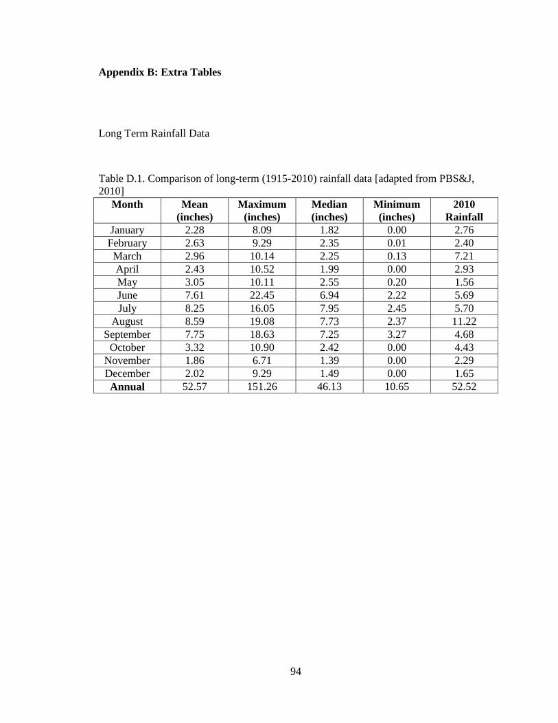
94
Appendix B: Extra Tables
Long Term Rainfall Data
Table D.1. Comparison of long-term (1915-2010) rainfall data [adapted from PBS&J,
2010]
Month Mean
(inches)
Maximum
(inches)
Median
(inches)
Minimum
(inches)
2010
Rainfall
January 2.28 8.09 1.82 0.00 2.76
February 2.63 9.29 2.35 0.01 2.40
March 2.96 10.14 2.25 0.13 7.21
April 2.43 10.52 1.99 0.00 2.93
May 3.05 10.11 2.55 0.20 1.56
June 7.61 22.45 6.94 2.22 5.69
July 8.25 16.05 7.95 2.45 5.70
August 8.59 19.08 7.73 2.37 11.22
September 7.75 18.63 7.25 3.27 4.68
October 3.32 10.90 2.42 0.00 4.43
November 1.86 6.71 1.39 0.00 2.29
December 2.02 9.29 1.49 0.00 1.65
Annual 52.57 151.26 46.13 10.65 52.52

95
Appendix C: SWMM-5 Input Parameters
Options
Flow units CFS
Infiltration Green
Ampt
Flow Routing Dynwave
Start date 6/3/1974
Start time 0:00:00
Report start date 6/3/1974
Report start time 0:00:00
End date 6/5/1974
End time 0:30:00
Sweep start 1-Jan
Sweep end 31-Dec
Dry days 10
Report step 0:30:00
Wet step 0:05:00
Dry step 1:00:00
Routing step yes
Allow ponding none
Inertial damping None
Variable step 0.75
Lengthening step 0
Min surface area 0 Norm flow
limited Both
Skip steady state none
Force main eq D-W
Link offsets Depth
Min-slope 0
Figure C.1. Options dialog box input parameters.
Evaporation
Type Parameter
Constant 0
Dry only No
Figure C.2. Evaporation input parameters.
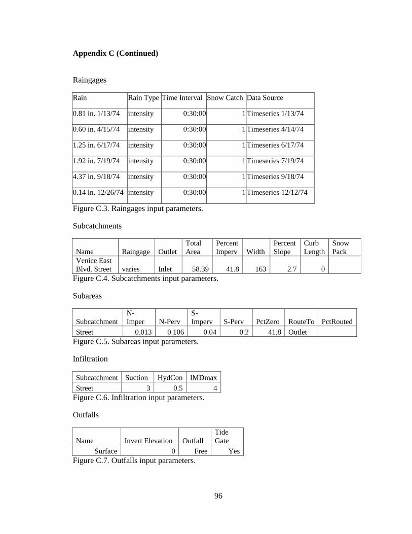
96
Appendix C (Continued)
Raingages
Rain Rain Type Time Interval Snow Catch Data Source
0.81 in. 1/13/74 intensity 0:30:00 1 Timeseries 1/13/74
0.60 in. 4/15/74 intensity 0:30:00 1 Timeseries 4/14/74
1.25 in. 6/17/74 intensity 0:30:00 1 Timeseries 6/17/74
1.92 in. 7/19/74 intensity 0:30:00 1 Timeseries 7/19/74
4.37 in. 9/18/74 intensity 0:30:00 1 Timeseries 9/18/74
0.14 in. 12/26/74 intensity 0:30:00 1 Timeseries 12/12/74
Figure C.3. Raingages input parameters.
Subcatchments
Name Raingage Outlet Total
Area Percent
Imperv Width Percent
Slope Curb
Length Snow
Pack Venice East
Blvd. Street varies Inlet 58.39 41.8 163 2.7 0
Figure C.4. Subcatchments input parameters.
Subareas
Subcatchment N-
Imper N-Perv S-
Imperv S-Perv PctZero RouteTo PctRouted
Street 0.013 0.106 0.04 0.2 41.8 Outlet
Figure C.5. Subareas input parameters.
Infiltration
Subcatchment Suction HydCon IMDmax
Street 3 0.5 4
Figure C.6. Infiltration input parameters.
Outfalls
Name Invert Elevation Outfall Tide
Gate
Surface 0 Free Yes
Figure C.7. Outfalls input parameters.
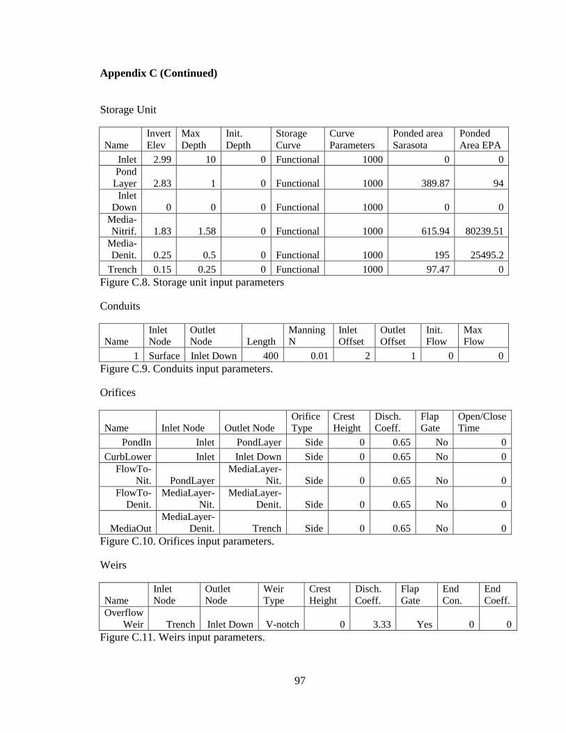
97
Appendix C (Continued)
Storage Unit
Name Invert
Elev Max
Depth Init.
Depth Storage
Curve Curve
Parameters Ponded area
Sarasota Ponded
Area EPA
Inlet 2.99 10 0 Functional 1000 0 0 Pond
Layer 2.83 1 0 Functional 1000 389.87 94 Inlet
Down 0 0 0 Functional 1000 0 0 Media-
Nitrif. 1.83 1.58 0 Functional 1000 615.94 80239.51 Media-
Denit. 0.25 0.5 0 Functional 1000 195 25495.2
Trench 0.15 0.25 0 Functional 1000 97.47 0
Figure C.8. Storage unit input parameters
Conduits
Name Inlet
Node Outlet
Node Length Manning
N Inlet
Offset Outlet
Offset Init.
Flow Max
Flow
1 Surface Inlet Down 400 0.01 2 1 0 0
Figure C.9. Conduits input parameters.
Orifices
Name Inlet Node Outlet Node Orifice
Type Crest
Height Disch.
Coeff. Flap
Gate Open/Close
Time
PondIn Inlet PondLayer Side 0 0.65 No 0
CurbLower Inlet Inlet Down Side 0 0.65 No 0 FlowTo-
Nit. PondLayer MediaLayer-
Nit. Side 0 0.65 No 0 FlowTo-
Denit. MediaLayer-
Nit. MediaLayer-
Denit. Side 0 0.65 No 0
MediaOut MediaLayer-
Denit. Trench Side 0 0.65 No 0
Figure C.10. Orifices input parameters.
Weirs
Name Inlet
Node Outlet
Node Weir
Type Crest
Height Disch.
Coeff. Flap
Gate End
Con. End
Coeff. Overflow
Weir Trench Inlet Down V-notch 0 3.33 Yes 0 0
Figure C.11. Weirs input parameters.

98
Appendix C (Continued)
XSections
Link Shape Geom1 Geom2 Geom3 Geom4 Barrels
1 Circular 1 0 0 0 1
PondIn Circular 2.83 0 0 0 0
CurbLower Circular 3.25 0 0 0 0
FlowTo-Nit. Circular 1.83 0 0 0 0 FlowTo-
Denit Circular 0.25 0 0 0 0
MediaOut Circular 0.15 0 0 0 0 Overflow
Weir Circular 1.5 1 0 0 0
Figure C.12. XSections input parameters.
Pollutants
Name Mass
units Rain
Conc. GW Conc. I&I
Conc. Snow
Only Co-
Pollutant DWF
Conc.
TKNi mg/L Input
value 0 0 0 * 0
NO3i mg/L Input
Value 0 0 0 TKNi 0
NO3 mg/L Input
Value 0 0 0 NO3i 0
Figure C.13. Pollutants input parameters.
Landuses
Name Cleaning Interval Fraction Avail. Last Cleaned Single Family
Residential 0 0 0
Figure C.14. Landuses input parameters.
Washoff
Land Use Pollutant Function Coeff. 1 Coeff. 2 Cleaning
Effic. BMP Effic. Single Family
Residential TKNi EMC 0.1 0 0 0 Single Family
Residential NO3i EMC 0 0 0 0 Single Family
Residential NO3 EMC 0 0 0 0
Figure C.15. Washoff input parameters.

99
Appendix C (Continued)
Treatment
Treatment Pollutant Function
MediaLayer-Nitrification TKNi C= (TKNi)*exp(-0.81*HRT)
MediaLayer-Denitrification NO3 C= (NO3i +R_TKNi)*exp(-2.5*HRT)
Figure C.16. Treatment input parameters.

100
Appendix D: SWMM-5 Water Quality Output Data
Quality Routing Results: analyses using the minimum concentrations
************************** TKNi NO3i NO3 Quality Routing Continuity lbs lbs lbs ************************** ---------- ---------- ---------- Dry Weather Inflow ....... 0.000 0.000 0.000 Wet Weather Inflow ....... 0.761 0.005 0.005 Groundwater Inflow ....... 0.000 0.000 0.000
RDII Inflow .............. 0.000 0.000 0.000
External Inflow .......... 0.000 0.000 0.000 Internal Flooding ........ 0.653 0.005 0.004 External Outflow ......... 0.000 0.000 0.000 Mass Reacted ............. 0.260 0.026 0.007 Initial Stored Mass ...... 0.000 0.000 0.000 Final Stored Mass ........ 0.000 0.000 0.000 Continuity Error (%) ..... -19.946 -519.045 -129.052
Figure D.1. Simulation using minimum concentration in Sarasota sized ABC model for
the 1/13/74 storm event.
************************** TKNi NO3i NO3 Quality Routing Continuity lbs lbs lbs ************************** ---------- ---------- ---------- Dry Weather Inflow ....... 0.000 0.000 0.000 Wet Weather Inflow ....... 0.762 0.005 0.005 Groundwater Inflow ....... 0.000 0.000 0.000 RDII Inflow .............. 0.000 0.000 0.000
External Inflow .......... 0.000 0.000 0.000 Internal Flooding ........ 0.648 0.005 0.004 External Outflow ......... 0.000 0.000 0.000
Mass Reacted ............. 0.966 0.110 0.006 Initial Stored Mass ...... 0.000 0.000 0.000 Final Stored Mass ........ 0.001 0.000 0.000 Continuity Error (%) ..... -111.918 -2189.876 -107.867
Figure D.2. Simulation using minimum concentration in EPA sized ABC model for the
1/13/74 storm event.

101
Appendix D (Continued)
************************** TKNi NO3i NO3 Quality Routing Continuity lbs lbs lbs ************************** ---------- ---------- ---------- Dry Weather Inflow ....... 0.000 0.000 0.000 Wet Weather Inflow ....... 0.551 0.004 0.004 Groundwater Inflow ....... 0.000 0.000 0.000 RDII Inflow .............. 0.000 0.000 0.000 External Inflow .......... 0.000 0.000 0.000 Internal Flooding ........ 0.460 0.004 0.003 External Outflow ......... 0.000 0.000 0.000
Mass Reacted ............. 0.241 0.023 0.006 Initial Stored Mass ...... 0.000 0.000 0.000
Final Stored Mass ........ 0.000 0.000 0.000 Continuity Error (%) ..... -27.268 -648.419 -155.467
Figure D.3. Simulation using minimum concentration in Sarasota sized ABC model for
the 4/15/74 storm event.
************************** TKNi NO3i NO3 Quality Routing Continuity lbs lbs lbs ************************** ---------- ---------- ---------- Dry Weather Inflow ....... 0.000 0.000 0.000
Wet Weather Inflow ....... 0.551 0.004 0.003 Groundwater Inflow ....... 0.000 0.000 0.000 RDII Inflow .............. 0.000 0.000 0.000 External Inflow .......... 0.000 0.000 0.000 Internal Flooding ........ 0.462 0.004 0.002 External Outflow ......... 0.000 0.000 0.000 Mass Reacted ............. 0.861 0.085 0.005 Initial Stored Mass ...... 0.000 0.000 0.000 Final Stored Mass ........ 0.000 0.000 0.000 Continuity Error (%) ..... -140.000 -2379.841 -122.735
Figure D.4. Simulation using minimum concentration in EPA sized ABC model for the
4/15/74 storm event.

102
Appendix D (Continued)
************************** TKNi NO3i NO3 Quality Routing Continuity lbs lbs lbs ************************** ---------- ---------- ---------- Dry Weather Inflow ....... 0.000 0.000 0.000 Wet Weather Inflow ....... 1.202 0.008 0.008 Groundwater Inflow ....... 0.000 0.000 0.000 RDII Inflow .............. 0.000 0.000 0.000 External Inflow .......... 0.000 0.000 0.000 Internal Flooding ........ 1.082 0.008 0.007 External Outflow ......... 0.000 0.000 0.000
Mass Reacted ............. 0.274 0.028 0.008 Initial Stored Mass ...... 0.000 0.000 0.000 Final Stored Mass ........ 0.000 0.000 0.000 Continuity Error (%) ..... -12.844 -348.307 -89.883
Figure D.5. Simulation using minimum concentration in Sarasota sized ABC model for
the 6/17/74 storm event.
************************** TKNi NO3i NO3 Quality Routing Continuity lbs lbs lbs ************************** ---------- ---------- ----------
Dry Weather Inflow ....... 0.000 0.000 0.000 Wet Weather Inflow ....... 1.203 0.008 0.007 Groundwater Inflow ....... 0.000 0.000 0.000 RDII Inflow .............. 0.000 0.000 0.000 External Inflow .......... 0.000 0.000 0.000 Internal Flooding ........ 0.983 0.008 0.006 External Outflow ......... 0.000 0.000 0.000 Mass Reacted ............. 0.972 0.133 0.010 Initial Stored Mass ...... 0.000 0.000 0.000 Final Stored Mass ........ 0.001 0.000 0.000 Continuity Error (%) ..... -62.574 -1644.763 -123.126
Figure D.6. Simulation using minimum concentration in EPA sized ABC model for the
6/17/74 storm event.

103
Appendix D (Continued)
************************** TKNi NO3i NO3 Quality Routing Continuity lbs lbs lbs ************************** ---------- ---------- ---------- Dry Weather Inflow ....... 0.000 0.000 0.000 Wet Weather Inflow ....... 1.873 0.013 0.013 Groundwater Inflow ....... 0.000 0.000 0.000 RDII Inflow .............. 0.000 0.000 0.000 External Inflow .......... 0.000 0.000 0.000 Internal Flooding ........ 1.741 0.013 0.012 External Outflow ......... 0.000 0.000 0.000
Mass Reacted ............. 0.309 0.032 0.010 Initial Stored Mass ...... 0.000 0.000 0.000 Final Stored Mass ........ 0.000 0.000 0.000 Continuity Error (%) ..... -9.480 -251.968 -68.246
Figure D.7. Simulation using minimum concentration in Sarasota sized ABC model for
the 7/19/74 storm event.
************************* TKNi NO3i NO3 Quality Routing Continuity lbs lbs lbs ************************** ---------- ---------- ----------
Dry Weather Inflow ....... 0.000 0.000 0.000 Wet Weather Inflow ....... 1.874 0.013 0.011 Groundwater Inflow ....... 0.000 0.000 0.000 RDII Inflow .............. 0.000 0.000 0.000 External Inflow .......... 0.000 0.000 0.000 Internal Flooding ........ 1.497 0.013 0.010 External Outflow ......... 0.000 0.000 0.000 Mass Reacted ............. 1.239 0.188 0.019 Initial Stored Mass ...... 0.000 0.000 0.000 Final Stored Mass ........ 0.001 0.000 0.000 Continuity Error (%) ..... -46.053 -1484.363 -159.169
Figure D.8. Simulation using minimum concentration in EPA sized ABC model for the
7/19/74 storm event.

104
Appendix D (Continued)
************************** TKNi NO3i NO3 Quality Routing Continuity lbs lbs lbs ************************** ---------- ---------- ---------- Dry Weather Inflow ....... 0.000 0.000 0.000 Wet Weather Inflow ....... 4.323 0.030 0.030 Groundwater Inflow ....... 0.000 0.000 0.000 RDII Inflow .............. 0.000 0.000 0.000 External Inflow .......... 0.000 0.000 0.000 Internal Flooding ........ 4.120 0.030 0.028 External Outflow ......... 0.000 0.000 0.000
Mass Reacted ............. 0.498 0.053 0.017 Initial Stored Mass ...... 0.000 0.000 0.000 Final Stored Mass ........ 0.001 0.000 0.000 Continuity Error (%) ..... -6.844 -179.537 -53.690
Figure D.9. Simulation using minimum concentration in Sarasota sized ABC model for
the 9/18/74 storm event.
************************** TKNi NO3i NO3 Quality Routing Continuity lbs lbs lbs ************************** ---------- ---------- ----------
Dry Weather Inflow ....... 0.000 0.000 0.000 Wet Weather Inflow ....... 4.324 0.030 0.027 Groundwater Inflow ....... 0.000 0.000 0.000 RDII Inflow .............. 0.000 0.000 0.000 External Inflow .......... 0.000 0.000 0.000 Internal Flooding ........ 3.487 0.029 0.025 External Outflow ......... 0.000 0.000 0.000 Mass Reacted ............. 2.315 0.461 0.067 Initial Stored Mass ...... 0.000 0.000 0.000 Final Stored Mass ........ 0.011 0.000 0.000 Continuity Error (%) ..... -34.409 -1556.887 -242.549
Figure D.10. Simulation using minimum concentration in EPA sized ABC model for the
9/18/74 storm event.

105
Appendix D (Continued)
************************** TKNi NO3i NO3 Quality Routing Continuity lbs lbs lbs ************************** ---------- ---------- ---------- Dry Weather Inflow ....... 0.000 0.000 0.000 Wet Weather Inflow ....... 0.090 0.000 0.000 Groundwater Inflow ....... 0.000 0.000 0.000 RDII Inflow .............. 0.000 0.000 0.000 External Inflow .......... 0.000 0.000 0.000 Internal Flooding ........ 0.067 0.000 0.000 External Outflow ......... 0.000 0.000 0.000
Mass Reacted ............. 0.111 0.006 0.001 Initial Stored Mass ...... 0.000 0.000 0.000 Final Stored Mass ........ 0.000 0.000 0.000 Continuity Error (%) ..... -98.686 -1473.505 -220.507
Figure D.11. Simulation using minimum concentration in Sarasota sized ABC model for
the 12/26/74 storm event.
************************** TKNi NO3i NO3 Quality Routing Continuity lbs lbs lbs ************************** ---------- ---------- ----------
Dry Weather Inflow ....... 0.000 0.000 0.000 Wet Weather Inflow ....... 0.091 0.000 0.000 Groundwater Inflow ....... 0.000 0.000 0.000 RDII Inflow .............. 0.000 0.000 0.000 External Inflow .......... 0.000 0.000 0.000 Internal Flooding ........ 0.068 0.000 0.000 External Outflow ......... 0.000 0.000 0.000 Mass Reacted ............. 0.114 0.006 0.001 Initial Stored Mass ...... 0.000 0.000 0.000 Final Stored Mass ........ 0.000 0.000 0.000 Continuity Error (%) ..... -100.975 -1496.250 -226.824
Figure D.12. Simulation using minimum concentration in EPA sized ABC model for the
12/26/74 storm event.

106
Appendix D (Continued)
Quality Routing Results: analyses using the median concentrations
************************** TKNi NO3i NO3 Quality Routing Continuity lbs lbs lbs ************************** ---------- ---------- ---------- Dry Weather Inflow ....... 0.000 0.000 0.000 Wet Weather Inflow ....... 11.740 0.887 0.005 Groundwater Inflow ....... 0.000 0.000 0.000 RDII Inflow .............. 0.000 0.000 0.000
External Inflow .......... 0.000 0.000 0.000 Internal Flooding ........ 10.070 0.884 0.004 External Outflow ......... 0.000 0.000 0.000 Mass Reacted ............. 4.008 5.282 0.007 Initial Stored Mass ...... 0.000 0.000 0.000 Final Stored Mass ........ 0.006 0.003 0.000 Continuity Error (%) ..... -19.964 -595.659 -132.470
Figure D.13. Simulation using median concentration in Sarasota sized ABC model for the
1/13/74 storm event.
************************** TKNi NO3i NO3
Quality Routing Continuity lbs lbs lbs ************************** ---------- ---------- ---------- Dry Weather Inflow ....... 0.000 0.000 0.000 Wet Weather Inflow ....... 11.754 0.888 0.005 Groundwater Inflow ....... 0.000 0.000 0.000 RDII Inflow .............. 0.000 0.000 0.000 External Inflow .......... 0.000 0.000 0.000 Internal Flooding ........ 9.996 0.886 0.004 External Outflow ......... 0.000 0.000 0.000 Mass Reacted ............. 14.906 19.887 0.006 Initial Stored Mass ...... 0.000 0.000 0.000
Final Stored Mass ........ 0.009 0.003 0.000 Continuity Error (%) ..... -111.934 -2240.175 -110.546
Figure D.14. Simulation using median concentration in EPA sized ABC model for the
1/13/74 storm event.

107
Appendix D (Continued)
************************** TKNi NO3i NO3 Quality Routing Continuity lbs lbs lbs ************************** ---------- ---------- ---------- Dry Weather Inflow ....... 0.000 0.000 0.000 Wet Weather Inflow ....... 8.497 0.642 0.004 Groundwater Inflow ....... 0.000 0.000 0.000 RDII Inflow .............. 0.000 0.000 0.000 External Inflow .......... 0.000 0.000 0.000 Internal Flooding ........ 7.094 0.639 0.003 External Outflow ......... 0.000 0.000 0.000
Mass Reacted ............. 3.716 4.807 0.006 Initial Stored Mass ...... 0.000 0.000 0.000 Final Stored Mass ........ 0.006 0.003 0.000 Continuity Error (%) ..... -27.290 -749.015 -160.867
Figure D.15. Simulation using median concentration in Sarasota sized ABC model for the
4/15/74 storm event.
************************** TKNi NO3i NO3 Quality Routing Continuity lbs lbs lbs ************************** ---------- ---------- ---------- Dry Weather Inflow ....... 0.000 0.000 0.000
Wet Weather Inflow ....... 8.511 0.643 0.003 Groundwater Inflow ....... 0.000 0.000 0.000 RDII Inflow .............. 0.000 0.000 0.000 External Inflow .......... 0.000 0.000 0.000 Internal Flooding ........ 7.135 0.641 0.002 External Outflow ......... 0.000 0.000 0.000 Mass Reacted ............. 13.283 15.578 0.005 Initial Stored Mass ...... 0.000 0.000 0.000 Final Stored Mass ........ 0.008 0.002 0.000 Continuity Error (%) ..... -140.005 -2423.720 -126.535
Figure D.16. Simulation using median concentration in EPA sized ABC model for the
4/15/74 storm event.

108
Appendix D (Continued)
************************** TKNi NO3i NO3 Quality Routing Continuity lbs lbs lbs ************************** ---------- ---------- ---------- Dry Weather Inflow ....... 0.000 0.000 0.000 Wet Weather Inflow ....... 18.545 1.401 0.008 Groundwater Inflow ....... 0.000 0.000 0.000 RDII Inflow .............. 0.000 0.000 0.000 External Inflow .......... 0.000 0.000 0.000 Internal Flooding ........ 16.637 1.398 0.008 External Outflow ......... 0.000 0.000 0.000
Mass Reacted ............. 4.496 2.704 0.009 Initial Stored Mass ...... 0.000 0.000 0.000 Final Stored Mass ........ 0.005 0.003 0.000 Continuity Error (%) ..... -13.983 -193.053 -105.494
Figure D.17. Simulation using median concentration in Sarasota sized ABC model for the
6/17/74 storm event.
************************** TKNi NO3i NO3 Quality Routing Continuity lbs lbs lbs ************************** ---------- ---------- ----------
Dry Weather Inflow ....... 0.000 0.000 0.000 Wet Weather Inflow ....... 18.559 1.402 0.007 Groundwater Inflow ....... 0.000 0.000 0.000 RDII Inflow .............. 0.000 0.000 0.000 External Inflow .......... 0.000 0.000 0.000 Internal Flooding ........ 15.163 1.405 0.006 External Outflow ......... 0.000 0.000 0.000 Mass Reacted ............. 15.005 23.760 0.010 Initial Stored Mass ...... 0.000 0.000 0.000 Final Stored Mass ........ 0.008 0.003 0.000 Continuity Error (%) ..... -62.594 -1695.243 -124.702
Figure D.18. Simulation using median concentration in EPA sized ABC model for the
6/17/74 storm event.

109
Appendix D (Continued)
************************** TKNi NO3i NO3 Quality Routing Continuity lbs lbs lbs ************************** ---------- ---------- ---------- Dry Weather Inflow ....... 0.000 0.000 0.000 Wet Weather Inflow ....... 28.899 2.183 0.013 Groundwater Inflow ....... 0.000 0.000 0.000 RDII Inflow .............. 0.000 0.000 0.000 External Inflow .......... 0.000 0.000 0.000 Internal Flooding ........ 26.867 2.181 0.012 External Outflow ......... 0.000 0.000 0.000
Mass Reacted ............. 4.768 6.264 0.010 Initial Stored Mass ...... 0.000 0.000 0.000 Final Stored Mass ........ 0.007 0.003 0.000 Continuity Error (%) ..... -9.488 -286.993 -69.424
Figure D.19. Simulation using median concentration in Sarasota sized ABC model for the
7/19/74 storm event.
************************** TKNi NO3i NO3 Quality Routing Continuity lbs lbs lbs ************************** ---------- ---------- ----------
Dry Weather Inflow ....... 0.000 0.000 0.000 Wet Weather Inflow ....... 28.914 2.184 0.011 Groundwater Inflow ....... 0.000 0.000 0.000 RDII Inflow .............. 0.000 0.000 0.000 External Inflow .......... 0.000 0.000 0.000 Internal Flooding ........ 23.103 2.183 0.010 External Outflow ......... 0.000 0.000 0.000 Mass Reacted ............. 19.120 33.337 0.020 Initial Stored Mass ...... 0.000 0.000 0.000 Final Stored Mass ........ 0.011 0.004 0.000 Continuity Error (%) ..... -46.070 -1526.405 -160.199
Figure D.20. Simulation using median concentration in EPA sized ABC model for the
7/19/74 storm event.

110
Appendix D (Continued)
************************** TKNi NO3i NO3 Quality Routing Continuity lbs lbs lbs ************************** ---------- ---------- ---------- Dry Weather Inflow ....... 0.000 0.000 0.000 Wet Weather Inflow ....... 66.694 5.038 0.030 Groundwater Inflow ....... 0.000 0.000 0.000 RDII Inflow .............. 0.000 0.000 0.000 External Inflow .......... 0.000 0.000 0.000 Internal Flooding ........ 63.571 5.038 0.028 External Outflow ......... 0.000 0.000 0.000
Mass Reacted ............. 7.682 9.745 0.017 Initial Stored Mass ...... 0.000 0.000 0.000 Final Stored Mass ........ 0.009 0.003 0.000 Continuity Error (%) ..... -6.848 -193.459 -54.250
Figure D.21. Simulation using median concentration in Sarasota sized ABC model for the
9/18/74 storm event.
************************** TKNi NO3i NO3 Quality Routing Continuity lbs lbs lbs ************************** ---------- ---------- ----------
Dry Weather Inflow ....... 0.000 0.000 0.000 Wet Weather Inflow ....... 66.714 5.040 0.027 Groundwater Inflow ....... 0.000 0.000 0.000 RDII Inflow .............. 0.000 0.000 0.000 External Inflow .......... 0.000 0.000 0.000 Internal Flooding ........ 53.794 4.973 0.025 External Outflow ......... 0.000 0.000 0.000 Mass Reacted ............. 35.719 79.793 0.067 Initial Stored Mass ...... 0.000 0.000 0.000 Final Stored Mass ........ 0.163 0.068 0.000 Continuity Error (%) ..... -34.419 -1583.250 -243.032
Figure D.22. Simulation using median concentration in EPA sized ABC model for the
9/18/74 storm event.

111
Appendix D (Continued)
************************** TKNi NO3i NO3 Quality Routing Continuity lbs lbs lbs ************************** ---------- ---------- ---------- Dry Weather Inflow ....... 0.000 0.000 0.000 Wet Weather Inflow ....... 1.392 0.105 0.000 Groundwater Inflow ....... 0.000 0.000 0.000 RDII Inflow .............. 0.000 0.000 0.000 External Inflow .......... 0.000 0.000 0.000 Internal Flooding ........ 1.042 0.102 0.000 External Outflow ......... 0.000 0.000 0.000
Mass Reacted ............. 1.718 1.955 0.001 Initial Stored Mass ...... 0.000 0.000 0.000 Final Stored Mass ........ 0.005 0.002 0.000 Continuity Error (%) ..... -98.701 -1863.335 -256.266
Figure D.23. Simulation using median concentration in Sarasota sized ABC model for the
12/26/74 storm event.
************************** TKNi NO3i NO3 Quality Routing Continuity lbs lbs lbs ************************** ---------- ---------- ----------
Dry Weather Inflow ....... 0.000 0.000 0.000 Wet Weather Inflow ....... 1.403 0.106 0.000 Groundwater Inflow ....... 0.000 0.000 0.000 RDII Inflow .............. 0.000 0.000 0.000 External Inflow .......... 0.000 0.000 0.000 Internal Flooding ........ 1.050 0.104 0.000 External Outflow ......... 0.000 0.000 0.000 Mass Reacted ............. 1.766 2.073 0.001 Initial Stored Mass ...... 0.000 0.000 0.000 Final Stored Mass ........ 0.004 0.002 0.000 Continuity Error (%) ..... -100.992 -1960.508 -267.090
Figure D.24. Simulation using median concentration in EPA sized ABC model for the
12/26/74 storm event.

112
Appendix D (Continued)
Quality Routing Results: analyses using the maximum concentrations
************************** TKNi NO3i NO3 Quality Routing Continuity lbs lbs lbs ************************** ---------- ---------- ---------- Dry Weather Inflow ....... 0.000 0.000 0.000 Wet Weather Inflow ....... 35.945 3.784 0.005 Groundwater Inflow ....... 0.000 0.000 0.000 RDII Inflow .............. 0.000 0.000 0.000
External Inflow .......... 0.000 0.000 0.000 Internal Flooding ........ 30.831 3.772 0.004 External Outflow ......... 0.000 0.000 0.000 Mass Reacted ............. 12.270 22.551 0.007 Initial Stored Mass ...... 0.000 0.000 0.000 Final Stored Mass ........ 0.019 0.012 0.000 Continuity Error (%) ..... -19.965 -595.994 -135.622
Figure D.25. Simulation using maximum concentration in Sarasota sized ABC model for
the 1/13/74 storm event.
************************** TKNi NO3i NO3
Quality Routing Continuity lbs lbs lbs ************************** ---------- ---------- ---------- Dry Weather Inflow ....... 0.000 0.000 0.000 Wet Weather Inflow ....... 35.988 3.788 0.005 Groundwater Inflow ....... 0.000 0.000 0.000 RDII Inflow .............. 0.000 0.000 0.000 External Inflow .......... 0.000 0.000 0.000 Internal Flooding ........ 30.604 3.782 0.004 External Outflow ......... 0.000 0.000 0.000 Mass Reacted ............. 45.640 84.868 0.006 Initial Stored Mass ...... 0.000 0.000 0.000
Final Stored Mass ........ 0.027 0.011 0.000 Continuity Error (%) ..... -111.934 -2240.395 -111.680
Figure D.26. Simulation using maximum concentration in EPA sized ABC model for the
1/13/74 storm event.

113
Appendix D (Continued)
************************** TKNi NO3i NO3 Quality Routing Continuity lbs lbs lbs ************************** ---------- ---------- ---------- Dry Weather Inflow ....... 0.000 0.000 0.000 Wet Weather Inflow ....... 26.017 2.739 0.004 Groundwater Inflow ....... 0.000 0.000 0.000 RDII Inflow .............. 0.000 0.000 0.000 External Inflow .......... 0.000 0.000 0.000 Internal Flooding ........ 21.720 2.727 0.003 External Outflow ......... 0.000 0.000 0.000
Mass Reacted ............. 11.378 20.524 0.006 Initial Stored Mass ...... 0.000 0.000 0.000 Final Stored Mass ........ 0.019 0.012 0.000 Continuity Error (%) ..... -27.291 -749.446 -165.146
Figure D.27. Simulation using maximum concentration in Sarasota sized ABC model for
the 4/15/74 storm event.
************************* TKNi NO3i NO3 Quality Routing Continuity lbs lbs lbs ************************** ---------- ---------- ---------- Dry Weather Inflow ....... 0.000 0.000 0.000
Wet Weather Inflow ....... 26.058 2.743 0.003 Groundwater Inflow ....... 0.000 0.000 0.000 RDII Inflow .............. 0.000 0.000 0.000 External Inflow .......... 0.000 0.000 0.000 Internal Flooding ........ 21.846 2.736 0.002 External Outflow ......... 0.000 0.000 0.000 Mass Reacted ............. 40.670 66.483 0.005 Initial Stored Mass ...... 0.000 0.000 0.000 Final Stored Mass ........ 0.023 0.010 0.000 Continuity Error (%) ..... -140.005 -2423.908 -128.069
Figure D.28. Simulation using maximum concentration in EPA sized ABC model for the
4/15/74 storm event.

114
Appendix D (Continued)
************************** TKNi NO3i NO3 Quality Routing Continuity lbs lbs lbs ************************** ---------- ---------- ---------- Dry Weather Inflow ....... 0.000 0.000 0.000 Wet Weather Inflow ....... 56.779 5.977 0.008 Groundwater Inflow ....... 0.000 0.000 0.000 RDII Inflow .............. 0.000 0.000 0.000 External Inflow .......... 0.000 0.000 0.000 Internal Flooding ........ 51.128 5.965 0.007 External Outflow ......... 0.000 0.000 0.000
Mass Reacted ............. 12.932 23.994 0.008 Initial Stored Mass ...... 0.000 0.000 0.000 Final Stored Mass ........ 0.019 0.012 0.000 Continuity Error (%) ..... -12.857 -401.448 -93.732
Figure D.29. Simulation using maximum concentration in Sarasota sized ABC model for
the 6/17/74 storm event.
************************** TKNi NO3i NO3 Quality Routing Continuity lbs lbs lbs ************************** ---------- ---------- ----------
Dry Weather Inflow ....... 0.000 0.000 0.000 Wet Weather Inflow ....... 56.822 5.982 0.007 Groundwater Inflow ....... 0.000 0.000 0.000 RDII Inflow .............. 0.000 0.000 0.000 External Inflow .......... 0.000 0.000 0.000 Internal Flooding ........ 46.425 5.993 0.006 External Outflow ......... 0.000 0.000 0.000 Mass Reacted ............. 45.941 101.391 0.010 Initial Stored Mass ...... 0.000 0.000 0.000 Final Stored Mass ........ 0.025 0.012 0.000 Continuity Error (%) ..... -62.595 -1695.467 -125.356
Figure D.30. Simulation using maximum concentration in EPA sized ABC model for the
6/17/74 storm event.

115
Appendix D (Continued)
************************** TKNi NO3i NO3 Quality Routing Continuity lbs lbs lbs ************************** ---------- ---------- ---------- Dry Weather Inflow ....... 0.000 0.000 0.000 Wet Weather Inflow ....... 88.479 9.314 0.013 Groundwater Inflow ....... 0.000 0.000 0.000 RDII Inflow .............. 0.000 0.000 0.000 External Inflow .......... 0.000 0.000 0.000 Internal Flooding ........ 82.257 9.307 0.012 External Outflow ......... 0.000 0.000 0.000
Mass Reacted ............. 14.597 26.740 0.010 Initial Stored Mass ...... 0.000 0.000 0.000 Final Stored Mass ........ 0.020 0.012 0.000 Continuity Error (%) ..... -9.489 -287.150 -70.488
Figure D.31. Simulation using maximum concentration in Sarasota sized ABC model for
the 7/19/74 storm event.
************************** TKNi NO3i NO3 Quality Routing Continuity lbs lbs lbs ************************** ---------- ---------- ----------
Dry Weather Inflow ....... 0.000 0.000 0.000 Wet Weather Inflow ....... 88.525 9.319 0.011 Groundwater Inflow ....... 0.000 0.000 0.000 RDII Inflow .............. 0.000 0.000 0.000 External Inflow .......... 0.000 0.000 0.000 Internal Flooding ........ 70.736 9.313 0.010 External Outflow ......... 0.000 0.000 0.000 Mass Reacted ............. 58.541 142.251 0.020 Initial Stored Mass ...... 0.000 0.000 0.000 Final Stored Mass ........ 0.032 0.016 0.000 Continuity Error (%) ..... -46.071 -1526.593 -160.628
Figure D.32. Simulation using maximum concentration in EPA sized ABC model for the
7/19/74 storm event.
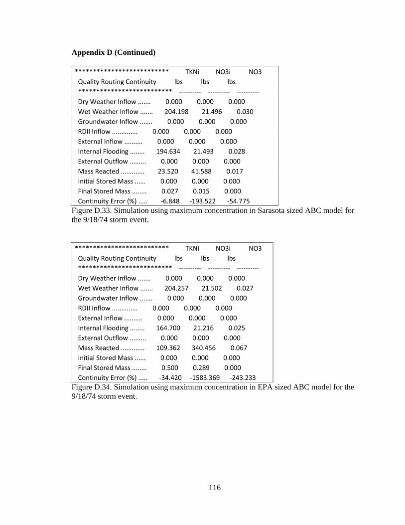
116
Appendix D (Continued)
************************** TKNi NO3i NO3 Quality Routing Continuity lbs lbs lbs ************************** ---------- ---------- ---------- Dry Weather Inflow ....... 0.000 0.000 0.000 Wet Weather Inflow ....... 204.198 21.496 0.030 Groundwater Inflow ....... 0.000 0.000 0.000 RDII Inflow .............. 0.000 0.000 0.000 External Inflow .......... 0.000 0.000 0.000 Internal Flooding ........ 194.634 21.493 0.028 External Outflow ......... 0.000 0.000 0.000
Mass Reacted ............. 23.520 41.588 0.017 Initial Stored Mass ...... 0.000 0.000 0.000 Final Stored Mass ........ 0.027 0.015 0.000 Continuity Error (%) ..... -6.848 -193.522 -54.775
Figure D.33. Simulation using maximum concentration in Sarasota sized ABC model for
the 9/18/74 storm event.
************************** TKNi NO3i NO3 Quality Routing Continuity lbs lbs lbs ************************** ---------- ---------- ----------
Dry Weather Inflow ....... 0.000 0.000 0.000 Wet Weather Inflow ....... 204.257 21.502 0.027 Groundwater Inflow ....... 0.000 0.000 0.000 RDII Inflow .............. 0.000 0.000 0.000 External Inflow .......... 0.000 0.000 0.000 Internal Flooding ........ 164.700 21.216 0.025 External Outflow ......... 0.000 0.000 0.000 Mass Reacted ............. 109.362 340.456 0.067 Initial Stored Mass ...... 0.000 0.000 0.000 Final Stored Mass ........ 0.500 0.289 0.000 Continuity Error (%) ..... -34.420 -1583.369 -243.233
Figure D.34. Simulation using maximum concentration in EPA sized ABC model for the
9/18/74 storm event.

117
Appendix D (Continued)
************************** TKNi NO3i NO3 Quality Routing Continuity lbs lbs lbs ************************** ---------- ---------- ---------- Dry Weather Inflow ....... 0.000 0.000 0.000 Wet Weather Inflow ....... 4.261 0.448 0.000 Groundwater Inflow ....... 0.000 0.000 0.000 RDII Inflow .............. 0.000 0.000 0.000 External Inflow .......... 0.000 0.000 0.000 Internal Flooding ........ 3.192 0.438 0.000 External Outflow ......... 0.000 0.000 0.000
Mass Reacted ............. 5.259 8.360 0.001 Initial Stored Mass ...... 0.000 0.000 0.000 Final Stored Mass ........ 0.016 0.011 0.000 Continuity Error (%) ..... -98.702 -1864.467 -271.730
Figure D.35. Simulation using maximum concentration in Sarasota sized ABC model for
the 12/26/74 storm event.
************************** TKNi NO3i NO3 Quality Routing Continuity lbs lbs lbs ************************** ---------- ---------- ----------
Dry Weather Inflow ....... 0.000 0.000 0.000 Wet Weather Inflow ....... 4.295 0.452 0.000 Groundwater Inflow ....... 0.000 0.000 0.000 RDII Inflow .............. 0.000 0.000 0.000 External Inflow .......... 0.000 0.000 0.000 Internal Flooding ........ 3.214 0.443 0.000 External Outflow ......... 0.000 0.000 0.000 Mass Reacted ............. 5.407 8.866 0.001 Initial Stored Mass ...... 0.000 0.000 0.000 Final Stored Mass ........ 0.012 0.009 0.000 Continuity Error (%) ..... -100.992 -1961.845 -283.809
Figure D.36. Simulation using maximum concentration in EPA sized ABC model for the
12/26/74 storm event.

118
Appendix D (Continued)
Quality Routing Results: analyses using the analyzed concentrations
************************** TKNi NO3i NO3 Quality Routing Continuity lbs lbs lbs ************************** ---------- ---------- ------- Dry Weather Inflow ....... 0.000 0.000 0.000 Wet Weather Inflow ....... 6.156 3.112 0.005 Groundwater Inflow ....... 0.000 0.000 0.000 RDII Inflow .............. 0.000 0.000 0.000
External Inflow .......... 0.000 0.000 0.000 Internal Flooding ........ 5.244 3.102 0.005 External Outflow ......... 0.000 0.000 0.000 Mass Reacted ............. 2.231 8.924 0.008 Initial Stored Mass ...... 0.000 0.000 0.000 Final Stored Mass ........ 0.003 0.010 0.000 Continuity Error (%) ..... -21.477 -286.766 -154.558
Figure D.37. Simulation using analyzed concentration in Sarasota sized ABC model for
the 1/13/74 storm event.
************************** TKNi NO3i NO3 Quality Routing Continuity lbs lbs lbs ************************** ---------- ---------- ---------- Dry Weather Inflow ....... 0.000 0.000 0.000 Wet Weather Inflow ....... 6.163 3.116 0.005 Groundwater Inflow ....... 0.000 0.000 0.000
RDII Inflow .............. 0.000 0.000 0.000 External Inflow .......... 0.000 0.000 0.000 Internal Flooding ........ 5.241 3.111 0.004 External Outflow ......... 0.000 0.000 0.000 Mass Reacted ............. 7.816 69.800 0.006
Initial Stored Mass ...... 0.000 0.000 0.000 Final Stored Mass ........ 0.005 0.009 0.000 Continuity Error (%) ..... -111.933 -2240.380 -110.533
Figure D.38. Simulation using analyzed concentration in EPA sized ABC model for the
1/13/74 storm event.

119
Appendix D (Continued)
************************** TKNi NO3i NO3 Quality Routing Continuity lbs lbs lbs ************************** ---------- ---------- ---------- Dry Weather Inflow ....... 0.000 0.000 0.000 Wet Weather Inflow ....... 4.456 2.252 0.004 Groundwater Inflow ....... 0.000 0.000 0.000 RDII Inflow .............. 0.000 0.000 0.000 External Inflow .......... 0.000 0.000 0.000 Internal Flooding ........ 3.720 2.243 0.003 External Outflow ......... 0.000 0.000 0.000
Mass Reacted ............. 1.948 16.880 0.006 Initial Stored Mass ...... 0.000 0.000 0.000 Final Stored Mass ........ 0.003 0.010 0.000 Continuity Error (%) ..... -27.289 -749.418 -161.013
Figure D.39. Simulation using analyzed concentration in Sarasota sized ABC model for
the 4/15/74 storm event.
************************** TKNi NO3i NO3 Quality Routing Continuity lbs lbs lbs ************************** ---------- ---------- ---------- Dry Weather Inflow ....... 0.000 0.000 0.000
Wet Weather Inflow ....... 4.463 2.256 0.003 Groundwater Inflow ....... 0.000 0.000 0.000 RDII Inflow .............. 0.000 0.000 0.000 External Inflow .......... 0.000 0.000 0.000 Internal Flooding ........ 3.678 2.250 0.002 External Outflow ......... 0.000 0.000 0.000 Mass Reacted ............. 7.270 26.310 0.005 Initial Stored Mass ...... 0.000 0.000 0.000 Final Stored Mass ........ 0.003 0.008 0.000 Continuity Error (%) ..... -145.413 -1166.363 -136.526
Figure D.40. Simulation using analyzed concentration in EPA sized ABC model for the
4/15/74 storm event.

120
Appendix D (Continued)
************************** TKNi NO3i NO3 Quality Routing Continuity lbs lbs lbs ************************** ---------- ---------- ---------- Dry Weather Inflow ....... 0.000 0.000 0.000 Wet Weather Inflow ....... 9.724 4.916 0.008 Groundwater Inflow ....... 0.000 0.000 0.000 RDII Inflow .............. 0.000 0.000 0.000 External Inflow .......... 0.000 0.000 0.000 Internal Flooding ........ 8.756 4.906 0.007 External Outflow ......... 0.000 0.000 0.000
Mass Reacted ............. 2.215 19.734 0.008 Initial Stored Mass ...... 0.000 0.000 0.000 Final Stored Mass ........ 0.003 0.010 0.000 Continuity Error (%) ..... -12.855 -401.433 -92.287
Figure D.41. Simulation using analyzed concentration in Sarasota sized ABC model for
the 6/17/74 storm event.
************************** TKNi NO3i NO3 Quality Routing Continuity lbs lbs lbs ************************** ---------- ---------- ---------- Dry Weather Inflow ....... 0.000 0.000 0.000
Wet Weather Inflow ....... 9.732 4.920 0.007 Groundwater Inflow ....... 0.000 0.000 0.000 RDII Inflow .............. 0.000 0.000 0.000 External Inflow .......... 0.000 0.000 0.000 Internal Flooding ........ 7.951 4.929 0.006 External Outflow ......... 0.000 0.000 0.000 Mass Reacted ............. 7.868 83.390 0.010 Initial Stored Mass ...... 0.000 0.000 0.000 Final Stored Mass ........ 0.004 0.010 0.000 Continuity Error (%) ..... -62.593 -1695.452 -124.738
Figure D.42. Simulation using analyzed concentration in EPA sized ABC model for the
6/17/74 storm event.

121
Appendix D (Continued)
************************** TKNi NO3i NO3 Quality Routing Continuity lbs lbs lbs ************************** ---------- ---------- ---------- Dry Weather Inflow ....... 0.000 0.000 0.000 Wet Weather Inflow ....... 15.153 7.661 0.013 Groundwater Inflow ....... 0.000 0.000 0.000 RDII Inflow .............. 0.000 0.000 0.000 External Inflow .......... 0.000 0.000 0.000 Internal Flooding ........ 14.088 7.655 0.012 External Outflow ......... 0.000 0.000 0.000
Mass Reacted ............. 2.500 21.992 0.010 Initial Stored Mass ...... 0.000 0.000 0.000 Final Stored Mass ........ 0.003 0.010 0.000 Continuity Error (%) ..... -9.488 -287.139 -69.718
Figure D.43. Simulation using analyzed concentration in Sarasota sized ABC model for
the 7/19/74 storm event.
************************** TKNi NO3i NO3 Quality Routing Continuity lbs lbs lbs ************************** ---------- ---------- ---------- Dry Weather Inflow ....... 0.000 0.000 0.000
Wet Weather Inflow ....... 15.161 7.664 0.011 Groundwater Inflow ....... 0.000 0.000 0.000 RDII Inflow .............. 0.000 0.000 0.000 External Inflow .......... 0.000 0.000 0.000 Internal Flooding ........ 12.114 7.660 0.010 External Outflow ......... 0.000 0.000 0.000 Mass Reacted ............. 10.026 116.996 0.020 Initial Stored Mass ...... 0.000 0.000 0.000 Final Stored Mass ........ 0.006 0.013 0.000 Continuity Error (%) ..... -46.069 -1526.581 -160.183
Figure D.44. Simulation using analyzed concentration in EPA sized ABC model for the
7/19/74 storm event.

122
Appendix D (Continued)
************************** TKNi NO3i NO3 Quality Routing Continuity lbs lbs lbs ************************** ---------- ---------- ---------- Dry Weather Inflow ....... 0.000 0.000 0.000 Wet Weather Inflow ....... 34.972 17.680 0.030 Groundwater Inflow ....... 0.000 0.000 0.000 RDII Inflow .............. 0.000 0.000 0.000 External Inflow .......... 0.000 0.000 0.000 Internal Flooding ........ 33.334 17.677 0.028 External Outflow ......... 0.000 0.000 0.000
Mass Reacted ............. 4.028 34.204 0.017 Initial Stored Mass ...... 0.000 0.000 0.000 Final Stored Mass ........ 0.005 0.012 0.000 Continuity Error (%) ..... -6.847 -193.517 -54.441
Figure D.45. Simulation using analyzed concentration in Sarasota sized ABC model for
the 9/18/74 storm event.
************************** TKNi NO3i NO3 Quality Routing Continuity lbs lbs lbs ************************** ---------- ---------- ---------- Dry Weather Inflow ....... 0.000 0.000 0.000
Wet Weather Inflow ....... 34.982 17.685 0.027 Groundwater Inflow ....... 0.000 0.000 0.000 RDII Inflow .............. 0.000 0.000 0.000 External Inflow .......... 0.000 0.000 0.000 Internal Flooding ........ 28.207 17.449 0.025 External Outflow ......... 0.000 0.000 0.000 Mass Reacted ............. 18.729 280.012 0.067 Initial Stored Mass ...... 0.000 0.000 0.000 Final Stored Mass ........ 0.086 0.237 0.000 Continuity Error (%) ..... -34.419 -1583.361 -243.008
Figure D.46. Simulation using analyzed concentration in EPA sized ABC model for the
9/18/74 storm event.

123
Appendix D (Continued)
************************** TKNi NO3i NO3 Quality Routing Continuity lbs lbs lbs ************************** ---------- ---------- ---------- Dry Weather Inflow ....... 0.000 0.000 0.000 Wet Weather Inflow ....... 0.730 0.369 0.000 Groundwater Inflow ....... 0.000 0.000 0.000 RDII Inflow .............. 0.000 0.000 0.000 External Inflow .......... 0.000 0.000 0.000 Internal Flooding ........ 0.546 0.360 0.000 External Outflow ......... 0.000 0.000 0.000
Mass Reacted ............. 0.901 6.875 0.001 Initial Stored Mass ...... 0.000 0.000 0.000 Final Stored Mass ........ 0.003 0.009 0.000 Continuity Error (%) ..... -98.700 -1864.393 -254.510
Figure D.47. Simulation using analyzed concentration in Sarasota sized ABC model for
the 12/26/74 storm event.
************************** TKNi NO3i NO3 Quality Routing Continuity lbs lbs lbs ************************** ---------- ---------- ---------- Dry Weather Inflow ....... 0.000 0.000 0.000
Wet Weather Inflow ....... 0.735 0.372 0.000 Groundwater Inflow ....... 0.000 0.000 0.000 RDII Inflow .............. 0.000 0.000 0.000 External Inflow .......... 0.000 0.000 0.000 Internal Flooding ........ 0.550 0.364 0.000 External Outflow ......... 0.000 0.000 0.000 Mass Reacted ............. 0.926 7.291 0.001 Initial Stored Mass ...... 0.000 0.000 0.000 Final Stored Mass ........ 0.002 0.007 0.000 Continuity Error (%) ..... -100.991 -1961.757 -265.172
Figure D.48. Simulation using analyzed concentration in EPA sized ABC model for the
12/26/74 storm event.

About the Author
Michelle Masi was born in Florida and earned her Bachelor of Science in
Environmental Science from the University of South Florida. Academically, Michelle has
gained an interdisciplinary skill set by taking courses in public health, water resources,
environmental sciences, statistics and experimental design. Her research experience
includes the development of a stochastic, age-based population model to assess Florida
manatee population dynamics at the Florida Fish & Wildlife Research Institute. She has
worked as a Environmental Engineer for the Florida Department of Environmental
Protection, reviewing engineer drawings and applications for the development and repair
of municipal water and wastewater systems. Michelle was recently awarded an S_STEM
scholarship for academically talented graduate students from the College Engineering‟s
Department of Civil and Environmental Engineering.